Best Practices for Preparing Environmental Data Sets to Share and Archive1

Les A. Hook, Suresh K. Santhana Vannan, Tammy W. Beaty, Robert B. Cook, and Bruce E. Wilson September 2010

Oak Ridge National Laboratory Distributed Active Archive Center, Oak Ridge, Tennessee, U.S.A.

Environmental Sciences Division, Oak Ridge National Laboratory2

[ Go to Best Practices - Section 2 ]

1 Introduction

At the request of field researchers, investigators, GIS and image specialists, and data managers, we prepared the following data management practices that data collectors and providers should follow to improve the usability of their data sets. This guidance is provided for those who perform environmental measurements, compile data from various sources, prepare GIS coverages, and compile remote sensing images for environmental applications, although many of the practices may be useful for other data collection and archiving activities.

We assembled what we feel are the most important practices that researchers could implement to make their data sets ready to share with other researchers. These practices could be performed at any time during the preparation of the data set, but we suggest that researchers plan for them before measurements are taken and implement them during measurements. The order of the practices is not necessarily sequential, as a researcher could provide draft data set metadata before any measurements are taken based on their planning. We introduce topics in the sections that follow and if additional resources are available, they are included in an Appendix.

1.1 Scope

The life cycle for collection or generation of environmental data can be configured and represented in various graphical ways. All approaches have steps for research design and data management planning, the collection or generation of data and its processing and analysis, the preparation of data for sharing and dissemination, and the archiving of the data with metadata and documentation. The feedback and use of existing archived data at any and all steps along the data flow closes the loop.

1 or Preparing Ecological and Ground-Based Data Sets to Share and Archive," C

PBoA

2

cA

Previously entitled "Best Practices f

ook, et al., 2001. Web version was previously updated in 2007.

lease cite this document as: Hook, Les A., Suresh K. Santhana Vannan, Tammy W. Beaty, Robert B. Cook, and ruce E. Wilson. 2010. Best Practices for Preparing Environmental Data Sets to Share and Archive. Available nline (http://daac.ornl.gov/PI/BestPractices-2010.pdf) from Oak Ridge National Laboratory Distributed Active rchive Center, Oak Ridge, Tennessee, U.S.A. doi:10.3334/ORNLDAAC/BestPractices-2010

Oak Ridge National Laboratory is operated by UT-Battelle, LLC, for the U.S. Department of Energy under ontract DE-AC05-00OR22725. This work was sponsored by the U.S. National Aeronautics and Space dministration, Earth Science Data and Information Systems Project.

1

This work is licensed under a Creative Commons Attribution 3.0 Unported License.

This best practices guide does not attempt to cover the complete data life cycle (DDI, 2010; MIT Libraries, 2010; and UK Data Archive, 2010). We are focusing on the "preparing data to share", "preservation of data", and “archiving” portions of the process. Based on our experiences, we are assuming that your data have been collected, quality assured, analyses completed, results are likely in press or published, and that you have selected or been directed to a data archive pertinent to the theme of your data. However, given the increasing emphasis and funding requirements on data sharing, these best practices should be taken into account early in the project, to reduce the level of effort required to prepare data for sharing. Further, following these best practices will help with future reuse of data within your own research program, since sharing data with future staff and students, once those who collected the data have moved on, will have many of the challenges faced by external users of your data.

This is a practical guide for preparing data to share, with some bias towards preparing data for archiving at the ORNL DAAC. The ORNL DAAC provides data and information relevant to biogeochemical dynamics, ecological data, and environmental processes, critical for understanding the dynamics relating to the biological, geological, and chemical components of Earth's environment.

The scope of this guide, and the holdings of the ORNL DAAC as well, include three general data-types: field measurements and measurements on samples returned to the laboratory; geospatial data including GIS products that may have been generated incorporating results from measurements and modeled gridded products, and remote sensing products from various platforms that often coordinate with the field measurements for validation purposes. The need for high quality spatial and temporal attributes for all of the data products is emphasized.

1.2 Value of Data Sharing

We know data sharing is a good thing. Doesn't everyone else?

• Open science and new research • Data longevity • Data reusability • Greater exposure to data • Potential increased citation of source papers (Piwowar, 2007) • Confirmation of results from publications (Thornton et al., 2005) • Generation of value added products • Possibility for future research collaborations • More value for the sponsor’s research investment

1.3 Factors That Will Influence Your Implementation of Best Practices 1.3.1 Data Destination

In preparation for processing and documenting your data for sharing and archiving, consider the potential user community, the final data archive, and the certain Web accessibility of your data. To maximize the usability of your data you should determine the likely final destination and likely mode of dissemination of your data because each data archive, clearinghouse, or Web

2

service may have specific data file format, documentation, and metadata requirements. Learning about these requirements in advance of final data file organization, cleanup, and formatting will save you time. Knowing the data destination would in many ways simplify the process of data collection and assembly. Best practices documents and other data preparation guidelines available at the data archive center would help guide you through the process. They can advise on data storage, collection, and dissemination strategies such as choosing the file format for storing geospatial data, identifying key metadata elements during data collection, and detailing important components for data documentation.

1.3.2 Data Lineage

While you can benefit from knowing where your data are going, subsequent users want to know where your data have been before they were archived. (How many times have you been admonished to “Put that data down! You don’t know where it’s been.”?) With the increasing reliance on data synthesis, database compilation, and meta-analysis activities, users want to know where the data came from that are now in your value-added product. It is essential that the proper attribution of the source data be included with the derived product, defining its provenance, or at least be included in the documentation. For data synthesis projects and model validation projects, it is also important to be able to tell what data were used for the synthesis or model data. Future work will need to be able to tell whether a particular observational data set (for example) is independent of the data used in a particular synthesis study or model calibration exercise.

As you plan the progression of your data from collection, to publication, and to archiving, include steps that ensure the traceability and reproducibility of your process. Keep copies of your raw data as collected or as received, before any processing has been done. Best practices stipulate that data, processing codes, and documentation at all stages of development be routinely copied and backed up on secure and retrievable media. When possible use a processing and analysis tool that creates and retains a scripted program or structured work flow (such as R©, MATLAB©, SAS©, Kepler, etc.) that becomes the record of all of your processing and analysis decisions (Borer et al., 2009; Islam, 2010). This record will become part of the data products metadata.

1.3.3 Data Integration and Interoperability

By integration we mean that your data set can be retrieved and combined with other data sets having different parameters and formats to create a more useful data set. Data integration is a key component for various research programs in which several data sets are combined to create higher-level products. For example, analysis of large-scale ecosystem phenomena requires multiple data products from disparate sources. Data interoperability allows for integration by standardizing the access to data sets. Data providers should expect that their data will sooner or later be integrated with other related data when preparing data to share. Providers should inquire about integration and interoperability opportunities for archived data and related data products to maximize data reuse. Data reuse

3

allows for greater exposure to data, longevity of data sets, more value for research investment, generation of higher-level products and possibility for future research collaborations. There is also evidence that sharing of data leads to increased citation and impact factors for the source publications, which increases the rewards directly to the data collectors (Piwowar, 2007).

If your data product includes a gridded image, a map, or regional GIS coverages, your data are likely candidates for incorporation into standards based geospatial data visualization and download interface. The geospatial standards such as Open Geospatial Consortium (OGC) Web Map Service (WMS) and Web Coverage Service (WCS) enable users to visualize and download spatial data using a standard web browser or software such as ESRI-ArcGIS, Google Earth, uDIG, etc., that support OGC standards. Interoperability allows users to visualize the data prior to download and also allows data centers to store data in one format but distribute them in multiple formats. For example, a data stored in TIFF format in Geographic coordinate system can be distributed in Albers equal area projection or Mercator projection, and in img/png/jpeg/gif formats. Also, users can access/interact with the data using tools such as ArcGIS prior to even downloading the data. This allows users to focus their efforts on data analysis and spend less time on data preparation.

The importance of precise spatial coordinates for the entire data set and also data files (granules) cannot be overstated. Data integration and interoperability relies on accurate coordinates and geographical representation of the data. Users should provide the coordinates, projection and other geospatial information (including the datum basis for the coordinates) precisely and to the best of their knowledge. Data sets compiled from literature values or value-added synthesis products derived from numerous data sources with many sites that provide a regional or global distribution for measured parameters are more likely to be included if the necessary spatial and temporal parameters are available

While this may sound like a simple process, the effort required to ensure consistency of the measured parameters and metadata that enable interoperability across data types, platforms, etc, is considerable. However, the payback is big as interoperability facilitated by using standards such as Open Geospatial Consortium (OGC) allows users to find, access, combine, and subset data from numerous sources. Data providers can facilitate the process and improve their data visibility/usability by providing data products that meet the applicable geospatial standards.

1.4 Planning for and Implementing the Complete Data Life cycle.

Numerous educational institutions and governmental agencies across various scientific disciplines are promoting and requiring the development of data management plans that support the full data life cycle to accompany new data collection proposals. Data policies make it clear that data sharing clearly benefits programmatic science objectives (DDI, 2010; MIT Libraries, 2010; UK Data Archive, 2010; ICPSR, 2009) The life-cycle steps (diagrams) may differ some to account for organizational or discipline specifics (Higgins, 2008; Karasti and Baker, 2008; UK Data Archive, 2009; ANU, 2008), but the message is the same; data sharing advances science and planning will make your preparations more efficient and cost effective.

4

5

1.5 Lineage of these Best Practices

When originally published in 2001, this was a rather novel guide for use by investigators and likely non-specialist data providers (Cook et al., 2001). Even as we prepared the web update in 2007, few practical guides were readily apparent or available on the web. Since then several publications have expanded the scope of best practices (e.g., Borer et al., 2009) and identified some of the related issues that might need to be overcome to encourage more data sharing (Barton et al., 2010). Metadata has become of paramount importance. Numerous tools have been developed to facilitate the capture of metadata and provide it to equally numerous searchable metadata clearinghouses and portals. Short courses on environmental data management lifecycle, metadata, data processing, and archiving are offered periodically (Cook et al., 2010; SEEK 2007). Citations are nothing short of magical works of e-information art. And now, as we update this version, we are encouraged (overwhelmed?) by the best practices, data management planning, and data archiving guidance resources that are available by a simple Web (Google) search within which the international scope is most noteworthy.

2 The Seven Best Practices for Preparing Environmental Data Sets to Share are:

1. Define the Contents of Your Data Files 2. Use Consistent Data Organization 3. Use Consistent File Structure and Stable File Formats For Tabular and Image Data 4. Assign Descriptive File Names 5. Perform Basic Quality Assurance 6. Assign Descriptive Data Set Titles 7. Provide Documentation

2.1 Define the Contents of Your Data Files [ Return to Index ]

The contents of your data files flow directly from experimental plans and are informed by the destination archive and data dissemination plans. Parameters and units and other coded values may be required to follow certain naming standards.

In order for others to use your data, they must fully understand the contents of the data set, including the parameter names, units of measure, formats, and definitions of coded values. Provide the English language translation of any data values and descriptors (e.g., coded fields, variable classes, and GIS coverage attributes) that are in another language.

Parameter Name: The parameters reported in the data set need to have names that describe the contents and are standardized across files, data sets, and the project. The documentation should contain a full description of the parameter. Use commonly accepted parameter names, for example, Temp for temperature, Precip for precipitation, and Lat and Long for latitude and longitude. See the online references in the Bibliography for additional examples. Also, be sure to use consistent capitalization (not temp, Temp, and TEMP) and use only letters, numerals, and underscores in the parameter name. Several standards for parameters currently are in use, for example, GCMD (Olsen et al., 2007) and CDIAC AmeriFLUX (CDIAC 2010), but are not consistently implemented across scientific communities. If a standard vocabulary is implemented be sure to include the citation in the metadata and/or documentation. Units: The units of reported parameters need to be explicitly stated in the data file and in the documentation. We recommend SI units but recognize that each discipline may have its own commonly used units of measure. The critical aspect here is that the units be defined in the documentation so that others understand what is reported. Units standards are becoming more common and being implemented for specific use applications, for example, CF (Climate and Forecast) convention (Unidata 2007) and AmeriFlux (CDIAC 2010). Formats: Within each data set, choose a format for each parameter, explain the format in the documentation, and use that format throughout the data set. Consistent formats are particularly important for dates, times, and spatial coordinates. For numeric parameters, if the number of decimal places should be preserved to indicate significant digits, then explicitly define the format such that users may take precautions to ensure that significant figures are not lost or gained during data transformations.

6

We recommend the following formats for common parameters: Dates: yyyy-mm-dd or yyyymmdd, e.g., January 2, 1997 is 19970102. Applicable date standards are listed in Appendix B. Time: Use 24-hour notation (13:30 hrs instead of 1:30 p.m. and 04:30 instead of 4:30 a.m.). Report in both local time and Coordinated Universal Time (UTC). Include local time zone in a separate field. As appropriate, both the begin time and end time should be reported in both local and UTC time. Because UTC and local time may be on different days, we suggest that dates be given for each time reported. Applicable time standards are listed in Appendix B. Spatial Coordinates: Spatial coordinates should be reported in decimal degrees format to at least 4 (preferably 5 or 6) significant digits past the decimal point. An accuracy of 1.11 meters at the equator is represented by +/- 0.00001. This does not include uncertainty introduced by a GPS instrument. Provide latitude and longitude with south latitude and west longitude recorded as negative values, e.g., 80 30' 00" W longitude is -80.5000. Make sure that all location information in a file uses the same coordinate system, including coordinate type, datum, and spheroid. Document all three of these characteristics (e.g., Lat/Long decimal degrees, NAD83 (North American Datum of 1983), WGRS84 (World Geographic Reference System of 1984)). Mixing coordinate systems [e.g., NAD83 and NAD27 (North American Datum of 1927)] will cause errors in any geographic analysis of the data. Applicable spatial coordinate standards, decimal place accuracy and an accuracy calculator for a given latitude are listed in Appendix C. If locating field sites is more convenient using the Universal Transverse Mercator (UTM) coordinate system, be sure to record the datum and UTM zone (e.g., NAD83 and Zone 15N), and the easting and northing coordinate pair in meters, to ensure that your UTM coordinates can be converted to latitude and longitude. Elevation: Provide elevation in meters. Include detailed information on the vertical datum used (e.g.- North American Vertical Datum 1988 (NAVD 1988) or Australian Height Datum (AHD)). Additional information on vertical datum are include in Appendix D

Coded Fields

Coded fields, as opposed to free text fields, often have standardized lists of predefined values from which the data provider may choose. Two good examples are U.S. state abbreviations and postal zip codes. Data collectors may establish their own coded fields with defined values to be consistently used across several data files. The use of consistent sampling site designations is a good application. Coded fields are more efficient for storage and retrieval of data than free text fields. Investigators should be aware of, and document, any changes in the coding scheme, particularly for externally defined coding schemes. Postal codes, as an example, can change somewhat over time, which can affect subsequent interpretation of the data.

7

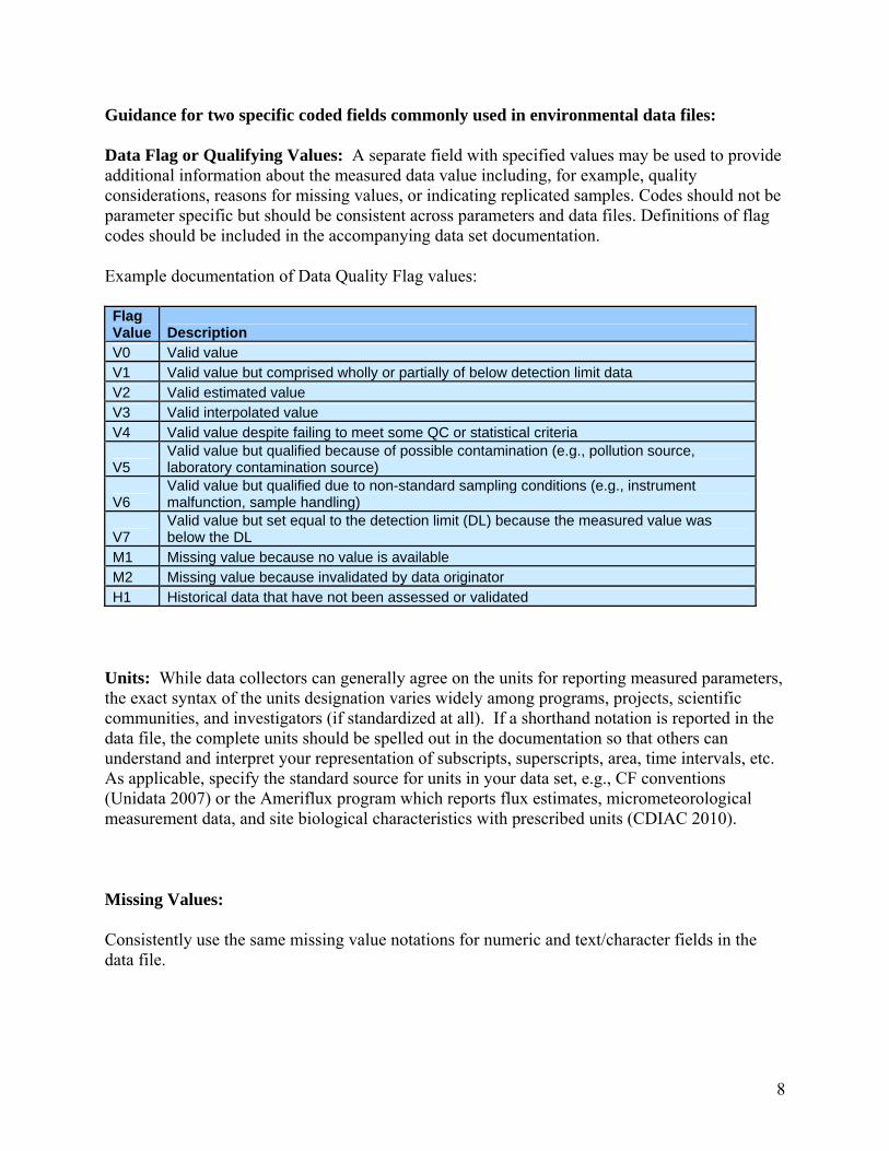
Guidance for two specific coded fields commonly used in environmental data files:

Data Flag or Qualifying Values: A separate field with specified values may be used to provide additional information about the measured data value including, for example, quality considerations, reasons for missing values, or indicating replicated samples. Codes should not be parameter specific but should be consistent across parameters and data files. Definitions of flag codes should be included in the accompanying data set documentation.

Example documentation of Data Quality Flag values:

Flag Value Description V0 Valid value V1 Valid value but comprised wholly or partially of below detection limit data V2 Valid estimated value V3 Valid interpolated value V4 Valid value despite failing to meet some QC or statistical criteria

V5 Valid value but qualified because of possible contamination (e.g., pollution source, laboratory contamination source)

V6 Valid value but qualified due to non-standard sampling conditions (e.g., instrument malfunction, sample handling)

V7 Valid value but set equal to the detection limit (DL) because the measured value was below the DL

M1 Missing value because no value is available M2 Missing value because invalidated by data originator H1 Historical data that have not been assessed or validated

Units: While data collectors can generally agree on the units for reporting measured parameters, the exact syntax of the units designation varies widely among programs, projects, scientific communities, and investigators (if standardized at all). If a shorthand notation is reported in the data file, the complete units should be spelled out in the documentation so that others can understand and interpret your representation of subscripts, superscripts, area, time intervals, etc. As applicable, specify the standard source for units in your data set, e.g., CF conventions (Unidata 2007) or the Ameriflux program which reports flux estimates, micrometeorological measurement data, and site biological characteristics with prescribed units (CDIAC 2010).

Missing Values:

Consistently use the same missing value notations for numeric and text/character fields in the data file.

8

9

For numeric fields: • You may use a specified extreme value not likely to ever be confused with the valid range of

a measured value (e.g., -9999). Representing missing data as a value outside the possible range of reasonable values will work for loading data into the widest range of programs.

• Alternatively, use a missing value code that matches the reporting format for the specific parameter. For example, use "-999.99", when the reporting format is a FORTRAN-like F7.2.

• In some cases, it may be appropriate to use the IEEE floating point NaN value (Not a Number) to represent missing data, particularly for floating point data columns that can assume any value. Likewise, the database “NULL” may be used in some instances. NULL value and NaN representations may be clearer, and are supported by many programs, but can cause some problems, particularly with older programs.

• Do not use character codes in an otherwise numeric field (except possibly for NULL or NaN to represent missing data) recognizing that this may cause processing problems for subsequent users.

• Document what the missing and nodata values represent. For character fields: • For character fields, it may be appropriate to use “NULL”, “Not applicable” or “None”

depending upon the organization of the data file. • For a text representation (e.g., a .csv file) it is better to use an explicit missing value

representation rather than two successive commas. Again, many applications will interpret two successive commas as a missing value, but other programs will create a mis-registration of the data (particularly older applications).

• It might be useful to use a placeholder value such as "Pending assignment" when compiling draft information to facilitate returning to incomplete fields.

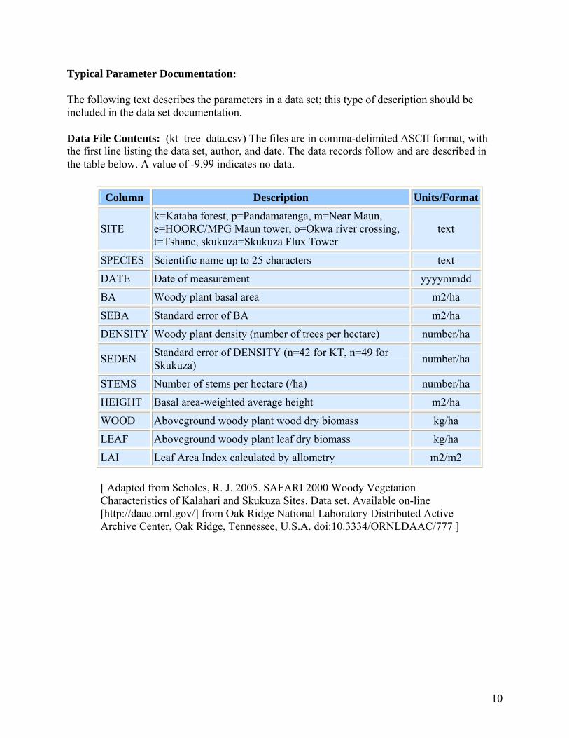
Typical Parameter Documentation:

The following text describes the parameters in a data set; this type of description should be included in the data set documentation.

Data File Contents: (kt_tree_data.csv) The files are in comma-delimited ASCII format, with the first line listing the data set, author, and date. The data records follow and are described in the table below. A value of -9.99 indicates no data.

Column Description Units/Format

SITE k=Kataba forest, p=Pandamatenga, m=Near Maun, e=HOORC/MPG Maun tower, o=Okwa river crossing, t=Tshane, skukuza=Skukuza Flux Tower

text

SPECIES Scientific name up to 25 characters text

DATE Date of measurement yyyymmdd

BA Woody plant basal area m2/ha

SEBA Standard error of BA m2/ha

DENSITY Woody plant density (number of trees per hectare) number/ha

SEDEN Standard error of DENSITY (n=42 for KT, n=49 for Skukuza) number/ha

STEMS Number of stems per hectare (/ha) number/ha

HEIGHT Basal area-weighted average height m2/ha

WOOD Aboveground woody plant wood dry biomass kg/ha

LEAF Aboveground woody plant leaf dry biomass kg/ha

LAI Leaf Area Index calculated by allometry m2/m2

[ Adapted from Scholes, R. J. 2005. SAFARI 2000 Woody Vegetation Characteristics of Kalahari and Skukuza Sites. Data set. Available on-line [http://daac.ornl.gov/] from Oak Ridge National Laboratory Distributed Active Archive Center, Oak Ridge, Tennessee, U.S.A. doi:10.3334/ORNLDAAC/777 ]

10

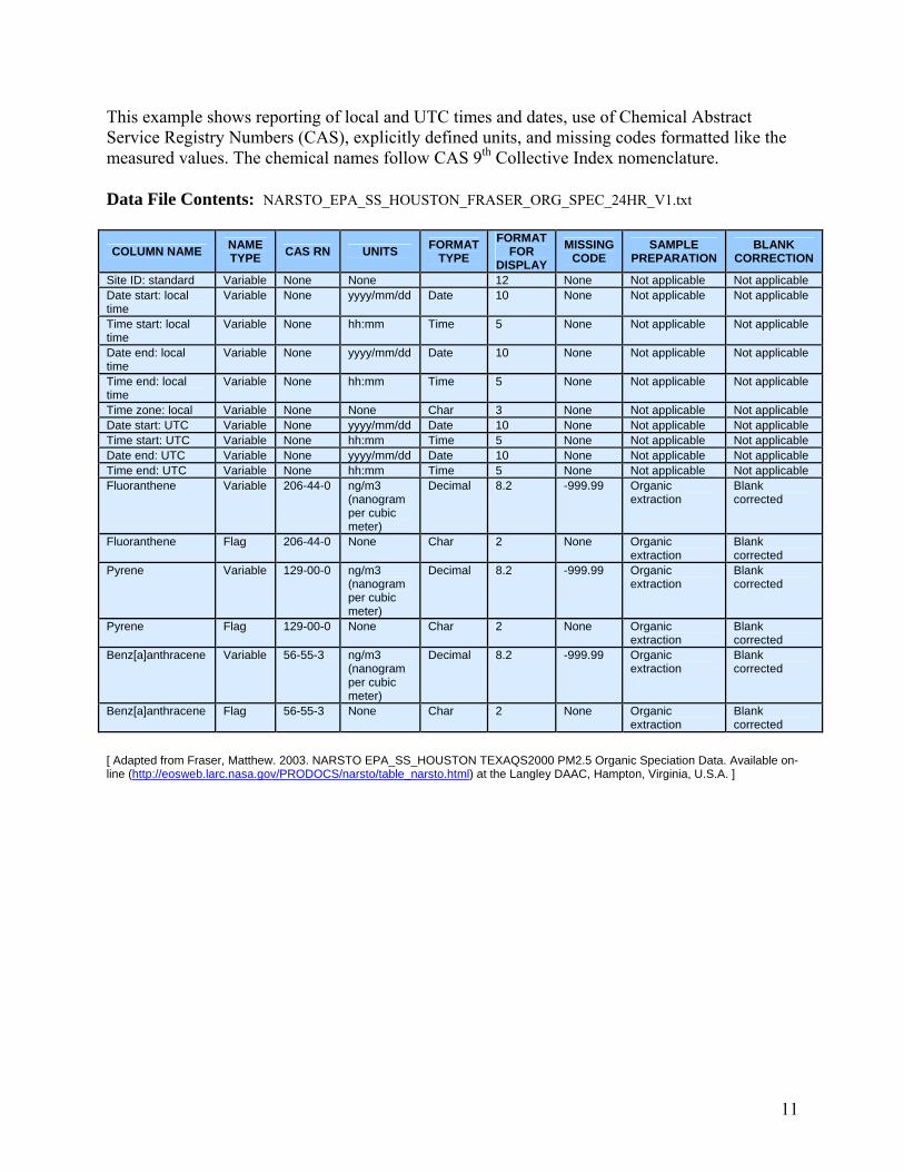
This example shows reporting of local and UTC times and dates, use of Chemical Abstract Service Registry Numbers (CAS), explicitly defined units, and missing codes formatted like the measured values. The chemical names follow CAS 9th Collective Index nomenclature.

Data File Contents: NARSTO_EPA_SS_HOUSTON_FRASER_ORG_SPEC_24HR_V1.txt

COLUMN NAME NAME TYPE CAS RN UNITS FORMAT

TYPE

FORMAT FOR

DISPLAY

MISSING CODE

SAMPLE PREPARATION

BLANK CORRECTION

Site ID: standard Variable None None 12 None Not applicable Not applicable Date start: local time

Variable None yyyy/mm/dd Date 10 None Not applicable Not applicable

Time start: local time

Variable None hh:mm Time 5 None Not applicable Not applicable

Date end: local time

Variable None yyyy/mm/dd Date 10 None Not applicable Not applicable

Time end: local time

Variable None hh:mm Time 5 None Not applicable Not applicable

Time zone: local Variable None None Char 3 None Not applicable Not applicable Date start: UTC Variable None yyyy/mm/dd Date 10 None Not applicable Not applicable Time start: UTC Variable None hh:mm Time 5 None Not applicable Not applicable Date end: UTC Variable None yyyy/mm/dd Date 10 None Not applicable Not applicable Time end: UTC Variable None hh:mm Time 5 None Not applicable Not applicable Fluoranthene Variable 206-44-0 ng/m3

(nanogram per cubic meter)

Decimal 8.2 -999.99 Organic extraction

Blank corrected

Fluoranthene Flag 206-44-0 None Char 2 None Organic extraction

Blank corrected

Pyrene Variable 129-00-0 ng/m3 (nanogram per cubic meter)

Decimal 8.2 -999.99 Organic extraction

Blank corrected

Pyrene Flag 129-00-0 None Char 2 None Organic extraction

Blank corrected

Benz[a]anthracene Variable 56-55-3 ng/m3 (nanogram per cubic meter)

Decimal 8.2 -999.99 Organic extraction

Blank corrected

Benz[a]anthracene Flag 56-55-3 None Char 2 None Organic extraction

Blank corrected

[ Adapted from Fraser, Matthew. 2003. NARSTO EPA_SS_HOUSTON TEXAQS2000 PM2.5 Organic Speciation Data. Available on-line (http://eosweb.larc.nasa.gov/PRODOCS/narsto/table_narsto.html) at the Langley DAAC, Hampton, Virginia, U.S.A. ]

11

2.2 Use Consistent Data Organization [ Return to Index ]

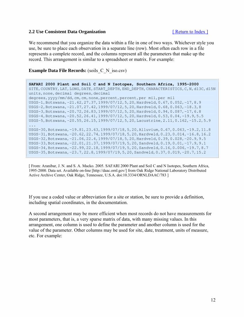
We recommend that you organize the data within a file in one of two ways. Whichever style you use, be sure to place each observation in a separate line (row). Most often each row in a file represents a complete record, and the columns represent all the parameters that make up the record. This arrangement is similar to a spreadsheet or matrix. For example:

Example Data File Records: (soils_C_N_iso.csv)

SAFARI 2000 Plant and Soil C and N Isotopes, Southern Africa, 1995-2000 SITE,COUNTRY,LAT,LONG,DATE,START_DEPTH,END_DEPTH,CHARACTERISTICS,C,N,d13C,d15Nunits,none,decimal degrees,decimal degrees,yyyy/mm/dd,cm,cm,none,percent,percent,per mil,per mil USGS-1,Botswana,-21.62,27.37,1999/07/12,5,20,Hardveld,0.67,0.052,-17,8.9 USGS-2,Botswana,-21.07,27.42,1999/07/12,5,20,Hardveld,0.68,0.063,-18.3,8 USGS-3,Botswana,-20.72,26.83,1999/07/12,5,20,Hardveld,0.94,0.087,-17,6.8 USGS-4,Botswana,-20.52,26.41,1999/07/12,5,20,Hardveld,0.53,0.04,-19.9,5.5 USGS-5,Botswana,-20.55,26.15,1999/07/12,5,20,Lacustrine,2.11,0.162,-15.2,5.9 ... USGS-30,Botswana,-19.81,23.63,1999/07/18,5,20,Alluvium,0.67,0.063,-19.2,11.8 USGS-31,Botswana,-20.62,22.74,1999/07/18,5,20,Hardveld,0.23,0.014,-16.8,16.2 USGS-32,Botswana,-21.06,22.4,1999/07/18,5,20,Hardveld,0.39,0.028,-20.9,9.5 USGS-33,Botswana,-22.01,21.37,1999/07/19,5,20,Sandveld,0.19,0.01,-17.9,9.1 USGS-34,Botswana,-22.99,22.18,1999/07/19,5,20,Sandveld,0.16,0.006,-19.7,8.7 USGS-35,Botswana,-23.7,22.8,1999/07/19,5,20,Sandveld,0.37,0.019,-20.7,15.2

[ From: Aranibar, J. N. and S. A. Macko. 2005. SAFARI 2000 Plant and Soil C and N Isotopes, Southern Africa, 1995-2000. Data set. Available on-line [http://daac.ornl.gov/] from Oak Ridge National Laboratory Distributed Active Archive Center, Oak Ridge, Tennessee, U.S.A. doi:10.3334/ORNLDAAC/783 ]

If you use a coded value or abbreviation for a site or station, be sure to provide a definition, including spatial coordinates, in the documentation.

A second arrangement may be more efficient when most records do not have measurements for most parameters, that is, a very sparse matrix of data, with many missing values. In this arrangement, one column is used to define the parameter and another column is used for the value of the parameter. Other columns may be used for site, date, treatment, units of measure, etc. For example:

12

Coast redwood NPP data from Humboldt Redwoods State Park, California, USA; Busing & Fujimori, June 2005 Old stand plot study at Bull Creek with bole diameter measurements at 1.7 m aboveground in 1972 and 2001 Orig_sort

_order Parameter Measurement

_Type Value Units Species Sequoia _sp_grav Equation

1 Latitude Site Characteristics 40.35 decimal degree Not applicable -999.9 Not applicable 2 Longitude Site Characteristics -123 decimal degree Not applicable -999.9 Not applicable 3 Terrain Site Characteristics Alluvial flat Not applicable Not applicable -999.9 Not applicable 4 Slope Site Characteristics 0 degree Not applicable -999.9 Not applicable

5

Elevation (above mean sea

level) Site Characteristics 80 m (meter) Not applicable -999.9 Not applicable 6 Total site area Site Characteristics 1.44 ha (hectare) Not applicable -999.9 Not applicable

7 Density Density 380 stems/ha

(stems per hectare) All species -999.9 Not applicable

8 Basal area Area 330

m2/ha (square meter per hectare) All species -999.9 Not applicable

9 Basal area Area 329

m2/ha (square meter per hectare) Sequoia -999.9 Not applicable

...

123 Total tree ANPP ANPP 581-697

g/m2/yr (gram per square

meter per year) All species 0.33 eq. 2 estimates

124 Total tree ANPP ANPP 669-802

g/m2/yr (gram per square

meter per year) All species 0.38 eq. 2 estimates

Sequoia_sp_grav: *Specific gravity, 0.33 mg/cm3, see WE Westman & RH Whittaker, 1975, J. Ecol. for details. Sequoia_sp_grav: ^Specific gravity, 0.38 mg/cm3, from DW Green et al., 1999, USDA Forest Service FPL-GTR-113. Method: **Calculations & allometric equations described by RT Busing & T Fujimori, 2005, Plant Ecol. Notes: ***Range of values results from min. & max. estimation ratios of WE Westman & RH Whittaker, 1975, J. Ecol.

From: Busing, R. T., and T. Fujimori. 2005. NPP Temperate Forest: Humboldt Redwoods State Park, California, U.S.A., 1972-2001. Data set. Available on-line [http://daac.ornl.gov] from Oak Ridge National Laboratory Distributed Active Archive Center, Oak Ridge, Tennessee, U.S.A. doi:10.3334/ORNLDAAC/803

Keep Similar Information Together An important issue with data organization is the number of records in each file (file size). There are a number of factors that determine the optimal number of records in a file, and we don't have any hard and fast rules. In general, keep a set of similar measurements together (e.g., same investigator, methods, time basis, and instruments) in one data file. Please do not break up your data into many small files, e.g., by month or by site if you are working with several months, years, or sites. Instead, make month or site a parameter and have all the data in one large file. Researchers who later use your relatively large data file won't have to process many small files individually. There is an upper limit to the size of files, though. Large files (on the order of several tens of thousands of records, or several tens of megabytes) do become unwieldy and may be too large

13

14

for some applications. For example, Excel 2003 will support 65,000 rows and 256 columns of data. Excel 2007 does not have these limitations. Large tabular data files may need to be broken into logical smaller files.

Organization by Data Type

If you are collecting many observations of several different types of measurements at a site (e.g., leaf area index and above- and belowground biomass), place each type of measurement in a separate data file. For each data file, use similar data organization, parameter formats, and common site names, so that users understand the interrelationships between data files.

Data types collected on different time bases (e.g., per hour, per day, per year) might be handled more efficiently in separate files.

Alternatively, if relatively few observations are made at a site for a suite of parameters, then all data could be placed in one file. Thorough data set documentation would be needed.

2.3 Use Consistent File Structure and Stable File Formats For Tabular and Image Data [ Return to Index ]

In choosing a file format, data collectors should select a consistent format that can be read well into the future and is independent of changes in applications. Excel, as an example, is a useful tool for data manipulations and data visualization, but versions of Excel files may become obsolete and may not be easily readable over the longer term. Likewise, database files can be a very effective way to store and manipulate data, but the raw formats tend to change over time (even a few years). If your collection operation has used proprietary file formats, creating an export in a stable, well-documented, and non-proprietary format is important for maximizing others’ abilities to use and build upon your data.

Tabular Data File Structure and Format:

Using delimited text file formats is the best way to ensure that measurement data are readable in the future.

• Use the same structure throughout the file - don't have a different number of columns or re-arrange the columns within the file.

• Use a consistent structure across all data files prepared for a study or project. • Figures and analyses should be reported in companion documents - don't place figures or

summary statistics in the data file. • ASCII American Standard Code for Information Interchange) is the most common text

encoding and the one most likely to be readable by tools. Other text encodings, such as UTF-8 are possible and may be necessary for some non-English applications. Avoid obscure text encodings. Use ASCII if possible, with UTF-8 or UTF-16 as secondary options.

At the top of the file, include several header rows:

• The first row should contain descriptors that link the data file to the data set, for example, the data file name, data set title, author, today's date, date the data within the file were last modified.

• Other header rows (column headings) should describe the content of each column, including one row for parameter names and one for parameter units.

• Column headings should be constructed for easy importing by various data systems. Headings should contain only numbers, letters, hyphens, and underscores -- no spaces or special characters. This also applies to column names and table names in databases. While many databases will allow spaces in table or column names, many do not and the use of spaces in table and column names causes the resulting SQL statements to be more difficult to read and more error-prone when editing is required.

Within the text file, follow these guidelines.

• Delimit the column headings and parameter fields using commas, tabs, semicolons, or vertical bars (|); these are listed in order of preference.

15

• Avoid delimiters that also occur in the data fields. If this cannot be avoided, enclose data fields that also contain a delimiter in single or double quotes.

• As noted above, do not use single or double quotes as part of a column name and avoid them in field values if at all possible.

• If the data fields use the comma as the decimal separator (rather than the period) the semicolon would be the preferred column delimiter.

• Use an explicit value for missing values, rather than an empty field. This is particularly important for tab delimited data files.

• Don't include rows with summary statistics; it is best to put summary statistics, figures, and other comments in a separate companion data file or in the data set documentation.

Use the data file extension that best indicates the type of file and field delimiters. For example, *.csv for comma-delimited text file and *.txt for a text file delimited with tabs or semicolons. Don't use *.dat since it has special meaning for PCs. See file extension reference, Appendix A.

In the data set documentation, specifically add the following data file information:

• Description of the data file names, particularly if the file names are composed of multiple acronyms, site abbreviations, or other project specific designations.

• Expanded descriptions of the parameters (column headings) and their units of measure from the data file.

• File delimiter. • Missing value codes. • Example data file records. • Other data file documentation, as listed in Best Practice 7, which would be helpful to a

secondary data user.

Image (Raster) Data File Format:

Some researchers may generate Image (Raster) data sets. Below are some guidelines / recommendations for archiving these types of data files.

Researchers should use non-proprietary file formats for storing their image data. Below are some suggested non-proprietary file formats:

• GeoTIFF/TIF (*.tiff, *.tif) • ESRI ASCII Grid (*.asc, *.txt) with detailed information on storage structure such as the

number of Columns, Rows, spatial resolution of the pixels, and projection information (*.prj)

• Binary Image files (BSQ/BIL/BIP) in (*.dat, *.bsq, *.bil) with detailed information on storage structure such as the number of Columns, Rows, Byte order (little endian or big endian), Data type (Float, Unsigned Integer, Double Precision, etc.), and Interleave defined in a companion header file (*.hdr).

• netCDF (CF convention)/netCDF – CF convention files (*.nc) • HDF-EOS / HDF (*.hdf)

16

If you have access to popular GIS packages, such as ENVI, ESRI ArcGIS, ERDAS IMAGINE, and IDRISI, make sure the image files can be opened readily using one of these software packages. Open source image readers, such as uDIG, GDAL and GRASS, can also be used to make sure the image files can be opened directly by these geospatial image readers.

If you cannot use any of the above formats, another option is to use any non-proprietary public domain data format. Whatever file format you use, be sure to thoroughly document the format and follow our suggested guidelines. Creating image files in a customized format that can only be used with your own FORTRAN or C program is strongly discouraged.

Geospatial Information for Image Files:

All image files should be supported with documentation describing all necessary geospatial information to correctly geolocate the images. Below is a list of required geospatial parameters:

• Definition of Projection/Coordinate reference system • Definition of the referenced Datum • EPSG code, if available • Spatial resolution of the data. If the resolution is different in X and Y direction, both

resolutions need to be provided. • Bounding Box – X, Y coordinates of the top-left/bottom-right pixels. While stating the

corner pixel coordinates, indicate if these coordinates lie within the center of the pixel or at one of the edges.

Note: There are multiple standards (e.g. OGC WKT (Open Geospatial Consortium Well-Known Text), ESRI WKT (Well-Known Text), and *.prj file) that can be used to define the projection/coordinate reference system and datum. A good reference site is http://spatialreference.org/.

If possible provide a companion header file with projection information. Example header files: ENVI, *.hdr file; TIF world file, *.tfw; ESRI projection file, *.prj.

Image files should be georeferenced prior to sending to the archive. File formats such as GeoTIFF that facilitate embedding the geospatial information inside the image file should be used where possible.

If this additional documentation is available provide it along with the geospatial information.

1. Rational for choosing a particular projection 2. Issues with reprojecting the data 3. Suggested resampling techniques (Nearest neighbor/Cubic convolution…etc) 4. Projection constraints

17

Storage Structure for Image Files:

• Store the image files in data types that fall within the valid range and type of the data contained in the image files. For example, if values of a parameter range from 1 to 100 and only have integer numbers, when it is stored in an image file, pick the BYTE data type for storing the data. This would ensure that the least amount of disk space is used while maintaining data integrity. Likewise pick signed integer/unsigned integer/float etc depending on the data range and type.

• Pick consistent and optimal NODATA values. Preferably 0 or -9999. Embed the NODATA values in the image files if possible. For example, GeoTIFF format allows the nodata values to be embedded in the file so software can automatically read the NODATA value and render the image accordingly.

• Document NODATA values; FILL Values, Valid ranges, scale factor and offset of the data values.

• Document what the nodata/fill values represent.

Additional considerations:

• If available provide a color look up table if available in the following format for the purpose to visualize the image file.

Red Green Blue Value 100 123 124 23 122 123 53 34 ………….

• Include pictures of binary image files so that a user can use them to check and to make sure that the binary images were read correctly. For example, include a *.jpg, *.png, *.gif, *.bmp, .tif, or .tiff pictures of geographic images

• Avoid using generic file extensions (e.g., *.bin or *.img). These extensions are used by many programs and could cause confusion on their origin. If the data are available in a generic format, explicitly state the software used to create/read the files.

• Provide information on what software package and version was used to create the data file(s). If the data files were created with custom code, provide a software program to enable the user to read the files (e.g., FORTRAN, C code, etc).

Proprietary Software Data Formats:

Data that are provided in a proprietary software format must include documentation of the software specifications (i.e., Software Package, Version, Vendor, and native platform). The archive data center will use this information to convert to a non-proprietary format for the archive.

18

19

Why follow these image recommendations:

1. Storing data in recommended formats with detailed documentation ensures data longevity. Using non-proprietary formats allows data to be easily read many years into the future

2. Storing the data using the recommendations listed above allows for the data to be readily exposed using interoperability standards such as OGC-Web Map service, Web Coverage Service. This increases data usage and allows one storage format but multiple distribution formats.

3. Users can spend more time analyzing the data and spend less time in data preparation. 4. Easy access means improved usability of the data in more researchers using and citing

your data.

Vector Data:

Below are suggested vector file formats. These are mostly proprietary data formats; please be sure to document the Software Package, Version, Vendor, and native platform.

• ARCVIEWsoftware -- we require *.shp, *.sbx, *.sbn, *.prj, and *.dbf files that contain the basic components of an ARCVIEW shape file. [ http://www.esri.com/ ]

• ENVI -- *.evf (ENVI vector file) [ http://www.rsinc.com/whoweare/index.asp ] • ESRI Arc/Info export file (.e00) [ http://www.esri.com/ ]

Also make sure that the vectors are properly geo-referenced and the geometry type (Point, Line, Polygon, Multipoint, etc) is specified. The requirements in the “Geospatial Information” section for Image Data also apply to Vector Data.

2.4 Assign Descriptive File Names [ Return to Index ]

File names should reflect the contents of the file and include enough information to uniquely identify the data file. File names may contain information such as project acronym, study title, location, investigator, year(s) of study, data type, version number, and file type. The file name should be provided in the documentation (described in Sect. 2.7) and in the first line of the header rows in the file itself.

Clear, descriptive, and unique file names may be important later when your data file is combined in a directory or FTP site with your own data files or with the data files of other investigators. Avoid using file names such as mydata.dat or 1998.dat.

File names should be constructed for easy management by various data systems. Names should contain only numbers, letters, dashes, and underscores -- no spaces or special characters. Also, in general, lower-case names are less software and platform dependent and are preferred. If you use mixed case file names (for readability), make sure that you do not have two filenames which differ only by case. When choosing a file name, check for any database management limitations on the use of special characters and file name length. For practical reasons of legibility and usability, file names should not be more than 64 characters in length and if well constructed could be considerably less.

You may want to use similar logic when designing directory structures and names. Also, the data set title (see Sect. 2.6) should be similar to the data file name(s).

Tabular Data File Naming Conventions:

Version Number: Including a data file creation date or version number enables data users to quickly determine which data they are using if an update to the data set is released (e.g., *_v1.csv, *_r1.csv, or *_20100615.csv).

File Type or Extensions: Use *.txt, *.csv generally for tabular data. Section 2.3 addresses formats and extensions for image data files.

If the Files are Compressed: Use *.zip, *.gz, or *.tar file extensions, as appropriate for the compression software. The individual files may be compressed for space conservation or several files may be aggregated and then compressed as one file of reduced size. When multiple files are compressed together, the same file naming guidelines apply to the compressed collection of files.

Example Data File Names:

• c130_a792_20000916.csv (From data set SAFARI 2000 C-130 Aerosol and Meteorological Data, Dry Season 2000)

• WBW_veg_inventory_all_20050304.csv (From data set Walker Branch Watershed Vegetation Inventory, 1967-1997)

20

• bigfoot_agro_2000_gpp.zip (From data set BigFoot GPP Surfaces for North and South American Sites, 2000-2004)

Image File Naming Convention:

Provide descriptive and consistent names to the image files. Below is a suggested pattern for the file names.

PPP_PARAM_STARTDATETIME_ENDDATETIME.file_extension

PPP- denotes a short word describing the image file/project.

PARAM- denotes the parameter stored in the image files. If multiple parameters are stored a universal descriptor of the parameters can be used. For example if soil characteristics such as soil type, soil moisture, soil clay content etc are all stored in the same image file, the parameter value can be stated as “soil”.

STARTDATETIME_ENDDATETIME denotes the start and end time of the data. This value represents the temporal range of the data quantity stored in the file. If the image file contains an observed value for a single date, a single time range can be provided.

The values of STARTDATETIME and ENDDATETIME should follow standard ISO 8601. See Appendix B. The format of the values is “YYYY-MM-DDThh:mm:ss.sTZD” (e.g. 1997-07-16T19:20:30.45+01:00), where:

YYYY = four-digit year MM = two-digit month (01=January, etc.) DD = two-digit day of month (01 through 31) hh = two digits of hour (00 through 23) (am/pm NOT allowed) mm = two digits of minute (00 through 59) ss = two digits of second (00 through 59) s = one or more digits representing a decimal fraction of a second TZD = time zone designator (Z or +hh:mm or -hh:mm)

Not all parts of the datetime value need to be provided. For example, if only year and month are available, simply use format “YYYY-MM”.

File_extension – Is the file extension of the image file. The following files use .tif, .nc, .tif, and .bil formats.

LBA_leafarea_20091001_20100101.tif BOREAS_soils_20091001.nc MODIS_landcover-IGBP_2001.tif Global_carbonflux-2001_2006.bil

21

22

2.5 Perform Basic Quality Assurance [ Return to Index ]

In addition to scientific quality assurance (QA), we suggest that you perform basic data QA on the data files prior to sharing. These checks complement the Tabular and Image file preparation guidance provided in Section 2.3. When QA is finished, describe the overall quality level of the data.

QA for Tabular Data

• Check file structure by making sure the data are delimited/line up in the proper columns. • Check file organization and descriptors to ensure that there are no missing values for key

parameters (such as sample identifier, station, time, date, geographic coordinates). Sort the records by key data fields to highlight discrepancies.

• Review the documentation to ensure that descriptions accurately reflect the data file names, format, and content. Check any included example data records to ensure that they are from the latest version of the data file.

• Check the content of measured or derived values. Scan parameters for impossible values (e.g., pH of 74 or negative values where negative values are not possible). Review printed copies of the data file(s) and generate time series plots to detect anomalous values or data gaps.

• Perform statistical summaries (frequency of parameter occurrence) and review results. • If location is a parameter (latitude/longitude), then use scatter plots or GIS software to

map each location to see if there are any errors in coordinates. • Verify data transfers (from field notebooks, data loggers, or instruments). For data

transformations done by hand, consider double data entry (entering data twice, comparing the two data sets, and reconciling any differences). Where possible compare summary statistics before and after data transformation.

• To document changes between versions of tabular data files consider using available "file difference applications". See Appendix E.

• Calculate checksums for final data files and include verification files along with the data files when transferred to the data archive. See Appendix E for checksum calculation and verification applications.

QA for Image Vector and Raster Data

For GIS image/vector files, ensure that the projection parameters have been accurately given. Additional information such as data type, scale, corner coordinates, missing data value, size of image, number of bands, endian type should be checked for accuracy.

• File Size o For binary data, are the n(rows) *[ n(cols) * n(bands) * (bytes per pixel)] = files

size? o Provide checksum files to ensure data integrity during network transfer. o Do not perform file compression unless file sizes are very large (Consult with the

data archive on acceptable file sizes.).

• Data Format o Is the data in the format indicated by the file extension and documentation? o Is the data readable in standard GIS/Image processing software (e.g., ENVI, Erdas

IMAGINE, or ArcGIS)? o Data format specific issues:

Is the header information accurate for binary files? Are ASCII file values expressed as plain numbers (e.g.,0.000222, not

scientific notation)? o For multi band images, are the number of bands in the data equal to that specified

in the documentation? o Additional documentation required for data format, i.e., the file is not self-

documenting. • Georeferencing Information

o Projection Is projection information provided? If provided, is it correct? (check with other accurately projected data) Are the projection parameters such as Central meridian, datum, standard

parallels, radius of earth (If different from standard) provided? If the projection is a non-standard projection is a projection file provided

in .prj or Well-Known Text (WKT) format. Does the projection render within a GIS software package such as

ENVI/ArcGIS. o Spatial extent

Does the data extent match the documentation? Does the data extent match the number of pixels and resolution of the

data? What are the units (degrees/meters) of the extents provided? In what projection are the extents provided. Provide the extents of the data file and not the extent of the study area

contained within the data file. In some cases the image files might include additional area.

o Spatial resolution Is the resolution specified? What are the resolution units (meters, feet, decimal degrees etc.) correct?

• Specify How the Data are to be Read o Does the data range match that given in the documentation? o Does the data read from upper left to lower right or lower left to upper right or

any other way? o What is/are the nodata value(s)? o What is the scale of the data? o Are their any data offsets? o What are the units of the data? o Is there a color table that can be used with the data? If so provide the color table

in “Value, Red, Green, Blue” format.

23

• Temporal Resolution o Is the data provided for the time frame specified in the documentation? o Are the temporal units correct?

Define the Quality of Your Data Users want to quickly understand the overall quality of your data and the analyses and processing steps that may have been applied to your data and image products. This information can be included in a data file as coded values (e.g., Level 2) and as a more complete description in metadata and documentation. The quality description should identify the level of maturity of your data products as they progress from raw data streams, to products that have undergone automated quality control, data management procedures, and calibration, to data that have been integrated, analyzed, and gridded, and lastly, products that have been derived for other products and used in models and higher level analyses. Here are some guidelines for defining the quality of tabular and image products that you are preparing to share. Tabular Data Quality Typically, measurement data for sharing and archiving are at Quality Level 2 following this general progression.

• Level 0: Indicates products of unspecified quality that have been subjected to minimal processing in the field and/or in the laboratory (e.g., raw data, data sheets, etc.). This may, for example, be data from an instrument logger expressed in engineering units or using nominal calibrations, or high resolution data before aggregating to a selected interval.

• Level 1: Indicates an internally consistent data product that has been subjected to quality checks and data management procedures.

• Level 2: Indicates a complete, externally consistent data product that has undergone interpretative and diagnostic analysis.

• Level 3: Data that have received intense scrutiny through analysis or use in modeling. Another good approach is being implemented by the National Ecological Observatory Network (NEON) (http://www.neoninc.org/): Definition of Data Product Quality Levels for NEON.

• Level 0: Raw data from instrumental or human observations. • Level 1: Calibrated data generally from a single instrument, observer, or field sampling

area. These data may include information on data quality. • Level 2: Combinations of level 1 data used to create a gap filled data stream that may

replace a level 1 product. Generally, products at this level will reflect a stream from a single instrument, observer, or field sampling area. Annotations will indicate the gap filling approach employed.

• Level 3: Level 1 and /or 2 data mapped on a uniform space-time grid. • Level 4: Derived products using levels 1, 2 or 3 data. Products at this level may combine

observations from more than one instrument, observer, or sampling area.

24

25

For additional information see the NEON Data Product Catalogs (http://www.neoninc.org/documents/513). Image Vector and Raster Data Quality There is no generally applicable standard for defining and expressing the processing and quality level of image products. Quality level should be specified in documentation and could use some of the same terminology as in the example below. If a product is derived from a source that has defined processing levels, such as the MODIS instrument (https://lpdaac.usgs.gov/lpdaac/products/modis_overview), then that information should be included. Following is a set of generally applicable processing levels (http://outreach.eos.nasa.gov/EOSDIS_CD-03/docs/proc_levels.htm). Processing Level

• Level 0: Reconstructed, unprocessed data at full resolution; all communications artifacts have been removed

• Level 1: Level 0 data that has been time-referenced and annotated with ancillary information, including radiometric and geometric calibration coefficients, and geolocation information

• Level 2: Derived geophysical variables at the same resolution and location as the Level 1 data

• Level 3: Variables mapped on uniform space-time grids, usually with some completeness and consistency

• Level 4: Model output or results from analyses of lower level data

2.6 Assign Descriptive Data Set Titles [ Return to Index ]

We recommend that data set titles be as descriptive as possible. The title may be the first thing people will see when looking at a dataset. So making descriptive titles is important for people searching for data. When giving titles to your data sets and associated documentation, please be aware that these data sets may be accessed many years in the future by people who will be unaware of the details of the project.

Data set titles should contain the type of data and other information such as the date range, the location, and the instruments used. If your data set is part of a larger field project, you may want to add that name, too (e.g., SAFARI 2000 or LBA-ECO). In addition, we recommend that the length of the title be restricted to 85 characters (spaces included) to be compatible with other clearinghouses of ecological and global change data collections. Names should contain only numbers, letters, dashes, underscores, periods, commas, colons, parentheses, and spaces -- no special characters. The data set title should be similar to the name(s) of the data file(s) in the data set (see Sect. 2.4). A given data set might contain only one data file or many thousands of data files.

Some bad titles:

• "The Aerostar 100 Data Set" • "Respiration Data"

Some great titles:

• "SAFARI 2000 Upper Air Meteorological Profiles, Skukuza, Dry Seasons 1999-2000"

• "LBA-ECO CD-07 GOES-8 L3 Gridded Surface Radiation and Rain Rate for Amazonia: 1999"

• "Global Fire Emissions Database, Version 2 (GFEDv2.2)" • LBA-ECO ND-11 Ecotone Vegetation Survey and Biomass, NW Mato Grosso,

Brazil: 2004 • LBA-ECO LC-24 AVHRR Derived Fire Occurrence, 5-km Resolution, Amazonia

2001

26

2.7 Provide Data Set Documentation and Metadata [ Return to Index ]

In order for your data to be identified, found, accessed, and used properly by others in the future, they must be thoroughly documented. The documentation accompanying your data set should be written for a user 20 years into the future. Therefore, you should consider what that investigator needs to know to use your data. Write the documentation for a user who is unfamiliar with your project, sites, methods, or observations.

A subset of the documentation, the fields that concisely identify the "who, what, where, when, and why" of the data, are referred to as metadata or "data about the data". These consistently formatted fields serve as the basis for searchable metadata databases and clearinghouses to facilitate the discovery of your data set by the scientific community and public. A list of typical discovery metadata is included in Appendix F. Several metadata standards have been developed to ensure compatibility and interoperability across databases and clearinghouses, including FGDC (FGDC 2010), NetCDF Attribute Convention for Dataset Discovery (Unidata 2005), Ecological Metadata Language (EML) (KNB 2010), and ISO-19115 (ISO 2009). The standard for metadata implemented by the archive for your data should be identified and values for any standard-specific fields should be provided.

Documentation Format: To ensure that documentation can be read well into the future requires that it be in a stable non-proprietary format. If figures, maps, equations, or pictures need to be included, use a non-proprietary document format such as html (hypertext markup language). Images, figures, and pictures may be included as individual gif (graphics interchange format) or jpg (Joint Photographic Experts Group) files. Converting documents to a stable proprietary format, such as Adobe pdf (portable document format) files, is a good choice. The documentation should be in a separate file that is identified in the data file. The name of the documentation file should be similar to the name of the data set and the data file(s). From the data user's perspective, the document is most useful when structured as a user's guide to the data product. Documentation Content: The data set documentation should provide the following information:

• The name of the data set, which will be the title of the documentation (see Sect. 2.6) • What data were collected • The scientific reason why the data were collected • Who funded the investigation • Who collected the data and who to contact with questions (include e-mail and Web

address if appropriate) • How to cite the data set (Appendix G) • When and how frequently the data were collected

27

• Where and with what spatial resolution the data were collected. • If codes are used for location, be sure to define the codes in the documentation. • The name(s) of the data file(s) in the data set (see Sect. 2.4) • Special codes used, including those for missing values (see Sect. 2.1) or for stations (see

Sect. 2.2) • The date the data set was last modified • The English language translation of any data values and descriptors that are in another

language (e.g., coded fields, variable classes, and GIS coverage attributes). • Parameter descriptions as shown in the examples above (see Sect. 2.1) • Example data file records for each data type file • How each parameter was measured or produced (methods), its units of measure, the

format used for the parameters in the data set, the precision and accuracy if known, and the relationship to other data in the data set if appropriate (see Sect. 2.1)

• What instruments (including model and serial number) (e.g., rain gauge) and source (meteorological station) were used

• Standards or calibrations that were used • What the environmental conditions were (e.g., cloud cover, atmospheric influences, etc.) • The data processing that was performed, including screening • The lineage (provenance) of the data (Islam, 2010) • Software (including version number) used to prepare the data set • Software (including version number) needed to read the data set • The quality assurance and quality control that have been applied (see Sect. 2.5) • Describe the quality level of the data • Known problems that limit the data's use (e.g., uncertainty, sampling problems, blanks,

QC samples) • Summary statistics generated directly from the final data file for use in verifying file

transfer and transformations. • Pertinent field notes or other companion files; the names of the files should be similar to

the documentation and data file names • Related or ancillary data sets • References to published papers describing the collection and/or analysis of the data

Documentation can never be too complete. The amount and scope of metadata and data documentation needed to accompany data increases when users are not familiar with the data collection activities, i.e., the public, and even over the lifetime of long-term experimental activities.

Creating Archive Metadata and Documentation

The discovery (finding and accessing) of data sets by the scientific community and public is facilitated through the compilation of metadata records and their inclusion into searchable metadata databases and clearinghouses. The ORNL DAAC's Advanced Data Search (i.e., Mercury, http://mercury.ornl.gov/ornldaac/index.jsp?tab=advanced) is one example. Others include NASA's Global Change Master Directory (GCMD) (http://gcmd.gsfc.nasa.gov) and NASA’s Warehouse Inventory Search Tool (WIST) (https://wist.echo.nasa.gov/api/) data clearinghouses.

28

These search applications may have preferred data file formats (e.g., NetCDF) and additional metadata requirements. Metadata standards including FGDC, NetCDF Attribute Convention for Dataset Discovery, EML, and ISO-19115 may be the preferred standard and need be considered when making decisions about the metadata elements to collect and document. Metadata entry and management tools are integrated with most metadata databases to ensure that required metadata are provided and consistently formatted. Most entry tools and databases also export metadata in formats to meet multiple standards and provide for interoperability between metadata search clearinghouses. Examples of metadata entry tools include the ORNL DAAC's Online Metadata Editor (OME) (https://daac.ornl.gov/cgi-bin/MDE/RGED/access.pl), Metavist 2 (http://metavist2.codeplex.com/), and Ecological Metadata Language (EML) (http://knb.ecoinformatics.org/morphoportal.jsp).

29

3 Bibliography

ANU 2008. ANU Data Management Manual: Managing Digital Research Data at the Australian National University. http://ilp.anu.edu.au/dm/ANU_DM_Manual_v1.03.pdf Ball, C. A., G. Sherlock, and A. Brazma. 2004. Funding high-throughput data sharing. Nature Biotechnology 22:1179-1183. doi:10.1038/nbt0904-1179. Barton, C., R. Smith and R. Weaver . 2010. Data Practices, Policy, and Rewards in the Information Era Demand a New Paradigm. Data Science Journal. IGY95-IGY99. Borer, Elizabeth T., Eric W. Seabloom, Matthew B. Jones, and Mark Schildhauer. 2009. Some Simple Guidelines for Effective Data Management. Bulletin of the Ecological Society of America. 90:205—214. [doi:10.1890/0012-9623-90.2.205] Carbon Dioxide Information Analysis Center (CDIAC). 2010. AmeriFlux Network Data Submission Guidelines. http://public.ornl.gov/ameriflux/data-guidelines.shtml . Christensen, S. W. and L. A. Hook. 2007. NARSTO Data and Metadata Reporting Guidance. Provides reference tables of chemical, physical, and metadata variable names for atmospheric measurements. Available on-line at: http://cdiac.ornl.gov/programs/NARSTO/ Cook, R.B., et al., 2010. The 95th ESA Annual Meeting, Workshop 13 - How to Prepare Ecological Data Sets for Effective Analysis and Sharing. http://eco.confex.com/eco/2010/techprogram/S5744.HTM Cook, Robert B, Richard J. Olson, Paul Kanciruk, and Leslie A. Hook. 2001. Best Practices for Preparing Ecological Data Sets to Share and Archive. Bulletin of the Ecological Society of America, Vol. 82, No. 2, April 2001. DDI. 2010. Data Documentation Initiative (DDI) - A metadata specification for the social sciences. http://www.ddialliance.org/ Accessed 20100830. Digital Curation Centre (DCC). 2010. DMP online - The DCC Data Management Planning Tool. http://eidcsr.blogspot.com/2010/05/digital-curation-centre-has-developed.html , September 1, 2010. Federal Geographic Data Committee (FGDC) 2010. The North American Profile (NAP) of the ISO 19115. http://www.fgdc.gov/metadata/geospatial-metadata-standards Higgins, Sarah (2008), The DCC Curation Lifecycle Model, The International Journal of Digital Curation Issue 1, Volume 3, 2008, pp 134-140

30

Islam, Sidra. 2010. Provenance, Lineage, and Workflows. Master Thesis. Computer Science Department, Brown University, RI, USA. http://www.cs.brown.edu/research/pubs/theses/masters/2010/islam.pdf International Organization for Standardization (ISO). 2009. ISO 19115-2:2009, Geographic information -- Metadata -- Part 2: Extensions for imagery and gridded data. http://www.iso.org/iso/catalogue_detail.htm?csnumber=39229 Inter-university Consortium for Political and Social Research (ICPSR). (2009). Guide to Social Science Data Preparation and Archiving: Best Practice Throughout the Data Life Cycle (4th ed.). Ann Arbor, MI. Karasti, H. and Baker, K.S. "Digital Data Practices and the Long Term Ecological Research Program Growing Global." International Journal of Digital Curation. Vol. 3, No.2, (2008) http://www.ijdc.net/ijdc/article/view/86/104 Knowledge Network for Biocomplexity (KNB). 2010. Ecological Metadata Language (EML) http://knb.ecoinformatics.org/software/eml/. Kanciruk, P., R.J. Olson, and R.A. McCord. 1986. Quality Control in Research Databases: The US Environmental Protection Agency National Surface Water Survey Experience. In: W.K. Michener (ed.). Research Data Management in the Ecological Sciences. The Belle W. Baruch Library in Marine Science, No. 16, 193-207. Michener, W. K., J. W. Brunt, J. Helly, T. B. Kirchner, and S. G. Stafford. 1997. Non-Geospatial Metadata for Ecology. Ecological Applications. 7:330-342. Michener, W.K. and J.W. Brunt (ed.). 2000. Ecological Data: Design, Management and Processing, Methods in Ecology, Blackwell Science. 180p. Michener, W K. 2006. Meta-information concepts for ecological data management. Ecological Informatics. 1:3-7. MIT Libraries. 2010. Data Management and Publishing, Massachusetts Institute of Technology. http://libraries.mit.edu/guides/subjects/data-management/index.html . Accessed 20100830. National Science Foundation. 2010. Scientists Seeking NSF Funding Will Soon Be Required to Submit Data Management Plans. http://www.nsf.gov/news/news_summ.jsp?cntn_id=116928&org=NSF. Press Release 10-077, May 10, 2010. Olsen, L.M., G. Major, K. Shein, J. Scialdone, R. Vogel, S. Leicester, H. Weir, S. Ritz, T. Stevens, M. Meaux, C.Solomon, R. Bilodeau, M. Holland, T. Northcutt, and R. A. Restrepo. 2007. NASA/Global Change Master Directory (GCMD) Earth Science Keywords. Version 6.0.0.0.0. Available on-line at: http://gcmd.gsfc.nasa.gov/Resources/valids/archives/keyword_list.html

31

Science Environment for Ecological Knowledge (SEEK) 2007. Introduction to Ecoinformatics. http://seek.ecoinformatics.org/Wiki.jsp?page=SEEKPostdoctoralAndNewFacultyTrainingJanuary8122007 Thornton, P.E., R.B. Cook, B.H. Braswell, B.E. Law, W. M. Post, H. H. Shugart, B.T. Rhyne, and L.A. Hook. 2005. Archiving Numerical Models of Biogeochemical Dynamics. Eos, Vol. 86, No. 44, 1 November 2005. UK Data Archive. 2010. The Data Lifecycle. http://www.data-archive.ac.uk/home. Accessed 20100830. UK Data Archive. 2009. Managing and Sharing Data: a best practice guide for researchers. www.data-archive.ac.uk/sharing Unidata. 2005. NetCDF Attribute Convention for Dataset Discovery. http://www.unidata.ucar.edu/software/netcdf-java/formats/DataDiscoveryAttConvention.html Unidata. 2007. NetCDF (network Common Data Form) with CF (Climate and Forecast) Conventions - Units. Accessed August 2010. http://www.unidata.ucar.edu/projects/THREDDS/GALEON/netCDFprofile-short.htm . U.S. EPA. 2007. Environmental Protection Agency Substance Registry System (SRS). SRS provides information on substances and organisms and how they are represented in the EPA information systems. Available on-line at: http://www.epa.gov/srs/ USGS. 2000. Metadata in plain language. Available on-line at: http://geology.usgs.gov/tools/metadata/tools/doc/ctc/

32

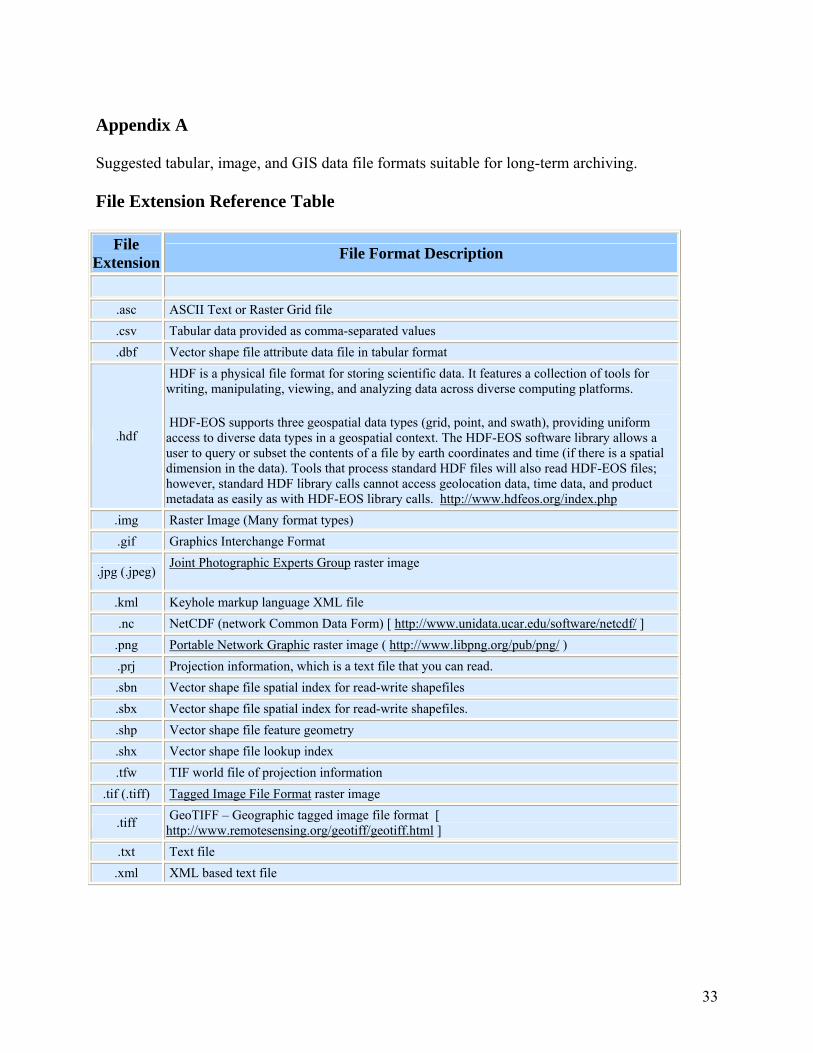
Appendix A

Suggested tabular, image, and GIS data file formats suitable for long-term archiving.

File Extension Reference Table

File Extension File Format Description

.asc ASCII Text or Raster Grid file .csv Tabular data provided as comma-separated values .dbf Vector shape file attribute data file in tabular format

.hdf

HDF is a physical file format for storing scientific data. It features a collection of tools for writing, manipulating, viewing, and analyzing data across diverse computing platforms. HDF-EOS supports three geospatial data types (grid, point, and swath), providing uniform access to diverse data types in a geospatial context. The HDF-EOS software library allows a user to query or subset the contents of a file by earth coordinates and time (if there is a spatial dimension in the data). Tools that process standard HDF files will also read HDF-EOS files; however, standard HDF library calls cannot access geolocation data, time data, and product metadata as easily as with HDF-EOS library calls. http://www.hdfeos.org/index.php

.img Raster Image (Many format types) .gif Graphics Interchange Format

.jpg (.jpeg) Joint Photographic Experts Group raster image

.kml Keyhole markup language XML file .nc NetCDF (network Common Data Form) [ http://www.unidata.ucar.edu/software/netcdf/ ]

.png Portable Network Graphic raster image ( http://www.libpng.org/pub/png/ ) .prj Projection information, which is a text file that you can read. .sbn Vector shape file spatial index for read-write shapefiles .sbx Vector shape file spatial index for read-write shapefiles. .shp Vector shape file feature geometry .shx Vector shape file lookup index .tfw TIF world file of projection information

.tif (.tiff) Tagged Image File Format raster image

.tiff GeoTIFF – Geographic tagged image file format [ http://www.remotesensing.org/geotiff/geotiff.html ]

.txt Text file .xml XML based text file

33

Appendix B

Applicable data and time standards suitable for long-term archiving of environmental data.

Applicable Date and Time Standards

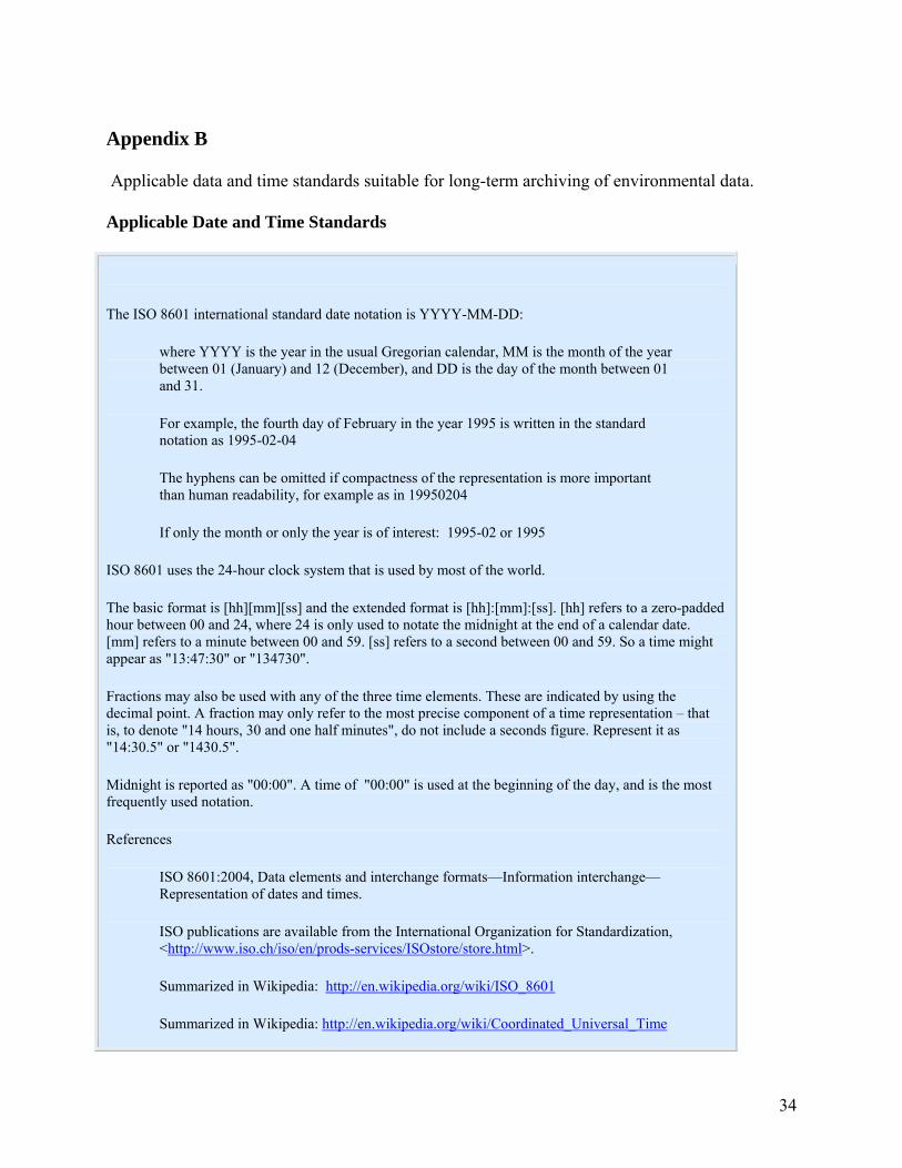
The ISO 8601 international standard date notation is YYYY-MM-DD:

where YYYY is the year in the usual Gregorian calendar, MM is the month of the year between 01 (January) and 12 (December), and DD is the day of the month between 01 and 31.

For example, the fourth day of February in the year 1995 is written in the standard notation as 1995-02-04

The hyphens can be omitted if compactness of the representation is more important than human readability, for example as in 19950204

If only the month or only the year is of interest: 1995-02 or 1995

ISO 8601 uses the 24-hour clock system that is used by most of the world.

The basic format is [hh][mm][ss] and the extended format is [hh]:[mm]:[ss]. [hh] refers to a zero-padded hour between 00 and 24, where 24 is only used to notate the midnight at the end of a calendar date. [mm] refers to a minute between 00 and 59. [ss] refers to a second between 00 and 59. So a time might appear as "13:47:30" or "134730".

Fractions may also be used with any of the three time elements. These are indicated by using the decimal point. A fraction may only refer to the most precise component of a time representation – that is, to denote "14 hours, 30 and one half minutes", do not include a seconds figure. Represent it as "14:30.5" or "1430.5".

Midnight is reported as "00:00". A time of "00:00" is used at the beginning of the day, and is the most frequently used notation.

References

ISO 8601:2004, Data elements and interchange formats—Information interchange—Representation of dates and times.

ISO publications are available from the International Organization for Standardization, <http://www.iso.ch/iso/en/prods-services/ISOstore/store.html>.

Summarized in Wikipedia: http://en.wikipedia.org/wiki/ISO_8601

Summarized in Wikipedia: http://en.wikipedia.org/wiki/Coordinated_Universal_Time

34

Appendix C

Applicable spatial coordinate standards suitable for long-term archiving of image and GIS data.

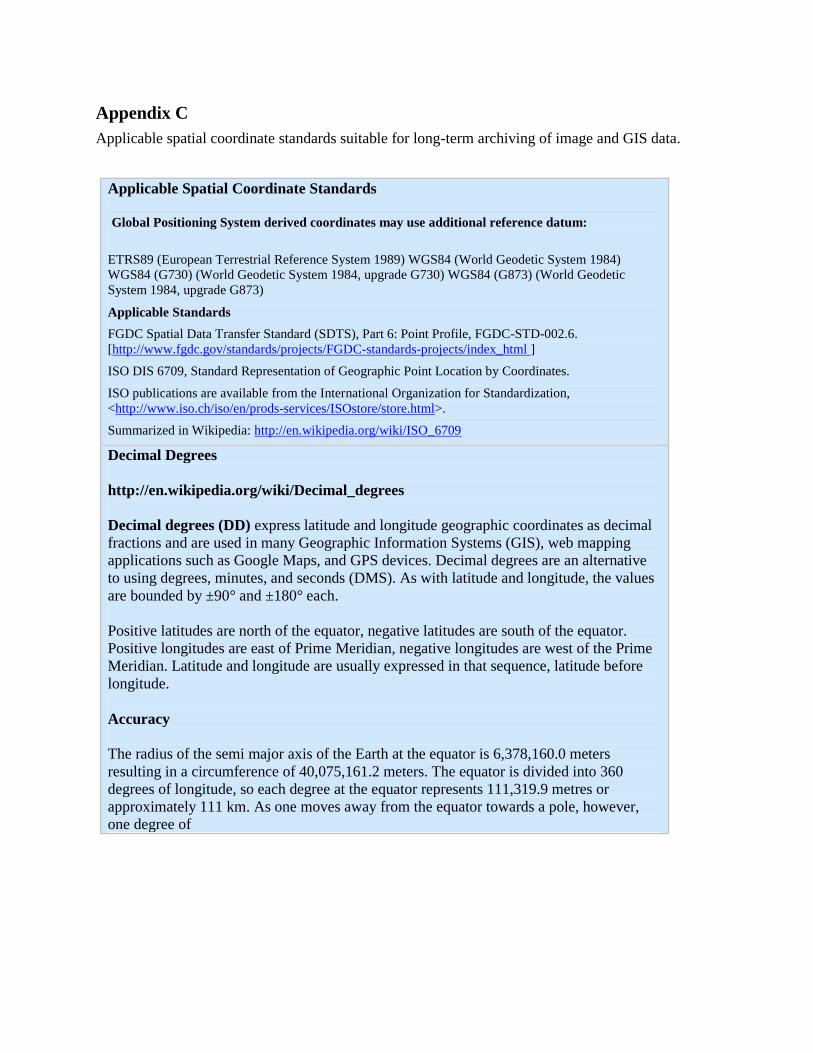
Applicable Spatial Coordinate Standards

Global Positioning System derived coordinates may use additional reference datum:

ETRS89 (European Terrestrial Reference System 1989) WGS84 (World Geodetic System 1984)

WGS84 (G730) (World Geodetic System 1984, upgrade G730) WGS84 (G873) (World Geodetic

System 1984, upgrade G873)

Applicable Standards

FGDC Spatial Data Transfer Standard (SDTS), Part 6: Point Profile, FGDC-STD-002.6.

[http://www.fgdc.gov/standards/projects/FGDC-standards-projects/index_html ]

ISO DIS 6709, Standard Representation of Geographic Point Location by Coordinates.

ISO publications are available from the International Organization for Standardization,

<http://www.iso.ch/iso/en/prods-services/ISOstore/store.html>.

Summarized in Wikipedia: http://en.wikipedia.org/wiki/ISO_6709

Decimal Degrees

http://en.wikipedia.org/wiki/Decimal_degrees

Decimal degrees (DD) express latitude and longitude geographic coordinates as decimal

fractions and are used in many Geographic Information Systems (GIS), web mapping

applications such as Google Maps, and GPS devices. Decimal degrees are an alternative

to using degrees, minutes, and seconds (DMS). As with latitude and longitude, the values

are bounded by ±90° and ±180° each.

Positive latitudes are north of the equator, negative latitudes are south of the equator.

Positive longitudes are east of Prime Meridian, negative longitudes are west of the Prime

Meridian. Latitude and longitude are usually expressed in that sequence, latitude before

longitude.

Accuracy

The radius of the semi major axis of the Earth at the equator is 6,378,160.0 meters

resulting in a circumference of 40,075,161.2 meters. The equator is divided into 360

degrees of longitude, so each degree at the equator represents 111,319.9 metres or

approximately 111 km. As one moves away from the equator towards a pole, however,

one degree of

longitude represents a diminishing number of meters, approaching zero at the pole.

The length of a degree of longitude and the number of decimal places required for a

particular accuracy at the equator are:

Accuracy versus decimal places

decimal

places

degrees distance

0 1.0 111 km

1 0.1 11.1 km

2 0.01 1.11 km

3 0.001 111 m

4 0.0001 11.1 m

5 0.00001 1.11 m

6 0.000001 0.111 m

7 0.0000001 1.11 cm

8 0.00000001 1.11 mm

A value in decimal degrees to an accuracy of 4 decimal places is accurate to 11.1 meters

(+/- 5.55 m) at the equator. A value in decimal degrees to 5 decimal places is accurate to

1.11 meter at the equator. Because the earth is a spheroid and not flat, the accuracy of the

longitude part of the coordinates increases the further from the equator you get. The

accuracy of the latitude part does not increase.

Calculate the length of a degree of longitude and the number of decimal places

required for a particular accuracy at your specific latitude.

http://www.csgnetwork.com/degreelenllavcalc.html

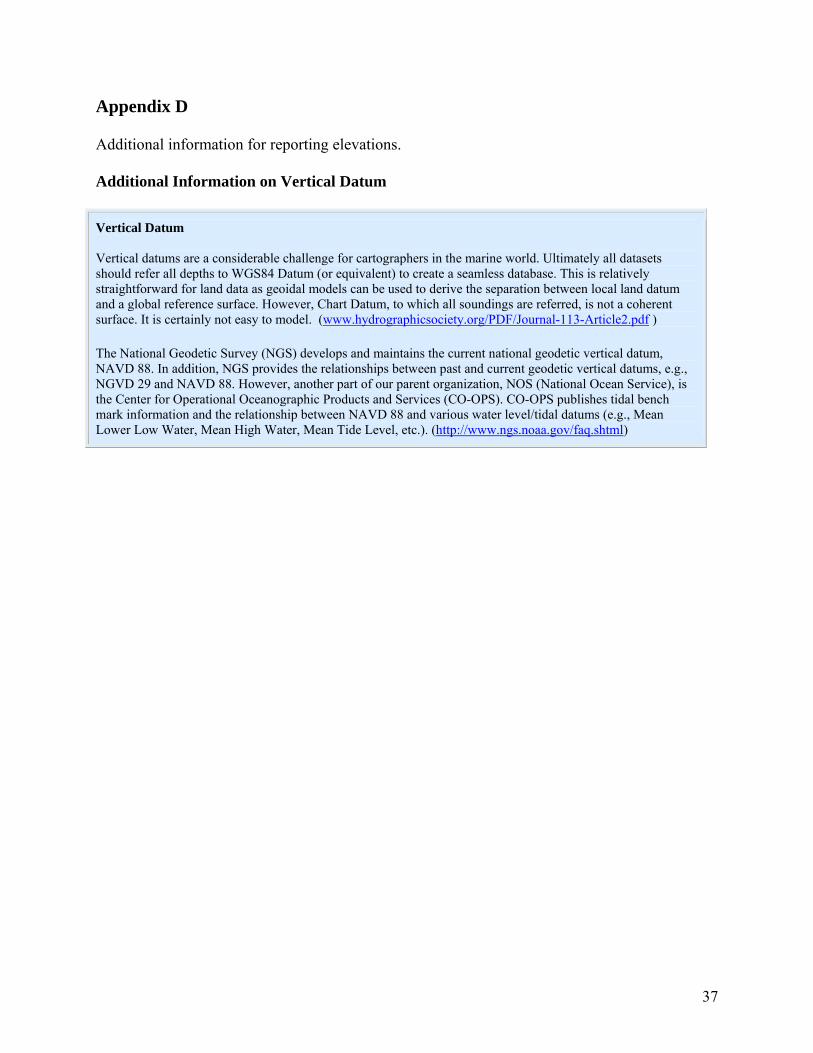
Appendix D

Additional information for reporting elevations.

Additional Information on Vertical Datum

Vertical Datum Vertical datums are a considerable challenge for cartographers in the marine world. Ultimately all datasets should refer all depths to WGS84 Datum (or equivalent) to create a seamless database. This is relatively straightforward for land data as geoidal models can be used to derive the separation between local land datum and a global reference surface. However, Chart Datum, to which all soundings are referred, is not a coherent surface. It is certainly not easy to model. (www.hydrographicsociety.org/PDF/Journal-113-Article2.pdf )

The National Geodetic Survey (NGS) develops and maintains the current national geodetic vertical datum, NAVD 88. In addition, NGS provides the relationships between past and current geodetic vertical datums, e.g., NGVD 29 and NAVD 88. However, another part of our parent organization, NOS (National Ocean Service), is the Center for Operational Oceanographic Products and Services (CO-OPS). CO-OPS publishes tidal bench mark information and the relationship between NAVD 88 and various water level/tidal datums (e.g., Mean Lower Low Water, Mean High Water, Mean Tide Level, etc.). (http://www.ngs.noaa.gov/faq.shtml)

37

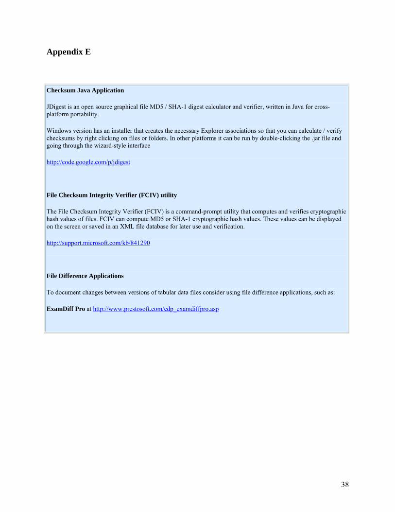
Appendix E

Checksum Java Application

JDigest is an open source graphical file MD5 / SHA-1 digest calculator and verifier, written in Java for cross-platform portability.

Windows version has an installer that creates the necessary Explorer associations so that you can calculate / verify checksums by right clicking on files or folders. In other platforms it can be run by double-clicking the .jar file and going through the wizard-style interface

http://code.google.com/p/jdigest

File Checksum Integrity Verifier (FCIV) utility

The File Checksum Integrity Verifier (FCIV) is a command-prompt utility that computes and verifies cryptographic hash values of files. FCIV can compute MD5 or SHA-1 cryptographic hash values. These values can be displayed on the screen or saved in an XML file database for later use and verification.

http://support.microsoft.com/kb/841290

File Difference Applications

To document changes between versions of tabular data files consider using file difference applications, such as:

ExamDiff Pro at http://www.prestosoft.com/edp_examdiffpro.asp

38

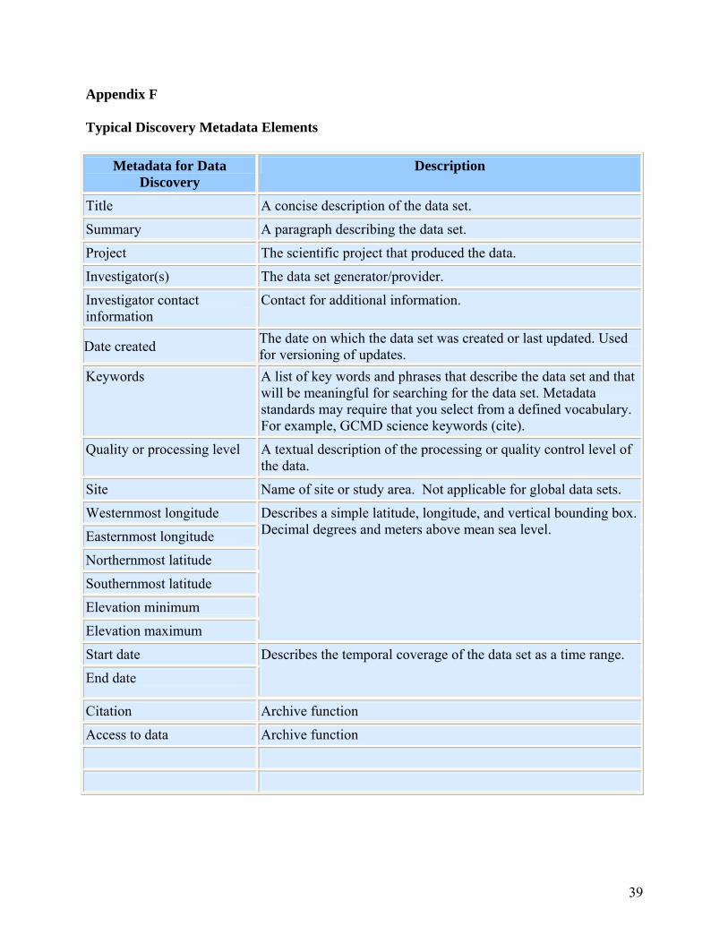
Appendix F

Typical Discovery Metadata Elements

Metadata for Data Discovery

Description

Title A concise description of the data set.

Summary A paragraph describing the data set.

Project The scientific project that produced the data.

Investigator(s) The data set generator/provider.

Investigator contact information

Contact for additional information.

Date created The date on which the data set was created or last updated. Used for versioning of updates.

Keywords A list of key words and phrases that describe the data set and that will be meaningful for searching for the data set. Metadata standards may require that you select from a defined vocabulary. For example, GCMD science keywords (cite).

Quality or processing level A textual description of the processing or quality control level of the data.

Site Name of site or study area. Not applicable for global data sets.

Westernmost longitude

Easternmost longitude

Northernmost latitude

Southernmost latitude

Elevation minimum

Elevation maximum

Describes a simple latitude, longitude, and vertical bounding box. Decimal degrees and meters above mean sea level.

Start date

End date

Describes the temporal coverage of the data set as a time range.

Citation Archive function

Access to data Archive function

39

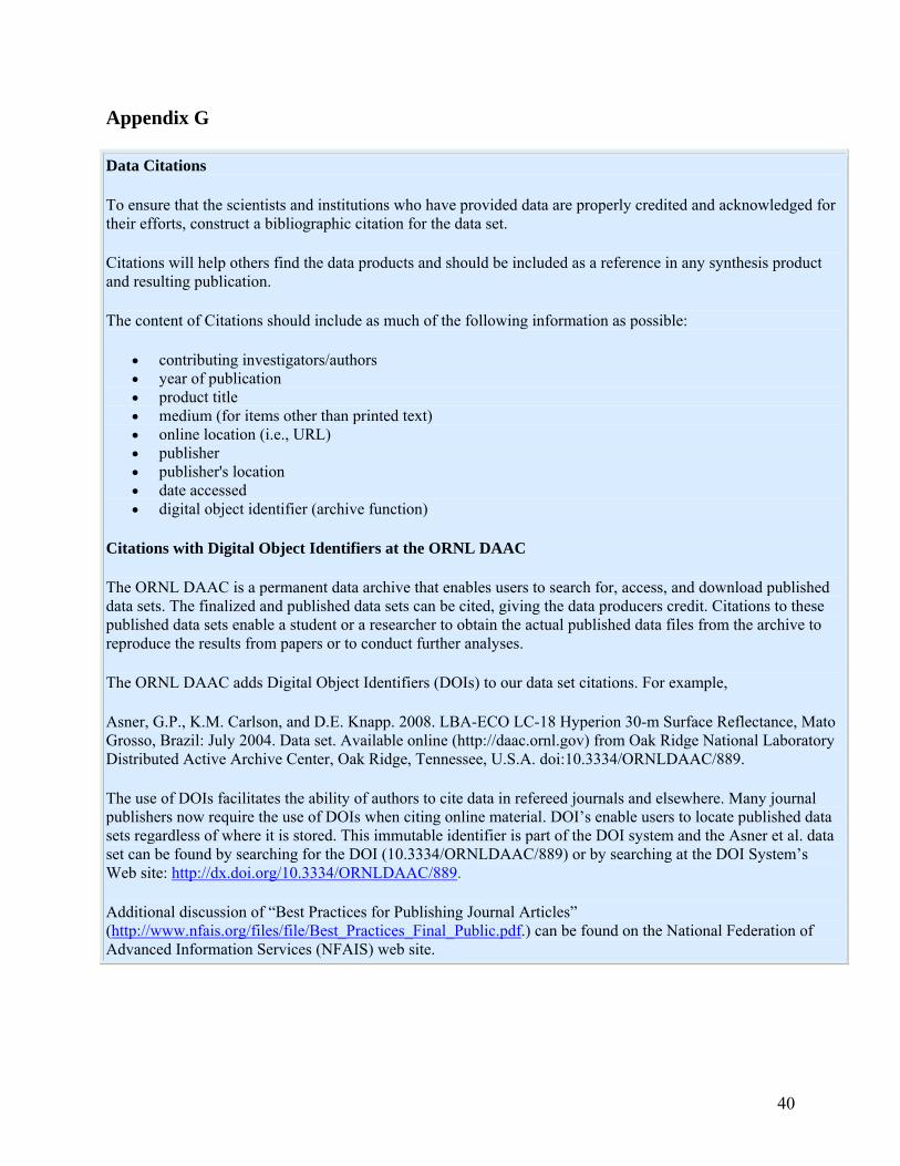
40

Appendix G

Data Citations

To ensure that the scientists and institutions who have provided data are properly credited and acknowledged for their efforts, construct a bibliographic citation for the data set.

Citations will help others find the data products and should be included as a reference in any synthesis product and resulting publication.

The content of Citations should include as much of the following information as possible:

• contributing investigators/authors • year of publication • product title • medium (for items other than printed text) • online location (i.e., URL) • publisher • publisher's location • date accessed • digital object identifier (archive function)

Citations with Digital Object Identifiers at the ORNL DAAC

The ORNL DAAC is a permanent data archive that enables users to search for, access, and download published data sets. The finalized and published data sets can be cited, giving the data producers credit. Citations to these published data sets enable a student or a researcher to obtain the actual published data files from the archive to reproduce the results from papers or to conduct further analyses.

The ORNL DAAC adds Digital Object Identifiers (DOIs) to our data set citations. For example,

Asner, G.P., K.M. Carlson, and D.E. Knapp. 2008. LBA-ECO LC-18 Hyperion 30-m Surface Reflectance, Mato Grosso, Brazil: July 2004. Data set. Available online (http://daac.ornl.gov) from Oak Ridge National Laboratory Distributed Active Archive Center, Oak Ridge, Tennessee, U.S.A. doi:10.3334/ORNLDAAC/889.

The use of DOIs facilitates the ability of authors to cite data in refereed journals and elsewhere. Many journal publishers now require the use of DOIs when citing online material. DOI’s enable users to locate published data sets regardless of where it is stored. This immutable identifier is part of the DOI system and the Asner et al. data set can be found by searching for the DOI (10.3334/ORNLDAAC/889) or by searching at the DOI System’s Web site: http://dx.doi.org/10.3334/ORNLDAAC/889.

Additional discussion of “Best Practices for Publishing Journal Articles” (http://www.nfais.org/files/file/Best_Practices_Final_Public.pdf.) can be found on the National Federation of Advanced Information Services (NFAIS) web site.