benjamin recht - peoplebrecht/papers/recht.thesis.pdf · convex modeling with priors by benjamin...
TRANSCRIPT

Convex Modeling with Priors
by
Benjamin Recht
B.S., University of Chicago (2000)M.S., Massachusetts Institute of Technology (2002)
Submitted to the Media Arts and Sciencesin partial fulfillment of the requirements for the degree of
Doctor of Philosophy
at the
MASSACHUSETTS INSTITUTE OF TECHNOLOGY
June 2006
c© Massachusetts Institute of Technology 2006. All rights reserved.
Author . . . . . . . . . . . . . . . . . . . . . . . . . . . . . . . . . . . . . . . . . . . . . . . . . . . . . . . . . . . . . .Media Arts and Sciences
April 14, 2006
Certified by. . . . . . . . . . . . . . . . . . . . . . . . . . . . . . . . . . . . . . . . . . . . . . . . . . . . . . . . . .Neil Gershenfeld
Associate ProfessorThesis Supervisor
Accepted by . . . . . . . . . . . . . . . . . . . . . . . . . . . . . . . . . . . . . . . . . . . . . . . . . . . . . . . . .Andrew B. Lippman
Chairman, Departmental Committee on Graduate Students

2

Convex Modeling with Priors
by
Benjamin Recht
Submitted to the Media Arts and Scienceson April 14, 2006, in partial fulfillment of the
requirements for the degree ofDoctor of Philosophy
Abstract
As the study of complex interconnected networks becomes widespread across disciplines,modeling the large-scale behavior of these systems becomes both increasingly importantand increasingly difficult. In particular, it is of tantamount importance to utilize availableprior information about the system’s structure when building data-driven models of complexbehavior. This thesis provides a framework for building models that incorporate domainspecific knowledge and glean information from unlabelled data points.
I present a methodology to augment standard methods in statistical regression withpriors. These priors might include how the output series should behave or the specifics ofthe functional form relating inputs to outputs. My approach is optimization driven: by for-mulating a concise set of goals and constraints, approximate models may be systematicallyderived. The resulting approximations are convex and thus have only global minima andcan be solved efficiently. The functional relationships amongst data are given as sums ofnonlinear kernels that are expressive enough to approximate any mapping. Depending onthe specifics of the prior, different estimation algorithms can be derived, and relationshipsbetween various types of data can be discovered using surprisingly few examples.
The utility of this approach is demonstrated through three exemplary embodiments.When the output is constrained to be discrete, a powerful set of algorithms for semi-supervised classification and segmentation result. When the output is constrained to followMarkovian dynamics, techniques for nonlinear dimensionality reduction and system identi-fication are derived. Finally, when the output is constrained to be zero on a given set andnon-zero everywhere else, a new algorithm for learning latent constraints in high-dimensionaldata is recovered.
I apply the algorithms derived from this framework to a varied set of domains. Thedissertation provides a new interpretation of the so-called Spectral Clustering algorithmsfor data segmentation and suggests how they may be improved. I demonstrate the tasks oftracking RFID tags from signal strength measurements, recovering the pose of rigid objects,deformable bodies, and articulated bodies from video sequences. Lastly, I discuss empiricalmethods to detect conserved quantities and learn constraints defining data sets.
Thesis Supervisor: Neil GershenfeldTitle: Associate Professor
3

4

Convex Modeling with Priors
by
Benjamin Recht
PhD Thesis
Signature Page
Thesis Advisor. . . . . . . . . . . . . . . . . . . . . . . . . . . . . . . . . . . . . . . . . . . . . . . . . . . . . . . . . . . . . . . . . . . . .
Neil Gershenfeld
Associate Professor
Department of Media Arts and Sciences
Massachusetts Institute of Technology
Thesis Reader . . . . . . . . . . . . . . . . . . . . . . . . . . . . . . . . . . . . . . . . . . . . . . . . . . . . . . . . . . . . . . . . . . . . .
John Doyle
John G. Braun Professor
Departments of Control and Dynamical Systems, Electrical Engineering, and
BioEngineering
California Institute of Technology
Thesis Reader . . . . . . . . . . . . . . . . . . . . . . . . . . . . . . . . . . . . . . . . . . . . . . . . . . . . . . . . . . . . . . . . . . . . .
Pablo Parrilo
Associate Professor
Department of Electrical Engineering and Computer Science
Massachusetts Institute of Technology
5

6

Acknowledgments
I would first like to thank the members of my committee for providing invaluable guidanceand support. My advisor, Neil Gershenfeld, encouraged me to pursue my diverse interestsand provided a stimulating environment in which to do so. John Doyle took me under hiswing and introduced me to the wide world of robustness. Pablo Parrilo shared his manyinsights and creative suggestions on this document and on the score of papers we still haveleft in the queue.
The work in this thesis arose out of a long-running collaboration with Ali Rahimi.Most of the results contained herein are distilled from papers we have written togetheror ideas composed in late nights of brainstorming and coding (with some bickering). I’dlike to thank him for such a fruitful collaboration. This document benefited from a carefulreading by Ryan Rifkin who provided many useful comments and corrections. Aram Harrowsuggested a simple proof of Theorem 4.2.4. Along with being my co-conspirator on theAudiopad project, James Patten provided the hardware and his time for the acquisition ofthe Sensetable data in Chapter 5. Andy Sun and Jon Santiago assisted in the collection ofthe Resistofish data also discussed in Chapter 5. Kenneth Brown, Bill Butera, ConstantineCaramanis, Waleed Farahat, Tad Hirsch, and Dan Paluska also provided helpful feedback.
I’d especially like to thank Raffaello D’Andrea for his friendship and mentorship duringmy graduate career. I’d like to thank everyone else I have collaborated with during my stayat MIT including Ethan Bordeaux, Isaac Chuang, Brian Chow, Chris Csikszentmihalyi,Trevor Darrell, Saul Griffith and Squid Labs, Hiroshii Ishii, Seth Lloyd, Yael Maguire,Cameron Marlow, Jim McBride, Ryan McKinley, Ravi Pappu, Jason Taylor, Noah Vawter,Brian Whitman, and the students of the MIT Media Lab. I have learned more in thesecollaborations with my peers than anywhere else in my graduate career. I would also liketo acknowledge my other fellow travellers in the Physics and Media Group: Rich F., AraK., Raffi K., Femi O., Rehmi P., Manu P., Matt R., Amy S., and Ben V.
None of this work would have been possible without the diligent staff of the CBA office.I’d like to thank Susan Murphy-Bottari, Kelly Maenpaa, and Mike Houlihan for all of theirhelp, hard work, and support. I also extend my gratitude to Linda Peterson and Pat Solakoffin the MAS office for making it easier to leap over the hurdles that accompany the graduateschool process.
My involvment in the Boston electronic music scene has served as an important coun-terpoint to and release from my academic work. Notable shout outs go to The Fun Years,The Dan Bensons Project, Mike Uzzi, The Saltmine, Unlockedgroove, The DSP MusicSyndicate, The Appliance of Science, non-event, Beat Research, Spectrum, Jake Trussell,Anthony Flackett, Collision, Don Mennerich, Eric Gunther, Fred Giannelli, and StewartWalker. We are the reason Boston is the drone capital of the universe.
Of course, I am deeply indebted to Mom and Dad for their endless support. I’d like tothank my sister Marissa for putting up with my bad attitude longer than any reasonableperson would have. And finally, I’d like to thank Lauren, without whom I would haveprobably finished this thesis, but it wouldn’t have been half as good.
This work was supported in part by the Center for Bits and Atoms (NSF CCR-0122419),ARDA/DTO (F30602-30-2-0090), and the MITRE Corporation (0705N7KZ-PB).
7

8
Contents
1 Introduction 21
1.1 Contributions and Organization . . . . . . . . . . . . . . . . . . . . . 23
1.2 Notation . . . . . . . . . . . . . . . . . . . . . . . . . . . . . . . . . . 24
2 Mathematical Background 27
2.1 Basics of Convexity . . . . . . . . . . . . . . . . . . . . . . . . . . . . 27
2.1.1 Convex Sets . . . . . . . . . . . . . . . . . . . . . . . . . . . . 27
2.1.2 Convex Functions . . . . . . . . . . . . . . . . . . . . . . . . . 28
2.1.3 Convex Optimization . . . . . . . . . . . . . . . . . . . . . . . 31
2.2 Convex Relaxations . . . . . . . . . . . . . . . . . . . . . . . . . . . . 34
2.2.1 Nonconvex Quadratically Constrained Quadratic Programming 36
2.2.2 Applications in Combinatorial Optimization . . . . . . . . . . 40
2.3 Reproducing Kernel Hilbert Spaces and Regularization Networks . . . 47
2.3.1 Lessons from Linear Regression . . . . . . . . . . . . . . . . . 49
2.3.2 Reproducing Kernel Hilbert Spaces . . . . . . . . . . . . . . . 51
2.3.3 The Kernel Trick and Nonlinear Regression . . . . . . . . . . 53
3 Augmenting Regression with Priors 57
3.1 Duality and the Representer Theorem . . . . . . . . . . . . . . . . . . 58
3.2 Augmenting Regression with Priors on the Output . . . . . . . . . . . 63
3.2.1 Least-Squares Cost . . . . . . . . . . . . . . . . . . . . . . . . 64
3.2.2 The Need for Constraints . . . . . . . . . . . . . . . . . . . . 66
3.2.3 Priors on the Output . . . . . . . . . . . . . . . . . . . . . . . 68
9

3.2.4 Semi-supervised and Unsupervised Learning . . . . . . . . . . 71
3.3 Augmenting Regression with Priors on Functional Form . . . . . . . . 72
3.3.1 The Dual of the Arbitrary Regularization Problem . . . . . . 73
3.3.2 A Decomposition Algorithm for Solving the Dual Problem and
Kernel Learning . . . . . . . . . . . . . . . . . . . . . . . . . . 75
3.3.3 Example 1: Finite Set of Kernels . . . . . . . . . . . . . . . . 76
3.3.4 Example 2: Gaussian Kernels . . . . . . . . . . . . . . . . . . 78
3.3.5 Example 3: Polynomial Kernels . . . . . . . . . . . . . . . . . 80
3.4 Conclusion . . . . . . . . . . . . . . . . . . . . . . . . . . . . . . . . . 83
4 Output Prior: Binary Labels 85
4.1 Transduction, Clustering, and Segmentation via constrained outputs . 87
4.2 RKHS Clustering is NP-HARD . . . . . . . . . . . . . . . . . . . . . 90
4.3 Semidefinite Approximation using Lagrangian Duality . . . . . . . . . 94
4.4 Eigenvalue Approximations and the Normalized Cuts Algorithm . . . 98
4.4.1 The Normalized Cuts Algorithm . . . . . . . . . . . . . . . . . 99
4.4.2 Average Gap Algorithm . . . . . . . . . . . . . . . . . . . . . 101
4.5 Numerical Experiments . . . . . . . . . . . . . . . . . . . . . . . . . . 103
4.6 Conclusion . . . . . . . . . . . . . . . . . . . . . . . . . . . . . . . . . 105
5 Output Prior: Dynamics 107
5.1 Related Work . . . . . . . . . . . . . . . . . . . . . . . . . . . . . . . 108
5.2 Model for Semi-Supervised Nonlinear System ID . . . . . . . . . . . . 110
5.2.1 Semi-supervised Algorithm . . . . . . . . . . . . . . . . . . . . 115
5.2.2 Unsupervised Algorithm . . . . . . . . . . . . . . . . . . . . . 117
5.3 Relation to System Identification . . . . . . . . . . . . . . . . . . . . 118
5.4 Interactive Tracking Experiments . . . . . . . . . . . . . . . . . . . . 119
5.4.1 The Dynamics Model . . . . . . . . . . . . . . . . . . . . . . . 120
5.4.2 Synthetic Results . . . . . . . . . . . . . . . . . . . . . . . . . 120
5.4.3 Interactive Tracking . . . . . . . . . . . . . . . . . . . . . . . 123
5.4.4 Calibration of HCI Devices . . . . . . . . . . . . . . . . . . . . 124
10

5.4.5 Electric Field Imaging: . . . . . . . . . . . . . . . . . . . . . . 129
5.5 Conclusion . . . . . . . . . . . . . . . . . . . . . . . . . . . . . . . . . 131
6 Output Prior: Manifolds of Low Codimension 135
6.1 Learning Manifolds of Low Codimension . . . . . . . . . . . . . . . . 136
6.2 Basis Functions and Polynomial Models . . . . . . . . . . . . . . . . . 137
6.3 Lifting to a General RKHS . . . . . . . . . . . . . . . . . . . . . . . . 138
6.4 Null Spaces and Learning Surfaces . . . . . . . . . . . . . . . . . . . 139
6.5 Choosing a Basis . . . . . . . . . . . . . . . . . . . . . . . . . . . . . 141
6.6 Learning Manifolds . . . . . . . . . . . . . . . . . . . . . . . . . . . . 141
7 Conclusion 145
A Linear Algebra 149
A.1 Unconstrained Quadratic Programming . . . . . . . . . . . . . . . . . 149
A.2 Schur Complements . . . . . . . . . . . . . . . . . . . . . . . . . . . . 150
A.3 More Quadratic Programming . . . . . . . . . . . . . . . . . . . . . . 150
A.4 Inverting Partitioned Matrices . . . . . . . . . . . . . . . . . . . . . . 151
A.5 Schur complement Lemma . . . . . . . . . . . . . . . . . . . . . . . . 151
A.6 Matrix Inversion Lemma . . . . . . . . . . . . . . . . . . . . . . . . . 152
A.7 Lemmas on Matrix Borders . . . . . . . . . . . . . . . . . . . . . . . 152
B Equality Constrained Norm Minimization on an Arbitrary Inner
Product Space 155
11

12

List of Figures
2-1 Left and Middle: Two convex sets. In each set a line segment is drawn
between two points in the set and this line never leaves the set. Right:
A nonconvex set. Two points are shown which cannot be connected by a
straight line that doesn’t leave the set. . . . . . . . . . . . . . . . . . . . 28
2-2 Left: A convex function. One can readily check that the area above the
blue curve contains all line segments between all points. Right: The red
segment demonstrates that the region above the graph is not convex. . . . 30
2-3 The convex set is separated from the points not in the set by half-spaces.
The bold dashed line separates the plane into two halves, one containing
the point x and the other containing the convex set. . . . . . . . . . . . . 31
2-4 The set of possible pairs of g(x) and f(x) are shown as the blue region. Left:
Any hyperplane which has normal (µ, 1) intersects the y-axis at the point
f(x∗) + µ>g(x∗) where x∗ minimizes L(x, µ) with respect to x. Middle:
A hyperplane whose y intercept is equal to the minimum of f(x) on the
feasible set. The dual optimal value is equal to that of the primal Right: No
hyperplane can achieve the primal optimal value. The discrepancy between
the primal and dual optima is called a duality gap. The dual optimum value
is always a lower bound for the primal. . . . . . . . . . . . . . . . . . . 34
2-5 Left: Given four point, a variety of exact fits are shown. A prior on the
function is required to make the problem well-posed. Right: Regularization
Networks place a “bump” at each observed data point to fit unseen data. . 47
13

4-1 In Normalized Cuts, an outlier can dwarf the influence of other points,
because points away from the mean are heavily weighted. Sliding the outlier
(indicated by the arrow) along the x-axis can shift the clustering boundary
arbitrarily to the left or the right. Without the outlier, Normalized Cuts
places the boundary between the two clusters. . . . . . . . . . . . . . . . 102
4-2 Because Normalized Cuts puts more weight on points away from the mean,
it prefers to have the ends of the elongated vertical cluster on opposite sides
of the separating hyperplane. . . . . . . . . . . . . . . . . . . . . . . . . 102
4-3 The data set of Figure 4-1 is correctly segmented by weighting all points
equally. The outlier point doesn’t shift the clustering boundary significantly. 104
4-4 The data set of Figure 4-2 is correctly segmented by weighting all points
equally. . . . . . . . . . . . . . . . . . . . . . . . . . . . . . . . . . . . 104
5-1 A generative model for a linear system with nonlinear output. The states st
are low-dimensional representations lifted to high dimensional observables
xt by an embedding g. . . . . . . . . . . . . . . . . . . . . . . . . . . . 118
5-2 Forcing agreement between projections of observed xt and a Markov chain
of states st. The function f maps observations to outputs of a linear system. 119
5-3 The covariance between samples over time for various (A,C) pairs. The
x-axis represents number of samples from −1500 to 1500. The y-axis shows
covariance on a relative scale from 0 to 1. (top-left) Newtonian dynamics
model used in the experiments. (top-right) Dynamics model using zero ac-
celeration. (bottom-left) Brownian Motion model. (bottom-right) A second
order model with oscillatory modes. . . . . . . . . . . . . . . . . . . . . 121
14

5-4 (top-left) The true 2D parameter trajectory. Semi-supervised points are
marked with big black triangles. The trajectory is sampled at 1500 points
(small markers). Points are colored according to their y-coordinate on the
manifold. (top-middle) Embedding of a path via the lifting F (x, y) =
(x, |y|, sin(πy)(y2 + 1)−2 + 0.3y). (top-right) Recovered low-dimensional
representation using our algorithm. The original data in (top-left) is cor-
rectly recovered. (bottom-left) Even sampling of the rectangle [0, 5]×[−3, 3].
(bottom-middle) Lifting of this rectangle via F . (bottom-right) Projection
of (bottom-middle) via the learned function g. g has correctly learned the
mapping from 3D to 2D. These figures are best viewed in color. . . . . . 122
5-5 (left) Isomap’s projection into R2 of the data set of Figure 5-4(top-middle).
Errors in estimating the neighborhood relations at the neck of the manifold
cause the projection to fold over itself. (right) Projection with BNR, a semi-
supervised regression algorithm. There is no folding, but the projections are
not close to the ground truth shown in Figure 5-4(top-left). . . . . . . . . 122
5-6 The bounding box of the mouth was annotated for 5 frames of a 2000 frame
video. The labelled points (shown in the top row) and first 1500 frames were
used to train our algorithm. The images were not altered in any way before
computing the kernel. The parameters of the model were fit using leave-
one-out cross validation on the labelled data points. Plotted in the second
row are the recovered bounding boxes of the mouth for various frames. The
first three examples correspond to unlabelled points in the training set. The
tracker is robust to natural changes in lighting, blinking, facial expressions,
small movements of the head, and the appearance and disappearance of
teeth. . . . . . . . . . . . . . . . . . . . . . . . . . . . . . . . . . . . 125
5-7 The twelve supervised points in the training set for articulated hand tracking
(see Figure 5-8). . . . . . . . . . . . . . . . . . . . . . . . . . . . . . . 125
15
5-8 The hand and elbow positions were annotated for 12 frames of a 2300 frame
video. The labelled points (shown in Figure 5-7) and the first 1500 frames
were used to train our algorithm. The images were not preprocessed in
any way. Plotted in white are the recovered positions of the hands and
elbows. Plotted in black are the recovered positions when the algorithm is
trained without taking advantage of dynamics. Using dynamics improves
tracking significantly. The first two rows correspond to unlabelled points in
the training set. The last row correspond to frames in the last 800 frames
of the video, which was held out during training. . . . . . . . . . . . . . 126
5-9 An image of the Audiopad. The plot shows an example stream of antenna
resonance information. Samples from the output of the Sensetable over a
six second period, taken over the trajectory marked by large circles in the
left panel. . . . . . . . . . . . . . . . . . . . . . . . . . . . . . . . . . . 129
5-10 (left) The ground truth trajectory of the tag. The tag was moved around
smoothly on the surface of the Sensetable for about 400 seconds, produc-
ing about 3600 signal strength measurement samples after downsampling.
Triangles indicate the four locations where the true location of the tag was
provided to the algorithm. The color of each point is based on its y-value,
with higher intensities corresponding to higher y-values. (right) (middle)
The recovered tag positions match the original trajectory. (right) Errors
in recovering the ground truth trajectory. Circles depict ground truth loca-
tions, with the intensity and size of each circle proportional to the Euclidean
distance between a points true position and its recovered position. The
largest errors are outside the bounding box of the labelled points. Points in
the center are recovered accurately, despite the lack of labelled points there. 130
5-11 Once f is learned, it can be used it to track tags. Each panel shows a ground
truth trajectory (blue crosses) and the estimated trajectory (red dots). The
recovered trajectories match the intended shapes. . . . . . . . . . . . . . 130
16

5-12 (left) Tikhonov regularization with labelled examples only. The trajectory is
not recovered. (middle) BNR with a neighborhood size of three using nearest
neighbors. (right) BNR with same neighborhood settings, with the addition
of temporal neighbors. There is folding at the bottom of the plot, where
black points appear under the red points, and severe shrinking towards the
mean. . . . . . . . . . . . . . . . . . . . . . . . . . . . . . . . . . . . . 131
5-13 The Resistofish senses humans by detecting the low-level electric fields that
couple them to ground. The hand couples capacitively to a resistive sheet
with electrodes on the sides. The time constant of the RC pair that couple
the hand to the sheet are measured by undersampling timing the impulse
response of a voltage change at each electrode. . . . . . . . . . . . . . . . 132
5-14 The resistive sheet and the two dollar sensor that make up the Resistofish
hardware. . . . . . . . . . . . . . . . . . . . . . . . . . . . . . . . . . . 132
5-15 Two different algorithms were used to measure the mapping from the RC
time constants to the position of the hand. (left) A sample trajectory.
(middle) The recovered trajectory under the supervised algorithm. (left)
The recovered trajectory by the unsupervised regression algorithm. Note
that the trajectory is rotated, but the geometry is correctly recovered. . . 132
5-16 The top row is recovered using the supervised algorithm. The bottom row
is recovered by the unsupervised algorithm. The middle panels is the re-
covered traces of someone writing ”MIT.” The right-most panels are the
recovered traces of someone writing ”Ben.” The mapping recovered by the
unsupervised algorithm is as useful for tracking human interaction as the
mapping recovered by the fully calibrated regression algorithm. . . . . . . 133
6-1 The SPHERE data set. 200 points were sampled from a gaussian with unit
variance and then normalized to have length 1. This sampling procedure
generates a uniform distribution on the sphere. . . . . . . . . . . . . . . 142
17

6-2 The first four figures show the zero-contours of four functions whose coeffi-
cients span the null-space of lifted data for SPHERE. The final figure shows
the intersection of these four surfaces. This plot is computed by calculating
the zero contour of the sum of the squares of the four functions. . . . . . . 143
6-3 The DOUGHNUT data set. 200 points were sampled uniformly from the
box [0, 2π]×[0, 2π] and then lifted by the map (x, y) 7→ (cos(x)+12 cos(y) cos(x), sin(x)+
12 cos(y) sin(x), 1
2 sin(y)) . . . . . . . . . . . . . . . . . . . . . . . . . . . 143
6-4 The first four figures show the zero-contours of four functions whose coeffi-
cients span the null-space of lifted data for DOUGHNUT. The final figure
shows the intersection of these four surfaces. This plot is computed by
calculating the zero contour of the sum of the squares of the four functions. 143
6-5 The SWISS data set. 1000 points were sampled uniformly from the box
[0, 5]× [0, 6] and then mapped (x, y) 7→ (x, |y| cos(2y), |y| cos(2y)). . . . . 144
6-6 The first four figures show the zero-contours of four functions whose coeffi-
cients span the null-space of lifted data for SWISS. The final figure shows
the intersection of these four surfaces. This plot is computed by calculating
the zero contour of the sum of the squares of the four functions. . . . . . . 144
18

List of Tables
2.1 Examples of kernel functions . . . . . . . . . . . . . . . . . . . . . . . . 52
4.1 Clustering performance. . . . . . . . . . . . . . . . . . . . . . . . . . . 105
19

20

Chapter 1
Introduction
We are currently building systems that produce more data at higher rates than ever
before. With the advent of faster computers and a deluge of measurements from
sensors, surveys, and gene arrays, building simple models to describe complex physical
phenomena is a daunting challenge. Deriving simple models from data with principled
tools that leverage a priori knowledge rather than expert tuning and annotation is
of tantamount importance. Gaining intuitive understanding of these models and the
modeling tools is equally important.
In this thesis, I will argue that if I can pose a modeling problem in terms of
structured goals and constraints, then I can apply tools from convex optimization
to automatically generate algorithms to efficiently fit the best model to my data.
In many regards, the main contribution is in problem posing. Not all problems
can be posed as convex optimizations, but I will demonstrate through a variety of
applications that this methodology is widely applicable and very powerful.
Recently, a great deal of interest has emerged around modeling complex systems
with mathematical programming – the applied mathematics concerned with optimiz-
ing cost functions under a set of constraints. Many modeling, analysis, and design
questions can be phrased as a series of goals and constraints. What is the shortest
route from my house to work? What is the optimal strategy for managing con-
gestion on the internet while maintaining user satisfaction [63]? How can an array
of oscillators maximize their phase coherence [47]? Using the tools of mathematical
21

programming, a well-phrased problem statement alone can provide sufficient informa-
tion to guarantee properties of system behavior, derive protocols for achieving optimal
performance, and verify the convergence of the dynamics that solve the optimization.
A special class of mathematical programs are the convex programs. Notable con-
vex programs are the well-known problems of least-squares and linear programming
for which very efficient algorithms exist. Building on these two examples, algorithms
for convex optimization have matured rapidly in the last couple of decades. Today,
the solution of convex programs is typically no more complicated than that of ma-
trix inversion and the techniques have been applied in fields as diverse as automatic
control, electronic circuit design, economics, estimation, statistical machine learning,
and network design [15]. This puts the burden on the applied mathematician to
either phrase a problem in a convex form or to recognize when this is not possible in
an efficient manner.
Of course, not all problems can be phrased as convex optimizations. There are
well-known classes of problems believed to be intractable independent of the applied
solution technique. However, convex techniques have produced extremely good ap-
proximations to many known hard problems. Such approximations, called relaxations,
provide guaranteed error bounds to intractable problems. Beginning with the work
of Goemans and Williamson on approximating the NP-HARD problems MAX-CUT
and MAX-2-SAT [37] in combinatorial optimization, an industry of approximating
intractable problems to high tolerance has developed [31, 50, 52]. Whereas heuristic
searches like genetic algorithms and simulated annealing provided no insight into the
values they would output, the convex methods produce guaranteed error margins.
Inspired by these relaxations, this thesis will develop tools that exploit convexity
to build approximate data-driven models incorporating expert a priori knowledge.
My approach is cost function driven. By summarizing the modeling problem as a
set of goals and constraints, I will systematically produce a convex representation
of the problem of tractable size and an algorithm in the new representation which
approximates the original formulation.
22

1.1 Contributions and Organization
In Chapter 2, I will provide a brief review of the mathematical foundations upon
which this thesis rests. Beginning with an overview of convexity, I will summarize the
theory of convex relaxations and Lagrangian duality, and I will discuss the connections
with function learning on Reproducing Kernel Hilbert Spaces (RKHS), a powerful
functional representation where the optimal mappings are sums of functions centered
around each data point.
In Chapter 3, I will present a powerful cost function that can be applied to a
vast array of data-driven modeling problems and can be optimized in a principled
way. By augmenting the simple problem of fitting the best function in an RKHS to
a set of data with a set of priors, I will produce a very general and powerful cost
function for modeling with priors. This optimization seeks to jointly find the best
model relating data to attributes, the labels of the unlabelled data, and the best space
of functions to represent the relationship. The optimization will be convex in all of
these arguments. In particular, I will present several novel results about learning
kernel functions. I will provide a general formulation of the learning algorithms that
may be solved with semidefinite programming. I will derive solutions to learning the
width of Gaussian kernels. Finally, I will show how to search for the best polynomial
kernel using semidefinite programming.
In Chapter 4, the first prior on the output will be presented. By restricting the
desired outputs to be binary labels, a family of optimization problems for segmenta-
tion, clustering, and transductive classification can be derived. I will show that even
though the prior is so simple, all of the resulting optimizations are NP-HARD and
no efficient algorithm to solve them exactly can be expected. In turn, I will present
approximation algorithms using semidefinite programming. These semidefinite pro-
grams may be prohibitively slow for very large numbers of examples, so I will also
present an additional family of relaxations that reduce to eigenvalue problems. These
eigenvalue problems recover the well-known Spectral Clustering algorithms. This
function learning interpretation provides insight into when and how such algorithms
23

fail as well as how they can be corrected.
In Chapter 5, I describe a dynamics prior that results in a family of semi-
supervised regression algorithms that learn mappings between time series. These
algorithms are applied to tracking, where a time series of observations from sensors
is transformed to a time series describing the pose of a target. Instead of defining
and implementing such transformations for each tracking task separately, the algo-
rithms learn memoryless transformations of time series from a few example input-
output mappings. The learning procedure is fast and lends itself to a solution by
least-squares or by the solution of an eigenvalue problem. I discuss the relationships
with nonlinear system identification and manifold learning techniques. The utility of
the dynamics prior is demonstrated on the tasks of tracking RFID tags from signal
strength measurements, recovering the pose of rigid objects, deformable bodies, and
articulated bodies from video sequences. For such tasks, these new algorithms re-
quire significantly fewer examples compared to fully-supervised regression algorithms
or semi-supervised learning algorithms that do not take the dynamics of the output
time series into account.
Finally, in Chapter 6, I consider the problem of learning constraints satisfied
by data. I show how to learn a space of functions that is constant on the data set
and suggest how to select a maximal set of constraints. I show how this algorithm
can learn descriptions of data sets that are not parsable by existing manifold learning
algorithms. In particular, I show that this new algorithm can learn manifolds that
are not diffeomorphic to Euclidean space.
1.2 Notation
This section serves as a glossary for the mathematical symbols used in the text. R
denotes the real numbers and Z denotes the integers.
Vectors will be denoted by bold face lower case letters. Matrices will be denoted
by bold face capital letters or capital Greek letters. The components of vectors and
matrices will be denoted by subscripted non-bold letters. For example, the component
24

of the matrix A in the ith row and jth column is denoted Aij.
The transpose of a matrix A will be denoted by A>. The inverse of A is denoted
A−1. When A is not necessarily invertible, the pseudoinverse of A is denoted by A†.
11d denotes the d × d identity matrix. If its dimension is implied by the context,
then the subscript will be dropped. The vector of all ones is denoted 1.
x ≥ 0 means that each component of x is nonnegative.
An n × n matrix A is positive semidefinite if x>Ax ≥ 0 for all x ∈ Rn. Given
two positive semidefinite n × n matrices A and B, A B means A −B is positive
semidefinite. In particular, if A is positive semidefinite then we may write A 0.
The “” relationship is a partial ordering on the semidefinite cone.
If x is an n-dimensional vector, diag x denotes the diagonal matrix with x on its
diagonal. If, on the other hand A is an n × n matrix, diag(A) denotes the vector
comprised of the diagonal elements of A. For example
diag
x1
x2
=
x1 0
0 x2
,
diag
a11 a12
a21 a22
=
a11
a22
.
Let M be a matrix partitioned as
M =
A B
B> C
The Schur complement of A in M is defined to be
(M|A) = C−B>A†B
and the Schur complement of C in M is
(M|C) = A−BC†B>
25

The pseudoinverses are replaced by inverses when A or C are invertible. Some useful
facts on Schur complements are presented in Appendix A.
The expected value of the random variable x will be written as E[x]. If there is
confusion about the probability distribution, the expected value with respect to the
distribution p will be denoted Ep[x].
26

Chapter 2
Mathematical Background
2.1 Basics of Convexity
Beginning with Karmakar’s famed interior point algorithm for linear programming [53],
rapid advances in algorithms for efficiently operating with convex bodies have ren-
dered convex programs generally no harder to solve than least-squares problems. Once
a goal is phrased as a convex set of constraints and costs, it can usually be solved
efficiently using a standard set of algorithms. Furthermore, a growing body of work in
formulating problems in a convex framework shows a wide applicability across fields.
This brief section will provide an overview of the features of convexity that make it
such an attractive modeling tool. There are three objects which can be convex: sets,
functions, and programs. I will describe what convexity means for each of these in
turn.
2.1.1 Convex Sets
A set Ω in Euclidean space is convex if it contains all line segments between all points.
For every x1 and x2 in Ω and every t between 0 and 1, the point (1− t)x1 + tx2 is in
Ω. Figure 2-1 shows two convex sets and one nonconvex set. Many familiar spaces
are convex. For example, the interior of a square or a disk are both convex subsets
of the plane. There are other more abstract convex sets that commonly arise in
27

Convex Sets
Convex Non-convex
x
x2
x
x2
x
x2
Figure 2-1: Left and Middle: Two convex sets. In each set a line segment is drawnbetween two points in the set and this line never leaves the set. Right: A nonconvex set.Two points are shown which cannot be connected by a straight line that doesn’t leave theset.
mathematical modeling such as the set of possible covariance matrices of a random
process. On the other hand, sets which are not convex abound as well. Neither the
set of integers (try, for example, x1 = 1, x2 = 2, and t = 0.5) nor the set of invertible
matrices are convex, and much of the art of convex analysis lies in recognizing when
a set is convex.
An important tool for recognizing convex sets is a dictionary of operations that
preserve convexity. For example, if Ω1, . . . , Ωm are convex, then their intersection⋂mi=1 Ωi is convex. If Ω is convex then any affine transformation of Ω, Ax+b|x ∈ Ω
is convex. Furthermore, the premimage of an affine mapping is also convex. That is,
if Ω is convex, then so is x|Ax + b ∈ Ω.
2.1.2 Convex Functions
The epigraph of a function f : D → R is the set
epi(f) = (x, y) : x ∈ D y ≥ f(x) (2.1)
A convex function is a real-valued function whose epigraph is convex. That is, if the
set of all points lying above the value of the function is convex, then the function is
convex (see Figure 2-2). Any linear function is convex as are quadratic forms arising
28

from matrices with positive eigenvalues. Indeed, a quadratic form f(x) = x>Qx
with Q = Q> is convex if and only if Q 0. To see this, note that Q 0 implies
Q = A>A for some A. Then
x>Qx = x>A>Ax = ‖Ax‖2 (2.2)
and thus if (x1, y1) and (x2, y2) are in epi(f) and t ∈ [0, 1, ],
f(tx1 + (1− t)x2) = ‖A(tx1 + (1− t)x2)‖2
≤ t‖Ax1‖2 + (1− t)‖Ax2‖2
= tf(x1) + (1− t)f(x2)
≤ ty1 + (1− t)y2
(2.3)
proving that (tx1 + (1− t)x2, ty1 + (1− t)y2) ∈ epif . Conversely, if Q is not positive
semidefinite, let v be a norm 1 eigenvector corresponding to eigenvalue λ < 0. Then
(−v, λ) and (v, λ) are in epi(Q), but (0, λ) is not, so f is not convex.
As a consequence of (2.3),when the domain of f is Rn, f is convex if and only if
f(tx1 + (1− t)x2) ≤ tf(x1) + (1− t)f(x2) . (2.4)
Many other simple functions are not convex including the trigonometric functions
sine, cosine, and tangent and most polynomial expressions. An important feature
of convex functions is their lack of local minima: if two points minimize a convex
function locally, then both points achieve the same function value as do all the points
along the line segment connecting them. This is one of the crucial features which
makes the minimization of convex functions feasible.
Just as was the case with convex sets, there are a variety of operations that
preserve the convexity of functions. For instance, if f(x) is convex then f(Ax + b)
is convex. If f1, . . . , fn are convex, then so is a1f1 + · · · + anfn for any non-negative
scalars ai.
Less obviously, convex functions are closed under partial maximization. Given a
29

Convex FunctionsConvex Non-convex
Figure 2-2: Left: A convex function. One can readily check that the area above the bluecurve contains all line segments between all points. Right: The red segment demonstratesthat the region above the graph is not convex.
family of convex functions fα(x) with α in an index set I, fm(x) = supα fα(x) is a
convex function. This can be verified by observing
epi(fm) = (x, y) : x ∈ D y ≥ fm(x)
= (x, y) : x ∈ D y ≥ supα
fα(x)
= (x, y) : x ∈ D y ≥ fα(x)∀α ∈ I
= ∩α∈I(x, y) : x ∈ D y ≥ fα(x)
(2.5)
which is an intersection of convex sets and must be convex. Two immediate corollaries
are that if f1, . . . , fn are convex, then maxi fi(x) is convex and, if for all y, f(x,y) is
convex in x, then supy f(x,y) is convex. It is worth noting that f does not need to
be convex in both x and y for this to hold.
For differentiable functions that map Rn to R, convexity may be checked by
inspecting derivatives. If f is differentiable, f is convex if and only if f(y) ≥
f(x) +∇f(x)>(y − x) for all y. If f is twice differentiable f is convex if and only if
∇2f is positive semidefinite.
30

2.1.3 Convex Optimization
We will denote optimization problems
minimize f(x)
subject to x ∈ Ω(2.6)
by the short hand
min f(x)
s.t. x ∈ Ω(2.7)
A convex program or convex optimization seeks to find the minimum of a convex
function f on a convex set Ω. As was the case with convex functions, all local minima
of convex optimizations are global minima. Remarkably, if testing membership in the
Ω and evaluating f can both be performed efficiently, then the minimizer of such a
problem can be found efficiently [39]. The most ubiquitous convex program is the
least-squares problem which seeks the minimum norm solution to a system of linear
equations. In this case f is a convex quadratic function and Ω is Euclidean space.
A fundamental property of convex sets is that they are the intersection of all half-
spaces which contain them. That is, if a point x does not lie in a convex set, then the
Euclidean space can be divided into two halves, one half containing x and the other
half containing the convex set. This property suggests that when trying to find an
Hahn-Banach Theorem
x
Figure 2-3: The convex set is separated from the points not in the set by half-spaces. Thebold dashed line separates the plane into two halves, one containing the point x and theother containing the convex set.
31

optimal point in a convex set, one could also search over the set of half-spaces which
contain the set (see Figure 2-3). Applying this reasoning to optimization, consider
the optimization, called primal problem,
minimize f(x)
subject to gj(x) ≤ 0 j = 1, . . . , J .(2.8)
Here f , g1, g2, . . . , gj are all functions. This is a typical presentation of an optimization
problem: the set Ω is the set of all x for which gj(x) is nonpositive for all j = 1, . . . , J .
In linear programming, both the f and all of the gj are linear maps.
The Lagrangian for this problem is given by
L(x, µ) = f(x) +J∑
j=1
µjgj(x) (2.9)
with µ ≥ 0. The µj are called Lagrange multipliers. In calculus, we searched for
values of µ by using ∇xL(x, µ) = 0. Here, note that solving the optimization is
equivalent to solving
minx
maxµ≥0
L(x, µ) (2.10)
The Dual Problem is the resulting problem when the max and min are switched.
maxµ≥0
minxL(x, µ) (2.11)
The dual program has many useful properties. First, note that it provides a lower
bound of the primal problem. We can show this by appealing to the more general
logical tautology
minx
maxµ≥0
L(x, µ) ≥ maxµ≥0
minxL(x, µ) (2.12)
Indeed, let f(x,y) be any function with two arguments. Then f(x,y) ≥ minx f(x,y).
Taking the max with respect to y of both sides shows maxy f(x,y) ≥ maxy minx f(x,y).
32

Now take the min of the right hand side with respect to x to show that
minx
maxy
f(x,y) ≥ maxy
minx
f(x,y) . (2.13)
The dual program is always concave. To see this, consider the dual function
q(µ) ≡ minxL(x, µ) = min
xf(x) +
J∑j=1
µjgj(x) (2.14)
Now, since minx(f(x) + g(x)) ≥ (minx f(x)) + (minx g(x)), we have
q(tµ1 + (1− t)µ2) = minx
t
(f(x) +
J∑j=1
µ1jgj(x)
)
+ (1− t)
(f(x) +
J∑j=1
µ2jgj(x)
)
≥ tq(µ1) + (1− t)q(µ2)
(2.15)
which shows that q is a concave function and hence the dual problem is a convex
optimization.
There is a nice graphical interpretation of duality. The image is the set of all
tuples of numbers (f(x), g(x)) for all x. In the image, the optimal value is equal
to the minimum crossing point on the y-axis [12]. The dual program seeks to find
the half-space which contains the image and which has the greatest intercept with
the f(x) axis. As shown in Figure 2-4, the maximum of the dual program is always
less than the minimum of the primal program.
Duality is a powerful and widely employed tool in applied mathematics for a
number of reasons. First, the dual program is always convex even if the primal is not.
Second, the number of variables in the dual is equal to the number of constraints in the
primal which is often less than the number of variables in the primal program. Third,
the maximum value achieved by the dual problem is often equal to the minimum of
the primal. One such example when the primal and dual optima are equal is when f
and all of the gj are convex functions and there is a point x for which gj(x) is strictly
33

Duality
f(x)
optimum
(µ, 1)
f(x*)(µ*,1)
f(x*)
g(x)
(µ*,1)
Figure 2-4: The set of possible pairs of g(x) and f(x) are shown as the blue region. Left:Any hyperplane which has normal (µ, 1) intersects the y-axis at the point f(x∗) + µ>g(x∗)where x∗ minimizes L(x, µ) with respect to x. Middle: A hyperplane whose y intercept isequal to the minimum of f(x) on the feasible set. The dual optimal value is equal to that ofthe primal Right: No hyperplane can achieve the primal optimal value. The discrepancybetween the primal and dual optima is called a duality gap. The dual optimum value isalways a lower bound for the primal.
negative for all j. Finally, if the primal program is not convex or not strictly feasible,
it is often possible to bound the duality gap between the primal and the dual optimal
values. Estimating the duality gap is often difficult and, in many cases, this gap is
infinite. However, for many practical problems, several researchers have discovered
that one can meticulously bound the duality gap and produce sub-optimal solutions
to the primal problems whose cost is only a constant fraction away from optimality.
This is the study of convex relaxations.
2.2 Convex Relaxations
It is well known that finding the best integer solution to a linear program is NP-
HARD. Many of the most successful and popular techniques for dealing with these
generally hard problems solve the linear program for the best real valued solution,
ignoring the constraint to the set of integers. One gets a lower bound on the optimum,
and techniques such as branch and cut or branch and bound can be implemented.
This is the most famous example of a convex relaxation. Indeed, this relaxation is well
motivated by Lagrangian duality as the program obtained by dropping the integrality
34

constraint has the same dual program as the primal integer program.
A series of surprising results have been developed over the last ten years using
quadratic programming, rather than linear programming, to approach combinatorial
problems. The general nonconvex quadratic program is also NP-HARD, and many
hard combinatorial problems are naturally expressed as quadratic programs. For ex-
ample, the requirement that the variable x takes on values 0 or 1 can be expressed by
the quadratic constraint x2 = x. The dual program of a general nonconvex quadratic
program is a semidefinite program. Such optimizations can be solved efficiently using
interior point methods [99] among other possible convex optimization techniques. For
many structured quadratic constraints, one can actually estimate the worst case dual-
ity gap. Moreover, for many problems of interest, there exists a randomized algorithm
that produces a vector whose cost is within a constant factor γ < 1 of the optimal
primal value. A randomized algorithm which satisfies such an inequality is called a
γ-approximation. There are several examples of hard problems in combinatorial op-
timization where γ is greater than 1/2. Indeed, for the famed MAX-CUT relaxation
of Goemans and Williamson, γ ≤ 0.878 [37]. This is a great achievement considering
that the existence of a polynomial time approximation to MAX-CUT with γ ≥ 0.95
would imply P = NP , an equality which the majority of researchers in theoretical
computer science think is highly unlikely [43].
In this section I will summarize these techniques providing a unified presentation
of the duality structure of nonconvex quadratic programs and how these duals can be
used to provide bounds on combinatorial optimization problems. In Section 2.2.1, we
will show that the Lagrangian dual of the general nonconvex quadratically constrained
quadratic program is a semidefinite program. In Section 2.2.2 we will study how to
bound the duality gap and to produce primal feasible points with near optimal cost.
35
2.2.1 Nonconvex Quadratically Constrained Quadratic Pro-
gramming
Let us begin with the general nonconvex quadratically constrained quadratic program
min x>A0x + 2b>0 x + c0
s.t. x>Aix + 2b>i x + ci ≤ 0 i = 1, . . . , K(2.16)
with x ∈ Rn. This problem is again NP-HARD (a recurring theme). It is, of course,
well known that this problem is solvable efficiently when the Ai are positive semidef-
inite, but in the situation where they are not, we have to rely on more sophisticated
techniques for estimating the optimum.
Let’s now examine the structure of the Lagrangian dual problem. First, we make
a variable substitution to get the equivalent optimization
min y>Q0y
s.t. y>Qiy ≤ 0 i = 1, . . . , K
y20 = 1
(2.17)
where y is an n + 1 dimensional vector and
Qi =
ci b>i
bi Ai
. (2.18)
We can think of y as the original decision variable x with a 1 stacked on top.
The optimal value of Problem (2.17) is the same as (2.16). Any optimal solution
of (2.16) can be turned into a minimizer for (2.17) by setting x = [1,x]. Since
y>Qy = (−y)>Q(−y), any optimal solution for (2.17) can be turned into an optimal
solution for (2.16) by choosing the solution with y0 = 1.
Problem (2.17) has a particularly elegant dual problem. The Lagrangian for the
36
reformulated problem is then
L(y, µ, t) = y>Q(µ, t)y + t (2.19)
where
Q(µ, t) = Q0 +K∑
i=1
µiQi − tδ00 (2.20)
Minimizing with respect to y, we obtain negative infinity if Q(µ, t) has any negative
eigenvalues. In turn, we find that the dual function is given by
q(µ, t) =
t Q(µ, t) 0
−∞ otherwise
(2.21)
and hence the dual problem is
max t
s.t. Q0 +∑K
i=1 µiQi − tδ00 0
µ ≥ 0
(2.22)
This optimization is called a semidefinite program as the search is over the cone of
positive semidefinte matrices. The dual can be solved efficiently using interior point
methods [99] among other possible convex optimization techniques.
Note that we don’t worsen the dual bound by introducing the ancillary variable
y0. To see this, observe that we can break the dual program apart as follows
maxµ,t
minyL(y, µ, t) = max
µmax
tmin
y0
miny1,...,yn
L(y, µ, t) (2.23)
For now, ignore the µ maximization and consider the optimization
maxt
miny0
minx
y0
x
> c b>
b Q
y0
x
+ t(1− y20) (2.24)
Performing the minimization with respect to x, we either get negative infinity or, if
37

the matrix is positive semidefinite, we get the Schur complement of the quadratic
form
maxt
miny0
y20(−b>Q−1b + c− t) + t (2.25)
By inspection, the saddle point of this optimization is given when
t = −b>Q−1b + c
y20 = 1
(2.26)
but that means
maxt
miny0
minx
y0
x
> c b>
b Q
y0
x
+ t(1− y20) =
minx
1
x
> c b>
b Q
1
x
(2.27)
That is, the dual values with or without the additional variable y0 are the same.
It is instructive to now compute the dual of the dual. A straightforward application
of semidefinite programming duality yields the semidefinite program
min Tr(Q0Z)
Tr(QiZ) ≤ 0 i = 1, . . . , K
Z00 = 1
Z 0 .
(2.28)
We can show that this relaxation can be derived by dropping refractory nonconvex
constraints from the original primal program. This is similar to the relaxations of
integer programming that utilize the linear program obtained by relaxing the inte-
grality constraint. In the quadratic case, the constraint that we drop is a constraint
on the rank of the matrix Z. To see this, first observe that we have the identity
y>Qy = Tr(Qyy>) (2.29)
38
and we can prove a simple
Proposition 2.2.1 Z = yy> for some y ∈ Rn if and only if Z is positive semidefinite
and has rank 1.
Proof If Z is positive semidefinite, we can diagonalize Z = VDV> where V is
orthogonal and D is diagonal. Without loss of generality, rank(Z) = 1 implies that
D has d11 > 0 and zeros elsewhere. Then if v1 is the first column of V,
Z = d11v1v>1 = (
√d11v1)(
√d11v1)
> (2.30)
Setting y =√
d11v completes the proof. The converse is immediate.
Using this proposition, we can reformulate the original quadtratic program (2.17)
as
min Tr(Q0Z)
Tr(QiZ) ≤ 0 i = 1, . . . , K
Z00 = 1
Z 0
rank(Z) = 1
(2.31)
The rank constraint is not convex, so a natural convex relaxation would be to drop
it. Lo and behold, the resulting optimization is the semidefinite program (2.28).
Unlike the case of integer programming, for structured Qk we can actually es-
timate the worst case duality gap for this relaxation. In special cases, by solving
problem (2.28), we can find a real number γ ≤ 1 and use a randomized algorithm to
produce a vector y which is feasible for the optimization (2.17) such that
E[y>Q0y]
y>∗Q0y∗≥ γ . (2.32)
where y∗ is the optimum solution of the nonconvex problem. A randomized algorithm
which satisfies such an inequality is called a γ-approximation. In the next section we
39

will describe a particular application of this technique to combinatorial optimization.
2.2.2 Applications in Combinatorial Optimization
Consider the special nonconvex quadratic program
minx∈−1,1n
x>Ax (2.33)
Where A is an arbitrary symmetric n × n matrix. This problem is inherently com-
binatorial, and not surprisingly, is NP-HARD. We can write this as an nonconvex
quadratically constrained quadratic program using the following extended represen-
tation
min x>Ax
x2i = 1 i = 1, . . . , n
(2.34)
The transformation of a set constraint into an algebraic constraint turns out to be
the crucial idea. Indeed, there is no apparent duality structure to (2.33) as the
only constraint is integrality. Once we have constraints, we can follow our nose and
construct the dual program of (2.34)
min∑
i
λi
s.t. A + diag(λ1, . . . , λn) 0
(2.35)
and we can use semidefinite programming duality again to find a relaxation for (2.33)
min TrAZ
s.t. diag(Z) = 1
Z 0
(2.36)
This particular relaxation has been studied extensively in the literature, and led
to a major breakthrough when Goemans and Williamson showed how to use it for
40

approximating the maximum cut in a graph. Before we proceed, let us quickly review
some terminology from graph theory.
Let G = (V, E) be a graph and let w : E → R be an arbitrary function. A
cut in the graph is a partition of the vertices into two disjoint sets V1, V2 such that
V1 ∪ V2 = V . Let F (V1) denote the set of edges which have exactly one node in V1.
By this definition F (V1) = F (V2). The weight of the cut is defined the be
w(F ) =∑f∈F
w(f) (2.37)
Consider the optimization
MC(G, w) = max w(F (U))
s.t. U ⊂ V(2.38)
If the weight function such that w(e) = 1 for all e ∈ E, we denote the optimum
solution as MC(G). This optimization is called MAX-CUT and is another of the
classic optimization problems which are provably NP-HARD.
We can transform the optimization into an integer quadratic program by deriving
the equivalent optimization problem
max1
2
∑(u,v)∈E
wuv(1− xuxv)
s.t. x ∈ −1, 1|V |. (2.39)
The equivalence can be seen as follows: for every set U ⊂ V , let χU denote the
incidence vector of U in V and set x(U) = 2χU − 1. Then if u ∈ U , and v ∈ U ,
xuxv = 1 and hence the edge between them is not counted. On the other hand if
u ∈ U and v 6∈ U , xuxv = −1. It follows that 12(1− xuxv) = 1, and the edge between
them is counted with weight wuv.
We can rewrite this optimization in the form of (2.33) by introducing the Laplacian
41

of G. The Laplacian is the |V | × |V | matrix defined by
Luv =
−wuv (u, v) ∈ E∑
v′∈Adj(v) wvv′ u = v
0 otherwise
(2.40)
where Adj(v) is the set of vertices adjacent to v. It is readily seen that (2.39) is
equivalent to
maxx∈−1,1|V |
1
4x>Lx (2.41)
Now we can apply the techniques developed in Section 2.2.1 to the max cut problem
to yield the relaxation
max1
4TrLZ
s.t. diag(Z) = 1
Z 0
. (2.42)
As noted before, we can solve this relaxation using standard algorithms for semidefi-
nite programming.
Thus far we have not addressed the issue of the duality gap at all. We only know
that (2.42) is an bound on the maximum cut in the graph. The breakthrough occurs
in the algorithm providing a cut, that is, a primal feasible point, from the optimal
solution of the relaxation. Consider the following algorithm:
(i) solve (2.42) to yield a matrix Z
(ii) sample a y from a normal distribution with mean 0 and covariance Z
(iii) return x = sign(y)
if we define sign(0) = 1, x will always be a vector with 1’s and −1’s and hence is
primal feasible. As promised, we can characterize the expected quality of it’s cut.
42

Theorem 2.2.2 (Goemans-Williamson) The algorithm of Goemans and Williamson
produces a cut such thatE[cut]
MC(G)≥ γ (2.43)
with γ ≥ 0.87856.
The proof relies on two lemmas, the first just a bit of calculus
Lemma 2.2.3 For −1 ≤ t ≤ 1, 1π
arccos(t) ≥ γ 12(1− t) with γ ≥ 0.87856
The proof of this can be found in [37], or can be immediately observed by plotting
arccos.
The second lemma involves the statistics of the random variable x called a probit
distribution. Determining the exact probability of drawing a particular x is practically
infeasible to write down in closed form [46], and even approximating the probability
would require an intensive Markov Chain Monte Carlo method (see for example [91]).
Yet, if we only desire second order information, the situation is considerably better.
Lemma 2.2.4 If y is drawn randomly from a Gaussian with zero mean and covari-
ance Z
Pr[sign(yi) 6= sign(yj)] =1
πarccos(Zij) (2.44)
Proof Let n = |V | and let ei, 1 ≤ i ≤ n denote the standard basis for Rn. We
have
Pr[sign(yi) 6= sign(yj)] = 2 Pr[yi > 0, yj < 0]
= 2 Pr[e>i y > 0, e>j y < 0]
= 2 Pr[v>1 w > 0, v>2 w < 0]
(2.45)
where w is drawn from a Gaussian distribution with zero mean and covariance 11 and
v1 = Z1/2ei, v2 = Z1/2ej. Note that since Z has ones on the diagonal, the vectors v1
and v2 lie on the unit sphere Sn ⊂ Rn. Hence, the last probability is the ratio of the
volume of the space x ∈ Sn : v>1 x > 0, v>2 x < 0 to that of Sn. This is the ratio of
43

the angle between v1 and v2 to 2π. Thus we have
Pr[sign(yi) 6= sign(yj)] = 2arccos(v>1 v2)
2π
=1
πarccos(Zij)
(2.46)
which completes the proof.
We can now proceed to prove the quality of the Goemans-Williamson relaxation.
Proof [of Theorem 2.2.2] For any edge e ∈ E, let δe denote the indicator function
for e in the cut. Then the expected value of a cut is
E[cut] =∑e∈E
weE[δe] =∑i<j
wij Pr[sign(yi) 6= sign(yj)]
=1
π
∑i<j
wij arccos(Zij)
≥ γ1
2
∑i<j
wij(1− Zij)
=1
4γ Tr(LZ)
(2.47)
So we have E[cut] ≥ γ 14Tr(LZ) ≥ γMC(G).
Remarkably, this technique of sampling from a probit distribution generalizes to a
wide class of problems in combinatorial optimization. Notably, Nesterov generalized
the results of Goemans and Williamson to a 2/π-approximation for the more general
optimization problem [68]
maxx∈−1,1n
x>Ax (2.48)
with A 0. His technique rephrases (2.48) as a nonlinear semidefinite program, and
then uses the partial order on the semidefinite cone to yield his bound.
Let arcsin(M) denote the component-wise arcsin of the matrix M.
Theorem 2.2.5 (Nesterov)
maxx∈−1,1n
x>Ax =2
πmax
Z0,diag(Z)=1Tr(A arcsin(Z)) (2.49)
44

Proof If X is a matrix of all 1’s or −1’s then 2π
arcsin(X) = X. Also note that for
any x ∈ −1, 1n, xx> is feasible for the left hand side of the equation. Therefore
right hand side is less than or equal to the left hand side. On the other hand, for
any positive semidefinite Z we have seen that for x drawn from Z by the random
rounding procedure
Pr[xi 6= xj] =1
πarccos(Zij) (2.50)
Furthermore, E[xixj] = 1 − 2 Pr[xi 6= xj] and 1 − 2π
arccos(t) = arcsin(t) for all
−1 ≤ t ≤ 1 Hence for any Z which is feasible for the left hand side and for the
optimal x∗ for the right hand side, we have
x∗>Ax∗ ≥ EZ[x>Ax] =2
πTr(A arcsin(Z)) (2.51)
showing that right hand side is greater than or equal to the left hand side and com-
pleting the proof.
To get rid of the arcsin, we use the following property about the partial ordering
of positive semidefinite matrices.
Lemma 2.2.6 If Z is semidefinite and all of its components all between −1 and 1
arcsin(Z) Z (2.52)
Proof First note that if |Zij| ≤ 1 for all i and j, then the Taylor series for the
component-wise arcsin converges. That is,
arcsin(Zij) = Zij +1
6Z3
ij +3
40Z5
ij + . . . (2.53)
If A and B are positive semidefinite then the matrix C defined as Cij = AijBij is
also positive semidefinite [45]. Hence we have that arcsin(Z)−Z is a series of positive
semidefinite matrices and is hence positive semidefinite. That is arcsin(Z) Z.
Theorem 2.2.7 (Nesterov) Let x∗ denote an optimal solution to (2.48). Using the
45

random rounding technique produces an approximation to the solution of (2.48) with
E[x>Ax]
x∗>Ax∗≥ 2
π(2.54)
Proof Let Z be the solution to the relaxed problem. If we draw x from Z using
the random rounding procedure we get
E[x>Ax] =2
πTr(A arcsin(Z)) ≥ 2
πTr(AZ) ≥ 2
πx∗>Ax∗ (2.55)
because arcsin(Z) Z.
Much research has been invested into extending these results. For particular
classes of positive semidefinite matrix “A,” new bounds on other NP-complete prob-
lems have been produced. These include a .874-approximation for maximum directed
cut, a .941-approximation for maximum 2-satisfiability, a 7/8-approximation for max-
imum 3-satisfiability, and improved bounds on the number of colors required to color
a graph and the number of cuts required to partition a graph [50][52] [31] [38]. All
of these algorithms in one way or another use the random rounding technique or a
variant thereof.
In some sense, this random rounding is nearly optimal for extracting primal feasi-
ble solutions with near optimal cost. Karloff showed that for MAX-CUT, even if one
adds an infinite number of valid linear inequalities to the optimization, there exist
problems for which the expected value of the random rounding procedure is exactly
0.878 [51]. Feige showed that even if the random rounding process were derandomized
to produce an optimal cut from Z, then the 0.878 bound still holds in the worst case
[30]. Finding an alternative or generalization of Lagrangian duality for approximating
these integer quadratic programs remains an actively pursued area by researchers in
combinatorial optimization.
The applications in this thesis are inspired by these original algorithms and ex-
tend them to study the operators on high-dimensional spaces. I will apply these
tools directly to problems in statistical inference by combining duality tools with
Regularization Networks, a powerful representation which makes infinite dimensional
46

Underconstrained
y
x
Regression (nonlinear)
y
x
Figure 2-5: Left: Given four point, a variety of exact fits are shown. A prior on thefunction is required to make the problem well-posed. Right: Regularization Networksplace a “bump” at each observed data point to fit unseen data.
function fitting problems finite.
2.3 Reproducing Kernel Hilbert Spaces and Reg-
ularization Networks
One of the most popular and powerful methods for nonlinear function fitting is the
optimization based approach with the unfortunately cumbersome name Tikhonov
regularization over a Reproducing Kernel Hilbert space. Famous examples of lin-
ear least-squares regression, radial basis functions, and support vector machines are
all special cases of this framework. Tikhonov regularization both provides a low-
dimensional representation of the functions to be fit and, since the resulting opti-
mization is convex, efficient algorithms for determining the function. The resulting
function fit can be parameterized with the same number of parameters as training
data points, and there are powerful mathematical results showing that, even in the
absence of knowledge of the process generating x and y, the generalization is nearly
optimal [19].
In function fitting, one is given pairs of points (x1, y1), . . . , (xn, yn) and asked to
infer a mapping function that takes as input x and returns y. What is the best
f : X → Y that agrees with our data? What is the best f which generalizes to a new
data point xnew? What are efficient algorithms to approximate this best f with only
knowledge of the data?
47
First we need to define a notion of “best.” Suppose that the pointwise cost
for making an error is a function is given by a convex cost function C(f(x), y). For
example, one might choose the least-squares cost (f(x)−y)2. Support vector machines
uses the cost max(1−f(x)y, 0). This cost assigns no penalty when |f(x)| > 1 and has
the same sign as y. It assigns a linearly increasing penalty as when these conditions
are not satisfied. For a fixed C(f(x), y)
f ∗ = arg minf
∫X,Y
C(f(x), y)p(x, y)dxdy (2.56)
would be the ideal function relating x’s and y’s. The cost function is called the risk.
Choosing f according to this rule is called risk minimization.
However, if the probability distribution p(x, y) from which x and y are drawn
is unknown, risk minimization is not possible. Estimating p(x, y) from sparse data
is notoriously difficult and can require an exponential number of samples to get a
satisfactory estimate. However, it is often easy to directly estimate
f ∗L = arg minf
L∑i=1
C(f(xi), yi) (2.57)
This cost function is called the empirical risk. hoosing f according to this rule is
called empirical risk minimization.
In the limit of infinite data, the law of large numbers says that the empirical risk
converges to the true risk exponentially fast for a fixed function f . However, we are
still left with the problem that there is no good way to search over the set of all
functions. To fix this, we can restrict f to a specific class of functions H called the
hypothesis space. Then we can try to find
f ∗L = arg minf∈H
L∑i=1
C(f(xi), yi) (2.58)
Even here, there are usually too many available f ∗L which fit the data in the
hypothesis space. For example, in the simple case of fitting a linear function to data,
48
if there are less samples than input dimensions, then there are an infinite set of linear
functions that fit the data exactly. We get around this problem by introducing a
measure of smoothness ‖f‖ and try to search for a reasonably smooth function which
fits the data
f ∗L = arg minf∈H
L∑i=1
C(f(xi), yi) + λ‖f‖2 (2.59)
The addition of the norm penalty to an optimization is called Tikhonov Regularization.
By adding the norm penalty, the problem becomes well posed and in many cases has
a unique solution. Furthermore, when the norm penalizes complexity, only simple
models are optimal. For the remainder of the thesis, Tikhonov Regularization of
Empirical Risk Minimization will be referred to simply as Tikhonov Regularization,
but the reader should be aware that we are using this term in a rather restricted
setting.
When C is a convex function, Tikhonov Regularization is a convex optimization
over a (possibly infinite dimensional) space of functions. Our next goal is to establish
a class of functionsH and smoothness measures ‖f‖ for which we can compute f ∗L effi-
ciently, the computation is robust to noise in the data, and the functions f generalize
well and are expressive enough to describe real world functional relationships.
The choice of a Reproducing Kernel Hilbert Space (RKHS) as a space of candidate
functions results in a well-posed problem satisfying all of these requirements. In the
next two sections we describe how the Tikhonov Regularization problem is solved for
linear regression, and then show how Tikhonov Regularization on an RKHS is solvable
using the same techniques as linear regression, allowing for fitting with nonlinear
functions that are dense in the continuous functions.
2.3.1 Lessons from Linear Regression
Consider the simple case of fitting the best f(x) = w>x for some vector w. Set
C(f(x), y) = (f(x)− y)2 (2.60)
49

so that we are solving a least squares fitting problem. Let the smoothness measure
on f be the ordinary norm of w
‖f‖2 = ‖w‖2 (2.61)
Then the cost function is
minw
L∑i=1
(w>xi − yi)2 + λw>w (2.62)
Let X = [x1, . . . ,xL] be the matrix with each columns corresponding to each data
point in the example set and y be the vector of labels yi. X is called the data matrix.
Linear regression seeks to find the w that optimizes
minw‖X>w − y‖2 + λw>w (2.63)
Taking a derivative with respect to w and solving for w∗ gives
w∗ = (XX> + λ11)−1Xy (2.64)
It is instructive to rewrite this vector as only a function of the Gram matrix of
the data. By simple algebra, we can check
X(λ11 + X>X) = (XX> + λ11)X (2.65)
The matrix G := X>X is called the Gram matrix of the data, and has entries
Gij = x>i xj. values. G is N × N and we only need to know how to compute
inner products to compute its entries. Using the identity (2.65), we can rewrite our
expression for the optimal w as
w∗ = X(λ11 + G)−1y (2.66)
Furthermore, letting c = (G + λ11)−1y we have that the optimal linear function is
50

given by
f ∗(x) =L∑
i=1
(cixi)>x =
L∑i=1
ci(x>i x) (2.67)
Let us now remark on some of the many useful properties of linear regression.
First, all that is required to compute the optimal f is one matrix inversion. This
matrix only involved inner products amongst data products. The resulting solution is
a linear combination of the data points acting as functions. To compute this function
at a test point, we compute a linear combination of inner products between the test
point and the data points. Linear functions are somewhat restrictive for general
modeling, but fortunately Reproducing Kernel Hilbert Spaces are spaces of nonlinear
functions such that Tikhonov Regularization has all of the convenient computational
properties of linear regression.
2.3.2 Reproducing Kernel Hilbert Spaces
Let Ω ⊂ Rd be compact. Suppose that k : Ω×Ω → R is a symmetric positive definite
function in the sense that for all v1, . . . ,vJ ∈ Ω, c1, . . . cJ ∈ R
J∑i,j=1
cicjk(vi,vj) ≥ 0 . (2.68)
We call such a k a positive definite kernel. We will denote the function which maps
u to k(v,u) by k(v, ·). Some examples of kernels are given in table 2.3.2.
A kernel which satisfies K(x1,x2) = K(‖x1 − x2‖) is called a radial basis kernel.
It turns out that the only RBF Kernels which are positive for all dimensions of the
input data are mixtures of Gaussians
K(x1,x2) =
∫exp(−C‖x1 − x2‖2)p(C)dC (2.69)
where p ≥ 0 [86]. The set of such mixtures is equivalent to the set of radial kernels
with K(x1,x2) = f(‖x1 − x2‖2), (−1)k dkfdxk (r) ≥ 0 for all k ≥ 0 and r ≥ 0. Such an f
is called completely monotonic.
51
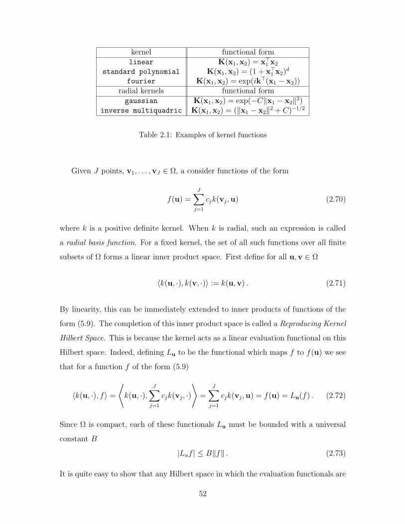
kernel functional formlinear K(x1,x2) = x>1 x2
standard polynomial K(x1,x2) = (1 + x>1 x2)d
fourier K(x1,x2) = exp(ik>(x1 − x2))radial kernels functional formgaussian K(x1,x2) = exp(−C‖x1 − x2‖2)
inverse multiquadric K(x1,x2) = (‖x1 − x2‖2 + C)−1/2
Table 2.1: Examples of kernel functions
Given J points, v1, . . . ,vJ ∈ Ω, a consider functions of the form
f(u) =J∑
j=1
cjk(vj,u) (2.70)
where k is a positive definite kernel. When k is radial, such an expression is called
a radial basis function. For a fixed kernel, the set of all such functions over all finite
subsets of Ω forms a linear inner product space. First define for all u,v ∈ Ω
〈k(u, ·), k(v, ·)〉 := k(u,v) . (2.71)
By linearity, this can be immediately extended to inner products of functions of the
form (5.9). The completion of this inner product space is called a Reproducing Kernel
Hilbert Space. This is because the kernel acts as a linear evaluation functional on this
Hilbert space. Indeed, defining Lu to be the functional which maps f to f(u) we see
that for a function f of the form (5.9)
〈k(u, ·), f〉 =
⟨k(u, ·),
J∑j=1
cjk(vj, ·)
⟩=
J∑j=1
cjk(vj,u) = f(u) = Lu(f) . (2.72)
Since Ω is compact, each of these functionals Lu must be bounded with a universal
constant B
|Luf | ≤ B‖f‖ . (2.73)
It is quite easy to show that any Hilbert space in which the evaluation functionals are
52

bounded, there is a positive definite kernel for which Lu(f) = 〈k(u, ·), f〉 [105]. This
explicit identification of the Hilbert Space structure underlying such kernel models
not only helps make proofs trivial, but also results in simple algorithms for solving
optimizations with functions in the RKHS as design variables.
Reproducing Kernel Hilbert Spaces have many favorable properties that make
their study worthwhile. First, there are a variety of choices of k which make the
RKHS dense in L2 such as the Gaussian kernel
k(u,v) = exp(−κ‖u− v‖2) . (2.74)
Several results exist estimating the average distance to functions in L2 for finite
data sets [77, 69, 19]. Second, when the RKHS norm is used as a regularizer or
complexity measure for function fitting, the estimated function is insensitive to small
changes in the data set such as removing or replacing data points [14]. Finally, it has
been shown that kernel functions provide excellent approximations of least-squares
regression functions even when the underlying probability distribution that generates
the data is unknown [19, 29, 70].
2.3.3 The Kernel Trick and Nonlinear Regression
There is another construction of RKHS directly from the kernel that makes the con-
nection to linear regression explicit. Suppose we lift each data point xi with a high
(infinite) dimensional vector xi := Φ(x) via some prescribed mapping Φ and then
solve the linear regression problem with the lifted data. We can interpret this as cre-
ating a very long list of “features” of each data point and using the features to solve
the linear regression problem.
Let K be a positive definite kernel. By Mercer’s theorem
K(x1,x2) =∞∑i=1
λiφi(x1)φi(x2) (2.75)
and the sum converges absolutely.
53
If we lift x by the rule
x = [√
λ1φ1(x),√
λ2φ2(x), . . . ,√
λkφk(x), . . .] (2.76)
we find that,
〈x1, x2〉 = K(x1,x2) (2.77)
The functions φ(x) are the promised features. These features can be computed by
solving an integral kernel eigenvalue problem, but such computations are not always
tractable. Fortunately, we do not need to compute them for most applications. The
matrix K with entries Kij = K(xi,xj) is called the kernel matrix. Unless confusion
arises, I will abuse notation and use K for the kernel matrix and K(x1,x2) for the
kernel function. K is the lifting of the Gram matrix. By the positivity of the kernel,
we know it is a positive semidefinite matrix.
Consider α =∑
i cixi. We can directly compute the norm of ‖α‖2K := α>α as
‖α‖2K =
∑i,j
cicjx>i xj = c>Kc ≥ 0 (2.78)
If x is another point in RD, then
α>x =∑
i
ciK(xi,x) (2.79)
so we can interpret α as a function on the original space X. The kernel trick to
tackle nonlinearities is to replace any x>1 x2 in a linear problem with K(x1,x2). This
is implicitly lifting the data into an RKHS, and, though it may appear ad hoc, is
perfectly rigorous. In particular, replacing the Gram matrix with the kernel matrix,
the solution to the linear regression problem with the lifted data will be
f(x) =L∑
i=1
ciK(xi,x) (2.80)
where c = (K + λ11)−1y>. In the next chapter we will give a direct proof that this f
54

is optimal using a more general theorem called the Representer theorem.
From a practical perspective, any linear function estimation problem which can
be phrased in terms of inner products can be “kernelized” into a nonlinear version
by replacing all inner products in the problem with kernel evaluations. Thus, the
problems of PCA [87], ICA [4] and graph clustering [89] were generalized to their
nonlinear counterparts. In the next chapter I will present a straightforward framework
for augmenting the power of Tikhonov regularization with constraints on the function
outputs that generalizes all of these methods.
55

56
Chapter 3
Augmenting Regression with
Priors
This chapter lays out the foundation for the remainder of the thesis. At the core is
a a powerful cost function (Equation (3.20)) that augments the standard Tikhonov
regularization with priors on the labels and the functional form. This cost function
can be applied to a vast array of data-driven modeling problems and can be optimized
in a principled way via Lagrangian duality.
Our starting point is a new proof of the so-called “Representer Theorem” that
shows how almost any norm-regularized cost function we can pose on an RKHS can
be transformed into a finite dimensional problem. We will see that this theorem is an
immediate consequence of a simple duality argument on the RKHS. By dualizing over
the remaining variables in the optimization, we are able to solve joint optimizations
over the function that we are fitting, the labels of the data points, and the kernel that
defines the Hilbert space.
When learning a mapping, Tikhonov regularization can only take advantage of
labelled data, but constraints on the labels of the unlabelled data can also allow us
to leverage this unlabelled data. Using Kernel PCA [87] as a motivating example,
Section 3.2 shows that augmenting the Tikhonov regularization problem with con-
straints on the hidden y values can lead to optimization problems where the optimal
function includes terms involving the unlabelled data.
57

Finally, Section 3.3 discusses how to incorporate priors on the functional form of
f into learning algorithms. This will result in the problem of selecting the best kernel
function for a given problem. The duality argument of Section 3.1 further implies
that all of the augmented Tikhonov Regularization problems are convex in the kernel
function. When the problem is solvable with a fixed kernel and when a particular
optimization problem can be solved over the set of possible kernels that the problem
will admit a subgradient algorithm for selecting the optimal function form and the
optimal labels for the unlabelled data. This has many implications in the field of
“Kernel learning.” In particular, whenever the cost function is quadratic or polyhedral
and the set of possible kernels defines an affine subset of the positive semidefinite
cone then the resulting problem can be phrased as a semidefinite program. The final
sections of the chapter discuss several examples of kernel learning. In particular, a
new algorithm for computing the best polynomial kernel is presented.
3.1 Duality and the Representer Theorem
In Chapter 2 we discussed a simple optimization over a Reproducing Kernel Hilbert
Space and showed that even though the problem was searching over an infinite di-
mensional space, it could be solved using least-squares. In this section, let us begin
with a very general cost Tikhonov regularization problem over an RKHS. Again, we
will search for a real valued function f in the RKHS that operates on data x. We
will also be interested in optimization over a vector of labels u. The variable u is
a mnemonic for unlabelled data to be optimized over, and the variable y will be re-
served for labelled data that are fixed in advance. Let V be any cost function on the
outputs of f on the data f(xj) and a vector of labels u.
Consider the norm-regularized optimization
minf,u
V (f(x1), . . . , f(xN),u) + λ‖f‖2K (3.1)
The standard Tikhonov regularized regression problem where all of the labels are
58

given as y can be posed in this form by letting V be given as
V (f(x1), . . . , f(xN),y) =N∑
i=1
(f(xi)− ui)2 + δ(u− y) (3.2)
the delta function removes the variable u from the optimization and replaces it with
the constant vector y. This is equivalent to adjoining the equality constraint u = y
to the optimization (3.1).
The following theorem has many proofs and is at the heart of why the RKHS
framework is useful. Chapter 2 presented a circuitous proof by appealing to linear
regression. Other more direct proofs can be found in a variety of sources including,
for example, [35, 88].
Theorem 3.1.1 [Representer Theorem] If f is an optimal solution to (3.1), then f
can be expressed in the representation
f(x) =N∑
i=1
cik(xi,x) (3.3)
This theorem transforms the search over a possibly infinite dimensional space into
the search for a set of N real numbers. The proof I present here will serve as a prequel
to the use of duality in learning in the remainder of the chapter. The representer
form will be an immediate consequence of the solution method. By adding redundant
constraints to the cost function, I will employ Lagrangian duality to eliminate f
in the RKHS. The resulting Lagrange multipliers will precisely be the coefficients
of the expansion (3.3). The proof rests on the following theorem that is proven in
Appendix B.
Theorem 3.1.2 Let V be a real inner product space and let w1, . . . ,wN ∈ V, a ∈ RN .
Let W be the Gram matrix of the wj.
59

(i) The equality constrained norm minimization problem
minv∈V
〈v,v〉
s.t. 〈v,wi〉 = ai for i = 1, . . . , N
(3.4)
has an associated dual program
maxα−α>Wα + 2α>a (3.5)
which is an unconstrained convex quadratic program. The primal optimal value
is equal to the dual optimal value.
(ii) Suppose the optimal value of the primal-dual pair is finite. Then the set of dual
optimal solutions is given by
D := α ∈ RN : Wα = a (3.6)
and the set of primal optimal solutions is given by
P := N∑
i=1
αiwi : α ∈ D (3.7)
With this theorem in hand, let us proceed to a
Proof [of the Representer Theorem] First, introduce a new variable z ∈ RN and
add the constraints
zi = f(xi) = 〈f, k(xi, ·)〉K (3.8)
to the primal problem for i = 1, . . . N . This results in the optimization
minf,z,u
V (z,u) + λ〈f, f〉K
s.t. zi = 〈f, k(xi, ·)〉K for i = 1, . . . , N
(3.9)
Now we can dualize over the f variable alone. Since the first summation does not
60
depend of f , we can ignore it when optimizing over f and consider the inner-most
minimization
minf
〈f, f〉K
s.t. zi = 〈f, k(xi, ·)〉K for i = 1, . . . , N
(3.10)
This is precisely an equality constrained norm minimization on the RKHS of the
form (3.4). By Theorem 3.1.2, the dual optimization is given by the unconstrained
quadratic program
maxc
2c>z− c>Kc (3.11)
This is an unconstrained quadratic program. The set of dual optimal solutions is
given by the set of solutions to Kc = z. When z is in the range of K, the optimal
cost is given by z>K†z. Plugging this into the original problem gives an optimization
free of both f and c.
minz,u
V (z,u) + λz>K†z
s.t. z ∈ Ran(K)
(3.12)
Given the optimal z∗, we can compute
c∗ = K†z∗
f ∗ =N∑
i=1
c∗i k(xi, ·)(3.13)
There are two useful alternative formulations of the Tikhonov regularization prob-
lem. First we can substitute the value Kc in for z and eliminate the z variable. This
results in the standard representer form that appears in the literature
minc,u
V (Kc,u) + λc>Kc (3.14)
Secondly, to avoid the numerical difficulties involved in the computation of pseu-
61

doinverses, we can employ the Schur complement lemma to yield an equivalent opti-
mization
minz,u,t
V (z,u) + λt
s.t.
t z>
z K
0(3.15)
The equivalence follows immediately from the following simple whose proof can be
found in Appendix A
Lemma 3.1.3 Let A 0 be n× n, x ∈ Rn, and t ∈ R. Then t x>
x A
0 (3.16)
if and only if x is in the range of A and x>A†x ≤ t.
This reformulation shows that the arbitrary learning problem (3.1) can be formulated
such that the kernel matrix appears only in a matrix inequality of the form of (3.15).
This inequality is convex in the matrix K, and since each entry of K is simply an
evaluation of a kernel function, the optimization is convex in the kernel function. In
particular, if the optimization is jointly convex in z and y, then it it is convex in both
the outputs and the kernel function, and can be solved efficiently. In the Section 3.3
we present a general algorithm for solving this problem. We show that in the case that
the cost and K are both semidefinite representable, then the kernel learning problem
can be solved with semidefinite programming.
As an interesting application of the reasoning used in the proof of Theorem 3.1.1,
we can show that unseen or unconstrained data has no effect on the optimal f . Indeed,
consider the norm minimization problem with N + M data points, the first N fixed,
and the last M free:
minf,zN+1,...,zN+M
〈f, f〉K
s.t. zi = 〈f, k(xi, ·)〉K for i = 1, . . . , N + M
(3.17)
62

Once again, consider the dual problem with respect to the variables f , zN+1, . . . , zN+M
by forming the Lagrangian with zi fixed for i = 1, . . . , N .
L(f, zN+1, . . . , zN+M , c) = 〈f, f〉 − 2〈f,N+M∑i=1
cik(xi, ·)〉+N+M∑i=1
cizi (3.18)
Let us first minimize jointly over zi for i = N +1, . . . , N +M . In this case, when any
of the corresponding ci 6= 0 for i = N + 1, . . . , N + M , the Lagrangian is unbounded
below. Therefore, ci must equal zero in the kernel expansion and the unconstrained
data points have no influence on the optimal f . There is again no duality gap, because
at the dual optimal c, the primal optimal f has norm
‖N+M∑i=1
c∗i k(xi, ·)‖2 = c∗>Kc∗ (3.19)
which is the dual optimal value. In the next section, we will demonstrate how to
leverage unlabelled data by constraining the labels of ui at the unlabelled points.
3.2 Augmenting Regression with Priors on the Out-
put
Rather than using a very general cost V , it will be useful to restrict attention to a
more narrow generalization of the least-squares cost of Chapter 2. By a cost function,
I mean a real valued function C : R × R 7→ R such that C ≥ 0 and for every a,
there exists a b(a) such that C(a, b(a)) = 0 and for every b there exists an a(b)
such that C(a(b), b) = 0. Certainly, the least-squares cost satisfies these properties.
In Chapter 4, we will encounter the hinge loss of the support vector machine [101]
which is a also cost function of this form.
Consider the following special case of (3.1)
minf,u
1
N
N∑i=1
C(f(xi), ui) + λ‖f‖2K + S(u) (3.20)
63

where C is any cost function and S is any extended-real valued function on Rn.
Following the same reasoning as in the proof of the Representer Theorem, we must
have that the optimal f has the form of Equation (3.3). This is true for any function
S.
A “prior on output” is just a choice of the function S. The most trivial example
is in the case of the standard regression where for each xi we are given labels ui = yi.
Here
S(y) :=
0 ui = yi ∀i
∞ otherwise
(3.21)
In this case, we can directly minimize over y by plugging these values into the cost
function. Then we can in turn solve for f .
Moving beyond this trivial cost, S, we shall see that a surprising number of well
known algorithms can be cast in the form of Equation (3.20). Furthermore, Chap-
ters 4– 6 will present new novel applications of this seemingly simple framework.
3.2.1 Least-Squares Cost
When the cost is the least-squares cost, we can directly minimize it respect to f and
are then left with an optimization only over the labels u and the kernel matrix K.
Beginning with the optimization
minf,z
L∑i=1
(zi − ui)2 + λ‖f‖2
K
s.t. 〈f, k(xi, ·)〉K = zi
(3.22)
we can construct the joint dual problem over f and z. Again constructing a La-
grangian
L(f, z, c) =N∑
i=1
(zi − ui)2 + λ〈f, f〉K − 2λ〈f,
N∑i=1
cik(xi, ·)〉+ λ
N∑i=1
cizi (3.23)
64
Minimizing over f yields the representer form (3.11). To minimize over z, note that
we can minimize over each zi individually. By differentiating, we find
minz
(z − u)2 + 2λcz = −λ2c2 + 2λcu (3.24)
Plugging this into the Lagrangian gives the dual problem
λ maxc −λc>c + 2u>c− c>Kc (3.25)
This can be readily solved to give the optimal solution
c = (K + λ11)−1u (3.26)
Plugging this back into the dual problem yields the following expression for the cost
of the optimal function f in the regularized least-squares problem
CT (u,K) := λu>(K + λ11)−1u (3.27)
called the Tikhonov cost. Equation (3.27) will be a focus throughout. It is jointly
convex in u and K and no matter what cost S(u) we add to the Tikhonov loss, we
can always solve for f to produce a term of this form for y. That is, when we choose
C to be the least-squares cost, Equation 3.20 can be written as an optimization only
over u
minu
λu>(K + λ11)−1u + S(u) (3.28)
If we want to determine f , we may take the optimal y and let c = (K + λ11)−1y.
Then the optimal f is given by the kernel expansion
f(x) =N∑
i=1
ciK(xi,x) (3.29)
65
3.2.2 The Need for Constraints
In the case that some of the yi labels are withheld, the standard Tikhonov regular-
ization problem cannot make use of any of the unlabelled data points in the kernel
expansion. Indeed, if a label yk is withheld for a data point xk, we can still include
it in the loss function and solve for the optimal label uk. Without loss of generality,
we may assume k = 1.
minf,u1
N∑i=1
C(f(xi), ui) + λ‖f‖2K
s.t. ui = yi i = 2, . . . , N
(3.30)
Since u1 can always be set to force C(f(x1), u1) = 0, the outputs of f are only
constrained at xi for i = 2, . . . , N . As reasoned in Section 3.1, this means that c1 = 0
in the representer form.
For the least-squares cost, we can derive this result directly by plugging in the
representer form for f(x) and showing that ck = 0. First we solve the optimization
λ minu1
u>(K + λ11)−1u (3.31)
for u1. To do so, let y2 denote the vector of labels 2 to N . Partition the kernel matrix
around the first entry as
K =
K11 K12
K21 K22
(3.32)
where K11 is 1 × 1, K12 = K>21 is 1 × (N − 1) and K22 is (N − 1) × (N − 1). Let
Q = (K + λ11)−1 be partitioned in the same way as K
Q =
Q11 Q12
Q21 Q22
(3.33)
66

Then, ignoring the constant multiple λ, we would like to solve
minu1
u21Q11 + 2u1Q12y2 + y>2 Q22y2 (3.34)
since the last term is not a function of u1, we can ignore it. Using the least squares
formula and the form of the inverse of a partitioned matrix found in Appendix A, we
find
u1 = − 1
Q11
Q12y2
= −(K|K22)(−(K|K22)−1K12K
−122 )y2
= K12K−122 y2
(3.35)
Note that if f ∗2 is the minimizer of the optimization trained on x2, . . . ,xL, then
u1 = f ∗2 (x1). Now we can plug this form into the function learned from x1, . . . ,xL
c1 = Q11u1 + Q12y2 = 0 (3.36)
as claimed.
The preceding reasoning shows that one may consider Tikhonov regularization as
an optimization over labelled and unlabelled examples. The functional representation
does not make use of the unlabelled data, but the hidden labels and the representer
form can be optimized simultaneously. On the other hand, if we can yield functional
representations that use the unlabelled data if we constrain the outputs at those data
points away from their automatic solution in Tikhonov regularization. This will be
illustrated in the sequel.
67

3.2.3 Priors on the Output
Let us now present our first example of how constraints allow for representer forms
that exploit the unlabelled data. Consider the cost function
S(u) =
0 1N
∑Ni=1 u2
i = 1
∞ otherwise
(3.37)
This cost enforces the constraint that the set of labels must have empirical variance
1. Consider the situation when there are no labels given at all. If we adjoin the
preceding cost to the Tikhonov cost, we can form the optimization problem
minf,u
N∑i=1
(f(xi)− ui)2 + λ‖f‖2
k
s.t.1
Nu2
i = 1
(3.38)
Using the form for the least squares cost, this reduces to
minu
λu>(K + λ11)−1u
s.t. u>u = N,
(3.39)
This is an eigenvalue problem, the optimal solution of which is the greatest eigenvector
of K scaled so that it has norm√
N . In particular, the optimal u is not 0. This is
because we only allow non-zero solutions by enforcing the variance constraint. Having
computed the optimal u, we can, again solve for the optimal function f . Since u is
nonzero, the kernel expansion will include terms from all of the data even though no
labels were given.
Let us now consider the situation where we are looking for d functions f (i), i =
1, . . . , d, at once. Again, we will provide no labels for the data but will supply a
variance constraint. Let f(x) denote the vector valued function from RD to Rd with
ith component f (i). We will search for a matrix of labels U with Uij denoting the
hidden label for data point xj and component i. Uj will denote the vector of labels
68
for point xj. We can form the cost function
minf ,U
N∑i=1
‖Ui − f(xi)‖2 + λ
d∑i=1
‖f (i)‖2K
s.t.1
NUU> = 11,
(3.40)
where the norm of each dimension of f is penalized individually and the labels are
required to have the identity matrix as their empirical covariance. Substituting in
the representer form for each component of f , we can define a matrix of weights C
such that
f (i)(x) =N∑
i=1
Cijk(xi,x) (3.41)
The optimization (3.40) can then be rewritten as:
minC,U
‖U−CK‖2F + λ TrCKC> (3.42)
s.t.1
NUU> = 11, (3.43)
where ‖ · ‖F is the Frobenius norm, K is the kernel matrix of the xj.
Rewriting (3.42) as
minC,U
d∑i=1
Ui
Ci
> 11 −K
−K K2 + λK
Ui
Ci
(3.44)
s.t.1
NUU> = 11, (3.45)
where Ci is the transpose of the ith row of C and Ui is the transpose of the ith row
of X, we may minimize over C to find
C∗i = (K + λ11)−1Ui (3.46)
plugging this optimal value back into the cost function yields a minimization only
69

over U
minU
d∑i=1
U>i (K + λ11)−1Ui (3.47)
s.t.1
NUU> = 11, (3.48)
Now the optimal U∗i are the d largest eigenvalues of the kernel K. Let γ1, . . . , γd
be the largest eigenvalues of K and v1, . . . ,vd be the corresponding orthonormal set
eigenvectors. It follows that the optimal C∗i are given by
C∗i =
√N
γi + λvi (3.49)
Substituting this C∗i into the representer form gives us a solution for f∗
f (i)(x) =
√N
γi + λ
N∑j=1
vijK(xj,x) (3.50)
To summarize, finding the optimal U∗ reduces to extracting the d largest eigenvectors
of the kernel matrix K. The rows of the optimal C∗ are scaled versions of the rows
of U∗.
This first example of regression with an output prior provides a function learning
interpretation of the kernel principal components algorithm (KPCA) of Scholkopf et
al.[87]. KPCA uses the kernel trick of Chapter 2 to “kernelize” the standard principal
component analysis problem from pattern recognition. Instead of operating on the
data points xj, they perform KPCA of the covariance matrix of the lifted data xj in
a Reproducing Kernel Hilbert Space. KPCA returns the functions h1, . . . , hd given
by
hi(x) =1√
γi
N∑j=1
vijk(xj,x) (3.51)
70

from which we see that the f ∗i are multiples of the solution to the kpca problem
f ∗i =
√γi
(γi + λ)2hi . (3.52)
This interpretation reveals that KPCA looks for a smooth function f that projects
the sequence of observations X to a low-dimensional sequence U so that the dimen-
sions of U are orthogonal to each other and have unit sample variance. By placing
an additional prior on the hidden sequence U, we can refine this algorithm to take in
to account a wide range of priors. In particular, in Chapter 5 we can constrain the
U to have linear Gaussian dynamics and in Chapter 6 we will search for unit norm
functions that are zero on all of the given examples.
3.2.4 Semi-supervised and Unsupervised Learning
A semi-supervised, or transductive, learning problem is one where we are given N
data points x1, . . . ,xN with labels for those i that are in a subset S ⊂ 1, . . . , N.
For our purposes, all semi-supervised algorithms are of the form
minf,u
1
N
N∑i=1
C(f(xi), ui) + λ‖f‖2K + S(u)
s.t. ui = yi for i ∈ S
(3.53)
with S a given extended real-valued function.
Unsupervised learning problems are those where we are given N data points
x1, . . . ,xN and no labels at all. For example, the optimization that re-derives ker-
nel PCA is an unsupervised learning problem. In this case, we must guarantee that
minu S(u) ≤ S(0) or else the optimal function and labels will both be identically zero.
In all of our applications, we will set S(0) = ∞ to avoid this trivial solution. In the
KPCA case, we forced the variance of the output to be the identity matrix, and so
the all-zero solution was not feasible.
71

3.3 Augmenting Regression with Priors on Func-
tional Form
Suppose that we know f is an element of a Reproducing Kernel Hilbert Space, but
we do not know the best form for the kernel function. For example, in the case of a
Gaussian kernel,
k(x1,x2) = exp(−C‖x1 − x2‖2) (3.54)
modification of the parameter C greatly changes the character of the function space.
When C is very small, k is nearly the constant function, and when C is large, k(x, ·)
approaches a delta function at x. What is the best way to set this parameter C?
The problem of selecting the kernel best suited to a fitting problem from a family
of kernels is called “kernel learning.” Kernel learning consists of two components:
selecting the best parametrization of a family of kernels and choosing the best cost
functional over these parameters. One of the most popular methods used in the
machine learning community is minimizing the leave-one-out error [17]. It turns out
that even the simple problem of selecting the best parameter C for a Gaussian kernel
by minimizing the leave-one-out error is not convex and can be quite computationally
intensive even find a local minimum.
Kernel Learning has received a good deal of attention of late. Simple local search
methods to directly minimize the Tikhonov cost have been proposed [17], but such
minimizations are often not convex and may result in undesirable local minima.
Lanckriet et al [56] have shown how to apply semidefinite programming to choose
the best convex combination of a finite set of kernels for support vector machines.
But if one was searching over more than one parameter, such convex combinations
cannot efficiently grid the entire space of kernels. Even for searching for the best
convex combination of Gaussian kernels, it has been shown that one kernel for each
data point is necessary to achieve optimality [1].
Our approach in this section is to directly minimize the Tikhonov regularization
problem augmented with a prior on the output to select the best outputs y and best
72
kernel K in a set K simaltaneosuly. We have already seen that the arbitrary Tikhonov
regularization problem (3.1) is convex in the kernel matrix K and hence in the kernel
function itself. We will show furthermore that as long as we can solve the problem
maxK∈K
v>Kv (3.55)
for all v ∈ RN , then we can solve the dual of the kernel learning problem. In
particular, if K is a convex set, then the resulting primal optimization is convex.
When the cost function can be solved by semidefinite program for a fixed K and if
K can be defined as a projection of the semi-definite cone, then the kernel selection
problem can be solved by semidefinite programming. We will end the discussion with
three examples of different families of kernels and the computational considerations
for each.
3.3.1 The Dual of the Arbitrary Regularization Problem
Whereas in Section 3.1 we derived the representer theorem by dualizing over the
RKHS decision variable in the general Tikhonov Regularization problem (3.1), we
could have derived a joint dual program over all of the decision variables z, u and
f . In this case we would need to minimize the Lagrangian with respect to all of the
variables at once. Furthermore, we can be even more ambitious and dualize over the
reproducing kernel itself! Our approach in this section is to directly minimize the
general Tikhonov regularization problem (3.1) to select the best outputs u and best
kernel K in a set K simultaneously. In particular, we have already seen that if K is a
convex set, then the resulting primal optimization is convex in K. In this regard, all
of the problems addressed in this work are convex the kernel matrix K and hence in
the kernel function itself.
Beginning with the optimization (3.9), construct the Lagrangian over all of the
variables
L(f, z,u, k, c) = V (z,u) + λ〈f, f〉K + 2λN∑
i=1
ci(zi − 〈f, k(xi, ·)〉K) (3.56)
73

and minimize over each variable in turn. First, we have seen that for fixed z, u, and
k, we can minimize over f to yield
V (z,u) + 2λc>z− λc>Kc (3.57)
The remaining optimization is now directly a function of the kernel matrix K. The
function
V ∗(c,d) := maxz,u
c>z + d>u− V (z,u) (3.58)
is called the conjugate dual of V [12]. It is easy to check that this function is convex.
Minimizing with respect to f ,z, and u gives the dual problem
maxc−V ∗(−2λc, 0)− λ max
K∈Kc>Kc (3.59)
There are many consequences of this derivation. First, whereas the primal was a
joint optimization over infinite dimensional Hilbert spaces and the functions therein,
the dual problem is always an optimization over RN where N is the number of data
points. In the following section, I will describe a simple subgradient algorithm for
optimizing (3.59) when we can efficiently extract the maximizing K for each c and
can compute V ∗.
If V is a strictly convex function and the set K is convex and has a point in the
relative interior, then the optimal value of this optimization is equal to the optimal
value of the primal optimization. That is, there is no duality gap. In particular, we
can extract the optimal kernel by finding the maximizer
K∗ = arg maxK∈K
c∗>Kc∗ (3.60)
The specifics of the set K completely determine the complexity of this kernel
learning. For example, if K can be represented as a set of linear matrix inequalities
and V is quadratic or piecewise linear, then (3.59) is a semidefinite program. This
generalizes all of the algorithms presented in [56] to generic cost functions with ar-
74

bitrary priors on the the u values. In the case that K is not convex, then the dual
of the dual program can be interpreted as searching over the convex hull of K. The
final sections highlight some special cases of K.
3.3.2 A Decomposition Algorithm for Solving the Dual Prob-
lem and Kernel Learning
We consider a simple subgradient algorithm for solving (3.59) under the assumption
that we can solve the problem
maxK∈K
v>Kv (3.61)
and can compute the function V ∗(v) for all v ∈ Rn.
Define the functions
q(c) := V ∗(2λc, 0) + m(c)
m(c) := maxK∈K
c>Kc(3.62)
and let D denote the domain of V ∗. We seek to minimize q. First, we compute
subgradients. Note that
∂q(c) = 2λ∂V ∗(2λc, 0) + ∂m(c)
∂V ∗(c) = z∗ ∈ RN : c>z∗ − V (z,u) = maxz,u
c>z− V (z,u)
∂m(c) = K∗c : K∗ ∈ K and c>K∗c = maxK∈K
c>Kc
(3.63)
which yields the following subgradient algorithm. Choose a sequence of step sizes tk
with∑∞
k=1 tk = ∞ and tk → 0.
(i) Begin with a random c ∈ D
(ii) Set s = z∗+K∗c where z∗ ∈ arg maxz,u 2λc>z−V (z,u) and K∗ ∈ arg maxK∈K c>Kc.
(iii) Let c = (c− tks)+ where (·)+ denotes the orthogonal projection onto D
(iv) Let k = k + 1 and repeat.
75

This algorithm will compute an optimal solution, c∗ to the convex program (3.59).
Furthermore, when V is strictly convex the outputs of the optimal function f are given
by
f ∗(xi) = zi
z∗ = arg maxz
2λc>z− V (z,u)(3.64)
and if K is a convex set with a point in its relative interior, then an optimal kernel is a
maximizer of K∗ ∈ arg maxK∈K c>Kc. The analysis of convergence of this algorithm
can be found in a variety of places including [7, 11, 12].
3.3.3 Example 1: Finite Set of Kernels
Let us consider the simple case where K is the finite set of kernels K1, . . . ,KM.
The dual problem is
−minc
(V ∗(c) + max1≤i≤M
c>Kic) (3.65)
or
−minc,γ
(V ∗(c) + γ)
s.t. c>Kic ≤ γ
(3.66)
the associated dual of this problem amounts to learning the best convex combination
of the M kernels
minz,t,p
V (z,y) + λt
s.t.
t z>
z∑M
i=1 piKi
0
p ≥ 0,M∑i=1
pi = 1
(3.67)
In particular, this semidefinite program generalizes the algorithm in [56] where the
cost function was assumed to be a support vector machine loss. This problem takes
76

on an interesting form when the cost is the least-squares cost
minf,K
L∑i=1
(f(xi)− yi)2 + λ‖f‖2 (3.68)
As we have noted before, applying the Representer Theorem and solving for f gives
the Tikhonov cost
CT (K) := λy>(K + λ11)−1y (3.69)
This is convex in K. Indeed if we parameterize K as
K =T∑
i=1
αiKi (3.70)
then by the Schur Complement Lemma
minα
λy>(K + λ11)−1y = mint,α
λt
s.t.
t y>
y∑T
i=1 αiKi + λ11
0(3.71)
which is a semidefinite program.
We may apply any set of linear constraints to the αi and preserve convexity.
In particular, if αi are on the T -simplex then we are searching for the best convex
combination of a given set of kernels.
mint,α λt
s.t.
t y>
y∑T
i=1 αiKi + λ11
0
αi ≥ 0∑T
i=1 αi = 1
(3.72)
Since C(z) = (y− z)2, then we have seen in Section 3.2.1 that C ∗ (c) = 14c2 + cy.
77

The dual program for this problem is thus given by
maxc,γ −c>c + 2y>c− γ
s.t. c>Kic ≥ λγ(3.73)
This is quite similar to Lanckriet’s Kernel selection program for the SVM [56]. In
particular, this can be solved using a second-order cone programming solver [61] which
is generally more efficient than solving a semidefinite program.
3.3.4 Example 2: Gaussian Kernels
Let K be the set of all Gaussian kernels
K = K(x,y) = exp(−θ‖x− y‖2) : θ > 0 (3.74)
For a fixed data set, let K[θ] denote the kernel matrix generated from the Gaussian
kernel with parameter θ. In this case the dual of the kernel selection problem is the
semi-infinite program
−minc,γ
(V ∗(c) + γ)
s.t. c>K[θ]c ≤ γ ∀θ ≥ 0
(3.75)
This problem is convex and strictly feasible as if we let γ ≥ supθ c>K[θ]c, we can
satisfy the all of the inequalities strictly.
The dual of this dual problem amounts to selecting the best kernel from the convex
hull of the Gaussian kernels. Using the dual, we can provide an elementary proof that
the optimal selection for convex combination of Gaussian kernels for a data set with
N points is given by a convex combination of N kernels. This result was derived in [1]
by a lengthy argument assuming a differentiable cost V .
However, for an arbitrary convex cost, the expansion is an immediate result of
classic results from semi-infinite optimization (see, for example, [36, 44, 62] for a
proof).
78

Theorem 3.3.1 Given a semi-infinite optimization
minx
f(x)
s.t. g(x,y) ≤ 0, ,y ∈ Ω
(3.76)
with x ∈ Rn, Ω ⊂ Rm compact, f convex, suppose there exists a x such that g(x,y) <
0 for all y ∈ Ω. Then x∗ is a global minimizer of (3.76) if and only if there exist
µ1, . . . , µn ≥ 0, y1, . . . ,yn ∈ Ω such that
∇f(x∗) +n∑
i=1
µi∇g(x∗,yi) = 0 (3.77)
The proof of this theorem is a mild generalization of the classical Slater condition
to the semi-infinite case. One shows that 0 is in the convex hull of ∇f(x∗) ∪
∇g(x∗,y) : y ∈ Ω and that the coefficient of ∇f(x∗) can always be chosen to be
non-zero. Then, by Caratheodory’s theorem, such a convex combination can be found
using only n vectors.
As an immediate consequence, we have
Corollary 3.3.2 For any convex cost V , the optimal kernel for (3.86) with K as in
(3.74), the optimal K is given by
K∗ =N∑
i=1
piK[θi] (3.78)
for some nonnegative pi,θi with∑
i pi = 1
Proof The optimization (3.75) is strictly feasible. By Theorem 3.3.1, a necessary
and sufficient condition for optimality of is the existence of pi,θi with∑
i pi = 1 such
that
z∗ + (N∑
i=1
piK[θi])c∗ = 0 (3.79)
and that there is no duality gap. Thus, the optimal kernel has the desired form.
Equation (3.79) is nothing more than the KKT conditions for the dual problem.
79

From a practical perspective, this result is discouraging. It seems excessive to
have one kernel for every data point in the training set. This is especially true in
the case of the Gaussian kernels where there is only one parameter to optimize. For
smooth cost functions V , the cost function (3.86)is Lipshitz continuous in the single
parameter C, and, arguably, a simple search like Brent’s 1-d optimization algorithm
would find the optimal solution by solving the Tikhonov regularization problem for
a few choices of C.
Furthermore, even when content to search for a large convex combination of ker-
nels, the optimal centers θi can be difficult to find. Argyriou et al [1] propose a
greedy algorithm that is not even guaranteed to converge after n steps. Indeed, it
may converge arbitrarily slowly. For these reasons, it is interesting to consider the
case of polynomials where the search is convex in the kernel parameters.
3.3.5 Example 3: Polynomial Kernels
Polynomials are attractive for kernel learning as the positivity of polynomial kernels
is easy to characterize and they can be parametrized as a subset of the semidefinite
cone. In this section, we will first characterize the set of polynomial functions that
are positive definite. Then we will describe semidefinite program for selecting the
optimal polynomial kernel.
Let x ∈ Rd and denote the vector of monomials of degree less than or equal to p
by xp.
Theorem 3.3.3 Let k(x,y) be a symmetric polynomial of degree 2p on a compact
set of infinite cardinality Ω ⊂ Rd. Then k(x,y) is a positive definite kernel on Ω if
and only if
k(x,y) = x>p Qyp (3.80)
for some positive semidefinite matrix Q.
There are several properties of this theorem that are worth remarking upon. First,
for those familiar with positive polynomials, note that there is no ambiguity in the
80
definition of the matrix Q unlike in the case of polynomials where Q is only defined
as an affine subspace. Second, in the kernel learning optimization (3.86), the matrix
Q appears linearly in the constraint and we can directly minimize with respect to
this variable. Any prior information about the terms to include in Q or relations
amongst the components of Q can be immediately included in the optimization. We
now present a simple proof for the theorem.
Proof [of Theorem 3.3.3]
Sufficiency of Equation (3.80) can be seen by picking x1, . . . ,xN ∈ Ω and c1, . . . , cN ∈
R. Let X = [x1, . . . ,xN ] and c = [c1, . . . , cN ]>. Then since Q 0 we have
N∑i,j=1
cicjk(xi,xj) = c>X>QXc ≥ 0 (3.81)
proving that k is a positive definite kernel.
To prove the converse, first note that by Mercer’s Theorem,
k(x,y) =∞∑i=1
λiΦi(x)Φi(y) (3.82)
where ∫Ω
k(x,y)Φi(y)dy = λiΦi(x) (3.83)
and λi ≥ 0. The theorem will be proven if we can show that the series (3.82) is finite
and that all of the eigenfunctions are polynomials. In this case, we can construct the
positive semidefinite matrix Q in Equation (3.80) by letting qi be the vector such
that Φi(x) = q>i xp. Plugging this into the Mercer expansion gives
k(x,y) =I∑
i=1
λix>qiq
>i y (3.84)
Let Q :=∑I
i=1 λiqiq>i . It is a positive combination of outer products and hence must
be positive semidefinite as desired.
To prove that the Mercer expansion is a finite sum of polynomials, consider the
81

functions indexed by y ∈ Ω
fy(x) := k(y,x) (3.85)
Finite sums∑N
j=1 αjfyjare polynomials of degree at most p. Hence, the span of the
fy lies in the finite dimensional subspace of L2(Ω) consisting of polynomials of degree
less that or equal to p. Since all finite dimensional subspaces of L2(Ω) are closed,
all of the limit points of the set of fy must be polynomials of degree less that or
equal to p. In particular, the integral on the left hand side of (3.83) is a limit point
of the fy and must be a polynomial. Consequently all of the Φi are polynomials of
degree at most p. It remains to prove that there are only a finite number of Φi in
the expansion. But this follows because Φi are an orthonormal sequence in a finite
dimensional subspace of L2(Ω), completing the proof.
Algorithmically, we can take advantage of this theorem as follows. First, let
X = [x1, . . . ,xN ] denote the data matrix and X = [x1, . . . , xN ] denote the matrix of
data lifted to a list of monomials of degree less than or equl to p. The kernel learning
optimization for polynomial kernels is given by
minz,t,Q
V (z,y) + λt
s.t.
t z>
z X>QX
0
Q 0
(3.86)
By making Q sufficiently large, this cost of this optimization can be made arbitrarily
small. Thus, we must constrain the maximal value for Q. This can be done in a
variety of ways, but the easiest constraint to adjoin is Tr(Q) ≤ β for some β > 0.
This can be also adjoined to the cost as a penalty function when the value β is not
known explicitly. On the other hand, there is no reason not to just have β = 1 as
this simply sets a scale for the polynomial feature space.
82
3.4 Conclusion
In this chapter, I have shown that an arbitrary Tihkonov cost function can be aug-
mented with priors on hidden labels, and then jointly optimized over the functions,
kernels, and labels. Using tools from Lagrangian duality, I have shown that these
optimizations are tractable, and recover a variety of learning algorithms.
The remainder of this document will focus on particular instances of the cost
function S(y). In Chapter 4, I will require that yi = ±1. This problem, though NP-
HARD, will generalize the standard kernel methods for clustering and transduction.
In Chapter 5, I will require that y lie near the outputs of a linear dynamical system.
This will serve as a powerful method for transforming time series with very few
examples and dimensionality reduction. Finally, in Chapter 6, I will require that y
be a constant vector. This will result in a method for learning manifolds of low-
codimension with applications in anomaly detection. As we have seen, all of these
algorithms are also convex in the kernel function, so if prior information on functional
form is provided, then it can be incorporated into these learning algorithms as well.
83

84
Chapter 4
Output Prior: Binary Labels
One of the most successful applications of Tikhonov regularization on Reproducing
Kernel Hilbert Spaces has been data driven classifiers. Classifiers return discrete class
labels as output. For instance, a classifier could take as input an image and return
whether the image was of a cat or a dog, or it might take a piece of music and return
whether it was written by Mozart or Beethoven. A common approach to training
such classifiers is to provide labels y = ±1 for each x in the training set. If a training
example is in the first class it is assigned a 1. If it is in the second class, it is assigned
a −1.
The classification algorithms differ in their choice of cost function. Most famous
is Vapnik’s Support Vector Machine [13, 101] where the cost function is the so-called
hinge loss
V (f(x), y) = max(0, 1− f(x)y) . (4.1)
This cost function assigns no penalty if f(x) is of the same sign as y and is of
greater magnitude than 1 and assigns a linearly increasing penalty otherwise. Another
method, regularized least-squares classification, just uses the least-squares cost. Even
though it might not make intuitive sense to use a least squares cost for classification,
the RLSC algorithm, when well tuned, performs as well as the SVM and has certain
computational advantages [84, 83].
In this chapter we will look at the situation where some of the class labels are
85

withheld. In the absence of the labels, we will constrain the output values to be either
+1 or −1. This constraint is non-convex, and as we will see, finding the optimal
labels is NP-HARD. However, we will show that we can approximate the optimal
labels with a variety of algorithms. Using Lagrangian duality, we will develop a
class of semidefinite programming problems that approximate the semi-supervised
classification and segmentation problems arising from Tikhonov regularization with
quadratic or polyhedral cost functions.
The semidefinite programs we derive can be solved quickly for sets of a few hun-
dred examples. For problems where there are thousands of variables, however, the
semidefinite programming problems may not even fit in memory. To fix this prob-
lem, we discuss a class of eigenvalue approximations derived from these semidefinite
programs. These approximations include the well-known spectral clustering algo-
rithms [103]. In particular, this derivation reveals the functions that the spectral
clustering algorithms are implicitly learning.
The semi-supervised classification problem is often called transduction. Several
algorithms have been proposed to solve the transductive problem introduced in [100].
Joachims provides a local search method for the transductive SVM which is fast but
subject to local minima [49]. Similarly, Smola et al present a local-search method for
solving the transductive problem for the least-squares cost [94]. In [25], the authors
construct a relaxation of the standard support vector machine problem by relaxing the
rank one product outer product of the labels vector. Unfortunately, since they relax
the dual form of the SVM rather than the primal Tikhonov regularization problem, the
resulting semidefinite program cannot be solved for more than one hundred variables.
The relaxation we present can be solved for a several thousand variables by solving
the associated dual.
In the case when no labels are given at all, we are searching for a function which
divides a data set into two classes. This unsupervised learning can be interpreted
as segmentation or clustering, where, instead of fitting a mixture model to tessellate
the data, we search for a smooth function whose zero set passes through the data
separating it into two sets.
86

The Normalized Cuts clustering algorithm of Shi and Malik, although originally
presented as spectral relaxation of a graph-cut problem, can be interpreted as a
relaxation of the unsupervised Tikhonov regularization problem. Normalized Cuts
views the data set as a graph, where nodes represent data points and edges are
weighted according to the similarity, or “affinity”, between data points. This is the
starting point of many other graph-based clustering algorithms [103, 2]. The affinity
matrix used in these algorithms is a kernel matrix derived from some positive definite
function and hence is a Gram matrix on some RKHS. We show that Normalized Cuts
may be interpreted as learning a function in this RKHS that labels points by the sign
of this function.
This new interpretation of Normalized Cuts reveals that it weights data points
away from the mean of the data set more than those in the center of the data set.
This weighting causes Normalized Cuts to sometimes break elongated clusters and to
be sensitive to outliers. By defining a eigenvalue relaxation that gives equal weight
to all data points, we derive a clustering algorithm (the Average Gap algorithm)
that does not exhibit these problems. Finding labels under this new gap reduces to
thresholding the top eigenvector of a matrix.
This chapter only presents 2-way clustering algorithms. If more clusters are
sought, each 2-way cut can be further subdivided by running the clustering procedure
recursively [90].
4.1 Transduction, Clustering, and Segmentation
via constrained outputs
Since most classification algorithms are trained with y labels set to either +1 or −1,
an intuitive solution to utilize the unlabelled data is to constrain the unlabelled data
to be either plus one or minus one. Let L = N + M with the points x1, . . . ,xN
labelled the points xN+1, . . . ,xN+M unlabelled. The optimization we shall study for
the remainder of the chapter is
87

Problem 1 RKHS Transduction Find a set of assignments to optimize
minf,uM
L∑i=1
C(f(xi), ui) + λ‖f‖2K
s.t. ui = yi i = 1, . . . , N
ui ∈ −1, 1 i = N + 1, . . . , N + M
(4.2)
The resulting algorithm depends only on the choice of the cost function C and how to
best constrain ui to be binary. This optimization seeks to minimize a convex function
over the non-convex set u ∈ RM : ui = ±1. We will see in the next section that even
for the least squares cost, this problem is NP-HARD for a generic RKHS.
There are several different cost functions one could consider. The first is the
least-squares cost
Problem 2 Transductive Regularized Least Squares Find a minimizer for (4.2)
when C(f(x), y)) = (f(x)− y)2
As previously derived, we may plug in C(f(x), y) = (f(x)− y)2 and solve for the
optimal f to yield the optimization over the unlabelled points
minuM
λ
yN
uM
> (K + λ11)−1
yN
uM
ui ∈ −1, 1 i = N + 1, . . . , N + M
(4.3)
There are two different costs which we will consider, inspired by the support vector
machine. The first is the hinge loss. The second is a hard margin loss that does not
allow for yif(x) to be less than 1.
Problem 3 Transductive Support Vector Machine Find a minimizer for (4.2)
when C(f(x), y)) = max(0, 1− f(x)y)
Problem 4 Hard Margin Transductive Support Vector Machine Find a min-
imizer for (4.2) when C(f(x), y)) = δ+(1− f(x)y)
88

For both notational simplicity and the clarity of presentation, we will formulate
the SVM transduction problems using the form of (3.15) in Chapter 3:
minz,t
V ((zi, yi)) + λt
s.t.
t z>
z K
0(4.4)
Let the matrix A span the null-space of the kernel K. Then, by applying the Schur
complement lemma and Lemma A.7.2 from Chapter 3 we can rewrite (4.4) as
minz
V ((zi, yi)) + λz>K†z
s.t. Az = 0
(4.5)
Let us apply this to Problems 3 and 4. First, the transduction problem with the
standard form of the SVM with a hinge loss is given by
minz,uM
N+M∑i=1
ξi + λzK†z
s.t. uizi ≥ 1− ξi
ui = yi i = 1, . . . , N
ui ∈ −1, 1 i = N + 1, . . . , N + M
ξi ≥ 0
Az = 0
(4.6)
Second, the using the hard margin, we get the problem
minz,uM
λzK†z
s.t. uizi ≥ 1
ui = yi i = 1, . . . , N
ui ∈ −1, 1 i = N + 1, . . . , N + M
Az = 0
(4.7)
89

In this case, the regularization parameter λ is only acting to scale the cost function,
and does not directly effect the optimal z or uM . We will omit this parameter in the
further references to the this problem. We will show in the next section that all three
cost functions are NP-HARD.
Before proceeding, let us remark that in the case that no labelled examples are
available, we need to ensure that the trivial labelling f(xi) = 1 is not in the RKHS.
When there are no labels, we will adjoin the constraint∑N
i=1 f(xi) = 0 to the opti-
mization to avoid this redundancy.
4.2 RKHS Clustering is NP-HARD
We will first show that the clustering problem with least squares cost and no labels,
is NP-HARD. Then we will show that providing an incomplete set of labels the
semisupervised problem is also NP-HARD. Finally, we will show that the variants
related to the SVM are also NP-HARD.
While the following arguments should the reader that is unreasonable to expect
to solve these segmentation problems exactly, this section should not be discourag-
ing! Even the well-known problem of K-Means clustering is NP-HARD, yet heuristic
coordinate ascent algorithms have proven successful for many applications. The re-
mainder of the chapter will apply the approximation techniques from Chapter 2 to
yield powerful algorithms that, in practice, perform quite well.
Our proofs of hardness will be through reductions from the Number Partitioning
Problem, one of the fundamental NP-Complete problems [32].
Problem 5 The number partitioning problem (NPP): Given a set of integers
A = a1, . . . , aN, does there exist a partition of A into two subsets U and V such
that the respective subset sums are equal?
This problem is NP-complete even under particular restrictions. For example, if
one requires that ||U | − |V || ≤ 1, the problem is NP-HARD. Similarly, if, for a fixed
constant c, we are given the assignments for the first cN elements, the problem is
NP-HARD.
90

Problem 6 The “semi-supervised” number partitioning problem (SNPP):
Given a set of integers A = a1, . . . , aL, two integers l and k such that k + l < cL,
does there exist a partition of A into two subsets U and V such a1, . . . , ak ∈ U ,
ak+1, . . . , ak+l ∈ V such that that the respective sums are equal?
This problem is equivalent to the Problem 5. To see this define a new set
B = k∑
i=1
ai −l∑
j=k+1
aj, al+1, al+2, . . . , L (4.8)
If the answer to Problem 6 is YES, then let U and V be the partitions of the set
A. Define U ′ to be the set of all elements aj ∈ U with j > k + l. Define V ′ to be
the set of all elements aj ∈ V with j > k + 1. Then U ′ ∪ ∑k
i=1 ai −∑l
j=k+1 aj
and V ′ are partitions of B with equal subset sums. Similarly, if there is a partition
of B into two sets with equal subset sums, we can construct a partition for A. As a
result of this discussion, we will show in what follows that the unsupervised learning
problem is generically hard, and, as an immediate corollary we will deduce that the
semi-supervised problem is also NP-HARD.
The following lemma identifies NPP with a particular quadratic optimization. We
will reduce the optimization to this form by picking a particular set of input data.
Lemma 4.2.1 The number partitioning problem is equivalent to finding a minimizer
of the binary quadratic program
minu
u>aa>u
s.t. u2i = 1
(4.9)
Proof Let U and V partition A. Let ui = +1 if ai ∈ U and ui = −1 if ai ∈ V .
Then the difference between the subset-sums of U and V is
∑aj∈U
aj −∑ak∈V
ak =L∑
i=1
uiai (4.10)
Therefore, A can be partitioned into a pair of sets with equal sums if and only if there
91

exists a y such that∑L
i=1 uiai = 0. Since
u>aa>u = (L∑
i=1
uiai)2 ≥ 0 , (4.11)
then A has a partition if and only if the minimum of (4.9) is zero.
The following theorem is an immediate consequence of the preceding discussion.
Theorem 4.2.2 Problem 2 is NP-HARD.
Proof Given an instance of NPP, we will reduce it to a clustering problem as
follows. Let a = [a1, . . . , an]> be the column vector containing the elements of the set
a. For i = 2, . . . , N , Let a/||a||,v2, . . . ,vN be an orthonormal basis for Rn. Let
K =[
v2 . . . vN
] [v2 . . . vN
]>(4.12)
Finally, let λ be any positive rational number. It is easy to check that
(1
λK + 11)−1 =
1
(1 + λ)||a||2aa> +
λ
1 + λ11 (4.13)
and hence
arg minu2
i =1u>(
1
λK + 11)−1u = arg min
u2i =1
u>aa>u (4.14)
therefore, if one can find the optimal cluster assignments, one can find the optimal
partitioning of A. It is clear that the analysis remains the same if some of the yi
labels are given or if we require the two clusters to be balanced. This completes the
proof.
Since Problem 2 is a subproblem of Problem 1, we have the following
Corollary 4.2.3 Problem 1 is NP-HARD.
To proceed to the proofs that transduction with the Support Vector Machine
costs is NP-HARD, we introduce a variant of the quadratic program for least-squares
clustering with inequality constraints
92
Problem 7 Given a positive definite N × N matrix Q, find a minimizer of the op-
timization
minu
u>Qu
s.t u2i ≥ 1
(4.15)
Theorem 4.2.4 Problem 7 is NP-HARD
Proof We will show how this problem can be used to solve the NPP problem. Let
a be an integer vector. There exists a partition of this vector into two subsets with
equal sums if we can find a binary u such that u>aa>u < 1.
Let Qβ = aa> + β11. Let
uβ = arg minu2
i≥1u>Qβu (4.16)
then for all q with qi ∈ +1,−1,
u>β aa>uβ + β‖uβ‖2 ≤ q>aa>q + β‖q‖2 (4.17)
Since q2i = 1 for all i, ‖q‖2 = N , so we have
β(‖uβ‖2−N) ≤ q>aa>q−u>β aa>uβ ≤ q>aa>q ≤ maxzi∈−1,+1
q>aa>q = ‖a‖1 (4.18)
Since the left-hand side is bounded for all β, we have
limβ→∞
‖uβ‖2 = N (4.19)
Furthermore, it is easy to check that for u with all entries of magnitude greater than
or equal to 1, the closest vector of norm N is v = sign(u).
Since the function u>aa>u is continuous, there exists a δ such that if ‖ sign(uβ)−
uβ‖ < δ, then
| sign(uβ)>aa> sign(uβ)− u>β aa>uβ| <1
2(4.20)
93

if we choose β large enough, then ‖ sign(uβ) − uβ‖ < δ and hence we can solve the
problem NPP.
Now, as corollaries, we can show
Theorem 4.2.5 Problem 4 is NP-HARD.
Proof Let u = Kc. Then we can rewrite Problem 4 as
minu
u>K†u
s.t. ui ≥ 1
1>u = 0
Au = 0
(4.21)
of which Problem 7 is a special case.
Theorem 4.2.6 Problem 3 is NP-HARD.
Proof By making the regularization parameter small, we can approximate the
solution to Problem 4. In particular, this would lead to being able solve NPP.
4.3 Semidefinite Approximation using Lagrangian
Duality
As noted in the previous section and in Chapter 2, we may identify the constraint
ui ∈ −1, 1 with the quadratic identity u2i = 1. By using this constraint, we may
consider all subproblems of Problem 1 with quadratic or polyhedral costs V as Non-
convex Quadratically Constrained Quadratic Programs (NCQCQP). This set of op-
timization problems are, as discussed in Chapter 2, NP-HARD, but admit powerful
approximation algorithms via their associated Lagrangian dual problem.
Here we present the primal-dual pair of semidefinite programs associated with
the RLS cost. We will use this cost function and the random hyperplane algorithm
presented in Chapter 2 to produce feasible labels assignments for the unlabelled data.
94
Given N+M data points x1, . . . ,xN+M and labels for the first N points, y1, . . . , yN ,
we want to infer cluster assignments for the remaining M points. Let us group as
vectors yN the labels of the first N data points and uM the (unknown) labels of the
last M data points. Also, let us partition the Kernel matrix of the data as
K =
KNN KNM
KMN KMM
(4.22)
Let Q = (K + λ11)−1 and partition this matrix like K to give the optimization
minuM
yN
uM
> QNN QNM
QMN QMM
yN
uM
s.t. u2
i = 1 for i = N + 1, . . . , N + M
(4.23)
This may be further simplified by lumping together the labelled data points. Let
yp := QMNyN and let T := y>NQNNyN . Then the optimization simplifies to
minz,uM
z
uM
> T y>p
yp QMM
z
uM
s.t. u2
i = 1 for i = N + 1, . . . , N + M
z2 = 1
(4.24)
This problem has the same form as the combinatorial optimization problems stud-
ied in Chapter 2. However, rather than maximizing a positive definite form on
−1, 1n, we are minimizing a positive definite form on the non-convex set −1, 1n
and we cannot produce a γ-approximation for any reasonable γ. As we have seen, such
an approximation would provide guarantees on solving NPP. On the other hand, the
random rounding procedure still can produce primal feasible uM with good clustering
performance. Furthermore, even though we cannot produce a γ-approximation, we
can estimate how well such a procedure is working by comparing the primal cost of
the sampled uM to the dual bound provided by (4.25). If a sampled uM achieves the
dual optimal, then we have produced a primal optimal uM .
95
To review, the semidefinite relaxation of (4.24) is given by the semidefinite pro-
gram
minZ Tr
T y>p
yp QMM
Z
s.t. Zii = 1
Z 0
(4.25)
with Z an M + 1×M + 1 matrix. The randomized approximation algorithm would
proceed as follows
(i) Solve the semidefinite program (4.25) to yield an optimal positive semidefinite
matrix Z.
(ii) Sample x from a gaussian with mean 0 and covariance Z.
(iii) Set [z,uM ] = sign(x) sign(x1). This guarantees z = 1.
(iv) Continue to sample until the cost of u in (4.24) is sufficiently small.
When there are no labels, and the constant functions are elements in the RKHS,
the trivial labelling f(xi) = 1 is often the lowest cost solution to the least-squares
clustering problem. To avoid this trivial solution, we may to adjoin the constraint∑Ni=1 f(xi) = 0 to the optimization. Unfortunately, the Tikhonov cost is no longer
of the form (4.23). We can solve the Tikhonov regularization problem with this new
constraint as follows. Consider
minf
N∑i=1
(f(xi)− yi)2 + λ‖f‖2
K
s.t.N∑
i=1
f(xi) = 0
(4.26)
The dual problem is now given by
minc,d
λc>c− 2y>c + (c + d1)>K(c + d1)> (4.27)
96

which can be solved to give the optimal Tikhonov cost
y>(K + λ11)y (4.28)
with
K = K− K11>K
1>K1(4.29)
That is, adding the balancing constrain amounts to shifting the kernel matrix.
This shift has an intuitive explanation in the RKHS: it amounts projecting kernels
centered at the data onto the space orthogonal to their mean m = 1N
∑Ni=1 k(xi, ·).
To see this, define the linear operator
Pv = v − 〈m,v〉〈m,m〉
m . (4.30)
K is readily seen to be the Gram matrix of the functions Pk(xi, ·) for i = 1, . . . , N .
Note that P2 = 1 and compute the Gram matrix as the infinite dimensional matrix
outer product
K = [k(x1, ·), . . . , k(xN , ·)]>P [k(x1, ·), . . . , k(xN , ·)] (4.31)
Minimizing cost (4.28) with the constraints u2i = 1 can be performed using the ran-
dom rounding procedure described above. This algorithm performs quite well as
demonstrated out in the experiments.
In the next section, we will show that we can also approximate the least-squares
clustering problem via the generalized eigenvalues of the kernel matrix and a family
diagonal matrices. These approximations will turn out to be the family of algorithms
called Spectral Clustering.
97

4.4 Eigenvalue Approximations and the Normal-
ized Cuts Algorithm
It is well understood that a quadratic program with exactly one quadratic constraint
admits a solution by a generalized eigenvalue method. In particular, if we begin with
the transductive algorithms of this chapter and produce a convex combination of the
quadratic constraints, we can produce approximations to clustering and transduction
that can be solved faster than standard semidefinite programs.
Let us begin with the least-squares clustering problem
minu
u>(K + λ11)−1u
s.t. u2i = 1
(4.32)
Given any αi, we can approximate this problem with the optimization
minu
u>(K + λ11)−1u
s.t.N∑
i=1
αiu2i =
N∑i=1
αi
(4.33)
Or, equivalently in matrix form
minu
u>(K + λ11)−1u
s.t.u> diag(α)u = 1>α
(4.34)
This problem can be solved by finding the largest generalized eigenvalue of the pair
of matrices K + λ11, diag(1/α)). By choosing different α, we get different algorithms.
Before showing that this can reproduce Normalized Cuts, let us first show that
the bounds of the primal clustering cost produced by these eigenvalue relaxations are
always more conservative than the semidefinite programming relaxations.
Theorem 4.4.1 The dual of (4.32) achieves a higher cost than the relaxation (4.34).
98

Proof The dual of (4.32) is the semidefinite program (see Chapter 2):
maxγ
N∑i=1
γi
s.t. (K + λ11)−1 − diag(γ) 0
(4.35)
The dual of (4.34) is:
maxβ
β
s.t. (K + λ11)−1 − β diag(α) 0
(4.36)
There is no duality gap between (4.34) and this dual (4.36). The dual (4.35) optimizes
over an arbitrary diagonal matrix, whereas the dual (4.36) optimizes over a more
constrained diagonal matrix. Therefore (4.34) is a lower bound on the dual (4.35)
of the clustering SVM problem. Since both of these are lower bounds on the primal
clustering SVM problem (4.32), solving (4.35) yields a value closer to the optimum
of (4.32) than does solving (4.34).
4.4.1 The Normalized Cuts Algorithm
This section provides a brief review of the Normalized Cuts algorithm. Given a set
of data points x = xi|xi ∈ Rd, i ∈ 1..N, and an “affinity” measure k(x, y), build
the affinity matrix K with Kij = k(xi, xj). A common choice for k is the Gaussian
kernel k(x, y) = exp(−‖xi−yi‖2
2σ2
). The affinity matrix K defines the weights on a fully
connected graph where each node corresponds to a data point xi and Kij is the weight
of the edge between node i and node j. Assigning each xi a label yi ∈ −1, +1 cuts
the graph into a set A of the vertices with label -1 and a set B of vertices with labels
+1. The cost cut(A, B) is the sum of the weight of the edges between vertices in A
and vertices in B. The goal of Normalized Cuts [90] is to find the cut that minimizes
the following cost function:
cut(A, B)
(1
Vol(A)+
1
Vol(B)
), (4.37)
99
where Vol is the sum of the weights in a set. This cost function is designed to penalize
cuts that are not well balanced. Finding the optimal Normalized Cut is NP hard, so
the Normalized Cuts algorithm optimizes a relaxation of the above:
v∗ = arg maxvv>D− 1
2KD− 12v
v>v
s.t. v>D1 = 0
D is a diagonal matrix whose iith entry is the sum of the ith row of K, and 1 is the
column vector of all ones. The optimum v is the second eigenvector of D− 12KD− 1
2
(we casually refer to the nth eigenvector of a matrix as a shorthand for the eigen-
vector corresponding to the nth largest eigenvalue). The components of v∗ are then
thresholded to yield a vector in −1, +1N :
y = sgn(v∗). (4.38)
This is the labeling as reported by Normalized Cuts. We refer to this algorithm as
the Normalized Cuts algorithm (or just Normalized Cuts) and the unrelaxed cost
function (4.37) as the Normalized Cut cost. Other relaxations for (4.37) are possible
[108], but we do not provide an interpretation for these relaxations here.
Of course, since K is a kernel matrix, we should immediately suspect that there
is a tie-in with the theory of reproducing kernel Hilbert spaces. Indeed, if we set
αi = 1/(di) in (4.34), then as λ goes to zero, we recover normalized cuts as an
eigenvalue approximation to the least-squares clustering problem.
To see the equivalence, consider the generalized eigenvalue equation
Kv = µ diag(1/α)v = µDv (4.39)
It is easy to see that 1 is a generalized eigenvector of K and D, and it is shown in [90]
that it corresponds to the largest eigenvalue. Furthermore, any other generalized
100
eigenvector is orthogonal to D1 = θK1. Now
K1 = K1− K11>K
1>K11 = 0 (4.40)
and if v is another generalized eigenvector corresponding to eigenvalue µ, then
Kv = Kv − K11>K
1>K1v = Kv − K1
1>K1(1
θ1>Dv) = Kv = µDv (4.41)
so the largest generalized eigenvector of K and D is v∗, the second eigenvector of K
and D.
The particular choice of the weight factor 1/di in is an implicit design choice in the
Normalized Cuts algorithm. It gives greater weight to points with low affinity to the
remainder of the data set. This weighting appears to make Normalized Cuts sensitive
to outliers, which is undesirable. The only benefit we see in this weighting is that
finding a solution to equation (4.34) is simplified, because the second eigenvector of
automatically satisfies 1Dv = 0. Other weightings are possible and will be explored
in later sections.
Using the representer form, we can produce the function that Normalize cuts uses
to label space. By plotting the zero-contour of such a function, we can illustrate some
of the weaknesses of the algorithm. Figure 4-1 demonstrates Normalized Cuts’ sensi-
tivity to an outlier. By sliding one outlier along the x-axis, the clustering boundary
can be arbitrarily shifted to the left or to the right. Figure 4-2 shows that Normalized
Cuts will split elongated structures, because according to its weighting, it is favorable
to have points on opposite ends of an elongated structure land on opposite sides of
the separating plane.
4.4.2 Average Gap Algorithm
If equal weight is given to every point, the outlier and splitting problems are attenu-
ated. Set αi = 1/N in Equation (4.34). This shall be referred to as the Average Gap
Algorithm [80]. In this case,the quadratic constraint becomes∑N
i=1 ui = N . In this
101

−4 −2 0 2 4 6 8 10 12 14 16
−4
−3
−2
−1
0
1
2
3
4
Figure 4-1: In Normalized Cuts, an outlier can dwarf the influence of other points, becausepoints away from the mean are heavily weighted. Sliding the outlier (indicated by thearrow) along the x-axis can shift the clustering boundary arbitrarily to the left or the right.Without the outlier, Normalized Cuts places the boundary between the two clusters.
−1 −0.8 −0.6 −0.4 −0.2 0 0.2 0.4 0.6 0.8−2
−1.5
−1
−0.5
0
0.5
1
1.5
2
2.5
Figure 4-2: Because Normalized Cuts puts more weight on points away from the mean, itprefers to have the ends of the elongated vertical cluster on opposite sides of the separatinghyperplane.
102

case, we only need to compute the maximum eigenvalue of K. This is quite similar
to the Factorization Approach proposed by Perona and Freeman [76], but, crucially,
using the eigenvectors K instead of K
Proposition 4.4.2 The label assignments from the average gap algorithm are sgn(v)
where v is the largest eigenvector of K.
Proof By setting αi = 1/N , we are left with computing the largest generalized
eigenvector, v, of K and 11. This is, of course, just the largest eigenvector of K. The
labelling function is given by
f(x) =N∑
i=1
cik(xi,x) (4.42)
with Kc = v. Then the labels of the data are given by
yi = sgn(f(xi)) = sgn([Kc]i) = sgn(vi) (4.43)
Section 4.5 shows that this new hyperplane algorithm works as well as Normalized
Cuts, and is less susceptible to outliers. We will refer to it as the Average Gap
algorithm. Compare Figure 4-3 with Figure 4-1. The outlier does not affect the
clustering boundary, no matter how far it is from the main body. Adding several
outliers eventually does move the boundary (not shown). Also compare Figure 4-4
with Figure 4-2. The elongated cluster is not split up. No stretching of the elongated
cluster causes it to be split.
4.5 Numerical Experiments
We compared Normalized Cuts (NCUT), the Average Gap (AVGGAP) algorithm,
and the semidefinite relaxation of least-squares clustering (CSDP) on datasets from
the UCI repository [20]. The Wisconsin breast cancer data set (cancer1) and the
new diagnostic dataset (cancer2) were originally obtained from the University of
103

−4 −2 0 2 4 6 8 10 12 14 16
−4
−3
−2
−1
0
1
2
3
4
Figure 4-3: The data set of Figure 4-1 is correctly segmented by weighting all pointsequally. The outlier point doesn’t shift the clustering boundary significantly.
−1 −0.8 −0.6 −0.4 −0.2 0 0.2 0.4 0.6 0.8−2
−1.5
−1
−0.5
0
0.5
1
1.5
2
2.5
Figure 4-4: The data set of Figure 4-2 is correctly segmented by weighting all pointsequally.
104

dataset n CSDP CSDP AVGGAP AVGGAP NCUTlinear gaussian linear gaussian
wine 130 100 100 56 86 97cancer1 683 91 91 91 91 91cancer2 569 97 98 97 97 97
ionosphere 351 70 90 60 90 57
Table 4.1: Clustering performance.
Wisconsin Hospitals, Madison. We also used the first two classes in the wine recog-
nition dataset (wine) and the ionosphere dataset (ionosphere). In all of data sets,
clustering performance is the percentage of correctly assigned labels to each class.
Because of the balancing constraint∑N
i=1 f(xi) = 0, none of the algorithms assigned
the same label to the entire data set.
The semidefinite program for the least-squares clustering was solved using the
bundle method [40]. We were able to run sets of one hundred points in a few seconds
and sets of two thousand points in about five minutes on a dual Xeon 2.8 GHZ
machine.
The clustering algorithms were all compared using a gaussian with kernel param-
eter tuned such that C = 2∗maxi,j(‖xi−xj‖). The CSDP and AVGGAP algorithms
were also run using linear kernels. The Normalized cuts algorithm cannot cluster
using a linear kernel as it requires the kernel to be everywhere non-negative. Table
4.5 reports the performance of the algorithms. In all cases, the SDP does as well or
better than the other algorithms. In some instances, like in the wine or ionosphere
data sets, the eigenvalue relaxations may perform quite poorly.
4.6 Conclusion
Due to the binary constraints, transduction, clustering, and segmentation are all
hard combinatorial problems. We presented two families of approximations using
Lagrangian duality.
We have provided a function learning interpretation for the Normalized Cuts re-
105

laxation of Shi and Malik and showed that it can be thought of as an approximation
to regularized least-squares clustering. Our interpretation of Normalized Cuts can
also be used to justify semi-supervised versions of it as well, although we did not
explore this possibility in this chapter. In fitting this function, Normalized Cuts pays
more attention to outliers, and so fails to recover sensible clusters in some cases.
We showed how to avoid this pitfall by weighting all data points equally. The reg-
ularized least-squares clustering problem is better approximated by the semidefinite
approximation.
106

Chapter 5
Output Prior: Dynamics
Learning the mapping between samples of two different time series is a ubiquitous ap-
plication of function fitting. For example, in tracking, one transforms a time series of
observations from sensors to the pose of a target; one can generate computer anima-
tion by transforming a time series representing the motions of an actor to vectorized
graphics; and system-identification learns the transformation between the inputs and
outputs of a plant. Depending on the details of the application, different domain-
specific information is leveraged to design particular algorithms, but exploiting latent
dynamics models improves the performance of all such algorithms.
In this chapter, we consider consequences of imposing dynamics priors on the labels
u. Such priors enable the transformation a variety of time series with surprisingly few
output examples. The main contribution is a synthesis of a semi-supervised regression
model that takes finds a function whose outputs are consistent with with physical
dynamics defined by a linear-Gaussian Markov chain. The optimization allows a user
to label a few data points to specify a coordinate system and to provide guidance to
the algorithm when needed.
We demonstrate the utility of these optimization methods with an interactive
tracking system where the user specifies a desired output for a few key samples in
a time series of sensor measurements. These examples, together with the unlabelled
portion of the time series, allow the system to compute a function that maps as-yet
unseen measurements to the desired representation. Using synthetic data, we will
107

show that this interactive tracker can be used to perform transformations of manifold
learning when the data is time ordered. We also demonstrate the tracker on different
real-world examples as well. An articulated body tracking experiment where the user
specifies positions of the subject’s limbs in a video sequence illustrates the robustness
of the framework even when no video pre-processing is applied. We show how to
calibrate a HCI device by transforming the voltages induced in a set of antennae by
a Radio Frequency ID (RFID) tag to the position of the tag with only four labelled
examples and with no labels at all.
The algorithms operate on the sensor data directly and do not require any pre-
processing. In particular, we are able to recover excellent representation with very
sparse sampling: in the video example, the input examples are raw pixel values of
640x480 images and we can learn a tracker with 12 examples. Furthermore, in the
sensor network experiments, we show that our unsupervised algorithm can recover an
excellent approximation of the target trajectory, up to scaling and orientation, with
no examples whatsoever.
5.1 Related Work
Manifold learning techniques [97, 85, 8, 27, 106, 16] find a low-dimensional represen-
tation that preserves some local geometric attribute of the high-dimensional observa-
tions. This requires identifying data points that lie in a local neighborhood along the
manifold around every high-dimensional data point. When the manifold is sparsely
sampled, these neighboring points are difficult to identify, and the algorithms can
fail to recover any meaningful structure. Our algorithm obviates the need to search
for such neighbors by utilizing the time ordering of data points instead. Jenkins and
Mataric [48] suggest artificially reducing the distance between temporally adjacent
points to provide an additional hint to Isomap about the local neighborhoods of im-
age windows. We also take advantage of dynamics in the low-dimensional space to
allow our algorithm to better estimate the distance between pairs of temporally ad-
jacent points along the manifold. This requires only fine enough sampling over time
108
to retain the temporal coherence between video frames, which is much less onerous
than the sampling rate required to correctly estimate neighborhood relationships in
traditional manifold learning algorithms. While various semi-supervised extensions
to manifold learning algorithms have been proposed [42, 78], these algorithms still do
not take advantage of the temporal coherence between adjacent samples of the input
time series.
The semi-supervised regression approaches of [109] and [9] take into account the
manifold structure of the data. But they also rely on brittle estimates of the neigh-
borhood structure, and do not take advantage of the time ordering of the data set.
These semi-supervised regression methods are similar to our method in that they also
impose a random field on the low-dimensional representation. The work presented
here augments these techniques by introducing the temporal dependency between
output samples in the random field. It can be viewed as a special case of estimating
the parameters of a continuously-valued conditional random field [55] or a manifold
learning algorithm based on function estimation [93].
Nonlinear system identification (see [34, 98] and references within) provides an-
other framework for introducing dynamics into manifold learning. In this context, the
frames in the video are modeled as observations generated by a Markov chain of low-
dimensional states. Nonlinear system identification recovers the parameters of this
model, including an observation function which maps low-dimensional states to im-
ages. This usually requires approximate coordinate ascent over a non-convex space,
making the algorithms computationally intensive and susceptible to local minima.
Dynamic Textures [28] sidesteps these issues by performing linear system identifica-
tion instead, which limits it to linear appearance manifolds. Instead of searching for
a mapping from states to images, as would be done in nonlinear system identifica-
tion, we search for a mapping from images to states. This results in an optimization
problem that is quadratic in the latent states and the parameters of the projection
function, making the problem computationally tractable and not subject to local
minima.
109
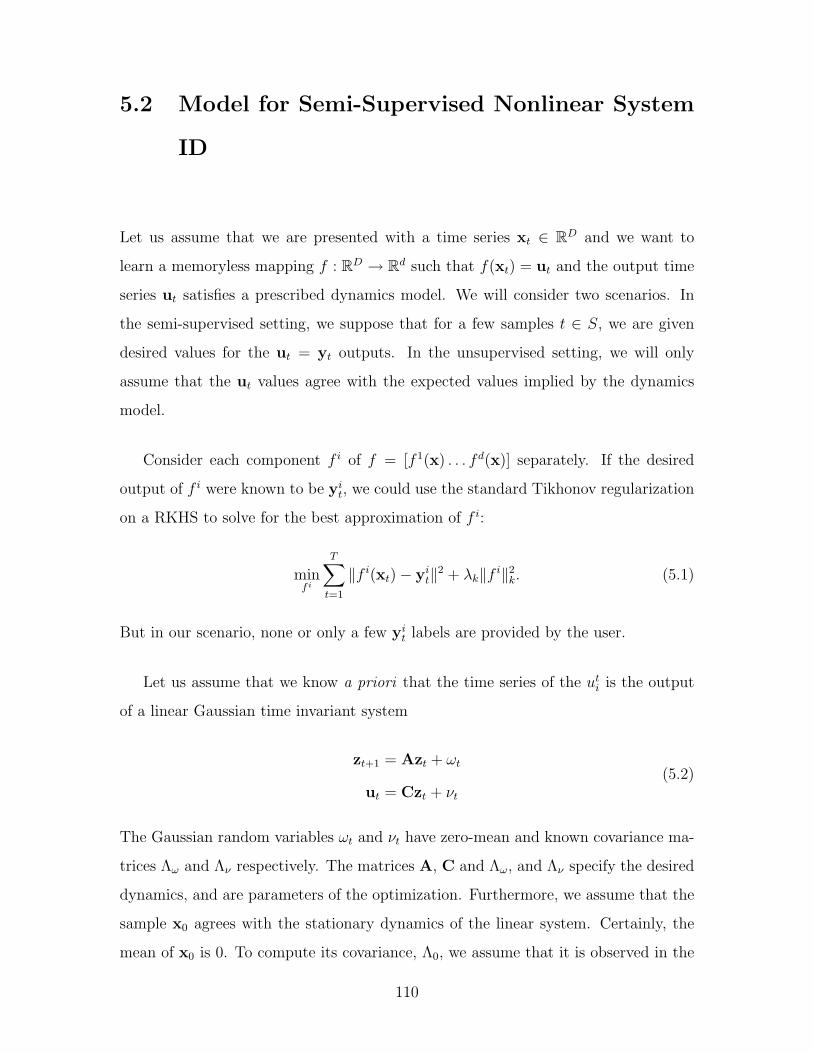
5.2 Model for Semi-Supervised Nonlinear System
ID
Let us assume that we are presented with a time series xt ∈ RD and we want to
learn a memoryless mapping f : RD → Rd such that f(xt) = ut and the output time
series ut satisfies a prescribed dynamics model. We will consider two scenarios. In
the semi-supervised setting, we suppose that for a few samples t ∈ S, we are given
desired values for the ut = yt outputs. In the unsupervised setting, we will only
assume that the ut values agree with the expected values implied by the dynamics
model.
Consider each component f i of f = [f 1(x) . . . fd(x)] separately. If the desired
output of f i were known to be yit, we could use the standard Tikhonov regularization
on a RKHS to solve for the best approximation of f i:
minf i
T∑t=1
‖f i(xt)− yit‖2 + λk‖f i‖2
k. (5.1)
But in our scenario, none or only a few yit labels are provided by the user.
Let us assume that we know a priori that the time series of the uti is the output
of a linear Gaussian time invariant system
zt+1 = Azt + ωt
ut = Czt + νt
(5.2)
The Gaussian random variables ωt and νt have zero-mean and known covariance ma-
trices Λω and Λν respectively. The matrices A, C and Λω, and Λν specify the desired
dynamics, and are parameters of the optimization. Furthermore, we assume that the
sample x0 agrees with the stationary dynamics of the linear system. Certainly, the
mean of x0 is 0. To compute its covariance, Λ0, we assume that it is observed in the
110
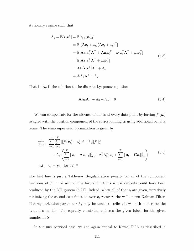
stationary regime such that
Λ0 = E[ztz>t ] = E[zt+1z
>t+1]
= E[(Azt + ωt)(Azt + ωt)>]
= E[Aztz>t A> + Aztω
>t + ωtz
>t A> + ωtω
>t ]
= E[Aztz>t A> + ωtω
>t ]
= AE[ztz>t ]A> + Λω
= AΛ0A> + Λω
(5.3)
That is, Λ0 is the solution to the discrete Lyapunov equation
AΛ0A> − Λ0 + Λω = 0 (5.4)
We can compensate for the absence of labels at every data point by forcing f i(xt)
to agree with the position component of the corresponding ut using additional penalty
terms. The semi-supervised optimization is given by
minf,u,z
d∑i=1
T∑t=1
‖f i(xt)− uit‖2 + λk‖f i‖2
k
+ λd
(T∑
t=2
‖zt −Azt−1‖2Λω
+ z>1 Λ−10 z1 +
T∑t=1
‖ut −Czt‖2Λν
)s.t. ut = yt for t ∈ S
(5.5)
The first line is just a Tikhonov Regularization penalty on all of the component
functions of f . The second line favors functions whose outputs could have been
produced by the LTI system (5.27). Indeed, when all of the ut are given, iteratively
minimizing the second cost function over zt recovers the well-known Kalman Filter.
The regularization parameter λd may be tuned to reflect how much one trusts the
dynamics model. The equality constraint enforces the given labels for the given
samples in S.
In the unsupervised case, we can again appeal to Kernel PCA as described in
111
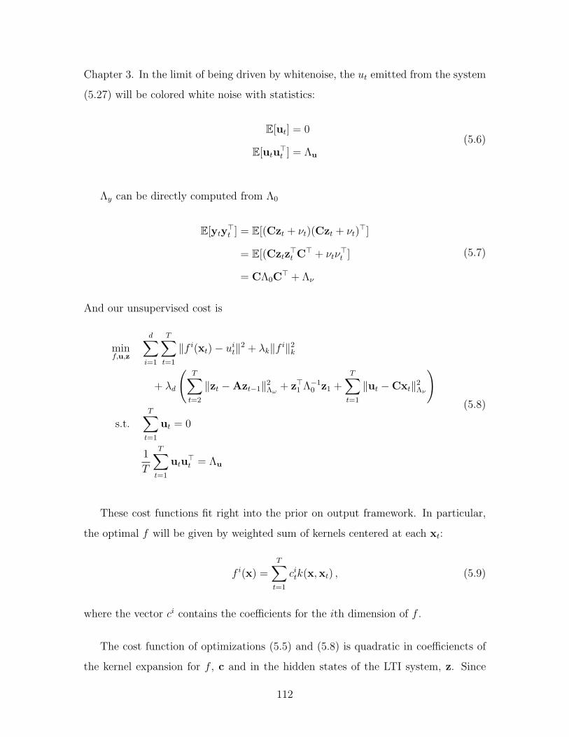
Chapter 3. In the limit of being driven by whitenoise, the ut emitted from the system
(5.27) will be colored white noise with statistics:
E[ut] = 0
E[utu>t ] = Λu
(5.6)
Λy can be directly computed from Λ0
E[yty>t ] = E[(Czt + νt)(Czt + νt)
>]
= E[(Cztz>t C> + νtν
>t ]
= CΛ0C> + Λν
(5.7)
And our unsupervised cost is
minf,u,z
d∑i=1
T∑t=1
‖f i(xt)− uit‖2 + λk‖f i‖2
k
+ λd
(T∑
t=2
‖zt −Azt−1‖2Λω
+ z>1 Λ−10 z1 +
T∑t=1
‖ut −Cxt‖2Λν
)
s.t.T∑
t=1
ut = 0
1
T
T∑t=1
utu>t = Λu
(5.8)
These cost functions fit right into the prior on output framework. In particular,
the optimal f will be given by weighted sum of kernels centered at each xt:
f i(x) =T∑
t=1
citk(x,xt) , (5.9)
where the vector ci contains the coefficients for the ith dimension of f .
The cost function of optimizations (5.5) and (5.8) is quadratic in coefficiencts of
the kernel expansion for f , c and in the hidden states of the LTI system, z. Since
112

these quantities are unconstrained, we can minimize the cost function directly. Let
S(u) := minf,z
d∑i=1
T∑t=1
‖f i(xt)− yit‖2 + λk‖f i‖2
k
+ λd
(T∑
t=2
‖zt −Azt−1‖2Λω
+ z>1 Λ−10 z1 +
T∑t=1
‖ut −Cxt‖2Λν
)(5.10)
We will now show that S(u) is a positive definite quadratic form in y. Indeed, we can
split this cost in half:
S(u) = minf
d∑i=1
T∑t=1
‖f i(xt)− uit‖2 + λk‖f i‖2
k
+ λd minz
(T∑
t=2
‖zt −Azt−1‖2Λω
+ z>1 Λ−10 z1 +
T∑t=1
‖ut −Cxt‖2Λν
)=: T (u) +K(u)
(5.11)
We have shown that
T (y) = λr
d∑i=1
yi>(K + λr11)−1yi (5.12)
The second term can also be written down explicitly. First, define the NT × NT
matrices
A :=
A −11 0 · · ·
0 A −11 0 · · ·. . .
0 · · · 0 A −11
0 · · · 0 0 11
Λ := diag(11T−1 ⊗ Λω, Λ0)
(5.13)
113

and note
K(u) = minz
u
z
> 11⊗ Λ−1ν 11T ⊗ (Λ−1
ν C)
11T ⊗ (C>Λ−1ν ) AΛ−1A + 11T ⊗ (C>Λ−1
ν C)
u
z
= u>
(11⊗ Λ−1
ν − 11T ⊗ (Λ−1ν C)(AΛ−1A + 11T ⊗ (C>Λ−1
ν C))−111T ⊗ (C>Λ−1ν ))
u
= u>(11T ⊗ Λ + (11T ⊗C)(AΛ−1A)−1(11T ⊗C>)
)−1
u .
(5.14)
The first equality is the standard solution to the quadratic program, and the sec-
ond equality follows from the matrix inversion lemma. Both results are derived in
Appendix A.
While this cost function looks a bit unwieldy, we can simplify it by realizing that
the quadratic form is nothing more than the inverse of the joint covariance of the ut
Λu :=(11T ⊗ Λν + (11T ⊗C)(AΛ−1A)−1(11T ⊗C>)
)(5.15)
In turn, we can use the Gaussian statistics of the LTI system to compute Λu
Proposition 5.2.1 Λu is a symmetric, positive-definite, block Toeplitz matrix and
for s ≥ t
Λust = CAs−tΛ0C
> + δstΛν (5.16)
Proof Since
E[usu>t ] = CE[xsx
>t ]C> + δstΛν (5.17)
we need only compute E[xsx>t ]. Suppose without loss of generality that s ≥ t
xt =t∑
j=0
At−jωjxs =s∑
k=t+1
As−kωk + As−txt (5.18)
Since ωk is i.i.d, E[xsxt] = E[As−txtxt] = As−tE[xtxt] = As−tΛ0. This proves the
proposition.
114

We may now combine the two quadratic forms to yield a joint optimization over
u
S(u) = λru> (K⊗ 11d + λr11dT ))−1 u + λdu
>Λu−1u =: u>Su (5.19)
where S is the sum of two positive definite quadratic forms and is hence positive
definite. In this regard, it now becomes apparent how to solve for the u labels.
In the semi-supervised case, we will be minimizing a positive definite quadratic
form over a subset of the ut with those ut with t ∈ S held fixed. This amounts to
solving a system of linear equations. We will present a fast method to solve this
particular system in the next section.
In the unsupervised case, we minimize a positive definite quadratic form subject
to a linear constraint forcing the ut to be zero mean and a set of quadratic constraints
enforcing the second moments of the individual ut variables. We will see that this
problem can be solved as an eigenvalue problem when we assume that the hidden
dynamical system is composed of d independent Markov chains.
Note that in both cases, we first recover the labels u. The function f mapping x’s
to u’s can be found by setting ci = (K + λ11T )ui.
5.2.1 Semi-supervised Algorithm
Under the constraints that ut = yt for t ∈ S, we may partition the vector u into
the labelled components and the unlabelled components: u =: [yLuU ]. That is, yL
denotes the vector composed of all the yt with t ∈ S stacked on top of each other
and uU denotes the vector composed of all the unlabelled points with t 6∈ S. We
may minimize the quadratic cost with respect to uU and holding yL fixed giving the
well-known least squares solution
u∗U = −S−1UUSULyL (5.20)
Indeed, a direct algorithm for solving the semi-supervised problem would be to
compute the matrix S, and then compute this quantity. For large T and d, this
115

requires four matrix inverses each of size Td which may be undesirable. Here we
present an algorithm that is much faster in practice.
First note that we can write
minu1,u2
u1
yL
u2
yL
> λr (K⊗ 11d + λr11dT )−1 0
0 λdΛu−1
u1
yL
u2
yL
s.t. u1 = u2
(5.21)
Introducing a Lagrange multiplier β to enforce the equality constraint, gives the
Lagrangian
L =
u1
yL
u2
yL
> λr (K⊗ 11d + λr11dT )−1 0
0 λdΛu−1
u1
yL
u2
yL
+ β(u1 − u2) (5.22)
Minimizing with respect to u1 and u2 gives
u1 = u1 +1
λr
[(K⊗ 11d + λr11dT )−1]−1UUβ
u2 = u1 −1
λd
[Λ−1y ]−1
UUβ
u1 = [(K⊗ 11d + λr11dT )−1]−1UU [(K⊗ 11d + λr11dT )−1]ULyL
u2 = [Λy−1]−1UU [Λu−1]ULyL
(5.23)
That is, u1 is the solution to the Tikhonov regularization problem adjusted by the
Lagrange multiplier term. u2 is the estimation of the outputs of the LTI system
also adjusted by a Lagrange multiplier term. We can simplify these equations by
employing the formula for the inverses of partitioned matrices found in Appendix A
116

and rewriting the last two lines as
u1 = [K⊗ 11d + λr11dT ]UL[K⊗ 11d + λr11dT ]−1LLyL
u2 = ΛyULΛy
LL−1
yL
(5.24)
We can solve for β by setting u1 = u2
β = (1
λR
[(K⊗ 11d + λr11dT )−1]−1UU +
1
λD
[Λ−1y ]−1
UU)−1(u2 + u1)
= (1
λR
(K⊗ 11d + λr11dT |U) +1
λD
(Λy|U))−1(u2 + u1)(5.25)
where (A|U) denotes the Schur complement AUU −AULA−1LLALU .
Thus, the algorithm works by first solving for yi, then computing the Lagrange
multiplier, and then adjusting the initial estimates. The first step is a least squares
problem with a matrix inversion of size |S| and a matrix multiplication of size |S| −
T × T . The second step requires computing Schur complements and solving a |S| −
T×|S|−T system of linear equations. Finally, the correction step involves a system of
equations with one of the Schur complements, and is again solving a |S|−T ×|S|−T
system of linear equations. Overall, this procedure is more efficient than directly
computing the quadratic form S that requires computing explicit matrix inverses.
5.2.2 Unsupervised Algorithm
In the case of the unsupervised algorithm, we will now present an eigenvalue problem
for when the underlying model consists of d independent Markov chains with one-
dimensional outputs. In this case, we can compute cost function for each chain
independently, and sum them together to yield the joint optimization
minu
d∑i=1
ui> (λr(K + λr11)−1 + λdT−1)ui
s.t.∑
t
ut = 0
∑t
utu>t = α11
(5.26)
117

ggg
st st+1 st+2A A
xt xt+1 xt+2
… …
Figure 5-1: A generative model for a linear system with nonlinear output. The states st arelow-dimensional representations lifted to high dimensional observables xt by an embeddingg.
This can be solved with an iterative eigenvalue solver as follows. First compute
the matrix A = (λr(K + λr11)−1 + λdT−1)−1. Then, ensure that ui has zero mean,
compute the projection onto the zero-mean subspace P := 11 − 11>/T . Then the d
largest eigenvalues of PAP are the optimal assignments for ui.
5.3 Relation to System Identification
Figure 5-1 depicts a standard generative model for time series generated by observing
a Markov chain with a nonlinear objective function. The latent state evolves according
to some Markov chain of states zt, t = 1 . . . T . At each time step, a nonlinear function
g : Rd → RD maps a linear function of the state yt = Czt to a D dimensional output
vector xt. Effects not accounted for by g are modeled as iid noise modifying the
output of g.
Learning the parameters of this generative model from a sequence of observations
y1, . . . ,yT can be computationally expensive [34, 98] even when the dynamics of the
hidden Markov chain are known. Instead of solving for g in this generative model, we
recover a projection function f : RD → Rd that maps images to their low-dimensional
representation in a random field. This random field consists of a function f that
maps the sequence of observed images to a sequence in Rd that evolves in accordance
with a Markov chain. The random field mirrors the generative model of Figure
5-1 by modeling the interactions between a Markov chain, the observations, and
supervised points provided by the user. Figure 5-2 depicts a random field describing
118
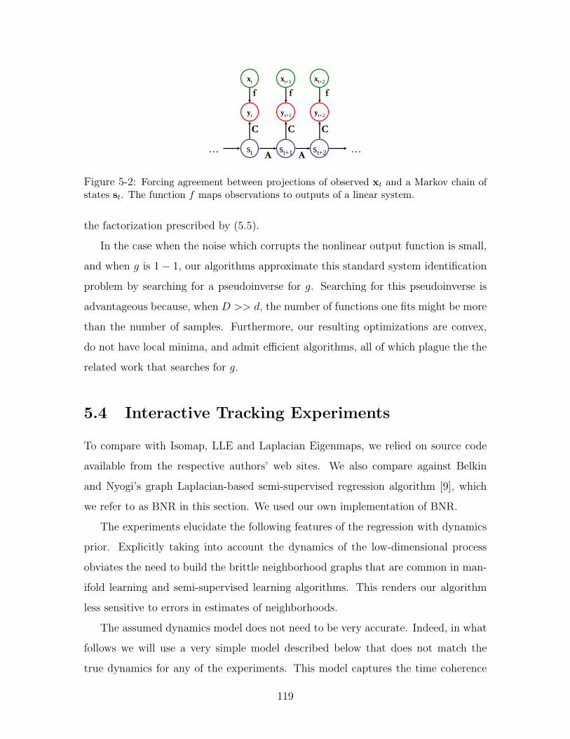
st st+1 st+2
yt yt+1 yt+2
A A
C C C
xt xt+1 xt+2
f f f
… …
Figure 5-2: Forcing agreement between projections of observed xt and a Markov chain ofstates st. The function f maps observations to outputs of a linear system.
the factorization prescribed by (5.5).
In the case when the noise which corrupts the nonlinear output function is small,
and when g is 1− 1, our algorithms approximate this standard system identification
problem by searching for a pseudoinverse for g. Searching for this pseudoinverse is
advantageous because, when D >> d, the number of functions one fits might be more
than the number of samples. Furthermore, our resulting optimizations are convex,
do not have local minima, and admit efficient algorithms, all of which plague the the
related work that searches for g.
5.4 Interactive Tracking Experiments
To compare with Isomap, LLE and Laplacian Eigenmaps, we relied on source code
available from the respective authors’ web sites. We also compare against Belkin
and Nyogi’s graph Laplacian-based semi-supervised regression algorithm [9], which
we refer to as BNR in this section. We used our own implementation of BNR.
The experiments elucidate the following features of the regression with dynamics
prior. Explicitly taking into account the dynamics of the low-dimensional process
obviates the need to build the brittle neighborhood graphs that are common in man-
ifold learning and semi-supervised learning algorithms. This renders our algorithm
less sensitive to errors in estimates of neighborhoods.
The assumed dynamics model does not need to be very accurate. Indeed, in what
follows we will use a very simple model described below that does not match the
true dynamics for any of the experiments. This model captures the time coherence
119
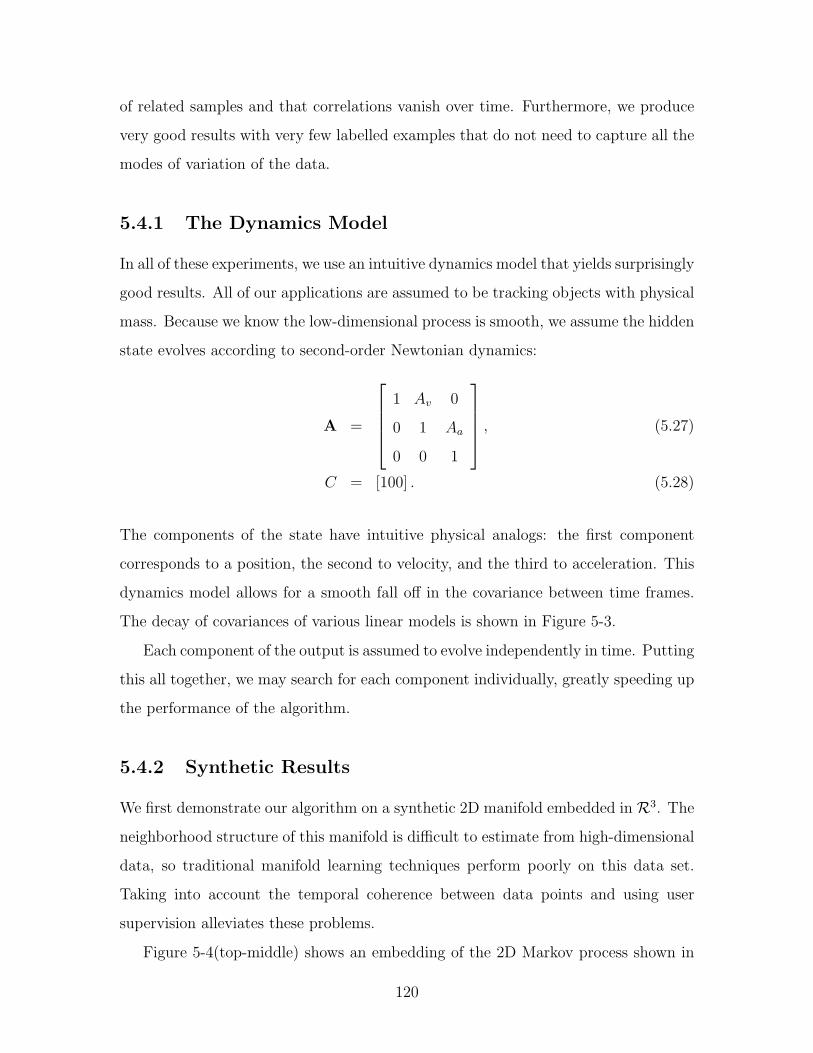
of related samples and that correlations vanish over time. Furthermore, we produce
very good results with very few labelled examples that do not need to capture all the
modes of variation of the data.
5.4.1 The Dynamics Model
In all of these experiments, we use an intuitive dynamics model that yields surprisingly
good results. All of our applications are assumed to be tracking objects with physical
mass. Because we know the low-dimensional process is smooth, we assume the hidden
state evolves according to second-order Newtonian dynamics:
A =
1 Av 0
0 1 Aa
0 0 1
, (5.27)
C = [100] . (5.28)
The components of the state have intuitive physical analogs: the first component
corresponds to a position, the second to velocity, and the third to acceleration. This
dynamics model allows for a smooth fall off in the covariance between time frames.
The decay of covariances of various linear models is shown in Figure 5-3.
Each component of the output is assumed to evolve independently in time. Putting
this all together, we may search for each component individually, greatly speeding up
the performance of the algorithm.
5.4.2 Synthetic Results
We first demonstrate our algorithm on a synthetic 2D manifold embedded in R3. The
neighborhood structure of this manifold is difficult to estimate from high-dimensional
data, so traditional manifold learning techniques perform poorly on this data set.
Taking into account the temporal coherence between data points and using user
supervision alleviates these problems.
Figure 5-4(top-middle) shows an embedding of the 2D Markov process shown in
120
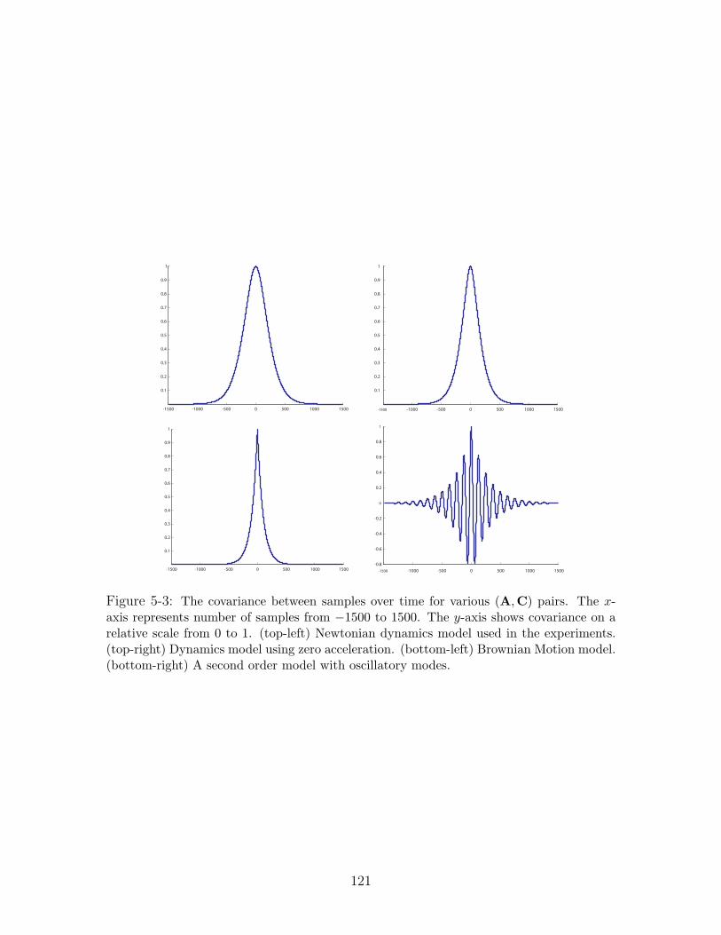
-1500 -1000 -500 0 500 1000 1500
0.1
0.2
0.3
0.4
0.5
0.6
0.7
0.8
0.9
1
-1500 -1000 -500 0 500 1000 1500
0.1
0.2
0.3
0.4
0.5
0.6
0.7
0.8
0.9
1
-1500 -1000 -500 0 500 1000 1500
0.1
0.2
0.3
0.4
0.5
0.6
0.7
0.8
0.9
1
-1500 -1000 -500 0 500 1000 1500
-0.8
-0.6
-0.4
-0.2
0
0.2
0.4
0.6
0.8
1
Figure 5-3: The covariance between samples over time for various (A,C) pairs. The x-axis represents number of samples from −1500 to 1500. The y-axis shows covariance on arelative scale from 0 to 1. (top-left) Newtonian dynamics model used in the experiments.(top-right) Dynamics model using zero acceleration. (bottom-left) Brownian Motion model.(bottom-right) A second order model with oscillatory modes.
121
0 0.5 1 1.5 2 2.5 3 3.5 4 4.5 5−3
−2
−1
0
1
2
3
12
34
0.511.522.5
−0.8
−0.6
−0.4
−0.2
0
0.2
0.4
0.6
0.8
yx
z
0 0.5 1 1.5 2 2.5 3 3.5 4 4.5 5−3
−2
−1
0
1
2
3
0 0.5 1 1.5 2 2.5 3 3.5 4 4.5 5−3
−2
−1
0
1
2
3
24
0.511.522.5
−0.8
−0.6
−0.4
−0.2
0
0.2
0.4
0.6
0.8
yx
z
0 0.5 1 1.5 2 2.5 3 3.5 4 4.5 5−3
−2
−1
0
1
2
3
Figure 5-4: (top-left) The true 2D parameter trajectory. Semi-supervised points are markedwith big black triangles. The trajectory is sampled at 1500 points (small markers). Pointsare colored according to their y-coordinate on the manifold. (top-middle) Embedding of apath via the lifting F (x, y) = (x, |y|, sin(πy)(y2 + 1)−2 + 0.3y). (top-right) Recovered low-dimensional representation using our algorithm. The original data in (top-left) is correctlyrecovered. (bottom-left) Even sampling of the rectangle [0, 5] × [−3, 3]. (bottom-middle)Lifting of this rectangle via F . (bottom-right) Projection of (bottom-middle) via the learnedfunction g. g has correctly learned the mapping from 3D to 2D. These figures are best viewedin color.
−0.6 −0.4 −0.2 0 0.2 0.4 0.6 0.8
−0.4
−0.2
0
0.2
0.4
0.6
0 1 2 3 4 5−3
−2
−1
0
1
2
3
Figure 5-5: (left) Isomap’s projection into R2 of the data set of Figure 5-4(top-middle).Errors in estimating the neighborhood relations at the neck of the manifold cause theprojection to fold over itself. (right) Projection with BNR, a semi-supervised regressionalgorithm. There is no folding, but the projections are not close to the ground truth shownin Figure 5-4(top-left).
122
Figure 5-4(top-left) into R3. The semi-supervised points are marked with a large tri-
angle. Figure 5-4(top-right) shows our interpolated results for the unlabelled points.
The interpolated values are close to the true values that generated the data set. Al-
though the process is smooth, it clearly does not follow the dynamics assumed by
Equation (5.27) because it bounces off the boundaries of the rectangle [0, 5]× [−3, 3].
Nevertheless, the assumed dynamics of Equation (5.27) are sufficient for recovering
the true location of unlabelled points.
To assess the quality of the learned function g on as-yet unseen points, we evenly
sampled the 2D rectangle [0, 5]× [−3, 3] and lifted the samples to R3 using the same
mapping used to generate the training sequence. See Figure 5-4(bottom-left and
bottom-right). Each sample inR3 is passed through g to obtain the 2D representation
shown in Figure 5-4(bottom-right). The projections fall close to the true 2D location
of these samples.
We applied LLE, Laplacian Eigenmaps, and Isomap to the data set of Figure 5-
4(top-middle). Isomap produced the result shown in Figure 5-5(left). It is difficult to
estimate the neighborhood structure near the neck, where the manifold comes close
to intersecting itself, so Isomap creates folds in the projection.
Figure 5-5(right) shows the result of BNR. Compared to our result in Figure 5-
4(top-right), the interpolated results are incorrect for most points. Since BNR does
not attempt to enforce any geometric invariance in the projection, it is fairly robust
to the neighborhood estimation problem.
For this and subsequent data sets, neither LLE nor Laplacian Eigenmaps produced
sensible results. This may be due to the low rate at which the manifold is sampled.
5.4.3 Interactive Tracking
Our algorithm is not limited to rigid body tracking. We applied it to a lip tracking
experiment exhibiting deformable motion, and to an upper-body tracking experiment
exhibiting articulated motion. In these experiments, we restricted ourselves to re-
covering the missing labels of the training data and labeling frames acquired under
the same setting from which the training data was gathered. Our algorithm op-
123

erates on the entire frames, as shown in the figures. Images were not in any way
preprocessed before applying our algorithm, though to apply the learned mapping to
different settings, more taylored representations or kernels could be employed. We
tuned the parameters of our algorithm (Av, Aa, the diagonal entries of Λω, and the
weights λd, λs, and λk) by minimizing the leave-one-out cross validation error on the
semi-supervised points using the simplex method.
Figure 5-6 shows frames in a 2000 frame sequence of a subject articulating his lips.
The top row shows the frames that were manually annotated with a bounding box
around the lips. The bottom row shows the bounding boxes returned by g on some
typical frames in the sequence. Only five labelled frames were necessary to obtain
good lip tracking performance. The tracker is robust to natural changes in lighting,
blinking, facial expressions, small movements of the head, and the appearance and
disappearance of teeth.
Figure 5-7 shows 12 labelled images in a 2300 frame sequence of a subject moving
his arms. These frames were manually labelled with line segments denoting the
upper and lower arms. Figure 5-8 shows the recovered limb positions for unlabelled
samples, some of which were not in the training sequence. Because the raw pixel
representation is used, there are very few visual ambiguities between appearance and
pose, and occlusions due to crossing arms do not present a problem.
The utility of dynamics is most apparent in articulated tracking. Setting λd to
zero makes our algorithm ignore dynamics, forcing it to regress on the semi-supervised
examples only. The resulting function produced the limb locations shown in black in
Figure 5-8. Using dynamics allows the system to take advantage of the unsupervised
points, producing better estimates of limb position.
5.4.4 Calibration of HCI Devices
The Audiopad is an interface for musical performance that aims to combine the mod-
ularity of knob based controllers with the expressive character of multidimensional
tracking interfaces [75]. Audiopad uses a series of electromagnetically tracked objects,
called pucks, as input devices. The performer assigns each puck to a set of samples
124

Figure 5-6: The bounding box of the mouth was annotated for 5 frames of a 2000 framevideo. The labelled points (shown in the top row) and first 1500 frames were used totrain our algorithm. The images were not altered in any way before computing the kernel.The parameters of the model were fit using leave-one-out cross validation on the labelleddata points. Plotted in the second row are the recovered bounding boxes of the mouth forvarious frames. The first three examples correspond to unlabelled points in the trainingset. The tracker is robust to natural changes in lighting, blinking, facial expressions, smallmovements of the head, and the appearance and disappearance of teeth.
Figure 5-7: The twelve supervised points in the training set for articulated hand tracking(see Figure 5-8).
125
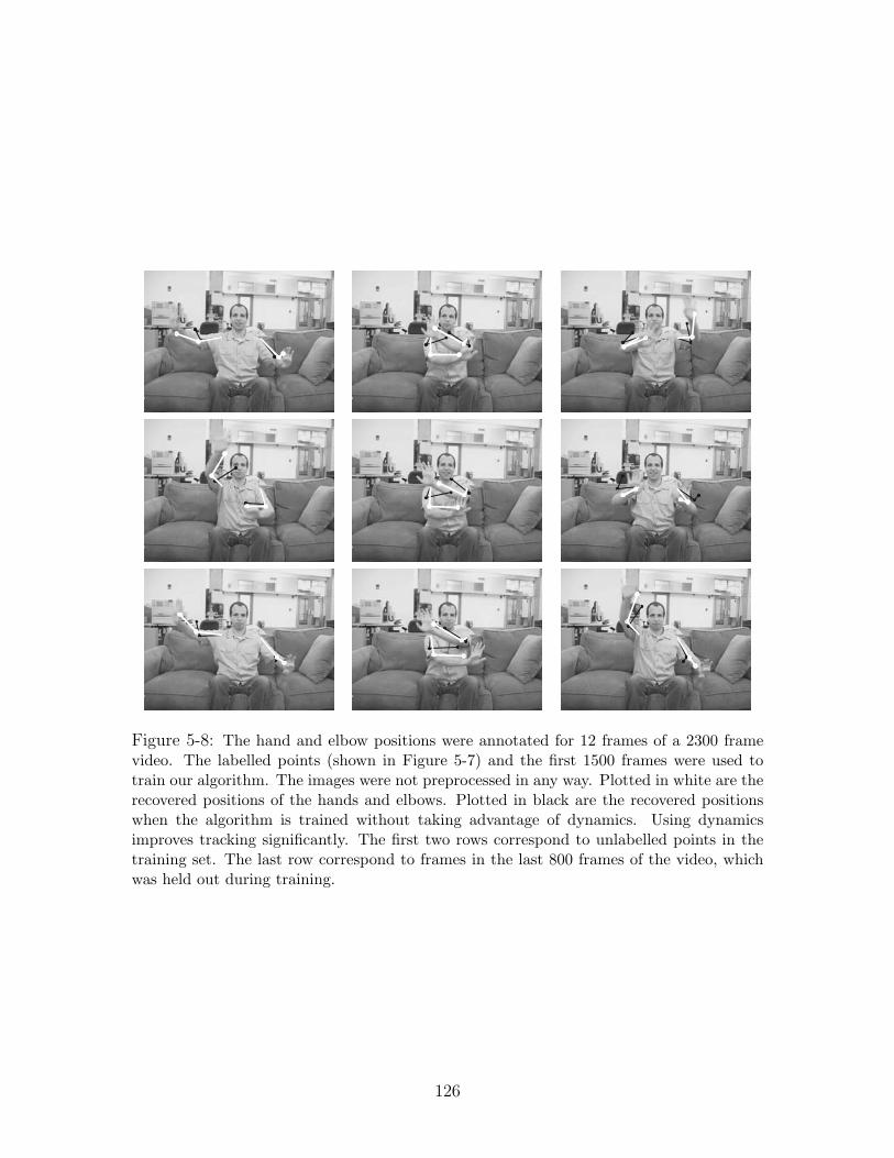
Figure 5-8: The hand and elbow positions were annotated for 12 frames of a 2300 framevideo. The labelled points (shown in Figure 5-7) and the first 1500 frames were used totrain our algorithm. The images were not preprocessed in any way. Plotted in white are therecovered positions of the hands and elbows. Plotted in black are the recovered positionswhen the algorithm is trained without taking advantage of dynamics. Using dynamicsimproves tracking significantly. The first two rows correspond to unlabelled points in thetraining set. The last row correspond to frames in the last 800 frames of the video, whichwas held out during training.
126
that he wishes to control. Audiopad determines the position and orientation of these
objects on a tabletop surface and maps this data into musical cues such as volume
and effects parameters. Graphical information is projected onto the tabletop surface
from above, so that information corresponding to a particular physical object on the
table appears directly on and around the object.
The Audiopad hardware is a result of further development of the Sensetable sys-
tem [74]. The Sensetable tracks each puck using one or two RF tags. A simple type
of RF tag, known as an LC tag, consists of a coil of wire and a capacitor. This circuit
resonates at a specific frequency depending on its inductance and capacitance. Using
clever antenna geometries, these simple structures can be tracked in space using am-
plitude measurements of the tags resonant frequencies. To determine the position of
the RF tag on a two dimensional surface, a modified version of the sensing apparatus
found in the ZowieTMEllie’s Enchanted GardenTMplay set is used [21]. Each tag on
the table resonates at a different frequency, so their positions can be determined inde-
pendently, but there is a fair amount of black art in the decoding of the amplitude of
resonances in the antenna to the tag-positions. As an exemplary embodiment, I will
now describe how to learn the mapping from antenna resonance to tag position using
semi-supervised regression with no knowledge of the particularities of the antenna
geometry.
We wish to learn to map these 10 recorded measurments to the 2D position of the
RFID tag. Previously, a mapping was recovered by hand through an arduous reverse-
engineering process that involved building a physical model of the inner-workings
of the Sensetable, and resorting to trial and error to refine the resulting mappings.
Rather than reverse-engineering this device by hand, we show that it is possible to
recover these mappings semi-automatically, with only 4 labelled examples and some
unlabelled data points. This is a challenging task because the relationship between
the tags position an the observed measurements is highly oscillatory. Once it is
learned, we can use the mapping to track RFID tags. Of course, this procedure is
quite general, and can be applied to a variety of other hardware.
To collect labelled examples, we placed the tag on each of the four corners of
127

the Sensetable and recorded the Sensetables output. We collected unlabelled data
by sweeping the tag on the Sensetables surface for about 400 seconds, and down-
sampled the result by a factor of 3 to obtain about 3600 unlabelled data points. The
four labelled points, along with the few minutes of recorded data were passed to the
semi-supervised learning algorithm to recover the mapping. Figure 5-10(left) shows
the ground truth trajectory of the RFID tag, as recovered by the manually reverse-
engineered Sensetable mappings. The four triangles in the corners of the figure depict
the location of the labelled examples. The rest of the 2D trajectory was not made
available to the algorithm. Figure 5-9(right) shows an example of the output from the
Sensetable. Contrary to what one might hope, each trace of the output does not have
a straightforward one-to-one relationship to a component of the 2D position. Rather,
this relationship is smooth but sinusoidal. For example, when the tag is moved in a
straight line from left to right, it generates sinusoidal traces similar to those shown
in Figure 5-9(right).
The algorithm took 90 seconds to process this data set on a 2.8 Ghz Xeon machine.
The trajectory is recovered accurately despite the complicated relationship between
the 10 outputs and the tag position. See Figure 6. Its RMS distance to the ground
truth trajectory is about 1.3 cm, though the ground truth itself is based on the reverse
engineered tracker and may be inaccurate.
The mapping from measurements to positions is learned can be used to track tags.
The recovered trajectories provide a subjective means of evaluating the accuracy of
the tracker. Individual samples of 10 measurements can be passed to f to recover the
corresponding tag position. Figure 5-11 shows the output of a few test paths. The
recovered trajectories match the patterns traced by the tag.
The mapping cannot be learned from the four labelled examples alone using
Tikhonov regularization, demonstrating that access to unlabelled data and prior
knowledge about dynamics is very helpful in real-world applications. See Figure 5-
12(left). Figure 5-12(middle) shows the trajectory recovered by BNR with its most
favorable parameter setting for this data set. Figure 5-12(right) shows the trajectory
recovered by BNR when temporally adjacent neighbors are counted as part of the ad-
128

10 20 30 40 50 60
−100
−80
−60
−40
−20
0
20
40
60
80
100
Figure 5-9: An image of the Audiopad. The plot shows an example stream of antennaresonance information. Samples from the output of the Sensetable over a six second period,taken over the trajectory marked by large circles in the left panel.
jacency graph when computing the Laplacian. As with the synthetic data set, there
is severe shrinkage toward the mean of the labelled points, and some folding at the
bottom. Taking temporal adjacency into account does not significantly improve the
results.
5.4.5 Electric Field Imaging:
Anyone who has walked near a radio has likely noticed that the human body can cause
interference with the transmission. This is because the human body acts as a capacitor
coupling the radio frequencies to ground. This interference has been extensively
utilized in the design of human computer interfaces and musical instruments at the
Media Lab [33] [110] [72].
Some elementary field imaging sensor architectures have been developed by search-
ing complex forward models [92]. A different approach was to combine several simple
sensors [79]. Here I demonstrate a simple, inexpensive architecture based around a
resistive sheet connected to a simple network of sub-dollar microcontrollers.
The Resistofish is a resistive sheet with electrodes along each side (see Figure 5-
14). When a human is in the proximity of the sheet, it couples capacitively to the
sheet. Based on the position of the body, there is a resistance between the coupling
point and the electrodes. If one sensor is charged and another measures current with
low impedance, the charging time can be used to estimate the time constant of the
129

50 100 150 200 250 300 350 400 450
350
400
450
500
550
600
50 100 150 200 250 300 350 400 450
400
450
500
550
600
50 100 150 200 250 300 350 400 450
350
400
450
500
550
600
Figure 5-10: (left) The ground truth trajectory of the tag. The tag was moved aroundsmoothly on the surface of the Sensetable for about 400 seconds, producing about 3600signal strength measurement samples after downsampling. Triangles indicate the four lo-cations where the true location of the tag was provided to the algorithm. The color ofeach point is based on its y-value, with higher intensities corresponding to higher y-values.(right) (middle) The recovered tag positions match the original trajectory. (right) Errorsin recovering the ground truth trajectory. Circles depict ground truth locations, with theintensity and size of each circle proportional to the Euclidean distance between a pointstrue position and its recovered position. The largest errors are outside the bounding boxof the labelled points. Points in the center are recovered accurately, despite the lack oflabelled points there.
−450 −400 −350 −300 −250 −200 −150 −100 −50−650
−600
−550
−500
−450
−400
−350
−450 −400 −350 −300 −250 −200 −150 −100
−600
−550
−500
−450
−400
−350
−450 −400 −350 −300 −250 −200
−580
−560
−540
−520
−500
−480
−460
−440
−420
−400
−300 −250 −200 −150 −100 −50
−580
−560
−540
−520
−500
−480
−460
−440
−420
−400
−400 −350 −300 −250 −200 −150−600
−550
−500
−450
−400
−400 −350 −300 −250 −200 −150−600
−550
−500
−450
−400
−400 −350 −300 −250 −200 −150
−580
−560
−540
−520
−500
−480
−460
−440
−420
−400
−380
−400 −350 −300 −250 −200 −150 −100
−600
−550
−500
−450
−400
−350
Figure 5-11: Once f is learned, it can be used it to track tags. Each panel shows a groundtruth trajectory (blue crosses) and the estimated trajectory (red dots). The recoveredtrajectories match the intended shapes.
130

0 50 100 150 200 250 300 350 400 450 500
350
400
450
500
550
600
100 150 200 250 300 350 400
350
400
450
500
550
600
100 150 200 250 300 350 400
350
400
450
500
550
600
Figure 5-12: (left) Tikhonov regularization with labelled examples only. The trajectory isnot recovered. (middle) BNR with a neighborhood size of three using nearest neighbors.(right) BNR with same neighborhood settings, with the addition of temporal neighbors.There is folding at the bottom of the plot, where black points appear under the red points,and severe shrinking towards the mean.
RC pair.
Using the four electrode pairs, we trained two hand trackers with the resistive
sheets. The first was made by creating a 7 × 12 grid on the sheet and measuring
approximately 30 samples per point. We then used leave-one-out cross validation
to train a kernel machine to map sensor outputs to hand positions. The second
tracker was made using the unsupervised regression algorithm with a dynamics prior.
Creating a similar 2D tracing, we learned the best mapping, with no parameter tuning
and 200 samples. The results of a test tracing are displayed in Figure 5-15.
Both algorithms recovered geometry to similar accuracy (see Figure 5-16), but
the supervised algorithm was far more laborious to train. While the unsupervised
method only took 30 seconds to acquire the data, and 10 seconds to process it, the
supervised algorithm took nearly an hour to gather the data, and an hour to perform
the cross validation.
5.5 Conclusion
We have presented a semi-supervised regression algorithm for learning the appearance
manifold of a scene from a video sequence. By taking advantage of the dynamics
in video sequences, our algorithm learns a function that projects images to a low-
dimensional space with semantically meaningful coordinate axes. The experiments
131
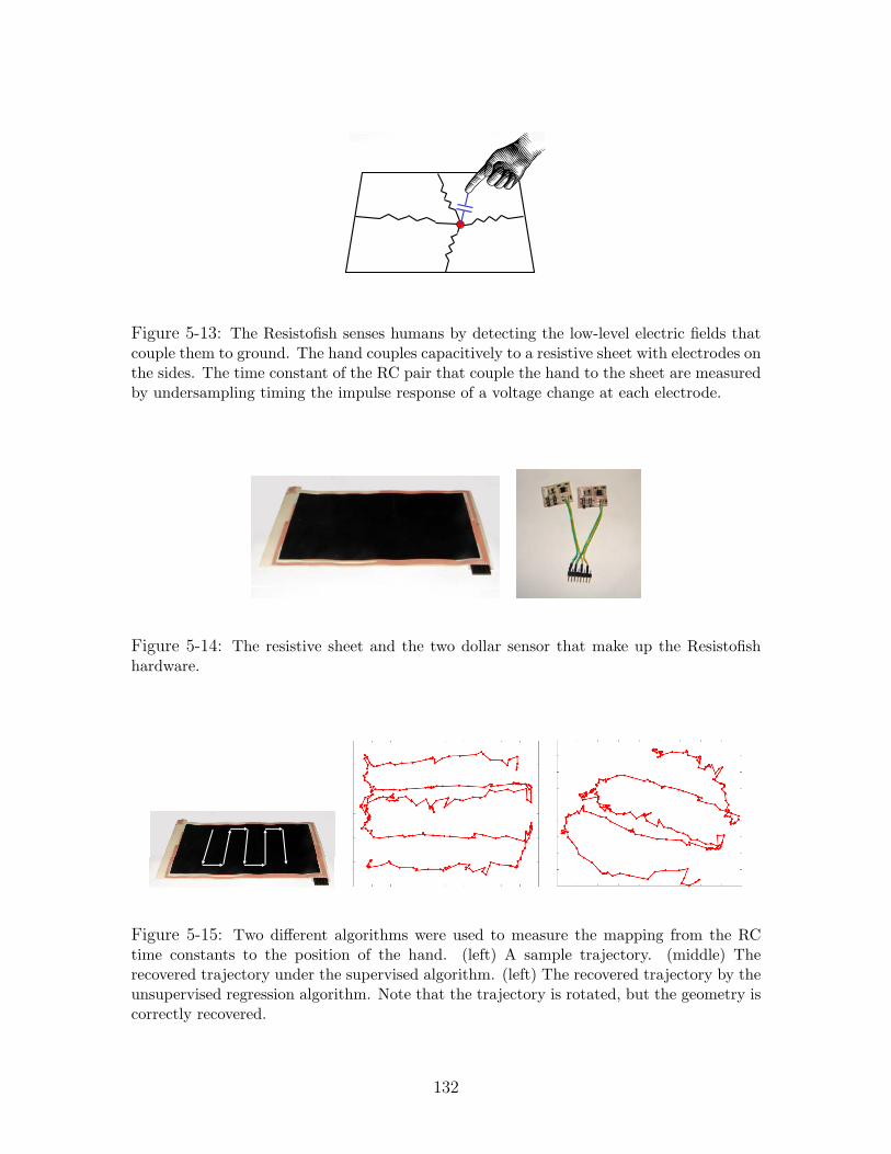
Learning to Track with Resistofish
$2
Impulse responseVoltage
time
Figure 5-13: The Resistofish senses humans by detecting the low-level electric fields thatcouple them to ground. The hand couples capacitively to a resistive sheet with electrodes onthe sides. The time constant of the RC pair that couple the hand to the sheet are measuredby undersampling timing the impulse response of a voltage change at each electrode.
Figure 5-14: The resistive sheet and the two dollar sensor that make up the Resistofishhardware.
Tikhonov Regularization. 12x7 grid. 2595 examples. All labels provided.
Unsupervised Algorithm. 200 examples. No labels. Figure 5-15: Two different algorithms were used to measure the mapping from the RC
time constants to the position of the hand. (left) A sample trajectory. (middle) Therecovered trajectory under the supervised algorithm. (left) The recovered trajectory by theunsupervised regression algorithm. Note that the trajectory is rotated, but the geometry iscorrectly recovered.
132

Figure 5-16: The top row is recovered using the supervised algorithm. The bottom rowis recovered by the unsupervised algorithm. The middle panels is the recovered traces ofsomeone writing ”MIT.” The right-most panels are the recovered traces of someone writing”Ben.” The mapping recovered by the unsupervised algorithm is as useful for trackinghuman interaction as the mapping recovered by the fully calibrated regression algorithm.
demonstrate that this optimization framework is a powerful way to build trackers
with very little domain specific knowledge and very few data points.
133

134

Chapter 6
Output Prior: Manifolds of Low
Codimension
In this final chapter, I will describe a novel algorithm for learning manifolds defined
by observed data. Most algorithms that claim to learn manifolds can only operate
under restrictive locality assumptions, and, even more problematically, can only learn
mappings that are 1-1 [97, 85, 8, 27, 106, 16]. The most simple example of a manifold,
the sphere, breaks all of the present algorithms.
Here, I take a different approach. I will learn functions on the high dimensional
space that are constant on the manifold. These functions will define the manifold
structure, with the space normal to the manifold spanned by the gradients of these
functions.
This method is similar to the novelty deteciton algorithms that use kernels to
generate inequality constraints that bound the data [96, 10, 88]. Here, we will learn
equality constraints, and in turn, implicitly defined manifolds on which the data lie.
135

6.1 Learning Manifolds of Low Codimension
Let M be a surface in embedded in Rd implicitly defined by unknown differentiable
functions f1, . . . , fJ . That is,
M = x ∈ Rd : fj(x) = 0 j = 1, . . . J (6.1)
Let us further assume that Dfj(x) span a J-dimensional space for every x ∈ M.
Such a surface is a manifold of codimension J by the implicit function theorem.
Let xi be a collection of N points sampled from M via some unknown probability
distribution p on M.
We assume that both p and f1, . . . , fJ are unknown. Let us even assume the
codimension J is unknown. The goal will be to approximate the unknown functions
fj from the data xi
(i) Lift the data to a higher dimensional Hilbert space H via a mapping Φ : Rd →
H.
(ii) Using linear algebra, find a set of vectors aj, j = 1, . . . , k such that a>j Φ(xi) = 0
for all i.
(iii) Return fj(x) := a>j Φ(x)
The only difficulty is in choosing the mapping Φ so that the output function is
stable and produces reasonable models. Following the theme of the thesis, we will
choose fj to live in a Reproducing Kernel Hilbert Space. There are two cases we
will investigate. First, we will discuss the case of finite dimensional liftings and, in
particular, consider the case when fj are polynomials. Then we will focus on the
generic case where fj live in an arbitrary RKHS.
What is the advantage of learning multiple functions which are zero on the data
set? And how many functions are needed to define an implicit surface? The answer
comes from a variant of the implicit function theorem which states that if g : Rd → RJ
with J ≤ d, then if if Dg has rank J at every x with g(x) = 0, then the preimage of
136

0 under g is a manifold of dimension d − J [41]. J is called the codimension of the
manifold. It is the codimension of the tangent space of the manifold in Rd for every
point x ∈M. The co-dimension is stable to small perturbations of the map g. That
is, Dg remains full rank even if g is perturbed by a small amount, and, in turn, the
preimage of 0 remains a d− J-dimensional manifold.
Let us now consider the situation where we have learned L functions gl which are
all identically zero on M. If L < J then the dimension of the zero-set of the gl is
of larger dimension than that of M. If on the other hand, L > J , we know that the
rank of Dg is at most J . In this case, we can use the rank of Dg to estimate the
codimension of the manifold and from this we can try to learn a set of J functions
which are zero only on M. In what follows, we will learn d + 1 functions, more than
could ever be necessary to define M. From these functions, we will estimate both the
codimension of M and the smallest set of functions necessary to describe M.
6.2 Basis Functions and Polynomial Models
The first option to consider is to choose a set of differentiable basis functions bα for
L2(Rd) and lift x to a subset of those functions
Φ(x) :=[
b1(x) · · · bT (x)]>
(6.2)
To compute a constraint, compute the SVD of the matrix A = [Φ(x1), . . . , Φ(xN)] If
A does not have full row rank, than any vector in the left null space will suffice for
the desired vector a.
For example, if we wanted the constraint to be algebraic, we could lift to a vector
of monomials of bounded degree
Φ
([x1 · · · xd
]>):=[
1 x1 · · · xd x1x2 x1x3 · · ·]>
. (6.3)
The utility of such an approach can be illustrated by supposing the data was drawn
137
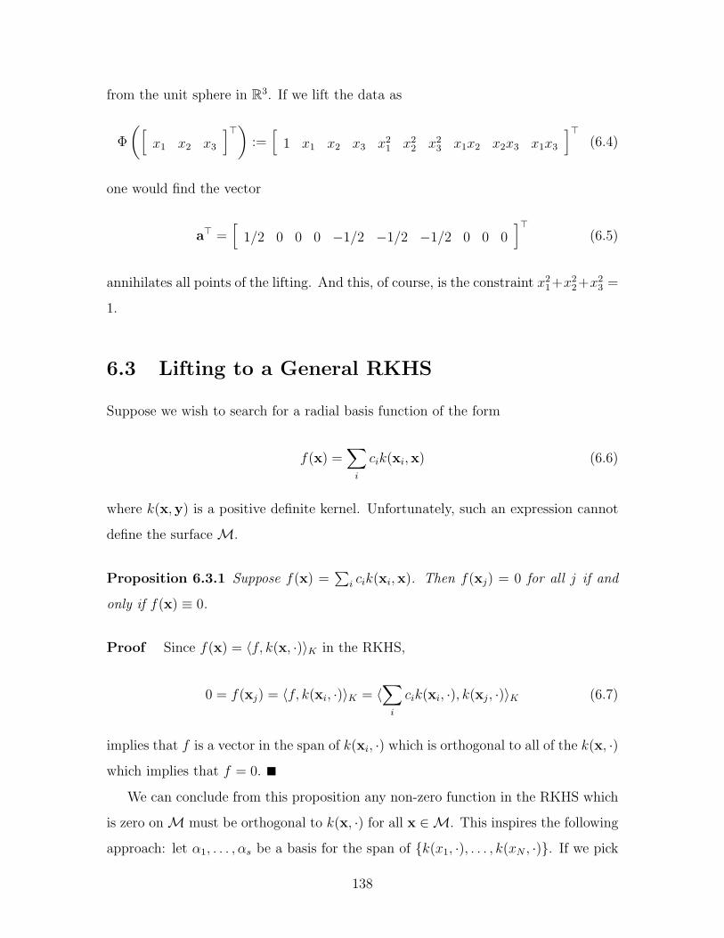
from the unit sphere in R3. If we lift the data as
Φ
([x1 x2 x3
]>):=[
1 x1 x2 x3 x21 x2
2 x23 x1x2 x2x3 x1x3
]>(6.4)
one would find the vector
a> =[
1/2 0 0 0 −1/2 −1/2 −1/2 0 0 0]>
(6.5)
annihilates all points of the lifting. And this, of course, is the constraint x21+x2
2+x23 =
1.
6.3 Lifting to a General RKHS
Suppose we wish to search for a radial basis function of the form
f(x) =∑
i
cik(xi,x) (6.6)
where k(x,y) is a positive definite kernel. Unfortunately, such an expression cannot
define the surface M.
Proposition 6.3.1 Suppose f(x) =∑
i cik(xi,x). Then f(xj) = 0 for all j if and
only if f(x) ≡ 0.
Proof Since f(x) = 〈f, k(x, ·)〉K in the RKHS,
0 = f(xj) = 〈f, k(xi, ·)〉K = 〈∑
i
cik(xi, ·), k(xj, ·)〉K (6.7)
implies that f is a vector in the span of k(xi, ·) which is orthogonal to all of the k(x, ·)
which implies that f = 0.
We can conclude from this proposition any non-zero function in the RKHS which
is zero on M must be orthogonal to k(x, ·) for all x ∈M. This inspires the following
approach: let α1, . . . , αs be a basis for the span of k(x1, ·), . . . , k(xN , ·). If we pick
138

some basis functions b1, . . . , bt in the RKHS which are not contained in the span of
the data, we can perform Gram-Schmidt on the set b1, . . . , bt, α1, . . . , αs to yield t
functions g1, . . . , gt which are orthonormal in the RKHS and are orthogonal to the
span of the data. We would then have gj(xi) = 0 for all i. And, in the limit of enough
data, we would have gj(x) = 0 for all x ∈M.
In practice, this amounts to fixing the expansion for gj as
gj(x) =t∑
m=1
ajmbm(x) +N∑
n=1
cjnk(xn,x) (6.8)
and searching for [a, c] such that gj(x) = 0. That is, searching in the null space of
the rows of
A = [Φ(x1), . . . , Φ(xN)] (6.9)
where
Φ(x) :=[
b1(x) · · · bt(x) k(x1,x) · · · k(xN ,x)]>
. (6.10)
There are thus two different interpretations of the lifting when using radial basis
functions. The first is that we have chosen a set of basis functions based on the data
x1, . . . ,xN and then lifted to this basis set as in Section 6.2. The second interpretation
is that we are lifting each data point to the infinite dimensional RKHS under the
mapping x 7→ k(x, ·) and are searching for an element in the RKHS orthogonal to
the data under this lifting.
6.4 Null Spaces and Learning Surfaces
Note that we could have tried to learn a set of functions gj such that
gj(xi) = gj(xk) ∀i, k (6.11)
This function would be constant on the data set. A function that is zero on the data
set could be produced by setting gj = gj − gj(x1).
139

Define the extended kernel matrix to be the N×(N + t) matrix K = [K,B] where
B has entries
Bij = bj(xi) (6.12)
For each M , define the (M − 1)×M matrix A[M ] to be
A[M ]ij =
1 1 ≤ i = j < M − 1
−1 1 ≤ i = j − 1 < M − 1
0 otherwise
(6.13)
that is
A[M ] =
1 −1 0 0 . . . 0
0 1 −1 0 . . . 0. . .
0 . . . 0 1 −1 0
0 . . . 0 0 1 −1
(6.14)
A function of the form (6.16) satisfies (6.15) for all i and k between 1 and N if and
only if A[N ]K[c, a]> = 0. In particular, the coefficients of the expansion in (6.16) lie
in the null space of A[N ]K. In this case, we can find the space of all functions that
are constant on the data set.
This approach has a nice generalization to the case where we are searching for a
function that is constant on multiple data sets. For example, if we are given multiple
trajectories of a conservative system, each trajectory will have constant energy, but
two different trajectories will likely have different energy.
In this case, we are presented with data partitioned into disjoint subsets Sk ⊂
1, . . . , N. We seek to find gj such that
gj(xm) = gj(xn) if m, n ∈ Sk for some k (6.15)
Assume without loss of generality, that each Sk is a contiguous subset of 1, . . . , N
of size Nk. In this case, we may define the matrix A = diag(A[N1], . . . ,A[Nk]) and
140
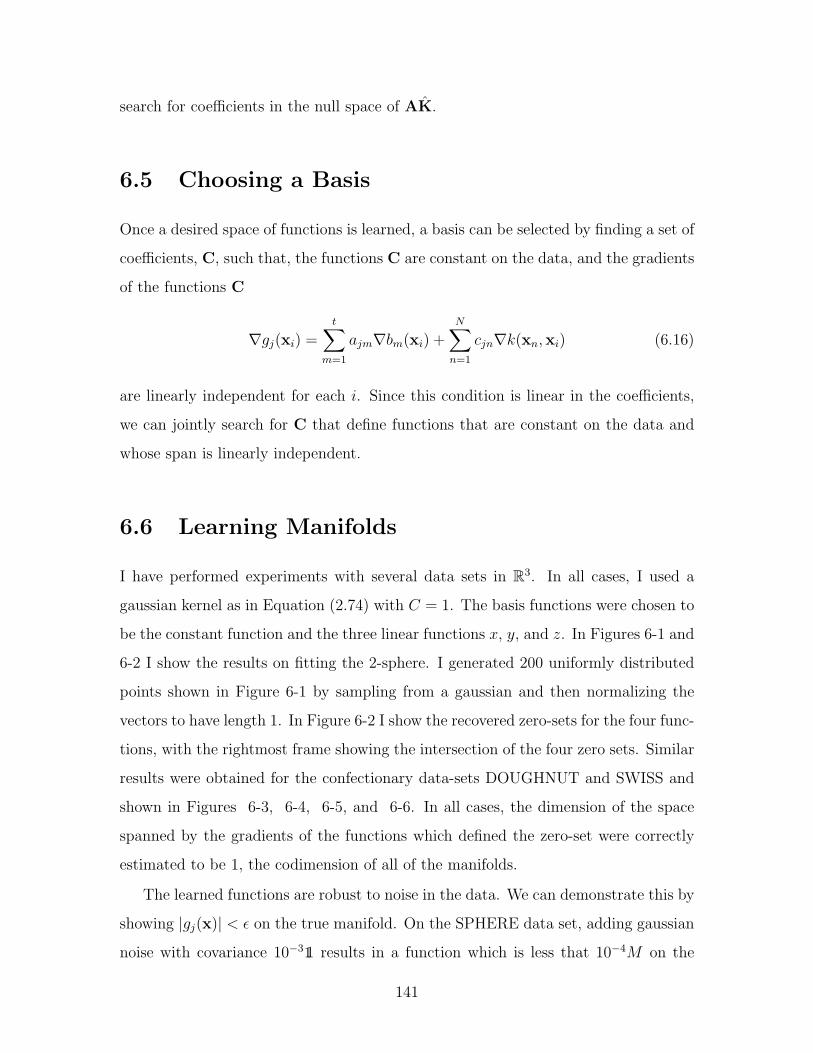
search for coefficients in the null space of AK.
6.5 Choosing a Basis
Once a desired space of functions is learned, a basis can be selected by finding a set of
coefficients, C, such that, the functions C are constant on the data, and the gradients
of the functions C
∇gj(xi) =t∑
m=1
ajm∇bm(xi) +N∑
n=1
cjn∇k(xn,xi) (6.16)
are linearly independent for each i. Since this condition is linear in the coefficients,
we can jointly search for C that define functions that are constant on the data and
whose span is linearly independent.
6.6 Learning Manifolds
I have performed experiments with several data sets in R3. In all cases, I used a
gaussian kernel as in Equation (2.74) with C = 1. The basis functions were chosen to
be the constant function and the three linear functions x, y, and z. In Figures 6-1 and
6-2 I show the results on fitting the 2-sphere. I generated 200 uniformly distributed
points shown in Figure 6-1 by sampling from a gaussian and then normalizing the
vectors to have length 1. In Figure 6-2 I show the recovered zero-sets for the four func-
tions, with the rightmost frame showing the intersection of the four zero sets. Similar
results were obtained for the confectionary data-sets DOUGHNUT and SWISS and
shown in Figures 6-3, 6-4, 6-5, and 6-6. In all cases, the dimension of the space
spanned by the gradients of the functions which defined the zero-set were correctly
estimated to be 1, the codimension of all of the manifolds.
The learned functions are robust to noise in the data. We can demonstrate this by
showing |gj(x)| < ε on the true manifold. On the SPHERE data set, adding gaussian
noise with covariance 10−311 results in a function which is less that 10−4M on the
141

−1.5−1
−0.50
0.51
1.5
−1.5−1
−0.50
0.51
1.5−1.5
−1
−0.5
0
0.5
1
1.5
Figure 6-1: The SPHERE data set. 200 points were sampled from a gaussian with unitvariance and then normalized to have length 1. This sampling procedure generates a uniformdistribution on the sphere.
entire sphere where
M = maxj,x gj(x)
s.t. x ∈ [−2, 2]× [−2, 2]× [−2, 2](6.17)
142

Figure 6-2: The first four figures show the zero-contours of four functions whose coefficientsspan the null-space of lifted data for SPHERE. The final figure shows the intersection ofthese four surfaces. This plot is computed by calculating the zero contour of the sum of thesquares of the four functions.
−1
−0.5
0
0.5
1
−1
−0.5
0
0.5
1
−0.4
−0.2
0
0.2
0.4
Figure 6-3: The DOUGHNUT data set. 200 points were sampled uniformly from thebox [0, 2π] × [0, 2π] and then lifted by the map (x, y) 7→ (cos(x) + 1
2 cos(y) cos(x), sin(x) +12 cos(y) sin(x), 1
2 sin(y))
Figure 6-4: The first four figures show the zero-contours of four functions whose coefficientsspan the null-space of lifted data for DOUGHNUT. The final figure shows the intersectionof these four surfaces. This plot is computed by calculating the zero contour of the sum ofthe squares of the four functions.
143
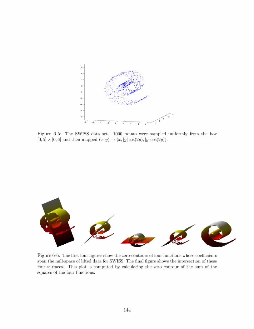
−4−2
02
4−8 −6 −4 −2 0 2 4 6 8
−8
−6
−4
−2
0
2
4
6
8
Figure 6-5: The SWISS data set. 1000 points were sampled uniformly from the box[0, 5]× [0, 6] and then mapped (x, y) 7→ (x, |y| cos(2y), |y| cos(2y)).
Figure 6-6: The first four figures show the zero-contours of four functions whose coefficientsspan the null-space of lifted data for SWISS. The final figure shows the intersection of thesefour surfaces. This plot is computed by calculating the zero contour of the sum of thesquares of the four functions.
144

Chapter 7
Conclusion
Beginning with one simple cost function, I have presented a powerful framework for
semi-supervised and unsupervised learning. The optimizations defined by this cost
function can be principally approximated using Lagrangian duality. Furthermore,
these approximations can be optimized efficiently using standard algorithms. In this
way, once we have posed a learning problem in our framework, its solution is immedi-
ate. This puts the burden on the practitioner to pose the problem, not to slave over
creating novel algorithms.
The utility of this framework was demonstrated through four very different appli-
cations. In each case, I adjoined a simple and intuitive prior to the function learning
problem and then showed how such simple additions immediately produced power-
ful algorithms. First, I considered priors on the kernel function that generates the
RKHS. From such priors, new insights into Kernel Learning were derived, and a
novel method for learning polynomial kernels was presented. Second, I showed how
the prior of binary labels lead to powerful algorithms for transductive classification
and segmentation. The segmentation algorithm generalizes the so-called spectral clus-
tering algorithms. Third, I imposed a dynamics prior on the labels and developed an
optimization that can learn a mapping between two time series. This optimization
takes as input examples of how to map individual samples of the input time series to
corresponding samples of the output time series. Because it assumes that the output
time series follows known dynamics, it can also take advantage of unlabelled input
145
samples. Finally, by applying the prior that the hidden function was constant on the
data, a new method for learning manifolds based on implicit functions was derived.
There are a variety of directions that remain to be explored. With a particu-
lar focus on the examples presented in this thesis, there are many interesting open
problems. For clustering, it would be interesting to develop methods for multiclass
classification that do not require successive application of two-way clustering algo-
rithms. It would be useful to devise a method that, when given an initial guess at
the number of clusters, K, tries to find the best K-way partitioning at once. For
the dynamics algorithms, the state transition matrices were fixed a priori. Applying
techniques from system identification [60, 71, 102], it may be possible to learn these
as well by modifying the current optimization. Furthermore, a method for semi-
supervised regression with a nonlinear dynamics model would be of great interest.
The techniques developed in Chapter 6 could be used to empirically study the con-
served quantities of dynamical systems [3, 59]. Furthermore, such methods could be
used for nonlinear system identification by finding the manifolds that are constant on
the trajectories of dynamical systems. There is an endless variety of domain specific
applications that can be derived with new output priors, and it would be interesting
to expand the toolbox of techniques that fall under this framework.
I am particularly interested in exploring further applications of the duality tools
used in Chapter 3. Recall that I was able to construct a proof of the Representer
Theorem using duality on the Hilbert Space of functions. Inspired by the polynomial
relaxation techniques that exploit positivity conditions in the dual problems [58, 73],
I hope to develop new techniques for solving quadratic problems where the primal
problem deals with very high dimensional objects. Such relaxations provide finite
dimensional convex programs that operate on sufficient statistics of the original op-
timization program. For example, in Chapter 3, I only needed to consider the inner
products of the infinite dimensional f with a finite set of vectors. It remains to be
seen if we can generalize past the results of Chapter 3 to provide further insights
into the structure of Reproducing Kernel Hilbert Spaces and devise new techniques
in machine learning.
146

There are two other areas where I believe such techniques can yield powerful new
algorithms. First, there has been substantial activity in the controls community to
develop analysis and synthesis tools for systems consisting of extremely large num-
bers of interconnected subsystems. A large part of this effort has been devoted to
developing tools that scale gracefully with the number of subsystems, and their at-
tendant local sensing, actuating, and computing elements. Clearly for systems that
are comprised of a large number of subsystems, structure must be fully exploited to
obtain tractable analysis and control synthesis algorithms.
Recent work has made a great deal of progress in exploiting the symmetry present
in such systems. Control laws can be distributed such that they only rely on lo-
cal communication, yet can still give rise to desired global behavior, and, in certain
settings, it has been shown that spatially distributed controllers are optimal for the
control of spatially invariant systems [5, 65]. The synthesis of such distributed con-
trollers is often convex [26, 104], and taking the distributed structure of a problem
into account can greatly reduce the complexity of control design without sacrificing
system performance [18].
I want to connect the recently presented techniques for the control design of spa-
tially interconnected systems [22, 23, 24] to the relaxation of duality on Hilbert spaces.
I have shown how these results are in fact applicable to a much larger class of inter-
connection topologies where the symmetry of the interconnection may be noncom-
mutative [81, 82]. The dual techniques developed in this thesis may provide further
analysis conditions which guarantee performance objectives for these interconnected
systems.
Secondly, I want to explore applications in quantum information. For a quantum
system, the Hamiltonian is the mathematical object which both governs the evolution
of the system and the energies of the various configurations. A fundamental problem
is to determine the configuration with the lowest possible energy. Such a configuration
is called the ground state of a given Hamiltonian and its corresponding energy level
is called the ground state energy [57].
The ground state energy is generally NP-HARD to calculate. Even the simple
147

looking problem of configuring an array of small quantum magnets, called spins, to
minimize their interaction energy is NP-HARD [6], although special cases can be
solved analytically [54]. Furthermore, it often requires exponentially many numbers
to describe the ground state itself. Since it is likely impossible to exactly calculate
the ground state or ground state energy of a generic quantum system, alternative
approximate means are needed to gain insight into the structure of the quantum
ground state. Many approximate techniques have been developed. Early techniques
used perturbations around a so-called “mean field” to generate useful estimates of
molecular structure [95]. The Density Matrix Renormalization Group [107] has been
widely successful in the study of chains of identical systems, but does not scale to
arbitrarily coupled topologies. Chemists in the 1950s developed analytic tools for
studying electrons [64, 66] that could only be solved in simple cases until they were
shown half a century later to be solvable by semidefinite programming [67].
I intend to study a new approach to estimating the ground state energy using
approximations of the dual problem. Noting that most Hamiltonians are presented
as sums of products of local interaction terms, redundant constraints amongst these
interactions can be adjoined to the formulation of the ground state problem. These
interactions may be easy to analyze on their own and their energy levels can be added
as redundant constraints. By relaxing the dual, I hope to produce optimization prob-
lems that are polynomial in the number of interactions. I am particularly interested
in exploring how these techniques extend the work on electrons [67] to a more widely
applicable framework and how this new approach might generalize the algorithm to
the Goemans-Williamson algorithm for MAX-CUT [37] to the quantum regime.
148

Appendix A
Linear Algebra
Many of the algebraic manipulations used in this document are based on techniques
derived from minimizing quadratic forms. Here we present some of these derivations.
A.1 Unconstrained Quadratic Programming
Given a matrix A, one can readily check that
minx
x>Ax =
0 A 0
−∞ otherwise
(A.1)
This is because if A has any negative eigenvalues, then the cost is unbounded below.
Assume A is positive semidefinite and consider the quadratic program
minx
x>Ax− 2b>x + c (A.2)
we may, differentiate with respect to x to find that at the optimum
Ax = b (A.3)
If A is invertible then the minimum is −b>A−1b + c
149

A.2 Schur Complements
Let M be a matrix partitioned as
M =
A B
B> C
(A.4)
For the simplicity of presentation, let us assume that A and B are invertible. The
Schur complement of A in M is defined to be
(M|A) = C−B>A−1B (A.5)
and the Schur complement of C in M is
(M|C) = A−BC−1B> (A.6)
A.3 More Quadratic Programming
For the quadratic minimization
minx2
x1
x2
> A B>
B C
x1
x2
− 2
b1
b2
> x1
x2
(A.7)
the optimal x∗2 is given by
x∗2 = C−1(b2 −Bx1) (A.8)
Plug that back into the cost function:
x>1 (M|C)x1 − 2(b1 −BC−1b2)>x1 (A.9)
Similarly, minimizing over x1 gives the cost function
x>2 (M|A)x2 − 2(b2 −B>A−1b1)>x2 (A.10)
150

Solving these two reduced quadratic programs gives x∗1
x∗2
=
(M|C)−1(b1 −BC−1b2)
(M|A)−1(b2 −B>A−1b2)
(A.11)
A.4 Inverting Partitioned Matrices
Since x∗1
x∗2
= M−1
b1
b2
(A.12)
we see that
M−1 =
(M|C)−1 −(M|C)−1BC−1
−(M|A)−1B>A−1 (M|A)−1
(A.13)
A.5 Schur complement Lemma
One of the most important tools used throughout the document is the Schur Com-
plement Lemma. This Lemma often allows for the transformation of polynomial
expressions into semidefinite constraints that are linear in the parameters of interest.
Lemma A.5.1 (The Schur Complement Lemma)
M 0 ⇐⇒ C 0 and (M|C) 0 (A.14)
Proof The ( =⇒ ) direction is true because subblocks of positive semidefinite ma-
trices are positive semidefinite and M−1 is positive semidefinite when M is.
To prove the reverse direction, consider minimizing (A.7) with b1 = b2 = 0. Then
for any x,
minx2
x1
x2
>M
x1
x2
= x>1 (M|C)x1 ≥ 0 (A.15)
and hence minx x>Mx ≥ 0 and M is positive semidefinite.
151

A.6 Matrix Inversion Lemma
(A−BC−1B>)−1 = A−1 + A−1B(C−B>A−1B)−1B>A−1 (A.16)
To check this, apply the partitioned matrix formula twice and set the first blocks
equal to each other.
Standard form: C → −C−1
(A + BCB>)−1 = A−1 −A−1B(C−1 + B>A−1B)−1B>A−1 (A.17)
A.7 Lemmas on Matrix Borders
Lemma A.7.1 Let A 0 be n× n and x ∈ Rn. Then
Ax =
x>Ax x>A
Ax A
0 (A.18)
Proof We will have proven the lemma if we can show that v>Axv ≥ 0 for all
v ∈ Rn+1. Partition v as [v0,v1] with v0 ∈ R and v1 ∈ Rn.
If v0 = 0, then
v>Axv = v>1 Av1 ≥ 0 (A.19)
Assume v0 6= 0. Without loss of generality, we may assume v0 = 1. Then we have
v>Axv = x>Ax + 2v>1 Ax + x>Ax =
v1
x
> A A
A A
v1
x
=
v1
x
> 1 1
1 1
⊗A
v1
x
.
(A.20)
The last expression is greater than or equal to zero for all v1 because the all ones
matrix and A are both positive semidefinite, and the tensor product of two posi-
tive semidefinite matrices is positive semidefinite. Therefore, we have shown that
v>Axv ≥ 0 as desired.
152

Lemma A.7.2 Let A 0 be n× n, x ∈ Rn, and t ∈ R. Then t x>
x A
0 (A.21)
if and only if x is in the range of A and x>A†x ≤ t.
Proof Suppose x is not in the range of A. Then x = x‖ + x⊥ with x>‖ x⊥ = 0,
x⊥ 6= 0 and x⊥ orthogonal to the range of A. Since A is hermitian, Ax⊥ = 0.
Consequently, if we set
v = − t
‖x⊥‖2x⊥ (A.22)
then we have 1
v
> t x>
x A
1
v
= t + 2v>x + v>Av
= t− 2t + 0 = −t < 0
(A.23)
violating the assumption (A.21). Similarly, if x>A†x ≥ t, the Schur Complement
Lemma tells us that (A.21) cannot hold.
The converse is an immediate consequence of A.7.1.
153

154

Appendix B
Equality Constrained Norm
Minimization on an Arbitrary
Inner Product Space
Let V be a real inner product space and let w1, . . . ,wN ∈ V , a1, . . . , aN ∈ R. Consider
the optimization
minv∈V
〈v,v〉
s.t. 〈v,wi〉 = ai for i = 1, . . . , N
(B.1)
We can construct the dual program by introducing Lagrange multipliers λi for i =
1, . . . , N and forming the Lagrangian
L(v, λ) = 〈v,v〉 − 2N∑
i=1
λi(〈v,wi〉 − ai) (B.2)
Note that, just as in the finite dimensional case, if we maximize this Lagrangian
with respect to λi, then we either get 〈v,v〉 if 〈v,wi〉 = ai for all i or ∞ otherwise.
Hence the problem (B.1) is equivalent to minv maxλ L(v, λ). The dual program is
maxλ minv L(v, λ) and always achieves a lower optimal value than the primal pro-
155
gram. We can explicitly compute the dual as follows
maxλ
minvL(v, λ) = max
λmin
v〈v,v〉 − 2
N∑i=1
λi(〈v,wi〉 − ai)
= maxλ
minv〈v,v〉 − 2〈v,
N∑i=1
λiwi〉+ 2λ>a
= maxλ
minv〈v −
N∑i=1
λiwi,v −N∑
i=1
λiwi〉
− 〈N∑
i=1
λiwi,
N∑i=1
λiwi〉+ 2λ>a
(B.3)
Since 〈u,u〉 ≥ 0 for all u ∈ V , the minimum is achieved when
v =N∑
i=1
λiwi (B.4)
This results in the dual program
maxλ−〈
N∑i=1
λiwi,N∑
i=1
λiwi〉+ 2λ>a (B.5)
If we introduce the matrix Gram matrix of the wi, W, with entries Wij = 〈wi,wj〉, we
can write this problem as an unconstrained convex quadratic program in N variables
maxλ−λ>Wλ + 2λ>a (B.6)
The set of optimal dual solutions are the solutions of the equation Wλ∗ = a. When
such a solution exists, the dual optimal value is equal to λ∗>Wλ∗, On the other hand,
when no such solution exists, the program is unbounded above. In this case, weak
duality implies that the primal program is infeasible.
When a dual optimal solution exists, consider the minimizer
v∗ = arg minvL(v, λ∗) =
N∑i=1
λ∗i wi (B.7)
156
First note that this vector is feasible for (B.1) because
〈v∗,wj〉 = 〈N∑
i=1
λ∗i wi,wj〉 =N∑
i=1
λ∗i Wij = aj (B.8)
Secondly,
〈v∗,v∗〉 = 〈N∑
i=1
λ∗i wi
N∑i=1
λ∗i wi〉 = λ∗>Wλ∗ (B.9)
That is v∗ is a primal feasible point whose primal cost is equal to the dual optimum.
This implies that v∗ is optimal for the primal and λ∗ is a geometric multiplier. Fur-
thermore, any primal optimal point v∗ is of the form∑N
i=1 λ∗i wi for some dual optimal
λ∗, all of which are geometric multipliers.
Let us summarize the preceding discussion.
Theorem B.0.3 Let V be a real inner product space and let w1, . . . ,wN ∈ V, a ∈
RN . Let W be the Gram matrix of the wj.
(i) The equality constrained norm minimization problem
minv∈V
〈v,v〉
s.t. 〈v,wi〉 = ai for i = 1, . . . , N
(B.10)
has an associated dual program
maxλ−λ>Wλ + 2λ>a (B.11)
which is an unconstrained convex quadratic program. The primal optimal value
is equal to the dual optimal value.
(ii) Suppose the optimal value of the primal-dual pair is finite. Then the set of dual
optimal solutions is given by
D := λ ∈ RN : Wλ = a (B.12)
157

and the set of primal optimal solutions is given by
P := N∑
i=1
λiwi : λ ∈ D (B.13)
158
Bibliography
[1] A. Argyriou, C. A. Micchelli, and M. Pontil. Learning convex combinations
of continuously parametrized basic kernels. In Proceedings of the 18th Annual
Conference on Learning Theory, 2005.
[2] S. Arora, S. Rao, and U. Vazirani. Expander flows, geometric embeddings, and
graph partitionings. In ACM Symposium on Theory of Computing, 2004.
[3] M. Audin. Spinning Tops. Number 51 in Cambridge studies in advanced math-
ematics. Cambridge University Press, Cambridge, UK, 1996.
[4] F. R. Bach and M. I. Jordan. Kernel independent component analysis. In
International Conference on Acoustics, Speech, and Signal Processing, 2003.
[5] B. Bamieh, F. Paganini, and M. Dahleh. Distributed control of spatially in-
variant systems. IEEE Transactions on Automatic Control, 47(7):1091–1118,
2002.
[6] F. Barahona. On the complexity of Ising spin glass models. Journal of Physics
A, 15:3241–3253, 1982.
[7] A. Beck and M. Teboulle. Mirror descent and nonlinear projected subgradient
methods for convex optimization. Operations Research Letters, 31:167–175,
2003.
[8] M. Belkin and P. Niyogi. Laplacian eigenmaps and spectral techniques for em-
bedding and clustering. In Advances in Neural Information Processing Systems,
2002.
159

[9] M. Belkin and P. Niyogi. Laplacian eigenmaps for dimensionality reduction and
data representation. Neural Computation, 15(6):1373–1396, 2003.
[10] A. Ben-Hur, D. Horn, H. T. Siegelmann, and V. Vapnik. Support vector clus-
tering. Journal of Machine Learning Research, 2:125–137, 2001.
[11] A. Ben-Tal and A. Nemirovski. Non-euclidean restricted memory level method
for large-scale convex optimization. Mathematical Programming, 102:407–456,
2005.
[12] D. P. Bertsekas, A. Nedic, and A. E. Ozdaglar. Convex Analysis and Optimiza-
tion. Athena Scientific, Belmont, MA, 2003.
[13] B. E. Boser, I. M. Guyon, and V. N. Vapnik. A training algorithm for optimal
margin classifiers. In 5th Annual ACM Workshop on COLT, pages 144–152,
1992.
[14] O. Bousquet and A. Elisseeff. Stability and generalization. Journal of Machine
Learning Research, 2(3):449–526, 2002.
[15] S. Boyd and L. Vandenberghe. Convex Optimization. Cambridge University
Press, 2003.
[16] M. Brand. Charting a manifold. In Neural Information Processing Systems
(NIPS), 2002.
[17] O. Chapelle, V. Vapnik, O. Bousquet, and S. Mukherjee. Choosing multiple
parameters for support vector machines. Machine Learning, 46(1–3):131–159,
2002.
[18] R. Cogill, S. Lall, and P. A. Parrilo. On structured semidefinite programs for
the control of symmetric systems. In Proceedings of the Allerton Conference on
Communication, Control, and Computing, 2003.
[19] F. Cucker and S. Smale. On the mathematical foundations of learning. Bulletin
of the American Mathematical Society, 39(1):1–49, 2001.
160
[20] C. L. B. D. J. Newman, S. Hettich and C. J. Merz. UCI repository of machine
learning databases, 1998.
[21] A. N. Dames. Position encoder. U.S. Patent No 5815091, September 1998.
[22] R. D’Andrea. A linear matrix inequality approach to decentralized control
of distributed parameter systems. In Proceedings of the 36th Conference on
Decision and Control, pages 1350–1354, 1997.
[23] R. D’Andrea and G. E. Dullerud. Distributed control design for spatially inter-
connected systems. IEEE Transactions on Automatic Control, 48(9):1478–1495,
2003.
[24] R. D’Andrea, C. Langbort, and R. Chandra. A state space approach to con-
trol of interconnected systems. In J. Rosenthal, editor, Mathematical Systems
Theory in Biology, Communication, Computation and Finance. Springer, IMA
Book Series, 2003. To appear.
[25] T. De Bie and N. Cristianini. Convex methods for transduction. In Neural
Information Processing Systems (NIPS), 2003.
[26] G. A. de Castro and F. Paganini. Convex synthesis of localized controllers for
spatially invariant systems. Automatica, 38:445–456, 2002.
[27] D. Donoho and C. Grimes. Hessian eigenmaps: new locally linear embedding
techniques for highdimensional data. Technical report, TR2003-08, Dept. of
Statistics, Stanford University, 2003.
[28] G. Doretto, A. Chiuso, and Y. W. S. Soatto. Dynamic textures. International
Journal of Computer Vision (IJCV), 51(2):91–109, 2003.
[29] T. Evgeniou, M. Pontil, and T. Poggio. Regularization networks and support
vector machines. Advances in Computational Mathematics, 13(1):1–50, 2000.
161

[30] U. Feige and G. Schectman. On the optimality of the random hyperplane
rounding technique for MAX-CUT. Random Structures and Algorithms, 2000.
to appear.
[31] A. Frieze and M. Jerrum. Improved approximation algorithms for MAX k-CUT
and MAX BISECTION. In E. Balas and J. Clausen, editors, Integer Program-
ming and Combinatorial Optimization, volume 920, pages 1–13. Springer, 1995.
[32] M. R. Garey and D. S. Johnson. Computers and intractability: a guide to the
theory of NP-completeness. W. H. Freeman, San Francisco, 1978.
[33] N. Gershenfeld. Sensors for real-time cello analysis and interpretation. In
Proceedings of the ICMC, 1991.
[34] Z. Ghahramani and S. Roweis. Learning nonlinear dynamical systems using
an em algorithm. In Neural Information Processing Systems (NIPS), pages
431–437, 1998.
[35] F. Girosi. An equivalence between sparse approximation and support vector
machines. Neural Computation, 10:1455–1480, 1998.
[36] K. Glashoff and S.-A. Gustafson. Linear Optimization and Approximation.
Number 45 in Applied Mathematical Sciences. Springer-Verlag, New York, 1983.
[37] M. X. Goemans and D. P. Williamson. Improved approximation algorithms
for maximum cut and satisfiability problems using semidefinite programming.
Journal of the ACM, 42:1115–1145, 1995.
[38] M. X. Goemans and D. P. Williamson. Approximation algorithms for MAX-
3-CUT and other problems via complex semidefinite programming. In ACM
Symposium on Theory of Computing, pages 443–452, 2001.
[39] M. Grotschel, L. Lovasz, and A. Schrijver. Geometric Algorithms and Combi-
natorial Optimization. Number 2 in Algorithms and Combinatorics. Springer-
Verlag, Berlin, 2nd edition, 1993.
162
[40] G. Gruber and F. Rendl. The bundle method for hard combinatorial optimiza-
tion problems. pages 78–88, 2003.
[41] V. Guilleman and A. Pollack. Differential Topology. Prentice Hall, Englewood
Cliffs, New Jersey, 1974.
[42] J. Ham, D. Lee, and L. Saul. Learning high dimensional correspondences from
low dimensional manifolds. In ICML, 2003.
[43] J. Hastad. Some optimal inapproximability results. J. ACM, 48(4):798–859,
2001.
[44] R. Hettich and K. O. Kortanek. Semi-infinite programming: Theory, methods,
and applications. SIAM Review, 35(3):380–429, 1993.
[45] R. A. Horn and C. R. Johnson. Matrix Analysis. Cambridge University Press,
New York, 1985.
[46] W.-Y. Hsiang. On infinitesimal symmetrization and volume for spherical and
hyperbolic tetrahedrons. Oxford Quarterly Journal of Mathematics, 39(2):463–
368, 1988.
[47] A. Jadbabaie, N. Motee, and M. Barahona. On the stability of the kuramoto
model of coupled nonlinear oscillators. In Proceedings of the American Control
Conference, 2004.
[48] O. Jenkins and M. Mataric. A spatio-temporal extension to isomap nonlinear di-
mension reduction. In International Conference on Machine Learning (ICML),
2004.
[49] T. Joachims. Transductive inference for text classification using support vector
machines. In International Conference on Machine Learning, pages 200–209,
1999.
163
[50] D. R. Karger, R. Motwani, and M. Sudan. Approximate graph coloring by
semidefinite programming. In IEEE Symposium on Foundations of Computer
Science, pages 2–13, 1994.
[51] H. Karloff. How good is the goemans–williamson max cut algorithm? SIAM
Journal on Computing, 29(1):336–350, 1999.
[52] H. Karloff and U. Zwick. A 7/8-approximation for MAX 3SAT. In Proceedings
of the 38th Annual IEEE Symposium on the Foundations of Computer Science,
pages 406–415, 1997.
[53] N. Karmakar. A new polynomial-time algorithm for linear programming. Com-
binatorica, 4(4):373–395, 1984.
[54] P. W. Kasteleyn. Graph theory and crystal physics. In F. Harary, editor, Graph
Theory and Theoretical Physics, pages 43–110, London, 1967. Academic Press.
[55] J. Lafferty, A. McCallum, and F. Pereira. Conditional random fields: Proba-
bilistic models for segmenting and labeling sequence data. In Proc. 18th Inter-
national Conf. on Machine Learning, pages 282–289. Morgan Kaufmann, San
Francisco, CA, 2001.
[56] G. R. G. Lanckriet, N. Cristianini, P. Bartlett, L. E. Ghaoui, and M. I. Jordan.
Learning the kernel matrix with semidefinite programming. Journal of Machine
Learning Research, 5:24–72, 2004.
[57] L. D. Landau and E. M. Lifshitz. Quantum Mechanics (Non-relativistic Theory),
volume 3 of Course of Theoretical Physics. Butterworth-Heinemann, Oxford,
3rd edition, 1977.
[58] J. B. Lasserre. Global optimization with polynomials and the problem of mo-
ments. SIAM Journal on Optimization, 11:796–817, 2001.
[59] B. Leimkuhler and S. Reich. Simulating Hamiltonian Dynamics. Cambridge
Monographs on Applied and Computational Mathematics. Cambridge Univer-
sity Press, Cambridge, UK, 2004.
164
[60] L. Ljung. System Identification. Theory for the user. Prentice Hall, Upper
Saddle River, NJ, 2nd edition, 1998.
[61] M. S. Lobo, L. Vandenberghe, S. Boyd, and H. Lebret. Applications of second-
order cone programming. Linear Algebra and its Applications, 284:193–228,
1998.
[62] M. Lopez and G. Still. Semi-infinite programming. Technical report, University
of Twente, 2005.
[63] S. H. Low, J. Doyle, and F. Paganini. Internet congestion control. IEEE Control
Systems Magazine, 2002.
[64] P.-O. Lowdin. Quantum theory of many-particle systems. i. physical interpreta-
tions by means of density matrices, natural spin-orbitals, and convergence prob-
lems in the method of configurational interaction. Physical Review, 97(6):1474–
1489, 1954.
[65] N. C. Martins, S. Venkatesh, and M. A. Dahleh. Controller design and imple-
mentation for large-scale systems, a block decoupling approach. In Proceedings
of the American Control Conference, pages 4728–4733, 2001.
[66] J. E. Mayer. Electron correlation. Physical Review, 100(6):1579–1586, 1955.
[67] D. A. Mazziotti. Variational minimization of atomic and molecular ground-
state energies via the two-particle reduced density matrix. Physical Review A,
65(6):062511–1–062511–14, 2002.
[68] Y. Nesterov. Quality of semidefinite relaxation for nonconvex quadratic opti-
mization. Technical report, CORE Discussion Paper 9719, 1997.
[69] P. Niyogi and F. Girosi. On the relationship between generalization error,
hypothesis complexity and sample complexity for radial basis functions. Neural
Computation, 8:819–842, 1996.
165

[70] P. Niyogi and F. Girosi. Generalization bounds for function approximation from
scattered noisy data. Advances in Computational Mathematics, 10:51–80, 1999.
[71] P. V. Overschee and B. D. Moor. N4sid: Subspace algorithms for the identi-
fication of combined deterministic– stochastic systems. Automatica, 30:75–93,
1994.
[72] J. A. Paradiso and N. Gershenfeld. Musical applications of electric field sensing.
Computer Music Journal, 21(2):69–89, 1997.
[73] P. Parrilo. Semidefinite programming relaxations for semialgebraic problems.
Mathematical Programming Series B, 96(2):293–320, 2003.
[74] J. Patten, H. Ishii, J. Hines, and G. Pangaro. Sensetable: a wireless object
tracking platform for tangible user interfaces. In CHI ’01: Proceedings of the
SIGCHI conference on Human factors in computing systems, pages 253–260,
New York, NY, USA, 2001. ACM Press.
[75] J. Patten, B. Recht, and H. Ishii. Audiopad: A tag-based interface for musical
performance. In New Interfaces for Musical Expression, Dublin, 2002.
[76] P. Perona and W. Freeman. A factorization approach to grouping. In European
Conference on Computer Vision (ECCV), volume 1406, pages 655–670, June
1998.
[77] A. Pinkus. N-widths in approximation theory. Springer, New York, 1985.
[78] R. Pless and I. Simon. Using thousands of images of an object. In CVPRIP,
2002.
[79] R. Post. Personal communication.
[80] A. Rahimi and B. Recht. Clustering with normalized cuts is clustering with a
hyperplane. In Statistical Learning in Computer Vision, 2004.
166

[81] B. Recht and R. D’Andrea. Exploiting symmetry for the distributed control of
spatially interconnected systems. In 42nd IEEE Conference on Decision and
Control, pages 1446–1452, 2003.
[82] B. Recht and R. D’Andrea. Distributed control of systems over discrete groups.
IEEE Transactions on Automatic Control, 49(9):1446–1452, 2004.
[83] R. Rifkin and A. Klautau. In defense of one-vs-all classification. Jorunal of
Machine Learning Reseach, 5:101–141, 2004.
[84] R. Rifkin, G. Yeo, and T. Poggio. Advances in Learning Theory: Methods,
Models and Applications, volume 190 of NATO Science Series III: Computer
and Systems Sciences, chapter Regularized Least-Squares Classification, pages
131–172. IOS Press, Amsterdam, 2003.
[85] S. Roweis and L. Saul. Nonlinear dimensionality reduction by locally linear
embedding. Science, 290(5500):2323–2326, 2000.
[86] I. J. Schoenberg. Metric spaces and positive definite functions. The Annals of
Mathematics, 44(3):522–536, 1938.
[87] B. Scholkopf, A. Smola, and K.-R. Muller. Nonlinear component analysis as a
kernel eigenvalue problem. Neural Computation, 10:1299–1319, 1998.
[88] B. Scholkopf, R. Williamson, A. Smola, J. Shawne-Taylor, and J. Platt. Sup-
port vector method for novelty detection. In Advances in Neural Information
Processing Systems 12, 2000.
[89] J. Shi and J. Malik. Normalized cuts and image segmentation. IEEE Transac-
tions on Pattern Analysis and Machine Intelligence, 22(8):888–905, 2000.
[90] J. Shi and J. Malik. Normalized cuts and image segmentation. Pattern Analysis
and Machine Intelligence (PAMI), 22(8):888–905, 2000.
[91] M. Simonovits. How to compute the volume in high dimension? Mathematical
Programming Series B, 97:337–374, 2003.
167

[92] J. R. Smith. Electric Field Imaging. PhD thesis, Massachusetts Institute of
Technology, February 1999.
[93] A. Smola, S. Mika, B. Schoelkopf, and R. C. Williamson. Regularized principal
manifolds. Journal of Machine Learning, 1:179–209, 2001.
[94] A. J. Smola, R. C. Williamson, S. Mika, and B. Scholkopf. Regularized principal
manifolds. Lecture Notes in Computer Science, 1572:214–229, 1999.
[95] A. Szabo and N. S. Ostlund. Modern Quantum Chemistry: Introduction to
Advanced Electronic Structure Theory. McGraw-Hill, New York, 1989.
[96] D. M. J. Tax and R. P. W. Duin. Support vector domain description. Pattern
Recognition Letters, 20:1191–1199, 1999.
[97] J. B. Tenenbaum, V. de Silva, and J. C. Langford. A global geometric framework
for nonlinear dimensionality reduction. Science, 290(5500):2319–2323, 2000.
[98] H. Valpola and J. Karhunen. An unsupervised ensemble learning method for
nonlinear dynamic state-space models. Neural Computation, 14(11):2647–2692,
2002.
[99] L. Vandenberghe and S. Boyd. Semidefinite programming. SIAM Review,
38(1):49–95, 1996.
[100] V. Vapnik. Statistical learning theory. Wiley, 1998.
[101] V. N. Vapnik. The nature of statistical learning theory. Springer, New York,
2nd edition, 2000.
[102] M. Verhaegen and P. Dewilde. Subspace model identification. International
Journal of Control, 56(5):1187–1210, 1992.
[103] D. Verma and M. Meila. A comparison of spectral clustering algorithms. In
http://www.cs.washington.edu/research/spectral, 2003.
168

[104] P. Voulgaris, G. Bianchini, and B. Bamieh. Optimal decentralized controllers
for spatially invariant systems. In Proceedings of the 39th IEEE Conference on
Decision and Control, pages 3763 –3768, 2000.
[105] G. Wahba. Spline Models for Observational Data. Society for Industrial and
Applied Mathematics, Philadelphia, Pennsylvania, 1990.
[106] K. Weinberger and L. Saul. Unsupervised learning of image manifolds by
semidefinite programming. In Computer Vision and Pattern Recognition
(CVPR), 2004.
[107] S. R. White. Density matrix formulation for quantum renormalization groups.
Physical Review Letters, 69(19):2863–2866, 1992.
[108] E. Xing and M. Jordan. On semidefinite relaxation for normalized k-cut and
connections to spectral clustering. Technical Report CSD-03-1265, Division of
Computer Science, University of California, Berkeley, 2003.
[109] X. Zhu, Z. Ghahramani, and J. Lafferty. Semi-supervised learning using gaus-
sian fields and harmonic functions. In ICML, 2003.
[110] T. Zimmerman, J. Smith, J. Paradiso, D. Allport, and N. Gershenfeld. Applying
electric field sensing to human-computer interfaces. In Proceedings of CHI’95:
ACM Conference on Human Factors in Computing Systems, 1995.
169