a dissertation presented in partial fulfillment of the
TRANSCRIPT

SCALING UP METRIC TEMPORAL PLANNING
by
Minh B. Do
A Dissertation Presented in Partial Fulfillmentof the Requirements for the Degree
Doctor of Philosophy
ARIZONA STATE UNIVERSITY
December 2004

ABSTRACT
This dissertation aims at building on the success of domain-independent heuristics for clas-
sical planning to develop a scalable metric temporal planner. The main contribution is Sapa, a
domain-independent heuristic forward-chaining planner which can handle various metric and tem-
poral constraints as well as multi-objective functions. Our major technical contributions include:
• The temporal planning-graph based methods for deriving heuristics that are sensitive to both
cost and makespan. We provide different approaches for propagating and tracking the goal-
achievement cost according to time and different techniques for deriving the heuristic values
guiding Sapa using these cost-functions. To improve the heuristic quality, we also present
techniques for adjusting the heuristic estimates to take into account action interactions and
metric resource limitations.
• The “partialization” techniques to convert the position-constrained plans produced by Sapa
to generate the more flexible order-constrained plans. Toward this objective, a general Con-
straint Satisfaction Optimization Problem (CSOP) is developed and can be optimized under
an objective function dealing with a variety of temporal flexibility criteria, such as makespan.
• Sapaps , an extension of Sapa, that is capable of finding solutions for the Partial Satisfaction
Planning Net Benefit (PSP Net Benefit) problems. Sapaps uses an anytime best-first search
algorithm to find plans with increasing better solution quality as it is given more time to run.
For each of these contributions, we present the technical details and demonstrate the effec-
tiveness of the implementations by comparing its performance against other state-of-the-art planners
using the benchmark planning domains.
iii

To my family.
iv

ACKNOWLEDGMENTS
First, I would like to thank my advisor Professor Subbarao Kambhampati. He is by far
my best ever advisor and tutor. His constant support in many ways (including sharp criticism),
enthusiasm, and his willingness to spend time to share his deep knowledge of various aspects of
research and life have made me never regret making one of my riskiest decision five years ago. It
feels like yesterday when I contacted him with very limited knowledge about what AI is and what
he does. However, through up and down moments, it has been an enjoyable time in Arizona, I love
what I have been doing as a student and a researcher and I am ready to take the next step, mostly
due to him.
I would specially like to acknowledge my outside committee member, Dr. David Smith of
NASA Ames for giving many insightful suggestions in a variety of my work and for taking time
from his busy schedule to participate in my dissertation. A big thanks also goes to Professor Chitta
Baral, and Professor Huan Liu for valuable advice and encouragement.
I want to thank all members of the Yochan group and the AI lab for being good supportive
friends throughout my stay. In this regard, I am particularly grateful to Biplav Srivastava, Terry
Zimmerman, XuanLong Nguyen, Romeo Sanchez, Dan Bryce, Menkes van den Briel, and J. Benton
for collaborations, comments, and critiques on my ideas and presentations. I also want to thank Tuan
Le, Nie Zaiquing, Ullas Nambiar and Sreelaksmi Valdi, William Cushing, and Nam Tran for their
companionship, their humors, and their helps when I need them most.
I am and will always be grateful to my parents for their love and for their constant belief
in me. Saving the best for last, my wife is special and has always been there understanding and
supporting me with everything I have ever needed. My son, even though you can not say more than
a few “uh ah”, I know that you meant: “I can always give you a nice smile or a good hug when you
need one”.
v

This research is supported in part by the NSF grant ABCD and the NASA grant XYZ.
vi
TABLE OF CONTENTS
Page
LIST OF TABLES . . . . . . . . . . . . . . . . . . . . . . . . . . . . . . . . . . . . . . xi
LIST OF FIGURES . . . . . . . . . . . . . . . . . . . . . . . . . . . . . . . . . . . . . xii
CHAPTER 1 Introduction . . . . . . . . . . . . . . . . . . . . . . . . . . . . . . . . . 1
CHAPTER 2 Background on Planning . . . . . . . . . . . . . . . . . . . . . . . . . . . 9
2.1. Plan Representation . . . . . . . . . . . . . . . . . . . . . . . . . . . . . . . . . . 10
2.2. Forward State-space Search Algorithm . . . . . . . . . . . . . . . . . . . . . . . . 14
2.3. Search Control and Reachability Analysis based on the Planning Graph . . . . . . 15
CHAPTER 3 Handling concurrent actions in a forward state space planner . . . . . . . . 21
3.1. Action Representation and Constraints . . . . . . . . . . . . . . . . . . . . . . . . 21
3.2. A Forward Chaining Search Algorithm for Metric Temporal Planning . . . . . . . 25
3.3. Summary and Discussion . . . . . . . . . . . . . . . . . . . . . . . . . . . . . . . 30
CHAPTER 4 Heuristics based on Propagated Cost-Functions over the Relaxed Planning
Graph . . . . . . . . . . . . . . . . . . . . . . . . . . . . . . . . . . . . . . . . . . 32
4.1. The Temporal Planning Graph Structure . . . . . . . . . . . . . . . . . . . . . . . 34
4.2. Cost Propagation Procedure . . . . . . . . . . . . . . . . . . . . . . . . . . . . . 35
4.3. Termination Criteria for the Cost Propagation Process . . . . . . . . . . . . . . . . 40
4.4. Heuristics based on Propagated Cost Functions . . . . . . . . . . . . . . . . . . . 43
4.4.1. Directly Using Cost Functions to Estimate C(PS): . . . . . . . . . . . . . 45
4.4.2. Computing Cost from the Relaxed Plan: . . . . . . . . . . . . . . . . . . . 46
vii
Page
4.4.3. Origin of Action Costs: . . . . . . . . . . . . . . . . . . . . . . . . . . . . 49
4.5. Adjustments to the Relaxed Plan Heuristic . . . . . . . . . . . . . . . . . . . . . . 50
4.5.1. Improving the Relaxed Plan Heuristic Estimation with Static Mutex Relations 50
4.5.2. Using Resource Information to Adjust the Cost Estimates . . . . . . . . . 52
4.6. Summary and Discussion . . . . . . . . . . . . . . . . . . . . . . . . . . . . . . . 54
CHAPTER 5 Implementation & Empirical Evaluation . . . . . . . . . . . . . . . . . . . 58
5.1. Component Evaluation . . . . . . . . . . . . . . . . . . . . . . . . . . . . . . . . 60
5.2. Sapa in the 2002 International Planning Competition . . . . . . . . . . . . . . . . 64
CHAPTER 6 Improving Solution Quality by Partialization . . . . . . . . . . . . . . . . 73
6.1. Problem Definition . . . . . . . . . . . . . . . . . . . . . . . . . . . . . . . . . . 74
6.2. Formulating a CSOP encoding for the Partialization Problem . . . . . . . . . . . . 76
6.3. Greedy Approach for Solving the partialization encoding . . . . . . . . . . . . . . 83
6.4. Solving the CSOP Encoding by Converting it to MILP Encoding . . . . . . . . . . 85
6.5. Partialization: Implementation . . . . . . . . . . . . . . . . . . . . . . . . . . . . 91
6.5.1. Greedy Partialization Approach . . . . . . . . . . . . . . . . . . . . . . . 92
6.5.2. Use of Greedy Partialization at IPC-2002 . . . . . . . . . . . . . . . . . . 94
6.5.3. Optimal Makespan Partialization . . . . . . . . . . . . . . . . . . . . . . . 97
6.6. Summary and Discussion . . . . . . . . . . . . . . . . . . . . . . . . . . . . . . . 100
CHAPTER 7 Adapting Best-First Search to Partial-Satisfaction Planning . . . . . . . . . 102
7.1. Anytime Search Algorithm for PSP Net Benefit . . . . . . . . . . . . . . . . . . . 107
7.2. Heuristic for Sapaps . . . . . . . . . . . . . . . . . . . . . . . . . . . . . . . . . 113
viii
Page
7.3. Sapaps : Implementation . . . . . . . . . . . . . . . . . . . . . . . . . . . . . . . 116
7.4. Summary and Discussion . . . . . . . . . . . . . . . . . . . . . . . . . . . . . . . 119
CHAPTER 8 Related Work and Discussion . . . . . . . . . . . . . . . . . . . . . . . . 122
8.1. Metric Temporal Planning . . . . . . . . . . . . . . . . . . . . . . . . . . . . . . 122
8.2. Partialization . . . . . . . . . . . . . . . . . . . . . . . . . . . . . . . . . . . . . 127
8.3. Partial Satisfaction (Over-Subscription) Problem . . . . . . . . . . . . . . . . . . 130
CHAPTER 9 Conclusion and Future Work . . . . . . . . . . . . . . . . . . . . . . . . . 134
9.1. Summary . . . . . . . . . . . . . . . . . . . . . . . . . . . . . . . . . . . . . . . 134
9.2. Future Work . . . . . . . . . . . . . . . . . . . . . . . . . . . . . . . . . . . . . . 135
REFERENCES . . . . . . . . . . . . . . . . . . . . . . . . . . . . . . . . . . . . . . . 137
APPENDIX A PLANNING DOMAIN AND PROBLEM REPRESENTATION . . . . . . 148
A.1. STRIPS Representation in PDDL1.0 Planning Language . . . . . . . . . . . . . . 149
A.1.1. Domain Specification: Satellite . . . . . . . . . . . . . . . . . . . . . . . 149
A.1.2. Problem Specification: Satellite . . . . . . . . . . . . . . . . . . . . . . . 151
A.2. Metric Temporal Planning with PDDL2.1 Planning Language . . . . . . . . . . . . 153
A.2.1. Domain Specification: Satellite . . . . . . . . . . . . . . . . . . . . . . . 153
A.2.2. Problem Specification: Satellite . . . . . . . . . . . . . . . . . . . . . . . 156
A.3. Extending PDDL2.1 for PSP Net Benefit . . . . . . . . . . . . . . . . . . . . . . . 162
A.3.1. Domain Specification: ZenoTravel . . . . . . . . . . . . . . . . . . . . . . 162
A.3.2. Problem Specification: ZenoTravel . . . . . . . . . . . . . . . . . . . . . . 165
A.3.3. Domain Specification: Satellite . . . . . . . . . . . . . . . . . . . . . . . 168
ix
Page
A.3.4. Problem Specification: Satellite . . . . . . . . . . . . . . . . . . . . . . . 172
APPENDIX B CSOP AND MILP ENCODING . . . . . . . . . . . . . . . . . . . . . . 178
B.1. CSOP Encoding for Partialization . . . . . . . . . . . . . . . . . . . . . . . . . . 179
B.2. MILP Encoding . . . . . . . . . . . . . . . . . . . . . . . . . . . . . . . . . . . . 180
x

LIST OF TABLES
Table Page
1. Compare different makespan values in the IPC’s domains . . . . . . . . . . . . . . 95
2. Compare optimal and greedy partializations . . . . . . . . . . . . . . . . . . . . . 98
xi
LIST OF FIGURES
Figure Page
1. Architecture of Sapa . . . . . . . . . . . . . . . . . . . . . . . . . . . . . . . . . 3
2. Planning and its branches [48]. . . . . . . . . . . . . . . . . . . . . . . . . . . . . 10
3. Example of plan in STRIPS representation. . . . . . . . . . . . . . . . . . . . . . 11
4. Example of the Planning Graph. . . . . . . . . . . . . . . . . . . . . . . . . . . . 17
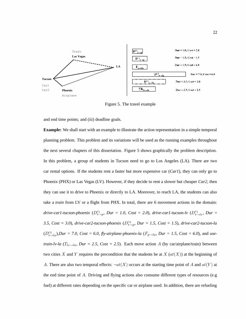
5. The travel example . . . . . . . . . . . . . . . . . . . . . . . . . . . . . . . . . . 22
6. Sample Drive-Car action in PDDL2.1 Level 3 . . . . . . . . . . . . . . . . . . . . 24
7. Main search algorithm . . . . . . . . . . . . . . . . . . . . . . . . . . . . . . . . 29
8. An example showing how different datastructures representing the search state
S = (P,M,Π, Q) change as we advance the time stamp, apply actions and acti-
vate events. The top row shows the initial state. The second row shows the events
and actions that are activated and executed at each given time point. The lower rows
show how the search state S = (P,M,Π, Q) changes due to action application.
Finally, we show graphically the durative actions in this plan. . . . . . . . . . . . . 30
9. Main cost propagation algorithm . . . . . . . . . . . . . . . . . . . . . . . . . . . 36
10. Timeline to represent actions at their earliest possible execution times in the relaxed
temporal planning graph. . . . . . . . . . . . . . . . . . . . . . . . . . . . . . . . 38
11. Cost functions for facts and actions in the travel example. . . . . . . . . . . . . . . 39
12. Procedure to extract the relaxed plan . . . . . . . . . . . . . . . . . . . . . . . . . 46
13. Example of mutex in the relaxed plan . . . . . . . . . . . . . . . . . . . . . . . . 51
14. Screen shot of Sapa’s GUI: PERT chart showing the actions’ starting times and the
precedence orderings between them. . . . . . . . . . . . . . . . . . . . . . . . . . 59
xii
Figure Page
15. Screen shots of Sapa’s GUI: Gant chart showing different logical relations between
a given action and other actions in the plan. . . . . . . . . . . . . . . . . . . . . . 60
16. Cost and makespan variations according to different weights given to them in the
objective function. Each point in the graph corresponds to an average value over 20
problems. . . . . . . . . . . . . . . . . . . . . . . . . . . . . . . . . . . . . . . . 61
17. Comparison of the different lookahead options in the competition domains. These
experiments were run on a Pentium III-750 WindowsXP machine with 256MB of
RAM. The time cutoff is 600 seconds. . . . . . . . . . . . . . . . . . . . . . . . . 69
18. Utility of the resource adjustment technique on ZenoTravel (time setting) domain
in the competition. Experiments were run on a WindowsXP Pentium III 750MHz
with 256MB of RAM. Time cutoff is 600 seconds. . . . . . . . . . . . . . . . . . 70
19. Results for the time setting of the Satellite domain (from IPC3 results). . . . . . . . 70
20. Results for the complex setting of the Satellite domain (from IPC3 results). . . . . . 70
21. Results for the time setting of the Rover domain (from IPC3 results). . . . . . . . . 71
22. Results for the time setting of the Depots domain (from IPC3 results). . . . . . . . 71
23. Results for the time setting of the DriverLog domain (from IPC3 results). . . . . . 71
24. Results for the time setting of the ZenoTravel domain (from IPC3 results). . . . . . 72
25. Examples of p.c. and o.c. plans . . . . . . . . . . . . . . . . . . . . . . . . . . . 74
26. Example of plans with different action orderings. . . . . . . . . . . . . . . . . . . 90
27. Compare different makespan values for random generated temporal logistics problems 93
28. Comparing the quality (in terms of makespan) of the plan returned by Sapa to MIPS
and TP4 in “Satellite” and “Rover” domains–two of the most expressive domains
motivated by NASA applications. . . . . . . . . . . . . . . . . . . . . . . . . . . 94
xiii
Figure Page
29. Compare different makespan values for problems in ZenoSimpletime and ZenoTime
domains . . . . . . . . . . . . . . . . . . . . . . . . . . . . . . . . . . . . . . . . 96
30. Compare different makespan values for problems in DriverlogSimpletime and
DriverlogTime domains . . . . . . . . . . . . . . . . . . . . . . . . . . . . . . . . 96
31. Compare different makespan values for problems in SatelliteTime and Satellite-
Complex domains . . . . . . . . . . . . . . . . . . . . . . . . . . . . . . . . . . . 97
32. Compare different makespan values for problems in RoversSimpletime and Rover-
sTime domains . . . . . . . . . . . . . . . . . . . . . . . . . . . . . . . . . . . . 97
33. The travel example . . . . . . . . . . . . . . . . . . . . . . . . . . . . . . . . . . 103
34. Sample Travel action in the extended PDDL2.1 Level 3 with cost field. . . . . . . . 104
35. Anytime A* search algorithm for PSP problems. . . . . . . . . . . . . . . . . . . 110
36. Cost function of goal At(DL) . . . . . . . . . . . . . . . . . . . . . . . . . . . . 112
37. A relaxed plan and goals supported by each action. . . . . . . . . . . . . . . . . . 114
38. Action costs in the extended PDDL2.1 Level 3 with cost field. . . . . . . . . . . . 115
39. Comparing Sapaps against greedy search in the ZenoTravel . . . . . . . . . . . . . 117
40. . . . . . . . . . . . . . . . . . . . . . . . . . . . . . . . . . . . . . . . . . . . . 179
xiv
CHAPTER 1
Introduction
Many real-world planning problems in manufacturing, logistics, and space applications in-
volve metric and temporal constraints. Until recently, most of the planners that were used to tackle
those problems such as HSTS/RAX [68], ASPEN [14], O-Plan [15] all relied on the availability
of domain and planner-dependent control knowledge, the collection and maintenance of which is
admittedly a laborious and error-prone activity. An obvious question is whether it will be possible
to develop domain-independent metric temporal planners that are capable of scaling up to such do-
mains. The past experience has not been particularly encouraging. Although there have been some
ambitious attempts–including IxTeT [37] and Zeno [75], their performance has not been particularly
satisfactory without an extensive set of additional control rules.
Some encouraging signs however are the recent successes of domain-independent heuristic
planning techniques in classical planning [70, 7, 41]. Our research is aimed at building on these
successes to develop a scalable metric temporal planner. At first blush search control for metric
temporal planners would seem to be a very simple matter of adapting the work on heuristic planners
in classical planning [7, 70, 41]. The adaptation however does pose several challenges:
• Metric temporal planners tend to have significantly larger search spaces than classical plan-
ners. After all, the problem of planning in the presence of durative actions and metric re-
2
sources subsumes both classical planning and a certain class of scheduling problems.
• Compared to classical planners, which only have to handle the logical constraints between
actions, metric temporal planners have to deal with many additional types of constraints that
involve time and continuous functions representing different types of resources.
• In contrast to classical planning, where the only objective is to find shortest length plans,
metric temporal planning is multi-objective. The user may be interested in improving either
temporal quality of the plan (e.g. makespan) or its cost (e.g. cumulative action cost, cost of
resources consumed etc.), or more generally, a combination thereof. Consequently, effective
plan synthesis requires heuristics that are able to track both these aspects in an evolving plan.
Things are further complicated by the fact that these aspects are often inter-dependent. For
example, it is often possible to find a “cheaper” plan for achieving goals, if we are allowed
more time to achieve them.
This dissertation presents Sapa, a heuristic metric temporal planner that we developed to
address these challenges. Sapa is a forward chaining planner, which searches in the space of
time-stamped states. Sapa handles durative actions as well as actions consuming continuous re-
sources. Our main focus has been on the development of heuristics for focusing Sapa’s multi-
objective search. These heuristics are derived from the optimistic reachability information encoded
in the planning graph. Unlike classical planning heuristics (c.f,[70]), which need only estimate the
“length” of the plan needed to achieve a set of goals, Sapa’s heuristics need to be sensitive to both
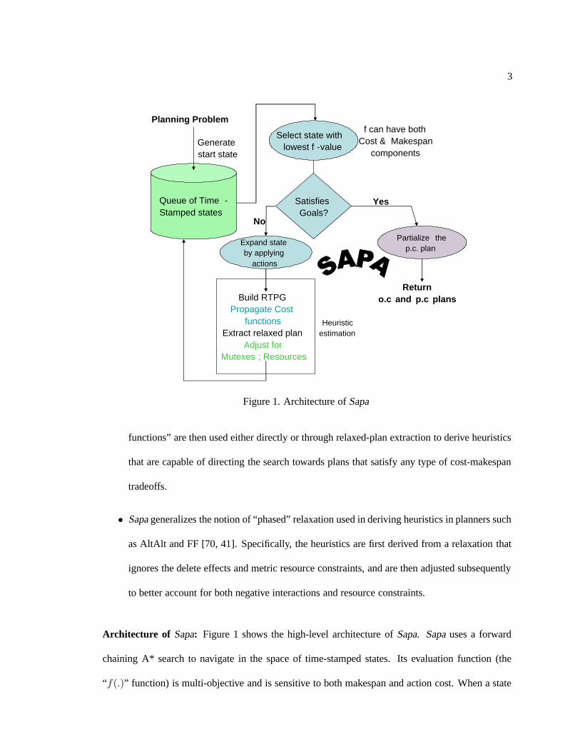
the cost and length (“makespan”) of the plans. Our contributions include:
• We present a novel framework for tracking the cost of literals (goals) as a function of time.
We present several different ways to propagate costs and terminate this tracking process, each
gives different tradeoff between the heuristic quality and the propagation time. These “cost
3
Build RTPG Propagate Cost
functions Extract relaxed plan
Adjust for Mutexes ; Resources
Planning Problem
Generate start state
No
Partialize the p.c. plan
Return o.c and p.c plans
Expand state by applying
actions
Heuristic estimation
Select state with lowest f - value
Satisfies Goals?
Queue of Time - Stamped states
Yes
f can have both Cost & Makespan
components
Figure 1. Architecture of Sapa
functions” are then used either directly or through relaxed-plan extraction to derive heuristics
that are capable of directing the search towards plans that satisfy any type of cost-makespan
tradeoffs.
• Sapa generalizes the notion of “phased” relaxation used in deriving heuristics in planners such
as AltAlt and FF [70, 41]. Specifically, the heuristics are first derived from a relaxation that
ignores the delete effects and metric resource constraints, and are then adjusted subsequently
to better account for both negative interactions and resource constraints.
Architecture of Sapa: Figure 1 shows the high-level architecture of Sapa. Sapa uses a forward
chaining A* search to navigate in the space of time-stamped states. Its evaluation function (the
“f(.)” function) is multi-objective and is sensitive to both makespan and action cost. When a state
4
is picked from the search queue and expanded, Sapa computes heuristic estimates of each of the
resulting child states. The heuristic estimation of a state S is based on (i) computing a relaxed
temporal planning graph (RTPG) from S, (ii) propagating cost of achievement of literals in the
RTPG with the help of time-sensitive cost functions (iii) extracting a relaxed plan P r for supporting
the goals of the problem and (iv) modifying the structure of P r to adjust for mutex and resource-
based interactions. Finally, P r is used as the basis for deriving the heuristic estimate of S. The
search ends when a state S ′ selected for expansion satisfies the goals. After a plan is found, we have
an option to post-process the “position constrained” plan corresponding to the state S by converting
it into a more flexible “order constrained” plan. This last step, which is the focus of the second
part of this dissertation, is done to improve the makespan as well as the execution flexibility of the
solution plan.
A version of Sapa using a subset of the techniques discussed in this paper performed well
in domains with metric and temporal constraints in the third International Planning Competition,
held at AIPS 2002 [27]. In fact, it is the best planner in terms of solution quality and number of
problems solved in the highest level of PDDL2.1 used in the competition for the domains Satellite
and Rovers (both are inspired by NASA applications.)
While the main part of the dissertation concentrates on the search algorithm and heuristic
estimate used in Sapa to solve the metric temporal planning problems, we also investigate several
important extensions to the basic algorithm in Sapa. They are: (i) the partialization algorithm that
can be used as a post-processor in Sapa to convert its position-constrained plans into the more flex-
ible order-constrained plans; and (ii) extending Sapa to solve the more general Partial Satisfaction
Planning (PSP) Net Benefit planning problems where goals can be “soft” and have different utility
values.
Improving Sapa Solution Quality: Plans for metric temporal domains can be classified broadly

5
into two categories–“position constrained” (p.c.) and “order constrained” (o.c.). The former speci-
fies the exact start time for each of the actions in the plan, while the latter only specifies the relative
orderings between the actions. The two types of plans offer complementary tradeoffs vis a vis search
and execution. Specifically, constraining the positions gives complete state information about the
partial plan, making it easier to control the search. Not surprisingly, several of the more effec-
tive methods for plan synthesis in metric temporal domains search for and generate p.c. plans (c.f.
TLPlan[1], Sapa[19], TGP [81], MIPS[24]). At the same time, from an execution point of view, o.c.
plans are more advantageous than p.c. plans –they provide better execution flexibility both in terms
of makespan and in terms of “scheduling flexibility” (which measures the possible execution traces
supported by the plan [87, 71]). They are also more effective in interfacing the planner to other
modules such as schedulers (c.f. [86, 59]), and in supporting replanning and plan reuse [90, 45].
A solution to the dilemma presented by these complementary tradeoffs is to search in the
space of p.c. plans, then post-process the resulting p.c. plan into an o.c. plan. Although such
post-processing approaches have been considered in classical planning ([49, 90, 2]), the problem is
considerably more complex in the case of metric temporal planning. The complications include the
need to handle (i) the more expressive action representation and (ii) a variety of objective functions
for partialization (in the case of classical planning, we just consider the least number of orderings)
Regarding the conversion problem discussed above, our contribution in this dissertation is to
first develop a Constraint Satisfaction Optimization Problem (CSOP) encoding for converting a p.c.
plan in metric/temporal domains produced by Sapa into an o.c. plan. This general framework allows
us to specify a variety of objective functions to choose between the potential partializations of the
p.c. plan. Among several approaches to solve this CSOP encoding, we will discuss in detail the one
approach that converts it into an equivalent Mixed Integer Linear Programming (MILP) encoding,
which can then be solved using any MILP solver such as CPLEX or LPSolve to produce an o.c. plan
6
optimized for some objective function. Besides our intention of setting up this encoding to solve
it to optimum (which is provably NP-hard [2]), we also want to use it for baseline characterization
of the “greedy” partialization algorithms. The greedy algorithms that we present can themselves
be seen as specific variable and value ordering strategies over the CSOP encoding. Our results
show that the temporal flexibility measures, such as the makespan, of the plans produced by Sapa
can be significantly improved while retaining its efficiency advantages. The greedy partialization
algorithms were used as part of the Sapa implementation that took part in the 2002 International
Planning Competition [27] and helped improve the quality of the plans produced by Sapa. We also
show that at least for the competition domains, the option of solving the encodings to optimum,
besides being significantly more expensive, is not particularly effective in improving the makespan
further.
Extending Sapa to handle PSP Net Benefit problems: Many metric temporal planning problems
can be characterized as over-subscription problems (c.f. [84, 85]) in that goals have different values
and the planning system must choose a subset that can be achieved within the time and resource
limits. Examples of the over-subscription problems include many of NASA planning problems
such as planning for telescopes like Hubble[56], SIRTF[57], Landsat 7 Satellite[78]; and planning
science for Mars rover [84]. Given the resource and time limits, only certain set of goals can be
achieved and thus it’s best to achieve the subset of goals that have highest total value given those
constraints. In this dissertation, we consider a subclass of the over-subscription problem where
goals have different utilities (or values) and actions incur different execution costs. The objective is
to find the most beneficial plan, that is the plan with the best tradeoff between the total benefit of
achieved goals and the total execution cost of actions in the plan. We refer to this subclass of the
over-subscription problem as Partial-Satisfaction Planning (PSP) Net Benefit problem where not all
the goals need to be satisfied by the final plan.

7
Current planning systems are not designed to solve the over-subscription or PSP problems.
Most of them expect a set of conjunctive goals of equal value and the planning process does not
terminate until all the goals are achieved. Extending the traditional planning techniques to solve the
over-subscription problem poses several challenges:
• The termination criteria for the planning process change because there is no fixed set of con-
juntive goals to satisfy.
• Heuristic guidance in the traditional planning systems are designed to guide the planners to
achieve a fixed set of goals. They can not be used directly in the over-subscription problem.
• Plan quality should take into account not only action costs but also the values of goals
achieved by the final plan.
In this dissertation, we discuss a new heuristic framework based on A* search for solving
the PSP problem by treating the top-level goals as soft-constraints. The search framework does not
concentrate on achieving a particular subset of goals, but rather decides the best solution for each
node in a search tree. The evaluations of the g and h values of nodes in the A* search tree are based
on the subset of goals achieved in the current search node and the best potential beneficial plan from
the current state to achieve a subset of the remaining goals. We implement this technique over the
Sapa planner and show that the resulting Sapaps planner can produce high quality plans compared
to the greedy approach.
Organization: We start with Chapter 2 on the background on relevant planning issues. Then, in
Chapter 3, we discuss the metric temporal planning representation and forward search algorithm
used in Sapa. Next, in Chapter 4, we address the problem of (i) propagating the time and cost
information over a temporal planning graph; and (ii) how the propagated information can be used to
estimate the cost of achieving the goals from a given state. We also discuss in that chapter how the
8
mutual exclusion relations and resource information help improve the heuristic estimate. Chapter 5
shows empirical results where Sapa produces plans with tradeoffs between cost and makespan, and
analyze its performance in the 2002 International Planning Competition (IPC 2002).
To improve the quality of the solution, Chapter 6 discusses the problem of converting the
“position-constrained” plans produced by Sapa to more flexible “order-constrained” plans. In this
chapter, the problem definition is given in Section 6.1, the overall Constraint Satisfaction Optimiza-
tion Problem (CSOP) encoding that captures the partialization problem is described in Section 6.2.
Next, for solving this problem, in Section 6.3 and Section 6.4, we discuss the linear-time greedy
and MILP-based optimal approaches for solving this CSOP encoding.
The next chapter of the dissertation (Chapter 7) discusses the extensions of Sapa to handle
the Partial-Satisfaction Net Benefit Planning (PSP Net Benefit) problem. This chapter contains Sec-
tion 7.1 on extending the search framework in Sapa to build the anytime heuristic search in Sapaps ;
and Section 7.2 the heuristic estimation for PSP Net Benefit problems. We also present some prelim-
inary empirical results comparing Sapaps with other search frameworks in Section 7.3. Chapter 8
contains sections on the related work, and Chapter 9 concludes the dissertation and provide the
future work that we plan to pursue.
CHAPTER 2
Background on Planning
Intelligent agency involves controlling the evolution of external environments in desirable
ways. Planning provides a way in which the agent can maximize its chances of effecting this control.
Informally, a plan can be seen as a course of actions that the agent decides upon based on its overall
goals, information about the current state of the environment, and the dynamic of its evolution.
The complexity of plan synthesis depends on a variety of properties of the environment and the
agent. Perhaps the simplest case of planning occurs when: (i) the environment is static (i.e. in
that it changes only in response to the agent’s action); (ii) observable (i.e. the agent has a complete
knowledge of the world at all times); (iii) the agent’s actions have deterministic effects on the state of
the environment; (iv) actions are instantaneous (no temporal constraint involvement); and (v) world
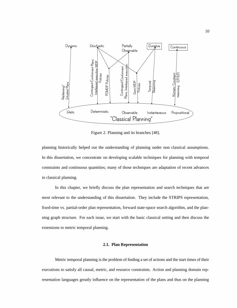
states and action’s preconditions and effects only involve boolean state variables. Figure 2 shows
this simplest case of planning (aka “classical” planning) and other branches that diverge from the
above simplest assumptions. For example, conformant and contingent planning deal with scenarios
where the environment is partially-observable, and temporal planning concentrates on problems
where durative actions and other types of temporal constraints are necessary. Despite its limitation
and the fact that most real-world applications require one or more planning properties beyond the
classical specifications (e.g. non-deterministic or durative actions), classical planning problems are
still computationally hard, and have received a significant amount of attention. Work in classical
10
Static Deterministic Observable Instantaneous Propositional
“Classical Planning”
Dynamic
Repl
a nni
ng/
Situ
a ted
Plan
s
Durative
Tem
pora
lRe
ason
ing
Continuous
Num
eric
Con
stra
int
reas
onin
g(L
P/ILP
)
Stochastic
Con
tinge
nt/C
onfo
rman
t Pla n
s,In
terle
aved
exec
utio
nM
DP
Polic
ies
POM
DP
Polic
ies
PartiallyObservable
Con
tinge
nt/C
onfo
rman
tPl
ans,
Inte
r leav
edex
ecut
ion
Sem
i-MD
PPo
licie
s
Figure 2. Planning and its branches [48].
planning historically helped out the understanding of planning under non classical assumptions.
In this dissertation, we concentrate on developing scalable techniques for planning with temporal
constraints and continuous quantities; many of those techniques are adaptation of recent advances
in classical planning.
In this chapter, we briefly discuss the plan representation and search techniques that are
most relevant to the understanding of this dissertation. They include the STRIPS representation,
fixed-time vs. partial-order plan representation, forward state-space search algorithm, and the plan-
ning graph structure. For each issue, we start with the basic classical setting and then discuss the
extensions to metric temporal planning.
2.1. Plan Representation
Metric temporal planning is the problem of finding a set of actions and the start times of their
executions to satisfy all causal, metric, and resource constraints. Action and planning domain rep-
resentation languages greatly influence on the representation of the plans and thus on the planning
11
Actions:
A1
p
q
r
¬q
A2r
s
g
PDDL: (action A1
:preconditions
(and p q)
:effects:
(and r (not q))
)
The Plan
Initial State
{p,q,s,¬r,¬g} A1 A2
Goal State
{g}
p
q
s
A1A2
rg
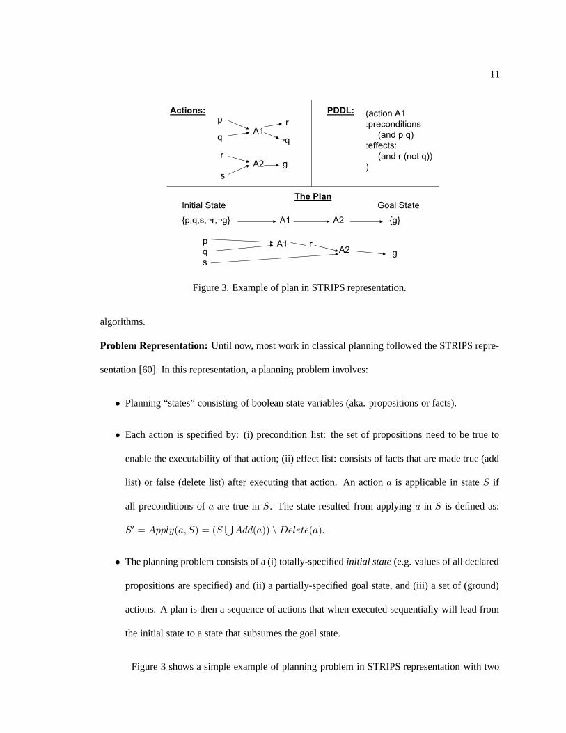
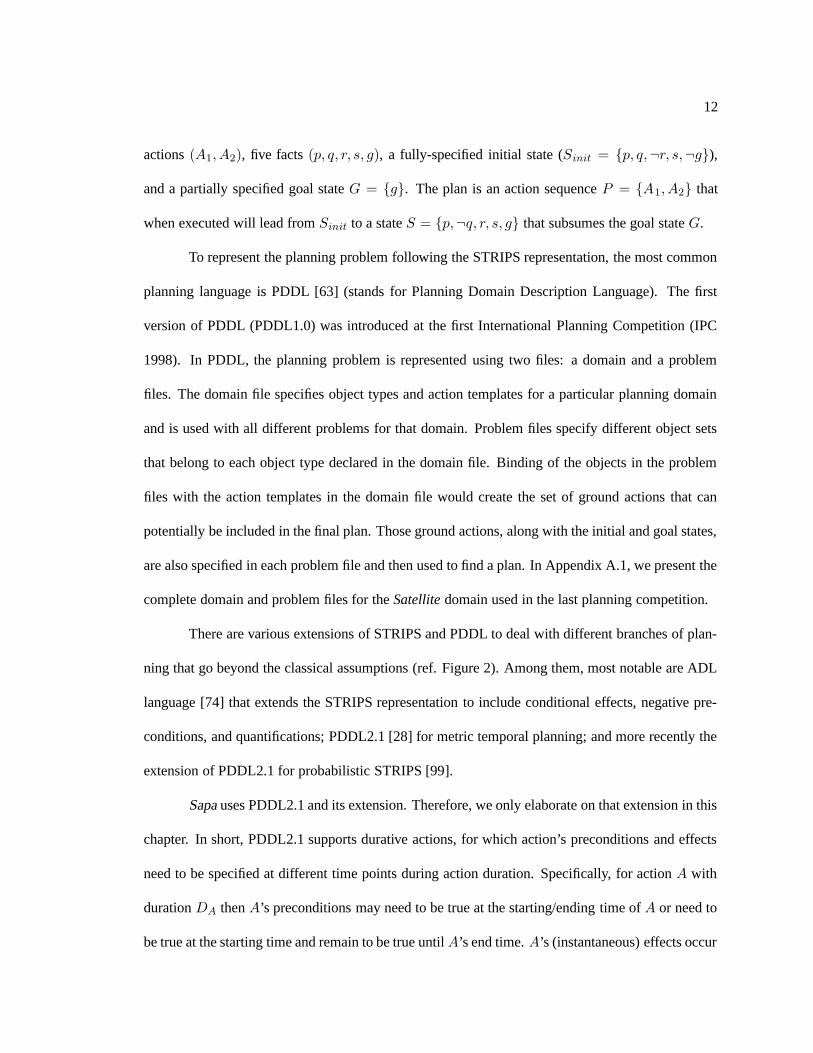
Figure 3. Example of plan in STRIPS representation.
algorithms.
Problem Representation: Until now, most work in classical planning followed the STRIPS repre-
sentation [60]. In this representation, a planning problem involves:
• Planning “states” consisting of boolean state variables (aka. propositions or facts).
• Each action is specified by: (i) precondition list: the set of propositions need to be true to
enable the executability of that action; (ii) effect list: consists of facts that are made true (add
list) or false (delete list) after executing that action. An action a is applicable in state S if
all preconditions of a are true in S. The state resulted from applying a in S is defined as:
S′ = Apply(a, S) = (S⋃
Add(a)) \Delete(a).
• The planning problem consists of a (i) totally-specified initial state (e.g. values of all declared
propositions are specified) and (ii) a partially-specified goal state, and (iii) a set of (ground)
actions. A plan is then a sequence of actions that when executed sequentially will lead from
the initial state to a state that subsumes the goal state.
Figure 3 shows a simple example of planning problem in STRIPS representation with two
12
actions (A1, A2), five facts (p, q, r, s, g), a fully-specified initial state (Sinit = {p, q,¬r, s,¬g}),
and a partially specified goal state G = {g}. The plan is an action sequence P = {A1, A2} that
when executed will lead from Sinit to a state S = {p,¬q, r, s, g} that subsumes the goal state G.
To represent the planning problem following the STRIPS representation, the most common
planning language is PDDL [63] (stands for Planning Domain Description Language). The first
version of PDDL (PDDL1.0) was introduced at the first International Planning Competition (IPC
1998). In PDDL, the planning problem is represented using two files: a domain and a problem
files. The domain file specifies object types and action templates for a particular planning domain
and is used with all different problems for that domain. Problem files specify different object sets
that belong to each object type declared in the domain file. Binding of the objects in the problem
files with the action templates in the domain file would create the set of ground actions that can
potentially be included in the final plan. Those ground actions, along with the initial and goal states,
are also specified in each problem file and then used to find a plan. In Appendix A.1, we present the
complete domain and problem files for the Satellite domain used in the last planning competition.
There are various extensions of STRIPS and PDDL to deal with different branches of plan-
ning that go beyond the classical assumptions (ref. Figure 2). Among them, most notable are ADL
language [74] that extends the STRIPS representation to include conditional effects, negative pre-
conditions, and quantifications; PDDL2.1 [28] for metric temporal planning; and more recently the
extension of PDDL2.1 for probabilistic STRIPS [99].
Sapa uses PDDL2.1 and its extension. Therefore, we only elaborate on that extension in this
chapter. In short, PDDL2.1 supports durative actions, for which action’s preconditions and effects
need to be specified at different time points during action duration. Specifically, for action A with
duration DA then A’s preconditions may need to be true at the starting/ending time of A or need to
be true at the starting time and remain to be true until A’s end time. A’s (instantaneous) effects occur
13
at either its start or end time points. While PDDL2.1 has limitations, and there are proposed more
expressive language such as PDDL+ [29] to enable the representation of more types of temporal
and continuous metric constraints, PDDL2.1 is still a language of choice for most current domain-
independent temporal planning systems. We elaborate on the description of this language with an
example in the next chapter (Chapter 3) (along with the search algorithm employed by Sapa for
searching for plan using this language.) We also present examples showing the full domain and
problem description in the Satellite domain in the Appendix A.2.
Plan Representation: For the STRIPS representation, depending on the problem specification and
the involving constraints, there are many ways to represent a plan. While the most common ap-
proach is to represent plans as sequences of actions with fixed starting times, a plan can also be
represented as a set of actions and the ordering relations between them (aka. order-constrained or
partial order causal link - POCL plans), as a tree or graph with branching points for contingency
plan, a hierarchical task network (HTN), or a “policy” that maps each possible state to a particu-
lar action. Nevertheless, for classical and metric temporal planning, the most common format are
actions with fixed starting time or order-constrained plans.
Using the first approach, each action in the final plan is associated with a starting time point.
For classical planning where there is no notion of time, we can use “level” to represent the position
of an action in the plan. The orderings between every pair of actions in the plan are totally specified
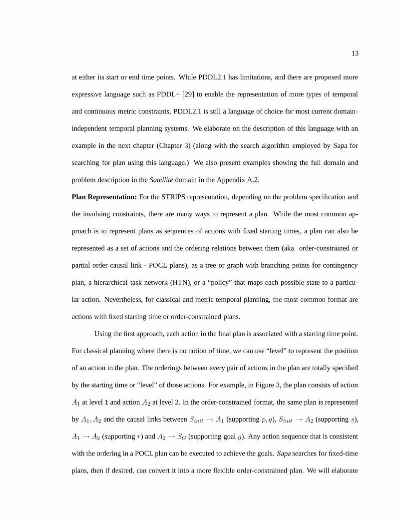
by the starting time or “level” of those actions. For example, in Figure 3, the plan consists of action
A1 at level 1 and action A2 at level 2. In the order-constrained format, the same plan is represented
by A1, A2 and the causal links between Sinit → A1 (supporting p, q), Sinit → A2 (supporting s),
A1 → A2 (supporting r) and A2 → SG (supporting goal g). Any action sequence that is consistent
with the ordering in a POCL plan can be executed to achieve the goals. Sapa searches for fixed-time
plans, then if desired, can convert it into a more flexible order-constrained plan. We will elaborate
14
more on the temporal order-constrained plan and the conversion technique in Chapter 6.
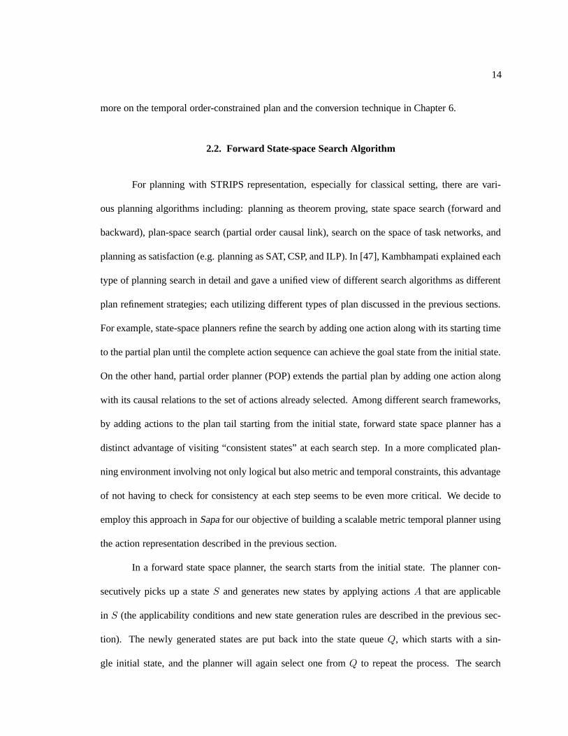
2.2. Forward State-space Search Algorithm
For planning with STRIPS representation, especially for classical setting, there are vari-
ous planning algorithms including: planning as theorem proving, state space search (forward and
backward), plan-space search (partial order causal link), search on the space of task networks, and
planning as satisfaction (e.g. planning as SAT, CSP, and ILP). In [47], Kambhampati explained each
type of planning search in detail and gave a unified view of different search algorithms as different
plan refinement strategies; each utilizing different types of plan discussed in the previous sections.
For example, state-space planners refine the search by adding one action along with its starting time
to the partial plan until the complete action sequence can achieve the goal state from the initial state.
On the other hand, partial order planner (POP) extends the partial plan by adding one action along
with its causal relations to the set of actions already selected. Among different search frameworks,
by adding actions to the plan tail starting from the initial state, forward state space planner has a
distinct advantage of visiting “consistent states” at each search step. In a more complicated plan-
ning environment involving not only logical but also metric and temporal constraints, this advantage
of not having to check for consistency at each step seems to be even more critical. We decide to
employ this approach in Sapa for our objective of building a scalable metric temporal planner using
the action representation described in the previous section.
In a forward state space planner, the search starts from the initial state. The planner con-
secutively picks up a state S and generates new states by applying actions A that are applicable
in S (the applicability conditions and new state generation rules are described in the previous sec-
tion). The newly generated states are put back into the state queue Q, which starts with a sin-
gle initial state, and the planner will again select one from Q to repeat the process. The search
15
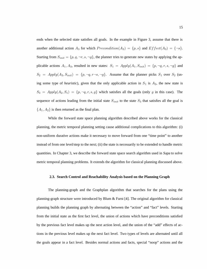
ends when the selected state satisfies all goals. In the example in Figure 3, assume that there is
another additional action A3 for which Precondition(A3) = {p, s} and Effect(A3) = {¬s}.
Starting from Sinit = {p, q,¬r, s,¬g}, the planner tries to generate new states by applying the ap-
plicable actions A1, A3, resulted in new states: S1 = Apply(A1, Sinit) = {p,¬q, r, s,¬g} and
S2 = Apply(A3, Sinit) = {p,¬q, r¬s,¬g}. Assume that the planner picks S1 over S2 (us-
ing some type of heuristic), given that the only applicable action in S1 is A2, the new state is
S3 = Apply(A2, S1) = {p,¬q, r, s, g} which satisfies all the goals (only g in this case). The
sequence of actions leading from the initial state Sinit to the state S3 that satisfies all the goal is
{A1, A2} is then returned as the final plan.
While the forward state space planning algorithm described above works for the classical
planning, the metric temporal planning setting cause additional complications to this algorithm: (i)
non-uniform durative actions make it necessary to move forward from one “time point” to another
instead of from one level/step to the next; (ii) the state is necessarily to be extended to handle metric
quantities. In Chapter 3, we describe the forward state space search algorithm used in Sapa to solve
metric temporal planning problems. It extends the algorithm for classical planning discussed above.
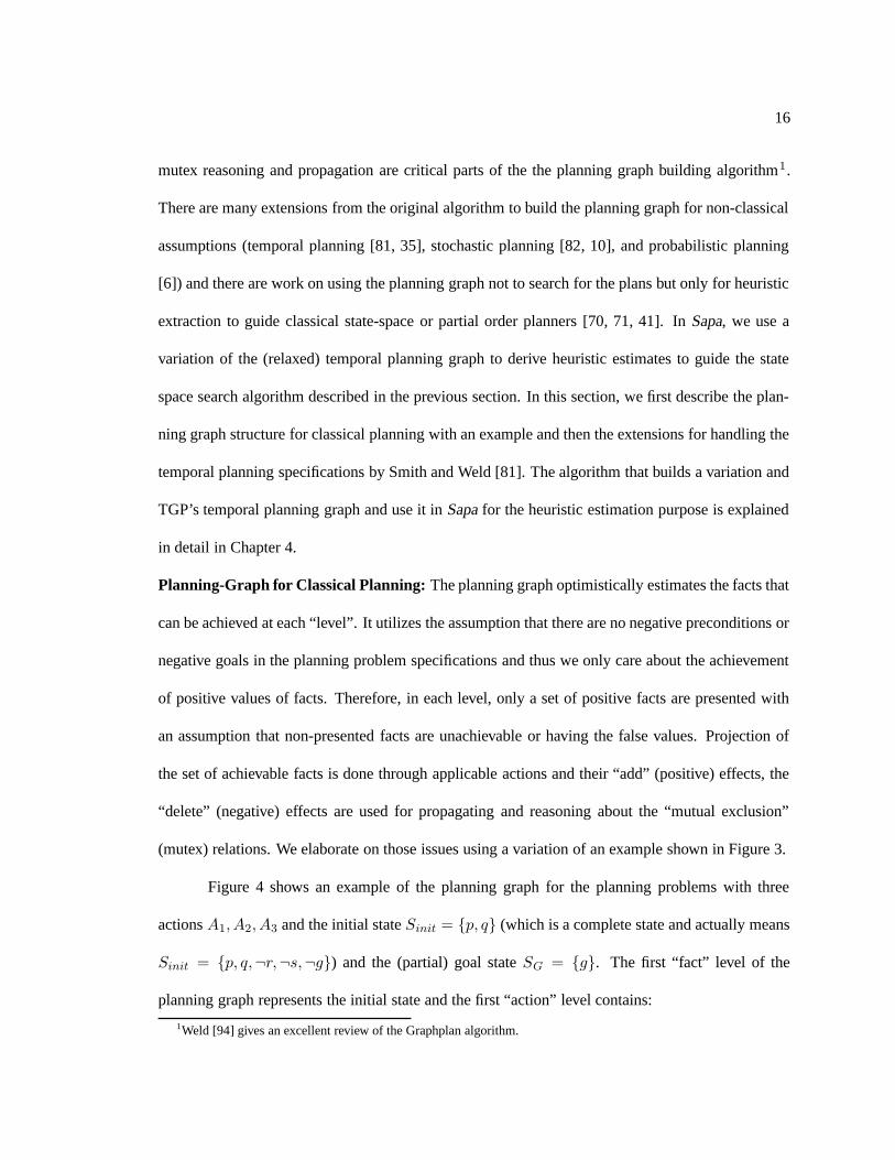
2.3. Search Control and Reachability Analysis based on the Planning Graph
The planning-graph and the Graphplan algorithm that searches for the plans using the
planning-graph structure were introduced by Blum & Furst [4]. The original algorithm for classical
planning builds the planning graph by alternating between the “action” and “fact” levels. Starting
from the initial state as the first fact level, the union of actions which have preconditions satisfied
by the previous fact level makes up the next action level, and the union of the “add” effects of ac-
tions in the previous level makes up the next fact level. Two types of levels are alternated until all
the goals appear in a fact level. Besides normal actions and facts, special “noop” actions and the
16
mutex reasoning and propagation are critical parts of the the planning graph building algorithm1 .
There are many extensions from the original algorithm to build the planning graph for non-classical
assumptions (temporal planning [81, 35], stochastic planning [82, 10], and probabilistic planning
[6]) and there are work on using the planning graph not to search for the plans but only for heuristic
extraction to guide classical state-space or partial order planners [70, 71, 41]. In Sapa, we use a
variation of the (relaxed) temporal planning graph to derive heuristic estimates to guide the state
space search algorithm described in the previous section. In this section, we first describe the plan-
ning graph structure for classical planning with an example and then the extensions for handling the
temporal planning specifications by Smith and Weld [81]. The algorithm that builds a variation and
TGP’s temporal planning graph and use it in Sapa for the heuristic estimation purpose is explained
in detail in Chapter 4.
Planning-Graph for Classical Planning: The planning graph optimistically estimates the facts that
can be achieved at each “level”. It utilizes the assumption that there are no negative preconditions or
negative goals in the planning problem specifications and thus we only care about the achievement
of positive values of facts. Therefore, in each level, only a set of positive facts are presented with
an assumption that non-presented facts are unachievable or having the false values. Projection of
the set of achievable facts is done through applicable actions and their “add” (positive) effects, the
“delete” (negative) effects are used for propagating and reasoning about the “mutual exclusion”
(mutex) relations. We elaborate on those issues using a variation of an example shown in Figure 3.
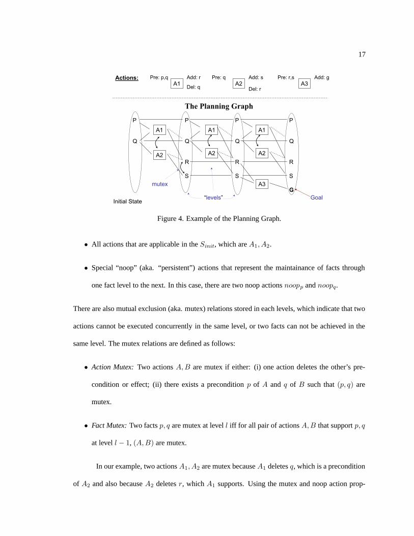
Figure 4 shows an example of the planning graph for the planning problems with three
actions A1, A2, A3 and the initial state Sinit = {p, q} (which is a complete state and actually means
Sinit = {p, q,¬r,¬s,¬g}) and the (partial) goal state SG = {g}. The first “fact” level of the
planning graph represents the initial state and the first “action” level contains:
1Weld [94] gives an excellent review of the Graphplan algorithm.
17
Actions:
A1Pre: p,q Add: r
Del: qA2
Pre: q Add: s
A3Pre: r,s Add: g
Del: r
The Planning Graph
P
Q
A1
A2
P
Q
R
S
A1
A2
P
Q
R
S
A1
A2
P
Q
R
S
G
A3
Initial StateGoal“levels”
mutex
Figure 4. Example of the Planning Graph.
• All actions that are applicable in the Sinit, which are A1, A2.
• Special “noop” (aka. “persistent”) actions that represent the maintainance of facts through
one fact level to the next. In this case, there are two noop actions noopp and noopq.
There are also mutual exclusion (aka. mutex) relations stored in each levels, which indicate that two
actions cannot be executed concurrently in the same level, or two facts can not be achieved in the
same level. The mutex relations are defined as follows:
• Action Mutex: Two actions A,B are mutex if either: (i) one action deletes the other’s pre-
condition or effect; (ii) there exists a precondition p of A and q of B such that (p, q) are
mutex.
• Fact Mutex: Two facts p, q are mutex at level l iff for all pair of actions A,B that support p, q
at level l − 1, (A,B) are mutex.
In our example, two actions A1, A2 are mutex because A1 deletes q, which is a precondition
of A2 and also because A2 deletes r, which A1 supports. Using the mutex and noop action prop-
18
agation rules listed above, the planning graph grows forward from the initial state by alternating
between fact and action levels. Each action level contains all applicable actions (i.e. all precondi-
tions appear pair-wise non-mutex in the previous fact level). Each fact level contains the union of
all effects of all actions (include noops) in the previous level. This process continues until all the
goals appear pair-wise non-mutex in a given fact level. In our example, the fact level 1 contains
{p, q, r, s} with new facts r, s supported by A1 and A2. These two new facts r, s are mutex because
A1 and A2 are mutex in the previous level, and thus action A3, which has preconditions (r, s), can
not be put in the action level 2. The fact level 3 contains the same facts with level 2, however, there
is no longer the mutex relation between r, s because there are two actions in level 2: A1 supporting
r and noops supporting s that are non-mutex. Finally, action A3 can be put in the action level 3 and
support the goal g at fact level 4. At this point, the planning graph building process stops. The plan-
ning graph along with the Graphplan algorithm that conduct search for the plans over the planning
graph is introduced by Blum & Furst in [4]; and the more detailed discussion can be found in [5].
Due to the fact that we only build the planning graph and use it for heuristic estimation (but not for
solution extracting) in Sapa, we do not discuss the Graphplan algorithm in this dissertation.
Extending the Planning Graph: Based on the observation that all facts and actions appear at
level k will also appear at later levels k + 1, and mutex relations if disappearing from level k then
also do not exist in level k + 1, the improved “bi-level” implementation of the original planning
graph structure described above only uses one fact and one action level. Each fact or action is then
associated with a number indicating the first level that fact/action appears in the planning graph.
Each fact/action mutex relation is also associated with the first level that it disappears from the
graph. This type of implementation is first used in the STAN [61] and IPP [54] planners and is
utilized in most recent planners that make use of the planning graph structure. In [81], Smith &
Weld argued that this bi-level planning graph structure is particularly suited for temporal planning
19
setting where there is no conceivable “level” but each action or fact is associated with the earliest
time point that it can be achieved (fact) or executed (action). For TGP’s temporal planning graph,
the noop actions are removed from the planning graph building phase but its mutex relations with
other actions are partially replaced by the mutex relations between actions and facts. The temporal
planning graph is also built forward starting from the initial state with time stamp t = 0, applicable
actions at time point t (with applicability condition similar to the classical planning scenario) are
put in the action level. Because different actions have different durations, we move forward not by
“level” but to the earliest time point that one of the activated action end. The details of the graph
building and mutex propagation process for temporal planning are discussed in [81].
Planning-graph as a basis for deriving heuristics: Besides the extensions to the planning graph
structure and the graphplan search algorithm to handle more expressive domains involving temporal
[81, 35], contingency [82], probability[6], and sensing [93] constraints, the planning graph and its
variations can also be used solely for heuristic estimate purpose to guide state-space (both backward
[70, 10], and forward [41, 25, 22]), POCL planners [71, 98], and local-search planner [33]. This can
be done by either: (i) using the levels at which goals appear in the planning graph to estimate
how difficult to achieve the goals; or (ii) use the planning graph to extract the “relaxed” plan.
For the first type of approach, in [70, 71], Nguyen et. al. discuss different frameworks to use
the goal-bearing level information and the positive/negative interactions between goals to derive
effective heuristics guiding backward state search and partial-order planner. The second approach of
extracting the relaxed plan mimics the Graphplan algorithm but avoids any backtracking due to the
mutex relations. Based on the causal structure encoded in the planning graph, the extraction process
starts by selecting actions to support top-level goals. When an action is selected, its preconditions
are added to the list of goals. This “backward” process stops when all the unachieved goals are
supported by the initial state. The set of collected action is then returned as a “relaxed plan” and
20
is used to estimate the real plan that can potentially achieve all the goals from the current initial
state. The name “relaxed plan” refers to the fact that mutual exclusion relations are ignored when
extracting the plan and thus the relaxed-plan may contain interacting actions that can not co-exist in
the non-relaxed valid plan.
To effectively extracting high-quality heuristics, there are several noteworthy variations of
the traditional planning graph, each one is suitable for a different search strategy. For the backward
planners (state-space regression, partial-order), where only one planning graph is needed for all
generated states2, the “serial” planning graph in which all pairs of actions (except noops) are made
mutex at every action level is more effective. For the forward planners, because each node rep-
resenting a different initial state and thus new planning graphs are needed, the “relaxed” planning
graph where the mutex relations are ignored is a common choice. In Sapa, we use the relaxed ver-
sion of the temporal planning graph introduced in TGP for the purpose of heuristic estimation. The
details of the planning graph building and heuristic extraction procedures for the PDDL2.1 Level 3
language are described in Chapter 4.
2This is due to the fact that all regression states share the same initial state, the starting point of the planning graph.
CHAPTER 3
Handling concurrent actions in a forward state space planner
The Sapa planner, the center piece of this dissertation, addresses planning problems that
involve durative actions, metric resources, and deadline goals. In this chapter, we describe how such
planning problems are represented and solved in Sapa. We will first describe the action and problem
representations in Section 3.1 and then will present the forward chaining state search algorithm used
by Sapa in Section 3.2.
3.1. Action Representation and Constraints
In this section, we will briefly describe our representation, which is an extension of the
action representation in PDDL2.1 Level 3 [28], the most expressive representation level used in
the Third International Planning Competition (IPC3). PDDL2.1 planning language extended PDDL
[63], which was used in the first planning competition (IPC1) in 1998 to represent the classical
planning problems following the STRIPS representation. It supports durative actions and continuous
value functions in several levels (with level 1 equal to PDDL1.0). For reference, we provide the
sample planning domain and problem files represented in PDDL and the extended version for metric
temporal planning in PDDL2.1 in the Appendix A.1 and A.2. Our extensions to PDDL2.1 Level 3
are: (i) interval preconditions; (ii) delayed effects that happen at time points other than action’s start
22
Tucson
Las Vegas
LA
Phoenix
Car1
Car2
Airplane
Train
Figure 5. The travel example
and end time points; and (iii) deadline goals.
Example: We shall start with an example to illustrate the action representation in a simple temporal
planning problem. This problem and its variations will be used as the running examples throughout
the next several chapters of this dissertation. Figure 5 shows graphically the problem description.
In this problem, a group of students in Tucson need to go to Los Angeles (LA). There are two
car rental options. If the students rent a faster but more expensive car (Car1), they can only go to
Phoenix (PHX) or Las Vegas (LV). However, if they decide to rent a slower but cheaper Car2, then
they can use it to drive to Phoenix or directly to LA. Moreover, to reach LA, the students can also
take a train from LV or a flight from PHX. In total, there are 6 movement actions in the domain:
drive-car1-tucson-phoenix (Dc1t→p, Dur = 1.0, Cost = 2.0), drive-car1-tucson-lv (Dc1
t→lv , Dur =
3.5, Cost = 3.0), drive-car2-tucson-phoenix (Dc2t→p, Dur = 1.5, Cost = 1.5), drive-car2-tucson-la
(Dc2t→la),Dur = 7.0, Cost = 6.0, fly-airplane-phoenix-la (Fp→la, Dur = 1.5, Cost = 6.0), and use-
train-lv-la (Tlv→la, Dur = 2.5, Cost = 2.5). Each move action A (by car/airplane/train) between
two cities X and Y requires the precondition that the students be at X (at(X)) at the beginning of
A. There are also two temporal effects: ¬at(X) occurs at the starting time point of A and at(Y ) at
the end time point of A. Driving and flying actions also consume different types of resources (e.g
fuel) at different rates depending on the specific car or airplane used. In addition, there are refueling
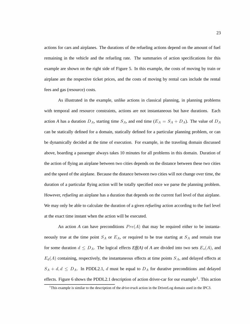
23
actions for cars and airplanes. The durations of the refueling actions depend on the amount of fuel
remaining in the vehicle and the refueling rate. The summaries of action specifications for this
example are shown on the right side of Figure 5. In this example, the costs of moving by train or
airplane are the respective ticket prices, and the costs of moving by rental cars include the rental
fees and gas (resource) costs.
As illustrated in the example, unlike actions in classical planning, in planning problems
with temporal and resource constraints, actions are not instantaneous but have durations. Each
action A has a duration DA, starting time SA, and end time (EA = SA + DA). The value of DA
can be statically defined for a domain, statically defined for a particular planning problem, or can
be dynamically decided at the time of execution. For example, in the traveling domain discussed
above, boarding a passenger always takes 10 minutes for all problems in this domain. Duration of
the action of flying an airplane between two cities depends on the distance between these two cities
and the speed of the airplane. Because the distance between two cities will not change over time, the
duration of a particular flying action will be totally specified once we parse the planning problem.
However, refueling an airplane has a duration that depends on the current fuel level of that airplane.
We may only be able to calculate the duration of a given refueling action according to the fuel level
at the exact time instant when the action will be executed.
An action A can have preconditions Pre(A) that may be required either to be instanta-
neously true at the time point SA or EA, or required to be true starting at SA and remain true
for some duration d ≤ DA. The logical effects Eff(A) of A are divided into two sets Es(A), and
Ed(A) containing, respectively, the instantaneous effects at time points SA, and delayed effects at
SA + d, d ≤ DA. In PDDL2.1, d must be equal to DA for durative preconditions and delayed
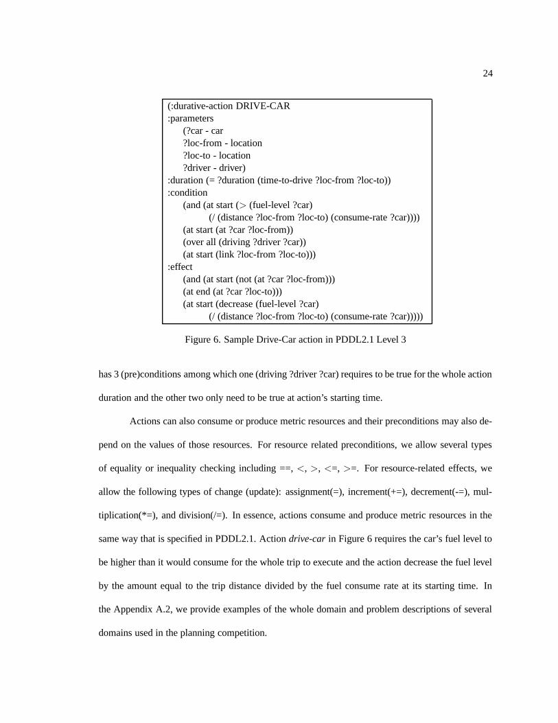
effects. Figure 6 shows the PDDL2.1 description of action driver-car for our example1. This action
1This example is similar to the description of the drive-truck action in the DriverLog domain used in the IPC3.
24
(:durative-action DRIVE-CAR:parameters
(?car - car?loc-from - location?loc-to - location?driver - driver)
:duration (= ?duration (time-to-drive ?loc-from ?loc-to)):condition
(and (at start (> (fuel-level ?car)(/ (distance ?loc-from ?loc-to) (consume-rate ?car))))
(at start (at ?car ?loc-from))(over all (driving ?driver ?car))(at start (link ?loc-from ?loc-to)))
:effect(and (at start (not (at ?car ?loc-from)))(at end (at ?car ?loc-to)))(at start (decrease (fuel-level ?car)
(/ (distance ?loc-from ?loc-to) (consume-rate ?car)))))
Figure 6. Sample Drive-Car action in PDDL2.1 Level 3
has 3 (pre)conditions among which one (driving ?driver ?car) requires to be true for the whole action
duration and the other two only need to be true at action’s starting time.
Actions can also consume or produce metric resources and their preconditions may also de-
pend on the values of those resources. For resource related preconditions, we allow several types
of equality or inequality checking including ==, <, >, <=, >=. For resource-related effects, we
allow the following types of change (update): assignment(=), increment(+=), decrement(-=), mul-
tiplication(*=), and division(/=). In essence, actions consume and produce metric resources in the
same way that is specified in PDDL2.1. Action drive-car in Figure 6 requires the car’s fuel level to
be higher than it would consume for the whole trip to execute and the action decrease the fuel level
by the amount equal to the trip distance divided by the fuel consume rate at its starting time. In
the Appendix A.2, we provide examples of the whole domain and problem descriptions of several
domains used in the planning competition.
25
3.2. A Forward Chaining Search Algorithm for Metric Temporal Planning
While variations of the metric temporal action representation scheme described in the last
section have been used in partial order temporal planners such as IxTeT [37] and Zeno [75], Bacchus
and Ady [1] were the first to propose a forward chaining algorithm capable of using this type of
action representation and still allow concurrent execution of actions in the plan. We adopt and
generalize their search algorithm in Sapa. The main idea here is to separate the decisions of “which
action to apply” and “at what time point to apply the action.” Regular progression search planners
apply an action in the state resulting from the application of all the actions in the current prefix plan.
This means that the start time of the new action is after the end time of the last action in the prefix,
and the resulting plan will not allow concurrent execution. In contrast, Sapa non-deterministically
considers (i) application of new actions at the current time stamp (where presumably other actions
have already been applied; thus allowing concurrency) and (ii) advancement of the current time
stamp.
Sapa’s search is thus conducted through the space of time stamped states. We define a time
stamped state S as a tuple S = (P,M,Π, Q, t) consisting of the following structure:
• P = (〈pi, ti〉 | ti ≤ t) is a set of predicates pi that are true at t and ti is the last time instant
at which they were achieved.
• M is a set of values for all continuous functions, which may change over the course of plan-
ning. Functions are used to represent the metric-resources and other continuous values. Ex-
amples of functions are the fuel levels of vehicles.
• Π is a set of persistent conditions, such as durative preconditions, that need to be protected
during a specific period of time.
26
• Q is an event queue containing a set of updates each scheduled to occur at a specified time in
the future. An event e can do one of three things: (1) change the True/False value of some
predicate, (2) update the value of some function representing a metric-resource, or (3) end the
persistence of some condition.
• t is the time stamp of S
In this dissertation, unless noted otherwise, when we say “state” we mean a time stamped
state. Note that a time stamped state with a stamp t not only describes the expected snapshot of the
world at time t during execution (as done in classical progression planners), but also the delayed
(but inevitable) effects of the commitments that have been made by (or before) time t.
If there is no exogenous events, the initial state Sinit has time stamp t = 0 and has an empty
event queue and empty set of persistent conditions. If the problem also involves a set of exogenous
events (in the form of timed initial facts discussed in PDDL2.2), then the initial state Sinit’s event
queue is made up by the collection of those events. It is completely specified in terms of function
and predicate values. The goals are represented by a set of 2-tuples G = (〈p1, t1〉...〈pn, tn〉) where
pi is the ith goal and ti is the time instant by which pi needs to be achieved. Note that PDDL2.1
does not allow the specification of goal deadline constraints.
Goal Satisfaction: The state S = (P,M,Π, Q, t) subsumes (entails) the goal G if for each 〈pi, ti〉 ∈
G either:
1. ∃〈pi, tj〉 ∈ P , tj < ti and there is no event in Q that deletes pi.
2. ∃e ∈ Q that adds pi at time instant te < ti, and there is no event in Q that deletes pi.2
Action Applicability: An action A is applicable in state S = (P,M,Π, Q, t) if:
2In practice, conflicting events are never put on Q

27
1. All logical (pre)conditions of A are satisfied by P.
2. All metric resource (pre)conditions of A are satisfied by M. (For example, if the condition to
execute an action A = move(truck,A,B) is fuel(truck) > 500 then A is executable in S
if the value v of fuel(truck) in M satisfies v > 500.)
3. A’s effects do not interfere with any persistent condition in Π and any event in Q.
4. There is no event in Q that interferes with persistent preconditions of A.
Interference: Interference is defined as the violation of any of the following conditions:
1. Action A should not add any event e that causes p if there is another event currently in Q that
causes ¬p. Thus, there is never a state in which there are two events in the event queue that
cause opposite effects.
2. If A deletes p and p is protected in Π until time point tp, then A should not delete p before tp.
3. If A has a persistent precondition p, and there is an event that gives ¬p, then that event should
occur after A terminates.
4. A should not change the value of any function which is currently accessed by another un-
terminated action3 . Moreover, A also should not access the value of any function that is
currently changed by an unterminated action.
At first glance, the first interference condition seems to be overly strong. However, we
argue that it is necessary to keep underlying processes that cause contradicting state changes from
overlapping each other. For example, suppose that we have two actions A1 = build house, A2 =
3Unterminated actions are the ones that started before the time point t of the current state S but have not yet finishedat t.
28
destroy house and Dur(A1) = 10, Dur(A2) = 7. A1 has effect has house and A2 has effect
¬has house at their end time points. Assuming that A1 is applied at time t = 0 and added an event
e = Add(has house) at t = 10. If we are allowed to apply A2 at time t = 0 and add a contradicting
event e′ = Delete(has house) at t = 7, then it is unreasonable to believe that we will still have a
house at time t = 10 anymore. Thus, even though in our current action modeling, state changes that
cause has house and ¬has house look as if they happen instantaneously at the actions’ end time
points, there are underlying processes (build/destroy house) that span the whole action durations to
make them happen. To prevent those contradicting processes from overlapping with each other, we
employ the conservative approach of not letting Q contain contradicting effects.4
When we apply an action A to a state S = (P,M,Π, Q, t), all instantaneous effects of A
will be immediately used to update the predicate list P and metric resources database M of S. A’s
persistent preconditions and delayed effects will be put into the persistent condition set Π and event
queue Q of S.
Besides the normal actions, we will have a special action called advance-time which we
use to advance the time stamp of S to the time instant te of the earliest event e in the event queue
Q of S. The advance-time action will be applicable in any state S that has a non-empty event queue.
Upon applying this action, the state S gets updated according to all the events in the event queue
that are scheduled to occur at te. Note that we can apply multiple non-interfering actions at a given
time point before applying the special advance-time action. This allows for concurrency in the final
plan.
4It may be argued that there are cases in which there is no process to give certain effect, or there are situations in whichthe contradicting processes are allowed to overlap. However, without the ability to explicitly specify the processes andtheir characteristics in the action representation, we currently decided to go with the conservative approach. We shouldalso mention that the interference relations above do not preclude a condition from being established and deleted in thecourse of a plan as long as the processes involved in establishment and deletion do not overlap. In the example above, itis legal to first build the house and then destroy it.
29
State Queue: SQ={Sinit}while SQ6={}
S:= Dequeue(SQ)Nondeterministically select A applicable in S
/* A can be advance-time action */S’ := Apply(A,S)if S’ satisfies G then PrintSolutionelse Enqueue(S’,SQ)
end while;
Figure 7. Main search algorithm
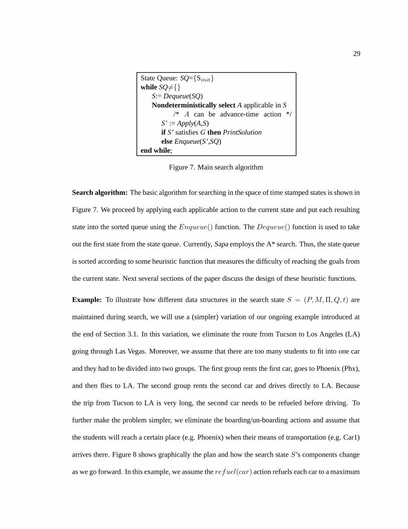
Search algorithm: The basic algorithm for searching in the space of time stamped states is shown in
Figure 7. We proceed by applying each applicable action to the current state and put each resulting
state into the sorted queue using the Enqueue() function. The Dequeue() function is used to take
out the first state from the state queue. Currently, Sapa employs the A* search. Thus, the state queue
is sorted according to some heuristic function that measures the difficulty of reaching the goals from
the current state. Next several sections of the paper discuss the design of these heuristic functions.
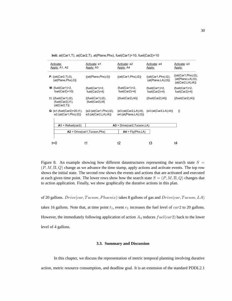
Example: To illustrate how different data structures in the search state S = (P,M,Π, Q, t) are
maintained during search, we will use a (simpler) variation of our ongoing example introduced at
the end of Section 3.1. In this variation, we eliminate the route from Tucson to Los Angeles (LA)
going through Las Vegas. Moreover, we assume that there are too many students to fit into one car
and they had to be divided into two groups. The first group rents the first car, goes to Phoenix (Phx),
and then flies to LA. The second group rents the second car and drives directly to LA. Because
the trip from Tucson to LA is very long, the second car needs to be refueled before driving. To
further make the problem simpler, we eliminate the boarding/un-boarding actions and assume that
the students will reach a certain place (e.g. Phoenix) when their means of transportation (e.g. Car1)
arrives there. Figure 8 shows graphically the plan and how the search state S’s components change
as we go forward. In this example, we assume the refuel(car) action refuels each car to a maximum
30
Init: at(Car1,T), at(Car2,T), at(Plane,Phx), fuel(Car1)=10, fuel(Car2)=10
Activate: e4
Apply:
Activate: e1
Apply: A3
Activate:
Apply: A1, A2
Activate: e2
Apply: A4
Activate: e3
Apply:
{(at(Car1,Phx),t2),
(at(Plane,LA),t3),
(at(Car2,LA),t4)}
P: {(at(Car2,T),0),
(at(Plane,Phx),0)}
{(at(Plane,Phx),0)} {(at(Car1,Phx),t2)} {(at(Car1,Phx),t2),
(at(Plane,LA),t3)}
M: {fuel(Car1)=2,
fuel(Car2)=10}
{fuel(Car1)=2,
fuel(Car2)=4}{fuel(Car1)=2,
fuel(Car2)=4}
{fuel(Car1)=2,
fuel(Car2)=4}
{fuel(Car1)=2,
fuel(Car2)=4}
{(fuel(Car2),t4)}{(fuel(Car2),t4)} {(fuel(Car2),t4)}{(fuel(Car1),t2),
(fuel(Car2),t4}
: {(fuel(Car1),t2),
(fuel(Car2),t1),
(at(Car2,T)}
Q: {e1:(fuel(Car2)=20,t1),
e2:(at(Car1,Phx),t2)}
{}{e3:(at(Car2,LA),t4),
e4:(at(Plane,LA),t3)}
{e3:(at(Car2,LA),t4)}{e2:(at(Car1,Phx),t2),
e3:(at(Car2,LA),t4)}
A1 = Refuel(car2) A3 = Drive(car2,Tucson,LA)
A2 = Drive(car1,Tucson,Phx) A4 = Fly(Phx,LA)
t=0 t1 t2 t3 t4
Figure 8. An example showing how different datastructures representing the search state S =(P,M,Π, Q) change as we advance the time stamp, apply actions and activate events. The top rowshows the initial state. The second row shows the events and actions that are activated and executedat each given time point. The lower rows show how the search state S = (P,M,Π, Q) changes dueto action application. Finally, we show graphically the durative actions in this plan.
of 20 gallons. Drive(car, Tucson, Phoenix) takes 8 gallons of gas and Drive(car, Tucson, LA)
takes 16 gallons. Note that, at time point t1, event e1 increases the fuel level of car2 to 20 gallons.
However, the immediately following application of action A3 reduces fuel(car2) back to the lower
level of 4 gallons.
3.3. Summary and Discussion
In this chapter, we discuss the representation of metric temporal planning involving durative
action, metric resource consumption, and deadline goal. It is an extension of the standard PDDL2.1
31
Level 3 planning language. We also describe the forward search algorithm in Sapa that produces
fixed-time temporal parallel plans using this representation.
In the future, we want to make Sapa support a richer set of temporal and resource constraints
such as:
• Time-dependent action duration/cost and resource consumption (e.g. driving from office to
the airport takes longer time and is costlier during rush hour than at less-traffic time).
• Supporting continuous change during action duration (PDDL2.1 Level 4).
For both of those issues, due to the forward state space search algorithm where the total
knowledge of the world is available at each action’s starting time, unlike backward planner, it is not
hard to extend the state representation and consistency checking routine to handle those additional
constraints. From the technical point of view, for the first issue, we need a better time-related
estimation for actions in the partial plan (g value) and in the relaxed plan (h value). For the g value,
we are currently investigating an approach of “online partialization” to push every newly added
action’s starting time as early as possible. This is done by maintaining an additional causal structure
between actions in the partial plan. For the h value, better estimation of the starting time of actions
that can potentially in the relaxed plan is a plus. We will elaborate it in the later part of this chapter
(dedicated for heuristic improvement). For the second issue of supporting continuous changes, we
plan to explicitly keep a resource profile for each resource that is currently under change according
to some functions in the partial plan.
CHAPTER 4
Heuristics based on Propagated Cost-Functions over the Relaxed
Planning Graph
A critical part of any planner is its heuristic estimate component. In forward state space
planners, quality of the heuristic is basically decided by the ability to select lower cost actions that
lead to states closer to the goals. Without good heuristic control, it would be nearly impossible for
blind search to find a plan in reasonable time. Let’s assume that the branching factor of a normal
planning problem is 20 and we have a very fast computer that can examine 100,000 nodes per
second. Then, to find a solution of length 5, we need to search about 32 seconds, a solution of
length 10 would need more than 3 years and a solution of length 20 would need about 318 years to
find. Nevertheless, good heuristics enable state-of-the-art planners to find solutions with hundred of
actions in minutes.
In this chapter, we discuss the issue of deriving heuristics, that are sensitive to both time
and cost, to guide Sapa’s search algorithm. An important challenge in finding heuristics to support
multi-objective search, as illustrated by the example below, is that the cost and temporal aspects of
a plan are often inter-dependent. Therefore, in this chapter, we introduce the approach of tracking
the costs of achieving goals and executing actions in the plan as functions of time. The propagated
cost functions can then be used to derive the heuristic values to guide the search in Sapa.
33
Example: Consider a simpler version of our ongoing example. Suppose that we need to go from
Tucson to Los Angeles and have two transport options: (i) rent a car and drive from Tucson to Los
Angeles in one day for $100 or (ii) take a shuttle to the Phoenix airport and fly to Los Angeles in
3 hours for $200. The first option takes more time (higher makespan) but less money, while the
second one clearly takes less time but is more expensive. Depending on the specific weights the
user gives to each criterion, she may prefer the first option over the second or vice versa. Moreover,
the user’s decision may also be influenced by other constraints on time and cost that are imposed on
the final plan. For example, if she needs to be in Los Angeles in six hours, then she may be forced
to choose the second option. However, if she has plenty of time but limited budget, then she may
choose the first option.
The simple example above shows that makespan and execution cost, while nominally inde-
pendent of each other, are nevertheless related in terms of the overall objectives of the user and the
constraints on a given planning problem. More specifically, for a given makespan threshold (e.g.
to be in LA within six hours), there is a certain estimated solution cost tied to it (shuttle fee and
ticket price to LA) and analogously for a given cost threshold there is a certain estimated time tied
to it. Thus, in order to find plans that are good with respect to both cost and makespan, we need to
develop heuristics that track cost of a set of (sub)goals as a function of time.
Given that the planning graph is an excellent structure to represent the relation between
facts and actions [70], we will use a temporal version of the planning graph structure, such as
that introduced in TGP [81], as a substrate for propagating the cost information. We starts with
Section 4.1 containing a brief discussion of the data structures used for the cost propagation process.
We then continue with the details of the propagation process in Section 4.2, and the criteria used
to terminate the propagation in Section 4.3. Section 4.4 discusses how the cost functions are used
to extract heuristic values. We finish with Section 4.5 on adjustment techniques to improve the

34
heuristic quality.
4.1. The Temporal Planning Graph Structure
We now adapt the notion of temporal planning graphs, introduced by Smith & Weld in [81],
to our action representation. The temporal planning graph for a given problem is a bi-level graph,
with one level containing all facts, and the other containing all actions in the planning problem.
Each fact has links to all actions supporting it, and each action has links to all facts that belong to
its precondition and effect lists.1 Actions are durative and their effects are represented as events that
occur at some time between the action’s start and end time points. As we will see in more detail
in the later parts of this section, we build the temporal planning graph by incrementally increasing
the time (makespan value) of the graph. At a given time point t, an action A is activated if all
preconditions of A can be achieved at t. To support the delayed effects of the activated actions (i.e.,
effects that occur at the future time points beyond t), we also maintain a global event queue for
the entire graph, Q = {e1, e2, ...en} sorted in the increasing order of event time. The event queue
for the temporal graph differs from the event queue for the search state (discussed in the previous
section) in the following ways:
• It is associated with the whole planning graph (rather than with each single state).
• It only contains the positive events. Specifically, the negative effects and the resource-related
effects of the actions are not entered in to the graph’s queue.
• All the events in Q have event costs associated with each individual event (see below).
1The bi-level representation has been used in classical planning to save time and space [61], but as Smith & Weld [81]show, it makes even more sense in temporal planning domains because there is actually no notion of level. All we haveare a set of fact/action nodes, each one encoding information such as the earliest time point at which the fact/action canbe achieved/executed, and the lowest cost incurred to achieve them.
35
Each event in Q is a 4-tuple e = 〈f, t, c, A〉 in which: (1) f is the fact that e will add; (2) t
is the time point at which the event will occur; and (3) c is the cost incurred to enable the execution
of action A which causes e. For each action A, we introduce a cost function C(A, t) = v to specify
the estimated cost v that we incur to enable A’s execution at time point t. In other words, C(A, t)
is the estimate of the cost incurred to achieve all of A’s preconditions at time point t. Moreover,
each action will also have an execution cost (Cexec(A)), which is the cost incurred in executing A
(e.g. ticket price for the fly action, gas cost for driving a car). For each fact f , a similar cost function
C(f, t) = v specifies the estimated cost v incurred to achieve f at time point t (e.g. cost incurred
to be in Los Angeles in 6 hours). We also need an additional function SA(f, t) = Af to specify the
action Af that can be used to support f with cost v at time point t.
Since we are using a “relaxed” planning graph that is constructed ignoring delete effects,
and resource effects, the derived heuristics will not be sensitive to negative interactions and resource
restrictions2 . In Sections 4.5 we discuss how the heuristic measures are adjusted to take these
interactions into account.
4.2. Cost Propagation Procedure
As mentioned above, our general approach is to propagate the estimated costs incurred
to achieve facts and actions from the initial state. As a first step, we need to initialize the cost
functions C(A, t) and C(f, t) for all facts and actions. For a given initial state Sinit, let F =
{f1, f2...fn} be the set of facts that are true at time point tinit and {(f ′1, t1), ...(f
′m, tm)}, be a set
of outstanding positive events which specify the addition of facts f ′i at time points ti > tinit. We
introduce a dummy action Ainit to represent Sinit where Ainit (i) requires no preconditions; (ii) has
2In the original Graphplan algorithm [4], there is a process of propagating mutex information, which captures thenegative interactions between different propositions and actions occurring at the same time (level). To reduce the heuristiccomputation cost, we will neglect the mutex propagation and will discuss the propagation process in the context of therelaxed problem in which the delete effects of actions, which cause the mutex relations, are ignored.
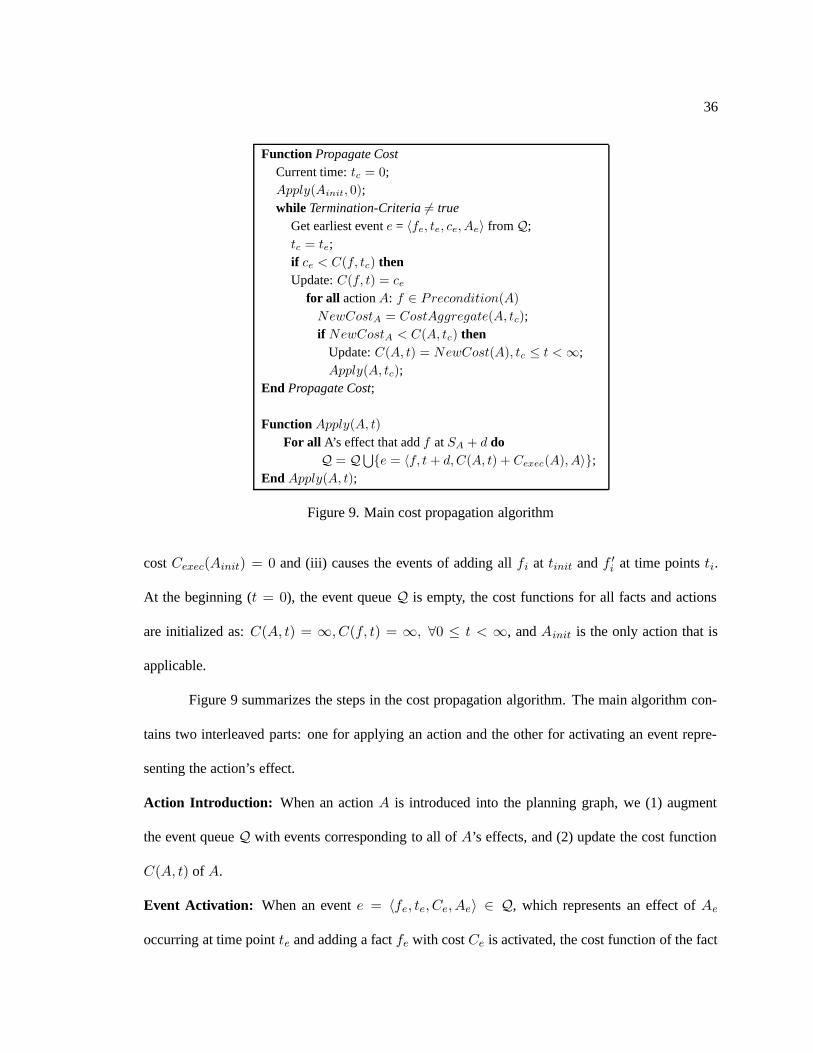
36
Function Propagate CostCurrent time: tc = 0;Apply(Ainit, 0);while Termination-Criteria 6= true
Get earliest event e = 〈fe, te, ce, Ae〉 fromQ;tc = te;if ce < C(f, tc) thenUpdate: C(f, t) = ce
for all action A: f ∈ Precondition(A)
NewCostA = CostAggregate(A, tc);if NewCostA < C(A, tc) then
Update: C(A, t) = NewCost(A), tc ≤ t <∞;Apply(A, tc);
End Propagate Cost;
Function Apply(A, t)
For all A’s effect that add f at SA + d doQ = Q
⋃
{e = 〈f, t + d, C(A, t) + Cexec(A), A〉};End Apply(A, t);
Figure 9. Main cost propagation algorithm
cost Cexec(Ainit) = 0 and (iii) causes the events of adding all fi at tinit and f ′i at time points ti.
At the beginning (t = 0), the event queue Q is empty, the cost functions for all facts and actions
are initialized as: C(A, t) = ∞, C(f, t) = ∞, ∀0 ≤ t < ∞, and Ainit is the only action that is
applicable.
Figure 9 summarizes the steps in the cost propagation algorithm. The main algorithm con-
tains two interleaved parts: one for applying an action and the other for activating an event repre-
senting the action’s effect.
Action Introduction: When an action A is introduced into the planning graph, we (1) augment
the event queue Q with events corresponding to all of A’s effects, and (2) update the cost function
C(A, t) of A.
Event Activation: When an event e = 〈fe, te, Ce, Ae〉 ∈ Q, which represents an effect of Ae
occurring at time point te and adding a fact fe with cost Ce is activated, the cost function of the fact
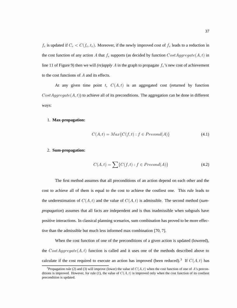
37
fe is updated if Ce < C(fe, te). Moreover, if the newly improved cost of fe leads to a reduction in
the cost function of any action A that fe supports (as decided by function CostAggregate(A, t) in
line 11 of Figure 9) then we will (re)apply A in the graph to propagate fe’s new cost of achievement
to the cost functions of A and its effects.
At any given time point t, C(A, t) is an aggregated cost (returned by function
CostAggregate(A, t)) to achieve all of its preconditions. The aggregation can be done in different
ways:
1. Max-propagation:
C(A, t) = Max{C(f, t) : f ∈ Precond(A)} (4.1)
2. Sum-propagation:
C(A, t) =∑
{C(f, t) : f ∈ Precond(A)} (4.2)
The first method assumes that all preconditions of an action depend on each other and the
cost to achieve all of them is equal to the cost to achieve the costliest one. This rule leads to
the underestimation of C(A, t) and the value of C(A, t) is admissible. The second method (sum-
propagation) assumes that all facts are independent and is thus inadmissible when subgoals have
positive interactions. In classical planning scenarios, sum combination has proved to be more effec-
tive than the admissible but much less informed max combination [70, 7].
When the cost function of one of the preconditions of a given action is updated (lowered),
the CostAggregate(A, t) function is called and it uses one of the methods described above to
calculate if the cost required to execute an action has improved (been reduced).3 If C(A, t) has
3Propagation rule (2) and (3) will improve (lower) the value of C(A, t) when the cost function of one of A’s precon-ditions is improved. However, for rule (1), the value of C(A, t) is improved only when the cost function of its costliestprecondition is updated.
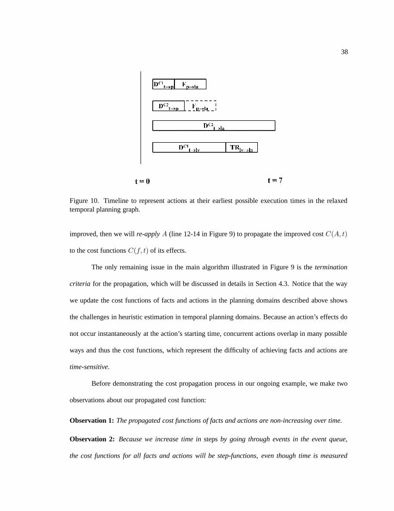
38
Figure 10. Timeline to represent actions at their earliest possible execution times in the relaxedtemporal planning graph.
improved, then we will re-apply A (line 12-14 in Figure 9) to propagate the improved cost C(A, t)
to the cost functions C(f, t) of its effects.
The only remaining issue in the main algorithm illustrated in Figure 9 is the termination
criteria for the propagation, which will be discussed in details in Section 4.3. Notice that the way
we update the cost functions of facts and actions in the planning domains described above shows
the challenges in heuristic estimation in temporal planning domains. Because an action’s effects do
not occur instantaneously at the action’s starting time, concurrent actions overlap in many possible
ways and thus the cost functions, which represent the difficulty of achieving facts and actions are
time-sensitive.
Before demonstrating the cost propagation process in our ongoing example, we make two
observations about our propagated cost function:
Observation 1: The propagated cost functions of facts and actions are non-increasing over time.
Observation 2: Because we increase time in steps by going through events in the event queue,
the cost functions for all facts and actions will be step-functions, even though time is measured
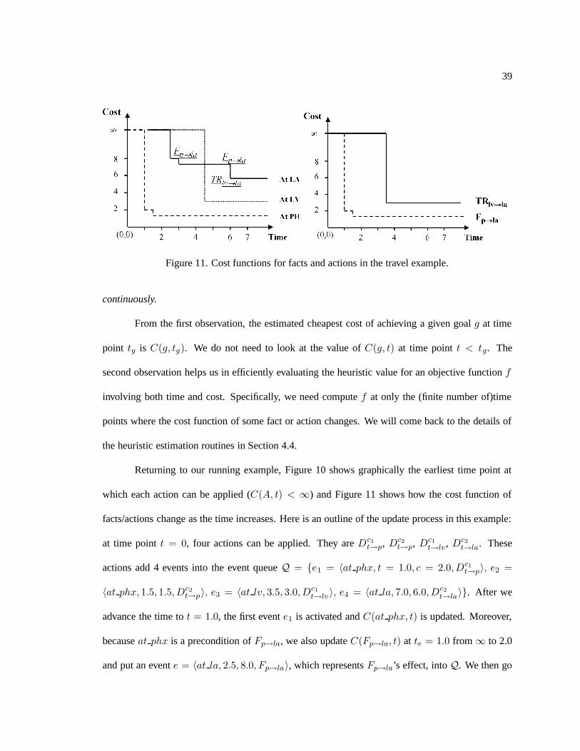
39
Figure 11. Cost functions for facts and actions in the travel example.
continuously.
From the first observation, the estimated cheapest cost of achieving a given goal g at time
point tg is C(g, tg). We do not need to look at the value of C(g, t) at time point t < tg. The
second observation helps us in efficiently evaluating the heuristic value for an objective function f
involving both time and cost. Specifically, we need compute f at only the (finite number of)time
points where the cost function of some fact or action changes. We will come back to the details of
the heuristic estimation routines in Section 4.4.
Returning to our running example, Figure 10 shows graphically the earliest time point at
which each action can be applied (C(A, t) < ∞) and Figure 11 shows how the cost function of
facts/actions change as the time increases. Here is an outline of the update process in this example:
at time point t = 0, four actions can be applied. They are Dc1t→p, Dc2
t→p, Dc1t→lv , Dc2
t→la. These
actions add 4 events into the event queue Q = {e1 = 〈at phx, t = 1.0, c = 2.0, Dc1t→p〉, e2 =
〈at phx, 1.5, 1.5, Dc2t→p〉, e3 = 〈at lv, 3.5, 3.0, Dc1
t→lv 〉, e4 = 〈at la, 7.0, 6.0, Dc2t→la〉}. After we
advance the time to t = 1.0, the first event e1 is activated and C(at phx, t) is updated. Moreover,
because at phx is a precondition of Fp→la, we also update C(Fp→la, t) at te = 1.0 from∞ to 2.0
and put an event e = 〈at la, 2.5, 8.0, Fp→la〉, which represents Fp→la’s effect, into Q. We then go
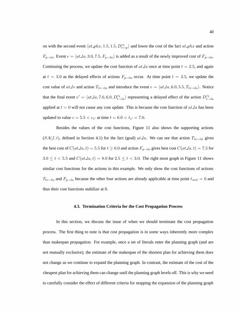
40
on with the second event 〈at phx, 1.5, 1.5, Dc2t→p〉 and lower the cost of the fact at phx and action
Fp→la. Event e = 〈at la, 3.0, 7.5, Fp→la〉 is added as a result of the newly improved cost of Fp→la.
Continuing the process, we update the cost function of at la once at time point t = 2.5, and again
at t = 3.0 as the delayed effects of actions Fp→la occur. At time point t = 3.5, we update the
cost value of at lv and action Tlv→la and introduce the event e = 〈at la, 6.0, 5.5, Tlv→la〉. Notice
that the final event e′ = 〈at la, 7.0, 6.0, Dc2t→la〉 representing a delayed effect of the action Dc2
t→la
applied at t = 0 will not cause any cost update. This is because the cost function of at la has been
updated to value c = 5.5 < ce′ at time t = 6.0 < te′ = 7.0.
Besides the values of the cost functions, Figure 11 also shows the supporting actions
(SA(f, t), defined in Section 4.1) for the fact (goal) at la. We can see that action Tlv→la gives
the best cost of C(at la, t) = 5.5 for t ≥ 6.0 and action Fp→la gives best cost C(at la, t) = 7.5 for
3.0 ≤ t < 5.5 and C(at la, t) = 8.0 for 2.5 ≤ t < 3.0. The right most graph in Figure 11 shows
similar cost functions for the actions in this example. We only show the cost functions of actions
Tlv→la and Fp→la because the other four actions are already applicable at time point tinit = 0 and
thus their cost functions stabilize at 0.
4.3. Termination Criteria for the Cost Propagation Process
In this section, we discuss the issue of when we should terminate the cost propagation
process. The first thing to note is that cost propagation is in some ways inherently more complex
than makespan propagation. For example, once a set of literals enter the planning graph (and are
not mutually exclusive), the estimate of the makespan of the shortest plan for achieving them does
not change as we continue to expand the planning graph. In contrast, the estimate of the cost of the
cheapest plan for achieving them can change until the planning graph levels off. This is why we need
to carefully consider the effect of different criteria for stopping the expansion of the planning graph

41
on the accuracy of the cost estimates. The first intuition is that we should not stop the propagation
when there exist top level goals for which the cost of achievement is still infinite (unreached goal).
On the other hand, given our objective function of finding the cheapest way to achieve the goals, we
need not continue the propagation when there is no chance that we can improve the cost of achieving
the goals. From those intuitions, following are several rules that can be used to determine when to
terminate propagation:
Deadline termination: The propagation should stop at a time point t if: (1) ∀ goal G :
Deadline(G) ≤ t, or (2) ∃ goal G : (Deadline(G) < t) ∧ (C(G, t) =∞).
The first rule governs the hard constraints on the goal deadlines. It implies that we should
not propagate beyond the latest goal deadline (because any cost estimation beyond that point is
useless), or we can not achieve some goal by its deadline.
With the observation that the propagated costs can change only if we still have some events
left in the queue that can possibly change the cost functions of a specific propositions, we have the
second general termination rule regarding the propagation:
Fix-point termination: The propagation should stop when there are no more events that can de-
crease the cost of any proposition.
The second rule is a qualification for reaching the fix-point in which there is no gain on the
cost function of any fact or action. It is analogous to the idea of growing the planning graph until it
levels-off in classical planning.
Stopping the propagation according to the two general rules above leads us to the best (low-
est value) achievable cost estimation for all propositions given a specific initial state. However, there
are several situations in which we may want to stop the propagation process earlier. First, propaga-
tion until the fix-point, where there is no gain on the cost function of any fact or action, would be
too costly [70]. Second, the cost functions of the goals may reach the fix-point long before the full
42
propagation process is terminated according to the general rules discussed above, where the costs
of all propositions and actions stabilize.
Given the above motivations, we introduce several different criteria to stop the propagation
earlier than is entailed by the fix-point computation:
Zero-lookahead approximation: Stop the propagation at the earliest time point t where all the
goals are reachable (C(G, t) <∞).
One-lookahead approximation: At the earliest time point t where all the goals are reachable,
execute all the remaining events in the event queue and stop the propagation.
One-lookahead approximation looks ahead one step in the (future) event queues when one
path to achieve all the goals under the relaxed assumption is guaranteed and hopes that executing
all those events would explicate some cheaper path to achieve all goals.4
Zero and one-lookahead are examples of a more general k-lookahead approximation, in
which extracting the heuristic value as soon as all the goals are reachable corresponds to zero-
lookahead and continuing to propagate until the fix-point corresponds to the infinite (full) looka-
head. The rationale behind the k-lookahead approximation is that when all the goals appear, which
is an indication that there exists at least one (relaxed) solution, then we will look ahead one or more
steps to see if we can achieve some extra improvement in the cost of achieving the goals (and thus
lead to a lower cost solution).5
Coming back to our travel example, zero-lookahead stops the propagation process at the
time point t = 2.5 and the goal cost is C(in la, 2.5) = 8.0. The action chain giving that cost
is {Dc1t→p, Fp→la}. With one-lookahead, we find the lowest cost for achieving the goal in la is
4Note that even if none of those events is directly related to the goals, their executions can still indirectly lead to better(cheaper) path to reach all the goals.
5For backward planners where we only need to run the propagation one time, infinite-lookahead or higher levels oflookahead may pay off, while in forward planners where we need to evaluate the cost of goals for each single search state,lower values of k may be more appropriate.
43
C(in la, 7.0) = 6.0 and it is given by the action (Dc2t→la). With two-lookahead approximation,
the lowest cost for in la is C(in la, 6.0) = 5.5 and it is achieved by cost propagation through
the action set {(Dc1t→lv, Tlv→la)}. In this example, two-lookahead has the same effect as the fix-
point propagation (infinite lookahead) if the deadline to achieve in la is later than t = 6.0. If it is
earlier, say Deadline(in la) = 5.5, then the one-lookahead will have the same effect as the infinite-
lookahead option and gives the cost of C(in la, 3.0) = 7.5 for the action chain {Dc2t→phx, Fphx→la}.
4.4. Heuristics based on Propagated Cost Functions
Once the propagation process terminates, the time-sensitive cost functions contain sufficient
information to estimate any makespan and cost-based heuristic value of a given state. Specifically,
suppose the planning graph is grown from a state S. Then the cost functions for the set of goals
G = {(g1, t1), (g2, t2)...(gn, tn)}, ti = Deadline(gi) can be used to derive the following estimates:
• The minimum makespan estimate T (PS) for a plan starting from S is given by the earliest
time point τ0 at which all goals are reached with finite cost C(g, t) <∞.
• The minimum/maximum/summation estimate of slack Slack(PS) for a plan starting from S
is given by the minimum/maximum/summation of the distances between the time point at
which each goal first appears in the temporal planning graph and the deadline of that goal.
• The minimum cost estimate, (C(g, deadline(g))), of a plan starting from a state S and achiev-
ing a set of goals G, C(PS , τ∞), can be computed by aggregating the cost estimates for
achieving each of the individual goals at their respective deadlines.6 Notice that we use τ∞ to
6If we consider G as the set of preconditions for a dummy action that represents the goal state, then we can use anyof the propagation rules (max/sum) discussed in Section 4.2 to directly estimate the total cost of achieving the goals fromthe given initial state.
44
denote the time point at which the cost propagation process stops. Thus, τ∞ is the time point
at which the cost functions for all individual goals C(f, τ∞) have their lowest value.
• For each value t : τ0 < t < τ∞, the cost estimate of a plan C(PS , t), which can achieve goals
within a given makespan limit of t, is the aggregation of the values C(gi, t) of goals gi.
The makespan and the cost estimates of a state can be used as the basis for deriving heuris-
tics. The specific way these estimates are combined to compute the heuristic values does of course
depend on what the user’s ultimate objective function is. In the general case, the objective would be
a function f(C(PS), T (PS)) involving both the cost (C(PS)) and makespan (T (PS)) values of the
plan. Suppose that the objective function is a linear combination of cost and makespan:
h(S) = f(C(PS), T (PS)) = α.C(PS) + (1− α).T (PS)
If the user only cares about the makespan value (α = 0), then h(S) = T (PS) = τ0. Similarly,
if the user only cares about the plan cost (α = 1), then h(S) = C(PS , τ∞). In the more general
case, where 0 < α < 1, then we have to find the time point t, τ0 ≤ t ≤ τ∞, such that ht(S) =
f(C(PS , t), t) = α.C(PS , t) + (1− α).t has minimum value.7
In our ongoing example, given our goal of being in Los Angeles (at la), if α = 0, the
heuristic value is h(S) = τ0 = 2.5 which is the earliest time point at which C(at la, t) < ∞.
The heuristic value corresponds to the propagation through action chain (Dc1t→p, Fp→la). If α = 1
and Deadline(AtLA) ≥ 6.0, then h(S) = 5.5, which is the cheapest cost we can get at time point
τ∞ = 6.0. This heuristic value represents another solution (Dc1t→lv , Tlv→la). Finally, if 0 < α < 1,
say α = 0.55, then the lowest heuristic value h(S) = α.C(PS , t)+(1−α).t is h(S) = 0.55∗7.5+
7Because f(C(PS , t), t) estimates the cost of the (cheapest) plan that achieves all goals with the makespan valueT (PS) = t, the minimum of f(C(PS , t), t) (τ0 ≤ t ≤ τ∞) estimates the plan P that achieves the goals from state S
and P has a smallest value of f(C(PS), T (PS)). That value would be the heuristic estimation for our objective functionof minimizing f(C(PS), T (PS)).
45
0.45∗3.0 = 5.47 at time point 2.5 < t = 3.0 < 6.0. For α = 0.55, this heuristic value h(S) = 5.47
corresponds to yet another solution involving driving part way and flying the rest: (D c2t→p, Fp→la).
Notice that in the general case where 0 < α < 1, even though time is measured con-
tinuously, we do not need to check every time point t: τ0 < t < τ∞ to find the value where
h(S) = f(C(PS, t), t) is minimal. This is due to the fact that the cost functions for all facts (in-
cluding goals) are step functions. Thus, we only need to compute h(S) at the time points where
one of the cost functions C(gi, t) changes value. In our example above, we only need to calculate
values of h(S) at τ0 = 2.5, t = 3.0 and τ∞ = 6.0 to realize that h(S) has minimum value at time
point t = 3.0 for α = 0.55.
Before we end this section, we note that when there are multiple goals there are several
possible ways of computing C(PS) from the cost functions of the individual goals. This is a conse-
quence of the fact that there are multiple rules to propagate the cost, and there are also interactions
between the subgoals. Broadly, there are two different ways to extract the plan costs. We can either
directly use the cost functions of the goals to compute C(PS), or first extract a relaxed plan from
the temporal planning graph using the cost functions, and then measure C(PS) based on the relaxed
plan. We discuss these two approaches below.
4.4.1. Directly Using Cost Functions to Estimate C(PS): After we terminate the prop-
agation using any of the criteria discussed in Section 4.3, let G = {(g1, t1), (g2, t2)...(gn, tn)},
ti = Deadline(gi) be a set of goals and CG = {c1, ...cn|ci = C(gi, Deadline(gi)} be their best
possible achievement costs. If we consider G as the set of preconditions for a dummy action that
represents the goal state, then we can use any of the propagation rules (max/sum) discussed in Sec-
tion 4.2 to directly estimate the total cost of achieving the goals from the given initial state. Among
all the different combinations of the propagation rules and the aggregation rules to compute the
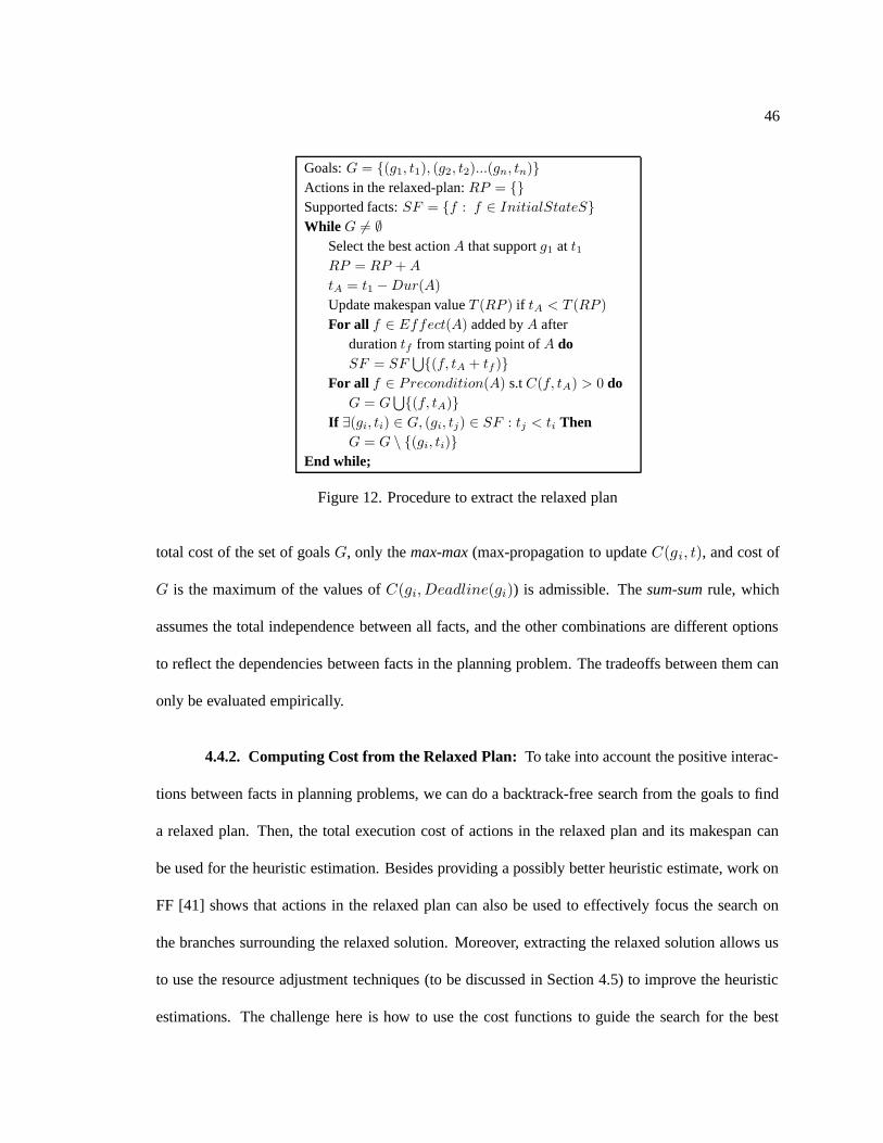
46
Goals: G = {(g1, t1), (g2, t2)...(gn, tn)}
Actions in the relaxed-plan: RP = {}
Supported facts: SF = {f : f ∈ InitialStateS}
While G 6= ∅
Select the best action A that support g1 at t1RP = RP + A
tA = t1 −Dur(A)
Update makespan value T (RP ) if tA < T (RP )
For all f ∈ Effect(A) added by A afterduration tf from starting point of A doSF = SF
⋃
{(f, tA + tf )}
For all f ∈ Precondition(A) s.t C(f, tA) > 0 doG = G
⋃
{(f, tA)}
If ∃(gi, ti) ∈ G, (gi, tj) ∈ SF : tj < ti ThenG = G \ {(gi, ti)}
End while;
Figure 12. Procedure to extract the relaxed plan
total cost of the set of goals G, only the max-max (max-propagation to update C(gi, t), and cost of
G is the maximum of the values of C(gi, Deadline(gi)) is admissible. The sum-sum rule, which
assumes the total independence between all facts, and the other combinations are different options
to reflect the dependencies between facts in the planning problem. The tradeoffs between them can
only be evaluated empirically.
4.4.2. Computing Cost from the Relaxed Plan: To take into account the positive interac-
tions between facts in planning problems, we can do a backtrack-free search from the goals to find
a relaxed plan. Then, the total execution cost of actions in the relaxed plan and its makespan can
be used for the heuristic estimation. Besides providing a possibly better heuristic estimate, work on
FF [41] shows that actions in the relaxed plan can also be used to effectively focus the search on
the branches surrounding the relaxed solution. Moreover, extracting the relaxed solution allows us
to use the resource adjustment techniques (to be discussed in Section 4.5) to improve the heuristic
estimations. The challenge here is how to use the cost functions to guide the search for the best
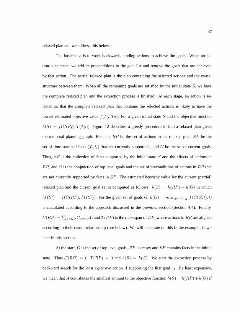
47
relaxed plan and we address this below.
The basic idea is to work backwards, finding actions to achieve the goals. When an ac-
tion is selected, we add its preconditions to the goal list and remove the goals that are achieved
by that action. The partial relaxed plan is the plan containing the selected actions and the causal
structure between them. When all the remaining goals are satisfied by the initial state S, we have
the complete relaxed plan and the extraction process is finished. At each stage, an action is se-
lected so that the complete relaxed plan that contains the selected actions is likely to have the
lowest estimated objective value f(PS , TS). For a given initial state S and the objective function
h(S) = f(C(PS), T (PS)), Figure 12 describes a greedy procedure to find a relaxed plan given
the temporal planning graph. First, let RP be the set of actions in the relaxed plan, SF be the
set of time-stamped facts (fi, ti) that are currently supported , and G be the set of current goals.
Thus, SF is the collection of facts supported by the initial state S and the effects of actions in
RP , and G is the conjunction of top level goals and the set of preconditions of actions in RP that
are not currently supported by facts in SF . The estimated heuristic value for the current (partial)
relaxed plan and the current goal set is computed as follows: h(S) = h(RP ) + h(G) in which
h(RP ) = f(C(RP ), T (RP )). For the given set of goals G, h(G) = minτ0<t<τ∞ f(C(G, t), t)
is calculated according to the approach discussed in the previous section (Section 4.4). Finally,
C(RP ) =∑
A∈RP Cexec(A) and T (RP ) is the makespan of RP , where actions in RP are aligned
according to their causal relationship (see below). We will elaborate on this in the example shown
later in this section.
At the start, G is the set of top level goals, RP is empty and SF contains facts in the initial
state. Thus C(RP ) = 0, T (RP ) = 0 and h(S) = h(G). We start the extraction process by
backward search for the least expensive action A supporting the first goal g1. By least expensive,
we mean that A contributes the smallest amount to the objective function h(S) = h(RP )+h(G) if
48
A is added to the current relaxed plan. Specifically, for each action A that supports g1, we calculate
the value hA(S) = h(RP +A)+h((G\Effect(A))⋃
Precond(A)) which estimates the heuristic
value if we add A to the relaxed plan. We then choose the action A that has the smallest hA(S)
value.
When an action A is chosen, we put its preconditions into the current goal list G, and its
effects into the set of supported facts SF . Moreover, we add a precedence constraint between A
and the action A1 that has g1 as its precondition so that A gives g1 before the time point at which A1
needs it. Using these ordering relations between actions in RP and the mutex orderings discussed
in Section 4.5, we can update the makespan value T (RP ) of the current (partial) relaxed plan.
In our ongoing example, suppose that our objective function is h(S) = f(C(PS), T (PS)) =
α.C(PS)+(1−α).T (PS ), with α = 0.55 and the infinite-lookahead criterion is used to stop the cost
propagation process. When we start extracting the relaxed plan, the initial setting is G = {at la},
RP = ∅ and SF = {at tucson}. Among the three actions Dc2t→la, Tlv→la and Fp→la that support
the goal at la, we choose action A = Fp→la because if we add it to the relaxed plan RP , then the
estimated value hA(S) = h(RP + A) + h((G \ at la)⋃
at phx) = (α ∗ Cexec(Fp→la) + (1 −
α) ∗ Dur(Fp→la)) + mint(f(C(at phx), t)) = (0.55*6.0 + 0.45*1.5) + (0.55*1.5 + 0.45*1.5) =
5.475. This turns out to be the smallest among the three actions. After we add Fp→la to the relaxed
plan, we update the goal set to G = {at phx}. It is then easy to compare between the two actions
Dc2t→phx and Dc1
t→phx to see that Dc2t→phx is cheaper for achieving at-phx given the value α = 0.55.
The final cost C(PS) = 6.0 + 1.5 = 7.5 and makespan of T (PS) = 1.5 + 1.5 = 3 of the final
relaxed plan can be used as the final heuristic estimation h(S) = 0.55 ∗ 7.5 + 0.45 ∗ 3 = 5.475 for
the given state.
Notice that in the relaxed-plan extraction procedure, we set the time points for the goal set
to be the goal deadlines, instead of the latest time points where the cost functions for the goals
49
stabilized. The reason is that the cost values of facts and actions monotonically decrease and the
costs are time-sensitive. Therefore, the later we set the time points for goals to start searching for
the relaxed plan, the better chance we have of getting the low-cost plan, especially when we use
the k-lookahead approximation approach with k 6= ∞. In our ongoing example, if we use the
zero-lookahead option to stop the propagation, we find that the smallest cost is C(in la) = 8.0 at
t = 2.5. If we search back for the relaxed plan with the combination (in la, 2.5) then we would
find a plan P1 = (Dc1t→p, Fp→la). However, if we search from the goal deadline, say t = 7.0, then
we would realize that the lowest cost for the precondition in phx of Fp→la at t = 7.0 − 1.5 = 5.5
is C(in phx, 5.5) = 1.5 (caused by Dc2t→p at time point t = 2.0) and thus the final plan is P2 =
(Dc2t→p, Fp→la) which is cheaper than P1.
4.4.3. Origin of Action Costs: In all our preceding discussion of cost-based heuristics,
we have implicitly assumed that the individual action costs are specified directly as part of the
problem specification. While this is a reasonable assumption, it can also be argued that unlike the
duration, the cost of an action is implicitly dependent on what the user is interested in optimizing.
For example, suppose, in a transportation domain, the user declares the objective function to be
optimized as:8
4 ∗ TotalT ime + 0.005 ∗ TotalFuelUsed
without providing any additional explicit information about action costs. It is possible to use the
objective function to assess the costs of individual actions (in terms of how much they contribute to
the cost portion of the objective). Specifically, the cost each action can be set equal to the amount
of fuel used by that action. The α value (for combining cost and makespan) can be set based on the
8In fact, this was the metric specified for the first problem in the Zeno-Travel domain in IPC 2003.

50
coefficients in the objective function. Of course, this type of “de-compilation” of the objective func-
tion into action costs is only possible if the objective function is a linear combination of makespan
and resource consumption.
4.5. Adjustments to the Relaxed Plan Heuristic
Until now, the heuristic estimates have been calculated by relaxing certain types of con-
straints such as negative effects and metric resource consumptions. In this section, we discuss how
those constraints can then be used to adjust and improve the final heuristic values.
4.5.1. Improving the Relaxed Plan Heuristic Estimation with Static Mutex Relations.
When building the relaxed temporal planning graph (RTPG), we ignored the negative interactions
between concurrent actions. We now discuss a way of using the static mutex relations to help im-
prove the heuristic estimation when extracting the relaxed plan. Specifically, our approach involves
the following steps:
1. Find the set of static mutex relations between the ground actions in the planning problem
based on their negative interactions.9
2. When extracting the relaxed plan, besides the orderings between actions that have causal
relationships (i.e one action gives the effect that supports the other action’s preconditions),
we also post precedence constraints to avoid concurrent execution of actions that are mutex.
Specifically, when a new action is added to the relaxed plan, we use the pre-calculated static
mutexes to establish ordering between mutually exclusive action pairs so that they can not be
executed concurrently. The orderings are selected in such a way that they violate the least
number of existing causal links in the relaxed plan.
9Two actions are static mutex if the delete effects of one action intersect with the preconditions or add effects of theother.
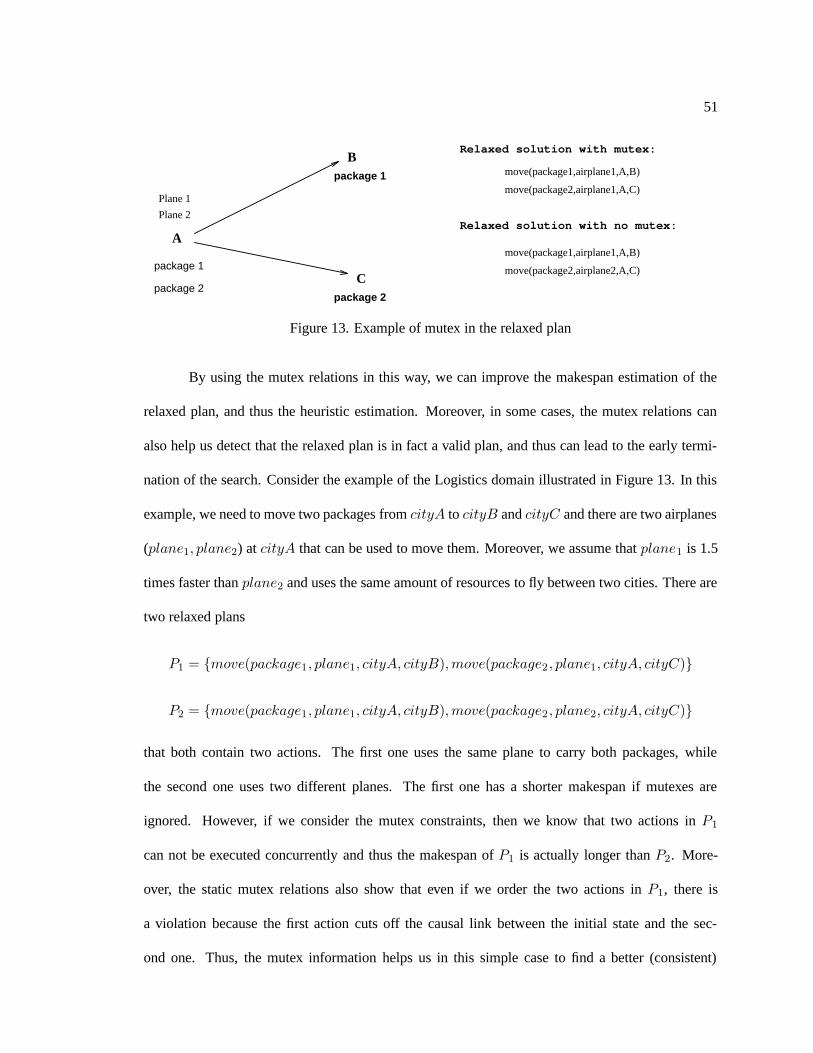
51
A
Plane 2
Plane 1
package 1
package 2
package 1
package 2
B
C
move(package1,airplane1,A,B)
move(package2,airplane1,A,C)
Relaxed solution with mutex:
move(package1,airplane1,A,B)
Relaxed solution with no mutex:
move(package2,airplane2,A,C)
Figure 13. Example of mutex in the relaxed plan
By using the mutex relations in this way, we can improve the makespan estimation of the
relaxed plan, and thus the heuristic estimation. Moreover, in some cases, the mutex relations can
also help us detect that the relaxed plan is in fact a valid plan, and thus can lead to the early termi-
nation of the search. Consider the example of the Logistics domain illustrated in Figure 13. In this
example, we need to move two packages from cityA to cityB and cityC and there are two airplanes
(plane1, plane2) at cityA that can be used to move them. Moreover, we assume that plane1 is 1.5
times faster than plane2 and uses the same amount of resources to fly between two cities. There are
two relaxed plans
P1 = {move(package1, plane1, cityA, cityB),move(package2 , plane1, cityA, cityC)}
P2 = {move(package1, plane1, cityA, cityB),move(package2 , plane2, cityA, cityC)}
that both contain two actions. The first one uses the same plane to carry both packages, while
the second one uses two different planes. The first one has a shorter makespan if mutexes are
ignored. However, if we consider the mutex constraints, then we know that two actions in P1
can not be executed concurrently and thus the makespan of P1 is actually longer than P2. More-
over, the static mutex relations also show that even if we order the two actions in P1, there is
a violation because the first action cuts off the causal link between the initial state and the sec-
ond one. Thus, the mutex information helps us in this simple case to find a better (consistent)
52
relaxed plan to use as a heuristic estimate. Here is a sketch of how the relaxed plan P2 can be
found. After the first action A1 = move(package1, plane1, cityA, cityB) is selected to support
the goal at(package1, cityB), the relaxed plan is RP = A1 and the two potential actions to sup-
port the second goal at(package2, cityC) are A2 = move(package2, plane1, cityA, cityC) and
A′2 = move(package2, plane2, cityA, cityC). With mutex information, we will be able to choose
A′2 over A2 to include in the final relaxed plan.
4.5.2. Using Resource Information to Adjust the Cost Estimates. The heuristics dis-
cussed in Section 4.4 have used the knowledge about durations of actions and deadline goals but not
resource consumption. By ignoring the resource related effects when building the relaxed plan, we
may miss counting actions whose only purpose is to provide sufficient resource-related conditions
to other actions. In our ongoing example, if we want to drive a car from Tucson to LA and the gas
level is low, by totally ignoring the resource related conditions, we will not realize that we need to
refuel the car before drive. Consequently, ignoring resource constraints may reduce the quality of
the heuristic estimate based on the relaxed plan. We are thus interested in adjusting the heuristic
values discussed in the last two sections to account for the resource constraints.
In many real-world problems, most actions consume resources, while there are special ac-
tions that increase the levels of resources. Since checking whether the level of a resource is sufficient
for allowing the execution of an action is similar to checking the predicate preconditions, one ob-
vious approach is to adjust the relaxed plan by including actions that provide that resource-related
condition to the relaxed plan. However, for many reasons, it turns out to be too difficult to decide
which actions should be added to the relaxed plan to satisfy the given resource conditions (In [19],
we give a more detailed discussion of these difficulties). Therefore, we introduce an indirect way
of adjusting the cost of the relaxed plan to take into account the resource constraints. We first pre-
53
process the problem specifications and find for each resource R an action AR that can increase the
amount of R maximally. Let ∆R be the amount by which AR increases R, and let C(AR) be the cost
value of AR. Let Init(R) be the level of resource R at the state S for which we want to compute
the relaxed plan, and Con(R), Pro(R) be the total consumption and production of R by all actions
in the relaxed plan. If Con(R) > Init(R) + Pro(R), then we increase the cost by the number of
production actions necessary to make up the difference. More precisely:
C ← C +∑
R
⌈
(Con(R)− (Init(R) + Pro(R)))
∆R
⌉
∗ C(AR)
We shall call this the adjusted cost heuristic. The basic idea is that even though we do
not know if an individual resource-consuming action in the relaxed plan needs another action to
support its resource-related preconditions, we can still adjust the number of actions in the relaxed
plan by reasoning about the total resource consumption of all the actions in the plan. If we know
the resources R consumed by the relaxed plan and the maximum production of those resources
possible by any individual action in the domain, then we can infer the minimum number of resource-
increasing actions that we need to add to the relaxed plan to balance the resource consumption. In
our ongoing example, if the car rented by the students at Tucson does not have enough fuel in the
initial state to make the trip to Phoenix, LA, or Las Vegas, then this approach will discover that the
planner needs to add a refuel action to the relaxed plan.
Currently, our resource-adjustment technique discussed above is limited to simple consump-
tion and production of resources using addition and subtraction. These are the most common forms,
as evidenced by the fact that in all metric temporal planning domains used in the competition, ac-
tions consume and produce resources solely using addition (increase) and subtraction (decrease).
Modifications are needed to extend our current approach to deal with other types of resource con-
sumption such as using multiplication or division.
54
4.6. Summary and Discussion
In this chapter, we discuss the issue of deriving heuristics, which are sensitive to both time
and cost, from the temporal planning graph. We also introduce an approach of tracking costs of
achieving goals and other facts as functions of time to guide the multi-objective search. We plan on
extending and improving this current multi-objective heuristic search framework in several direc-
tions:
Multi-Objective Search: While we considered cost of a plan in terms of a single monetary cost
associated with each action, in more complex domains, the cost may be better defined as a vector
comprising different types of resource consumption. Further, in addition to cost and makespan, we
may also be interested in other measures of plan quality such as robustness and execution flexibility
of the plan. To this end, we plan to extend our methodology to derive heuristics sensitive to a larger
variety of quality measures. Besides heuristic estimates, we also intend to investigate different
multi-objective search frameworks such as priotizing different criteria or pareto-set optimization. In
multi-objective planning scenario, it’s important to have the ability to find a decent quality plan and
later improve it as given more time or finding multiple non-dominated plans. In this sense, work
in anytime search algorithm for Sapaps in Chapter 7, which gradually returns better quality plans
given a single objective function, can help in multi-objective search.
Heuristic and Scalability: In our current framework of propagating the cost functions over the
planning graph, while the cost estimation using relaxed-plan extraction over the cost functions
seems to be reasonably good heuristic, the time-estimation using the first time point at which the
goal appears in the relaxed planning graph seems to underestimate the real time needed to achieve
that given goal. The evidence is that TGP and TP4 perform much better than Sapa using this heuris-
tic for finding optimal makespan plan. Because time-related plan qualities are important and we are
55
also looking at extending the Sapa and Sapaps planners to deal with more plan metrics depending
on time, improving goal achievement and action starting time estimation over the planning graph is
an important issue. One option would be to use the mutex relations more aggressively. Neverthe-
less, due to the current framework of having to build a separated planning graph for each generated
state, the traditional approach of mutex propagation seems to be too costly. One cheaper alternative
would be to use only pre-collected static mutexes when building the planning graph but ignore the
dynamic propagation. However, this approach still suffers from having to explicitly reason about
mutex relations between every pair of facts and actions at each (important) time point. Currently,
we believe that the best approach would be to use the pre-processing tool such as the one used in
the “fast-downward” planner [40] to convert PDDL into the multi-valued SAS+ representation. The
mutex relations are implicitly embedded in different values of the same variable and thus we do not
need to explicitly reason about them when building the graph10 . Besides heuristic quality, we also
plan on improving the time to extract the heuristic by exploiting ways to reuse the planning graph
between related search nodes. This approach was used in the Optop planner [64], which also does
forward search. However, keeping the planning graph for every search node with hope to use it later
(if that node is selected) may be too expensive in terms of memory usage. Therefore, we plan to use
it only for (enforced) “hill-climbing” style search where all search nodes belong to one branch from
the root node and thus consecutively explored nodes are similar to each other (which maximize the
possibility of reusing most of the previous planning graph).
Exogenous event, in the name of timed-initial-literal, is one of two recent important ex-
tensions to PDDL2.1 planning language (along with domain axiom). In the previous chapter, we
discussed how exogenous events can be handled in the current forward search framework of Sapa
by representing them as events in the event queue of the initial state. In fact, Sapa can solve the
10The other advantage of this approach is the reduced set of variables which can lead to a significantly smaller graphstructure
56
sample problem involving timed-initial-literal in the IPC4 in a quite short time. Even though ex-
tending the search framework to take exogenous event into account is easy, modifying the heuristic
estimation process to adapt to the additional constraints caused by exogenous events is not easy.
On one hand, exogenous events appear like normal instantaneous actions occurring at fixed time-
points; on the other hand, they are different from normal actions in the sense that planners can not
choose whether or not to include them in the final plan. Therefore, in the current planning graph
building process, even though normal actions are put in even when there are mutex relations with
other actions at the same time point (because there is no guarantee that the mutexed actions would
be selected in the final plan), treating exogenous events the same way would lower the heuristic
quality. This is because exogenous events are guaranteed to be in any valid plan and thus any action
that conflicts with any of the exogenous events would definitely not be in the final plan. Given
this observation, we are investigating several modifications to the current planning graph building
process when there exist exogenous events. They are: (i) an approach to de-activate (remove) ac-
tions from the planning graph if their preconditions are no longer hold true due to the conflicts with
exogenous events; (ii) a technique of maitaining multiple noop actions with different costs; and (iii)
maintaining non-monotonic cost functions for facts and actions affected by exogenous events.
For the cost estimation in the current framework, even though the sum-propagation rule
tends to over-estimate the achievement cost badly, the later phase of relaxed plan extraction tends
to correct this and give good estimation in term of total planning cost. However, the relaxed-plan
extraction phase is still dependent on the propagated cost function. Therefore, improvement in the
cost-propagation phase can potentially improve the overall heuristic quality. Currently, we are im-
plementing a new “union” propagation rule that take into account the duplications in the “max”
propagation rule and thus improve the quality of the cost function11 . More specifically, while con-
11This technique was hinted by David Smith at the proposal defense time.

57
ducting cost-propagation, for each fact, we keep a estimated lowest total cost set of actions (equals
to a relaxed plan) that supports each fact. The estimated cost to execute an action is then calcu-
lated by taking the total cost of the union of action sets that supporting its preconditions. This is
potentially a better estimation than simply taking the sum or max of the values to support individual
preconditions.
Some of the resource and temporal constraints (e.g. exogenous events, discrete resources)
has been extensively investigated in the scheduling community. Therefore, we plan to look at: (i)
how to use scheduling techniques to improve the heuristic quality to guide the metric temporal plan-
ner; and (ii) an effective framework to separate the set of logical, temporal, and resource constraints
between two different modules: a planner and a scheduler. For the first direction, our preliminary
investigation in [23] is a starting point in integrating scheduling techniques into metric temporal
planning. For the second direction, our previous work in the RealPlan system [86] showed that in
many planning scenarios, decoupling and integrating a planner and scheduler can significantly scale
up the overall system’s performance. Nevertheless, RealPlan was designed for classical scenario so
extending the framework to metric temporal planning is very promising.
CHAPTER 5
Implementation & Empirical Evaluation
The Sapa system with all the techniques described in this paper has been implemented in
Java. The implementation includes:
1. The forward chaining algorithm (Section 3).
2. The cost sensitive temporal planning graph and the routines to propagate the cost information
and extract the heuristic value from it (Section 4.1 and 4.2).
3. The routines to extract and adjust the relaxed plan using static mutex and resource information
(Section 4.4).
By default Sapa uses the sum-propagation rule, infinite lookahead termination, resource-
adjusted heuristics, and converts the solutions into o.c. plans. Besides the techniques described in
this paper, we also wrote a JAVA-based parser for PDDL2.1 Level 3, which is the highest level used
in the Third International Planning Competition (IPC3).
To visualize the plans returned by Sapa and the relations between actions in the plan (such
as causal links, mutual exclusions, and resource relations), we have developed a Graphical User
Interface (GUI)1 for Sapa. Figure 14 and 15 shows the screen shots of the current GUI. It displays
the time line of the final plan with each action shown with its actual duration and starting time in the
1The GUI was developed by Dan Bryce
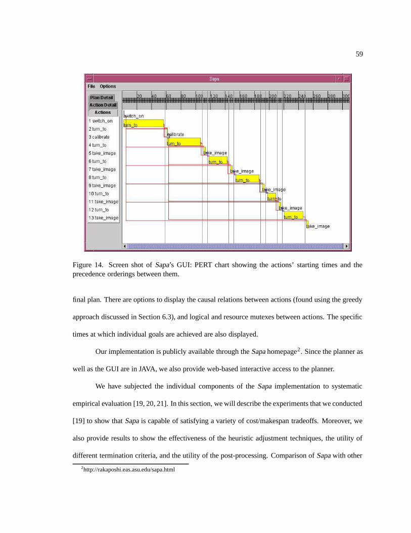
59
Figure 14. Screen shot of Sapa’s GUI: PERT chart showing the actions’ starting times and theprecedence orderings between them.
final plan. There are options to display the causal relations between actions (found using the greedy
approach discussed in Section 6.3), and logical and resource mutexes between actions. The specific
times at which individual goals are achieved are also displayed.
Our implementation is publicly available through the Sapa homepage2 . Since the planner as
well as the GUI are in JAVA, we also provide web-based interactive access to the planner.
We have subjected the individual components of the Sapa implementation to systematic
empirical evaluation [19, 20, 21]. In this section, we will describe the experiments that we conducted
[19] to show that Sapa is capable of satisfying a variety of cost/makespan tradeoffs. Moreover, we
also provide results to show the effectiveness of the heuristic adjustment techniques, the utility of
different termination criteria, and the utility of the post-processing. Comparison of Sapa with other
2http://rakaposhi.eas.asu.edu/sapa.html
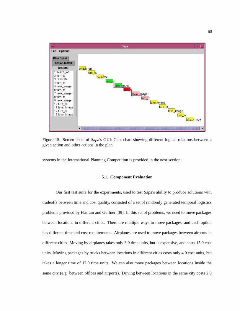
60
Figure 15. Screen shots of Sapa’s GUI: Gant chart showing different logical relations between agiven action and other actions in the plan.
systems in the International Planning Competition is provided in the next section.
5.1. Component Evaluation
Our first test suite for the experiments, used to test Sapa’s ability to produce solutions with
tradeoffs between time and cost quality, consisted of a set of randomly generated temporal logistics
problems provided by Haslum and Geffner [39]. In this set of problems, we need to move packages
between locations in different cities. There are multiple ways to move packages, and each option
has different time and cost requirements. Airplanes are used to move packages between airports in
different cities. Moving by airplanes takes only 3.0 time units, but is expensive, and costs 15.0 cost
units. Moving packages by trucks between locations in different cities costs only 4.0 cost units, but
takes a longer time of 12.0 time units. We can also move packages between locations inside the
same city (e.g. between offices and airports). Driving between locations in the same city costs 2.0
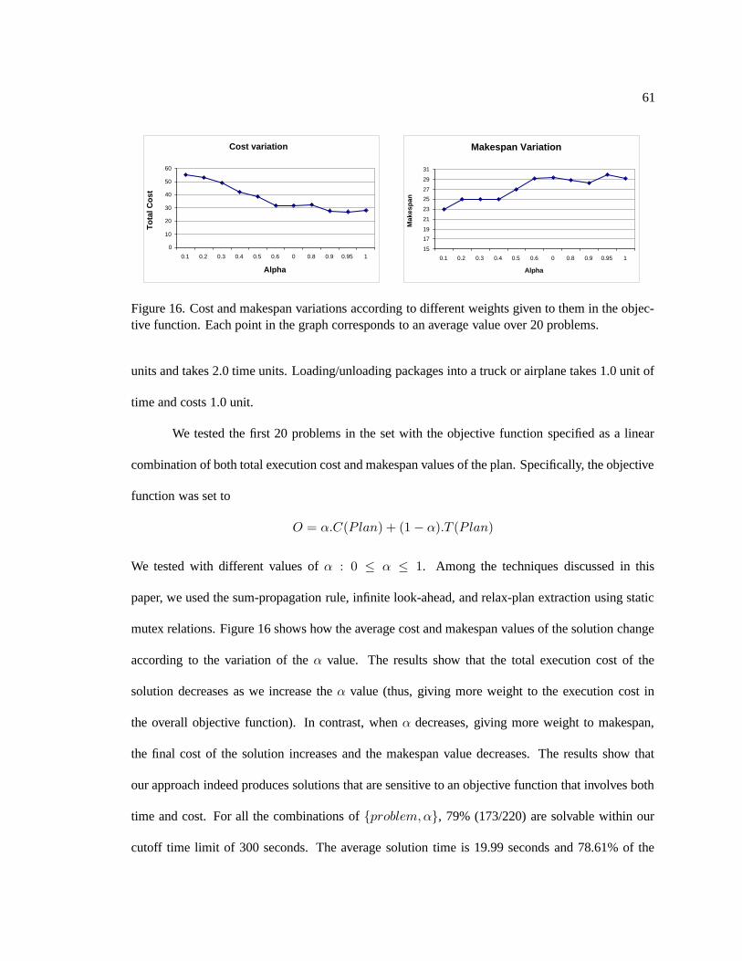
61
Cost variation
0
10
20
30
40
50
60
0.1 0.2 0.3 0.4 0.5 0.6 0 0.8 0.9 0.95 1
Alpha
To
tal C
ost
Makespan Variation
15
17
19
21
23
25
27
29
31
0.1 0.2 0.3 0.4 0.5 0.6 0 0.8 0.9 0.95 1
Alpha
Mak
esp
an
Figure 16. Cost and makespan variations according to different weights given to them in the objec-tive function. Each point in the graph corresponds to an average value over 20 problems.
units and takes 2.0 time units. Loading/unloading packages into a truck or airplane takes 1.0 unit of
time and costs 1.0 unit.
We tested the first 20 problems in the set with the objective function specified as a linear
combination of both total execution cost and makespan values of the plan. Specifically, the objective
function was set to
O = α.C(P lan) + (1− α).T (P lan)
We tested with different values of α : 0 ≤ α ≤ 1. Among the techniques discussed in this
paper, we used the sum-propagation rule, infinite look-ahead, and relax-plan extraction using static
mutex relations. Figure 16 shows how the average cost and makespan values of the solution change
according to the variation of the α value. The results show that the total execution cost of the
solution decreases as we increase the α value (thus, giving more weight to the execution cost in
the overall objective function). In contrast, when α decreases, giving more weight to makespan,
the final cost of the solution increases and the makespan value decreases. The results show that
our approach indeed produces solutions that are sensitive to an objective function that involves both
time and cost. For all the combinations of {problem, α}, 79% (173/220) are solvable within our
cutoff time limit of 300 seconds. The average solution time is 19.99 seconds and 78.61% of the
62
instances can be solved within 10 seconds.
Evaluation of Different Termination Criteria: Figure 17 shows the comparison results for zero,
one, and infinite lookahead for the set of metric temporal planning problems in the competition.
We take the first 12 problems in each of the four temporal domains: ZenoTravel-Time, DriverLog-
Time, Satellite-Time, and RoversTime. We set α = 1 in the objective function, making it entirely
cost-based. The action costs are set to 1 unit. As discussed in Section 4.3, zero-lookahead stops the
cost propagation process at the time point where there is a solution under the relaxed condition. K-
lookahead spends extra effort to go beyond that time point in hope of finding better quality (relaxed)
solution to use as heuristic values to guide the search. The running condition is specified in the
caption of the figure.
For most of the problems in the three domains ZenoTravel-Time, DriverLog-Time,
and Satellite-Time, infinite-lookahead returns better quality solutions in shorter time than one-
lookahead, which in turn is generally better than zero-lookahead. The exception is the Rovers-Time
domain, in which there is virtually no difference in running time or solution quality between the
different look-ahead options.
The following is a more elaborate summary of the results in Figure 17. The top three figures
show the running time, cost, and makespan comparisons in the ZenoTravel domain (Time setting).
In this domain, within the time and memory limit, infinite-lookahead helps to solve 3 more problems
than one-lookahead and 2 more than zero-lookahead. In all but one problem (problem 10), infinite-
lookahead returns equal (three) or better (eight) cost solution than zero-lookahead. Compared to
one-lookahead, it’s better in five problems and equal in six others. For the makespan value, infinite-
lookahead is generally better, but not as consistent as other criteria. The next three lower figures
show the comparison results for the DriverLog-Time domain. In this domain, infinite and one-
lookahead solve one more problem than zero-lookahead, infinite-lookahead is also faster than the
63
other two options in all but one problem. The costs (number of actions) of solutions returned by
infinite-lookahead are also better than all but two of the problems (in which all three solutions are the
same). One-lookahead is also equal to or better than zero-lookahead in all but two problems. In the
Satellite-Time domain, while infinite and one-lookahead solve three more (of twelve) problems than
zero-lookahead, there is no option that consistently solves problems faster than the other. However,
the solution quality (cost) of infinite and one-lookahead is consistently better than zero-lookahead.
Moreover, the solution cost of plans returned by infinite-lookahead is worse than one-lookahead in
only one problem while being slightly better in 6 problems. In this domain, it seems that there is big
improvement from zero to one look-ahead, while infinite-lookahead is a slight improvement over
one-lookahead. (The plots for the Rovers domain are not shown in the figure as all the different
look-ahead options seem to lead to near identical results in that domain.) Finally, since the heuristic
is based completely on cost (α =1), we do not, in theory, expect to see any conclusive patterns in
the makespan values of the solutions produced for the different lookahead options.
Utility of the Resource Adjustment Technique: In our previous work [19], we show that the
resource adjustment technique can lead to significant quality and search speed improvements in
problems such as the metric temporal logistics domain in which there are several types of resource
consumption objects like trucks and airplanes.
In the competition, there are two domains in which we can test the utility of the resource
adjustment technique discussed in Section 4.5. The ZenoTravel domain and the Rovers domain
have actions consuming resources and other (refueling) actions to renew them. Of these, the re-
source adjustment technique gives mixed results in the ZenoTravel domain and has no effect in
the Rovers domain. Therefore, we only show the comparison for the ZenoTravel domain in Fig-
ure 18. In the ZenoTravel domain, Sapa with the resource adjustment runs slightly faster in 10 of 14
problems, returns shorter solutions in 5 problems and longer solutions in 3 problems. The solution
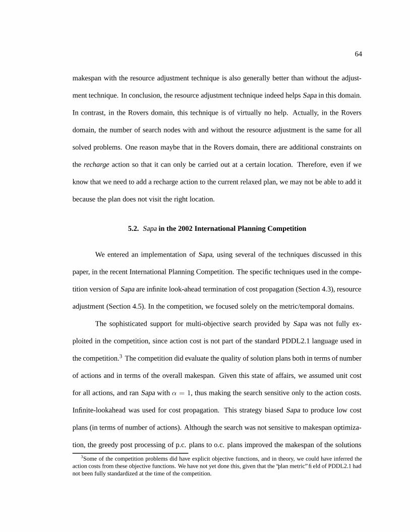
64
makespan with the resource adjustment technique is also generally better than without the adjust-
ment technique. In conclusion, the resource adjustment technique indeed helps Sapa in this domain.
In contrast, in the Rovers domain, this technique is of virtually no help. Actually, in the Rovers
domain, the number of search nodes with and without the resource adjustment is the same for all
solved problems. One reason maybe that in the Rovers domain, there are additional constraints on
the recharge action so that it can only be carried out at a certain location. Therefore, even if we
know that we need to add a recharge action to the current relaxed plan, we may not be able to add it
because the plan does not visit the right location.
5.2. Sapa in the 2002 International Planning Competition
We entered an implementation of Sapa, using several of the techniques discussed in this
paper, in the recent International Planning Competition. The specific techniques used in the compe-
tition version of Sapa are infinite look-ahead termination of cost propagation (Section 4.3), resource
adjustment (Section 4.5). In the competition, we focused solely on the metric/temporal domains.
The sophisticated support for multi-objective search provided by Sapa was not fully ex-
ploited in the competition, since action cost is not part of the standard PDDL2.1 language used in
the competition.3 The competition did evaluate the quality of solution plans both in terms of number
of actions and in terms of the overall makespan. Given this state of affairs, we assumed unit cost
for all actions, and ran Sapa with α = 1, thus making the search sensitive only to the action costs.
Infinite-lookahead was used for cost propagation. This strategy biased Sapa to produce low cost
plans (in terms of number of actions). Although the search was not sensitive to makespan optimiza-
tion, the greedy post processing of p.c. plans to o.c. plans improved the makespan of the solutions
3Some of the competition problems did have explicit objective functions, and in theory, we could have inferred theaction costs from these objective functions. We have not yet done this, given that the “plan metric” field of PDDL2.1 hadnot been fully standardized at the time of the competition.
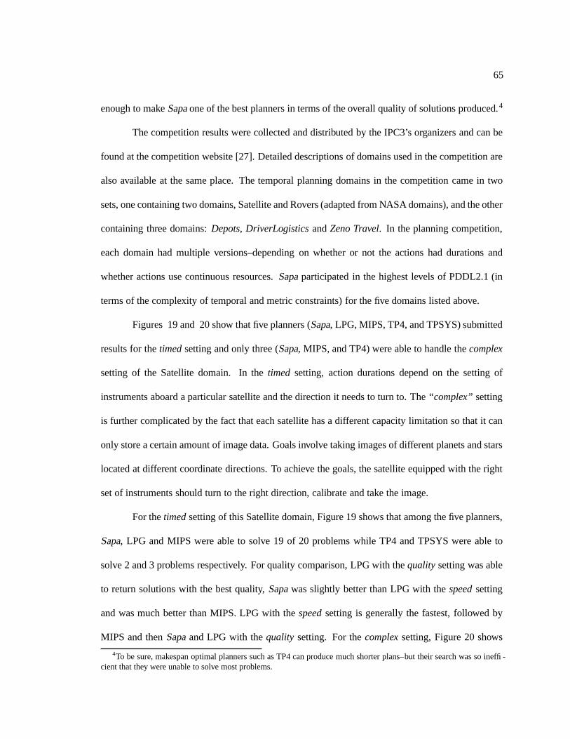
65
enough to make Sapa one of the best planners in terms of the overall quality of solutions produced.4
The competition results were collected and distributed by the IPC3’s organizers and can be
found at the competition website [27]. Detailed descriptions of domains used in the competition are
also available at the same place. The temporal planning domains in the competition came in two
sets, one containing two domains, Satellite and Rovers (adapted from NASA domains), and the other
containing three domains: Depots, DriverLogistics and Zeno Travel. In the planning competition,
each domain had multiple versions–depending on whether or not the actions had durations and
whether actions use continuous resources. Sapa participated in the highest levels of PDDL2.1 (in
terms of the complexity of temporal and metric constraints) for the five domains listed above.
Figures 19 and 20 show that five planners (Sapa, LPG, MIPS, TP4, and TPSYS) submitted
results for the timed setting and only three (Sapa, MIPS, and TP4) were able to handle the complex
setting of the Satellite domain. In the timed setting, action durations depend on the setting of
instruments aboard a particular satellite and the direction it needs to turn to. The “complex” setting
is further complicated by the fact that each satellite has a different capacity limitation so that it can
only store a certain amount of image data. Goals involve taking images of different planets and stars
located at different coordinate directions. To achieve the goals, the satellite equipped with the right
set of instruments should turn to the right direction, calibrate and take the image.
For the timed setting of this Satellite domain, Figure 19 shows that among the five planners,
Sapa, LPG and MIPS were able to solve 19 of 20 problems while TP4 and TPSYS were able to
solve 2 and 3 problems respectively. For quality comparison, LPG with the quality setting was able
to return solutions with the best quality, Sapa was slightly better than LPG with the speed setting
and was much better than MIPS. LPG with the speed setting is generally the fastest, followed by
MIPS and then Sapa and LPG with the quality setting. For the complex setting, Figure 20 shows
4To be sure, makespan optimal planners such as TP4 can produce much shorter plans–but their search was so ineffi-cient that they were unable to solve most problems.
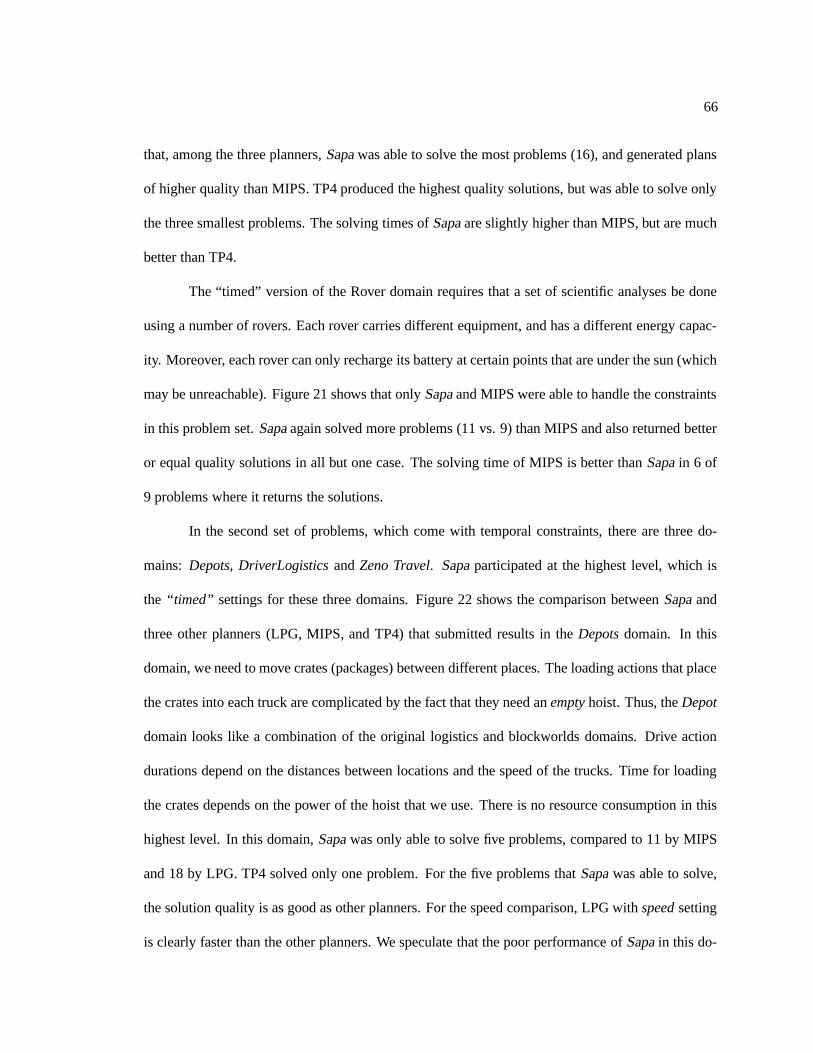
66
that, among the three planners, Sapa was able to solve the most problems (16), and generated plans
of higher quality than MIPS. TP4 produced the highest quality solutions, but was able to solve only
the three smallest problems. The solving times of Sapa are slightly higher than MIPS, but are much
better than TP4.
The “timed” version of the Rover domain requires that a set of scientific analyses be done
using a number of rovers. Each rover carries different equipment, and has a different energy capac-
ity. Moreover, each rover can only recharge its battery at certain points that are under the sun (which
may be unreachable). Figure 21 shows that only Sapa and MIPS were able to handle the constraints
in this problem set. Sapa again solved more problems (11 vs. 9) than MIPS and also returned better
or equal quality solutions in all but one case. The solving time of MIPS is better than Sapa in 6 of
9 problems where it returns the solutions.
In the second set of problems, which come with temporal constraints, there are three do-
mains: Depots, DriverLogistics and Zeno Travel. Sapa participated at the highest level, which is
the “timed” settings for these three domains. Figure 22 shows the comparison between Sapa and
three other planners (LPG, MIPS, and TP4) that submitted results in the Depots domain. In this
domain, we need to move crates (packages) between different places. The loading actions that place
the crates into each truck are complicated by the fact that they need an empty hoist. Thus, the Depot
domain looks like a combination of the original logistics and blockworlds domains. Drive action
durations depend on the distances between locations and the speed of the trucks. Time for loading
the crates depends on the power of the hoist that we use. There is no resource consumption in this
highest level. In this domain, Sapa was only able to solve five problems, compared to 11 by MIPS
and 18 by LPG. TP4 solved only one problem. For the five problems that Sapa was able to solve,
the solution quality is as good as other planners. For the speed comparison, LPG with speed setting
is clearly faster than the other planners. We speculate that the poor performance of Sapa in this do-
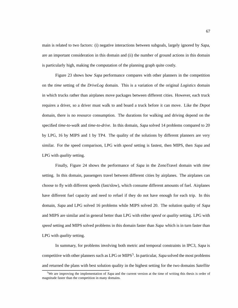
67
main is related to two factors: (i) negative interactions between subgoals, largely ignored by Sapa,
are an important consideration in this domain and (ii) the number of ground actions in this domain
is particularly high, making the computation of the planning graph quite costly.
Figure 23 shows how Sapa performance compares with other planners in the competition
on the time setting of the DriveLog domain. This is a variation of the original Logistics domain
in which trucks rather than airplanes move packages between different cities. However, each truck
requires a driver, so a driver must walk to and board a truck before it can move. Like the Depot
domain, there is no resource consumption. The durations for walking and driving depend on the
specified time-to-walk and time-to-drive. In this domain, Sapa solved 14 problems compared to 20
by LPG, 16 by MIPS and 1 by TP4. The quality of the solutions by different planners are very
similar. For the speed comparison, LPG with speed setting is fastest, then MIPS, then Sapa and
LPG with quality setting.
Finally, Figure 24 shows the performance of Sapa in the ZenoTravel domain with time
setting. In this domain, passengers travel between different cities by airplanes. The airplanes can
choose to fly with different speeds (fast/slow), which consume different amounts of fuel. Airplanes
have different fuel capacity and need to refuel if they do not have enough for each trip. In this
domain, Sapa and LPG solved 16 problems while MIPS solved 20. The solution quality of Sapa
and MIPS are similar and in general better than LPG with either speed or quality setting. LPG with
speed setting and MIPS solved problems in this domain faster than Sapa which is in turn faster than
LPG with quality setting.
In summary, for problems involving both metric and temporal constraints in IPC3, Sapa is
competitive with other planners such as LPG or MIPS5. In particular, Sapa solved the most problems
and returned the plans with best solution quality in the highest setting for the two domains Satellite
5We are improving the implementation of Sapa and the current version at the time of writing this thesis is order ofmagnitude faster than the competition in many domains.

68
and Rovers, which are adapted from NASA domains. A more detailed analysis of the competition
results is presented by [62].
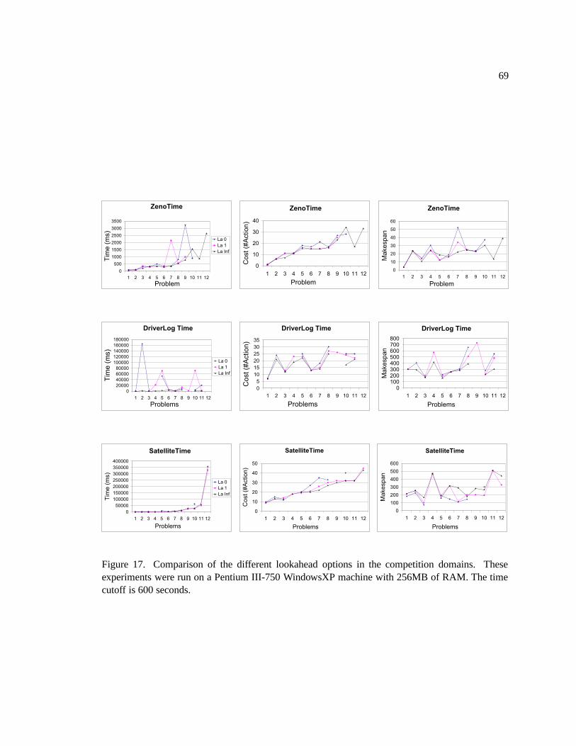
69
ZenoTime
0
500
1000
1500
2000
2500
3000
3500
1 2 3 4 5 6 7 8 9 10 11 12
Problem
Tim
e (
ms)
La 0
La 1
La Inf
ZenoTime
0
10
20
30
40
1 2 3 4 5 6 7 8 9 10 11 12
Problem
Cost (#
Action)
ZenoTime
0
10
20
30
40
50
60
1 2 3 4 5 6 7 8 9 10 11 12
Problem
Makespan
DriverLog Time
0
20000
40000
60000
80000
100000
120000
140000
160000
180000
1 2 3 4 5 6 7 8 9 10 11 12
Problems
Tim
e (
ms)
La 0
La 1
La Inf
DriverLog Time
0
5
10
15
20
25
30
35
1 2 3 4 5 6 7 8 9 10 11 12
Problems
Cost (#
Action)
DriverLog Time
0100200300400500600700800
1 2 3 4 5 6 7 8 9 10 11 12
Problems
Makespan
SatelliteTime
0
50000
100000
150000
200000
250000
300000
350000
400000
1 2 3 4 5 6 7 8 9 10 11 12
Problems
Tim
e (
ms)
La 0
La 1
La Inf
SatelliteTime
0
10
20
30
40
50
1 2 3 4 5 6 7 8 9 10 11 12
Problems
Cost
(#A
ction)
SatelliteTime
0
100
200
300
400
500
600
1 2 3 4 5 6 7 8 9 10 11 12
Problems
Makespan
Figure 17. Comparison of the different lookahead options in the competition domains. Theseexperiments were run on a Pentium III-750 WindowsXP machine with 256MB of RAM. The timecutoff is 600 seconds.
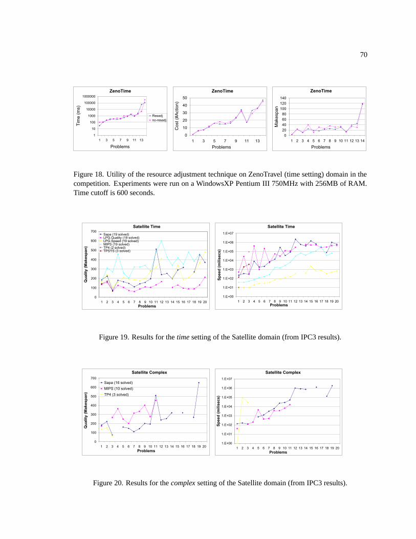
70
ZenoTime
1
10
100
1000
10000
100000
1000000
1 3 5 7 9 11 13
Problems
Tim
e (
ms)
Resadj
no-resadj
ZenoTime
0
10
20
30
40
50
1 3 5 7 9 11 13
Problems
Cost
(#A
ction)
ZenoTime
0
20
40
60
80
100
120
140
1 2 3 4 5 6 7 8 9 10 11 12 13 14
Problems
Makespan
Figure 18. Utility of the resource adjustment technique on ZenoTravel (time setting) domain in thecompetition. Experiments were run on a WindowsXP Pentium III 750MHz with 256MB of RAM.Time cutoff is 600 seconds.
Satellite Time
0
100
200
300
400
500
600
700
1 2 3 4 5 6 7 8 9 10 11 12 13 14 15 16 17 18 19 20
Problems
Qu
ali
ty (
Ma
ke
sp
an
)
Sapa (19 solved)LPG.Quality (19 solved)LPG.Speed (19 solved)MIPS (19 solved)TP4 (2 solved)TPSYS (3 solved)
Satellite Time
1.E+00
1.E+01
1.E+02
1.E+03
1.E+04
1.E+05
1.E+06
1.E+07
1 2 3 4 5 6 7 8 9 10 11 12 13 14 15 16 17 18 19 20
Problems
Sp
ee
d (
mil
ise
cs
)
Figure 19. Results for the time setting of the Satellite domain (from IPC3 results).
Satellite Complex
0
100
200
300
400
500
600
700
1 2 3 4 5 6 7 8 9 10 11 12 13 14 15 16 17 18 19 20
Problems
Qu
ali
ty (
Ma
ke
sp
an
)
Sapa (16 solved)
MIPS (10 solved)
TP4 (3 solved)
Satellite Complex
1.E+00
1.E+01
1.E+02
1.E+03
1.E+04
1.E+05
1.E+06
1.E+07
1 2 3 4 5 6 7 8 9 10 11 12 13 14 15 16 17 18 19 20
Problems
Sp
eed
(m
ilis
ecs)
Figure 20. Results for the complex setting of the Satellite domain (from IPC3 results).
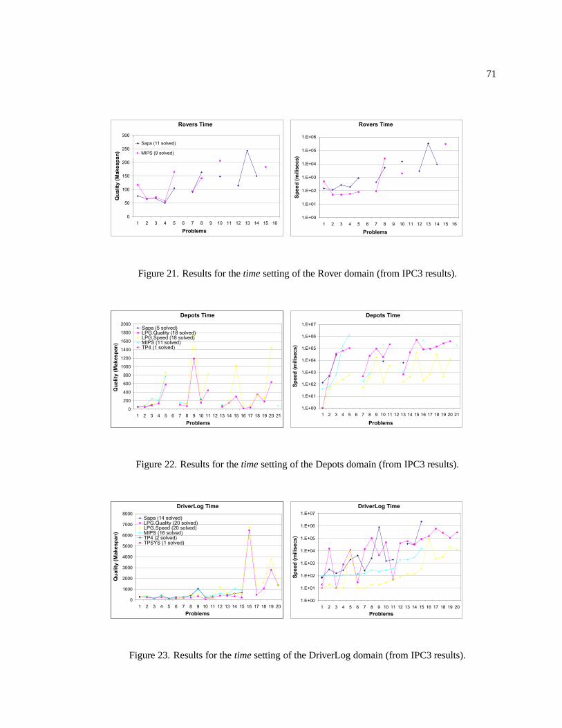
71
Rovers Time
0
50
100
150
200
250
300
1 2 3 4 5 6 7 8 9 10 11 12 13 14 15 16
Problems
Qu
ali
ty (
Ma
ke
sp
an
)
Sapa (11 solved)
MIPS (9 solved)
Rovers Time
1.E+00
1.E+01
1.E+02
1.E+03
1.E+04
1.E+05
1.E+06
1 2 3 4 5 6 7 8 9 10 11 12 13 14 15 16
Problems
Sp
ee
d (
mil
ise
cs
)
Figure 21. Results for the time setting of the Rover domain (from IPC3 results).
Depots Time
0
200
400
600
800
1000
1200
1400
1600
1800
2000
1 2 3 4 5 6 7 8 9 10 11 12 13 14 15 16 17 18 19 20 21
Problems
Qu
ality
(M
akesp
an
)
Sapa (5 solved)LPG.Quality (18 solved)LPG.Speed (18 solved)MIPS (11 solved)TP4 (1 solved)
Depots Time
1.E+00
1.E+01
1.E+02
1.E+03
1.E+04
1.E+05
1.E+06
1.E+07
1 2 3 4 5 6 7 8 9 10 11 12 13 14 15 16 17 18 19 20 21
Problems
Sp
ee
d (
mil
ise
cs
)
Figure 22. Results for the time setting of the Depots domain (from IPC3 results).
DriverLog Time
0
1000
2000
3000
4000
5000
6000
7000
8000
1 2 3 4 5 6 7 8 9 10 11 12 13 14 15 16 17 18 19 20
Problems
Qu
ali
ty (
Ma
ke
sp
an
)
Sapa (14 solved)LPG.Quality (20 solved)LPG.Speed (20 solved)MIPS (16 solved)TP4 (2 solved)TPSYS (1 solved)
DriverLog Time
1.E+00
1.E+01
1.E+02
1.E+03
1.E+04
1.E+05
1.E+06
1.E+07
1 2 3 4 5 6 7 8 9 10 11 12 13 14 15 16 17 18 19 20
Problems
Sp
ee
d (
mil
ise
cs
)
Figure 23. Results for the time setting of the DriverLog domain (from IPC3 results).
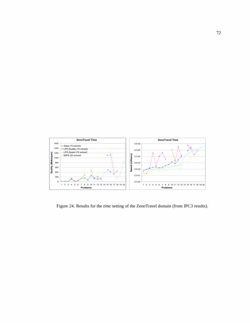
72
ZenoTravel Time
0
200
400
600
800
1000
1200
1400
1600
1 2 3 4 5 6 7 8 9 10 11 12 13 14 15 16 17 18 19 20
Problems
Qu
ali
ty (
Ma
ke
sp
an
)
Sapa (15 solved)
LPG.Quality (16 solved)
LPG.Speed (16 solved)
MIPS (20 solved)
ZenoTravel Time
1.E+00
1.E+01
1.E+02
1.E+03
1.E+04
1.E+05
1.E+06
1 2 3 4 5 6 7 8 9 10 11 12 13 14 15 16 17 18 19 20
Problems
Sp
eed
(m
ilis
ecs)
Figure 24. Results for the time setting of the ZenoTravel domain (from IPC3 results).
CHAPTER 6
Improving Solution Quality by Partialization
As mentioned in Chapter 2 on background on planning, plans can be classified broadly into
two categories–“position constrained” (p.c.) and “order constrained” (o.c.). The former specifies
the exact start time for each of the actions in the plan, while the latter only specifies the relative
orderings between different actions (Figure 25 shows the examples of these two types of plans).
The two types of plans offer complementary tradeoffs vis a vis search and execution. Specifically,
constraining the positions gives complete state information about the partial plan, making it easier
to control the search (viz., it is easy to compute the resource levels and check for the consistency of
temporal constraints at every point in a partial plan). Not surprisingly, several of the more effective
methods for plan synthesis in metric temporal domains search for and generate p.c. plans (c.f.
TLPlan[1], Sapa[19], TGP [81], MIPS[24]). Position constrained plans are however less desirable
from the point of view of execution flexibility and human comprehension (e.g. no causal relations
between actions in the plan are shown). At the same time, from an execution point of view, o.c.
plans are more advantageous than p.c. plans –they provide better execution flexibility both in terms
of makespan and in terms of “scheduling flexibility” (which measures the possible execution traces
supported by the plan [87, 71]). They are also more effective in interfacing the planner to other
modules such as schedulers (c.f. [86, 59]), and in supporting replanning and plan reuse [90, 45].1
1Precedence constrained plan or order constrained plan (o.c plan) is also the preferred choice for lifted planning.
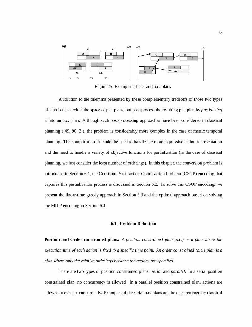
74
T4 T2T3 T1
{Q} {G} {Q} {G}
RQ
S~R
RS
RG
A4:A3:
A1: A2:
QR
~RS
SR
RG
Figure 25. Examples of p.c. and o.c. plans
A solution to the dilemma presented by these complementary tradeoffs of those two types
of plan is to search in the space of p.c. plans, but post-process the resulting p.c. plan by partializing
it into an o.c. plan. Although such post-processing approaches have been considered in classical
planning ([49, 90, 2]), the problem is considerably more complex in the case of metric temporal
planning. The complications include the need to handle the more expressive action representation
and the need to handle a variety of objective functions for partialization (in the case of classical
planning, we just consider the least number of orderings). In this chapter, the conversion problem is
introduced in Section 6.1, the Constraint Satisfaction Optimization Problem (CSOP) encoding that
captures this partialization process is discussed in Section 6.2. To solve this CSOP encoding, we
present the linear-time greedy approach in Section 6.3 and the optimal approach based on solving
the MILP encoding in Section 6.4.
6.1. Problem Definition
Position and Order constrained plans: A position constrained plan (p.c.) is a plan where the
execution time of each action is fixed to a specific time point. An order constrained (o.c.) plan is a
plan where only the relative orderings between the actions are specified.
There are two types of position constrained plans: serial and parallel. In a serial position
constrained plan, no concurrency is allowed. In a parallel position constrained plan, actions are
allowed to execute concurrently. Examples of the serial p.c. plans are the ones returned by classical

75
planners such as AltAlt[70], HSP[7], FF[44], GRT [79]. The parallel p.c. plans are the ones returned
by Graphplan-based planners and the temporal planners such as Sapa [19], TGP[81], TP4[39].
Examples of planners that output order constrained (o.c.) plans are Zeno[75], HSTS[68], IxTeT[59].
Figure 25 shows, on the left, a valid p.c. parallel plan consisting of four actions
A1, A2, A3, A4 with their starting time points fixed to T1, T2, T3, T4, and on the right, an o.c plan
consisting of the same set of actions and achieving the same goals. For each action, the marked
rectangular regions show the durations in which each precondition or effect should hold during
each action’s execution time. The shaded rectangles represent the effects and the white ones repre-
sent preconditions. For example, action A1 has a precondition Q and effect R and action A3 has no
preconditions and two effects ¬R and S.
It should be easy to see that o.c. plans provide more execution flexibility than p.c. plans.
In particular, an o.c. plan can be “dispatched” for execution in any way consistent with the relative
orderings among the actions. In other words, for each valid o.c. plan Poc, there may be multiple
valid p.c. plans that satisfy the orderings in Poc, which can be seen as different ways of dispatching
the o.c. plan.
While generating a p.c. plan consistent with an o.c. plan is easy enough, in this dissertation,
we are interested in the reverse problem–that of generating an o.c. plan given a p.c. plan.
Partialization: Partialization is the process of generating a valid order constrained plan Poc from
a set of actions in a given position constrained plan Ppc.
We can use different criteria to measure the quality of the o.c. plan resulting from the
partialization process (e.g. makespan, slack, number of orderings). One important criterion is a
plan’s “makespan.” The makespan of a plan is the minimum time needed to execute that plan. For a
p.c. plan, the makespan is the duration between the earliest starting time and the latest ending time
among all actions. In the case of serial p.c. plans, it is easy to see that the makespan will be greater
76
than or equal to the sum of the durations of all the actions in the plan. For an o.c. plan, the makespan
is the minimum makespan of any of the p.c. plans that are consistent with its orderings. Given an
o.c. plan Poc, there is a polynomial time algorithm based on topological sort of the orderings in Poc,
which outputs a p.c. plan Ppc where all the actions are assigned earliest possible start time point
according to the orderings in Poc. The makespan of that p.c. plan Ppc is then used as the makespan
of the original o.c. plan Poc.
Thus, for a given p.c. plan Ppc, we want to find the optimal o.c. plan according to some
criterion of temporal/execution flexibility such as smallest makespan or smallest number of order-
ings. In the next section, we shall provide a general CSP encoding for this “partialization problem.”
Finding optimal solution for this encoding turns out to be NP-hard even for classical planning (i.e.,
non-durative actions)[2]. Consequently, we shall develop value ordering strategies that are able to
find a reasonable solution for the encoding in polynomial time.
6.2. Formulating a CSOP encoding for the Partialization Problem
In this section, we develop a general CSOP encoding for the partialization problem. The
encoding contains both continuous and discrete variables. The constraints in the encoding guarantee
that the final o.c plan is consistent, executable, and achieves all the goals. Moreover, by imposing
different user’s objective functions, we can get the optimal o.c plan by solving the encoding.
Preliminaries:
Let Ppc, containing a set of actions A and their fixed starting times stpcA , be a valid p.c. plan
for some temporal planning problem P . We assume that each action A in Ppc is in the standard
PDDL2.1 Level 3 representation [28].2 To facilitate the discussion on the CSOP encoding in the
2PDDL2.1 Level 3 is the highest level used in the Third International Planning Competition.
77
following sections, we will briefly discuss the action representation and the notation used in this
paper:
• For each (pre)condition p of action A, we use [stpA, etpA] to represent the duration in which p
should hold (stpA = etpA if p is an instantaneous precondition).
• For each effect e of action A, we use eteA to represent the time point at which e occurs.
• For each resource r that is checked for preconditions or used by some action A, we use
[strA, etrA] to represent the duration over which r is accessed by A.
• The initial and goal states are represented by two new actions AI and AG. AI starts before
all other actions in the Ppc, it has no preconditions and has effects representing the initial
state. AG starts after all other actions in Ppc, has no effects, and has top-level goals as its
preconditions.
• The symbol “≺” is used through out this section to denote the relative precedence orderings
between two time points.
Note that the values of stpA, etpA, eteA, strA, etrA are fixed in the p.c plan but are only partially
ordered in the o.c plan.
The CSOP Encoding:
Let Poc be a partialization of Ppc for the problem P . Poc must then satisfy the following
conditions:
1. Poc contains the same actions A as Ppc.
2. Poc is executable. This requires that the (pre)conditions of all actions are satisfied, and no
pair of interfering actions are allowed to execute concurrently.

78
3. Poc is a valid plan for P . This requires that Poc satisfies all the top level goals (including
deadline goals) of P .
4. (Optional) The orderings on Poc are such that Ppc is a legal dispatch (execution) of Poc.
5. (Optional) The set of orderings in Poc is minimal (i.e., all ordering constraints are non-
redundant, in that they cannot be removed without making the plan incorrect).
Given that Poc is an order constrained plan, ensuring goal and precondition satisfaction
involves ensuring that (a) there is a causal support for the condition and that (b) the condition, once
supported, is not violated by any possibly intervening action. The fourth constraint ensures that Poc
is in some sense an order generalization of Ppc [49]. In the terminology of [2], the presence of
fourth constraint ensures that Poc is a de-ordering of Ppc, while in its absence Poc can either be a
de-ordering or a re-ordering. This is not strictly needed if our interest is only to improve temporal
flexibility. Finally, the fifth constraint above is optional in the sense that any objective function
defined in terms of the orderings anyway ensures that Poc contains no redundant orderings.
In the following, we will develop a CSP encoding for finding Poc that captures the con-
straints above. This involves specifying the variables, their domains, and the inter-variable con-
straints.
Variables: The encoding will consist of both continuous and discrete variables. The continuous
variables represent the temporal and resource aspects of the actions in the plan, and the discrete
variables represent the logical causal structure and orderings between the actions. Specifically, for
the set of actions in the p.c. plan Ppc and two additional dummy actions Ai and Ag representing the
initial and goal states,3 the set of variables are as follows:
Temporal variables: For each action A, the encoding has one variable stA to represent the time
3Ai has no preconditions and has effects that add the facts in the initial state. Ag has no effect and has preconditionsrepresenting the goals.

79
point at which we can start executing A. The domain for this variable is Dom(stA) = [0,+∞).
Resource variables: For each action A and the resource r ∈ R(A), we use a pseudo variable. We
call V a pseudo variable because the constraints involving V are represented not directly, but rather
indirectly by the constraints involving U rA; see below. V r
A to represent the value of r (resource level)
at the time point strA.
Discrete variables: There are several different types of discrete variables representing the causal
structure and qualitative orderings between actions:
• Causal effect: We need variables to specify the causal link relationships between actions.
Specifically, for each condition p ∈ P (A) and a set of actions {B1, B2.....Bn} such that
p ∈ E(Bi), we set up one variable: SpA where Dom(Sp
A) = {B1, B2....Bn}. This variable
along with its domain capture the requirement that all actions’ preconditions are supported
(satisfied) when each action is executed. Sometimes we will use the notation Bi →p A to
represent the relation SpA = Bi.
• Interference: An important issue in converting a p.c. plan into an o.c. plan is to ensure that
actions that are not ordered with respect to each other are free of any interference. Two ac-
tions A and A′ are in logical interference on account of p if p ∈ Precond(A) ∪ Effect(A)
and ¬p ∈ Effect(A′). Thus, the temporal relations between two interfering actions A and
A′ depend on the exact proposition p that relates them and it is possible to have more than
one interference relation between two actions, each one enforcing different set of tempo-
ral constraints.For each such pair, we introduce one variable I pAA′ : Dom(Ip
AA′) = {≺,�}
(A beforep A′, or A afterp A′). For the plan in Figure 25, the interference variables are:
IRA1A3
and IRA2A3
. Sometimes, we will use the notation A ≺p A′ to represent IpAA′ =≺.
• Resource ordering: For each pair of actions A and A′ that use the same resource r, we
80
introduce one variable RrAA′ to represent the resource-enforced ordering between them. If A
and A′ can not use the same resource concurrently, then Dom(RrAA′) = {≺,�}, otherwise
Dom(RrAA′) = {≺,�,⊥}. Sometimes, we will use the notation A ≺r A′ to represent
RpAA′ =≺.
Following are the necessary constraints to represent the relations between different vari-
ables:
1. Causal link protections: If B supports p to A, then every other action A′ that has an effect ¬p
must be prevented from coming between B and A:
SpA = B ⇒ ∀A′, ¬p ∈ E(A′) : (Ip
A′B =≺) ∨ (IpA′A =�)
2. Constraints between ordering variables and action start time variables: Unlike classical
planning, the temporal concurrency between A and A′ depends on the exact temporal
constraints (values of stp, etp in A and A′). Each causal-effect or interference relation
constrains the temporal orders between A and A′ .We want to enforce that if A ≺p A′ then
etpA < stpA′ . However, because we only maintain one continuous variable stA in the encoding
for each action, the constraints need to be posed as follows:
IpAA′ =≺⇔ stA + (et¬p
A − stA) < stA′ + (stpA′ − stA′).
IpAA′ =�⇔ stA′ + (etpA′ − stA′) < stA + (st¬p
A − stA).
RpAA′ =≺⇔ stA + (etrA − stA) < stA′ + (strA′ − stA′).
RrAA′ =�⇔ stA′ + (etrA′ − stA′) < stA + (strA − stA).
Notice that all values (stp/rA −stA), (etp/r
A −stA) are constants for all actions A, propositions
p, and resource r. In PDDL2.1 Level 3 language, they are equal to either the duration of
action A or zero.
81
3. Constraints to guarantee the resource consistency for all actions: Specifically, for a given
action A that has a resource constraint V rstr
A> K , let U r
A be an amount of resource r that A
produces/consumes (U rA > 0 if A produces r and U r
A < 0 if A consumes r). Suppose that
{A1, A2, ......An} is the set of actions that also use r and Initr be the value of r at the initial
state, we set up a constraint that involves all variables RrAiA
as follows:
Initr +∑
Ai≺rA
U rAi
+∑
Ai⊥rA,UrAi
<0
U rAi
> K (6.1)
(where Ai ≺r A is a shorthanded notation for RrAiA
=≺).
The constraint above ensures that regardless of how the actions Ai that have no ordering
relations with A (RrAiA
=⊥) are aligned temporally with A, the orderings between A and
other actions guarantee that A has enough resource (V rstr
A> K) to execute.
Note that in the constraint 6.1 above, the values of U rAi
can be static or dynamic (i.e. depend-
ing on the relative orderings between actions in Poc). Let’s take the actions in the IPC3’s Zeno-
Travel domain for example. The amount of fuel consumed by the action fly(cityA, cityB)
only depends on the fixed distance between cityA and cityB and thus is static for a given
problem. However, the amount of fuel U fuelrefuel = capacity(plane) − fuel(plane) produced
by the action A = refuel(plane) depends on the fuel level just before executing A. The fuel
level in turn depends on the partial order between A and other actions in the plan that also
consume/produce fuel(plane). In general, let
U rA = f(f1, f2, ...fn) (6.2)
where fi are functions that have values modified by some actions {Ai1, A
i2...A
im} in the plan.
Because all Aik are mutex with A according to the PDDL2.1 specification, there is a resource
ordering variable Rfi
AAiwith Dom(Rfi
AAi) = {≺,�} and the value V fi
stAcan be computed as:
82
V fi
stA= Initr +
∑
Ai≺fiA
Ufi
Ai(6.3)
Then, we can substitute the value of V fi
stAin equation 6.3 for each variable fi in 6.2. Solv-
ing the set of equations 6.2 for all action A and resource r, we will find the value of U rA.
Finally, that value of U rA can be used to justify the consistency of the CSP constraint 6.1 for
each resource-related precondition V rstr
A> K . Other constraints V r
strA
? K (? =≤,≥, <) are
handled similarly.
4. Deadlines and other temporal constraints: These model any deadline type constraints in terms
of the temporal variables. For example, if all the goals need to be achieved before time tg,
then we need to add a constraint: stAg ≤ tg. Other temporal constraints, such as those that
specify that certain actions should be executed before/after certain time points, can also be
handled by adding similar temporal constraints to the encoding (e.g L ≤ stA ≤ U ).
5. Constraints to make the orderings on Poc consistent with Ppc (optional): Let TA be the fixed
starting time point of action A in the original p.c plan Ppc. To guarantee that Ppc is consistent
with the set of orderings in the resulting o.c plan Poc, we add a constraint to ensure that the
value TA is always present in the live domain of the temporal variable stA.
Objective Function:
Each satisficing assignment for the encoding above will correspond to a possible partializa-
tion of Ppc, i.e., an o.c. plan that contains all the actions of Ppc. However, some of these assignments
(o.c. plans) may have better execution properties than the others. We can handle this by specifying
an objective function to be optimized, and treating the encoding as a Constraint Satisfaction Opti-
mization (CSOP) encoding. The only requirement on the objective function is that it is specifiable
in terms of the variables of the encodings. Objective functions such as makespan minimization and
83
order minimization readily satisfy this requirement. Following are several objective functions that
worth investigating:
Temporal Quality:
• Minimum Makespan: minimize MaxA(stA + durA)
• Maximize summation of slacks: Maximize∑
g∈Goals(stgAg− etgA) : Sg
Ag= A
• Maximize average flexibility: Maximize Average(Domain(stA))
Ordering Quality:
• Fewest orderings: minimize #(stA ≺ stA′)
6.3. Greedy Approach for Solving the partialization encoding
Solving the CSOP encoding to optimum, whether by MILP encoding (discussed in the next
section) or otherwise, will be NP-hard problem (this follows from [2]). Moreover, our motivation in
developing the encoding was not limited to solve it to optimum, we are also interested in developing
greedy variable and value ordering strategies for the encoding which can ensure that the very first
satisficing solution found will have a high quality in terms of the objective function. The optimal
solutions can be used to characterize how good the solution found by greedy variable/value ordering
procedure.
Clearly, the best greedy variable/value ordering strategies will depend on the specific ob-
jective function. In this section, we will develop strategies that are suited to objective functions
based on minimizing the makespan. Specifically, we discuss a value ordering strategy that finds
an assignment to the CSOP encoding such that the corresponding o.c plan Poc is biased to have a
reasonably good makespan. The strategy depends heavily on the positions of all the actions in the
84
original p.c. plan. Thus, it works based on the fact that the alignment of actions in the original
p.c. plan guarantees that causality and preservation constraints are satisfied. Specifically, all CSP
variables are assigned values as follows:
Supporting Variables: For each variable SpA representing the action that is used to support precon-
dition p of action A, we choose action A′ such that:
1. p ∈ E(A′) and etpA′ < stpA in the p.c. plan Ppc.
2. There is no action B s.t: ¬p ∈ E(B) and etpA′ < et¬p
B < stpA in Ppc.
3. There is no other action C that also satisfies the two conditions above and etpC < etpA′ .
Interference ordering variables: For each variable I pAA′ , we assign values based on the fixed
starting times of A and A′ in the original p.c plan Ppc as follows:
1. IpAA′ =≺ if etpA < stpA′ in Ppc.
2. IpAA′ =� if etpA′ < stpA in Ppc.
Resource variables: For each variables RrAA′ , we assign values based on the fixed starting times of
A and A′ in the original p.c plan Ppc as follows:
• RrAA′ =≺ if etrA < strA′ in Ppc.
• RrAA′ =� if etrA′ < strA in Ppc.
• RrAA′ =⊥ otherwise.
This strategy is backtrack-free due to the fact that the original p.c. plan is correct. Thus,
all (pre)conditions of all actions are satisfied and for all supporting variables we can always find
an action A′ that satisfies the three constraints listed above to support a precondition p of action
85
A. Moreover, one of the temporal constraints that lead to the consistent ordering between two
interfering actions (logical or resource interference) will always be satisfied because the p.c. plan is
consistent and no pair of interfering actions overlap each other in Ppc. Thus, the search is backtrack-
free and we are guaranteed to find an o.c. plan due to the existence of one legal dispatch of the final
o.c. plan Poc (which is the starting p.c. plan Ppc).
The final o.c. plan is valid because there is a causal-link for every action’s precondition, all
causal links are safe, no interfering actions can overlap, and all the resource-related (pre)conditions
are satisfied. Moreover, this strategy ensures that the orderings on Poc are consistent with the origi-
nal Ppc. Therefore, because the p.c plan Ppc is one among multiple p.c plans that are consistent with
the o.c plan Poc, the makespan of Poc is guaranteed to be equal or better than the makespan of Ppc.
Complexity: It is also easy to see that the complexity of the greedy algorithm is O(S ∗A + I + O)
where S is the number of supporting relations, A is the number of actions in the plan, I is the
number of interference relations and O is the number of ordering variables. In turn S ≤ A ∗ P ,
I ≤ A2 and O ≤ P ∗A2 where P is the number of preconditions of an action. Thus, the complexity
of the algorithm is O(P ∗ A2).
6.4. Solving the CSOP Encoding by Converting it to MILP Encoding
In the previous section, we discussed the encoding that captures the problem of generat-
ing order-constrained (o.c) plans from position-constrained (p.c) plans returned by Sapa. We also
discussed the implemented greedy approach that runs in linear time. Even though the greedy al-
gorithm finishes very fast, it only guarantees that the o.c plan we get has better or equal makespan
value compared to the original p.c plan. To get the optimal solutions for a given user-defined ob-
jective function F , we need different ways to solve the encoding. In this section, we concentrate
on the approach of compiling it into the Mixed Integer Linear Programming (MILP) encoding and
86
solve it using off-the-shelf MILP solvers. After discussing the MILP approach in details, we will
also briefly discuss the other techniques for the same conversion problem.
Given the CSOP encoding discussed in Section 6.2 we can convert it into a Mixed Integer
Linear Program (MILP) encoding and use any standard solver to find an optimal solution. The final
solution can then be interpreted to get back the o.c plan. In this section, we will first discuss the set
of MILP variables and constraints needed for the encoding, then, we concentrate on the problem of
how to setup the objective functions using this approach.
MILP Variables and Constraints:
For the corresponding CSOP problem, the set of variables and constraints for the MILP
encoding is as follows:
Variables: We will use the binary integer variables (0,1) to represent the logical orderings between
actions and linear variables to represent the starting times of actions in the CSOP encoding (Sec-
tion 6.3).
• Binary (0,1) Variables:
1. Causal effect variables: XpAB = 1 if Sp
A = B, XpAB = 0 otherwise.
2. Mutual exclusion (mutex) variables: Y pAB = 1 if Ip
AB =≺, Y pBA = 1 if Ip
AB =�,
3. Resource interference variables: X rAA′ = 1 if A ≺r A′ (i.e. etrA < strA′). N r
AA′ = 1 if
there is no order between two actions A and A′ (they can access resource r at the same
time).4
• Continuous Variable: one variable stA for each action A and one variable stAg for each goal
g.
4In PDDL 2.1, two actions A and B are allowed to access the same function (resource) overlappingly if: (1) A do notchange any function that B is checking as its precondition; (2) A and B using the functions to change the value of r in acommute way (increase/decrease only).
87
Constraints: The CSP constraints discussed in Section 6.3 can be directly converted to the MILP
constraints as follows:
• Mutual exclusion:
Y pAB + Y p
BA = 1 (6.4)
• Only one supporter:
∀p ∈ Precond(A) : ΣXpBA = 1 (6.5)
• Causal-link protection:
∀A′,¬p ∈ Effect(A′) : (1−XpAB) + (Y p
A′A + Y pBA′) ≥ 1 (6.6)
• Ordering and temporal variables relation:
M.(1−XpAB) + (stpB − etpA) > 0 (6.7)
where M is a very big constant. The big constant M enforces the logical constraint: X pAB =
1⇒ etpA < stpB . Notice that if XpAB = 0 then there is no particular relation between etp
A and
stpB . In this case, the objective function would take care of the actual value of etpA and stpB .
The big M value can be any value which is bigger than the summation of the durations of all
actions in the plan.
• Mutex and temporal variables relation:
M.(1− Y pAB) + (stpB − etpA) > 0 (6.8)
• Resource-related constraints: Let U rA be the amount of resource r that action A uses. U r
A < 0
if A consumes (reduces) r and U rA > 0 if A produces (increases) r. By now, we assume that
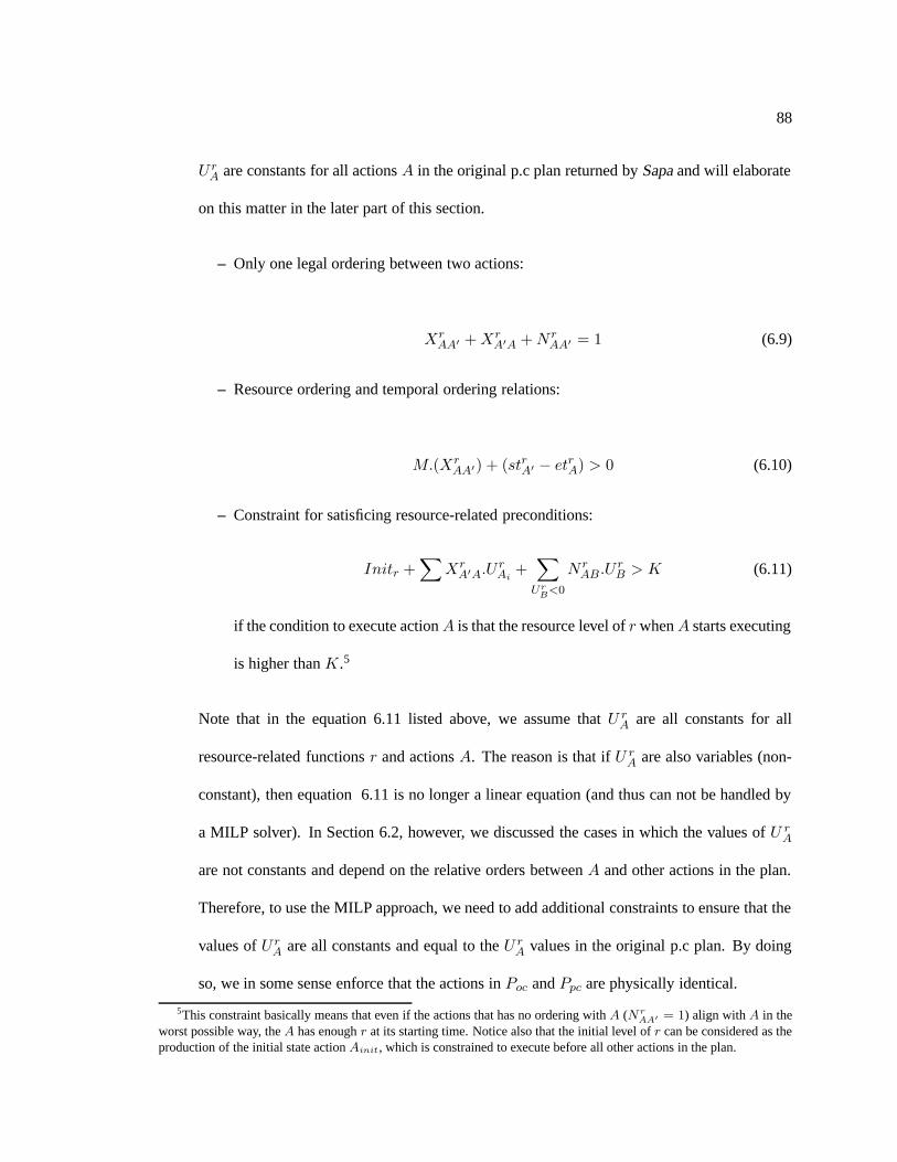
88
U rA are constants for all actions A in the original p.c plan returned by Sapa and will elaborate
on this matter in the later part of this section.
– Only one legal ordering between two actions:
XrAA′ + Xr
A′A + N rAA′ = 1 (6.9)
– Resource ordering and temporal ordering relations:
M.(XrAA′) + (strA′ − etrA) > 0 (6.10)
– Constraint for satisficing resource-related preconditions:
Initr +∑
XrA′A.U r
Ai+
∑
UrB
<0
N rAB .U r
B > K (6.11)
if the condition to execute action A is that the resource level of r when A starts executing
is higher than K .5
Note that in the equation 6.11 listed above, we assume that U rA are all constants for all
resource-related functions r and actions A. The reason is that if U rA are also variables (non-
constant), then equation 6.11 is no longer a linear equation (and thus can not be handled by
a MILP solver). In Section 6.2, however, we discussed the cases in which the values of U rA
are not constants and depend on the relative orders between A and other actions in the plan.
Therefore, to use the MILP approach, we need to add additional constraints to ensure that the
values of U rA are all constants and equal to the U r
A values in the original p.c plan. By doing
so, we in some sense enforce that the actions in Poc and Ppc are physically identical.
5This constraint basically means that even if the actions that has no ordering with A (N rAA′ = 1) align with A in the
worst possible way, the A has enough r at its starting time. Notice also that the initial level of r can be considered as theproduction of the initial state action Ainit, which is constrained to execute before all other actions in the plan.
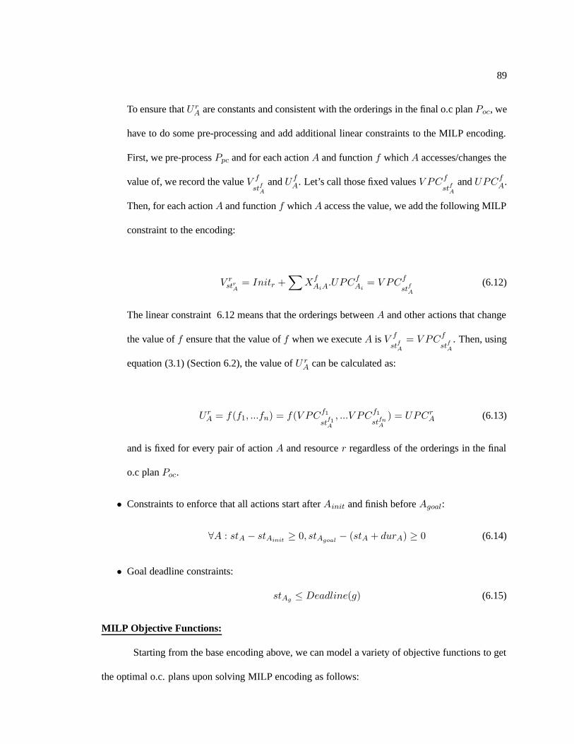
89
To ensure that U rA are constants and consistent with the orderings in the final o.c plan Poc, we
have to do some pre-processing and add additional linear constraints to the MILP encoding.
First, we pre-process Ppc and for each action A and function f which A accesses/changes the
value of, we record the value V f
stfA
and U fA. Let’s call those fixed values V PCf
stfA
and UPCfA.
Then, for each action A and function f which A access the value, we add the following MILP
constraint to the encoding:
V rstr
A= Initr +
∑
XfAiA
.UPCfAi
= V PCf
stfA
(6.12)
The linear constraint 6.12 means that the orderings between A and other actions that change
the value of f ensure that the value of f when we execute A is V f
stfA
= V PCf
stfA
. Then, using
equation (3.1) (Section 6.2), the value of U rA can be calculated as:
U rA = f(f1, ...fn) = f(V PCf1
stf1A
, ...V PCf1
stfnA
) = UPCrA (6.13)
and is fixed for every pair of action A and resource r regardless of the orderings in the final
o.c plan Poc.
• Constraints to enforce that all actions start after Ainit and finish before Agoal:
∀A : stA − stAinit≥ 0, stAgoal
− (stA + durA) ≥ 0 (6.14)
• Goal deadline constraints:
stAg ≤ Deadline(g) (6.15)
MILP Objective Functions:
Starting from the base encoding above, we can model a variety of objective functions to get
the optimal o.c. plans upon solving MILP encoding as follows:
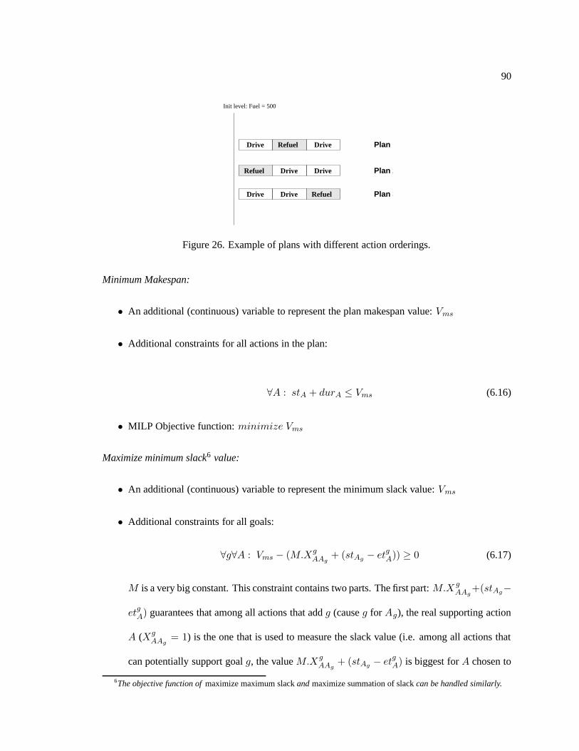
90
Init level: Fuel = 500
Drive
Drive
Drive Drive
Drive Refuel
DriveRefuel
Refuel
Plan 1
Plan 2
Plan 3
Figure 26. Example of plans with different action orderings.
Minimum Makespan:
• An additional (continuous) variable to represent the plan makespan value: Vms
• Additional constraints for all actions in the plan:
∀A : stA + durA ≤ Vms (6.16)
• MILP Objective function: minimize Vms
Maximize minimum slack6 value:
• An additional (continuous) variable to represent the minimum slack value: Vms
• Additional constraints for all goals:
∀g∀A : Vms − (M.XgAAg
+ (stAg − etgA)) ≥ 0 (6.17)
M is a very big constant. This constraint contains two parts. The first part: M.X gAAg
+(stAg−
etgA) guarantees that among all actions that add g (cause g for Ag), the real supporting action
A (XgAAg
= 1) is the one that is used to measure the slack value (i.e. among all actions that
can potentially support goal g, the value M.X gAAg
+ (stAg − etgA) is biggest for A chosen to
6The objective function of maximize maximum slack and maximize summation of slack can be handled similarly.

91
support g). The whole equation with Vms involved would then guarantee that the slack value
is measured correctly. The same big M value is used across all the constraints for different
goals and would be subtracted from the final Vms value to get the correct minimum slack
value.
• MILP objective function: minimize Vms
Minimum number of orderings:
• Additional binary ordering variables for every pair of actions: OAB
• Additional constraints:
∀A,B, p : OAB −XpBA ≥ 0, OAB − Y p
AB ≥ 0 (6.18)
• MILP objective function: minimize ΣOAB
6.5. Partialization: Implementation
We have implemented the greedy variable and value ordering discussed in Section 6.3 and
have also implemented the MILP encoding discussed in Section 6.4. We tested our implementation
as the post-processor in the Sapa planner. While Sapa is quite efficient, it often generates plans
with inferior makespan values. Our aim is to see how much of an improvement the partialization
algorithm provides for the plans produced by Sapa.
Given a p.c plan Ppc, the greedy partialization (GP) and optimal partialization (OP) routines
return three different plans. The first is what we call a logical order constrained (logical o.c) plan. It
consists of a set of logical relations between actions (e.g. causal link from the end point of A1 to the
start point of A2). The logical relations include (i) causal link, (ii) logical mutex, and (iii) resource
mutex. The second is a temporal order constrained (temporal o.c) plan in which the temporal o.c
92
plan is represented by the temporal relations between the starting time points of actions. In short,
we collapse multiple logical relations (in a logical o.c plan) between a pair of actions (A1, A2) into
a single temporal relation between A1 and A2. The temporal o.c plan is actually a Simple Temporal
Network (STN) [18]. While the logical o.c plan gives more information, the temporal o.c plan is
simpler and more compact. Moreover, from the flexibility execution point of view, temporal o.c
plan may be just enough7 . The third plan is the p.c plan sorted from a logical or temporal o.c plan
in which each action is given an earliest starting time allowed by the logical/temporal ordering in
Poc. The makespan of the resulted o.c plan Poc that we report in this section is the makespan of this
p.c plan.
We report the results for the greedy partialization approach in Section 6.5.1 and Sec-
tion 6.5.2. The current empirical results for the optimal partialization using MILP approach are
discussed in Section 6.5.3. The MILP solver that we used is the Java version of the lp solve package,
which can be downloaded from http://www.cs.wustl.edu/j̃avagrp/help/LinearProgramming.html.
The reason that we choose this solve is that it’s also implemented in Java and can thus be inte-
grated into the Sapa package8 .
6.5.1. Greedy Partialization Approach. The first test suite is the 80 random temporal
logistics provided with the TP4 planner. In this planning domain, trucks move packages between
locations inside a city and airplanes move them between cities. Figure 27 shows the comparison
results for only the 20 largest problems, in terms of number of cities and packages, among 80 of
that suite. In the left graph of Figure 27, trucks are allowed to move packages between different
locations in different cities, while in the right graph of the same figure, trucks are not allowed to do
7The temporal o.c plan can be built from a logical o.c plan by sorting the logical relations between each pair of actions.It’s not clear how to build a logical o.c plan from a temporal o.c plan, though.
8In the stand-alone partialization software separated from Sapa, we also allow option to use the external lp solve codeimplemented in C.
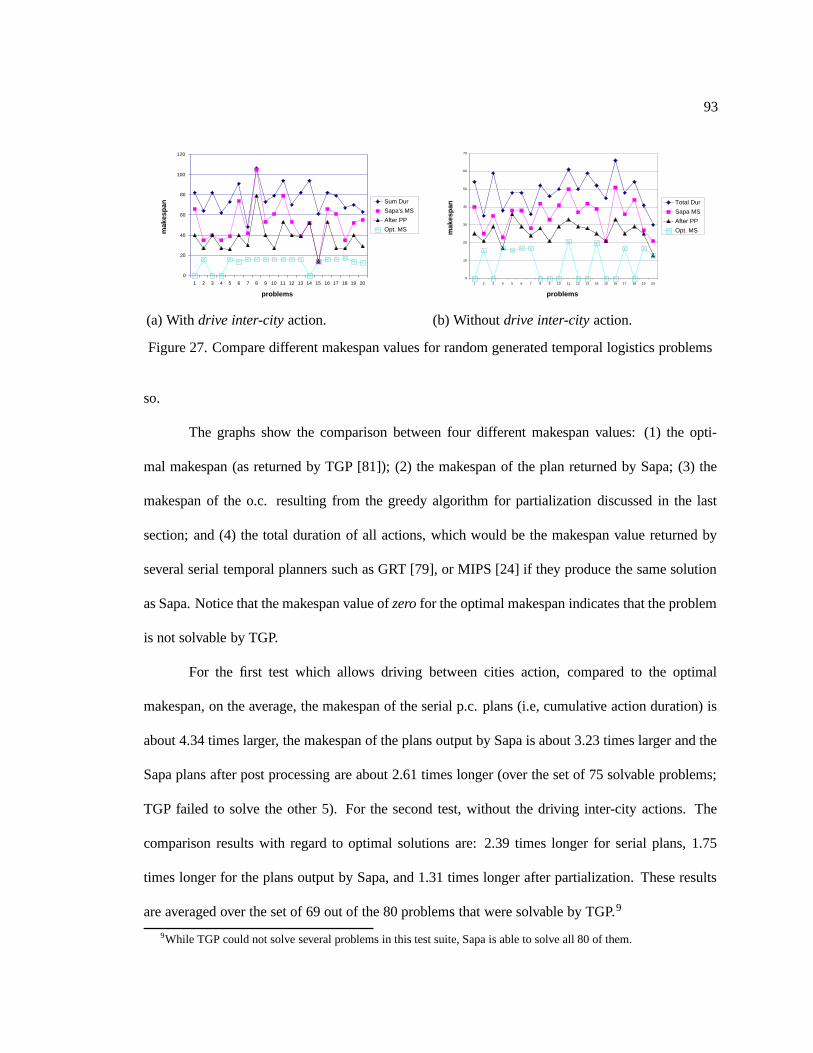
93
0
20
40
60
80
100
120
1 2 3 4 5 6 7 8 9 10 11 12 13 14 15 16 17 18 19 20
problems
mak
esp
an
Sum Dur
Sapa's MS
After PP
Opt. MS
(a) With drive inter-city action.
0
10
20
30
40
50
60
70
1 2 3 4 5 6 7 8 9 10 11 12 13 14 15 16 17 18 19 20
problems
mak
esp
an
Total Dur
Sapa MS
After PP
Opt. MS
(b) Without drive inter-city action.
Figure 27. Compare different makespan values for random generated temporal logistics problems
so.
The graphs show the comparison between four different makespan values: (1) the opti-
mal makespan (as returned by TGP [81]); (2) the makespan of the plan returned by Sapa; (3) the
makespan of the o.c. resulting from the greedy algorithm for partialization discussed in the last
section; and (4) the total duration of all actions, which would be the makespan value returned by
several serial temporal planners such as GRT [79], or MIPS [24] if they produce the same solution
as Sapa. Notice that the makespan value of zero for the optimal makespan indicates that the problem
is not solvable by TGP.
For the first test which allows driving between cities action, compared to the optimal
makespan, on the average, the makespan of the serial p.c. plans (i.e, cumulative action duration) is
about 4.34 times larger, the makespan of the plans output by Sapa is about 3.23 times larger and the
Sapa plans after post processing are about 2.61 times longer (over the set of 75 solvable problems;
TGP failed to solve the other 5). For the second test, without the driving inter-city actions. The
comparison results with regard to optimal solutions are: 2.39 times longer for serial plans, 1.75
times longer for the plans output by Sapa, and 1.31 times longer after partialization. These results
are averaged over the set of 69 out of the 80 problems that were solvable by TGP.9
9While TGP could not solve several problems in this test suite, Sapa is able to solve all 80 of them.
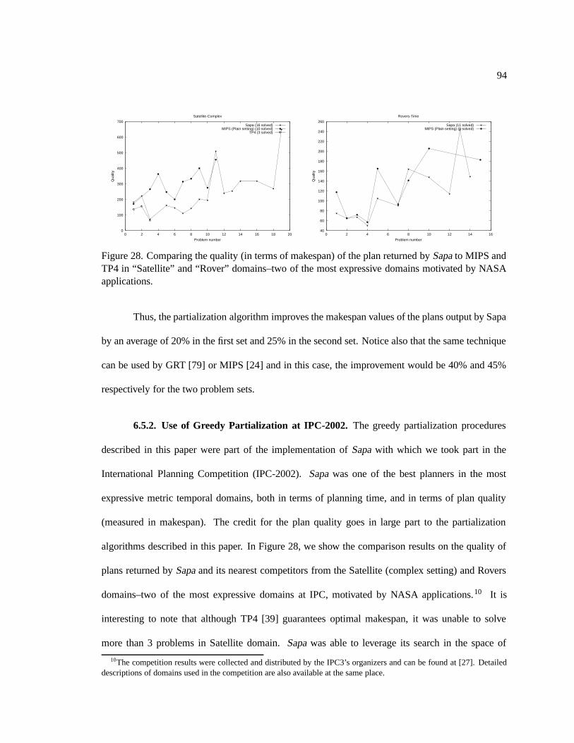
94
0
100
200
300
400
500
600
700
0 2 4 6 8 10 12 14 16 18 20
Qua
lity
Problem number
Satellite-Complex
Sapa (16 solved)MIPS (Plain setting) (10 solved)
TP4 (3 solved)
40
60
80
100
120
140
160
180
200
220
240
260
0 2 4 6 8 10 12 14 16
Qua
lity
Problem number
Rovers-Time
Sapa (11 solved)MIPS (Plain setting) (9 solved)
Figure 28. Comparing the quality (in terms of makespan) of the plan returned by Sapa to MIPS andTP4 in “Satellite” and “Rover” domains–two of the most expressive domains motivated by NASAapplications.
Thus, the partialization algorithm improves the makespan values of the plans output by Sapa
by an average of 20% in the first set and 25% in the second set. Notice also that the same technique
can be used by GRT [79] or MIPS [24] and in this case, the improvement would be 40% and 45%
respectively for the two problem sets.
6.5.2. Use of Greedy Partialization at IPC-2002. The greedy partialization procedures
described in this paper were part of the implementation of Sapa with which we took part in the
International Planning Competition (IPC-2002). Sapa was one of the best planners in the most
expressive metric temporal domains, both in terms of planning time, and in terms of plan quality
(measured in makespan). The credit for the plan quality goes in large part to the partialization
algorithms described in this paper. In Figure 28, we show the comparison results on the quality of
plans returned by Sapa and its nearest competitors from the Satellite (complex setting) and Rovers
domains–two of the most expressive domains at IPC, motivated by NASA applications.10 It is
interesting to note that although TP4 [39] guarantees optimal makespan, it was unable to solve
more than 3 problems in Satellite domain. Sapa was able to leverage its search in the space of
10The competition results were collected and distributed by the IPC3’s organizers and can be found at [27]. Detaileddescriptions of domains used in the competition are also available at the same place.
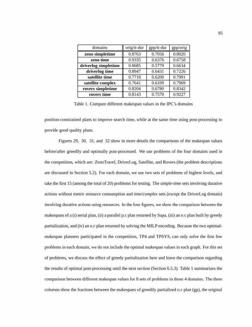
95
domains orig/tt-dur gpp/tt-dur gpp/orig
zeno simpletime 0.8763 0.7056 0.8020zeno time 0.9335 0.6376 0.6758
driverlog simpletime 0.8685 0.5779 0.6634driverlog time 0.8947 0.6431 0.7226satellite time 0.7718 0.6200 0.7991
satellite complex 0.7641 0.6109 0.7969rovers simpletime 0.8204 0.6780 0.8342
rovers time 0.8143 0.7570 0.9227
Table 1. Compare different makespan values in the IPC’s domains
position-constrained plans to improve search time, while at the same time using post-processing to
provide good quality plans.
Figures 29, 30, 31, and 32 show in more details the comparisons of the makespan values
before/after greedily and optimally post-processed. We use problems of the four domains used in
the competition, which are: ZenoTravel, DriverLog, Satellite, and Rovers (the problem descriptions
are discussed in Section 5.2). For each domain, we use two sets of problems of highest levels, and
take the first 15 (among the total of 20) problems for testing. The simple-time sets involving durative
actions without metric resource consumption and time/complex sets (except the DriverLog domain)
involving durative actions using resources. In the four figures, we show the comparison between the
makespans of a (i) serial plan, (ii) a parallel p.c plan returned by Sapa, (iii) an o.c plan built by greedy
partialization, and (iv) an o.c plan returned by solving the MILP encoding. Because the two optimal-
makespan planners participated in the competition, TP4 and TPSYS, can only solve the first few
problems in each domain, we do not include the optimal makespan values in each graph. For this set
of problems, we discuss the effect of greedy partialization here and leave the comparison regarding
the results of optimal post-processing until the next section (Section 6.5.3). Table 1 summarizes the
comparison between different makespan values for 8 sets of problems in those 4 domains. The three
columns show the fractions between the makespans of greedily partialized o.c plan (gp), the original
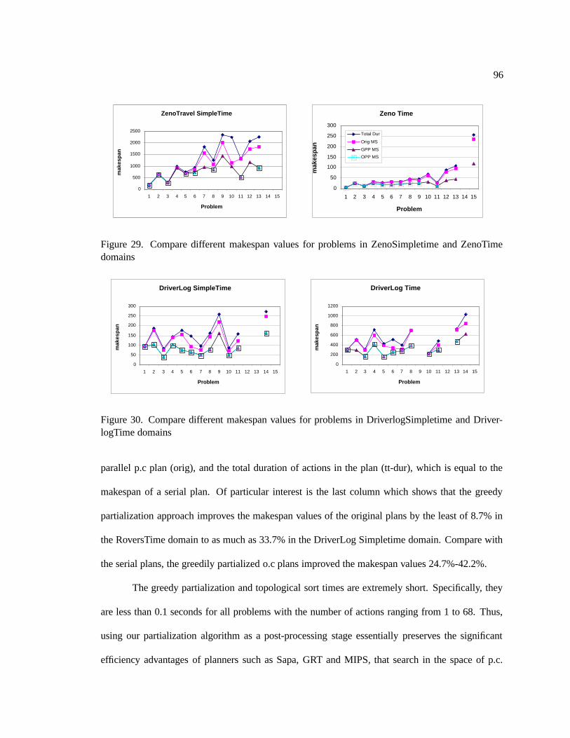
96
ZenoTravel SimpleTime
0
500
1000
1500
2000
2500
1 2 3 4 5 6 7 8 9 10 11 12 13 14 15
Problem
mak
esp
an
Zeno Time
0
50
100
150
200
250
300
1 2 3 4 5 6 7 8 9 10 11 12 13 14 15
Problem
mak
esp
an
Total Dur
Orig MS
GPP MS
OPP MS
Figure 29. Compare different makespan values for problems in ZenoSimpletime and ZenoTimedomains
DriverLog SimpleTime
0
50
100
150
200
250
300
1 2 3 4 5 6 7 8 9 10 11 12 13 14 15
Problem
mak
esp
an
DriverLog Time
0
200
400
600
800
1000
1200
1 2 3 4 5 6 7 8 9 10 11 12 13 14 15
Problem
mak
esp
an
Figure 30. Compare different makespan values for problems in DriverlogSimpletime and Driver-logTime domains
parallel p.c plan (orig), and the total duration of actions in the plan (tt-dur), which is equal to the
makespan of a serial plan. Of particular interest is the last column which shows that the greedy
partialization approach improves the makespan values of the original plans by the least of 8.7% in
the RoversTime domain to as much as 33.7% in the DriverLog Simpletime domain. Compare with
the serial plans, the greedily partialized o.c plans improved the makespan values 24.7%-42.2%.
The greedy partialization and topological sort times are extremely short. Specifically, they
are less than 0.1 seconds for all problems with the number of actions ranging from 1 to 68. Thus,
using our partialization algorithm as a post-processing stage essentially preserves the significant
efficiency advantages of planners such as Sapa, GRT and MIPS, that search in the space of p.c.
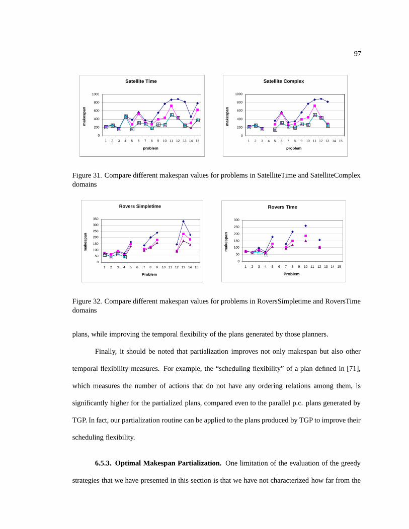
97
Satellite Time
0
200
400
600
800
1000
1 2 3 4 5 6 7 8 9 10 11 12 13 14 15
problem
mak
esp
an
Satellite Complex
0
200
400
600
800
1000
1 2 3 4 5 6 7 8 9 10 11 12 13 14 15
problem
mak
esp
an
Figure 31. Compare different makespan values for problems in SatelliteTime and SatelliteComplexdomains
Rovers Simpletime
0
50
100
150
200
250
300
350
1 2 3 4 5 6 7 8 9 10 11 12 13 14 15
Problem
mak
esp
an
Rovers Time
0
50
100
150
200
250
300
1 2 3 4 5 6 7 8 9 10 11 12 13 14 15
Problem
mak
esp
an
Figure 32. Compare different makespan values for problems in RoversSimpletime and RoversTimedomains
plans, while improving the temporal flexibility of the plans generated by those planners.
Finally, it should be noted that partialization improves not only makespan but also other
temporal flexibility measures. For example, the “scheduling flexibility” of a plan defined in [71],
which measures the number of actions that do not have any ordering relations among them, is
significantly higher for the partialized plans, compared even to the parallel p.c. plans generated by
TGP. In fact, our partialization routine can be applied to the plans produced by TGP to improve their
scheduling flexibility.
6.5.3. Optimal Makespan Partialization. One limitation of the evaluation of the greedy
strategies that we have presented in this section is that we have not characterized how far from the
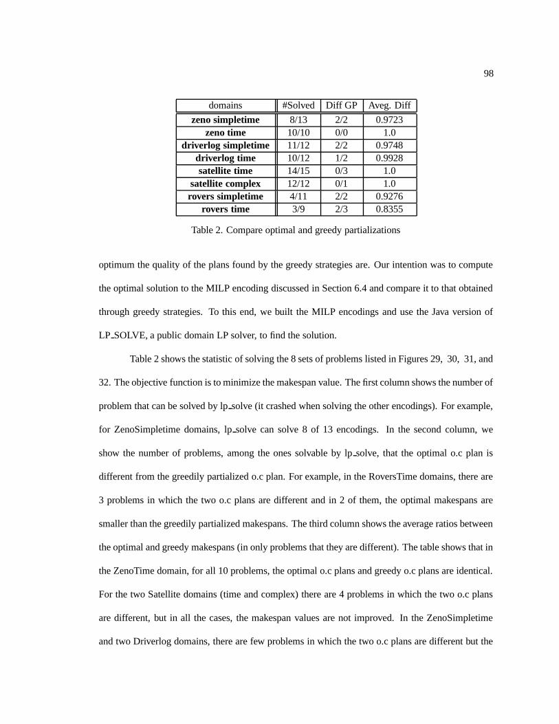
98
domains #Solved Diff GP Aveg. Diff
zeno simpletime 8/13 2/2 0.9723zeno time 10/10 0/0 1.0
driverlog simpletime 11/12 2/2 0.9748driverlog time 10/12 1/2 0.9928satellite time 14/15 0/3 1.0
satellite complex 12/12 0/1 1.0rovers simpletime 4/11 2/2 0.9276
rovers time 3/9 2/3 0.8355
Table 2. Compare optimal and greedy partializations
optimum the quality of the plans found by the greedy strategies are. Our intention was to compute
the optimal solution to the MILP encoding discussed in Section 6.4 and compare it to that obtained
through greedy strategies. To this end, we built the MILP encodings and use the Java version of
LP SOLVE, a public domain LP solver, to find the solution.
Table 2 shows the statistic of solving the 8 sets of problems listed in Figures 29, 30, 31, and
32. The objective function is to minimize the makespan value. The first column shows the number of
problem that can be solved by lp solve (it crashed when solving the other encodings). For example,
for ZenoSimpletime domains, lp solve can solve 8 of 13 encodings. In the second column, we
show the number of problems, among the ones solvable by lp solve, that the optimal o.c plan is
different from the greedily partialized o.c plan. For example, in the RoversTime domains, there are
3 problems in which the two o.c plans are different and in 2 of them, the optimal makespans are
smaller than the greedily partialized makespans. The third column shows the average ratios between
the optimal and greedy makespans (in only problems that they are different). The table shows that in
the ZenoTime domain, for all 10 problems, the optimal o.c plans and greedy o.c plans are identical.
For the two Satellite domains (time and complex) there are 4 problems in which the two o.c plans
are different, but in all the cases, the makespan values are not improved. In the ZenoSimpletime
and two Driverlog domains, there are few problems in which the two o.c plans are different but the
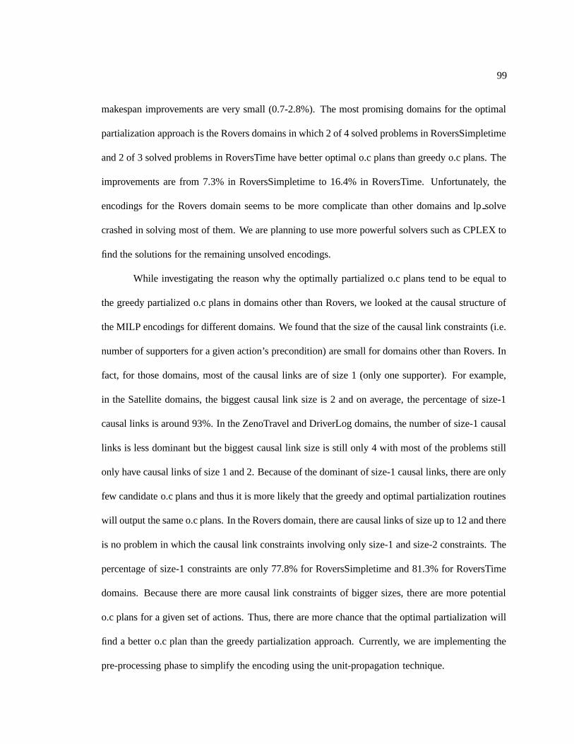
99
makespan improvements are very small (0.7-2.8%). The most promising domains for the optimal
partialization approach is the Rovers domains in which 2 of 4 solved problems in RoversSimpletime
and 2 of 3 solved problems in RoversTime have better optimal o.c plans than greedy o.c plans. The
improvements are from 7.3% in RoversSimpletime to 16.4% in RoversTime. Unfortunately, the
encodings for the Rovers domain seems to be more complicate than other domains and lp solve
crashed in solving most of them. We are planning to use more powerful solvers such as CPLEX to
find the solutions for the remaining unsolved encodings.
While investigating the reason why the optimally partialized o.c plans tend to be equal to
the greedy partialized o.c plans in domains other than Rovers, we looked at the causal structure of
the MILP encodings for different domains. We found that the size of the causal link constraints (i.e.
number of supporters for a given action’s precondition) are small for domains other than Rovers. In
fact, for those domains, most of the causal links are of size 1 (only one supporter). For example,
in the Satellite domains, the biggest causal link size is 2 and on average, the percentage of size-1
causal links is around 93%. In the ZenoTravel and DriverLog domains, the number of size-1 causal
links is less dominant but the biggest causal link size is still only 4 with most of the problems still
only have causal links of size 1 and 2. Because of the dominant of size-1 causal links, there are only
few candidate o.c plans and thus it is more likely that the greedy and optimal partialization routines
will output the same o.c plans. In the Rovers domain, there are causal links of size up to 12 and there
is no problem in which the causal link constraints involving only size-1 and size-2 constraints. The
percentage of size-1 constraints are only 77.8% for RoversSimpletime and 81.3% for RoversTime
domains. Because there are more causal link constraints of bigger sizes, there are more potential
o.c plans for a given set of actions. Thus, there are more chance that the optimal partialization will
find a better o.c plan than the greedy partialization approach. Currently, we are implementing the
pre-processing phase to simplify the encoding using the unit-propagation technique.
100
6.6. Summary and Discussion
In this chapter, we present an approach of encoding the partialization problem as Constraint
Satisfaction Optimization Problem (CSOP). We also implemented two different ways of solving this
CSOP encoding, either greedily in linear time or optimally by converting it into a MILP encoding.
Those techniques can be used in Sapa and other state-space search planners to generate more flexible
order-constrained plans, or to improve the makespan values of the final plan.
To extend the work on partialization in this chapter, we are currently focusing on:
• Improving the optimal solving of the CSOP encodings (Section 6.4): the first idea in mind is
to use a more powerful MILP solver (e.g. CPLEX). Given that a large portion of the encoding
involving binary variables, other types of solvers besides the pure MILP solver can potentially
be the better fits. The first approach is to follow the LPSAT [97] approach and separate the
use the SAT solver (which is specifically designed for boolean variables) to handle the binary
MILP variables and constraints involving them. The continuous value variables representing
action starting times are then managed using a LP encoding. Besides this coupled framework,
using CSOP solver to directly solve our CSOP encoding, which involves both discrete and
continuous variables is also promising. Previously, we could not find a suitable CSOP solver
for this task. However, the CSOP solver used in the recently-developed CPT [91] planner
appears to be a good candidate. Given that the CPT’s encoding seems to be much bigger than
our encoding (in terms of involving variables) and its good performance. To use this solver,
we may need to make some adjustments: (i) while metric resource related constraints also
involve continuous variables like temporal constraints, they are different and thus the base
solver may need extensions to handle them; (ii) the variable and value orderings are aimed
toward the objective function of minimizing plan’s makespan value. Therefore, different
101
heuristics are needed for other objective functions discussed in Section 6.2.
• Based on the observation that there is a large portion of the supporting constraints (i.e. spec-
ifying the supporter for a given action precondition) involving only a single supporter, we
can significantly reduce the number of variables and constraints by pre-assigning values to
those variables and simplifying the other constraints. Therefore, we are implementing a pre-
processing routine based on unit propagation and hope that it can speedup the solver by sig-
nificantly simplifying the encoding.
CHAPTER 7
Adapting Best-First Search to Partial-Satisfaction Planning
Many metric temporal planning problems can be characterized as over-subscription prob-
lems (c.f. Smith([84, 85])) in that goals have different values and the planning system must choose
a subset that can be achieved within the time and resource limits. This type of problem is more
general than the ones we have been concentrated on so far in this dissertation where all the goals
need to be achieved for the plan to be valid. Examples of the over-subscription problems include
many of NASA planning problems such as planning for telescopes like Hubble[56], SIRTF[57],
Landsat 7 Satellite[78]; and planning science for Mars rover [84]. Given the resource and time
limits, only certain set of goals can be achieved and thus it is best to achieve the subset of goals that
have highest total value given those constraints. In this dissertation, we consider a subclass of the
over-subscription problem where goals have different utility (or values) and actions incur different
execution costs, which are generally defined by the amount of resource (e.g. money, fuel) consump-
tion and the temporal aspect of that action (e.g how much time spent executing that action). The
objective is then to find the most beneficial plan, that is the plan with the best tradeoff between
the total benefit of achieved goals and the total execution cost of actions in the plan. We refer to
this subclass of the over-subscription problem as Partial-Satisfaction Planning (PSP) Net Benefit
problem where not all the goals need to be satisfied by the final plan. In this chapter, we present the
extensions to the Sapa’s search algorithm to solve PSP Net Benefit problems. Later, we also discuss
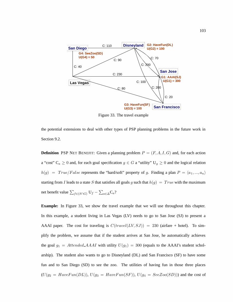
103
Disneyland
San Jose
San Francisco
Las Vegas
G1: AAAI(SJ)U(G1) = 300
G3: HaveFun(SF)U(G3) = 100
G2: HaveFun(DL)U(G2) = 100
C: 20
C: 70
C: 230
C: 80
C: 90
C: 200
C: 200
C: 100
San DiegoG4: SeeZoo(SD)U(G4) = 50
C: 40
C: 110
Figure 33. The travel example
the potential extensions to deal with other types of PSP planning problems in the future work in
Section 9.2.
Definition PSP NET BENEFIT: Given a planning problem P = (F,A, I,G) and, for each action
a “cost” Ca ≥ 0 and, for each goal specification g ∈ G a “utility” Ug ≥ 0 and the logical relation
h(g) = True/False represents the “hard/soft” property of g. Finding a plan P = 〈a1, ..., an〉
starting from I leads to a state S that satisfies all goals g such that h(g) = True with the maximum
net benefit value∑
f∈(S∩G) Uf −∑
a∈∆Ca?
Example: In Figure 33, we show the travel example that we will use throughout this chapter.
In this example, a student living in Las Vegas (LV) needs to go to San Jose (SJ) to present a
AAAI paper. The cost for traveling is C(travel(LV, SJ)) = 230 (airfare + hotel). To sim-
plify the problem, we assume that if the student arrives at San Jose, he automatically achieves
the goal g1 = Attended AAAI with utility U(g1) = 300 (equals to the AAAI’s student schol-
arship). The student also wants to go to Disneyland (DL) and San Francisco (SF) to have some
fun and to San Diego (SD) to see the zoo. The utilities of having fun in those three places
(U(g2 = HaveFun(DL)), U(g3 = HaveFun(SF )), U(g4 = SeeZoo(SD))) and the cost of
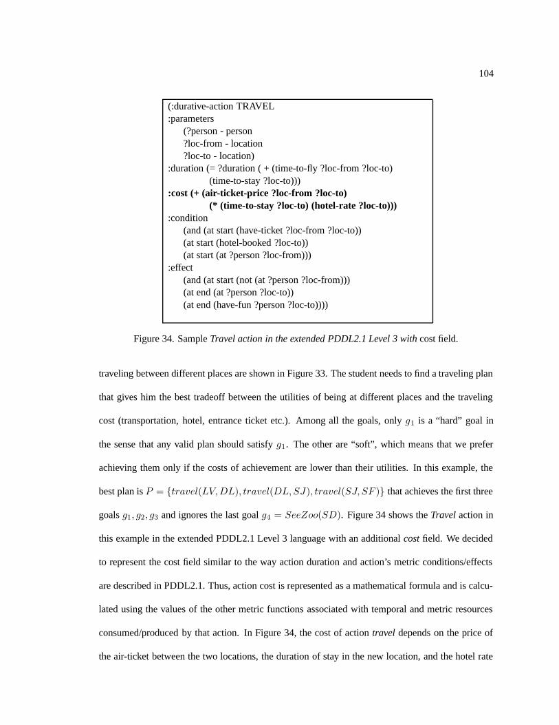
104
(:durative-action TRAVEL:parameters
(?person - person?loc-from - location?loc-to - location)
:duration (= ?duration ( + (time-to-fly ?loc-from ?loc-to)(time-to-stay ?loc-to)))
:cost (+ (air-ticket-price ?loc-from ?loc-to)(* (time-to-stay ?loc-to) (hotel-rate ?loc-to)))
:condition(and (at start (have-ticket ?loc-from ?loc-to))(at start (hotel-booked ?loc-to))(at start (at ?person ?loc-from)))
:effect(and (at start (not (at ?person ?loc-from)))(at end (at ?person ?loc-to))(at end (have-fun ?person ?loc-to))))
Figure 34. Sample Travel action in the extended PDDL2.1 Level 3 with cost field.
traveling between different places are shown in Figure 33. The student needs to find a traveling plan
that gives him the best tradeoff between the utilities of being at different places and the traveling
cost (transportation, hotel, entrance ticket etc.). Among all the goals, only g1 is a “hard” goal in
the sense that any valid plan should satisfy g1. The other are “soft”, which means that we prefer
achieving them only if the costs of achievement are lower than their utilities. In this example, the
best plan is P = {travel(LV,DL), travel(DL,SJ), travel(SJ, SF )} that achieves the first three
goals g1, g2, g3 and ignores the last goal g4 = SeeZoo(SD). Figure 34 shows the Travel action in
this example in the extended PDDL2.1 Level 3 language with an additional cost field. We decided
to represent the cost field similar to the way action duration and action’s metric conditions/effects
are described in PDDL2.1. Thus, action cost is represented as a mathematical formula and is calcu-
lated using the values of the other metric functions associated with temporal and metric resources
consumed/produced by that action. In Figure 34, the cost of action travel depends on the price of
the air-ticket between the two locations, the duration of stay in the new location, and the hotel rate
105
at that locations. In Section 7.3, we discuss in more details how to generate the PSP problems for
benchmark domains and the full description of several domains are presented in the Appendix A.3.
Sapa and most of the current planning systems are not designed to solve the over-
subscription or PSP problems. Most of them expect a set of conjunctive goals of equal value and
the planning process does not terminate until all the goals are achieved. Extending the traditional
planning techniques to solve the PSP Net Benefit problem poses several challenges:
• The termination criteria for the planning process change because there are no fixed set of
conjunctive goals to satisfy.
• Heuristic guidance in the traditional planning systems are designed to guide the planners to
achieve a fixed set of goals. They can not be used directly in the over-subscription problem.
• Plan quality should take into account not only action costs but also the values of goals
achieved by the final plan.
Over-subscription problems have received some attention in scheduling, using the “greedy”
approaches. Straight forward adaptation to planning would involve considering goals in the de-
creasing order of their values. However, goals with higher values may also be more expensive to
achieve and thus may give the cost vs. benefit tradeoff that is far from optimal. Moreover, inter-
actions between goals may make the cost/benefit to achieve a set of goals quite different from the
value of individual goals. Recently, Smith ([85]) and van den Briel et. al ([89]) discuss two ap-
proaches for solving partial satisfaction planning problems by heuristically selecting a subset S of
goals that appear to be the most beneficial and then use the normal planning search to find the least
cost solution that achieves all goals in S. If there are n goals then this approach would essentially
involve selecting the most beneficial subset of goals among a total of 2n choices. While this type
of approach is less susceptible to inoptimal plans compared to the naive greedy approach, it too is
106
overly dependent on the informedness of the initial goal-set selection heuristic. If the heuristic is
not informed, then there can be beneficial goals left out and S may contain unbeneficial goals.
In this chapter, we investigate heuristic algorithms based on best-first search for solving
PSP NET BENEFIT. Sapaps , an extension of Sapa for solving PSP Net Benefit, uses an anytime
heuristic search framework in which goals are treated as a mixture of “soft” and “hard” constraints.
Thus, among all the goals in G, only a subset GH contains “hard goals” that need to be satisfied
for the plan to be valid. The remaining goals in GS = G \ GH are “soft” and achieving them only
affects the quality of the final plan but not the validity of the plan. The search framework does not
concentrate on achieving a particular subset of goals, but rather decides what is the best solution
for each node in the search tree. Any executable plan that achieves all “hard” goals is considered
a potential solution, with the quality of the plan measured in terms of its net benefit. The objective
of the search is to find the plan with the highest net benefit. Sapaps uses novel ways of estimating
the g and h values of partial solutions, and uses them to guide an anytime A* search. In particular,
the evaluations of the g and h values of nodes in the A* search tree are based on the subset of goals
achieved in the current search node and the best potential beneficial plan from the current state
to achieve a subset of the remaining goals. We show that Sapaps can produce high quality plans
compared to the greedy approach.
For the remaining of this chapter, we will first present the any-time algorithm in Section 7.1.
This algorithm and the heuristic guiding it are extended from the forward search algorithm and plan-
ning graph based heuristics discussed in Chapter 3 and 4. The heuristic used in Sapaps is discussed
in Section 7.2 and the empirical results are presented in Section 7.3. For reference, the examples
for the extended version of PDDL2.1 representing the PSP Net Benefit problem are provided in the
Appendix A.3.
107
7.1. Anytime Search Algorithm for PSP Net Benefit
Most of the current successful heuristic planners [7, 41, 70, 22, 25], including Sapa, use
weighted A* search with heuristic guidances extracted from solving the relaxed problem ignoring
the delete list. In the heuristic formula f = g + w ∗ h guiding the weighted A* search, the g value
is measured by the total cost of actions leading to the current state and the h value is the estimated
total action cost to achieve all goals from the current state (forward planner) or to reach the current
state from the initial state (backward planner). Compared to the traditional planning problem, the
PSP problem has new requirements: (i) goals have different utility values; (ii) not all the goals need
to be accomplished in the final plan; (iii) the plan quality is not measured by the total action cost but
the tradeoff between the total achieved goals’ utilities and the total action cost. Therefore, in order
to employ the A* search, we need to modify the way each search node is evaluated as well as the
criteria used to terminate the search process.1
In this section, we discuss a method which models the top-level goals G as “soft” and “hard”
constraints (G = GS⋃
GH ). All executable plans that achieve all goals in GH are considered
potential solutions, or valid plans. The quality of a valid plan is then measured in terms of its net
benefit and the objective of the search is then to find a valid plan with the highest net benefit. To
model this search problem in an A* framework, we need to first define the g and h values of a partial
plan. The g value will need to capture the current net benefit of the plan, while the h value needs to
estimate the net benefit that can be potentially accrued by extending the plan to cover more goals.
Once we have these definitions, we need methods for efficiently estimating the the h value. We
will detail this process in the context of Sapaps , which is an extension of Sapa and does forward
(progression) search in the space of states.
1To avoid confusion, we will concentrate the discussion on the new A* search framework in the context of a forwardplanner. It can also be used in regression planners by reversing the search direction.
108
g value: In forward planners, applicable actions are executed in the current state to generate new
states. Generated nodes are sorted in the queue by their f values. The search stops when the first
node taken from the queue satisfies all the pre-defined conjunctive goals. In our ongoing example,
at the initial state Sinit = {at(LV )}, there are four applicable actions A1 = travel(LV,DL),
A2 = travel(LV, SJ), A3 = travel(LV, SF ) and A4 = travel(LV, SD) that lead to four states
S1 = {at(DL), g2}, S2 = {at(SJ), g1}, S3 = {at(SF ), g3}, and S4 = {at(SD), g4}. Assume
that we pick state S1 from the queue, then applying action A5 = travel(DL,SF ) to S1 would lead
to state S5 = {at(SF ), g2, g3}.
For a given state S, let partial plan PP (S) be the plan leading from the initial state Sinit to
S, and the goal set G(S) be the set of goals accomplished in S. The overall quality of the state S
depends on the total utility of the goals in G(S) and the costs of actions in PP (S). The g value is
thus defined as :
g(S) = U(G(S)) − C(PP (S)) (7.1)
Where U(G(S)) =∑
g∈G(S) Ug is the total utility of the goals in G(S), and C(PP (S)) =
∑
a∈PP (S) Ca is the total cost of actions in PP (S). In our ongoing example, at the initial
state Sinit = {at(LV )}. Applying action a1 = travel(LV,DL) would leads to the state
S1 = {at(DL), g2} and applying action a2 = travel(DL,SF ) to S1 would lead to state
S2 = {at(SF ), g2, g3}. Thus, for state S2, the total utility and cost values are: U(G(S2)) =
Ug2+ Ug3
= 100 + 100 = 200, and C(PP (S2)) = Ca1+ Ca2
= 90 + 100 = 190.
h value: The h value of a state S should estimate how much additional net benefit can be accrued
by extending the partial plan PS to achieve additional goals beyond G(S). The perfect heuristic
function h∗ would give the maximum net benefit that can be accrued. Any h function that is an
upper bound on h∗ will be admissible (notice that we are considering the maximizing variant of
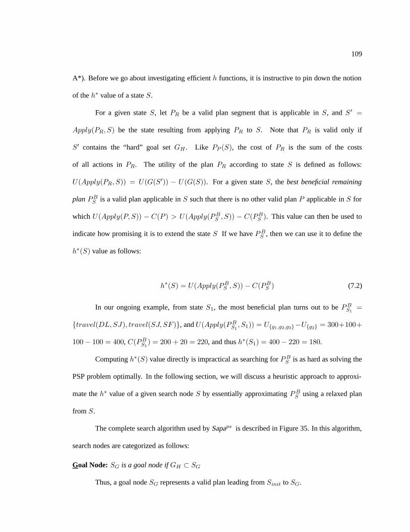
109
A*). Before we go about investigating efficient h functions, it is instructive to pin down the notion
of the h∗ value of a state S.
For a given state S, let PR be a valid plan segment that is applicable in S, and S ′ =
Apply(PR, S) be the state resulting from applying PR to S. Note that PR is valid only if
S′ contains the “hard” goal set GH . Like PP (S), the cost of PR is the sum of the costs
of all actions in PR. The utility of the plan PR according to state S is defined as follows:
U(Apply(PR, S)) = U(G(S ′)) − U(G(S)). For a given state S, the best beneficial remaining
plan P BS is a valid plan applicable in S such that there is no other valid plan P applicable in S for
which U(Apply(P, S)) − C(P ) > U(Apply(P BS , S)) − C(P B
S ). This value can then be used to
indicate how promising it is to extend the state S If we have P BS , then we can use it to define the
h∗(S) value as follows:
h∗(S) = U(Apply(P BS , S)) −C(P B
S ) (7.2)
In our ongoing example, from state S1, the most beneficial plan turns out to be P BS1
=
{travel(DL,SJ), travel(SJ, SF )}, and U(Apply(P BS1
, S1)) = U{g1,g2,g3}−U{g2} = 300+100+
100 − 100 = 400, C(P BS1
) = 200 + 20 = 220, and thus h∗(S1) = 400− 220 = 180.
Computing h∗(S) value directly is impractical as searching for P BS is as hard as solving the
PSP problem optimally. In the following section, we will discuss a heuristic approach to approxi-
mate the h∗ value of a given search node S by essentially approximating P BS using a relaxed plan
from S.
The complete search algorithm used by Sapaps is described in Figure 35. In this algorithm,
search nodes are categorized as follows:
Goal Node: SG is a goal node if GH ⊂ SG
Thus, a goal node SG represents a valid plan leading from Sinit to SG.
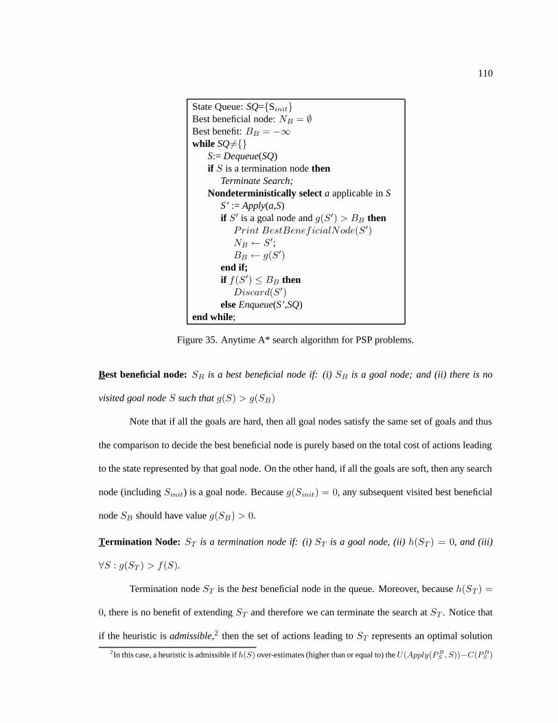
110
State Queue: SQ={Sinit}Best beneficial node: NB = ∅Best benefit: BB = −∞while SQ6={}
S:= Dequeue(SQ)if S is a termination node then
Terminate Search;Nondeterministically select a applicable in S
S’ := Apply(a,S)if S′ is a goal node and g(S ′) > BB then
Print BestBeneficialNode(S ′)NB ← S′;BB ← g(S′)
end if;if f(S′) ≤ BB then
Discard(S ′)else Enqueue(S’,SQ)
end while;
Figure 35. Anytime A* search algorithm for PSP problems.
Best beneficial node: SB is a best beneficial node if: (i) SB is a goal node; and (ii) there is no
visited goal node S such that g(S) > g(SB)
Note that if all the goals are hard, then all goal nodes satisfy the same set of goals and thus
the comparison to decide the best beneficial node is purely based on the total cost of actions leading
to the state represented by that goal node. On the other hand, if all the goals are soft, then any search
node (including Sinit) is a goal node. Because g(Sinit) = 0, any subsequent visited best beneficial
node SB should have value g(SB) > 0.
Termination Node: ST is a termination node if: (i) ST is a goal node, (ii) h(ST ) = 0, and (iii)
∀S : g(ST ) > f(S).
Termination node ST is the best beneficial node in the queue. Moreover, because h(ST ) =
0, there is no benefit of extending ST and therefore we can terminate the search at ST . Notice that
if the heuristic is admissible,2 then the set of actions leading to ST represents an optimal solution
2In this case, a heuristic is admissible if h(S) over-estimates (higher than or equal to) the U(Apply(P BS , S))−C(P B
S )
111
for the PSP problem.
Unpromising Node: S is a unpromising node if f(S) ≤ g(SB) with SB is a best beneficial node
visited so far.
The net benefit value of the best beneficial node (BB) found during search can be used to
set up the lower-bound value and thus nodes that have f values smaller than that lower-bound can
be discarded. Thus, if the heuristic is “perfect”, then unpromising nodes can never be extended to
reach state which is more beneficial than the best plan found so far during search.
As described in Figure 35, the search algorithm starts with the initial state Sinit and keeps
dequeuing the best promising node S (i.e. highest f value). If S is a termination node, then we stop
the search. If not, then we extend S by applying applicable actions a to S. If the newly generated
node S′ = Apply(a, S) is a goal node and has a better g(S ′) value than the best beneficial node
visited so far, then we print the plan leading from Sinit to S′. Finally, if S ′ is not a unpromising node,
then we will put it in the search queue SQ sorted in the decreasing order of f values. Notice that
because we keep outputting the best beneficial nodes while conducting search (until a terminal node
is found), this is an anytime algorithm. The benefit of this approach is that the planner can return
some plan with a positive net-benefit fast and keep on returning plans with better net benefit, if given
more time to do more search. Thus, we can impose the time or search node limit on the algorithm
and try to find the best plan within those limits. To demonstrate the anytime search framework, let’s
assume that the nodes S1, S2, S3, S4 are generated in that order when we extend Sinit. Starting with
the best benefit value of BB = −∞, the planner will first generate the plan P1 = PP (S1) = A1
leading to S1, even though g(S1) = 100 − 90 = 10 > BB = −∞, S1 is not a goal node and thus
P1 is not a valid plan. Then, when S2 is generated, because g(S2) = 70 > BB = −∞ and S2
satisfies the only hard goal g1, the planner outputs P2 = PP (S2) = A2 as the first best plan. Nodes
value.
112
0
Cost
Time52.5 3.5
300
180
90
Travel(SJ,DL)
Travel(SF,DL)
Travel(LV,DL)
Figure 36. Cost function of goal At(DL)
S3 and S4 are less beneficial and are just put back in SQ. Assuming perfect heuristic,3 the planner
will pick S1 to extend. By applying action A7 = travel(DL,SJ) to S1, we get to state S7 that is
more beneficial than the best state visited (g(S7) = 400 − 290 = 110 > BB = 70) and is also a
goal node. Therefore, we will output P3 = PP (S7) = {travel(LV,DL), travel(DL,SJ)}. The
algorithm continues until we reach the termination node S8 = Apply(travel(SJ, SF ), S7).
Notice that while the categorization of nodes was based on “perfect” heuristic, the current
heuristic used in Sapaps is not admissible. Therefore: (i) a pruned unpromising nodes may actually
be promising (i.e. extendible to reach node S with g(S) > BB); and (ii) a termination node may
not be the best beneficial node. In our implementation, even though weight w = 1 is used in
equation f = g + w ∗ h to sort nodes in the queue, another value w = 2 is used for pruning
(unpromising) nodes with f = g + w ∗ h ≤ BB . Thus, only nodes S with estimated heuristic value
h(S) ≤ 1/w ∗ h∗(S) are pruned. For the second issue, we can continue the search for a better
beneficial nodes after a termination node is found until some criteria are met (e.g. reached certain
number of search node limit).
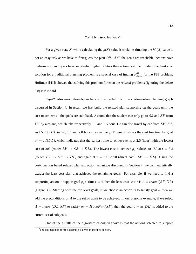
113
7.2. Heuristic for Sapaps
For a given state S, while calculating the g(S) value is trivial, estimating the h∗(S) value is
not an easy task as we have to first guess the plan P BS . If all the goals are reachable, actions have
uniform cost and goals have substantial higher utilities than action cost then finding the least cost
solution for a traditional planning problem is a special case of finding P BSinit
for the PSP problem.
Hoffman ([41]) showed that solving this problem for even the relaxed problems (ignoring the delete
list) is NP-hard.
Sapaps also uses relaxed-plan heuristic extracted from the cost-sensitive planning graph
discussed in Section 4. In recall, we first build the relaxed plan supporting all the goals until the
cost to achieve all the goals are stabilized. Assume that the student can only go to SJ and SF from
LV by airplane, which take respectively 1.0 and 1.5 hour. He can also travel by car from LV , SJ ,
and SF to DL in 5.0, 1.5 and 2.0 hours, respectively. Figure 36 shows the cost function for goal
g2 = At(DL), which indicates that the earliest time to achieve g2 is at 2.5 (hour) with the lowest
cost of 300 (route: LV → SJ → DL). The lowest cost to achieve g2 reduces to 180 at t = 3.5
(route: LV → SF → DL) and again at t = 5.0 to 90 (direct path: LV → DL). Using the
cost-function based relaxed plan extraction technique discussed in Section 4, we can heuristically
extract the least cost plan that achieves the remaining goals. For example, if we need to find a
supporting action to support goal g2 at time t = 4, then the least cost action is A = travel(SF,DL)
(Figure 36). Starting with the top level goals, if we choose an action A to satisfy goal g, then we
add the preconditions of A to the set of goals to be achieved. In our ongoing example, if we select
A = travel(DL,SF ) to satisfy g3 = HaveFun(SF ), then the goal g = at(DL) is added to the
current set of subgoals.
One of the pitfalls of the algorithm discussed above is that the actions selected to support
3The optimal plan for this example is given in the first section.
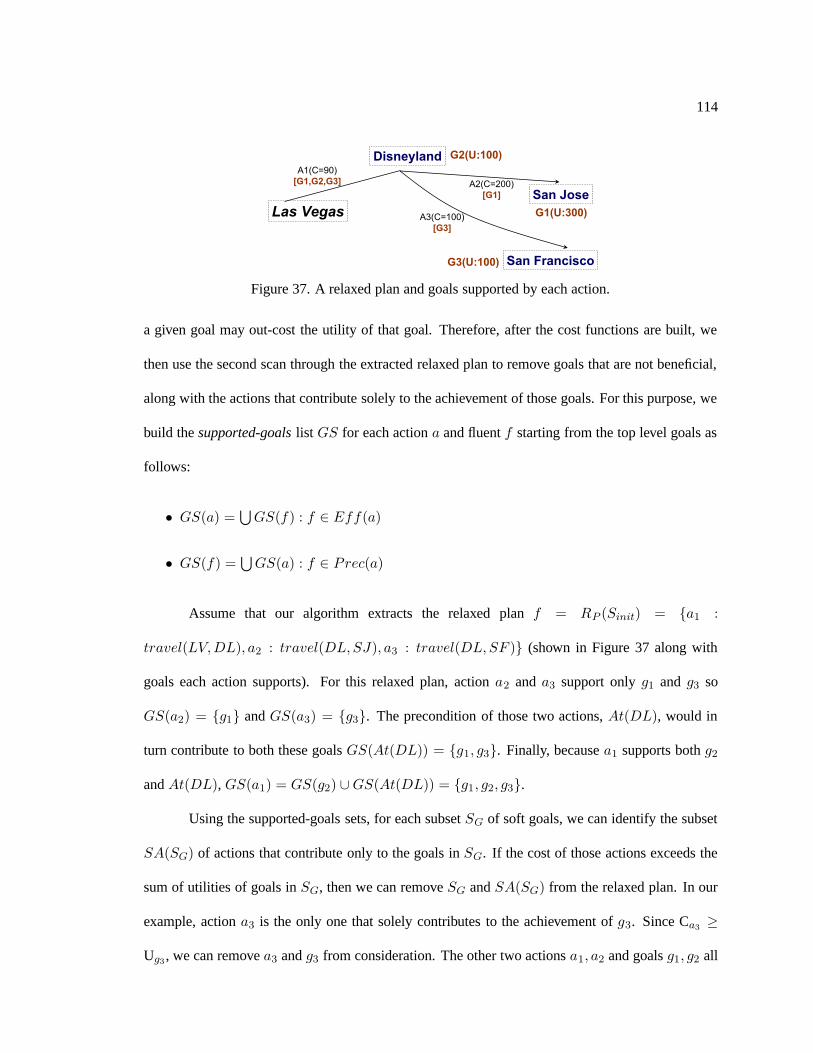
114
Disneyland
San Jose
San Francisco
Las Vegas G1(U:300)
G3(U:100)
G2(U:100)
A1(C=90)
[G1,G2,G3] A2(C=200)
[G1]
A3(C=100)
[G3]
Figure 37. A relaxed plan and goals supported by each action.
a given goal may out-cost the utility of that goal. Therefore, after the cost functions are built, we
then use the second scan through the extracted relaxed plan to remove goals that are not beneficial,
along with the actions that contribute solely to the achievement of those goals. For this purpose, we
build the supported-goals list GS for each action a and fluent f starting from the top level goals as
follows:
• GS(a) =⋃
GS(f) : f ∈ Eff(a)
• GS(f) =⋃
GS(a) : f ∈ Prec(a)
Assume that our algorithm extracts the relaxed plan f = RP (Sinit) = {a1 :
travel(LV,DL), a2 : travel(DL,SJ), a3 : travel(DL,SF )} (shown in Figure 37 along with
goals each action supports). For this relaxed plan, action a2 and a3 support only g1 and g3 so
GS(a2) = {g1} and GS(a3) = {g3}. The precondition of those two actions, At(DL), would in
turn contribute to both these goals GS(At(DL)) = {g1, g3}. Finally, because a1 supports both g2
and At(DL), GS(a1) = GS(g2) ∪GS(At(DL)) = {g1, g2, g3}.
Using the supported-goals sets, for each subset SG of soft goals, we can identify the subset
SA(SG) of actions that contribute only to the goals in SG. If the cost of those actions exceeds the
sum of utilities of goals in SG, then we can remove SG and SA(SG) from the relaxed plan. In our
example, action a3 is the only one that solely contributes to the achievement of g3. Since Ca3≥
Ug3, we can remove a3 and g3 from consideration. The other two actions a1, a2 and goals g1, g2 all
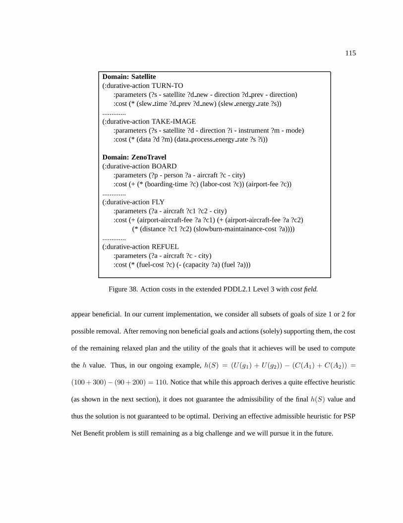
115
Domain: Satellite(:durative-action TURN-TO
:parameters (?s - satellite ?d new - direction ?d prev - direction):cost (* (slew time ?d prev ?d new) (slew energy rate ?s))
.............(:durative-action TAKE-IMAGE
:parameters (?s - satellite ?d - direction ?i - instrument ?m - mode):cost (* (data ?d ?m) (data process energy rate ?s ?i))
Domain: ZenoTravel(:durative-action BOARD
:parameters (?p - person ?a - aircraft ?c - city):cost (+ (* (boarding-time ?c) (labor-cost ?c)) (airport-fee ?c))
.............(:durative-action FLY
:parameters (?a - aircraft ?c1 ?c2 - city):cost (+ (airport-aircraft-fee ?a ?c1) (+ (airport-aircraft-fee ?a ?c2)
(* (distance ?c1 ?c2) (slowburn-maintainance-cost ?a)))).............(:durative-action REFUEL
:parameters (?a - aircraft ?c - city):cost (* (fuel-cost ?c) (- (capacity ?a) (fuel ?a)))
Figure 38. Action costs in the extended PDDL2.1 Level 3 with cost field.
appear beneficial. In our current implementation, we consider all subsets of goals of size 1 or 2 for
possible removal. After removing non beneficial goals and actions (solely) supporting them, the cost
of the remaining relaxed plan and the utility of the goals that it achieves will be used to compute
the h value. Thus, in our ongoing example, h(S) = (U(g1) + U(g2)) − (C(A1) + C(A2)) =
(100 + 300)− (90 +200) = 110. Notice that while this approach derives a quite effective heuristic
(as shown in the next section), it does not guarantee the admissibility of the final h(S) value and
thus the solution is not guaranteed to be optimal. Deriving an effective admissible heuristic for PSP
Net Benefit problem is still remaining as a big challenge and we will pursue it in the future.
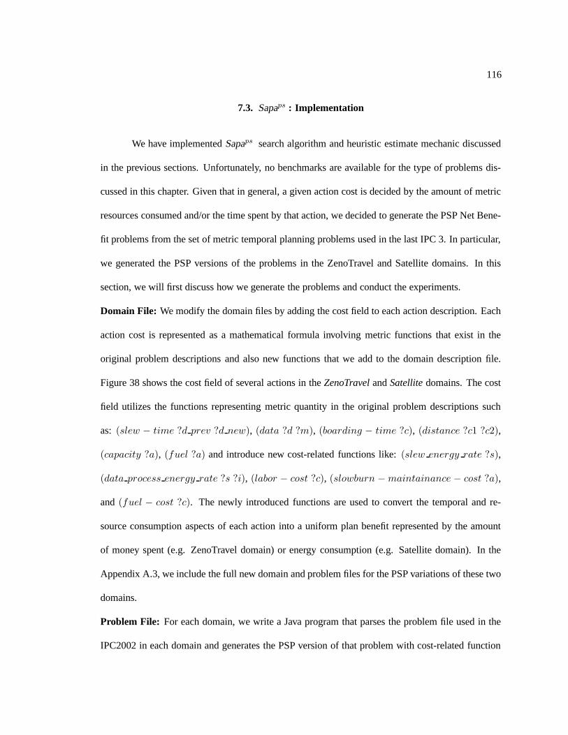
116
7.3. Sapaps : Implementation
We have implemented Sapaps search algorithm and heuristic estimate mechanic discussed
in the previous sections. Unfortunately, no benchmarks are available for the type of problems dis-
cussed in this chapter. Given that in general, a given action cost is decided by the amount of metric
resources consumed and/or the time spent by that action, we decided to generate the PSP Net Bene-
fit problems from the set of metric temporal planning problems used in the last IPC 3. In particular,
we generated the PSP versions of the problems in the ZenoTravel and Satellite domains. In this
section, we will first discuss how we generate the problems and conduct the experiments.
Domain File: We modify the domain files by adding the cost field to each action description. Each
action cost is represented as a mathematical formula involving metric functions that exist in the
original problem descriptions and also new functions that we add to the domain description file.
Figure 38 shows the cost field of several actions in the ZenoTravel and Satellite domains. The cost
field utilizes the functions representing metric quantity in the original problem descriptions such
as: (slew − time ?d prev ?d new), (data ?d ?m), (boarding − time ?c), (distance ?c1 ?c2),
(capacity ?a), (fuel ?a) and introduce new cost-related functions like: (slew energy rate ?s),
(data process energy rate ?s ?i), (labor − cost ?c), (slowburn −maintainance − cost ?a),
and (fuel − cost ?c). The newly introduced functions are used to convert the temporal and re-
source consumption aspects of each action into a uniform plan benefit represented by the amount
of money spent (e.g. ZenoTravel domain) or energy consumption (e.g. Satellite domain). In the
Appendix A.3, we include the full new domain and problem files for the PSP variations of these two
domains.
Problem File: For each domain, we write a Java program that parses the problem file used in the
IPC2002 in each domain and generates the PSP version of that problem with cost-related function
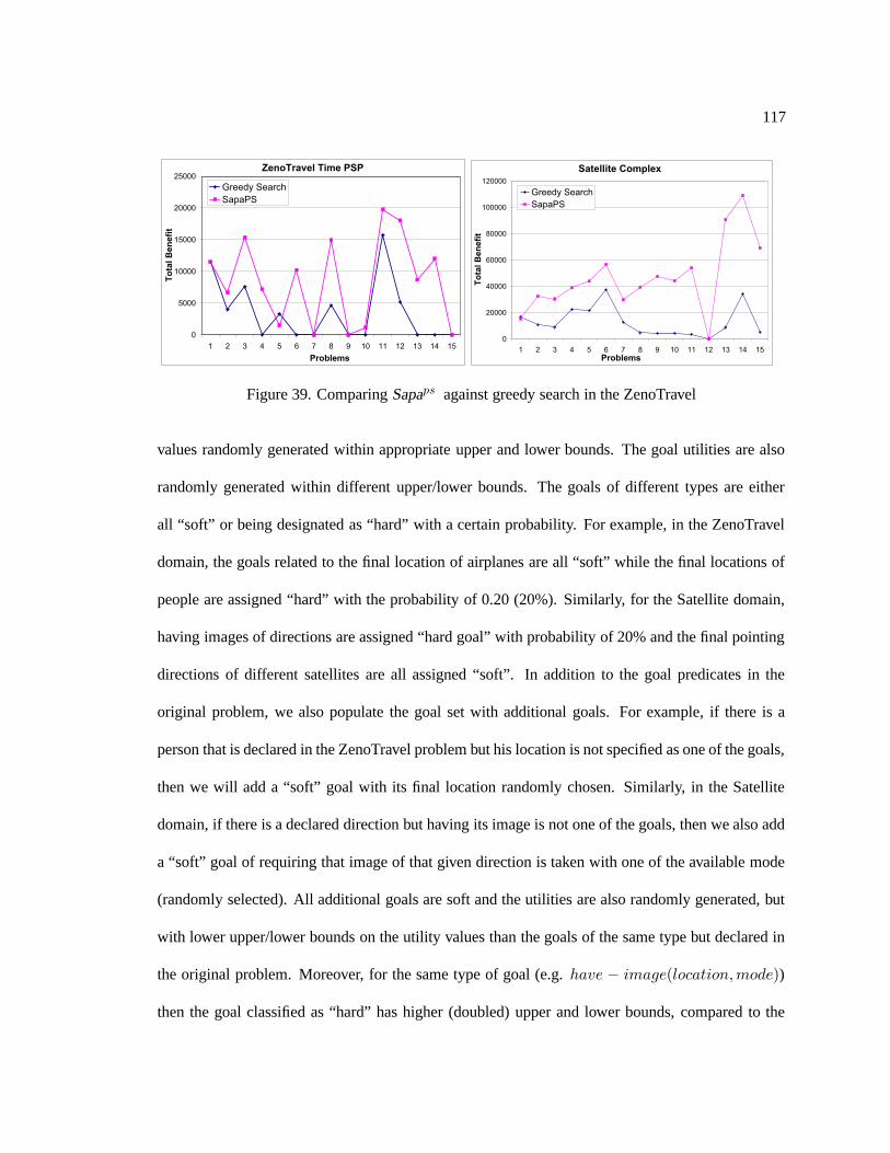
117
ZenoTravel Time PSP
0
5000
10000
15000
20000
25000
1 2 3 4 5 6 7 8 9 10 11 12 13 14 15
Problems
To
tal B
en
efi
t
Greedy Search
SapaPS
Satellite Complex
0
20000
40000
60000
80000
100000
120000
1 2 3 4 5 6 7 8 9 10 11 12 13 14 15 Problems
To
tal B
en
efi
t
Greedy Search
SapaPS
Figure 39. Comparing Sapaps against greedy search in the ZenoTravel
values randomly generated within appropriate upper and lower bounds. The goal utilities are also
randomly generated within different upper/lower bounds. The goals of different types are either
all “soft” or being designated as “hard” with a certain probability. For example, in the ZenoTravel
domain, the goals related to the final location of airplanes are all “soft” while the final locations of
people are assigned “hard” with the probability of 0.20 (20%). Similarly, for the Satellite domain,
having images of directions are assigned “hard goal” with probability of 20% and the final pointing
directions of different satellites are all assigned “soft”. In addition to the goal predicates in the
original problem, we also populate the goal set with additional goals. For example, if there is a
person that is declared in the ZenoTravel problem but his location is not specified as one of the goals,
then we will add a “soft” goal with its final location randomly chosen. Similarly, in the Satellite
domain, if there is a declared direction but having its image is not one of the goals, then we also add
a “soft” goal of requiring that image of that given direction is taken with one of the available mode
(randomly selected). All additional goals are soft and the utilities are also randomly generated, but
with lower upper/lower bounds on the utility values than the goals of the same type but declared in
the original problem. Moreover, for the same type of goal (e.g. have − image(location,mode))
then the goal classified as “hard” has higher (doubled) upper and lower bounds, compared to the
118
“soft” goal of the same type. For example, if the lower and upper bounds of the soft goal of type g
is [1000 − 3000] then the bounds for hard goals of the same type is [2000 − 6000].
Examples of the full domain and problem files for the two domains are presented in the Ap-
pendix A.3. Eventually, we want to use this approach to generate PSP versions of domains/problems
used in the previous International Planning Competitions to create many more benchmarks for test-
ing Sapaps and other PSP solving algorithms.
Greedy Search: To evaluate the Sapaps algorithm, we compare it with a greedy search strategy
on the two domains discussed above. The greedy search algorithm that we implemented is called
“static greedy” because it decides a static order of goals to achieve according to the decreasing order
of goal utilities. Starting from the initial state, we try to first find a lowest cost plan that satisfies all
hard goals. Then, we continuously pick one soft goal at a time and try to find lowest cost plan that
satisfies that single goal and does not delete any of the achieved goals. If there is no plan found that
has less cost than the utility of the goal that it achieves, then we will skip that goal and move on to
the next highest utility goal. This process continues until there is no goal left.
Figure 39 shows the comparisons between the Sapaps ’s algorithm discussed in this chapter
and the greedy search algorithm discussed above for the first 15 problems of the two ZenoTravel
(Time setting) and Satellite (Complex setting) domains. All results were collected using a Pentium
IV 1.4GHz machine with running time limit of 1200 seconds. Both domains and problem sets are
original from the third IPC, and the procedure to make the PSP variations out of them was de-
scribed above. The results show that except for one problem in each domain, the anytime A* search
in Sapaps produces plans which have higher total benefit values than the greedy search. In the
ZenoTravel domain, the average improvement over problems that both approaches can find bene-
ficial solutions is 1.8 times. Moreover, there are 5 instances for which Sapaps can find beneficial
solutions while the greedy approach can not find any. Thus, in those problems, there seem to be
119
no beneficial plan that achieves a single goal but only plans that sharing actions to achieve multiple
goals can be beneficial. For the Satellite domain, the average improvement is 6.1 times. The size
of the plans in the two domains are quite big, with the largest plans found in the Satellite domain
contain around 300 actions.
7.4. Summary and Discussion
In this chapter, we discuss Sapaps , a variation of the Sapa planner, that can handle Partial-
Satisfaction Planning Net Benefit problem. In this type of problem, goals, which can be either
“hard” or “soft”, have different utilities and the plan quality is decided by the tradeoff between the
total achieved goal utility and the total cost of actions in that plan. Sapaps adapts Sapa’s best-first
search and heuristic framework and return “beneficial” solutions in an anytime fashion.
Given that partial satisfaction planning is an area where not much research have been done,
our work discussed in this chapter only scratched the surface and there is a whole range of exciting
problems to tackle. First, there is a variation of the PSP problem involving time-dependent goal
utility for goals with deadline that was discussed by Haddawy & Hanks [38]. The other is the over-
subscription planning problem where there are constraints on the amount of resource, or money
available. This is a variation of PSP Net Benefit that exists in many domains (because it is unrealistic
to assume that the available amount of money or resource is infinite). Even though the Satellite
problems that we tested in Section 7.3 already have this type of constraint, we have not investigated
techniques that specifically deal with them.
Effective heuristic and good state management strategies are important issues in the anytime
best-first search framework of Sapaps (e.g. which explored states to keep and which to discard in
the anytime search framework). For the heuristic part, we want to test the other effective heuristics
such as the one introduced by Smith in the orienting planner [85] or the heuristics using residual
120
cost in AltAltps [88]. The first heuristic seems to be particularly effective for transportation-style
planning domains. To be able to use this type of heuristic in a general domain-independent planner
like Sapaps , besides extending the heuristic, the other possible option is using automatic domain
analysis tool such as TIM [31] to automatically identify problems involving transportation generic
type. Upon discovery, heuristics specialized in this type of problem such as solving the orienting
problem can be used. This approach has shown to be successful in domain-independent planner
such as Hybrid-STAN [30].
The current-heuristic framework in Sapaps for solving PSP problem is also over-dependent
on the cost aspect, even though the goal utility is as important as the action cost in deciding the
overall benefit value of the final plan (and the relaxed plan when evaluating heuristic values). We
plan on investigating backward utility propagation similar to the approach of building the utility
table discussed in [17]. Specifically, we are investigating two approaches of utility propagation
either: (i) offline: one-time as a pre-processing phase; or (ii) oneline: when extracting the relaxed
plan for each state and using only actions and goals involved in the relaxed plan. The backward
propagated utility information can then be combined with the forward-propagated cost functions to
give better overall benefit estimation.
The other interesting problem that we want to tackle is the scenario where there exist de-
pendencies between different action cost or goal utilities. For example, the cost to buy two (left
and right) shoes at a given store may be much smaller than the cost to buy each of them separately.
Moreover, the utility of having a pair of shoes is much higher than having each of them separately.
The current framework of removing “unbeneficial” goals and associated actions in Sapaps can han-
dle the scenarios where goal utilities are pair-wise dependent. However, of bigger subsets of goals,
then other techniques need to be investigated. Besides the inter-dependency relations between dif-
ferent goals, there are other types of goals that may allow partial satisfaction for each individual of

121
them. This is mostly only relevant to metric goals where satisfying a portion of them gives partial
utility value. For example, getting half of the shipment still give some utility more than not getting
anything (but may not be half the utility value of getting the whole shipment). To this end, we are
implementing the “possible metric value” propagation framework over the planning graph building
process and hope that it would give better estimation on what are the estimated incurring cost to
achieve each level of some (goal-related) metric quantity.
CHAPTER 8
Related Work and Discussion
There are various works in planning directly related to the main contributions of this dis-
sertation. These include techniques to handle metric temporal constraints, planning graph based
heuristics, forward state space search management, position-constrained and order-constrained plan
conversion, and partial-satisfaction planning. Even though we have cited many of them in previous
parts of the dissertation, in this chapter we will give a more thorough discussion on their relations
with Sapa and its components.
8.1. Metric Temporal Planning
Although there have been several recent domain-independent heuristic planners for temporal
domains, most of them have been aimed at makespan optimization, ignoring the cost aspects. For
example, both TGP [81] as well as TP4 [39] focus on makespan optimization and ignore the cost
aspects of the plan. As we have argued in this paper, ultimately, metric temporal planners need to
deal with objective functions that are based on both makespan and cost. Nevertheless, the makespan
estimates in both of these planners are better than Sapa because they both reason about mutex
relations between actions and facts. Sapa employs the forward search algorithm and there is no
good way of avoiding the planning graph rebuild procedure for each generated search state. Until
123
now, keeping the cost of building the planning graph minimal by removing the mutex propagation
process seems to be a good strategy (with the price of sacrifycing the makespan-related heuristic
quality). Currently, we have an option in Sapa to use the mutex relations to order the actions in the
extracted relaxed plan and thus improve the heuristic quality. However, the extracted relaxed-plan in
itself may not contains actions that collectively make a good makespan estimation of the real plan.
To improve the makespan estimation, we are currently looking at using only the static mutex in the
graphplan building process and skip the dynamic mutex propagation. However, this approach still
requires reasoning about mutexes explicitly; therefore, we believe that a better approach may be to
first pre-process the binary representation in PDDL and convert it into k-ary representation (SAS+)
using the tool provided by Helmert [40]. This would allow implicit reasoning about mutexes when
building the graph and can give better heuristics without necessarily increasing the planning graph
building cost.
One recent research effort that recognizes the multi-objective nature of planning is the MO-
GRT system [80]. On one hand, the MO-GRT approach is more general than ours in the sense that
it deals with a set of non-combinable quality metrics. The MO-GRT approach however treats time
similar to other consumable resources (with infinite capacity). Temporal constraints on the planning
problems (such as when an effect should occur during the course of action), goal deadlines, or
concurrency are ignored in order to scale down the problem to the classical planning assumptions.
Metric-FF [43] and MIPS [24] are two other forward state space planners that can handle resource
constraints (both of them generate sequential plans). MIPS handles durative actions by putting
in the action durations and post-processing the sequential p.c plans. Our state-space search for
temporal planning algorithm is inspired by the TLPlan [1] in which concurrent durative actions
are allowed in the state representation. Unlike Sapa, TLPlan relies on domain-control knowledge
written in temporal logic to guide its searches. While the approach of simplifying or ignoring
124
some of the temporal constraints while conducting search in MIPS and MO-GRT has advantage
of managing simpler search states and the heuristic estimation routine (and thus can speed up the
planner and reduce memory consumption), the ignorance of temporal aspects of actions can lead
to: (i) lower heuristic quality for objective functions related to time; and (ii) the inability to handle
some types of temporal constraints. For example, it is not clear how the classical-like graphplan can
help derive time-related heuristic estimate. Moreover, it’s not clear how an approach of building
a sequential plan and then post-process to produce concurrent plan later can handle domains such
as the Burn-Match example in the PDDL2.1 manual [28] where actions are forced to execute in
parallel to achieve the goals. This later problem did not show up in the domains used in the IPC-
2002. However, we believe that for a more complicated temporal problems that require those type
of concurrency-forcing constraints and beyond, it is necessary to employ the state representation
similar to TLPlan and Sapa.
Multi-Pegg [101] is another recent planner that considers cost-time tradeoffs in plan gener-
ation. Multi-Pegg is based on the Graphplan approach, and focuses on classical planning problems
with non-uniform cost actions. Multi-Pegg has a unique ability of searching for all possible plans
within a given level limit. This approach is particular useful for the multi-objective problems where
there are multiple non-combinable dimensions in plan quality metrics and thus a pareto set of so-
lution is needed1 . Sapa currently uses a single combined objective function and is not efficiently
engineered for this multi-dimension optimization problem. However, Sapaps is able to find better
quality plans in an anytime fashion and we think that extending this algorithm with some modifica-
tion in node judgment (e.g. beneficial node, termination node) is a good direction to extend Sapa to
handle the pareto-set optimization.
Utilizing the local search framework, ASPEN [14] is another planner that recognizes the
1Nevertheless, like all Graphplan-based planners, the overall plan quality is limited by the number of “levels” in theplanning graph and thus the global best solution is not guaranteed.
125
multi-attribute nature of plan quality. ASPEN advocates an iterative repair approach for planning,
that assumes the availability of a variety of hand-coded plan repair strategies and their characteriza-
tion in terms of their effects on the various dimensions of plan quality. Like ASPEN, LPG [33] is
another planner that employs local search techniques over the action-graph. Unlike ASPEN, LPG
considers domain independent repair strategies that involve planning graph-based modifications.
While the local search strategy seems to be very flexible in dealing with different objective func-
tions and is a good strategy for multi-objective search, some of its drawbacks are the difficulties in
finding global optimum and discovering the insolvability of the problem.
Although we evaluated our cost-sensitive heuristics in the context of Sapa, a forward chain-
ing planner, the heuristics themselves can also be used in other types of planning algorithms. It is
possible due to the fact that directional searches (forward/backward) all need to evaluate the dis-
tances between an initial state and a set of temporal goals. In classical planning, works in [70, 71]
and [98] have shown that heuristics derived from the classical planning graph can help guide back-
ward state space and partial order classical planners effectively. Besides backward search planners,
graphplan-based planners such as TGP can also be made cost-sensitive by propagating the cost func-
tions as part of planning graph expansion phase. These cost functions can then be used as a basis for
variable and value ordering heuristics to guide its backward branch-and-bound search. Given that a
similar approach in graphplan-based search for classical planning has been shown to be successful
in [51], similar approach in metric temporal planning can be promising. Different from the current
strategy in Sapa, for backward search and graphplan-based planners, because we only need to build
the planning graph once, employing additional (most time-consuming) techniques to help improv-
ing the information encoded in the planning graph may be more beneficial. Examples are the more
aggressive use of the mutex information and better cost-propagation techniques (compared to the
simple assumption in the max or sum rules).
126
In the context of other approaches that use planning graphs as the basis for deriving heuristic
estimates such as Graphplan-HSP [51], AltAlt [70], RePOP [71], and FF [41] 2, our contribution
can be seen as providing a way to track cost as a function of time on planning graphs. An interesting
observation is that cost propagation is in some ways inherently more complex than makespan propa-
gation. For example, once a set of literals enter the planning graph (and are not mutually exclusive),
the estimate of the makespan of the shortest plan for achieving them does not change as we continue
to expand the planning graph. In contrast, the estimate of the cost of the cheapest plan for achieving
them can change until the planning graph levels off. This is why we needed to carefully consider
the effect of different criteria for stopping the expansion of the planning graph on the accuracy of
the cost estimates (Section 4.3). Another interesting point is that within classical planning, there
was often a confusion between the notions of cost and makespan. For example, the “length of a
plan in terms of number of actions” can either be seen as a cost measure (if we assume that actions
have unit costs), or a makespan measure (if we assume that the actions have unit durations). These
notions get teased apart naturally in metric temporal domains.
In this dissertation, we concentrated on developing heuristics that can be sensitive to multi-
ple dimensions of plan quality (specifically, makespan and cost). An orthogonal issue in planning
with multiple criteria is how the various dimensions of plan quality should be combined during
optimization. The particular approach we adopted in our empirical evaluation–namely, considering
a linear combination of cost and time–is by no means the only reasonable way. Other approaches
involve non-linear combinations of the quality criteria, as well as “tiered” objective functions (e.g.
rank plans in terms of makespan, breaking ties using cost). A related issue is how to help the user
2Note that there are two different ways of extracting the heuristic values from the planning graph. The first approachused in [70] and [71] estimate heuristic using the “level” information at which goals are achievable and an approach inFF that extract the relaxed plan. The heuristics based on the level information in [70, 71] can not directly be extended touse in temporal planning due to the fact that they assume all goals appear at the same time/level. The second approachof extracting the relaxed plan is more flexible and does not make such an assumption. Moreover, the relaxed-planbased heuristics work with an actual set of actions and thus is open for various techniques of adjustment for heuristicimprovement (e.g. mutex, add/remove actions).
127
decide the “weights” or “tiers” of the different criteria. Often the users may not be able to articulate
their preferences between the various quality dimensions in terms of precise weights. A more stan-
dard way out of this dilemma involves generating all non-dominated or Pareto-optimal plans3 , and
presenting them to the user. Unfortunately, often the set of non-dominated plans can be exponential
[73]. The users are then expected to pick the plan that is most palatable to them. Unfortunately,
the users may not actually be able to judge the relative desirability of plans when the problems are
complex and the plans are long. Thus, a more practical approach may involve resorting to other
indirect methods such as preference elicitation techniques [13, 92].
8.2. Partialization
The complementary tradeoffs provided by the p.c. and o.c. plans have been recognized
in classical planning. One of the earliest efforts in attempt to improve the temporal flexibility of
plans was the work by Fade and Regnier [26] who discussed an approach for removing redundant
orderings from the plans generated by STRIPS system. Later work by Mooney [66] and Kamb-
hampati & Kedar [49]characterized this partialization process as one of explanation-based order
generalization. These works assume STRIPS representation with-non durative action, our approach
works for metric temporal plans where there are substantially more complicated set of constraints
and a large set of useful objective functions for the partialization process. Moreover, the work in
[90] and [49] can be seen as providing a greedy value ordering strategy over the partialization en-
coding for classical plans. In [90], the value ordering for each SpA is set to the latest action A′ that
gives p and is positioned before A in the original t.o plan. In [49], the value ordering is improved
by choosing the earliest consistent supporter ordered according to the original t.o plan instead of
the latest one. Compare with the previous approach, the new ordering can lead to equal or better
3A plan P is said to be dominated by P ′ if the quality of P ′ is strictly superior to that of P in at least one dimension,and is better or equal in all other dimensions [16, 73].
128
quality plan in terms of makespan if applied to the same sequential plan. Regardless of the variable
ordering, the greedy value ordering in the two approaches discussed above will lead to linear-time
backtrack-free algorithms to find a consistent o.c. plan. The orderings are based on the total order-
ing between actions in the original p.c. plan and is insensitive to any objective function and thus
do not guarantee the solution is optimal in term of any objective function discussed in the litera-
ture. Nevertheless, while the greedy strategy in [49] is geared toward the optimization criterion of
minimizing the parallel level of the final o.c plan, our greedy technique is aimed toward minimizing
plan with smaller makespan. Unlike the strategies we presented in Sections 6.3, all previous value
ordering strategies in greedy searches assume the starting p.c plan is sequential and actions are in-
stantaneous. Therefore, there is only one ordering between a given pair of action while there can
be multiple orderings representing different temporal relations between a given pair of actions in
our approaches. The recent work by Winner & Veloso [96] extended the de-ordering techniques in
[90] to planning problems with conditional effects. This is done by building the need tree to capture
the possible supporting list. The final plan is built greedily using the need tree and also does not
guarantee any optimality. More recent de-ordering techniques are the post-processing routine used
in the MIPS planner [25] and the “push-up” techniques used in the AltAltP planner [72] to produce
parallel plans. There is not much difference between the post-processing approach in MIPS and the
greedy partialization routine in Sapa except that MIPS assumes a sequential plan while Sapa pro-
duces parallel plans. In AltAltP, the “push-up” technique is used “online” instead of “off-line” and
is invoked whenever a new action is added to the partial plan. Because it’s done online, this can help
improve the heuristic estimation regarding the makespan value and thus improve the parallelism of
the final plan. In Sapa, even though the partial plan is parallel and thus gives an adequate g value,
the experimental results in Section 6.5 show that the starting time of those parallel actions can be
pushed earlier to give a better indication of the makespan of the partial plan (g value). Therefore,
129
variation of the “push-up” technique in AltAltP can potentially used in Sapa to improve this part of
the heuristic estimate.
Backstrom [2] categorized approaches for partialization into “de-ordering” approaches and
“re-ordering” approaches. Both of them assume the seed plan to be sequential. The order gener-
alization algorithms discussed above fall under the de-ordering category. He was also the first to
point out the NP-hardness of maximal partialization with the objective function of minimizing the
number of orderings and to characterize the previous algorithms as greedy approaches. The greedy
algorithm discussed in Section 6.3, while working for both sequential and parallel plans, can be cate-
gorized as “de-ordering” according to Backstrom’s [2] criteria because it makes use of the temporal
orderings between actions in the seed p.c plan. Setting up the CSOP encoding (Section 6.2) and
solving it to optimality (Section 6.4) encompasses both de-ordering and re-ordering partialization–
based on whether or not we include the optional constraints to make the orderings on Poc consistent
with Ppc. However, while the “de-ordering” and “re-ordering” algorithms are only discussed for
classical planning problems, both greedy and optimal techniques discussed in this thesis work for
both the sequential and parallel plans and for a more complex problems involving both temporal and
metric resource constraints. Moreover, while only one polynomial algorithm for the easiest class of
minimal de-ordering is presented in [2], we provide several algorithms to build the o.c. plans with
different criteria. It’s also interesting to note that while there are several implemented variations of
the greedy de-ordering technique, there was no implementation of the re-ordering problem. To our
knowledge, we are the first to have actually implemented an optimal partialization technique that
encompasses the re-ordering scenario.
It is interesting to note that our encoding for partialization is closely related to the so-called
“causal encodings” [52]. Unlike causal encodings, which need to consider supporting a precondi-
tion or goal with every possible action in the action library, the partialization encodings only need
130
to consider the actions that are present in Ppc. In this sense, they are similar to the encodings for
replanning and plan reuse described in [65]. Also, unlike causal encodings, the encodings for par-
tialization demand optimizing rather than satisficing solutions. Finally, in contrast to our encodings
for partialization which specifically handle metric temporal plans, causal encodings in [52] are lim-
ited to classical domains. In the same line of work, the recent work by Vidal & Geffner [91] captures
the causal relationship of actions in temporal planning. This CSP encoding when solved will return
an optimal makespan canonical plan where each ground action instance can appear at most once.
This encoding shows a lot of similarity with our CSOP encoding discussed in Section 6.2. They are
mostly different in the set of actions involved in the encoding and the way the CSOP encoding is
solved. While we convert it into the MILP encoding and solve it to optimality using an off-the-shelf
solver, Vidal & Geffer [91] use an CSOP branch and bound solver with fine-tuned variable and value
orderings for this particular type of encoding. Moreover, they only capture temporal constraints and
cannot handle metric constraints.
In scheduling, building the CSP encoding to capture the orderings between tasks is a com-
mon approach [11, 12]. However, unlike planning where the causal relations between actions are
the most critical, most of the constraints in scheduling capture only the resource contention ordering
relations. Those constraints are in some sense similar to the resource mutex constraints discussed
in Section 6.2. Nevertheless, this problem has been more thoroughly investigated in scheduling so
it would be interesting to see how they can be used in the partialization problem in planning to help
give better encoding for resource-related constraints.
8.3. Partial Satisfaction (Over-Subscription) Problem
As we mentioned earlier, there has been very little work on PSP in planning. One possible
exception is the PYRRHUS planning system [95] which considers an interesting variant of the
131
partial satisfaction planning problem. In PYRRHUS, the quality of the plans is measured by the
utilities of the goals and the amount of resources consumed. Utilities of goals decrease if they are
achieved later than the goals’ deadlines. Unlike the PSP problem discussed in this dissertation, all
the logical goals still need to be achieved by PYRRHUS for the plan to be valid. Haddawy & Hanks
[38] extended the work in [95] to a more expressive goal utility model where partial satisfaction of
individual goals is discussed. Moreover, besides achievable goals with deadlines, handling of goals
of maintainance is also discussed. While independence is assumed for different goals’ utilities and
also the attributes in each goal’s utility model, it would be interesting to extend the PSP model to
consider utility dependency between the set of individual goals (e.g. utility of the left and right
shoes). While the theoretical discussions in PYRRHUS concern many important issues in partial
satisfaction planning problems, the implementation is domain dependent and do not seem to be able
to scale up well. We are extending the domain independent technique in Sapaps to handle several
issues discussed in PYRRHUS, especially the time-dependent goal utility issue.
The first domain-independent heuristic planner that solves a partial satisfaction planning
problem is the Maxp planner, which is a variation of TP4 [39]. Given a time limit, Maxp finds
the maximal (biggest size) subset of goals that can be achieved. This is a (stripped down) varia-
tion of the PSP Net Benefit where goal utilities are much higher than action costs and there exist a
planner’s running time limit. More recently, Smith [84] motivated the over-subscription problems
in terms of their applicability to the NASA planning problems. On one hand, it is different from
the PSP Net Benefit problem described in Chapter 7, the motivated problems belong to a variation
where not all the goals can be achieved due to the limitation on resources. On the other hand, the
randomly generated Satellite problems discussed in Sapaps ’s empirical result section (Section 7.3)
also have resource limitation constraints (each satellite has limited data-storage) and thus in some
sense encompass the resource-limited PSP variation. Smith ([85]) also proposed a planner for over-
132
subscription planning problems of this type in which the solution of the abstracted planning prob-
lem is used heuristically to select the subset of goals and the orders to achieve them. The abstract
planning problem is built by propagating the cost on the planning graph and constructing the orien-
teering (a variation of prize-collecting traveling salesman) problem. The subset of goals and their
orderings are then found from solving this orienting problem and are used to guide a POCL plan-
ner. By heuristically selecting a subset of goals up front and commit to satisfy all goals in this
set while neglecting the other, this approach is similar to the AltAltps planner discussed in [89].
The main difference between them is that the orienteering problem needs to be constructed using
domain-knowledge for different planning domains while AltAltps relies on the domain-independent
heuristic based on cost propagation on the planning graph. The other difference is that solving the
orienteering problems also provides a partial order between goals. This set of orderings can help
significantly simplify the planning task given to the base POCL planner. While both orienteering
planner [85] and AltAltps [89] heuristically select the subset of goals up-front, Sapaps does not
make such commitment and thus it can potentially correct the set of beneficial goals as it searches
deeper and goes closer to the goals. Nevertheless, the sophisticated heuristic estimation approach
used in those two planners can be used in Sapa to evaluate and rank each search node in the queue.
In particular, the orienting solution can be a very good heuristic estimate in “transportation” prob-
lems, which is the most common type among planning benchmarks. In [85], Smith discussed the
problem where solution for the orienting problem in itself does not give a good heuristic estimate
and thus it is necessary to solve it repeatedly. It would be better then to employ the solving of
the orienting problem as a heuristic routine in Sapaps ’s current anytime A* search to avoid being
over-dependent on the quality of a single solution to the orienting problem.
Besides the heuristic search, there are several other approaches that can solve the PSP Net
Benefit problems to optimal. In [89], van den Briel et. al. introduced OptiPlan planner, which
133
encodes the k-level planning graph using Mixed Integer Linear Programming (MILP) encoding.
The PSP Net Benefit specifications (action cost and goal utility) are represented by suitable objective
function. While this approach can find optimal solution with upper-bound constraint on the total
parallel length of the final plan, there is no easy way to extend it to find the global optimal solution
for the PSP Net Benefit problem. Regarding this issue, it seems that encoding the PSP problem as
deterministic Markov Decision Process (MDP) [8] can help finding optimal solutions for PSP Net
Benefit problems. Nevertheless, given the scaling up problem of MDP representation (compared to
heuristic search), it is not clear how this approach compares to the performance of Sapaps using
admissible heuristics.
Over-subscription issues have received relatively more attention in the scheduling commu-
nity. Earlier work in scheduling over-subscription used greedy approaches, in which tasks of higher
priorities are scheduled first [56, 78]. More recent efforts have used stochastic greedy search algo-
rithms on constraint-based intervals [32], genetic algorithms [34], and iterative repairing technique
[58] to solve this problem more effectively. Specifically, the last two approaches try to find better
quality schedules after the first consistent schedule is found. Again, stochastic approach has advan-
tage of easier adaptation to a new objective function, but also has a drawback of not guaranteeing
the global optimality.
CHAPTER 9
Conclusion and Future Work
9.1. Summary
The work presented in this dissertation seeks the development of a scalable domain-
independent planner that can handle a variety of metric and temporal constraints. This quest for an
effective metric temporal planner is motivated from the practical necessity: while many real-world
applications involve various temporal constraints and require the handling of continuous variables,
previous metric temporal planners mostly relied on domain-control knowledge to scale up.
Sapa, which is the centerpiece of this dissertation, is a domain-independent heuristic forward
chaining planner that can handle durative actions, metric resource constraints, and deadline goals.
It extends many recent advances in classical planning such as reachability analysis and heuristic
estimates based on relaxed planning assumption, and it is also designed to be capable of handling
the multi-objective nature of the metric temporal planning. The three main interrelated contributions
to metric temporal planning of this dissertation are:
• A temporal planning-graph based method for deriving multi-objective heuristics that are sen-
sitive to both cost and makespan and an easy way of adjusting the heuristic estimates to take
the metric resource limitations into account. The heuristics then can be used to effectively
guide the forward state-space temporal planner.
135
• Greedy/optimal partialization routines that can be used to post-process the position-
constrained plans to improve their execution flexibility.
• The adaptation of the search algorithm and heuristic in Sapa to solve Partial Satisfaction
Planning problems where, goals, either “hard” or “soft”, have different utilities and the plan
quality is measured by the tradeoff between the total achieved goal utility and total cost of
actions in the plan.
We described the technical details of the search algorithm and the three main contributions
listed above. We also presented the empirical evaluations of the current implementation of Sapa,
the partialization software, and the Sapaps planner.
9.2. Future Work
While the current implementations of Sapa and Sapaps planners perform well on the highest
expressive level for metric temporal planning in the IPC3, there are still many places where improve-
ments can be made. In Section 3.3, 4.6, 6.6, and 7.4, we have discussed the potential extensions
to different aspects of the planners such as expressiveness or heuristic quality. The most important
topics are: (i) supporting more expressive metric temporal constraints such as continuous change
and exogenous event; (ii) supporting more complicated formulas for action cost and goal utility
(e.g. action costs and goal utilities that change according to action-execution and goal-achievement
time); (iii) improving heuristic estimate for multi-objective search.
Nonetheless, metric temporal constraints, while important, are not always the only con-
straints involved in the real-world applications for planning. There are other important issues such
as probability, contingency, and sensing. Even though there have been a lot of work in planning
to deal with them, most of them concern the scenarios where no metric or temporal constraints
136
are involved. Thus, in the future, we plan to investigate effective ways to search for high quality
plan in the presence of both uncertainty and metric temporal constraints. Given that forward state
space search has shown to be a good option for conformant and contingent planning, combining the
techniques in forward state-space metric temporal planning and contingent planning is a promising
direction. For probabilistic setting, recent work by Younes & Simmons [100] provides a framework
for generating probabilistic concurrent plan (policy) with continous time by simplifying each step
to a normal PDDL2.1 durative actions. It would be interesting to see how we can adapt the current
forward search algorithm into this scenario where concurrent temporal plan is required, but the final
plan should still have a high probability of success.
REFERENCES
[1] Bacchus, F. & Ady, M. 2001. Planning with Resources and Concurrency: A Forward Chaining
Approach. In Proc. of Seventeenth International Joint Conference on Artificial Intelligence.
[2] Backstrom, C. 1998. Computational Aspects of Reordering Plans. In Journal of Artificial
Intelligence Research 9, 99-137.
[3] Beck, C. and Fox, M. 1998. A Generic Framework for Constraint-Directed Search and Schedul-
ing. In Artificial Intelligence Magazine.
[4] Blum, A. and Furst, M. 1995. Fast planning throught planning graph analysis. In Proc. of
Fourteenth International Joint Conference on Artificial Intelligence (IJCAI).
[5] Blum, A. and Furst, M. 1997. Fast planning throught planning graph analysis. In Artificial
Intelligence 90:281–300, 1997.
[6] Blum, A. and Langford, J. 1999. Probabilistic Planning in the Graphplan Framework. In
European Conference in Planning
[7] Bonet, B., Loerincs, G., and Geffner, H. 1997. A robust and fast action selection mechanism
for planning. In Proc. of Fourteenth National Conference on Artificial Intelligence (AAAI)
[8] Boutilier, C., Dean, T., and Hanks, S. 1999. Decision-Theoretic Planning: Structural As-
138
sumptions and Computational Leverage. In Journal of Artificial Intelligence Research (JAIR),
11 (p.1-94)
[9] Bresina, J., Dearden, R., Meuleu, N, Ramakrishnan, S., Smith, D., and Washington, R. 2002.
Planning under Continuous Time and Resource Uncertainty: A Challenge for AI. Workshop ??
in UAI-02.
[10] Bryce, D., Kambhampati, S. and Smith, D. 2004. Planning in Belief Space with a Labelled
Uncertainty Graph In AAAI 2004 workshop on Learning and Planning in Markov Decision
Processes.
[11] Cesta, A., Oddi, A. and Smith, S.F. 1998. Profile Based Algorithms to Solve Multiple Capac-
itated Metric Scheduling Problems In Proceedings of the Fourth Int. Conf. on Artificial Intelli-
gence Planning Systems (AIPS-98)
[12] Cesta, A., Oddi, A. and Smith, S.F. 2002. A Constrained-Based Method for Project Scheduling
with Time Windows In Journal of Heuristics (8), p.109-136
[13] Chajewska, U., Getoor, L., Norman, J. and Shahar, Y. 1998. Utility Elicitation as a Classifica-
tion Problem. In Proc. of Fourteenth Uncertainty in Artificial Intelligence Conference.
[14] Chien,S., Rabideau, Knight,R., Sherwood,R., Engelhardt,B., Mutz, D., Estlin, T., Smith, B.,
Fisher, F., Barrett, T., Stebbins, G., Tran, D., 2000. ASPEN - Automating Space Mission
Operations using Automated Planning and Scheduling. In Proc. of SpaceOps-2000
[15] Currie, K., and Tate, A. 1991. O-Plan: the Open Planning Architecture. In Artificial Intelli-
gence Vol. 52, pp 49-86, 1991
[16] Dasgupta, P., Chakrabarti, P.P., and DeSarkar, S. 2001. Multiobjective Heuristic Search.
Vieweg & Son/Morgan Kaufmann.
139
[17] Dearden, R., Meuleau, N., Ramakrishnan, S., Smith, D., and Washington, R. 2003. Incremen-
tal Contingency Planning. In ICAPS-03 Workshop on Planning under Uncertainty.
[18] Dechter, R., Meiri, I., and Pearl, J. 1990. Temporal Constraint Network. In Artificial Intelli-
gence Journal 49.
[19] Do, M. and Kambhampati, S. 2001. Sapa: A domain independent heuristic metric temporal
planner. In Proc. of Sixth European Conference on Planning
[20] Do, M., and Kambhampati, S. 2002. Planning graph-based heuristics for cost-sensitive tem-
poral planning. In Proc. of Sixth International Conference on Artificial Intelligence Planning
and Scheduling.
[21] Do, M. and Kambhampati, S. 2003. Improving the Temporal Flexibility of Position Con-
strained Metric Temporal Planning. In Proc. of Thirteenth International Conference on Artificial
Intelligence Planning and Scheduling.
[22] Do, M. and Kambhampati, S. 2003. Sapa: a multi-objective metric temporal planer. In Journal
of Artificial Intelligence Research 20 (p.155-194)
[23] Do, M., and Kambhampati, S. 2004. Planning and Scheduling Connections through Exoge-
nous Events. In Integrating Planning into Scheduling Workshop, ICAPS04
[24] Edelkamp, S. 2001. First Solutions to PDDL+ Planning Problems In PlanSIG Workshop.
[25] Edelkamp, S. 2003. Taming numbers and durations in the model checking integrated planning
system. In Journal of Artificial Intelligence Research 20 (p.195-238)
[26] Fade, B. and Regnier, P. 1990 Temporal Optimization of Linear Plans of Action: A Strategy
Based on a Complete Method for the Determination of Parallelism Technical Report
140
[27] Fox, M. and Long, D. 2002. Third International Planning Competition.
http://www.dur.ac.uk/d.p.long/competition.html
[28] Fox, M. and Long, D. 2001. PDDL2.1: An Extension to PDDL for Expressing Temporal
Planning Domains. In Journal of Artificial Intelligence Research.
[29] Fox, M. and Long, D. 2001. PDDL+: Planning with time and metric resources. Technical
Report, University of Durham.
[30] Fox, M. and Long, D. 2001. Hybrid STAN: Identifying and Managing Combinatorial Optimi-
sation Sub-problems in Planning. In Proceedings of IJCAI.
[31] Fox, M. and Long, D. 1998. The Automatic Inference of State Invariants in TIM. In Journal
of AI Research. vol. 9. pp. 367-421.
[32] Frank, J.; Jonsson, A.; Morris, R.; and Smith, D. 2001. Planning and scheduling for fleets of
earth observing satellites. In Sixth Int. Symp. on Artificial Intelligence, Robotics, Automation &
Space.
[33] Gerevini, A. and Serina, I. 2002. LPG: A Planner Based on Local Search for Planning Graphs.
In Proc. of Sixth International Conference on Artificial Planning and Scheduling (AIPS-02)
[34] Globus, A.; Crawford, J.; Lohn, J.; and Pryor, A. 2003. Scheduling earth observing sateliites
with evolutionary algorithms. In Proc. Int. Conf. on Space Mission Challenges for Infor. Tech..
[35] Garrido, A., Onaindia, E., and Barber, F. 2001. Time-optimal planning in temporal problems.
In Proc. of European Conference on Planning (ECP-01).
[36] Garland, A. and Lesh, N. 2002 Plan Evaluation with Incomplete Action Descriptions In Proc.
of 14th National Conference in Artificial Intelligence.
141
[37] Ghallab, M. and Laruelle, H. 1994. Representation and control in IxTeT, a temporal planner.
In Proc. of Second International Conference on Artificial Intelligence Planning and Scheduling
[38] Haddawy, P., & Hanks S. 1998. Utility Models for Goal-Directed, Decision-Theoretic Plan-
ners. In Computational Intelligence 14(3)
[39] Haslum, P. and Geffner, H. 2001. Heuristic Planning with Time and Resources In Proc. of
Sixth European Conference on Planning
[40] Helmert, M. 2004. A Planning Heuristic Based on Causal Planning Analysis. In Proc. of
ICAPS.
[41] Hoffmann, J. & Nebel, B. 2001. The FF Planning System: Fast Plan Generation through
Heuristic Search. In Journal of Artificial Intelligence Research 14:253-302.
[42] Hoffman, J. and Nebel, B. 2001. RIFO Revisited: Detecting Relaxed Irrelevance. In Proc. of
6th European Conference on Planning.
[43] Hoffmann, J. 2002. Extending FF to Numerical State Variables. In Proc. of 15th European
Conference on Artificial Intelligence.
[44] Hoffmann, J. 2000. http://www.informatik.uni-freiburg.de/ hoffmann/ff.html
[45] Ihrig, L., Kambhampati, S. Design and Implementation of a Replay Framework based on a
Partial order Planner. Proc. AAAI-96.
[46] ILOG Solver Suite. http://www.ilog.com/products/solver/
[47] Kambhampati, S. 1997. Refinement planning as a unifying framework for plan synthesis In
AI Magazine, Vol 18. No. 2
[48] Kambhampati, S. 2003. Classnote of CSE 471/598: Introduction to Artificial Intelligence.
142
[49] Kambhampati, S. & Kedar, S. 1994. An unified framework for explanation-based general-
ization of partially ordered and partially instantiated plans. In Artificial Intelligence Journal 67,
29-70.
[50] S. Kambhampati, E. Lambrecht, and E. Parker 1997. Understanding and Extending Graphplan.
In Fourth European Conference in Planning (ECP-97)
[51] Kambhampati, S. and Nigenda, R. 2000. Distance based goal ordering heuristics for Graph-
plan. In Proc. of Fifth International Conference on Artificial Intelligence Planning and Schedul-
ing.
[52] Kautz, H., McAllester, D. and Selman B. Encoding Plans in Propositional Logic In Proc.
KR-96.
[53] Koehler, J. 1998. Planning under Resource Constraints. In Proc. of Eleventh European
Conference on Artificial Intelligence
[54] J. Koehler, B. Nebel, J. Hoffmann, Y. Dimopoulos. Extending Planning Graphs to an ADL
Subset In Proc. of European Conference in Planning.
[55] Koehler, J. and Hoffman J. 2000. On Reasonable and Forced Goal Orderings and their Use
in an Agenda-Driven Planning Algorithm. In Journal of Artificial Intelligence Research, Volumn
12.
[56] Kramer, L. and Giuliano, M. 1997. Reasoning About and Scheduling Linked HST Observa-
tions with Spike. In Proc. of Int. Workshop on Planning and Scheduling for Space.
[57] Kramer, L. 2000. Generating a Long Range Plan for a new Class of Astronomical Observato-
ries. In Proc. of 2nd NASA Workshop on Planning and Scheduling for Space.
143
[58] Kramer, L. A., and Smith, S. 2003. Maximizing flexibility: A retraction heuristic for oversub-
scribed scheduling problems. In Proc. of IJCAI-03.
[59] Laborie, P. and Ghallab, M. Planning with sharable resource constraints. In Proc. of Fourteenth
International Joint Conference on Artificial Intelligence (IJCAI).
[60] Lifschitz, E. 1986. On the semantics of STRIPS. In Proc. of 1986 Workshop: Reasoning
about Actions and Plans.
[61] Long, D. and Fox, M. 1998 Efficient Implementation of the Plan Graph in STAN. In Journal
of AI Research (JAIR), Volume 10, pages 87-115.
[62] Long, D. and Fox, M. 2003. The 3rd International Planning Competition: results and analysis
In Journal of Artificial Intelligence Research 20 (p.1-59).
[63] McDermott, D. & the AIPS98 planning competition committee (1998). 1998.
PDDL - The Planning Domain Description Language. Technical Report. Available at
www.cs.yale.edu/homes/dvm.
[64] McDermott, D. 2003. Reasoning about autonomous processes in an estimated-regression
planner. In Proc. Int’l. Conf. on Automated Planning and Scheduling.
[65] Mali, A. Plan Merging and Plan Reuse as Satisfiability Proc ECP-99.
[66] Mooney, R. J. Generalizing the Order of Operators in Macro-Operators Proc. ICML-1988
[67] Morris, P. and Muscettola, N. 2000. Execution of Temporal Plans with Uncertainty. In Proc.
of 12th National Conference on Artificial Intelligence (AAAI).
[68] Muscettola, N. 1994. Integrating planning and scheduling. Intelligent Scheduling.
144
[69] Nebel, B., Dimopoulos, Y. and Koehler, J. 1997. Ignoring Irrelevant Fact and Operators in
Plan Generation. In Proc. of Fourth European Conference on Planning.
[70] Nguyen, X., Kambhampati, S., and Nigenda, R. 2001. Planning Graph as the Basis for
deriving Heuristics for Plan Synthesis by State Space and CSP Search. In Artificial Intelligence
Journal.
[71] Nguyen, X., and Kambhampati, S., 2001. Reviving Partial Order Plan In Proc. of Seventeenth
International Joint Conference on Artificial Intelligence (IJCAI).
[72] Nigenda, R., and Kambhampati, S., 2002. AltAlt-P: Online Partialization of Plans with
Heuristic Search. In Journal of Artificial Intelligence Research 19 (p.631–657).
[73] Papadimitriou C. H. and Yannakakis M. Multiobjective Qury Optimization. ACM Conference
on Principles of Database Systems (PODS) 2001.
[74] Pednault, E.P.D. 1988. Synthesizing plans that contain actions ith context-dependent effects.
In Comput. Intell. 4
[75] Penberthy, S. and Well, D. 1994. Temporal Planning with Continuous Change. In Proc. of
11th National Conference on Artificial Intelligence (AAAI).
[76] Pinedo, M. 1995. Scheduling: Theory, Algorithms, and Systems. Prentice Hall
[77] Porteous, J., Sebastia, L., Hoffmann, J. 2001. On the Extraction, Ordering, and Usage of
Landmarks in Planning. In Proc. of the 6th European Conference on Planning.
[78] Potter, W. and Gasch, J. 1998. A Photo Album of Earth: Scheduling Landsat 7 Mission Daily
Activities. In Proc. of SpaceOps.
145
[79] Refanidis, I. and Vlahavas, I. 2001. The GRT Planner: Backward Heuristic Construction in
Forward State Space Planning. Journal of Artificial Intelligence Research, 15.p:115-161.
[80] Refanidis, I. and Vlahavas, I. 2001. A Framework for Multi-Criteria Plan Evaluation in
Heuristic State-Space Planning Workshop on Planning with Resources, IJCAI-01.
[81] Smith, D. and Weld, D. 1999. Temporal Planning with Mutual Exclusion Reasoning. In Proc.
of 16th International Joint Conference on Artificial Intelligence (IJCAI)
[82] Smith, D. and Weld, D. 1998. Conformant Graphplan In National Conference In Artificial
Intelligence (AAAI)
[83] Smith, D., Frank J., and Jonsson A. 2000. Bridging the gap between planning and scheduling.
The Knowledge Engineering Review, Vol. 15:1.
[84] Smith, D. 2003. The Mystery Talk. Plannet Summer School
[85] Smith, D. 2004. Choosing Objectives in Over-Subscription Planning. In Proc. of ICAPS-04.
[86] Srivastava, B., Kambhampati, S., and Do, M. 2001. Planning the Project Management Way:
Efficient Planning by Effective Integration of Causal and Resource Reasoning in RealPlan. Arti-
ficial Intelligence Journal 131.
[87] Tsamardinos, I., Muscettola, N. and Morris, P. Fast Transformation of Temporal Plans for
Efficient Execution. In Proc. 15th National Conference on Artificial Intelligence (AAAI).
[88] van den Briel, M., Sanchez, R., Kambhampati, S. 2004. Effective Approaches for Partial
Satisfaction (Over-Subscription) Planning. In Proc. of Workshop on Integrating Planning into
Scheduling, ICAPS04.
146
[89] van den Briel, M., Sanchez, R., Do, M., Kambhampati, S. 2004. Effective Approaches for Par-
tial Satisfaction (Over-Subscription) Planning. In Proc. of 19th National Conference on Artificial
Intelligence (AAAI04).
[90] Veloso, M., Perez, M, & Carbonell, J. 1990. Nonlinear planning with parallel resource allo-
cation. In Workshop on Innovative Approaches to Planning, Scheduling and Control.
[91] Vidal, V., & Geffner, H. 2004. Branching and Pruning: An Optimal Temporal POCL Planner
based on Constraint Programming. In Proceedings of the Nineteenth National Conference on
Artificial Intelligence (AAAI-2004)
[92] Vu, H., & Haddawy 2003. Similarity of Personal Preferences: Theoretical Foundations and
Empirical Analysis. In Artificial Intelligence ??, p.??-??
[93] Weld, D., Anderson, C., and Smith, D. 1998. Extending Graphplan to Handle Uncertainty and
Sensing Actions. In Proceedings of AAAI ’98.
[94] Weld, D. 1999. Recent advances in Planning. In Artificial Intelligence Magazine
[95] Williamson, M., and Hanks, S. 1994. Optimal Planning with a Goal-Directed Utility Model.
In Proc. of AIPS-94.
[96] Winner, E. and Veloso, M. Analyzing Plans with Conditional Effects In Proc. of 6th Interna-
tional Conference on Artificial Intelligence Planning and Scheduling.
[97] Wolfman, S. and Weld, D. 1999. The LPSAT system and its Application to Resource Planning.
In Proc. of 16th International Joint Conference on Artificial Intelligence.
[98] Younes, H. and Simmons, R. 2003. VHPOP: Versatile heuristic partial order planner. In
Journal of Artificial Intelligence Research 20
147
[99] Younces, H. 2003. Extending PDDL to model stochastic decision process. In Workshop on
PDDL, ICAPS-2003.
[100] Younces, H. and Simmons, R. 2004. Policy Generation for Continous-time Stochastic Do-
mains with Concurrency. In International Conference on AI Planning and Scheduling, ICAPS-
2004.
[101] Zimmerman, T. 2002. Generating parallel plans satisfying multiple criteria in anytime fash-
ion. In Workshop on Planning and Scheduling with Multiple criteria, AIPS-2002

APPENDIX A
Planning Domain and Problem Representation
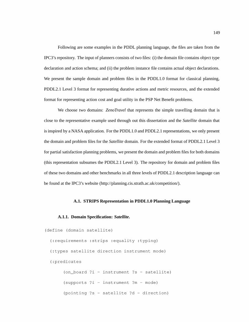
149
Following are some examples in the PDDL planning language, the files are taken from the
IPC3’s repository. The input of planners consists of two files: (i) the domain file contains object type
declaration and action schema; and (ii) the problem instance file contains actual object declarations.
We present the sample domain and problem files in the PDDL1.0 format for classical planning,
PDDL2.1 Level 3 format for representing durative actions and metric resources, and the extended
format for representing action cost and goal utility in the PSP Net Benefit problems.
We choose two domains: ZenoTravel that represents the simple travelling domain that is
close to the representative example used through out this dissertation and the Satellite domain that
is inspired by a NASA application. For the PDDL1.0 and PDDL2.1 representations, we only present
the domain and problem files for the Satellite domain. For the extended format of PDDL2.1 Level 3
for partial satisfaction planning problems, we present the domain and problem files for both domains
(this representation subsumes the PDDL2.1 Level 3). The repository for domain and problem files
of these two domains and other benchmarks in all three levels of PDDL2.1 description language can
be found at the IPC3’s website (http://planning.cis.strath.ac.uk/competition/).
A.1. STRIPS Representation in PDDL1.0 Planning Language
A.1.1. Domain Specification: Satellite.
(define (domain satellite)
(:requirements :strips :equality :typing)
(:types satellite direction instrument mode)
(:predicates
(on_board ?i - instrument ?s - satellite)
(supports ?i - instrument ?m - mode)
(pointing ?s - satellite ?d - direction)
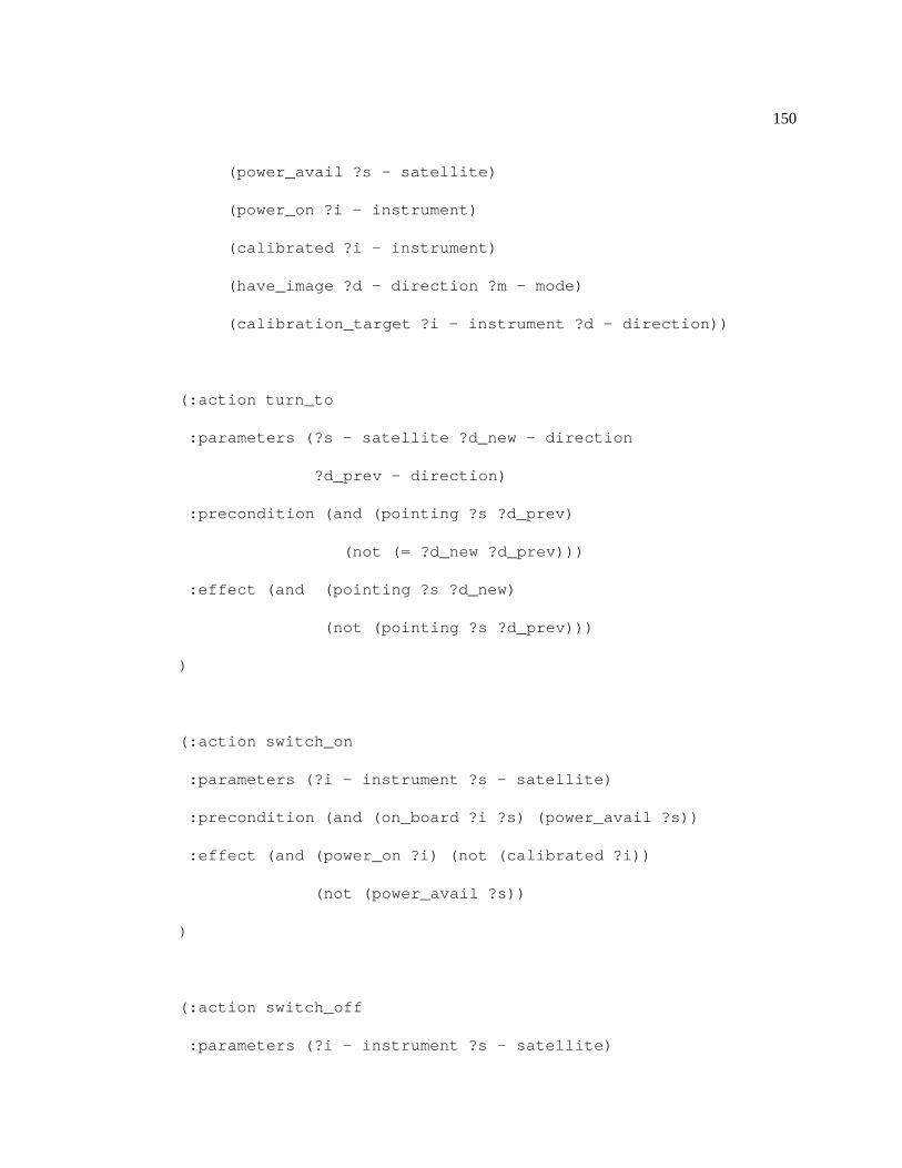
150
(power_avail ?s - satellite)
(power_on ?i - instrument)
(calibrated ?i - instrument)
(have_image ?d - direction ?m - mode)
(calibration_target ?i - instrument ?d - direction))
(:action turn_to
:parameters (?s - satellite ?d_new - direction
?d_prev - direction)
:precondition (and (pointing ?s ?d_prev)
(not (= ?d_new ?d_prev)))
:effect (and (pointing ?s ?d_new)
(not (pointing ?s ?d_prev)))
)
(:action switch_on
:parameters (?i - instrument ?s - satellite)
:precondition (and (on_board ?i ?s) (power_avail ?s))
:effect (and (power_on ?i) (not (calibrated ?i))
(not (power_avail ?s))
)
(:action switch_off
:parameters (?i - instrument ?s - satellite)
151
:precondition (and (on_board ?i ?s) (power_on ?i))
:effect (and (not (power_on ?i)) (power_avail ?s))
)
(:action calibrate
:parameters (?s - satellite ?i - instrument ?d - direction)
:precondition (and (on_board ?i ?s) (pointing ?s ?d)
(calibration_target ?i ?d) (power_on ?i))
:effect (calibrated ?i)
)
(:action take_image
:parameters (?s - satellite ?d - direction
?i - instrument ?m - mode)
:precondition (and (calibrated ?i) (on_board ?i ?s)
(supports ?i ?m) (power_on ?i)
(pointing ?s ?d) (power_on ?i))
:effect (have_image ?d ?m)
)
)
A.1.2. Problem Specification: Satellite.
(define (problem strips-sat-x-1)
(:domain satellite)
152
(:objects
satellite0 satellite1 - satellite
instrument0 instrument1 instrument2 - instrument
infrared0 infrared1 thermograph2 - mode
GroundStation1 Star0 Star2 Planet3 Star4
Planet5 Star6 Star7 Phenomenon8 Phenomenon9 - direction
)
(:init
(supports instrument0 thermograph2)
(supports instrument0 infrared0)
(calibration_target instrument0 Star0)
(on_board instrument0 satellite0)
(power_avail satellite0)
(pointing satellite0 Star6)
(supports instrument1 infrared0)
(supports instrument1 thermograph2)
(supports instrument1 infrared1)
(calibration_target instrument1 Star2)
(supports instrument2 thermograph2)
(supports instrument2 infrared1)
(calibration_target instrument2 Star2)
(on_board instrument1 satellite1)
(on_board instrument2 satellite1)
(power_avail satellite1)
153
(pointing satellite1 Star0)
)
(:goal (and
(pointing satellite1 Planet5)
(have_image Planet3 infrared1)
(have_image Star4 infrared1)
(have_image Planet5 thermograph2)
(have_image Star6 infrared1)
(have_image Star7 infrared0)
(have_image Phenomenon8 thermograph2)
(have_image Phenomenon9 infrared0))
)
)
A.2. Metric Temporal Planning with PDDL2.1 Planning Language
A.2.1. Domain Specification: Satellite.
(define (domain satellite)
(:requirements :strips :typing :fluents :durative-actions)
(:types satellite direction instrument mode)
(:predicates
(on_board ?i - instrument ?s - satellite)
(supports ?i - instrument ?m - mode)
(pointing ?s - satellite ?d - direction)
(power_avail ?s - satellite)
154
(power_on ?i - instrument)
(calibrated ?i - instrument)
(have_image ?d - direction ?m - mode)
(calibration_target ?i - instrument ?d - direction))
(:functions (slew_time ?a ?b - direction)
(calibration_time ?a - instrument ?d - direction)
(data_capacity ?s - satellite)
(data ?d - direction ?m - mode)
(data-stored)
)
(:durative-action turn_to
:parameters (?s - satellite ?d_new - direction
?d_prev - direction)
:duration (= ?duration (slew_time ?d_prev ?d_new))
:condition (and (at start (pointing ?s ?d_prev))
(over all (not (= ?d_new ?d_prev))))
:effect (and (at end (pointing ?s ?d_new))
(at start (not (pointing ?s ?d_prev))))
)
(:durative-action switch_on
:parameters (?i - instrument ?s - satellite)
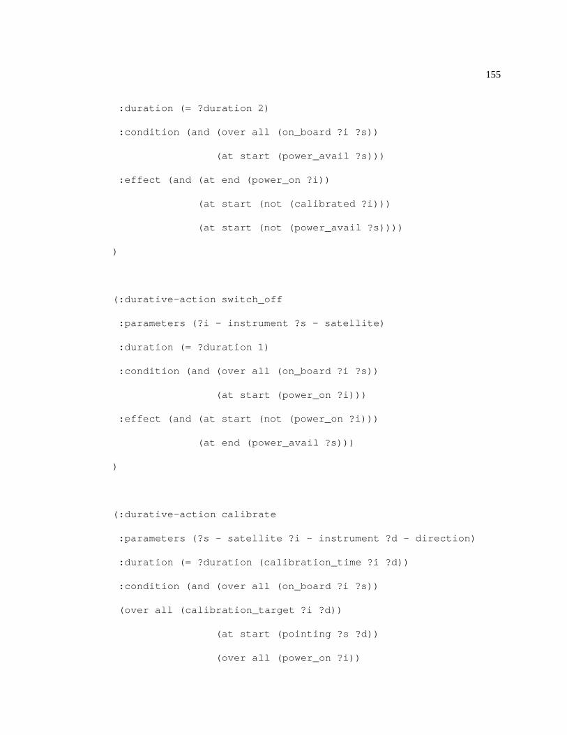
155
:duration (= ?duration 2)
:condition (and (over all (on_board ?i ?s))
(at start (power_avail ?s)))
:effect (and (at end (power_on ?i))
(at start (not (calibrated ?i)))
(at start (not (power_avail ?s))))
)
(:durative-action switch_off
:parameters (?i - instrument ?s - satellite)
:duration (= ?duration 1)
:condition (and (over all (on_board ?i ?s))
(at start (power_on ?i)))
:effect (and (at start (not (power_on ?i)))
(at end (power_avail ?s)))
)
(:durative-action calibrate
:parameters (?s - satellite ?i - instrument ?d - direction)
:duration (= ?duration (calibration_time ?i ?d))
:condition (and (over all (on_board ?i ?s))
(over all (calibration_target ?i ?d))
(at start (pointing ?s ?d))
(over all (power_on ?i))
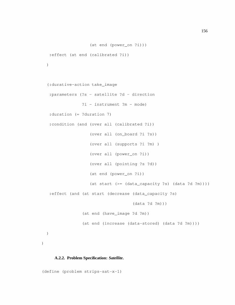
156
(at end (power_on ?i)))
:effect (at end (calibrated ?i))
)
(:durative-action take_image
:parameters (?s - satellite ?d - direction
?i - instrument ?m - mode)
:duration (= ?duration 7)
:condition (and (over all (calibrated ?i))
(over all (on_board ?i ?s))
(over all (supports ?i ?m) )
(over all (power_on ?i))
(over all (pointing ?s ?d))
(at end (power_on ?i))
(at start (>= (data_capacity ?s) (data ?d ?m))))
:effect (and (at start (decrease (data_capacity ?s)
(data ?d ?m)))
(at end (have_image ?d ?m))
(at end (increase (data-stored) (data ?d ?m))))
)
)
A.2.2. Problem Specification: Satellite.
(define (problem strips-sat-x-1)
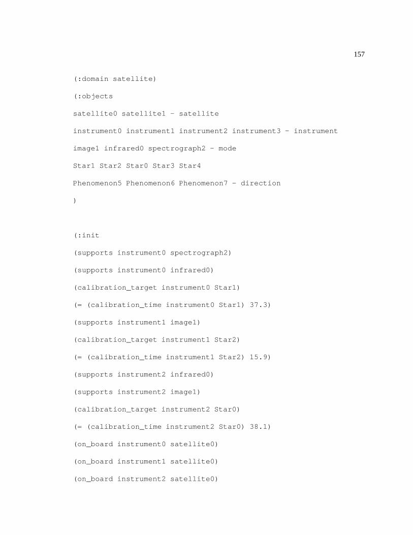
157
(:domain satellite)
(:objects
satellite0 satellite1 - satellite
instrument0 instrument1 instrument2 instrument3 - instrument
image1 infrared0 spectrograph2 - mode
Star1 Star2 Star0 Star3 Star4
Phenomenon5 Phenomenon6 Phenomenon7 - direction
)
(:init
(supports instrument0 spectrograph2)
(supports instrument0 infrared0)
(calibration_target instrument0 Star1)
(= (calibration_time instrument0 Star1) 37.3)
(supports instrument1 image1)
(calibration_target instrument1 Star2)
(= (calibration_time instrument1 Star2) 15.9)
(supports instrument2 infrared0)
(supports instrument2 image1)
(calibration_target instrument2 Star0)
(= (calibration_time instrument2 Star0) 38.1)
(on_board instrument0 satellite0)
(on_board instrument1 satellite0)
(on_board instrument2 satellite0)
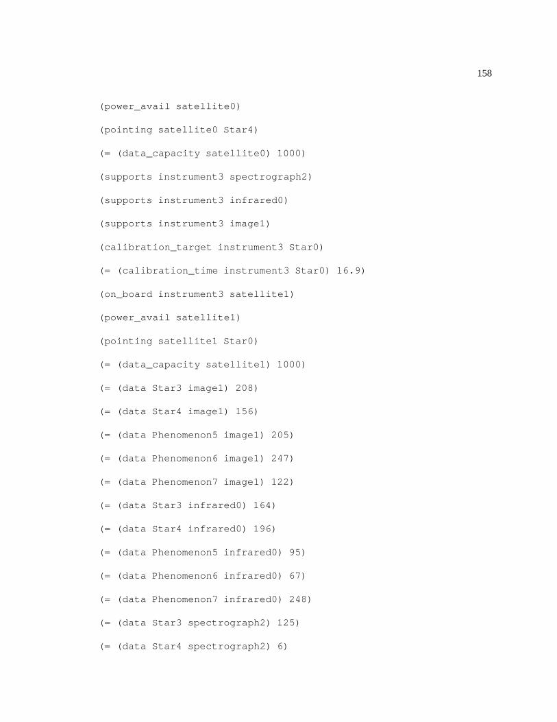
158
(power_avail satellite0)
(pointing satellite0 Star4)
(= (data_capacity satellite0) 1000)
(supports instrument3 spectrograph2)
(supports instrument3 infrared0)
(supports instrument3 image1)
(calibration_target instrument3 Star0)
(= (calibration_time instrument3 Star0) 16.9)
(on_board instrument3 satellite1)
(power_avail satellite1)
(pointing satellite1 Star0)
(= (data_capacity satellite1) 1000)
(= (data Star3 image1) 208)
(= (data Star4 image1) 156)
(= (data Phenomenon5 image1) 205)
(= (data Phenomenon6 image1) 247)
(= (data Phenomenon7 image1) 122)
(= (data Star3 infrared0) 164)
(= (data Star4 infrared0) 196)
(= (data Phenomenon5 infrared0) 95)
(= (data Phenomenon6 infrared0) 67)
(= (data Phenomenon7 infrared0) 248)
(= (data Star3 spectrograph2) 125)
(= (data Star4 spectrograph2) 6)
159
(= (data Phenomenon5 spectrograph2) 44)
(= (data Phenomenon6 spectrograph2) 222)
(= (data Phenomenon7 spectrograph2) 78)
(= (slew_time Star1 Star0) 34.35)
(= (slew_time Star0 Star1) 34.35)
(= (slew_time Star2 Star0) 8.768)
(= (slew_time Star0 Star2) 8.768)
(= (slew_time Star2 Star1) 18.57)
(= (slew_time Star1 Star2) 18.57)
(= (slew_time Star3 Star0) 25.66)
(= (slew_time Star0 Star3) 25.66)
(= (slew_time Star3 Star1) 25.96)
(= (slew_time Star1 Star3) 25.96)
(= (slew_time Star3 Star2) 17.99)
(= (slew_time Star2 Star3) 17.99)
(= (slew_time Star4 Star0) 71.99)
(= (slew_time Star0 Star4) 71.99)
(= (slew_time Star4 Star1) 1.526)
(= (slew_time Star1 Star4) 1.526)
(= (slew_time Star4 Star2) 35.34)
(= (slew_time Star2 Star4) 35.34)
(= (slew_time Star4 Star3) 49.61)
(= (slew_time Star3 Star4) 49.61)
(= (slew_time Phenomenon5 Star0) 67.92)
160
(= (slew_time Star0 Phenomenon5) 67.92)
(= (slew_time Phenomenon5 Star1) 4.095)
(= (slew_time Star1 Phenomenon5) 4.095)
(= (slew_time Phenomenon5 Star2) 30.24)
(= (slew_time Star2 Phenomenon5) 30.24)
(= (slew_time Phenomenon5 Star3) 7.589)
(= (slew_time Star3 Phenomenon5) 7.589)
(= (slew_time Phenomenon5 Star4) 0.5297)
(= (slew_time Star4 Phenomenon5) 0.5297)
(= (slew_time Phenomenon6 Star0) 77.1)
(= (slew_time Star0 Phenomenon6) 77.1)
(= (slew_time Phenomenon6 Star1) 47.3)
(= (slew_time Star1 Phenomenon6) 47.3)
(= (slew_time Phenomenon6 Star2) 64.11)
(= (slew_time Star2 Phenomenon6) 64.11)
(= (slew_time Phenomenon6 Star3) 51.56)
(= (slew_time Star3 Phenomenon6) 51.56)
(= (slew_time Phenomenon6 Star4) 56.36)
(= (slew_time Star4 Phenomenon6) 56.36)
(= (slew_time Phenomenon6 Phenomenon5) 67.57)
(= (slew_time Phenomenon5 Phenomenon6) 67.57)
(= (slew_time Phenomenon7 Star0) 9.943)
(= (slew_time Star0 Phenomenon7) 9.943)
(= (slew_time Phenomenon7 Star1) 13.3)
161
(= (slew_time Star1 Phenomenon7) 13.3)
(= (slew_time Phenomenon7 Star2) 60.53)
(= (slew_time Star2 Phenomenon7) 60.53)
(= (slew_time Phenomenon7 Star3) 53.93)
(= (slew_time Star3 Phenomenon7) 53.93)
(= (slew_time Phenomenon7 Star4) 67.87)
(= (slew_time Star4 Phenomenon7) 67.87)
(= (slew_time Phenomenon7 Phenomenon5) 43.97)
(= (slew_time Phenomenon5 Phenomenon7) 43.97)
(= (slew_time Phenomenon7 Phenomenon6) 32.34)
(= (slew_time Phenomenon6 Phenomenon7) 32.34)
(= (data-stored) 0)
)
(:goal (and
(pointing satellite0 Phenomenon5)
(have_image Star3 infrared0)
(have_image Star4 spectrograph2)
(have_image Phenomenon5 spectrograph2)
(have_image Phenomenon7 spectrograph2)
))
(:metric minimize (total-time)))
162
A.3. Extending PDDL2.1 for PSP Net Benefit
A.3.1. Domain Specification: ZenoTravel.
(define (domain zeno-travel)
(:requirements :durative-actions :typing :fluents)
(:types aircraft person city - object)
(:predicates (at ?x - (either person aircraft) ?c - city)
(in ?p - person ?a - aircraft))
(:functions (fuel ?a - aircraft)
(distance ?c1 - city ?c2 - city)
(slow-speed ?a - aircraft)
(fast-speed ?a - aircraft)
(slow-burn ?a - aircraft)
(fast-burn ?a - aircraft)
(capacity ?a - aircraft)
(refuel-rate ?a - aircraft)
(total-fuel-used)
(boarding-time ?c - city)
(debarking-time ?c - city)
(labor-cost ?c - city)
(fuel-cost ?c - city)
(maintainance-cost ?a - aircraft)
(airport-aircraft-fee ?a - aircraft ?c - city)
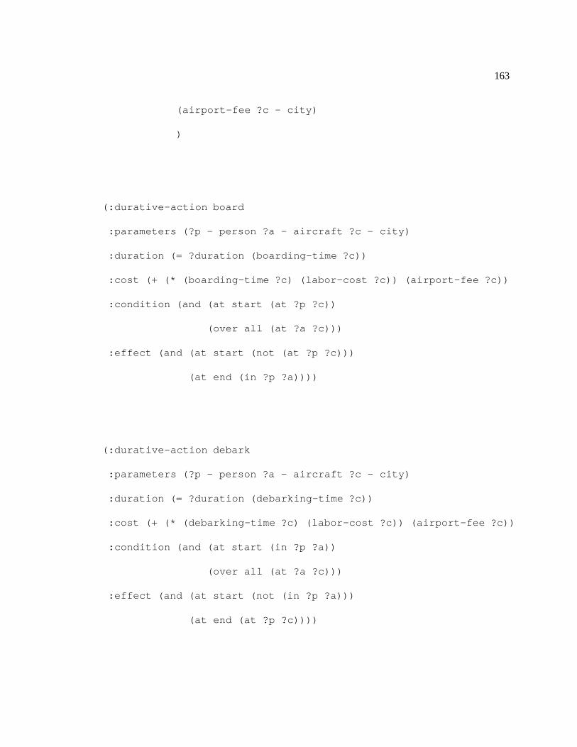
163
(airport-fee ?c - city)
)
(:durative-action board
:parameters (?p - person ?a - aircraft ?c - city)
:duration (= ?duration (boarding-time ?c))
:cost (+ (* (boarding-time ?c) (labor-cost ?c)) (airport-fee ?c))
:condition (and (at start (at ?p ?c))
(over all (at ?a ?c)))
:effect (and (at start (not (at ?p ?c)))
(at end (in ?p ?a))))
(:durative-action debark
:parameters (?p - person ?a - aircraft ?c - city)
:duration (= ?duration (debarking-time ?c))
:cost (+ (* (debarking-time ?c) (labor-cost ?c)) (airport-fee ?c))
:condition (and (at start (in ?p ?a))
(over all (at ?a ?c)))
:effect (and (at start (not (in ?p ?a)))
(at end (at ?p ?c))))
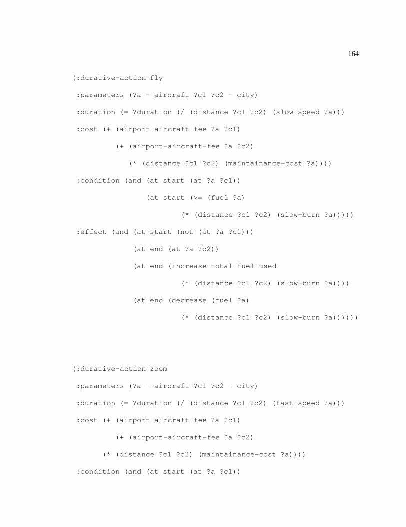
164
(:durative-action fly
:parameters (?a - aircraft ?c1 ?c2 - city)
:duration (= ?duration (/ (distance ?c1 ?c2) (slow-speed ?a)))
:cost (+ (airport-aircraft-fee ?a ?c1)
(+ (airport-aircraft-fee ?a ?c2)
(* (distance ?c1 ?c2) (maintainance-cost ?a))))
:condition (and (at start (at ?a ?c1))
(at start (>= (fuel ?a)
(* (distance ?c1 ?c2) (slow-burn ?a)))))
:effect (and (at start (not (at ?a ?c1)))
(at end (at ?a ?c2))
(at end (increase total-fuel-used
(* (distance ?c1 ?c2) (slow-burn ?a))))
(at end (decrease (fuel ?a)
(* (distance ?c1 ?c2) (slow-burn ?a))))))
(:durative-action zoom
:parameters (?a - aircraft ?c1 ?c2 - city)
:duration (= ?duration (/ (distance ?c1 ?c2) (fast-speed ?a)))
:cost (+ (airport-aircraft-fee ?a ?c1)
(+ (airport-aircraft-fee ?a ?c2)
(* (distance ?c1 ?c2) (maintainance-cost ?a))))
:condition (and (at start (at ?a ?c1))
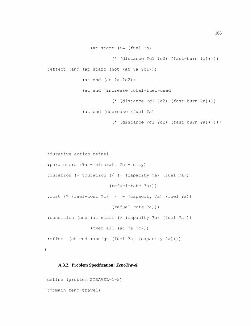
165
(at start (>= (fuel ?a)
(* (distance ?c1 ?c2) (fast-burn ?a)))))
:effect (and (at start (not (at ?a ?c1)))
(at end (at ?a ?c2))
(at end (increase total-fuel-used
(* (distance ?c1 ?c2) (fast-burn ?a))))
(at end (decrease (fuel ?a)
(* (distance ?c1 ?c2) (fast-burn ?a))))))
(:durative-action refuel
:parameters (?a - aircraft ?c - city)
:duration (= ?duration (/ (- (capacity ?a) (fuel ?a))
(refuel-rate ?a)))
:cost (* (fuel-cost ?c) (/ (- (capacity ?a) (fuel ?a))
(refuel-rate ?a)))
:condition (and (at start (> (capacity ?a) (fuel ?a)))
(over all (at ?a ?c)))
:effect (at end (assign (fuel ?a) (capacity ?a))))
)
A.3.2. Problem Specification: ZenoTravel.
(define (problem ZTRAVEL-1-2)
(:domain zeno-travel)

166
(:objects
plane1 - aircraft
person1 person2 - person
city0 city1 city2 - city
)
(:init
(at plane1 city0)
(at person1 city0)
(at person2 city2)
(= (slow-speed plane1) 198)
(= (fast-speed plane1) 449)
(= (capacity plane1) 10232)
(= (fuel plane1) 3956)
(= (slow-burn plane1) 4)
(= (fast-burn plane1) 15)
(= (refuel-rate plane1) 2904)
(= (distance city0 city0) 0)
(= (distance city0 city1) 678)
(= (distance city0 city2) 775)
(= (distance city1 city0) 678)
(= (distance city1 city1) 0)
(= (distance city1 city2) 810)
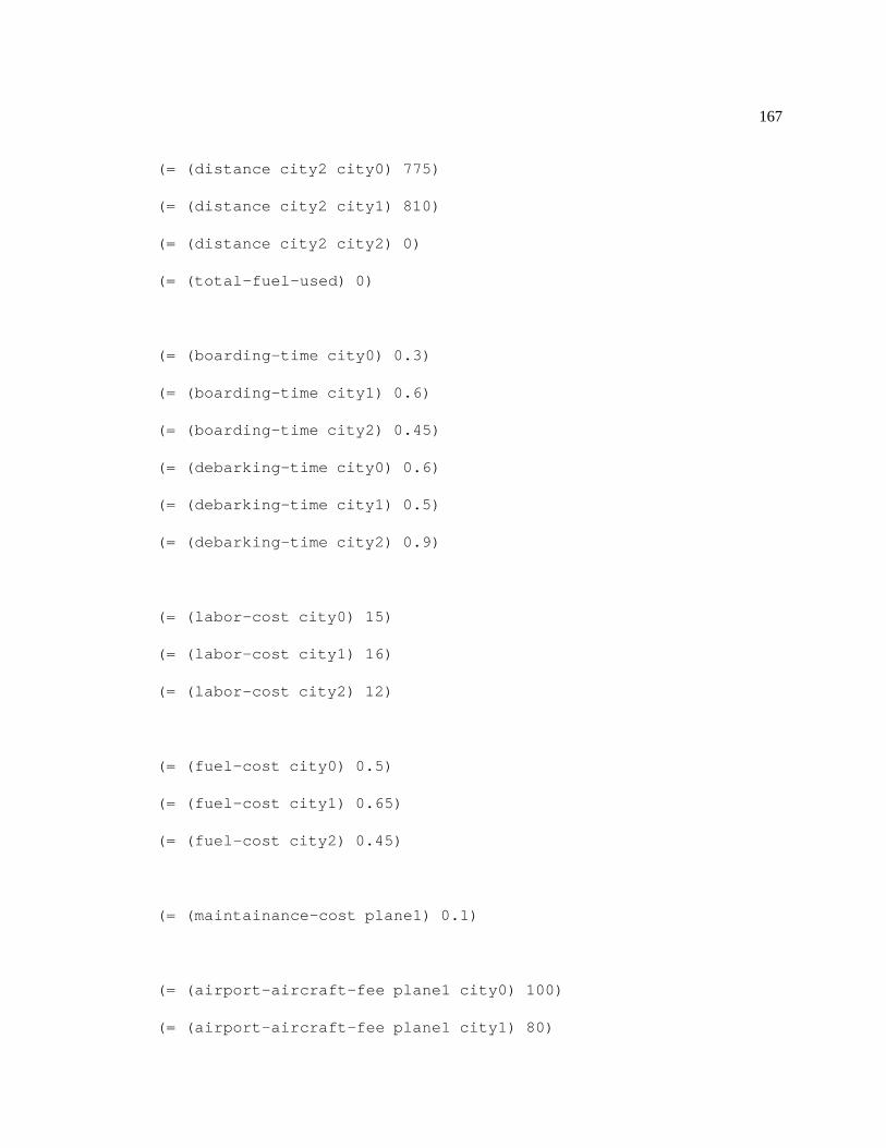
167
(= (distance city2 city0) 775)
(= (distance city2 city1) 810)
(= (distance city2 city2) 0)
(= (total-fuel-used) 0)
(= (boarding-time city0) 0.3)
(= (boarding-time city1) 0.6)
(= (boarding-time city2) 0.45)
(= (debarking-time city0) 0.6)
(= (debarking-time city1) 0.5)
(= (debarking-time city2) 0.9)
(= (labor-cost city0) 15)
(= (labor-cost city1) 16)
(= (labor-cost city2) 12)
(= (fuel-cost city0) 0.5)
(= (fuel-cost city1) 0.65)
(= (fuel-cost city2) 0.45)
(= (maintainance-cost plane1) 0.1)
(= (airport-aircraft-fee plane1 city0) 100)
(= (airport-aircraft-fee plane1 city1) 80)
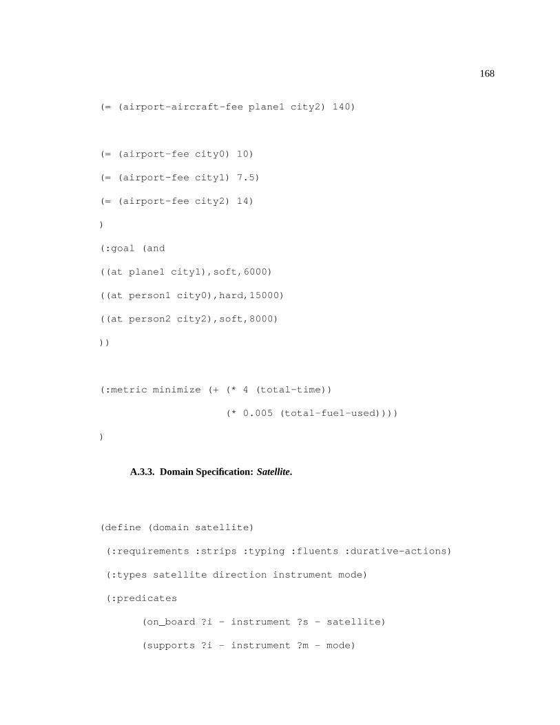
168
(= (airport-aircraft-fee plane1 city2) 140)
(= (airport-fee city0) 10)
(= (airport-fee city1) 7.5)
(= (airport-fee city2) 14)
)
(:goal (and
((at plane1 city1),soft,6000)
((at person1 city0),hard,15000)
((at person2 city2),soft,8000)
))
(:metric minimize (+ (* 4 (total-time))
(* 0.005 (total-fuel-used))))
)
A.3.3. Domain Specification: Satellite.
(define (domain satellite)
(:requirements :strips :typing :fluents :durative-actions)
(:types satellite direction instrument mode)
(:predicates
(on_board ?i - instrument ?s - satellite)
(supports ?i - instrument ?m - mode)
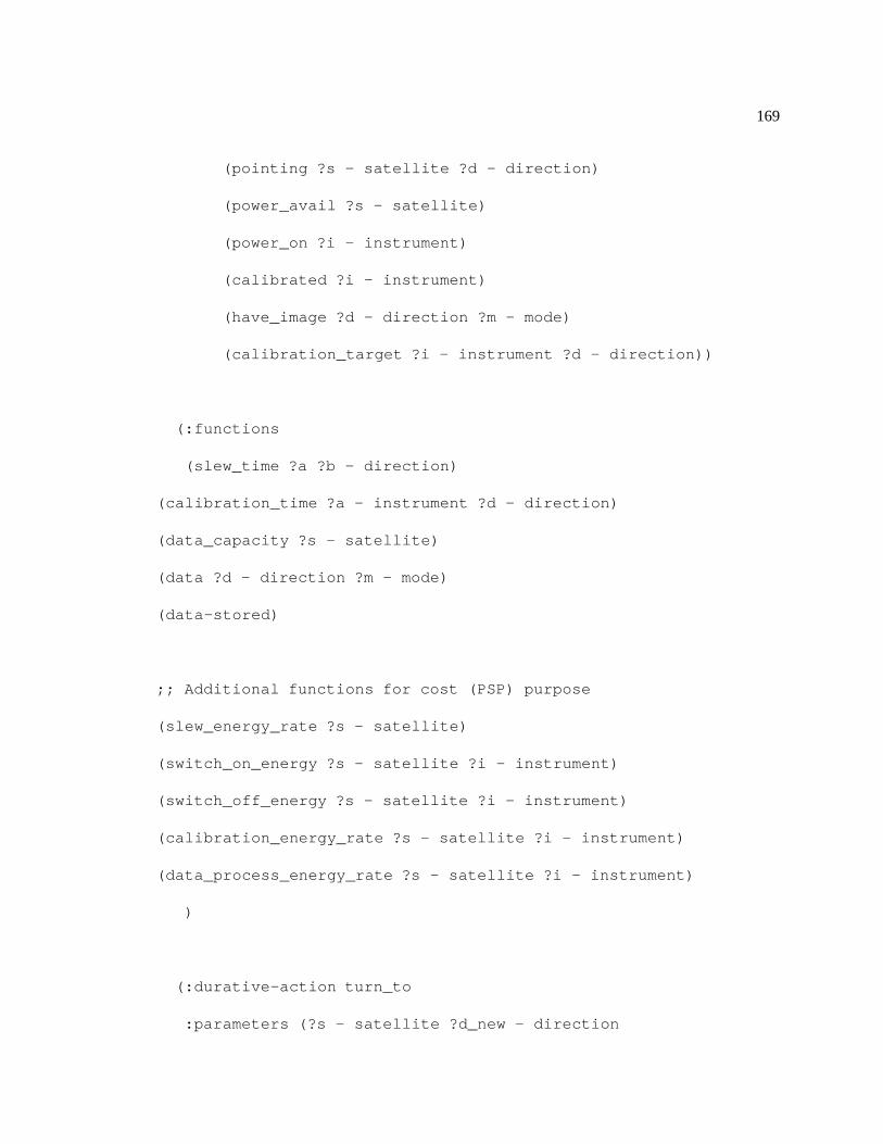
169
(pointing ?s - satellite ?d - direction)
(power_avail ?s - satellite)
(power_on ?i - instrument)
(calibrated ?i - instrument)
(have_image ?d - direction ?m - mode)
(calibration_target ?i - instrument ?d - direction))
(:functions
(slew_time ?a ?b - direction)
(calibration_time ?a - instrument ?d - direction)
(data_capacity ?s - satellite)
(data ?d - direction ?m - mode)
(data-stored)
;; Additional functions for cost (PSP) purpose
(slew_energy_rate ?s - satellite)
(switch_on_energy ?s - satellite ?i - instrument)
(switch_off_energy ?s - satellite ?i - instrument)
(calibration_energy_rate ?s - satellite ?i - instrument)
(data_process_energy_rate ?s - satellite ?i - instrument)
)
(:durative-action turn_to
:parameters (?s - satellite ?d_new - direction
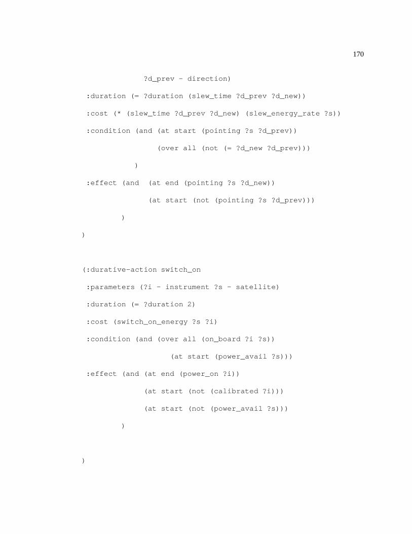
170
?d_prev - direction)
:duration (= ?duration (slew_time ?d_prev ?d_new))
:cost (* (slew_time ?d_prev ?d_new) (slew_energy_rate ?s))
:condition (and (at start (pointing ?s ?d_prev))
(over all (not (= ?d_new ?d_prev)))
)
:effect (and (at end (pointing ?s ?d_new))
(at start (not (pointing ?s ?d_prev)))
)
)
(:durative-action switch_on
:parameters (?i - instrument ?s - satellite)
:duration (= ?duration 2)
:cost (switch_on_energy ?s ?i)
:condition (and (over all (on_board ?i ?s))
(at start (power_avail ?s)))
:effect (and (at end (power_on ?i))
(at start (not (calibrated ?i)))
(at start (not (power_avail ?s)))
)
)
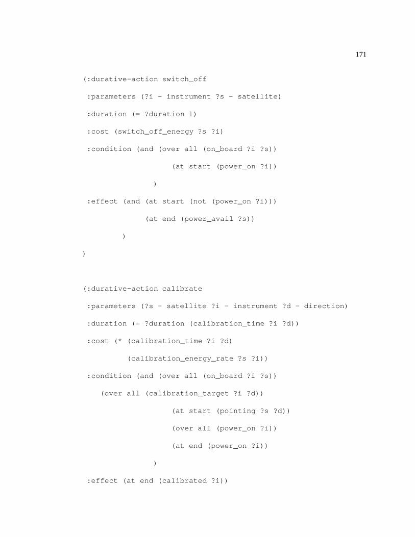
171
(:durative-action switch_off
:parameters (?i - instrument ?s - satellite)
:duration (= ?duration 1)
:cost (switch_off_energy ?s ?i)
:condition (and (over all (on_board ?i ?s))
(at start (power_on ?i))
)
:effect (and (at start (not (power_on ?i)))
(at end (power_avail ?s))
)
)
(:durative-action calibrate
:parameters (?s - satellite ?i - instrument ?d - direction)
:duration (= ?duration (calibration_time ?i ?d))
:cost (* (calibration_time ?i ?d)
(calibration_energy_rate ?s ?i))
:condition (and (over all (on_board ?i ?s))
(over all (calibration_target ?i ?d))
(at start (pointing ?s ?d))
(over all (power_on ?i))
(at end (power_on ?i))
)
:effect (at end (calibrated ?i))
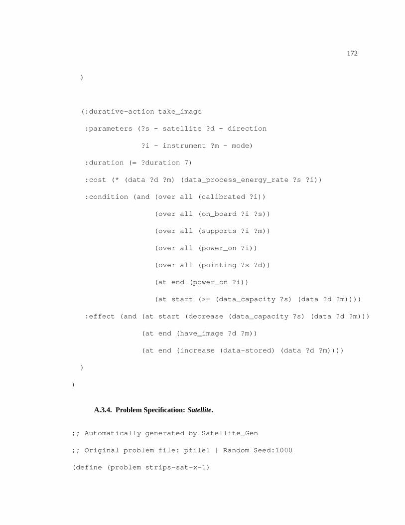
172
)
(:durative-action take_image
:parameters (?s - satellite ?d - direction
?i - instrument ?m - mode)
:duration (= ?duration 7)
:cost (* (data ?d ?m) (data_process_energy_rate ?s ?i))
:condition (and (over all (calibrated ?i))
(over all (on_board ?i ?s))
(over all (supports ?i ?m))
(over all (power_on ?i))
(over all (pointing ?s ?d))
(at end (power_on ?i))
(at start (>= (data_capacity ?s) (data ?d ?m))))
:effect (and (at start (decrease (data_capacity ?s) (data ?d ?m)))
(at end (have_image ?d ?m))
(at end (increase (data-stored) (data ?d ?m))))
)
)
A.3.4. Problem Specification: Satellite.
;; Automatically generated by Satellite_Gen
;; Original problem file: pfile1 | Random Seed:1000
(define (problem strips-sat-x-1)
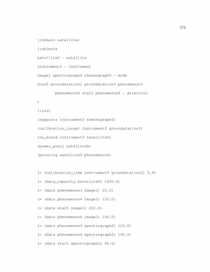
173
(:domain satellite)
(:objects
satellite0 - satellite
instrument0 - instrument
image1 spectrograph2 thermograph0 - mode
star0 groundstation1 groundstation2 phenomenon3
phenomenon4 star5 phenomenon6 - direction
)
(:init
(supports instrument0 thermograph0)
(calibration_target instrument0 groundstation2)
(on_board instrument0 satellite0)
(power_avail satellite0)
(pointing satellite0 phenomenon6)
(= (calibration_time instrument0 groundstation2) 5.9)
(= (data_capacity satellite0) 1000.0)
(= (data phenomenon3 image1) 22.0)
(= (data phenomenon4 image1) 120.0)
(= (data star5 image1) 203.0)
(= (data phenomenon6 image1) 144.0)
(= (data phenomenon3 spectrograph2) 125.0)
(= (data phenomenon4 spectrograph2) 196.0)
(= (data star5 spectrograph2) 68.0)
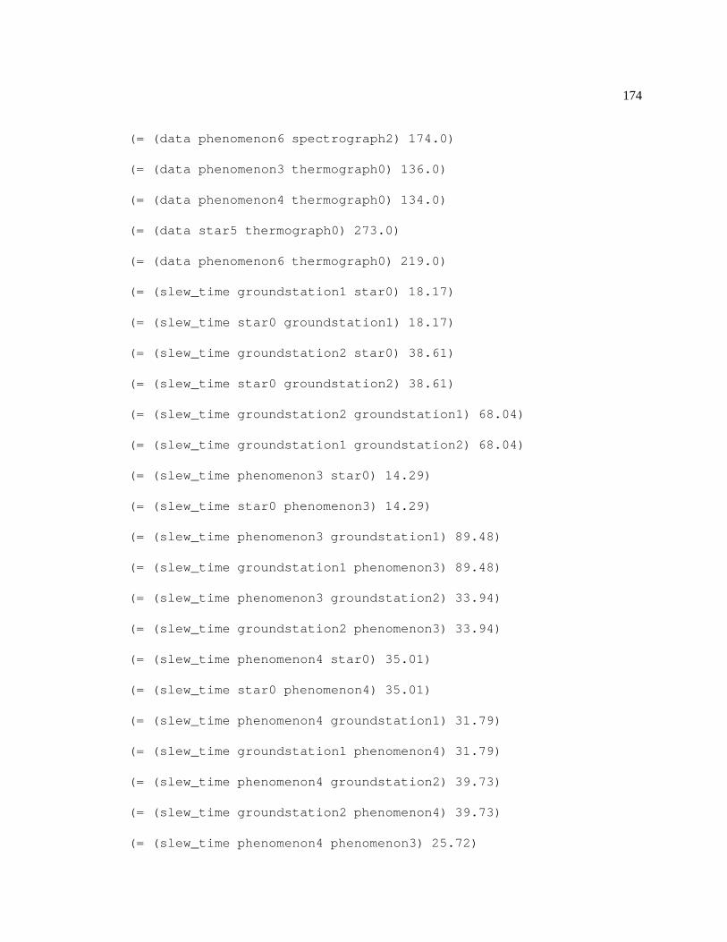
174
(= (data phenomenon6 spectrograph2) 174.0)
(= (data phenomenon3 thermograph0) 136.0)
(= (data phenomenon4 thermograph0) 134.0)
(= (data star5 thermograph0) 273.0)
(= (data phenomenon6 thermograph0) 219.0)
(= (slew_time groundstation1 star0) 18.17)
(= (slew_time star0 groundstation1) 18.17)
(= (slew_time groundstation2 star0) 38.61)
(= (slew_time star0 groundstation2) 38.61)
(= (slew_time groundstation2 groundstation1) 68.04)
(= (slew_time groundstation1 groundstation2) 68.04)
(= (slew_time phenomenon3 star0) 14.29)
(= (slew_time star0 phenomenon3) 14.29)
(= (slew_time phenomenon3 groundstation1) 89.48)
(= (slew_time groundstation1 phenomenon3) 89.48)
(= (slew_time phenomenon3 groundstation2) 33.94)
(= (slew_time groundstation2 phenomenon3) 33.94)
(= (slew_time phenomenon4 star0) 35.01)
(= (slew_time star0 phenomenon4) 35.01)
(= (slew_time phenomenon4 groundstation1) 31.79)
(= (slew_time groundstation1 phenomenon4) 31.79)
(= (slew_time phenomenon4 groundstation2) 39.73)
(= (slew_time groundstation2 phenomenon4) 39.73)
(= (slew_time phenomenon4 phenomenon3) 25.72)
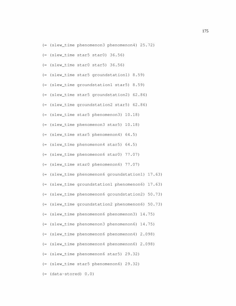
175
(= (slew_time phenomenon3 phenomenon4) 25.72)
(= (slew_time star5 star0) 36.56)
(= (slew_time star0 star5) 36.56)
(= (slew_time star5 groundstation1) 8.59)
(= (slew_time groundstation1 star5) 8.59)
(= (slew_time star5 groundstation2) 62.86)
(= (slew_time groundstation2 star5) 62.86)
(= (slew_time star5 phenomenon3) 10.18)
(= (slew_time phenomenon3 star5) 10.18)
(= (slew_time star5 phenomenon4) 64.5)
(= (slew_time phenomenon4 star5) 64.5)
(= (slew_time phenomenon6 star0) 77.07)
(= (slew_time star0 phenomenon6) 77.07)
(= (slew_time phenomenon6 groundstation1) 17.63)
(= (slew_time groundstation1 phenomenon6) 17.63)
(= (slew_time phenomenon6 groundstation2) 50.73)
(= (slew_time groundstation2 phenomenon6) 50.73)
(= (slew_time phenomenon6 phenomenon3) 14.75)
(= (slew_time phenomenon3 phenomenon6) 14.75)
(= (slew_time phenomenon6 phenomenon4) 2.098)
(= (slew_time phenomenon4 phenomenon6) 2.098)
(= (slew_time phenomenon6 star5) 29.32)
(= (slew_time star5 phenomenon6) 29.32)
(= (data-stored) 0.0)
176
;; (slew_energy_rate ?satellite) : 0.5 - 2 (random)
(= (slew_energy_rate satellite0) 1.57)
;; (switch_on_energy ?satellite ?instrument) : 10 - 20
(= (switch_on_energy satellite0 instrument0) 12.47)
;; (switch_off_energy ?satellite ?instrument) : 5 - 15
(= (switch_off_energy satellite0 instrument0) 10.75)
;; (calibration_energy_rate ?satellite ?instrument) : 20 - 40
(= (calibration_energy_rate satellite0 instrument0) 29.21)
;; (data_process_energy_rate ?satellite ?instrument) : 1 - 10
(= (data_process_energy_rate satellite0 instrument0) 9.52)
)
(:goal (and
;; Goals: (pointing ?sat ?dir) - soft
;; (have_image ?dir ?mode) 80% soft
;; Goal utility: random with bounds [2000 - 6000]
((have_image phenomenon4 thermograph0) hard 2157.62)
((have_image star5 thermograph0) soft 3945.64)
((have_image phenomenon6 thermograph0) soft 3782.95)
177
;; Additional goals. Utility: 1000-5000 (random)
((have_image star0 spectrograph2) soft 3403.26)
((have_image groundstation1 thermograph0) soft 3201.50)
((have_image groundstation2 image1) soft 3632.23)
((have_image phenomenon3 spectrograph2) soft 4897.99)
((pointing satellite0 star5) soft 3520.31)
)

APPENDIX B
CSOP and MILP Encoding
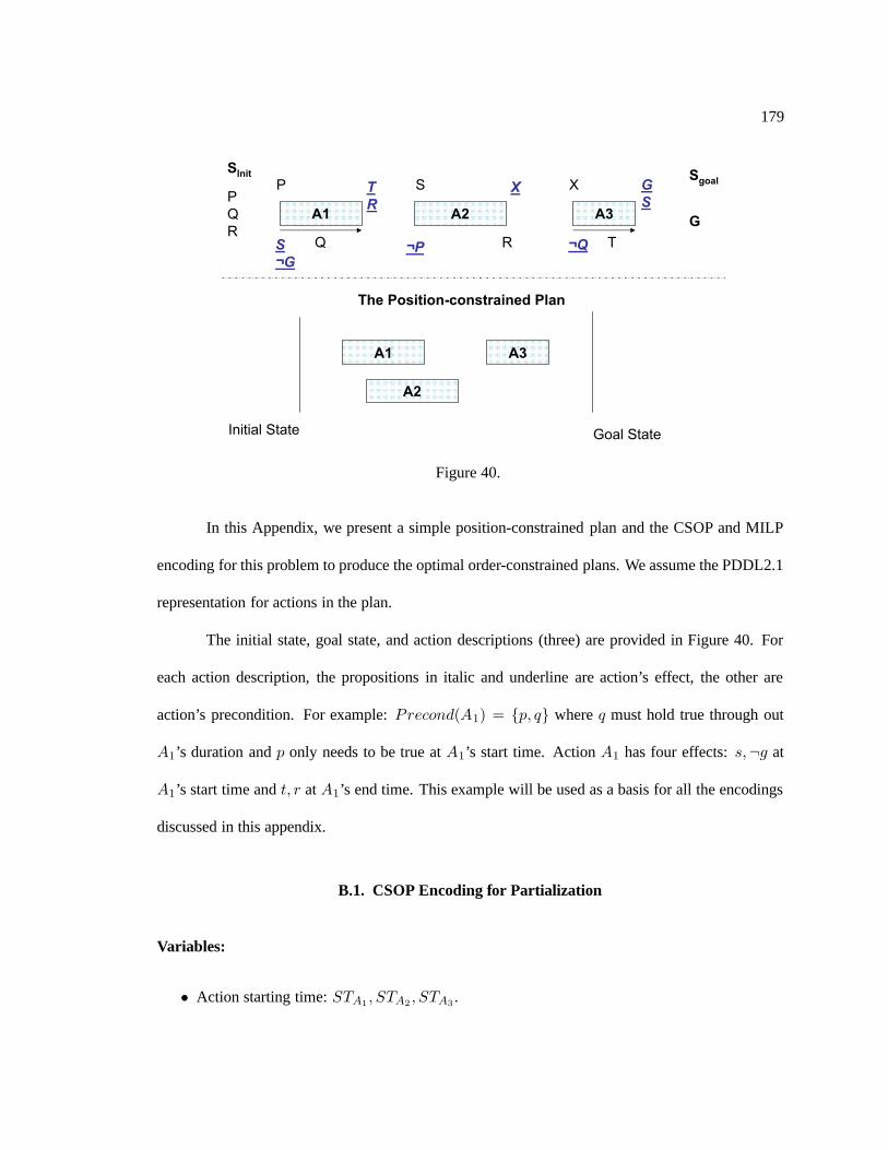
179
SInit
P
Q
R
A1
P
Q
T
R
S
¬G
A2
S
R
X
¬P
A3
X
T
G
S
¬Q
Sgoal
G
The Position-constrained Plan
A1
A2
A3
Initial State Goal State
Figure 40.
In this Appendix, we present a simple position-constrained plan and the CSOP and MILP
encoding for this problem to produce the optimal order-constrained plans. We assume the PDDL2.1
representation for actions in the plan.
The initial state, goal state, and action descriptions (three) are provided in Figure 40. For
each action description, the propositions in italic and underline are action’s effect, the other are
action’s precondition. For example: Precond(A1) = {p, q} where q must hold true through out
A1’s duration and p only needs to be true at A1’s start time. Action A1 has four effects: s,¬g at
A1’s start time and t, r at A1’s end time. This example will be used as a basis for all the encodings
discussed in this appendix.
B.1. CSOP Encoding for Partialization
Variables:
• Action starting time: STA1, STA2
, STA3.
180
• Causal effect for action’s conditions: SpA1
, SqA1
, SsA2
, SrA2
, SxA3
, StA3
. Variable domains:
Dom(SpA1
) = {Ainit}, Dom(SqA1
) = {Ainit}, Dom(SsA2
) = {A1, A3}, Dom(SrA2
) =
{Ainit, A1}, Dom(SxA3
) = {A2}, Dom(StA3
) = {A1}, Dom(SgAgoal
) = {A3}.
• Interference: IpA1A2
, IqA1A3
, IgA1A3
; interference variables are binary variables.
Constraints:
• Causal-link protection:
SpA1
= Ainit ⇒ IpA1A2
=≺
SqA1
= Ainit ⇒ IqA1A3
=≺
SgAgoal
= A3 ⇒ IgA1A3
=≺.
• Constraints between ordering variables and action starting times:
SsA2
= A1 ⇒ STA1< STA2
SrA2
= A1 ⇒ STA1+ DA1
< STA2+ DA1
SxA3
= A2 ⇒ STA2+ DA2
< STA3
SgAgoal
= A3 ⇒ STA3+ DA3
< STAgoal
IpA1A2
=≺⇔ STA1< STA2
IpA1A2
=�⇔ STA2< STA1
IqA1A3
=≺⇔ STA1+ DA1
< STA3
IqA1A3
=�⇔ STA1> STA3
...................
Objective functions: Minimal makespan: minimize STAgoal
B.2. MILP Encoding
Variables:
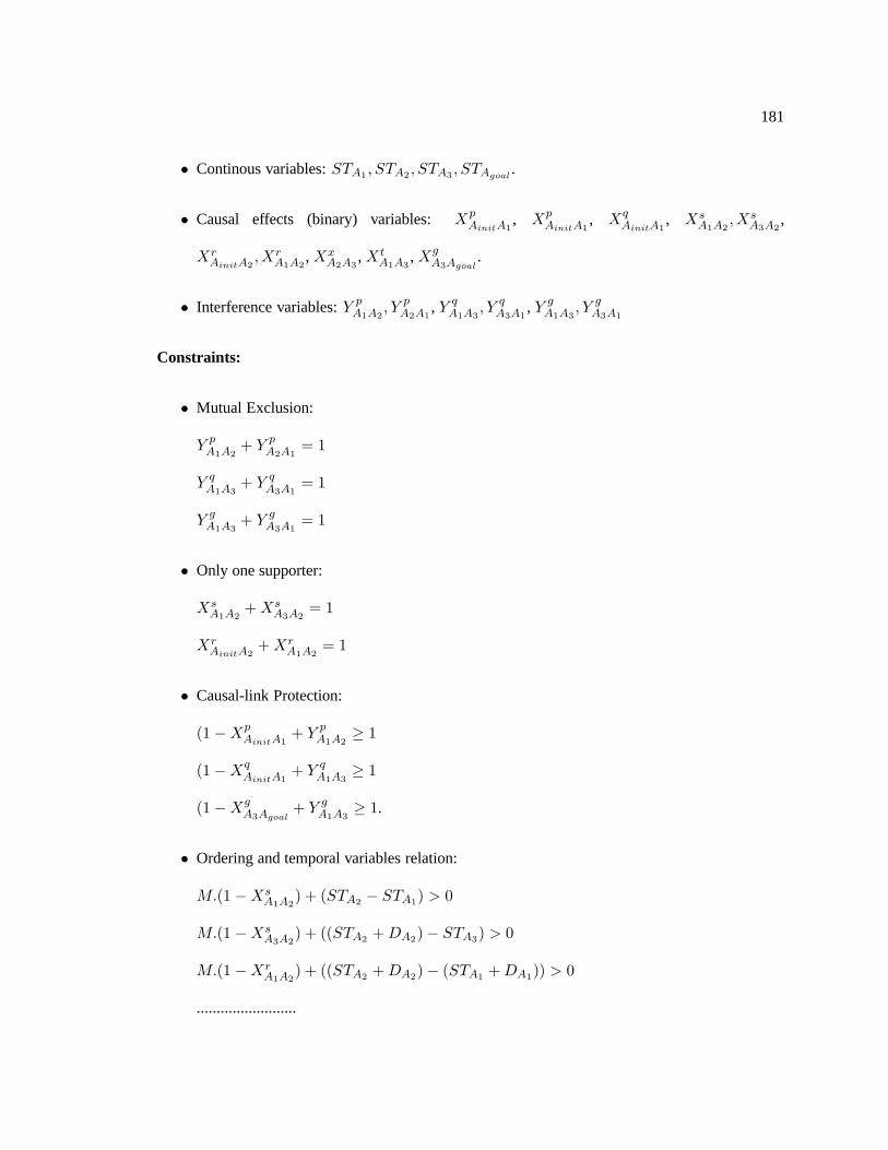
181
• Continous variables: STA1, STA2
, STA3, STAgoal
.
• Causal effects (binary) variables: XpAinitA1
, XpAinitA1
, XqAinitA1
, XsA1A2
, XsA3A2
,
XrAinitA2
, XrA1A2
, XxA2A3
, XtA1A3
, XgA3Agoal
.
• Interference variables: Y pA1A2
, Y pA2A1
, Y qA1A3
, Y qA3A1
, Y gA1A3
, Y gA3A1
Constraints:
• Mutual Exclusion:
Y pA1A2
+ Y pA2A1
= 1
Y qA1A3
+ Y qA3A1
= 1
Y gA1A3
+ Y gA3A1
= 1
• Only one supporter:
XsA1A2
+ XsA3A2
= 1
XrAinitA2
+ XrA1A2
= 1
• Causal-link Protection:
(1−XpAinitA1
+ Y pA1A2
≥ 1
(1−XqAinitA1
+ Y qA1A3
≥ 1
(1−XgA3Agoal
+ Y gA1A3
≥ 1.
• Ordering and temporal variables relation:
M.(1 −XsA1A2
) + (STA2− STA1
) > 0
M.(1 −XsA3A2
) + ((STA2+ DA2
)− STA3) > 0
M.(1 −XrA1A2
) + ((STA2+ DA2
)− (STA1+ DA1
)) > 0
.........................
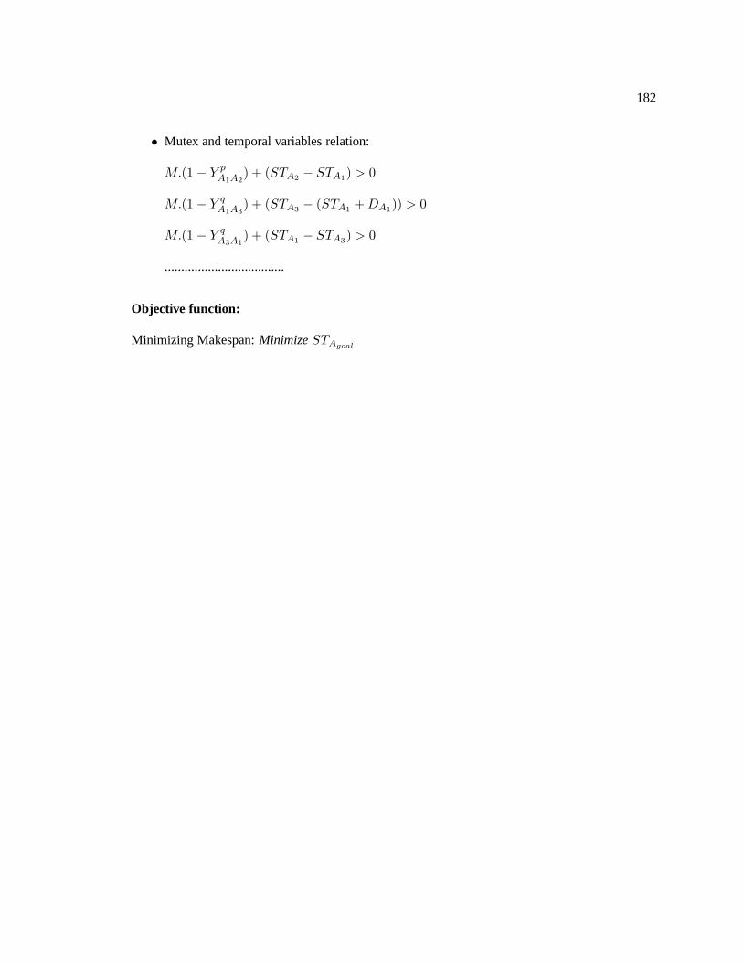
182
• Mutex and temporal variables relation:
M.(1 − Y pA1A2
) + (STA2− STA1
) > 0
M.(1 − Y qA1A3
) + (STA3− (STA1
+ DA1)) > 0
M.(1 − Y qA3A1
) + (STA1− STA3
) > 0
....................................
Objective function:
Minimizing Makespan: Minimize STAgoal