an analysis of cooperative coevolutionary ... - tesseract.org · an analysis of cooperative...

An Analysis of Cooperative Coevolutionary Algorithms

A dissertation submitted in partial fulfillment of the requirements for the degree of Doctor of Philosophy atGeorge Mason University

By

R. Paul WiegandBachelor of Science, Computer Science

Winthrop University, 1996Master of Science

University North Carolina Charlotte, 1999

Director: Kenneth A. De Jong,Professor, Department of Computer Science

Fall Semester 2003George Mason University

Fairfax, Virginia

ii

Copyright 2002 R. Paul WiegandAll Rights Reserved

iii

DEDICATION

To my wife Andrea, whose considerable counsel was only a small part of her contribution towards my successin completing this dissertation.

iv

ACKNOWLEDGEMENTS

I want to thank my committee members: Dr. Sauer, Dr. Hamburger, Dr. Luke, and Dr. De Jong. Inparticular, I would like thank Ken De Jong, whose advice and guiding hand has been a great source of help andunyielding service to me. Nearly all I know of Method comes from Ken and Descartes. If I master Methodhalf as well as either, I will consider myself very fortunate. I will also single out Sean Luke, whose constantcontrariness contributed to this work being about more thanmere nasal membrane (I hope).

The next big group of acknowledgments must go to my fellow labmates. Their considerable advice,support, and influence ranks among the most profound aspectsof my education. In particular, I thank LiviuPanait, Jeff Bassett, Jayshree Sarma, and Bill Liles. Additionally, I would like to thank Thomas Jansen, as wellas the entirety of Ingo Wegener’s chair at Dortmund University. Their helpful influence is clear in the first halfof my dissertation, but the extent of this influence cannot possibly be fully visible.

Because they deserve it and are not thanked nearly enough, I would also like to thank the staff of theDepartment of Computer Science at George Mason University.They are great group of people, who havealways gone out of their way to help make this process a littleeasier for me. Likewise, I thank the people atLibrary and Information Services. They do a huge and irreplaceable service for those of us in deep study, andprobably cannot be thanked enough.

On a personal level, I thank my wife for her support. She givesme strength and self confidence. Inexchange, I wash the clothes. I get the better end of that deal, I think. Finally, I want to be among the many whosay that life is an adventure of learning and for every question answered, there are a dozen more unansweredquestions that are uncovered. Far from being discouraging,this truism is one for which I was prepared...andone of the reasons I feel that life is worth living. This preparation, and this love of learning, I owe to my parents,who definitely cannot be thanked enough.

v

TABLE OF CONTENTS

PageAbstract . . . . . . . . . . . . . . . . . . . . . . . . . . . . . . . . . . . . . . . . . . .. . . . . . . . . . . . . . . . . . . . . . . . . . . . . . . . . . . . . . . . . . . . . . xi1 Introduction . . . . . . . . . . . . . . . . . . . . . . . . . . . . . . . . . . . . . .. . . . . . . . . . . . . . . . . . . . . . . . . . . . . . . . . . . . . . . . . . . . 1

1.1 Evolutionary Algorithms . . . . . . . . . . . . . . . . . . . . . . . . . .. . . . . . . . . . . . . . . . . . . . . . . . . . . . . . . . . . . . . . . . . 11.2 Coevolutionary Algorithms . . . . . . . . . . . . . . . . . . . . . . . .. . . . . . . . . . . . . . . . . . . . . . . . . . . . . . . . . . . . . . . . . 11.3 Understanding Cooperative Coevolution . . . . . . . . . . . . .. . . . . . . . . . . . . . . . . . . . . . . . . . . . . . . . . . . . . . . . 31.4 Organization . . . . . . . . . . . . . . . . . . . . . . . . . . . . . . . . . . . .. . . . . . . . . . . . . . . . . . . . . . . . . . . . . . . . . . . . . . . . . . 4

2 Background . . . . . . . . . . . . . . . . . . . . . . . . . . . . . . . . . . . . . . . .. . . . . . . . . . . . . . . . . . . . . . . . . . . . . . . . . . . . . . . . . . 72.1 Overview of Evolutionary Computation . . . . . . . . . . . . . . .. . . . . . . . . . . . . . . . . . . . . . . . . . . . . . . . . . . . . . 72.2 Overview of Coevolutionary Computation . . . . . . . . . . . . .. . . . . . . . . . . . . . . . . . . . . . . . . . . . . . . . . . . . . . 122.3 Background Work in Analysis of CoEC. . . . . . . . . . . . . . . . . .. . . . . . . . . . . . . . . . . . . . . . . . . . . . . . . . . . . . 17

3 Coevolutionary Architectures . . . . . . . . . . . . . . . . . . . . . . .. . . . . . . . . . . . . . . . . . . . . . . . . . . . . . . . . . . . . . . . . . . 213.1 Categorizing Coevolutionary Algorithms . . . . . . . . . . . .. . . . . . . . . . . . . . . . . . . . . . . . . . . . . . . . . . . . . . . . 213.2 A Cooperative Coevolutionary Algorithm . . . . . . . . . . . . .. . . . . . . . . . . . . . . . . . . . . . . . . . . . . . . . . . . . . . . 273.3 Optimizing with The CCEA . . . . . . . . . . . . . . . . . . . . . . . . . . .. . . . . . . . . . . . . . . . . . . . . . . . . . . . . . . . . . . . . 29

4 CCEAs as Static Optimizers . . . . . . . . . . . . . . . . . . . . . . . . . . .. . . . . . . . . . . . . . . . . . . . . . . . . . . . . . . . . . . . . . . . 334.1 Applying CCEAs. . . . . . . . . . . . . . . . . . . . . . . . . . . . . . . . . . .. . . . . . . . . . . . . . . . . . . . . . . . . . . . . . . . . . . . . . . 334.2 Partitioning and Focussing . . . . . . . . . . . . . . . . . . . . . . . .. . . . . . . . . . . . . . . . . . . . . . . . . . . . . . . . . . . . . . . . . 374.3 Collaboration . . . . . . . . . . . . . . . . . . . . . . . . . . . . . . . . . . .. . . . . . . . . . . . . . . . . . . . . . . . . . . . . . . . . . . . . . . . . . 484.4 Difficulties with CCEAs . . . . . . . . . . . . . . . . . . . . . . . . . . . .. . . . . . . . . . . . . . . . . . . . . . . . . . . . . . . . . . . . . . . 56

5 Optimization versus Balance . . . . . . . . . . . . . . . . . . . . . . . . .. . . . . . . . . . . . . . . . . . . . . . . . . . . . . . . . . . . . . . . . . . 635.1 CEAs are Not Static Optimizers of Ideal Partnership . . . .. . . . . . . . . . . . . . . . . . . . . . . . . . . . . . . . . . . . . . 635.2 Modeling CCEAs with EGT . . . . . . . . . . . . . . . . . . . . . . . . . . . .. . . . . . . . . . . . . . . . . . . . . . . . . . . . . . . . . . . . 665.3 Dynamical Systems Analysis . . . . . . . . . . . . . . . . . . . . . . . .. . . . . . . . . . . . . . . . . . . . . . . . . . . . . . . . . . . . . . . 735.4 Empirical Examples . . . . . . . . . . . . . . . . . . . . . . . . . . . . . . .. . . . . . . . . . . . . . . . . . . . . . . . . . . . . . . . . . . . . . . . 92

6 New Views of CCEAs . . . . . . . . . . . . . . . . . . . . . . . . . . . . . . . . . . .. . . . . . . . . . . . . . . . . . . . . . . . . . . . . . . . . . . . . . 976.1 Biasing Towards Static Optimization . . . . . . . . . . . . . . . .. . . . . . . . . . . . . . . . . . . . . . . . . . . . . . . . . . . . . . . . 976.2 Balancing Evolutionary Change. . . . . . . . . . . . . . . . . . . . .. . . . . . . . . . . . . . . . . . . . . . . . . . . . . . . . . . . . . . . . 1006.3 Optimizing for Robustness . . . . . . . . . . . . . . . . . . . . . . . . .. . . . . . . . . . . . . . . . . . . . . . . . . . . . . . . . . . . . . . . . 1026.4 Conclusions . . . . . . . . . . . . . . . . . . . . . . . . . . . . . . . . . . . . .. . . . . . . . . . . . . . . . . . . . . . . . . . . . . . . . . . . . . . . . . 1046.5 Future Research . . . . . . . . . . . . . . . . . . . . . . . . . . . . . . . . . .. . . . . . . . . . . . . . . . . . . . . . . . . . . . . . . . . . . . . . . . . 106

Bibliography . . . . . . . . . . . . . . . . . . . . . . . . . . . . . . . . . . . . . . .. . . . . . . . . . . . . . . . . . . . . . . . . . . . . . . . . . . . . . . . . . . . . 107

vii

LIST OF FIGURES

Figure Page

3.1 Hierarchical categorization of CEA properties. . . . . . .. . . . . . . . . . . . . . . . . . . . 233.2 Illustration of CCEA . . . . . . . . . . . . . . . . . . . . . . . . . . . . . .. . . . . . . . . 303.3 Illustration of a real-valued decomposition . . . . . . . . .. . . . . . . . . . . . . . . . . . . 313.4 Illustration of a binary decomposition . . . . . . . . . . . . . .. . . . . . . . . . . . . . . . 31

4.1 Illustration of partitioning . . . . . . . . . . . . . . . . . . . . . .. . . . . . . . . . . . . . . 354.2 Illustration of components versus pieces . . . . . . . . . . . .. . . . . . . . . . . . . . . . . 374.3 Results for CC (1+1) EA and (1+1) EA on CLOB2,4. . . . . . . . . . . . . . . . . . . . . . . 444.4 Results for CC (1+1) EA and (1+1) EA on LEADINGONES. . . . . . . . . . . . . . . . . . . 444.5 Results for SS-CCEA and SS-EA on CLOB2,4. . . . . . . . . . . . . . . . . . . . . . . . . . 454.6 Results for SS-CCEA and SS-EA on LEADINGONES. . . . . . . . . . . . . . . . . . . . . . . 454.7 Decompositional bias results for SS-CCEA ons·LEADINGONES−ONEMAX . . . . . . . . . 534.8 Collaboration selection results for SS-CCEA CLOB2,2 with maskMs . . . . . . . . . . . . . 574.9 Collaboration selection results for SS-CCEA CLOB2,2 with maskMs . . . . . . . . . . . . . 58

5.1 Payoff matrix examples . . . . . . . . . . . . . . . . . . . . . . . . . . . .. . . . . . . . . . 675.2 Example demonstrating meaning of termcorresponds. . . . . . . . . . . . . . . . . . . . . . 715.3 Illustration SIMPLEQUADRATIC function . . . . . . . . . . . . . . . . . . . . . . . . . . . . 735.4 Illustration MAX OFTWOQUADRATICS function withs1 = 2 . . . . . . . . . . . . . . . . . . 745.5 Illustration MAX OFTWOQUADRATICS function withs1 = 64 . . . . . . . . . . . . . . . . . 745.6 2D Takeover plot for SIMPLEQUADRATIC . . . . . . . . . . . . . . . . . . . . . . . . . . . . 795.7 Ratio of globally converged trajectories in MAX OFTWOQUADRATICS. . . . . . . . . . . . . 805.8 Trajectories on MAX OFTWOQUADRATICS with s1 ∈ 2,4,8,16,32,64 . . . . . . . . . . . . 825.9 2D takeover plots for uniform crossover . . . . . . . . . . . . . .. . . . . . . . . . . . . . . 875.10 2D takeover plots for uniform crossover with symmetricIC . . . . . . . . . . . . . . . . . . . 885.11 2D Takeover plots for bit-flip mutation. . . . . . . . . . . . . .. . . . . . . . . . . . . . . . 895.12 2D Takeover plots for mutation & crossover. . . . . . . . . . .. . . . . . . . . . . . . . . . . 905.13 CCEA and EA empirical results on MAX OFTWOQUADRATICS . . . . . . . . . . . . . . . . 945.14 CCEA and EA empirical results on ASYMMTWOQUAD without crossover . . . . . . . . . . . 955.15 CCEA fitness standard deviations on ASYMMTWOQUAD . . . . . . . . . . . . . . . . . . . . 96

6.1 Sensitivity of bias . . . . . . . . . . . . . . . . . . . . . . . . . . . . . . .. . . . . . . . . . 996.2 Spatial CCEA . . . . . . . . . . . . . . . . . . . . . . . . . . . . . . . . . . . . .. . . . . . 1006.3 Spatial CCEA empirical results on ASYMMTWOQUAD with crossover . . . . . . . . . . . . . 1026.4 Spatial CCEA fitness standard deviations on ASYMMTWOQUAD . . . . . . . . . . . . . . . . 103

ix

LIST OF TABLES

Table Page

4.1 SS-CCEA results on LEADINGONES problem . . . . . . . . . . . . . . . . . . . . . . . . . . 504.2 SS-CCEA results on LEADINGONES problem with constant mutation . . . . . . . . . . . . . 514.3 SS-CCEA results ons·LEADINGONES−ONEMAX problem . . . . . . . . . . . . . . . . . . 524.4 Linkage bias results of SS-CCEA ons·LEADINGONES−ONEMAX . . . . . . . . . . . . . . 544.5 Linkage bias results for the SS-CCEA on CLOB2,2 . . . . . . . . . . . . . . . . . . . . . . . 544.6 Collaboration credit assignment results for SS-CCEA onCLOB2,2 . . . . . . . . . . . . . . . 55

5.1 MAX OFTWOQUADRATICS parameter settings . . . . . . . . . . . . . . . . . . . . . . . . . 745.2 Global peak coverage in MAX OFTWOQUADRATICS ass1 is varied . . . . . . . . . . . . . . . 805.3 Rain gauge results for uniform crossover . . . . . . . . . . . . .. . . . . . . . . . . . . . . . 855.4 MAX OFTWOQUADRATICS parameter settings for experiments . . . . . . . . . . . . . . . . . 93

6.1 Spatial embedding problem parameters . . . . . . . . . . . . . . .. . . . . . . . . . . . . . . 101

ABSTRACT

AN ANALYSIS OF COOPERATIVE COEVOLUTIONARY ALGORITHMS

R. Paul WiegandGeorge Mason University, 2003Thesis Director: Dr. Kenneth A. De Jong

Coevolutionary algorithms behave in very complicated, often quite counterintuitive ways. Researchers andpractitioners have yet to understand why this might be the case, how to change their intuition by understandingthe algorithms better, and what to do about the differences.Unfortunately, there is little existing theory availableto researchers to help address these issues. Further, little empirical analysis has been done at a component levelto help understand intrinsic differences and similaritiesbetween coevolutionary algorithms and more traditionalevolutionary algorithms. Finally, attempts to categorizecoevolution and coevolutionary behaviors remain vagueand poorly defined at best. The community needs directed investigations to help practitioners understand whatparticular coevolutionary algorithms are good at, what they are not, and why.

This dissertation improves our understanding of coevolution by posing and answering the question: “Arecooperative coevolutionary algorithms (CCEAs) appropriate for static optimization tasks?” Two forms of thisquestion are “How long do they take to reach the global optimum” and “How likely are they to get there?”The first form of the question is addressed by analyzing theirperformance as optimizers, both theoreticallyand empirically. This analysis includes investigations into the effects of coevolution-specific parameters onoptimization performance in the context of particular properties of potential problem domains. The second legof this dissertation considers the second form of the question by looking at the dynamical properties of thesealgorithms, analyzing their limiting behaviors again fromtheoretical and empirical points of view. Two com-mon cooperative coevolutionary pathologies are explored and illustrated, in both formal and practical settings.The result is a better understanding of, and appreciation for, the fact that CCEAs arenot generally appropriatefor the task of static, single-objective optimization. In the end a new view of the CCEA is offered that includesanalysis-guided suggestions for how a traditional CCEA might be modified to be better suited for optimizationtasks, or might be applied to more appropriate tasks, given the nature of its dynamics.

Chapter 1

Introduction

1.1 Evolutionary Algorithms

Evolutionary algorithms (EAs) are heuristic methods for solving computationally difficult problems using bio-logically inspired notions of Darwinian evolution. They have been applied to a variety of problems, from staticoptimization to job-shop scheduling. EAs frequently have an advantage over many traditional local searchheuristic methods when search spaces are highly modal, discontinuous, or highly constrained. As such theycontinue to be of great benefit for a large community of users with such needs.

Unfortunately, there are problems on which EAs tend to perform poorly, or for which no simple method forapplying them is known. One such situation occurs when problems have very large search domains defined bythe Cartesian product of two or more, interacting subspaces. For example, this is often the case when one wouldlike to evolve some functional element in combination with its input data. In extreme settings, the space can beinfinite, and some method of focussing on relevant areas is needed by the EA. Another situation in which it isdifficult to apply an EA occurs when no intrinsic objective measure exists with which to measure the fitness ofindividuals. This can be the case when evolving game-playing strategies, for instance. Finally, when searchingspaces of complex structures, EAs often have difficulties when no domain-specific modifications are made tohelp direct the search.

For these kinds of problems, researchers have turned to a natural extension of the evolutionary algorithm:coevolution. Coevolutionary algorithms have a lot of potential in terms of addressing the types of problems justmentioned. As such, they have become an important area of research in the field of evolutionary computation.

1.2 Coevolutionary Algorithms

As the reader will discover from the first few chapters of thiswork, the subject of coevolution is a complicatedone. Researchers debate everything from pragmatic questions about the effectiveness of particular coevolution-ary algorithms, to philosophical questions about what constitutes a coevolutionary algorithm in the first place. Iwill touch on many of these debates in the coming chapters, but perhaps it is best to start with a very high levelanswer to the basic question “what is a coevolutionary algorithm (CEA)?”

For now, the simplest answer is that a coevolutionary algorithm is an evolutionary algorithm (or collectionof evolutionary algorithms) in which the fitness of an individual depends on the relationship between thatindividual and other individuals. Such a definition immediately imbues these algorithms with a variety of viewsdiffering from those of more traditional evolutionary algorithms. For example, one might favor the view thatindividuals aren’t evaluated at all, but in fact their interactions are evaluated. Alternatively, one might look atindividual fitness evaluation from the perspective of a dynamic landscape, given that the result of the evaluationis contextually dependent on the state of other individuals. In either case it is clear that they differ in profoundways from traditional EAs.

As we will see in the next couple of chapters, coevolutionaryalgorithms vary widely. The differencesbetween cooperative and competitive coevolutionary algorithms are among the most fundamental distinctions.In the case of cooperative algorithms, individuals are rewarded when they work well with other individuals andpunished when they perform poorly together. In the case of competitive algorithms, however, individuals are

1

2

rewarded at the expense of those with which they interact. Though there may be many types of algorithms thatfall into neither camp, most studies concern one or the other, and this dissertation is no exception: I focus almostentirely on cooperative coevolutionary algorithms (CCEAs). The reasons for this will become clear shortly.

1.2.1 The Hope of Coevolution

Coevolutionary algorithms offer a lot of hope to researchers and practitioners. At first blush they appear tohave many advantages over traditional evolutionary methods. For example, there is some reason to believe theymay be useful with very large problem spaces—infinite searchspaces in particular. The hope is that CEAswill be able to focus the search on relevant areas by making adaptive changes between interacting, evolvingparts. Coevolutionary algorithms also appear to have an advantage when applied to problems for which nointrinsic objective measure even exists. CEAs use subjective measures for fitness assessment, and as a resultbecome natural methods to consider for problems like the search for game-playing strategies. Finally, in thecase of cooperative algorithms in particular, there is the potential advantage of being natural for search spacesthat contain certain kinds of complex structures, since search on the smaller components of the structure can beemphasized. I will discuss these all of these advantages in more detail in the next chapter.

Advantages like these lead researchers to view coevolutionary problem solvers as having great potential.For example, they are considered by many to be potentially quite powerful optimization tools. In the case ofcompetitive methods, the attractive notion of anarms raceencourages researchers. The idea is that continuedminor adaptations in some individuals will force competitive adaptations in others, and these reciprocal forceswill drive the algorithms to generate individuals with everincreased performance. A similar idea exists in thecooperative world, where parallel adaptive evolutionary forces help keep the algorithm driving along a (possiblyinfinite) gradient. Moreover, in the case of cooperative coevolution there is the hope that complex structurescan be dynamically decomposed and solved in parallel.

Indeed, advantages like these have prompted practitionersto apply CEAs to a wide variety of problems.Optimization applications include the coevolution of fast, complete sorting networks (Hillis 1991) and the co-evolution of maximal arguments for complex functions (Potter and De Jong 1994). Machine learning applica-tions include using CEAs to search for useful game-playing strategies (Rosin and Belew 1996) and employingthem to train dynamically structured recurrent neural networks (Potter and De Jong 2000). There are manymore examples.

1.2.2 The Frustration of Coevolution

Despite the optimism that surrounds coevolutionary algorithms as potential problem solvers, they more oftenthan not frustrate practitioners when they are applied. There are several practical disadvantages of these al-gorithms over traditional evolutionary approaches that become more clear in application. As we will see inthe coming chapters, the dynamics of coevolutionary systems are often far more complicated than those oftraditional evolutionary algorithms, as well as frequently quite counter intuitive. The algorithms tend to exhibitdistinct and profound pathologies and are often much more sensitive to certain problem properties than theirmore traditional analogs. Moreover, the subjective natureof fitness makes measuring progress quite difficult inmany cases.

The result of these disadvantages is that the algorithms often fail to perform well on even fairly “simple”problems. What is worse, the connection between parameter sensitivity and coevolutionary pathologies is not atall well understood. Further, coevolutionary researchersapproach the field from different directions, applyingterms differently or, more often than not, ambiguously. Forall of these reasons, researchers have become in-creasingly more focussed on establishing some basic theoretical groundwork for understanding coevolutionaryalgorithms, but the gap between theory and practice is stillquite wide.

The problem is that these early analyses have approached different aspects of coevolution from differentperspectives, but no one has asked the most fundamental of all questions: “What do these algorithmsdo?”—or,if optimization is the goal, “Do they optimize?”

3

1.3 Understanding Cooperative Coevolution

My goal with this dissertation is to back up, study a simple class of algorithms in a simple context, and usea multilateral analytical strategy to attempt to answer themost basic questions about coevolution first. Thissection first motivates why such an understanding is needed,then describes my strategy and methodology forobtaining answers.

1.3.1 Motivation

The next chapter will make clear the degree to which coevolution has become increasingly the focus of an-alytical research. Still, theory for coevolutionary computation is in its infancy. The studies in the literature,discussed later in the dissertation, while certainly offering much in the way of promise for a greater understand-ing of coevolution, do not ultimately as yet provide much in the way of constructive advice for practitioners.What remains is to understand why this might be the case, how to change our intuition by understanding thealgorithms better, and what to do about the differences. As is often the case, there is still a sizable gap be-tween theory and practice of coevolution. What is specifically needed is to provide a better understanding topractitioners of what coevolution is good at, what it is not,and why.

The main point of this dissertation is to focus analysis of this question squarely at a subset of coevolutionaryalgorithms: cooperative coevolutionary algorithms. In sodoing, the reader will see that cooperative coevolu-tionary algorithms have been frequently misapplied, and anew viewof what they do should be considered byfuture researchers. In my final chapter, I will offer severalspecific high level suggestions for what such viewsmight be.

1.3.2 Strategy and Methodology

This dissertation seeks to take a step back, look at coevolution in the simplest of possible settings from the per-spective of an engineer that wants to use a tool, an engineer that wants to know: “What does this tooldo?” or“For what is this tool useful?” I will call this question the “fundamental question of coevolution”. My methodconsists of taking this abstract question and refining it to more specific, answerable questions in particularcontexts. The high level strategy is one that combines a variety of theoretical research tactics (primarily evo-lutionary game theory, combined with some run time analysis) with empirical component analyses of real, butsimple CEAs on several levels. The goal is to make the gap between theory and practice smaller by attemptingto address the specific forms of this fundamental question inappropriate contexts.

While competitive coevolution may in some sense be a more attractive prospect for study, given its historicalemphasis and its intrinsic interest as a model in and of itself, it is also significantly more complicated thancooperative CEAs. Since the evidence that thus far exists suggests that even CCEAs can be quite complicated tounderstand, it seems prudent to start there. This work concentrates on answering one aspect of the fundamentalquestion for cooperative coevolutionary algorithms: “Do cooperative coevolutionary algorithms optimize?”

In fact, one naive and simple answer to the fundamental question of cooperativecoevolution is that thealgorithms arestatic optimizers. They are, after all, very frequently applied to static optimization problems.But is this really the case? What does this even mean, given that virtually any heuristic could be applied as atype of optimization algorithm, whether appropriate to such a task or not? These are important and practicalquestions and, as a result, this question of whether or not CCEAs are static optimizers is the aspect of thefundamental question on which I will focus. Importantly, the central theme of the dissertation is to answerthis question resoundingly that CCEAs are not, by nature, static optimizers. This theme will be expanded byfirst treating themas optimizers and analyzing them with respect to their performance on static optimizationproblems, re-posing the fundamental question as “how well do they optimize?” This view uncovers salientpoints about properties of problem domains, as well as the design choices affected by those properties. I thenreverse the picture and offer theoretical and empirical evidence that the algorithms attempt to seek a form of

4

“balance” in a variety of ways, and this may or may not correspond with an external notion of optimality(depending on the problem). In the end, it is my suggestion that practitioners either change the problems towhich they apply CCEAs, or modify them such that they are moregeared toward static optimization.

1.3.3 Contributions

This thesis contributes several key items to the field of coevolutionary computation (CoEC).

• The largest and, to date, most complete hierarchy of design choices available for coevolutionary algo-rithms is provided. This hierarchy, illustrated on page 23,is explicated in some detail in Chapter 3,offering a relatively thorough map with which practitioners and researchers may make more informedchoices when constructing such algorithms.

• A much greater understanding of the relationship between problem decomposition and representationaldecomposition is provided. In so doing I dispel common misconceptions about the effects non-linearrelationships have on search performance, and provide moreconstructive information about these rela-tionships in terms of coevolutionary search. In addition, Iprovide analysis and advice for what kinds ofinteraction methods to use under these kinds of problematicconditions.

• Most importantly, the dissertation provides much needed insight into the role and purpose of coopera-tive coevolutionary algorithms. These algorithms are misapplied when tasked with static optimization.Indeed, researchers should reconsider such applications for these algorithms, or consider modifying thealgorithms. In fact, the analysis in Chapter 5 helps us understand this conclusion, but also provides infor-mation for how to modify the algorithm in more directed and rational ways to accomplish research goals.Some example modifications are briefly discussed in Chapter 6.

In addition, I’ve attempted to make certain that my researchfollows a clear methodological framework,establishing a working model for how such analysis can be conducted in the future. This framework includesthe following ideas.

• A high level question is presented at the start of the thesis,and this question is used to frame the entirework. More specific, researchable questions are generated by looking at the more basic question fromdifferent perspectives, and hypotheses are produced from these more specific questions.

• Instead of investing all of my effort in a single analytical tool, I consider a multilateral approach thatcombines several, very different formal methods. These methods, which include randomized algorithmanalysis and dynamical systems analysis, are applied to different questions in order to elicit answersappropriate to those questions.

• The bridge between theory and practice is built with empirical research. Indeed, in the thesis thereare many empirical studies for exactly this purpose; however, in all cases empirical researchfollowstheoretical research. The theory is used toguidethe empiricism.

1.4 Organization

The remainder of the dissertation is arranged as follows.Chapter 2 provides brief but necessary overviews of evolutionary computation, as well as coevolutionary

computation. A relatively detailed survey of analytical research in the field of coevolutionary computationoffered. The result is high level background material helpful for providing context and foundations for under-standing the rest of the dissertation.

5

Chapter 3 categorizes coevolution in a much more detailed way, provides detail regarding the CCEA archi-tecture used as the basic algorithm for this research, and presents some notational and terminological definitions.The class of algorithms, as well as the motivation for using them will be clarified in this chapter.

Chapter 4 considers the presented CCEA model as a static optimizer. It begins by first describing how it canbe applied to static optimization problems, then describesmechanisms of the model that allow it to possibly gainleverage over traditional EAs in some contexts, using both run time and empirical analyses to help the readerunderstand these advantages. The chapter then explores what is perhaps the most complicated and interestingdistinguishing aspect of the CCEA from traditional EAs: themechanisms of interaction required to assessfitness. Finally, the challenges facing those applying CCEAs to such problems are discussed in some detail.The result is a better understanding for how properties of the problem affect the choices design engineers mustmake with respect to the mechanics of how individuals interact for fitness. Several common myths about suchproperties are dispelled.

Chapter 5 reverses the picture entirely, rejecting the simple idea that CCEAs are intrinsically built forstatic optimization. I present a dynamical systems approach, using the tools of evolutionary game theory, inorder to begin to describe some of the limiting behaviors of these algorithms. This theory suggests that thealgorithms tend toward various forms of “balance” between populations, which may or may not have anythingto do with optimality of the search space as design engineersthink of it when they apply the algorithm to staticoptimization problems. It concludes by constructing specific and reasonable counter examples for real CCEAs,and demonstrating that the algorithms behave differently than one might expect in such circumstances.

The final chapter delivers the decisive message of my work: wemustchangethe way we apply and studyCCEAs in the future; anew viewof these algorithms is required if we are to understand how they work, andwhen they will be successful. The chapter opens the door to follow-ups of the fundamental question. Theresponses offered here are to either change one’s use of the algorithm, or change the algorithm itself. Bothpossibilities are briefly explored at a high level, making the demonstrable point that CCEAs are not frustratinglyotiose tools, they are merely misapplied ones. I end with a conclusion discussing in more detail how my analysiscontributes the coevolutionary computation community in general.

Chapter 2

Background

This chapter provides basic background material in order togive the reader some context for understanding theanalysis discussed later. By the end of the chapter, the reader should have a broader conception of the field ofcoevolutionary computation, and the work that has been doneto understand it.

This background chapter is organized as follows. The first sections are brief overviews of evolutionarycoevolutionary computation. Since my work is analytical innature, the third section is a survey of historicaland contemporary analytical research into coevolutionaryalgorithms. I leave the specifics of the architectureon which my analysis centers for the next chapter.

2.1 Overview of Evolutionary Computation

The field ofevolutionary computation(EC) is one that merges inspiration from biology with the tools and goalsof computer science and artificial intelligence. The field offers powerful abstractions of Darwinian evolutionarymodels that allow for a wide range of applications from conceptual models of biological processes to technicalapplications in problem solving. Such methods have proven themselves to be interesting complex systemsto study and, perhaps more importantly, often very robust problem solving mechanisms. Nature-inspired, yethoned and designed by engineers, algorithms based on EC (so-calledevolutionary algorithms(EAs)) frequentlydemonstrate uncanny adaptive prowess when applied to difficult problems where search spaces have propertiesthat make other, more traditional methods, less tenable (e.g., lack of continuity, high degrees of modality,highly constrained sub-spaces, etc.). The fascinating nature and often surprising successes of EC have drawnresearchers to the field for the better part of half a century.

EAs are powerful heuristic methods for solving many types ofcomputationally difficult problems. Theytypically draws their power from stochasticity and parallelism. While there are many different types of EAs,most EAs have their most basic elements in common: they generally begin with a population of potentialsolutions, make small changes to this population, and prefer changes that are objectively more “fit”. As such,they (hopefully) tend to “evolve” better solutions gradually over time. Regardless, all EAs share Darwin’snotion of “survival of the fittest” at some level, and it is precisely this property that engineers exploit in orderto use these systems to solve problems.

An abstract evolutionary algorithm will be presented. Whatthe algorithm abstracts are the major detailsthat make a particular EA, but what it retains are the basic threads connecting all EAs: heredity, survival of thefittest, and at least some element of stochasticity. After discussing this abstraction, I will offer a short discussionon two very different canonical EAs in order to give the reader some perspective about the choices availableto algorithm designers. Finally, I conclude the overview ofEC by suggesting some of the ways in which thesealgorithms fail to serve practitioners, urging them towardextensions such as coevolution.

2.1.1 An Abstract Evolutionary Algorithm

Since there is evidence that some notion of EC has been known to parts of the computer science communityfor over 50 years (Fogel 1998), it should be unsurprising that many such algorithms exist. Nevertheless, amore modern view of EAs is a more unified view, concentrating on the similarity of these algorithms, rather

7

8

than enumerating them as separate algorithms altogether (De Jong 2004; Michalewicz 1996). Indeed, it is thechoices for how individuals in populations are represented, as well as how populations are formed, altered, andselected from that determine the specific type of EA being implemented. A generic form of a basic EA is shownbelow in Algorithm 1. This form will serve as a template for algorithms I discuss throughout this document. Asshould be clear shortly, the many types of existing (and still undiscovered) EAs are possible by specifying thevarious components of this general algorithm. First I present the pseudo-code for the algorithm (below), then Iwill discuss each of its major elements one by one.

Algorithm 1 (Abstract Evolutionary Algorithm).1. Initialize population of individuals2. Evaluatepopulation3. t := 04. do

4.1 Select parentsfrom population4.2 Generate offspringfrom parents4.3 Evaluateoffspring4.4 Select survivorsfor new population4.5 t := t + 1

until Terminating criteria is met.

Initialization

The first step in this algorithm, initialization, is often very simple and is tied very strongly to the representationchoices for individuals made by the algorithm designers. Initialization can be done for a variety of reasonsand in a variety of ways. For example, it can serve the function of refining samples that have already beendiscovered by some other search process; however, much morefrequently initialization is random.

In random initialization, individuals are distributed randomly about the search space defined by the repre-sentation of the individuals. Such random initialization procedures offer the hope of providing the algorithmwith diverse information about the search space.

Representation and Evaluation

To determine how evaluation is performed, design engineersmust understand the problem domain and therepresentation chosen for this domain. Individuals are often thought of asencodedforms of potential solutionsto some problem. As such, these potential solutions typically must bedecodedsomehow in order to measuretheir fitness in order to carry out evolution. This process ofdecoding and measurement is what is meant byevaluation, steps 2 and 4.3 of Algorithm 1.

While evolutionary algorithms have been applied to many kinds of problems, the most obvious and naturalapplication is one of optimization. In such domains, individuals are encoded to represent potential argumentsto the optimization problems, and evaluation consists of decoding these representations and determining fitnessvia some kind of objective assessment. By gradually refiningpotential solutions to such a problem, an EA isoften able to produce increasingly more optimal solutions over time.

Two examples may serve to make this clearer. First, individuals may represent arguments for an optimiza-tion problem as binary strings. In such a case, individuals with this string-based representation may have to bedecoded into real-valued arguments and given to the function in order to obtain the objective function value.Alternatively, individuals may represent the arguments directly as a vector of real values. Again, this vectormust be extracted from the individual and given to an objective function in order to obtain fitness.

9

Selection

There are essentially two different kinds of selection thatoccur in an evolutionary algorithm: parent selectionand survival selection. In either case, selection typically involves some kind of biased consideration of thefitness values assigned to individuals during evaluation, apreference toward more highly fit individuals.

Selection methods in EAs can vary widely, using one of many types of parentor one of many types ofsurvival selection, but not necessarily (and not typically) both1. Selection methods can be very greedy (in thesense of fitness-bias) or quite mild, stochastic or deterministic. In some informal sense they can be seen asdirectors of the evolutionary path.

Representation and Genetic Operators

Retaining the notion of heredity from biological evolutionsuggests that offspring are like their parents ona genetic level, but not identical to them. The process by which offspring in an EA are constructed is onethat involves the application of operators that, like the biological process, preserve this notion of heredity bytransferring altered genetic material from parent to offspring. EC researchers refer to the operators responsiblefor generating offspring asgenetic operators, and they often take the form of abstract of notions ofmutationandrecombinationfound in biological genetics. Like evaluation, genetic operators are tied intimately with anindividual’s representation.

In mutation, an offspring is altered from its parent (ostensibly due to an error while copying genetic mate-rial). In cases of binary representation, this may mean stray bits here and there being toggled from zero to oneor vice-versa. With real-valued representations, this maymean randomly generated offsets in argument val-ues. Whatever the specific mechanism and interpretation, the abstract idea is the same: an offspring’s geneticmaterial undergoes some change due to an outside force of some kind.

Recombination is somewhat different. Here two or more parent genes are combined to produce offspringwith some traits of both (all) parents. For example, offspring represented by binary strings may be producedby combining substrings from two parents, while in real-valued representation offspring may be geometricallyquite similar to both parents in terms of their Euclidian locations in the argument space.

In both cases, successful EA genetic operators tend to retain the notion ofheredity: offspring are similar,but not identical, to their parents on a genetic level. One orboth kinds of operators may be employed atvarying levels in any given EA. Additionally, in both cases there is a vast number of such operators, tied to therepresentation chosen.

Termination

How one stops an EA varies as well, though there are some relatively simple, traditional criteria. For example,running for a fixed number of time steps (often calledgenerations) is common. It is also not unusual to run thealgorithm until the degree of change in the population has fallen below some threshold. The choice of when tostop (or often, when to re-start) an EA, coupled with choicesof population sizes, often corresponds with howdesign engineers wish to split up the work-load of the search: how parallel the search should be, how manyresources one wishes to invest in a given search, etc.

In analytical settings, one often is interested in running an algorithm until the first time the global optimumis reached. While this is usually an unhelpful stopping criterion in practical settings (since the global optimumis often unknown), answering theoretical questions about how long one expects to wait for such an event canbe informative (Wegener 2002).

1An alternative viewpoint suggests that there are always both selection methods, but typically one is a uniform deterministic selectionmethod.

10

2.1.2 Canonical EAs

The notion of what choices are available to EA designers at anabstract level should be clear now; however, it isfrom the instantiation of these choices that particular EA classes arise. These classes vary in how they can bestbe applied, as well as how well understood they are for particular domains. Theory for the different algorithmstakes on quite different forms and is often very particular to representational and/or operator specifics. No onetheory yet exists to unite them. Nevertheless, understanding how these different EC approaches work and howto apply them has developed a great deal over the past thirty years.

A discussion of some specific examples of particular evolutionary algorithms will clarify how the choicesI just discussed can lead to different kinds of algorithms. Perhaps some traditional EAs offer the best kind ofexamples. They have very characteristic design choices, and they are easy to find in the literature. Therefore, abrief, high level discussion of two very different canonical classes of EAs is provided below: genetic algorithmsand evolution strategies. After reading about these two types of algorithms, it should be clear that, while an ESand a GA may share some basic inspirational concept, as well as the same abstract algorithmic structure, theyare very different algorithms, both in instantiation and inphilosophy of application.

Genetic Algorithms

Arguably the most well-known class of EAs are genetic algorithms (GAs), pioneered by Holland (1992) andlater popularized by Mitchell (1997, Goldberg (1989, De Jong (1975). GAs are chiefly characterized by theirrepresentation and selection method. Most GAs represent individuals using a binary encoding of some kind andselect individuals using a stochastic method that biases selection by preferring more fit individuals over less fitones by a degree proportional to their respective fitness. This so-calledfitness proportionateselection tends tooffer a relatively weak form of selection in which the effectiveness depends a great deal on the content of thepopulation, as well as properties of the problem domain.

The binary nature of the representation in GAs strikes a clear difference betweengenotype(the geneticmakeup of an individual) andphenotype(the expression of those genes), as well as the encoding/decodingtransformations needed to navigate between the two. Nevertheless, the genotypic aspect of this representationalchoice calls to mind some rather traditional and obvious genetic operators, as well. Often GAs are characterizedby mutation operators that either flip a randomly chosen bit in a binary string (e.g., 1-bit mutations) or, morecommonly, consider each bit independently for flipping at some established probability level (so-calledbit-flip mutation). Crossover is generally performed by randomly determining one (1-point crossover(Holland1992)) or more (n-point crossover(De Jong 1975)) points in two binary strings and swapping theinterveningpieces. Other forms of crossover operators include ones in which respective positions on the binary stringsare considered for swapping independently (uniform crossover(Syswerda 1989) andparameterized uniformcrossover(Spears and De Jong 1991)).

From a dynamics point of view, there are two typical GA methods: generational and steady-state. In theformer, parents are selected (again, typically by proportionate selection) and used to generate an offspring pop-ulation of the same size as the parent population, totally replacing the older generation with the new (Holland1992). Preserving one or more of best members of the population is also not uncommon (generally referred toaselitism) (De Jong 1975). In a steady-state GA, parents are also typically selected using a fitness proportionatemethod, but offspring are generated one at a time and replacethe worst member of the population (Rogers andPrugel-Bennett 1998; De Jong and Sarma 1992; Syswerda 1990; Whitley 1989). Generally this replacement ishandled by removing the worst member after insertion, but such decisions can vary.

Using a genetic algorithm evidences a kind of philosophicalchoice on the part of an engineer employingsuch a method: it is “easier” to map to and from a more general representation than it is to design problemspecific genetic operators. GAs are very portable algorithms, save for the genotype to phenotype mapping, andhave often appeared to work moderately well on a large group of problems when very little is known about thesearch space of the problem in any representation. Its deficiencies center around the fact that the utility of the

11

genetic operators is highly dependent on the mappings that must be done, and thus the success or failure of thealgorithm is bound to such decisions.

Evolution Strategies

Another very powerful and very common class of EAs are so-called evolution strategies(ESs) (Schwefel 1995;Rechenberg 1973). Although ESs commonly employ a real-valued representation (that is, each individualcan be seen as an array of real numbers) and operators appropriate for such a representation, perhaps theirmost defining characteristics are their distinctive dynamics. The simplest view of an ES is one that considersselection in two phases: an offspring population is produced from a parent population (often of different sizes),then a new parent population is produced from one or both of these populations. Parents contributing to theoffspring pool are often selected uniformly at random from the potential parents, while survival is accomplishedby truncation. That is, the new parent population consists of only the best of the competing individuals.

As the phrase “one or both of these populations” in the previous paragraph implies, ESs (like GAs) havetwo different types of dynamics (here called “strategies”): plus strategyandcomma strategy. In a (µ+ λ) ES,the λ offspring compete for survival directly with each otherand theµ parents. Here theµ most fit survivingindividuals are used to populate the next generation out of an aggregate population consisting ofµ+ λ individ-uals. Things are far less aggressive in a (µ,λ) ES, where parents have no hope of making the next generation.Truncation survival selection is performed only on theλ offspring, suggesting (of course) thatλ > µ.

Mutation is often the only genetic operator employed for an ES, though certainly crossover operators existand are not infrequently applied. By far the most common mutation operator is one in which each gene ismodified by some delta selected from a Gaussian distribution, the mean of which is 0, and the standard deviationof which is typically adapted as the run proceeds. The specifics of how this adaptation works is beyond the scopeof this minimal description, so the reader is referred to other sources for this information (e.g., Beyer (2001,Back (1996, Schwefel (1995)). Recombinatory operators include something very similar to uniform crossover,as well as more representation specific operators such asgeometric crossover, where the genes are treated aspoints inn-dimensional space and offspring are produced in the hypercube subspace defined by two such points(the parents) (Back 1996).

Evolution strategies have often proved to be quite good at problems that involve optimization of real-valuedfunctions. Their use intimates a more focussed approach to solving particular kinds of problems, and suggeststhat the engineer understands the nature of the representation space to some degree (at least to the extentthat a real-valued representation is more appropriate). However, its rigid representational assumptions andcorresponding operators diminish its portability to some extent.

2.1.3 A Need for Something More

One aspect of analyses of EC, both theoretical and empirical, that has emerged is that EAs are by no means apanacea for complex problems. While a well-tuned and appropriately designed EA can often perform robustlyon many problem domains, finding such an EA is often less than obvious. It is not uncommon for designengineers to easily construct an EA that performs decently on a problem, while finding it frustratingly difficultto design an EA that truly performs well. Moreover, the more complex the representation, the harder it is forone to gain intuition about the effects of operators and selection methods used in the algorithm.

Still worse, some problems seem to admit no real objective measure, and it can be very unclear how toapply a traditional, single-population EA. Engineers are faced with an important question: when one is facedwith such problems, does one reject EC entirely, or does one return to nature to find a way of augmenting thesealgorithms to address these issues?

12

2.2 Overview of Coevolutionary Computation

Indeed, with varied success, nature-inspired heuristic EAs have been applied to many types of difficult problemdomains, such as parameter optimization and machine learning. Both the successes and failures of EAs havelead to many enhancements and extensions to these systems. Avery natural, and increasingly popular extensionwhen problems domains are potentially complex, or when it isdifficult or impossible to assess an objectivefitness measure for the problem, is the class of so-calledcoevolutionary algorithms(CEAs). In such algorithms,fitness itself becomes a measurement of interacting individuals. This ostensibly allows the potential for evolvinggreater complexity by allowing pieces of a problem to evolvein tandem, as well as the potential for evolvingsolutions to problems in which such a subjective fitness may,in fact, be necessary (i.e., game playing strategies).

This section provides a brief overview of CEAs. I will keep things at a very high level, using the first part ofthe section merely to define coevolution since a much more specific discussion of the particular framework usedfor this dissertation will be introduced in the next chapter. After defining coevolution, I will offer high leveldiscussions of cooperative versus competitive coevolution, the advantages coevolution may offer, and finallysome of the challenges facing coevolution itself.

2.2.1 Defining Coevolution

Evolutionary biologist Price (1998) definescoevolutionas “reciprocally induced evolutionary change betweentwo or more species or populations.” While this definition isperhaps intuitively quite clear from the biologicalperspective, the term “coevolution”, as it is used in the evolutionary computation community, is far from aluminously or uniformly defined one. Researchers studying coevolution debate whether or not the term canbe applied when there is only one population, for instance, versus when there are many. Some researcherssuggest that the problem’s nature itself is imbued with whatever characteristics are required to consider an al-gorithm “coevolutionary”, and that some algorithms typically called CEAs, are not coevolution when appliedto non-coevolutionary problems. Regardless, there is one common property about which most, if not all, co-evolutionary computation (CoEC) researchers agree: individual fitness issubjective(Watson and Pollack 2001)in the sense that it is a function of its interactions with other individuals.

This realization does not clarify the distinction much, however. What precisely is the nature of the inter-action? Do the interacting individuals have to be in different populations? Do they have to be current, or canthey be plucked from the history of some extinct population?Are algorithms that apply selection methods thatare inherently subjective (as, for instance, fitness proportionate selection is) “coevolutionary”? These are allreasonable questions, and there is very little beyond some semantic philosophical position that can be usedto differentiate some groups from others in these ways. In such matters, it is best to be pragmatic, however,and suggest that distinctions can be made only insomuch as they help elucidate study. Therefore, I will noteliminate alternative versions of a definition for coevolution, but will instead clarify terminology based on suchpragmatism. I will, however, provide much more detail aboutthese issues in the next chapter.

The real trouble with understanding the term is exactly the source of the algorithm’s inspiration: biology.In biology, all evolution is coevolution by the above property, because individual fitness is a function of otherindividuals by the definition of evolution. In EC, however, traditional EAs use an artificial, typically objective,fitness measure—one that is very alien to the biological world. Thus, the distinction between objective andsubjective fitness becomes necessary to us, merely by virtueof the way in which EAs are applied to problems.Since it is problem solving in which I am primarily interested, it makes sense to define terms accordingly,by their utility in engineering: by what and how they measuresomething. In order to build computationalmodels of evolution that are meant to solve problems, one must measure individuals in a population, that isestablish a measure of value for a given representation of a potential problem solution, or component of aproblem solution. The following four definitions are provided to help the reader understand the different typesof possible measures for individuals.

13

Definition 1. Objective measure –A measurement of an individual isobjectiveif the measure considers thatindividual independently from any other individuals, aside from scaling or normalization effects.

Definition 2. Subjective measure –A measurement of an individual issubjectiveif the measure is not objective.

Definition 3. Internal measure –A measurement of an individual isinternal if the measure influences thecourse of evolution in some way.

Definition 4. External measure –A measurement of an individual isexternal if the measure cannot influencethe course of evolution in any way.

Understanding, at a high level, what is meant by the various kinds of measurements available to the individ-ual helps one gain a better understanding of EAs and CEAs. Forexample, it is clear from above that the term“fitness” as it is applied by people in the EC community, is always aninternal measure. External measures fortraditional EAs might include tracking statistics such as mean fitness of a population, or best-so-far information.Indeed, a popular statistic reported is the externalbest-evermeasure of a run (the most optimal result foundduring the life-time of the search).

Given the above definitions, it is tempting to define coevolution as follows:

Definition 5. Coevolutionary algorithm– An EA that employs a subjective internal measure for fitnessassessment.

Since fitness proportionate selection merely normalizes the population’s fitness value, I can eliminate suchan operator as an instigator of ambiguity for denotational purposes; however, there are still other mechanismsthat create ambiguity, as I will explain in Chapter 3. In an EAthe simplest way to differentiate species (groupsof non-interbreeding individuals) is by employing separate populations. Thus, a broader question that stillstands is the following: can one call it “coevolution” if there is only one population? In the strict biologicalsense, one cannot be so general since employing multiple populations is explicitly part of the definition. How-ever, historically, EC researchers have done so, recognizing that these algorithms share common propertieswith multi-population coevolutionary models (primarily game-theoretic properties) (Ficici and Pollack 2000c).Moreover, as has already been mentioned, the biological definition cannot be directly applied in any event, sincethe notion of fitness differs so dramatically between EC and biology. Given this fact, the historical precedent,and the overlap in dynamical characteristics, it makes sense to retain the term for single-population models thatuse subjective fitness, though this dissertation will focuson multi-population models almost exclusively, so thisdistinction is unimportant to the analysis I present. As forthe remaining grey area, it is left up to the readerto consider whether augmentations to traditional EA methods constitute sufficient interdependence in fitnessassessment to be considered “coevolutionary”. It suffices to say that the line between a single-population CEAand an augmented traditional EA is a grey one.

To be clear, in the case of this dissertation, the termcoevolutionary algorithmalmost exclusively refers to analgorithm in which there are two or more populations, and in which individuals are awarded fitness values basedon their interactions with individuals from the other population(s). In the rare situations when single-populationCEAs are discussed, they will be so qualified.

2.2.2 Cooperative versus Competitive CEAs

If CEAs are distinguished from traditional EAs on the basis of their use of subjective fitness, that individualsare evaluated based on their interactions with other individuals, what is the nature of these interactions? Theanswer is: it depends. It is not hard to imagine algorithms inwhich individuals or populations compete with oneanother. For example, consider a predator-prey model in which individuals in one population represent somekind of device (e.g., a sorting network) and individuals in another population represent some kind of inputfor the device (e.g., a data set), and the object of the first population is to evolve increasingly better devices

14

to handle the input, while the object of the second population is to evolve increasingly more difficult inputsfor the devices. Such algorithms are generally referred to as competitiveCEAs. Alternatively, it is equallystraightforward to consider an algorithm where each population represents a piece of a larger problem, and itis the task of those populations to evolve increasingly morefit pieces for the larger, holistic problem. Suchalgorithms are generally referred to ascooperativeCEAs (CCEAs).

Historically, competitive CEAs lead the way with the seminal Hillis (1991) paper on coevolving sortingnetworks and data sets in a predator-prey type relationship. Hillis evolves sorting networks by using an opposingpopulation of coevolving data sets. In this case, an individual in one population, representing a potential sortingnetwork, is awarded a fitness score based on how well it sorts an opponent data set from the other population,and individuals in the second population represent potential data sets whose fitness is based on how well theyconfuse opponent sorting networks.

In fact, most work in coevolutionary algorithms has been in the area of competitive coevolution. Most pop-ularly competitive coevolution has been applied to game playing strategies (Rosin and Belew 1995; Rosin andBelew 1996; Rosin 1997; Pollack and Blair 1998). Additionally Angeline and Pollack (1993) demonstrate theeffectiveness of competition for evolving better solutions by developing a concept of competitive fitness to pro-vide a more robust training environment than independent fitness functions. Competition was also successfullyharnessed by Schlierkamp-Voosen and Muhlenbein (1994) tofacilitate strategy adaptation in their so-calledbreeder genetic algorithms. Competition has played a vitalpart in attempts to coevolve complex agent behav-iors (Sims 1994; Luke, Hohn, Farris, Jackson, and Hendler 1998). Finally, competitive approaches have beenapplied to a variety of machine learning problems (Paredis 1994; Juille and Pollak 1996; Mayer 1998).

Potter and De Jong (1994) opened the door to research on cooperative CEAs by developing a relativelygeneral framework for such models and applying it, first, to static function optimization and later to neural net-work learning (Potter and De Jong 2000). In Potter’s model, each population contains individuals representinga component of a larger solution, and evolution of these populations occurs almost independently, in tandemwith one another, interacting only to obtain fitness. Such a process can be static, in the sense that the divisionsfor the separate components are decideda priori and never altered, or dynamically, in the sense that populationsof components may be added or removed as the run progresses.

Moriarty and Miikkulainen (1997) take a different, somewhat more adaptive approach to cooperative co-evolution of neural networks. In this case a parent population represents potential networkplans, while anoffspring population is used to acquire node information. Plans are evaluated based on how well they solve aproblem with their collaborating nodes, and the nodes receive a share of this fitness. Thus a node is rewardedfor participating more with successful plans, and thus receives fitness only indirectly.

Potter’s methods have also been used or extended by other researchers. Eriksson and Olsson (1997) usea cooperative coevolutionary algorithm for inventory control optimization. Wiegand (1998) attempts to makethe algorithm more adaptively allocate resources by allowing migrations of individuals from one population toanother in a method similar to the Schlierkamp-Voosen and M¨uhlenbein (1994) competitive mechanisms.

The differences between these two algorithms are neither minor nor clear. Purely competitive CEAs canbehave quite differently than purely cooperative ones, exhibiting different pathologies, as well as differentadvantages. However, once a particular algorithm and problem domain are dissected for analysis purposes,it becomes clear that there are often elements of both cooperation and competition in many CEAs. Indeed,when one considers single-population CEAs, it is difficult to discern the difference between competition as aresult of selection within the population, and competitionas a result of the relationships in the subjective fitnessassessment.

2.2.3 Advantages of Coevolution

Intuitively, coevolution offers a great deal of promise as an heuristic algorithm in many domains where moretraditional evolutionary methods are bound to fail. Whether this intuition is justified or not is the subject ofmuch debate and, in part, is the impetus for the current work.This section will briefly consider three categories

15

of problem domains that may benefit from coevolution and briefly discuss the issues involved with each ofthem: problems with large (infinite) Cartesian-product spaces, problems with no intrinsic objective measure,and problems with complex structures.

In all three cases, the hope of coevolution is to produce a dynamic typically referred to as anarms race.Informally, in an arms race increased performance is generated by each population making incremental im-provements over the others in such a way that steady progressis produced. The idea is that the system isdrivento better parts of the search space by these reciprocal improvements, each getting better and better over time.Consider again the predator-prey example: the prey evolve to run faster; then the predator population is forcedinto evolving behaviors that thwart this advantage; then the prey evolve better hearing to detect their nemeses,and again the predators must change. The hope is that, in the end, both populations have exceptional attributes.

Large (Infinite) Cartesian-Product Spaces

In a traditional single-objective optimization problem, solutions are argument values that produce the highestfunction value of all arguments. Of course such problems canhave large domain spaces; however, for someproblems the search space is particularly and exceptionally large, even infinite. When this is the case, it isreasonable that no optimization procedure can be expected to find the result in any reasonable time, and insteadpractitioners become interested in finding interesting sub-spaces of the total space.

Often this takes the form of some kind of Cartesian-product space, as was the case with the example ofsorting network and data sets. The total space is quite large. In fact, if we had to search the space of possiblenetworks that correctly sort every possible data set with a traditional EA, the result would obviously be lessthan useful. One potential solution is to select a specific, static subset of data sets that serve as useful teachingexamples (Rosin 1997); however, the result will be an EA thatis very well-suited for those particular examples,but not necessarily other data sets. Another potential solution is to use a random set of examples; however,since the example space is so vast in many cases, the result isoften that the EA is unable to learn anythinguseful at all.

Coevolution offers something different: a problem solver that adapts both parts of the product space to-gether. The hope is that the algorithm will focus on parts of the example space that are useful and interesting,learning sorting networks that serve these exemplary data sets very well.

Problems with No Intrinsic Objective Measure

Still more complicated are problems in which there is no intrinsic objective measure. Such is often the case withgame-playing strategies for instance. In many instances, games haveintransitiverelationships that complicateobjective measurement; strategya can beat strategyb, b can beatc, andc can beata. For example, in Ro-denberry’s Star Trek, James Kirk, a relatively poor chess player, was able to beat Spock, a relatively advancedplayer, simply because he confounded Spock’s expectationsby playing “illogically”. Certainly it is not hard toimagine players that Spock could beat, even though Kirk never would be able to do so. Such is the nature ofthese intransitive relationships.

These intransitive relationships may comprise only minor portions of the strategy space, or may permeatethe entire space. Especially in the latter case, is it the goal of a learner to develop a strategy that beats as manyother strategies as is possible, or is it the goal to beat strategies that are considered quite good? Supposing theformer, how would a traditional EA solve such a problem? Again, perhaps a suitable teaching set is used andthe same brittle result is obtained, and again, perhaps a random opponent is used with the same poor result.

Without an intrinsic objective measure, coevolution offers something even more than co-adaptation: animplied answer to the question of “What is best”? Since (as I will discuss later in the dissertation) thesealgorithms are predisposed toward Nash equilibria, coevolution offers the opportunity to find strategies that areas non-dominated as is possible.

16

Complex structures

While traditional evolution may be fully applicable to static single-objective optimization problems of arbi-trary complexity, the decompositional nature of coevolution (whether implicit or explicit) may afford CEAswith some advantages for dealing with problems that are complex, but highly structured. Assuming that thealgorithm either endogenously or exogenously decomposes the problem in an appropriate way, it seems naturalthat a CEA (in particular a CCEA) could coevolve the various components independently more efficiently thancould a traditional EA evolve the entire structure.

Indeed, this has been the primary motivating factor for cooperative coevolutionary approaches from thebeginning, starting with early attempts to perform optimization tasks with explicit, static decompositions (Potterand De Jong 1994). Soon researchers began to explore controlled, but dynamic decompositions (Potter andDe Jong 2000), and even more recently CCEA approaches have exploited this notion further, employing akind of shaping technique calledcomplexification(Stanley and Miikkulainen 2002; Stanley and Miikulainen2002). Here the structure that is coevolved starts out simple and is gradually expanded to help direct the searchspace more hierarchically from simple representation spaces (where the search space is much smaller) to largerrepresentation spaces (where the search space is constrained by the earlier parts of the search).

2.2.4 The pathologies of coevolution

Despite the idealistic hopes of the power of coevolution, applications of CEAs (both cooperative and compet-itive versions) often fail, or the algorithms turn out to be far more difficult to tune than are traditional EAs.The reasons for this lie partially in measurement problems caused by the use of subjective fitness and partiallyin the often particularly complicated dynamics of coevolutionary systems. These two difficulties together canlead to a system behaving incomprehensibly at times and in which progress measurement issues also make suchbehaviors difficult to diagnose.

There are a variety of fairly traditional pathological dynamical behaviors for coevolutionary algorithms;however, they tend to be poorly defined in the literature. I will describe the historical terms here at a high level,but later in the dissertation I will modify the terminology,as well as discuss the pathologies in more detail.

Perhaps the most common pathology is the so-calledloss of gradientproblem, in which one populationcomes to severely dominate the others, thus creating an impossible situation in which the other participants donot have enough information from which to learn (e.g., a small child, new to the game of chess, attempting tolearn to play by playing a grand master at her best). Another common problem iscyclic behavior, where intran-sitivities in the reward system can allow one population to adapt slightly to gain an advantage over the others,then the others follow suit, only for the original population to change again, eventually, back to the originalstrategy. A similar, but subtly different pathology is thatof mediocre stability, also referred to as “relativism”(Watson and Pollack 2001). Here stable limiting behaviors (either fixed-point or cyclic) are obtained, but do soat particularly suboptimal points in the space, from some external perspective. This is a kind of disconnectionbetween what the engineers have in mind and what the system finds most natural. Finally, CEAs can havefocussing problems, often producing brittle solutions because the coevolutionary search has driven players toover-specialize on their opponent’s weaknesses. Defining,diagnosing, and treating these problems has been atthe forefront of CoEC research.

The measurement issue mentioned above has also occupied a great deal of attention of coevolutionary re-searchers, who have appropriated the biological termRed Queento help understand this diagnostic problem.The difficulty is that since fitness is internal and subjective, it is impossible to determine whether these rela-tive measures indicate progress (supposing one has an external notion of “progress”) or stagnation when themeasurement values do not change much (or even the reverse inother cases). Without engaging some kind ofexternal or objective measure, it is difficult to understandwhat the system is really doing. Perhaps an arms raceis occurring, or perhaps the system has stagnated in some mediocre, but stable part of the space. Because ofthe relative measurements in the system, it is impossible toknow which is the case. Here one should be clear

17

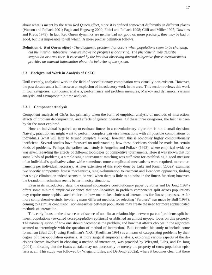
about what is meant by the termRed Queen effect, since it is defined somewhat differently in different places(Watson and Pollack 2001; Pagie and Hogeweg 2000; Ficici andPollack 1998; Cliff and Miller 1995; Dawkinsand Krebs 1979). In fact, Red Queen dynamics are neither bad nor good or, more precisely, theymaybe bad orgood, but it is impossible to tell which. A more precise definition follows.

Definition 6. Red Queen effect- The diagnostic problem that occurs when populations seem to be changing,but the internal subjective measure shows no progress is occurring. The phenomena may describestagnation or arms race. It is created by the fact that observing internal subjective fitness measurementsprovides no external information about the behavior of the system.

2.3 Background Work in Analysis of CoEC

Until recently, analytical work in the field of coevolutionary computation was virtually non-existent. However,the past decade and a half has seen an explosion of introductory work in the area. This section reviews this workin four categories: component analysis, performance and problem measures, Markov and dynamical systemsanalysis, and asymptotic run time analysis.

2.3.1 Component Analysis

Component analysis of CEAs has primarily taken the form of empirical analysis of methods of interaction,effects of problem decomposition, and effects of genetic operators. Of these three categories, the first has beenby far the most explored.

How an individual is paired up to evaluate fitness in a coevolutionary algorithm is not a small decision.Naively, practitioners might want to perform complete pairwise interactions with all possible combinations ofindividuals (what will later be termedcomplete mixing); however, this is obviously highly computationallyinefficient. Several studies have focussed on understanding how these decisions should be made for certainkinds of problems. Perhaps the earliest such study is Angeline and Pollack (1993), where empirical evidencewas given regarding the effects of different topologies of competitive tournaments. Here it was shown that forsome kinds of problems, a simple single tournament matchingwas sufficient for establishing a good measureof an individual’s qualitative value, while sometimes morecomplicated mechanisms were required, more tour-naments per individual necessary. A later extension of thisstudy done by Luke and Panait (2002a) examinestwo specific competitive fitness mechanisms, single-elimination tournament andk-random opponents, findingthat single elimination indeed seems to do well when there islittle to no noise in the fitness function; however,thek-random mechanism seems better in noisy situations.

Even in its introductory state, the original cooperative coevolutionary paper by Potter and De Jong (1994)offers some minimal empirical evidence that non-linearities in problem components split across populationsmay require more sophisticated choices in how one makes choices of interactions for fitness purposes. A farmore comprehensive study, involving many different methods for selecting “Partners” was made by Bull (1997),coming to a similar conclusion: non-linearities between populations may create the need for more sophisticatedmethods of interaction.

This early focus on the absence or existence of non-linear relationships between parts of problems split be-tween populations (so-calledcross-population epistasis) established an almost myopic focus on this property.The natural question of how one should decompose the problem, and how that affects choices in the algorithmseemed to intermingle with the question of method of interaction. Bull extended his study to include someformalism (Bull 2001) using Kauffman’s NKC (Kauffman 1991)as a means of categorizing problems by theirdegree of cross-population epistasis. A more surgical empirical analysis, exploring various aspects of the de-cisions factors involved in choosing a method of interaction, was provided by Wiegand, Liles, and De Jong(2001), indicating that the issues at stake may not necessarily be merely the property of cross-population epis-tasis at all. This study was followed by Wiegand, Liles, and De Jong (2002a), where it becomes clear that there

18

are differenttypesof epistasis that can have different impacts on this decision. Both of these studies form thebasis a some of the research discussed in chapter 3.

In his 1997 dissertation, Potter (1997) conducts a small empirical study to attempt to understand the effectsof static problem decomposition by analyzing a string matching problem, in which the degree of overlap of thematch is controlled for the study. This study suggests very little save that, for some problems, even with strongoverlap his general CCEA framework can still work reasonably well. A year later, Bull published a companionarticle to the above cited article on “partnership”, where he showed that the effects of mutation on CEAs canalso be quite sensitive to problem properties (Bull 1998).

2.3.2 Performance and Problem Measures

Perhaps the first work attempting to establish a method for external (though still subjective) measurement ofCEAs was Cliff and Miller (1995), where a method using the history of the run itself is employed to helptrack and diagnose dynamics in CEAs. An information-theoretic approach was used by Ficici and Pollack(1998) in order to provide a measure that is both external andobjective for the purposes of such diagnostics.This method helped them determine how, in certain settings,arms race behaviors might be established. Morerecently, Stanley and Miikkulainen (2002) developed an external, subjective measure based on dominance thatcan be useful for comparing two different CEAs, but may provide less useful information about the types ofdynamics exhibited in each.

In addition, several empirical studies also attempted to compare search dynamics between CEAs and tradi-tional EAs using problems with implicit external measures (Pagie and Mitchell 2001; Juille and Pollack 1998),showing that arms race dynamics can often be quite tricky to establish, and that population structure choices(such as spatial embedding) may be of some help. Watson and Pollack (2001) establishes a precedent for usinga very simple problem medium in order to understand evolutionary dynamics, which was followed by a muchmore formal study by Bucci and Pollack (2003) illustrating that many types of coevolutionary problems canbe reduced to this simple medium, and that the problem of focussing may be more common than many CoECresearchers believe.

The above work was based on an order-theoretic approach for helping to define problems that are in somesense intrinsically coevolutionary (Bucci and Pollack 2002). Luke and Wiegand (2002), another formal study,also shows that the order relationships in problem’s rewardsystem can suggest characteristics about the dy-namics, indicating that in certain cases coevolutionary dynamics in single-population CEAs can be equivalentto traditional EA dynamics. In addition to these works, Olsson (2001) provides an analysis that suggests thatasymmetries in coevolutionary problems can have profound effects on their dynamical behaviors.

Not only has analysis been done to help understand and diagnose dynamical behaviors in CEAs, but somelimited amount of effort has been employed to try to make use of that knowledge in improving the search,such as the afore mentioned Ficici and Pollack (1998) paper.Additionally, Rosin and Belew (1997, Rosinand Belew (1995) suggest mechanisms such as “hall of fame”, “competitive shared fitness”, and “shared sam-pling”, harnessed through a rough form of static equilibriaanalysis, to help improve coevolutionary search byproviding a higher probability of finding adequate “teaching sets”. In addition to this approach, Ficici and Pol-lack (2001) considers the overlap between multi-objectiveproblem characteristics and coevolutionary problemcharacteristics to use the notion of Pareto optimality to help improve coevolutionary search.

2.3.3 Markov and Dynamical Systems Analysis

Dynamical systems approaches constitute perhaps the most promising category of theoretical analysis of coevo-lutionary algorithms. These models have primarily become popular as a result of two, related influences. Thefirst source of inspiration comes from the fields of biology and economics, where the notions of evolutionarygame theory (EGT) (Hofbauer and Sigmund 1998; Weibull 1992;Maynard-Smith 1982) have helped illustratedynamical, “evolutive” (steady-state, in the dynamical systems sense) (Osborne and Rubinstein 1998) behaviors

19

of systems that are very similar to coevolutionary systems.The second source is from within the EC commu-nity itself, where dynamical systems models have become increasingly more popular tools for understandingthe dynamical properties of EAs (Reeves and Rowe 2002; Vose 1999).

The early EGT model model introduced by Maynard-Smith was originally applied, with little success, toattempt to predict behaviors in an EA by Fogel, Andrews, and Fogel (1998, Fogel, Fogel, and Andrews (1995,Fogel and Fogel (1995). However, these studies were somewhat remiss with how they matched the assumptionsof the model with those of the algorithms being modeled. Ficici and Pollack (2000a), in an effort to re-applythis method, was able to match behaviors of real algorithms to the model predictions much better than theseearlier works. Moreover, Ficici and Pollack (2000c) can perhaps be credited with offering the first real promiseof using EGT for understanding dynamical behaviors in CEAs,from which it has been learned that certaintypes of traditional selection methods may be pathologicalin certain single population EAs (Ficici and Pollack2000b). This EGT model was then turned towards cooperative CEAs (Wiegand, Liles, and De Jong 2002b;Wiegand, Liles, and De Jong 2002a), where it begins to becomeclear that the dynamical properties of CCEAsmay not be as simple as previously believed. Extensions and refinements to this work constitute a large portionof this dissertation.

In very recent years, use of these dynamical systems approaches for coevolution has begun to become quiteprevalent. Quite independently of the EGT work, efforts by Schmitt (2001) apply Markov modeling methodsto EAs in which the fitness of individuals is population dependent, including competing agents under the con-ditional that an overall dominant strategy exists. Again, independent of the above work, Subbu and Sanderson(2000) uses a dynamical systems model with an altogether different framework in order to analyze distributedcooperative coevolutionary algorithms. This work, while being heavily entrenched in assumptions regardingGaussian mutation operators and Gaussian-type problem properties, demonstrates surprisingly powerful resultsregarding the convergence properties of such algorithms. Also, recent work by Liekens, Eikelder, and Hilbers(2003) has applied Markov modeling techniques as a means of comparing CEAs, and in fact performs suchan analysis as a means to understand the benefits of diploidy in coevolution. Additionally, Schmitt (2003) hasfurther developed his Markov model for EAs to include certain kinds of CEAs.

2.3.4 Asymptotic Run Time Analysis

Though still in the very early stages, some recent research incorporates more traditional computer scienceasymptotic analytical methods, such as those applied toward other types of randomized algorithms (Motwaniand Raghavan 2000). Jansen and Wiegand (2003b) presents therun time performance of a very simple co-operative coevolutionary algorithm on several separable problem classes in terms of expected time before theglobal optimum is reached first. This research again casts doubt on the older belief that cooperative coevolutiongains advantage when there is little or no non-linear relationships between pieces of the problem representedby different populations. I will cover such analyses in greater detail in Chapter 4. Further analysis of this sortwas applied by Jansen and Wiegand (2003c) to illustrate differences between two different implementations ofa simple CCEA, one parallel and one sequential in terms of howthe current populations are updated. This studysuggests that the differences and similarities between such implementations are, perhaps, counter intuitive.

Chapter 3

Coevolutionary Architectures

In the previous chapter, I introduced a tentative definitionof a coevolutionary algorithm: an evolutionary al-gorithm in which the fitness of an individual is a subjective function of its interactions with other individuals.An exact definition of just precisely what is, or is not, coevolution will not be offered; however, in order tostudy something, one must certainly clarify the object of study itself. This chapter seeks to do exactly this:lay the groundwork for understanding the specific class of coevolutionary algorithms on which this dissertationfocusses.

The chapter begins this clarification by first offering a categorical description of the properties of CEAs.This has the double advantage of informing the reader of choices available to CoEC designers, while alsoproviding a context for understanding the choices made for this particular set of studies. With this beginning,the second section is able to position theCooperative Coevolutionary Algorithm(CCEA) framework understudy here within the larger hierarchy of CEAs in general. Since the point of my fundamental question centersaround the notion of static optimization, the third sectionseeks to clarify this problem domain for the CCEA.The result of this chapter should be a clear understanding ofthe algorithm I am studying and the problem towhich some seek to apply it.

3.1 Categorizing Coevolutionary Algorithms

Just as with more traditional EAs, there are many design choices available to engineers employing coevolu-tionary algorithms. Different choices lead to different CEAs with different properties; thus, it is in a designer’sbest interest to understand these choices. Some of the choices have already been touched upon in the previouschapter, but it is useful to provide a systematic, hierarchical elicitation of them in greater detail. Indeed, thissection offers a categorical ontology of coevolutionary algorithms, based on the choices available to algorithmdesigners. The descriptions of these categories follow Figure 3.1 on page 23, which provides a roadmap forthese descriptions.

A categorization such as this is necessary if one is to take a systematic approach to understanding coevo-lution. Any given analysis of a class of coevolutionary algorithms can be made more clear (and specific) bydirectly addressing which subset of properties are explored in that analysis. Knowing a reasonably thoroughontological breakdown of properties helps researchers andpractitioners understand what the generalities, aswell as what the limitations, of such an analysis must be. Moreover, once a broad range of properties is moreobvious in some holistic sense (as is hopefully the case withthe hierarchy on page 23), more focussed and sen-sible analytical processes are possible by establishing a context. Additionally, a better understanding of whatisnot covered in prevailing research is illumined in this way.

As we will soon see, there is a large amount of semantic ambiguity surrounding many coevolutionaryalgorithms that make them difficult to classify. This difficulty only increases the need for some kind of catego-rization. By describing the various choices that go into defining a coevolutionary algorithm, the places wherethese ambiguities are the highest will be made more explicit.

As you can see from the figure on page 23, there are at least two high level branches to choices aboutcoevolutionary algorithms: choices centering around how one evaluates fitness in a CEA and choices centering

21

22

around how one represents the problem for the algorithm to solve. The following subsections offer shortdescriptions of each of these, and their subcategories, in turn.

3.1.1 Evaluation

Since CEAs are defined by the fact that their internal measure, or evaluated fitness, is a subjective measure, alogical breakdown of defining properties for CEAs should include evaluation as a high level category. Indeed,there are at least four different properties of evaluation important to coevolution: payoff quality, methods offitness assignment, methods of interaction, and update timing. Though there may be other important propertiesof CEA evaluation, these four must certainly be the most significant, and within these categories nearly allexisting CoEC approaches can be described.

Payoff Quality

The first broad category of coevolutionary algorithm evaluation surrounds the character of the payoffs awardedduring interaction of individuals. This is essentially a tacit reference to the game-theoretic nature of coevolutionthat I will discuss later in the thesis. The basic question is: if one is evaluating interactions, how are theseinteractions best characterized? There are at least three payoff types in CEAs worth considering: competitivefitness, cooperative fitness, and non–competitive fitness. The reader should be careful to note that these aretraditional, qualitative classifications that leave a lot of grey area to be disambiguated. In fact, there is muchdisagreement about the scope and relevance of these grey areas within the field of CoEC. I will return to thisquestion of ambiguity below, but first let’s say a few words about the categories themselves.

In competitive coevolution, individuals are rewarded when their opponents do poorly, and they are punishedwhen their opponents do well. In other words, their fitness values depend oncompetitions, and the individualsparticipating in these competitions are consideredcompetitorsor opponents.

Alternatively, in cooperative coevolutionthe fitness of an individual is based on how well it cooperateswith the other individuals with whom it interacts. Individuals succeed when they are partnered well, when theresulting team performs well. Here I term the interaction itself acollaboration, and use the termcollaboratorto mean those individuals with which the interaction is made.

Though the definitions offered for distinguishing between cooperative and competitive coevolutionarymethods remain somewhat vague, one thing that is clear is that one can imagine payoff situations where some-times participants are mutually rewarded, but sometimes their purposes are at odds. Such situations are oftenreferred to asnon–competitive. This thesis will ignore non–competitive approaches sincethey are (so far) oflittle interest to those who study CEAs at this time. Nevertheless, it should be clear that it may well be thelargest of the three groups.

Returning to my point about the ambiguity of these definitions, the question of how to clearly define thesegroups of payoff quality is a very messy and complicated semantic problem. There’s little doubt that moreprecise, mathematically rigorous definitions of the distinction between cooperation and competition may wellbe helpful. Indeed, such distinctions may be plausibly obtained using the notational tools from game theory(Rapoport 1970); however, the differences of opinions among CoEC researchers currently regarding subtletiesof what is meant by these terms makes any unilateral attempt to draw a hard defining line between cooperativeand competitive coevolution unwise. This dissertation, therefore, will not attempt to do so. Instead, as will beseen later in this chapter, the studies presented here will restrict their attention to a subset of such models thatare undeniably cooperative.

Perhaps of more fundamental interest than terminological distinctions, may be whether or not any particularcharacterization of this sort has any meaning in terms of identifying potential long term dynamics in a coevo-lutionary system. This remains an open question, though theconnection between payoff quality and long termcoevolutionary behaviors is widely believed to exist (Ficici and Pollack 2000c).

23

Evaluation

PayoffQuality

Cooperative

Competitive

Non-Competitive

Methods ofFitnessAssignment

Implicit

Explicit

Methods ofInteraction

Sample Size

Selective Bias

Credit Assignment

UpdateTiming

Sequential

Parallel

Representation

ProblemDecomposition

PartitioningMethods

DecompositionalTemporality

Static

Dynamic

Adaptive

SpatialTopology

Spatial Embedding

Non-Spatial Embedding

PopulationStructure

Single

Multiple

Figure 3.1: Hierarchical categorization of CEA properties.

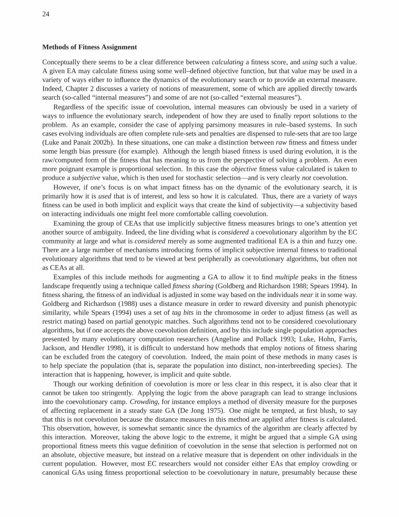
24

Methods of Fitness Assignment

Conceptually there seems to be a clear difference betweencalculatinga fitness score, andusingsuch a value.A given EA may calculate fitness using some well–defined objective function, but that value may be used in avariety of ways either to influence the dynamics of the evolutionary search or to provide an external measure.Indeed, Chapter 2 discusses a variety of notions of measurement, some of which are applied directly towardssearch (so-called “internal measures”) and some of are not (so-called “external measures”).

Regardless of the specific issue of coevolution, internal measures can obviously be used in a variety ofways to influence the evolutionary search, independent of how they are used to finally report solutions to theproblem. As an example, consider the case of applying parsimony measures in rule–based systems. In suchcases evolving individuals are often complete rule-sets and penalties are dispensed to rule-sets that are too large(Luke and Panait 2002b). In these situations, one can make a distinction betweenraw fitness and fitness undersome length bias pressure (for example). Although the length biased fitness is used during evolution, it is theraw/computed form of the fitness that has meaning to us from the perspective of solving a problem. An evenmore poignant example is proportional selection. In this case theobjectivefitness value calculated is taken toproduce asubjectivevalue, which is then used for stochastic selection—and is very clearlynot coevolution.

However, if one’s focus is on what impact fitness has on the dynamic of the evolutionary search, it isprimarily how it isusedthat is of interest, and less so how it is calculated. Thus, there are a variety of waysfitness can be used in both implicit and explicit ways that create the kind of subjectivity—a subjectivity basedon interacting individuals one might feel more comfortablecalling coevolution.

Examining the group of CEAs that use implicitly subjective fitness measures brings to one’s attention yetanother source of ambiguity. Indeed, the line dividing whatis considereda coevolutionary algorithm by the ECcommunity at large and what isconsideredmerely as some augmented traditional EA is a thin and fuzzy one.There are a large number of mechanisms introducing forms of implicit subjective internal fitness to traditionalevolutionary algorithms that tend to be viewed at best peripherally as coevolutionary algorithms, but often notas CEAs at all.

Examples of this include methods for augmenting a GA to allowit to find multiple peaks in the fitnesslandscape frequently using a technique calledfitness sharing(Goldberg and Richardson 1988; Spears 1994). Infitness sharing, the fitness of an individual is adjusted in some way based on the individualsnear it in some way.Goldberg and Richardson (1988) uses a distance measure in order to reward diversity and punish phenotypicsimilarity, while Spears (1994) uses a set oftag bits in the chromosome in order to adjust fitness (as well asrestrict mating) based on partial genotypic matches. Such algorithms tend not to be considered coevolutionaryalgorithms, but if one accepts the above coevolution definition, and by this include single population approachespresented by many evolutionary computation researchers (Angeline and Pollack 1993; Luke, Hohn, Farris,Jackson, and Hendler 1998), it is difficult to understand howmethods that employ notions of fitness sharingcan be excluded from the category of coevolution. Indeed, the main point of these methods in many cases isto help speciate the population (that is, separate the population into distinct, non-interbreeding species). Theinteraction that is happening, however, is implicit and quite subtle.

Though our working definition of coevolution is more or less clear in this respect, it is also clear that itcannot be taken too stringently. Applying the logic from theabove paragraph can lead to strange inclusionsinto the coevolutionary camp.Crowding, for instance employs a method of diversity measure for the purposesof affecting replacement in a steady state GA (De Jong 1975).One might be tempted, at first blush, to saythat this is not coevolution because the distance measures in this method are applied after fitness is calculated.This observation, however, is somewhat semantic since the dynamics of the algorithm are clearly affected bythis interaction. Moreover, taking the above logic to the extreme, it might be argued that a simple GA usingproportional fitness meets this vague definition of coevolution in the sense that selection is performed not onan absolute, objective measure, but instead on a relative measure that is dependent on other individuals in thecurrent population. However, most EC researchers would notconsider either EAs that employ crowding orcanonical GAs using fitness proportional selection to be coevolutionary in nature, presumably because these

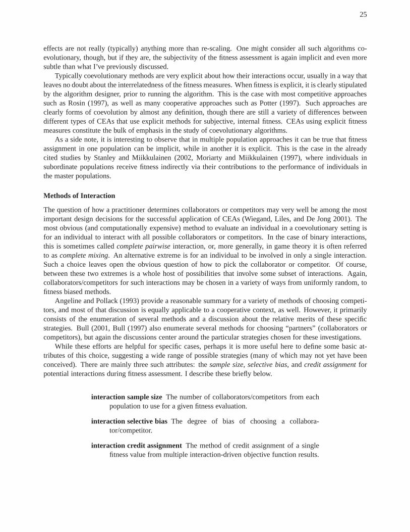
25

effects are not really (typically) anything more than re-scaling. One might consider all such algorithms co-evolutionary, though, but if they are, the subjectivity of the fitness assessment is again implicit and even moresubtle than what I’ve previously discussed.

Typically coevolutionary methods are very explicit about how their interactions occur, usually in a way thatleaves no doubt about the interrelatedness of the fitness measures. When fitness is explicit, it is clearly stipulatedby the algorithm designer, prior to running the algorithm. This is the case with most competitive approachessuch as Rosin (1997), as well as many cooperative approachessuch as Potter (1997). Such approaches areclearly forms of coevolution by almost any definition, though there are still a variety of differences betweendifferent types of CEAs that use explicit methods for subjective, internal fitness. CEAs using explicit fitnessmeasures constitute the bulk of emphasis in the study of coevolutionary algorithms.

As a side note, it is interesting to observe that in multiple population approaches it can be true that fitnessassignment in one population can be implicit, while in another it is explicit. This is the case in the alreadycited studies by Stanley and Miikkulainen (2002, Moriarty and Miikkulainen (1997), where individuals insubordinate populations receive fitness indirectly via their contributions to the performance of individuals inthe master populations.

Methods of Interaction

The question of how a practitioner determines collaborators or competitors may very well be among the mostimportant design decisions for the successful applicationof CEAs (Wiegand, Liles, and De Jong 2001). Themost obvious (and computationally expensive) method to evaluate an individual in a coevolutionary setting isfor an individual to interact with all possible collaborators or competitors. In the case of binary interactions,this is sometimes calledcomplete pairwiseinteraction, or, more generally, in game theory it is often referredto ascomplete mixing. An alternative extreme is for an individual to be involved in only a single interaction.Such a choice leaves open the obvious question of how to pick the collaborator or competitor. Of course,between these two extremes is a whole host of possibilities that involve some subset of interactions. Again,collaborators/competitors for such interactions may be chosen in a variety of ways from uniformly random, tofitness biased methods.

Angeline and Pollack (1993) provide a reasonable summary for a variety of methods of choosing competi-tors, and most of that discussion is equally applicable to a cooperative context, as well. However, it primarilyconsists of the enumeration of several methods and a discussion about the relative merits of these specificstrategies. Bull (2001, Bull (1997) also enumerate severalmethods for choosing “partners” (collaborators orcompetitors), but again the discussions center around the particular strategies chosen for these investigations.

While these efforts are helpful for specific cases, perhaps it is more useful here to define some basic at-tributes of this choice, suggesting a wide range of possiblestrategies (many of which may not yet have beenconceived). There are mainly three such attributes: thesample size, selective bias, andcredit assignmentforpotential interactions during fitness assessment. I describe these briefly below.

interaction sample sizeThe number of collaborators/competitors from eachpopulation to use for a given fitness evaluation.

interaction selective biasThe degree of bias of choosing a collabora-tor/competitor.

interaction credit assignment The method of credit assignment of a singlefitness value from multiple interaction-driven objective function results.

26

Since how one makes such choices may be of high import to practitioners, much of the empirical researchconducted by this thesis in Chapter 4 will center around determining how such choices affect the performanceof existing coevolutionary algorithms. There may be other properties of this decision, but none so salient asthese three.

Update Timing

Introducing multiple populations into an EA brings to the table some necessary clarifications about terminology.For example, some clarity with respect to the wordgenerationis required. In a traditional generational EA, thistypically refers one complete pass through the parent selection, offspring generation, evaluation, and survivalselection (steps 4.1–4.5 in Algorithm 1 on page 8). I will retain this term in exactly this way for coevolution.That is, agenerationin a CCEA is the time it takes to move through these steps for a single population. To referto the complete cycle of processing all populations, I use the termround1.

Next, do collaborators come from the current state of populations, or from populations from the previousround? Really this is a question of the timing of when populations are processed and updated. The timing ofsuch things can be done in a variety of ways; I focus on two.

I use the termsequentialto refer to a coevolutionary algorithm that processes each population in a sequentialorder, choosing collaborators from the current state of theother populations. These populations can changeduring theround, of course. As a result, populations processed and updated earlier in the round can affect theprocessing of populations processed later.

An alternate approach is one in which the individual populations are processed inparallel, synchronizedonly at the end of each round. In this approach, collaborators are selected from theprevious generationfromeach population. A clearer description of the differences between these two approaches can be obtained inJansen and Wiegand (2003c).

3.1.2 Representation

There are three particularly important groups of representation-oriented decisions that design engineers mustmake when implementing CEAs: how one handles problem decomposition, what is the spatial topology, andhow one structures the population(s). Among these three categories, nearly all CEAs can be described one wayor the other, though not all CEAs rely as heavily on some of these properties as do others.

Problem Decomposition

For cooperative coevolution in particular, it is often necessary to decide how a larger problem will be decom-posed into smaller components. There are many ways one may perform this task; such methods fall into acategory here calledpartitioning methods. Chapter 4 will explore the issue of partitioning methods and theireffects more carefully.

The next question iswhenthis decomposition occurs. Just like any parameter adjustment, the property ofdecompositional temporalitymay bestatic, decided once and for alla priori by the design engineer;dynamic,adjusted during run time using a rule imposed by the design engineera priori; andadaptive, adjusted duringrun time by the system itself. The idea behind this distinction is similar to more traditional EA choices withrespect to how parameters are altered (or not) at run time (Eiben and Michalewicz 1998; Angeline 1995).

The challenge of how and when to decompose a problem for the purposes of coevolving the individual com-ponents is one of the most important questions facing CoEC researchers. In fact, the nature of these decisionson the part of design engineers poses unique questions regarding the appropriateness of decomposition in termsof the true structure of the problem at hand. Since these may be very appropriate, or distinctly inappropriate, aswill be seen later in the dissertation, it is important to make informed choices. Due to the difference between a

1I prefer thegeneration/roundterminology to that offered by Potter (1997):generationversusecosystem generation.

27

decomposition made by the representation and the natural decomposition of the problem, I use the termcom-ponentto mean a part of a representation, given by the algorithm, while I use the termpieceto mean portionsof the problem itself.

Spatial Topology

Fine-grained, distributed representations of populations are important categories of traditional EAs (Sarma andDe Jong 1996), but they are also quite important in coevolutionary algorithms, since they beg the additionalquestion of how multiple populations relate to one another topologically (Pagie and Hogeweg 2000). Indeed,some early research has suggested that spatially-embeddedCEAs might outperform non-spatial methods onsome problems, in certain confined circumstances.

Of course, the bulk of CEAs use no such spatial embedding, buta modest subset of application orientedwork now involves these fine-grained approaches. The research on such models, as well as its apparent potentialadvantage, suggests that this category should appear in ourontology. Design choices for fine-grained CEAsare complicated, but are for the most part outside the scope of this work. This dissertation distinguishes onlybetween models that arespatially embeddedand those that arenon-spatially embedded. It should be noted,however, that topological relationships in spatially embedded models are inherently connected to methods ofinteraction in terms of evaluation.

Population Structure

There are many ways for a design engineer to break up a coevolutionary algorithm; however, the primarydistinction made here is whethermultiple populationsor a single populationis employed by a given CEA.These two mark off very different areas of coevolutionary research, so this division constitutes a highly usefuldistinction.

For our purposes, let us assume that in single population approaches individuals interact with other indi-viduals within the same population for obtaining fitness, while in multiple population approaches individualsinteract only with individuals fromother populations to obtain fitness. While it is possible to consider algo-rithms in which there are interactions between individualsin the same populationand other populations, it isrelatively rare and unhelpful to consider such complications. Indeed, as it turns out, there are apparently someclear distinctions between single and multiple populationapproaches in terms of dynamics (Ficici and Pollack2000c; Hofbauer and Sigmund 1998).

3.2 A Cooperative Coevolutionary Algorithm

In the previous section, I offered a categorical description of the design choices available to those wishing toconstruct coevolutionary algorithms. Using this hierarchy, nearly any conceivable coevolutionary algorithmcan be described, even those that fall into the grey areas of what is considered coevolution. However, to saysomething specific, to answer direct and pointed questions,I must restrict our attention to a subset of CEAs thatare most salient for the purposes of the study at hand.

In my case, every attempt has been made to keep the class of CEAs under study as simple as is possible.The ultimate goal is to preserve the coevolutionary nature of the algorithm, while providing an algorithm thatgives rise to interesting and useful questions. Therefore,some of the choices available to us will be restrictedin the interest of simplicity and focus, while others will bevaried in order to answer practical questions aboutthe class of algorithms considered. To help clarify this more specifically, I will divide my discussion into threeparts. In the first two parts, I describe properties of the algorithm relating to evaluation and representation,respectively. In the final part, I will offer a more detailed description of the algorithms’ framework.

28

3.2.1 Evaluation

While there are certainly interesting questions relating to both cooperative and competitive coevolution, coop-erative coevolution may meet the “simple” criteria somewhat more directly. The lack of a clear external andobjective measure for most competitive methods, in combination with the semantic difficulty defining optimal-ity, makes progress measurement a problem. This creates challenges for study, since often this measurementproblem must be solved before any more analysis can be accomplished. Moreover, existing research suggeststhat the dynamical properties of competitive systems may very well be more challenging to understand thanthose of cooperative systems. Since part of my goal is one of simplification, the algorithms studied in thisdissertation will be explicitly cooperative, in the sense that they meet the qualitative definition of cooperativecoevolution payoff quality and explicit fitness assignmentoffered in the previous section.

However, since one of the key decisions that face cooperative coevolutionary algorithm designers surroundsthe method of interaction, this property will remain variable for our investigations. Indeed, the next chapter willexplore the nature of this choice, and its effects in detail.

This issue of what kind of effects the timing of processing and updating populations has on the CCEA is acomplex one. My analysis here does not include a discussion of the differences, though related work is citedthat does (see Jansen and Wiegand (2003c), for example); however, I will concentrate primarily on sequentialCCEAs in Chapter 4 and on parallel CCEAs in Chapter 5.

Before moving on to discuss representation, it is necessaryto say a few words about the ambiguity of theterm “cooperative” raised in the previous section. In the next section I will describe the problem domains towhich this dissertation restricts its attention, and the definitiveness of the cooperative nature of the algorithmson such problems will be more clear. Despite the general ambiguity in this term, the most obvious and directstatic single-objective optimization tasks suggest a cooperative approach. Since the notion of optimization isat the heart of the fundamental question of the dissertation, it seems to be the most appropriate decision underthese circumstances.

3.2.2 Representation

For reasons of simplicity, the algorithms in this work use only a priori static decompositions, though thepartitioning method will be the subject of some of the research in the next chapter since it relates stronglyto methods of interaction. I primarily will focus on algorithms that are non-spatially embedded; however, inthe final chapter a particular spatial model is used to make a parting point about establishing and maintainingevolutionary balance during the run. The primary research investigations of this thesis focusses entirely onnon-spatial models, though.

Single population models can be quite messy and complicatedto describe and understand. Moreover, itis unclear whether cooperative algorithms are even possible in such a setting, given that it is the nature ofindividuals in a population to compete for selection, regardless of the nature of their interactions. To avoidthis complexity, as well as to place this research safely in the “coevolution” camp, I employ only multiplepopulation approaches in which the fitness of an individual from one population is the result of collaborationswith individuals from each of the other populations.

3.2.3 A General Cooperative Coevolution Framework

The discussion above defines a rather large class of potential CEAs. Unless otherwise stated, from this pointforward the termcooperative coevolutionary algorithm(CCEA) will to refer this particular class of multi-population, cooperative algorithms using explicit fitnessassignment methods and static problem decomposi-tions.

When applying a CCEA to a particular problem, typically one decomposes the problem into componentsand assigns each component to a population. Save for evaluation, each population is evolved more or less inde-pendently of one another. since any given individual from a particular population represents only a component

29

of a potential solution to the problem, collaborators are selected from the other populations to represent theremaining components. The individual is combined with its collaborators to form a complete solution and theobjective function is evaluated. If there is more than one set of collaborators (depending on the collaboratorsample size) for a given individual, the objective functionmay be evaluated many times, but a single score issomehow attributed to the individual for fitness (dependingon the collaborator credit assignment method). Itshould be noted that the populations of a CCEA may or may not behomogeneous with respect to the repre-sentation used for the encoding of individuals in them, or the underlying EAs being used to evolve a particularcomponent. For the sake of simplicity, all the studies in this dissertation will assume a more or less consistentrepresentation across populations. Figure 3.2 on page 30 illustrates this idea pictorially.

This class of CCEAs is in no way new. Indeed, Potter (1997) describes a generalized framework for theCCEA, one that has been applied in a variety of ways. To be morespecific, the traditional EA code shown inFigure 1 on page 8 is extended, describing the abstractsequentialCCEA in the pseudo-code in Figure 2 below.

Algorithm 2 (Abstract Sequential Cooperative Coevolutionary Algorithm).1. for population ps ∈ P, all populations

1.1 Initialize population ps2. for population ps ∈ P, all populations

2.1 Evaluatepopulation ps3. t := 04. do

4.1 for population ps ∈ P, all populations4.1.1Select parentsfrom population ps4.1.2Generate offspringfrom parents4.1.3Select collaboratorsfrom P4.1.4Evaluateoffspring with collaborators4.1.5Select survivorsfor new population Ps

4.2 t := t + 1until Terminating criteria is met.

3.3 Optimizing with The CCEA

In the previous section, I detailed the specific class of algorithms I will be analyzing. Several things remainto be clarified, however. For one thing, there is again the question of to which class of problem domains torestrict attention. The answer to this question arises fromboth the need to meet the fundamental question(Do CCEAs optimize?), as well as meet the condition of being as simple as is possible to demonstrate usefulthings about coevolution. Perhaps the simplest possible domain one might consider for the CCEA is the that ofsingle-objective, static function optimization.

Such problems have at least two properties of interest here.First, they suggest some direct and obviousmethods of decomposition. Second, given fairly straightforward decompositions, they have a game-theoreticproperty that is important to the analysis: symmetry. Before turning to these issues, I will clarify what is meantby single-objective, static function optimization. I focus on maximization. The results and observations areequally applicable to minimization.

Definition 7. Let there be some function, F, over domain D, F: D→R. Asingle-objective, static maximizationproblemis a problem in which the goal is to find d∗ ∈ D such that d∗ = argmaxDF.

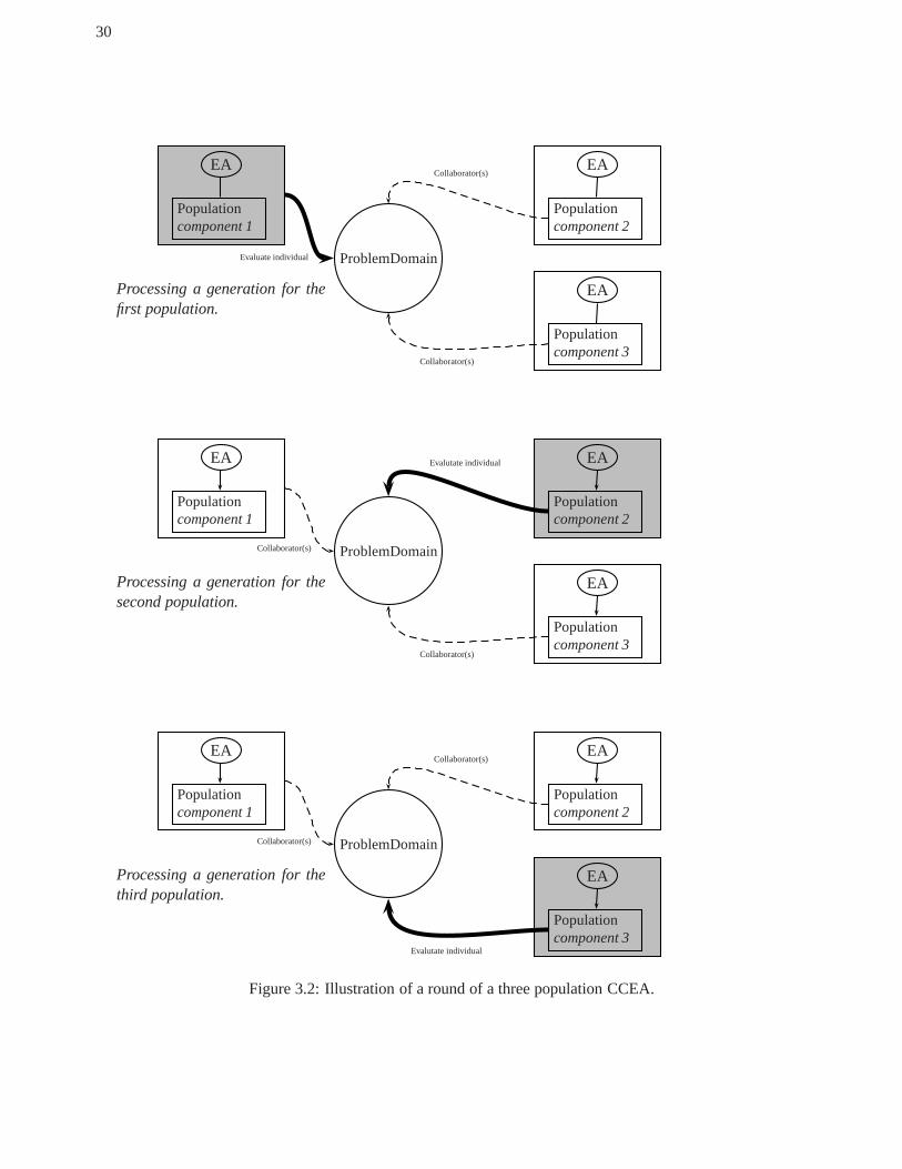
30

EA

Populationcomponent 1

EA


ProblemDomain

EA


Evaluate individual

Collaborator(s)

Collaborator(s)

Processing a generation for thefirst population.

EA


EA


ProblemDomain

EA


Collaborator(s)

Evalutate individual

Collaborator(s)

Processing a generation for thesecond population.

EA


EA


ProblemDomain

EA


Collaborator(s)

Collaborator(s)

Evalutate individual

Processing a generation for thethird population.

Figure 3.2: Illustration of a round of a three population CCEA.

31

3.3.1 Decomposing a Static Function Optimization Problem

The problem class defined above is attractive in part becauseof its simplicity. It is also attractive because despiteits simplicity there remain interesting research issues surrounding how one decomposes the domain such to berepresented by multiple populations. Moreover, since a large number of real world applications fall into thisdomain, answering questions about static optimization provides useful information for practitioners.

In essence, the decomposition issue is a question of how to partition D. Consider, for example, the domainconsisting of a vector of arguments in Euclidean space (~x ∈ R

n). Here each argument of the function mightbe represented by a different population. In such a case, evaluating an individual from the first first popula-tion (argumentx1, for example), requires choosing collaborators from the other populations representing otherarguments (argumentsx2 andx3, for example). Figure 3.3 on page 31 illustrates this case.

x1 x2

f (x1,x2,x3)

x3

Evaluate individual

Collaborator(s)

Collaborator(s)

Figure 3.3: Illustration of how a CCEA might assemble a decomposed real-valued argument list to evaluateagainst a static objective function.

In the case of a binary representation, such a partitioning is most obviously done by dividing the binarystring into different substrings. Individuals in each population might represent a particular partitioned substring,and evaluation of an individual substring will require representation from substrings in other populations. Forexample, Figure 3.4 offers an example to illustrate how a decomposed binary string might be assembled inorder to evaluate it with some objective function. In this particular case, the string is broken up into three equallength segments for each population. This is only one choice. Part of the analysis in the next chapter will dealwith exactly this choice.

0110 1100

f (011011000001)

0001

Evaluate individual

Collaborator(s)

Collaborator(s)

Figure 3.4: Illustration of how a CCEA might assemble a decomposed binary to evaluate against a staticobjective function.

32

3.3.2 Symmetry

The field of game theory (GT) has a useful notion ofsymmetrywith respect to games. In this context, asymmetric game is one in which the reward gained for a particular set of strategies, as defined by each playerpicking a specific strategy, will be the same, regardless of which player is currently being considered. Forexample, if one player plays strategya and the other player plays strategyb, the rewards to players depend onlyon a andb, but not on the identities of the players.

On a more mathematical level, letπ : S×S→ R define a function mapping strategies from each of twoplayers to a payoff value. Letπ1(a,b) be the payoff for player 1 when player 1 plays strategya and player 2playsb, andπ2(a,b) be the payoff for player 2. When a game is symmetric,π1(b,a) = π2(a,b).

Having the property of symmetry certainly simplifies a game in many ways. It is exactly this simplificationthat makes it a good property to consider when looking at things from first principles. It should be clear that thepartitioning methods discussed in the previous subsectionwill yield problems with such a property. In essence,the class of CCEAs in which I am interested is symmetric when applied to single-objective, static optimizationproblems, as defined above.

This property has several benefits. First, it should now be clear that the multiple population CCEA definedabove as applied to problems with this property of symmetry are cooperative, by virtually any reasonable defi-nition. A population (player) cannot succeed unless his collaborators (partners) also succeed, and it fails whenthey fail. Second, because of this property of symmetry, a clear objective measure is possible. Since the goalis to optimize the function and the rewards are symmetric, there is no red queen problem because any progressagainst the external measure (the given problem)is, by definition, objective. This resolves several of the ana-lytical challenges observed in so far and leaves me with a simple coevolutionary system and a straightforwardobjective: single-objective static maximization.

Chapter 4

CCEAs as Static Optimizers

Is this class of multi-population, symmetric cooperative coevolutionary algorithms useful as a class of functionoptimizers? In some philosophical sense, all algorithms are optimizers when they are applied to optimizationproblems; they may simply be quite poor optimizers, yielding low quality solutions or taking a far longer timeto find the optimum than other, better suited algorithms might. Perhaps it is unhelpful to wax philosophic: if oneapplies the algorithms to optimization problems, they are optimizers, and our issue (as scientists and engineers)is how they perform and how well they function. Perhaps the “fundamental question” posed in Chapter 1, whilewell-intentioned, is misphrased.

In this chapter, I take this exact approach and rephrase the fundamental question to ask “How, and howwell, do CCEAs act as function optimizers?” Of course, this is a very broad question, with questionable specificresearch potential, so it must be further refined to offer more specific opportunities to provide explicative results.I do this by concentrating on understanding what makes function optimization problems difficult for CCEAs,and what algorithmic design decisions might be used to counter these difficulties. By giving the fundamentalquestion context in this way, one can apply analytical and empirical tools to get more specific, useful answersthan might otherwise be possible.

The chapter begins by first discussing how CCEAs can be applied to the problem domain of static functionoptimization defined in the previous chapter. This section takes up a property commonly believed to cause dif-ficulties for CCEAs (cross-population epistasis), defines this property, and describes the intuition and historicalissues that have lead to the suppositions surrounding its effect on CCEAs. The section that follows describeswhat elements of CCEAs might plausibly lead to coevolutionary advantage over traditional EAs, then exploresthis advantage in the context of cross-population epistasis. This is done by conducting theoretical investigationsof very simple CCEAs, as well as empirical analysis of the operators involved in somewhat more complicatedCCEAs. The third section of the chapter examines what is perhaps the most principal component of CCEAsto deal with challenges posed by complicated problem domains: methods of interaction (collaboration). Thisis done via primarily empirical means. I use the final sectionto bridge to the next chapter by illustrating, bothempirically and formally, some of the challenges that face CCEAs when they are applied to static optimizationproblems.

4.1 Applying CCEAs

4.1.1 General Problem Domain Framework

Before beginning any analysis of the algorithm of study, oneshould be careful to select a framework for theproblem domain that facilitates analysis at some level. Such a domain should be simple enough to gain appro-priate intuition, but flexible enough to allow for a thoroughexploration of the relevant properties of interest. Tothis end, this section concentrates entirely on so–calledpseudo-booleanfunctions, f : 0,1n → R. Individualswill therefore maintain binary representations throughout this chapter. The use of binary representation (in thiscase) provides a greater intuition about the effects of the genetic operators—something that will come in handyduring analysis.

Pseudo-boolean functions provides several additional advantages. First and foremost, they will make it very

33

34

easy to describe the salient problem property that constitutes the focus of the research discussed in this section.Second, they make it very straightforward to construct examples (or counter examples) illustrating certain veryexplicit ideas relating to properties of the problem. Finally, the issue of how well suited a static decompositionis for the overall problem representation becomes simplified by the ease with which clear definitions of suchpartitioning may be established.

Basic Example Functions

Since they will be useful throughout this chapter, several simple pseudo-Boolean functions are defined below:ONEMAX , LEADINGONES, and TRAP. These are very common EA problems (Mitchell 1997). ONEMAX

simply counts the number of ones in a given binary string, LEADINGONES counts the number of consecutiveones at the start of a string, and TRAP essentially establishes a false ONEMAX gradient leading away from thetrue maximum, found at the all 0 string. These are defined formally below.

Definition 8. The functionONEMAX : 0,1n → R is defined by

ONEMAX (x) :=n∑

i=1

xi

.

Definition 9. The functionLEADINGONES: 0,1n → R is defined by

LEADINGONES(x) :=n∑

i=1

i∏

j=1

x j

.

Definition 10. The functionTRAP: 0,1n → R is defined by

TRAP(x) :=

(

(n+1) ·n∏

i=1

xi

)

+n−ONEMAX(x)

.

Using these simple functions, somewhat more complicated functions can be constructed. In fact theONEMAX problem can be seen as a specific case of so-called LINEAR functions. Additionally, it is possi-ble to generalize the LEADINGONES problem to one in which onlyb blocks ones may be counted at the startof the string, LOBb (Jansen and Wiegand 2003a). The following definitions for these two problem classes areoffered below.

Definition 11. The functionONEMAX : 0,1n → R, and some vector w∈ Rn is defined by

L INEAR(x) :=n∑

i=1

wixi

.

Definition 12. For n∈ N and b∈ 1, . . . ,n with n/b∈ N, the functionLOBb : 0,1n → R (short forLeadingOnesBlocks) is defined by

LOBb(x) :=n/b∑

i=1

b·i∏

j=1

x j

.

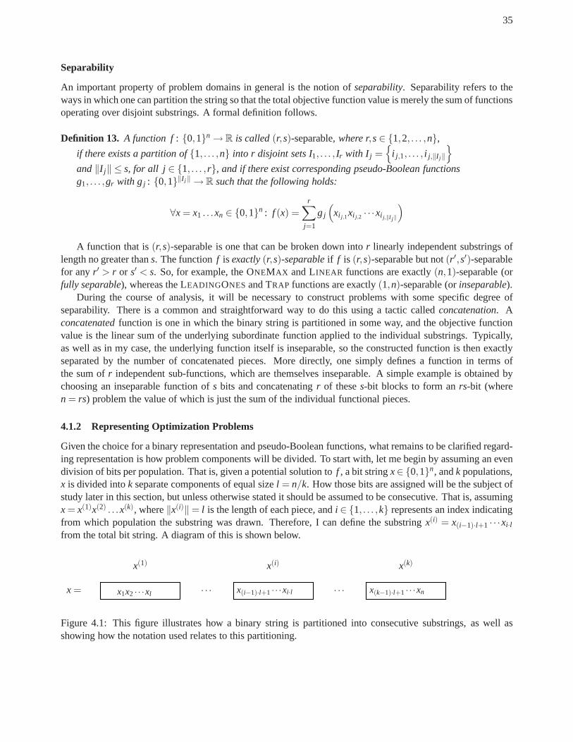
35

Separability

An important property of problem domains in general is the notion of separability. Separability refers to theways in which one can partition the string so that the total objective function value is merely the sum of functionsoperating over disjoint substrings. A formal definition follows.

Definition 13. A function f: 0,1n → R is called(r,s)-separable, where r,s∈ 1,2, . . . ,n,

if there exists a partition of1, . . . ,n into r disjoint sets I1, . . . , Ir with I j =

i j,1, . . . , i j,‖I j‖

and‖I j‖ ≤ s, for all j ∈ 1, . . . , r, and if there exist corresponding pseudo-Boolean functionsg1, . . . ,gr with gj : 0,1‖I j ‖ → R such that the following holds:

∀x = x1 . . .xn ∈ 0,1n : f (x) =r∑

j=1

g j

(

xi j,1xi j,2 · · ·xi j,‖I j ‖

)

A function that is(r,s)-separable is one that can be broken down intor linearly independent substrings oflength no greater thans. The functionf is exactly(r,s)-separableif f is (r,s)-separable but not(r ′,s′)-separablefor any r ′ > r or s′ < s. So, for example, the ONEMAX and LINEAR functions are exactly(n,1)-separable (orfully separable), whereas the LEADINGONES and TRAP functions are exactly(1,n)-separable (orinseparable).

During the course of analysis, it will be necessary to construct problems with some specific degree ofseparability. There is a common and straightforward way to do this using a tactic calledconcatenation. Aconcatenatedfunction is one in which the binary string is partitioned in some way, and the objective functionvalue is the linear sum of the underlying subordinate function applied to the individual substrings. Typically,as well as in my case, the underlying function itself is inseparable, so the constructed function is then exactlyseparated by the number of concatenated pieces. More directly, one simply defines a function in terms ofthe sum ofr independent sub-functions, which are themselves inseparable. A simple example is obtained bychoosing an inseparable function ofs bits and concatenatingr of theses-bit blocks to form anrs-bit (wheren = rs) problem the value of which is just the sum of the individual functional pieces.

4.1.2 Representing Optimization Problems

Given the choice for a binary representation and pseudo-Boolean functions, what remains to be clarified regard-ing representation is how problem components will be divided. To start with, let me begin by assuming an evendivision of bits per population. That is, given a potential solution to f , a bit stringx∈ 0,1n, andk populations,x is divided intok separate components of equal sizel = n/k. How those bits are assigned will be the subject ofstudy later in this section, but unless otherwise stated it should be assumed to be consecutive. That is, assumingx= x(1)x(2) . . .x(k), where‖x(i)‖ = l is the length of each piece, andi ∈ 1, . . . ,k represents an index indicatingfrom which population the substring was drawn. Therefore, Ican define the substringx(i) = x(i−1)·l+1 · · ·xi·lfrom the total bit string. A diagram of this is shown below.

x(1) x(i) x(k)

x = x1x2 · · ·xl · · · x(i−1)·l+1 · · ·xi·l · · · x(k−1)·l+1 · · ·xn

Figure 4.1: This figure illustrates how a binary string is partitioned into consecutive substrings, as well asshowing how the notation used relates to this partitioning.

36

Here each population is assigned to one of thek substrings, and individuals from that population representpotential values for that role. During the collaboration process a total string is assembled and evaluated againstthe objective function. As discussed in the last chapter, this allows for a very straightforward encoding of thevalues for the problem into the representation, and decoding of the represented solutions in order to evaluatethem in the context of the complete problem.

4.1.3 Cross-population Epistasis

What is omitted from the previous subsection is a much wider issue:in generalhow should an engineer stati-cally decompose a problema priori? A partitioning method like the one above may seem naive, perhaps evenmyopic. What are the properties of the problem? How can one tell whether the problem has been “appropriatelydivided” or not?

The presence of non-linear relationships between genes,orepistasis, has been an important part of ECresearch (Goldberg 1989). In cooperative coevolution the division of the problem into components generates anew complexity to consider: whether or not such non-linearities cross population boundaries. Indeed, variousresearchers working on cooperative coevolutionary algorithms have attempted to understand the effects of non-linear relationships between components (Wiegand, Liles,and De Jong 2002a; Bull 2001; Wiegand, Liles,and De Jong 2001; Bull 1997; Potter and De Jong 1994). The prevailing belief is that the existence of cross-population epistasis poses particular difficulties for CCEAs. There is a certain amount of satisfying intuition tojustify this belief. If an EA’s job is to assemble lower-order blocks into increasingly higher-order blocks thenpresumably splitting up a function in such a way that groups have little to no non-linear interactions betweenthem would seem to give the EA an advantage. At the same time, divisions that preserve or create non-linearrelationships across the population boundaries would seemto pose potential difficulties to CCEAs. The questionof the existence or absence of cross-population epistasis is one of the main properties under investigation in thischapter. Before this can be done, a more thorough understanding of what this question is really asking and whatthe terms really mean must be undertaken.

While it is clear that one can divide the problem any way one wishes, there may be more “natural” placesto divide it than others. By “natural” I mean divisions that correspond to the notions of linearity versus non-linearity across population boundaries. This is, of course, essentially addressing the issue of the separabilityof the function. Indeed, as engineers we are concerned with the degree to which an algorithm’s decompositionmay be closely aligned with the problem’s true separation. Iuse the termmatchto distinguish between suchcases. When the problem pieces are separable between the components represented in the populations, I say thatthe decompositionmatchesthe separability of the problem. To be more specific, I say that the decompositionexactly matchesthe separability of the problem when the pieces are exactly separable. This is defined moreformally below.

Definition 14. Let a function f: 0,1n → R be(r,s)-separable as in Definition 13. A decompositionmatchesthe separability of f if all bits that belong to one index set Ij are in one population.

The decompositionexactly matchesthe separability of f if there are r components, and each EA operateson the bits contained in exactly one of the index sets Ij .

The phrasing used until this point reflects opposite sides ofthe issue of matching. An algorithm that has adecomposition that matches the problem can be said to be “separable across population boundaries”, while onethat does not match exhibits “cross-population epistasis”in the sense that there exist nonlinear relationshipsbetween components resulting from decompositions that place portions of inseparable pieces in different popu-lations. It should be clear that when decompositions do not match the problem’s separability, there will be suchnonlinearities by definition.

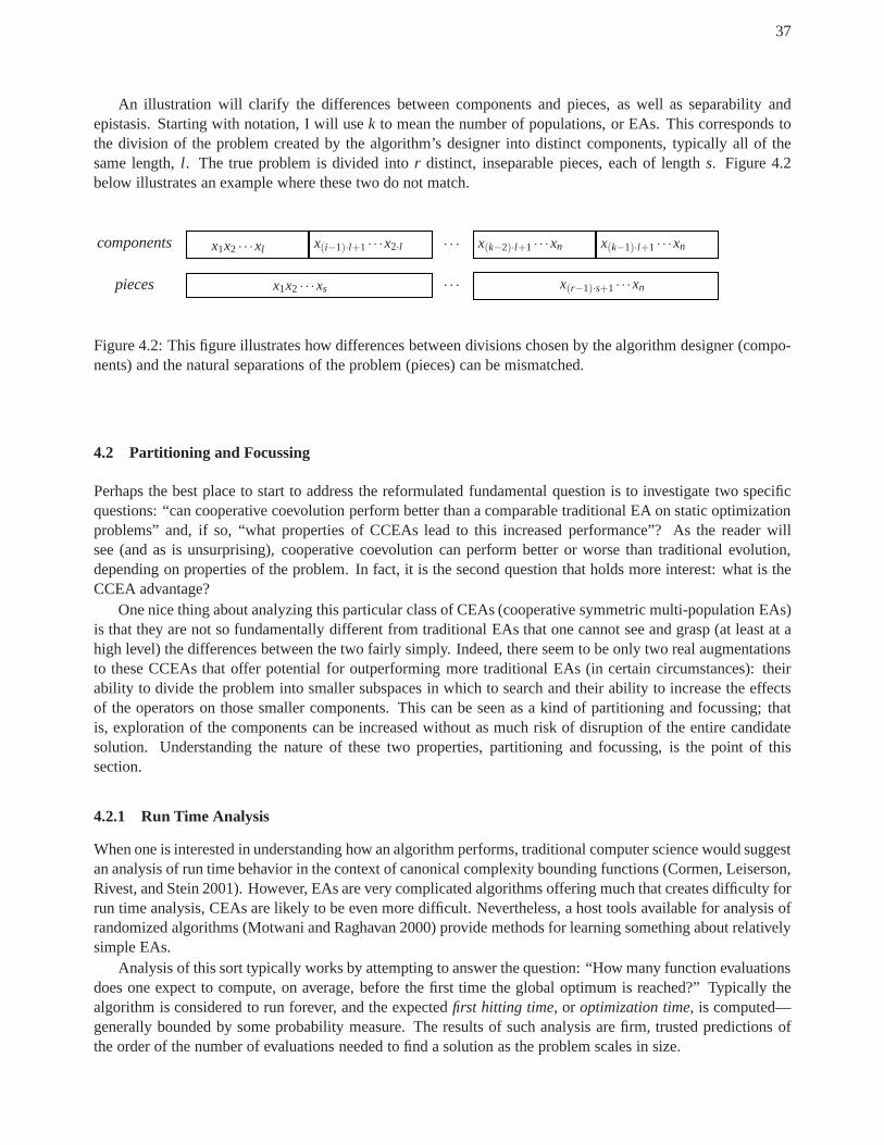
37

An illustration will clarify the differences between components and pieces, as well as separability andepistasis. Starting with notation, I will usek to mean the number of populations, or EAs. This corresponds tothe division of the problem created by the algorithm’s designer into distinct components, typically all of thesame length,l . The true problem is divided intor distinct, inseparable pieces, each of lengths. Figure 4.2below illustrates an example where these two do not match.

components x1x2 · · ·xl x(i−1)·l+1 · · ·x2·l · · · x(k−2)·l+1 · · ·xn x(k−1)·l+1 · · ·xn

pieces x1x2 · · ·xs · · · x(r−1)·s+1 · · ·xn

Figure 4.2: This figure illustrates how differences betweendivisions chosen by the algorithm designer (compo-nents) and the natural separations of the problem (pieces) can be mismatched.

4.2 Partitioning and Focussing

Perhaps the best place to start to address the reformulated fundamental question is to investigate two specificquestions: “can cooperative coevolution perform better than a comparable traditional EA on static optimizationproblems” and, if so, “what properties of CCEAs lead to this increased performance”? As the reader willsee (and as is unsurprising), cooperative coevolution can perform better or worse than traditional evolution,depending on properties of the problem. In fact, it is the second question that holds more interest: what is theCCEA advantage?

One nice thing about analyzing this particular class of CEAs(cooperative symmetric multi-population EAs)is that they are not so fundamentally different from traditional EAs that one cannot see and grasp (at least at ahigh level) the differences between the two fairly simply. Indeed, there seem to be only two real augmentationsto these CCEAs that offer potential for outperforming more traditional EAs (in certain circumstances): theirability to divide the problem into smaller subspaces in which to search and their ability to increase the effectsof the operators on those smaller components. This can be seen as a kind of partitioning and focussing; thatis, exploration of the components can be increased without as much risk of disruption of the entire candidatesolution. Understanding the nature of these two properties, partitioning and focussing, is the point of thissection.

4.2.1 Run Time Analysis

When one is interested in understanding how an algorithm performs, traditional computer science would suggestan analysis of run time behavior in the context of canonical complexity bounding functions (Cormen, Leiserson,Rivest, and Stein 2001). However, EAs are very complicated algorithms offering much that creates difficulty forrun time analysis, CEAs are likely to be even more difficult. Nevertheless, a host tools available for analysis ofrandomized algorithms (Motwani and Raghavan 2000) providemethods for learning something about relativelysimple EAs.

Analysis of this sort typically works by attempting to answer the question: “How many function evaluationsdoes one expect to compute, on average, before the first time the global optimum is reached?” Typically thealgorithm is considered to run forever, and the expectedfirst hitting time, or optimization time, is computed—generally bounded by some probability measure. The resultsof such analysis are firm, trusted predictions ofthe order of the number of evaluations needed to find a solution as the problem scales in size.

38

This analysis provides a good place to start in terms of understanding wider classes of more complicatedEAs. This subsection discusses some early analysis of a simple CCEA, indicating how and when the partition-ing and focussing can give the CCEA an advantage. The majority of the formal analysis in this subsection wasperformed in collaboration with Thomas Jansen during a visit to Dortmund University. This visit was fundedby the Deutsche Forschungsegemeinschaft as a part of the Collaborative Research Center “Computational In-telligence” (SFB 531), and much of the results of this work can be found in Jansen and Wiegand (2003b) and(Jansen and Wiegand 2003c).

The simple CCEA I will analyze here is formulated by using a known simple EA in the Potter frameworkdescribed in the previous chapter.

The (1+1) EA

I begin by describing the simple, analytically tractable (1+1) EA, shown in Algorithm 3 below. Analysis ofthe (1+1) EA has provided the EC community with many results (Muehlenbein 1992; Rudolph 1997; Garnier,Kallel, and Schoenauer 1999; Droste, Jansen, and Wegener 2002; Scharnow, Tinnefeld, and Wegener 2002),as well as tools and methods that could prove useful for analyzing more complicated EAs (Wegener 2002).This simple EA serves the purposes of analysis well, since itis very simple but still quite similar to manymore complicated EAs in many ways. What follows is a formal definition of the (1+1) EA as applied to themaximization of pseudo-Boolean functions. The reader should note that this is a specific case of Algorithm 1.

Algorithm 3 (1+1 Evolutionary Algorithm ((1+1) EA)).

1. Initialize populationChoose x0 ∈ 0,1n uniformly at random.

2. Evaluatepopulationfp = f (x0)

3. t := 04. do

4.1 Select parentsfrom populationUse xt as parent

4.2 Generate offspringfrom parentsCreate y∈ 0,1n by copying xt and, independently for each bit,flip this bit with probabilitymin1/n,1/2.

4.3 Evaluateoffspringfc = f (y)

4.4 Select survivorsfor new populationIf fc ≥ fp, then set xt+1 := y, else set xt+1 := xt .

4.5 t := t + 1until Terminating criteria is met.

This algorithm can be described very simply. There is only one individual in the parent population. Theoffspring is generated by bit-flip mutation on the parent at arate of 1/n, though the mutation probability cannotexceed 1/2. The offspring and parent compete for survival for the next generation, and the offspring survives ifit is as least as good as the parent. It is, as I have said, a simple algorithm about which much is known in termsof run time performance. For example, for all linear functions with non-zero weights (such as ONEMAX ), therunning time is known to beΘ(nlnn); the running time for the LEADINGONES problem is known to beΘ(n2)(Droste, Jansen, and Wegener 2002).

39

The CC (1+1) EA

A simple CCEA can be produced by using the EA defined above in the Potter framework. Such an algorithmhas many benefits for the purposes of analysis. For one thing,it is perhaps the simplest conceivable cooperativecoevolutionary algorithm that can be applied to static optimization problems. This is an attractive propertysince, like the (1+1) EA, it shares some useful properties with more complicated CCEAs, while being analyt-ically tractable. Another useful feature of this simplifiedalgorithm is that the issue of how collaborators areselected is eschewed since the population size for each EA isonly one, by definition. For pedantism, the CC(1+1) EA is described formally, in detail below in Algorithm4. This is an augmentation of Algorithm 2 below.

Algorithm 4 (Sequential Cooperative Coevolutionary 1+1 EA(CC (1+1) EA)).1. for a := 1. . .k

1.1 Initialize population a

Choose x(a)0 ∈ 0,1l uniformly at random.

2. for a := 1. . .k2.1 Evaluatepopulation a

Not applicable3. t := 04. do

4.1 for a:= 1. . .k4.1.1 Select parentsfrom population a

Use x(a)t as parent

4.1.2 Generate offspringfrom parents

Create y(a) ∈ 0,1l by copying x(a)t and, independently for each bit,

flip this bit with probabilitymin1/l ,1/2.4.1.3 Select collaboratorsfrom population

Use all current components of xt , except x(a)t

4.1.4 Evaluateoffspring with collaborators

f (a)c = f

(

x(1)t+1 · · ·y(a) · · ·x(k)

t

)

f (a)p = f

(

x(1)t+1 · · ·x

(a)t · · ·x(k)

t

)

4.1.5 Select survivorsfor new population a

if(

f (a)c ≥ f (a)

p

)

set x(a)t+1 := y(a)

else set x(a)t+1 := x(a)

t

4.1.6 t := t + 1until Terminating criteria is met.

There is only one parent component for each of thek populations. The algorithm works by sequentiallymoving from one population to the next, producing a mutated offspring component, and comparing it againstthe parent in the current context of all other components. Ifthe offspring is at least as good as the parent, theoffspring replaces the parent. It should be noted that this formulation of the CC (1+1) EA requires two evalua-tions for each generation (the parent must be evaluated for each new offspring component, since collaboratingindividuals may have changed from the previous round). Since this results in merely a constant factor in theanalysis, this fact is ignored in this section.

Even at this simple level, there are a variety of choices thatmight have been made yielding slightly differentalgorithms. Predominantly these have to do with which generation provides information to the next. Thedifferences between such “update mechanisms” is explored in more detail in the study presented by Jansenand Wiegand (2003c). In this work, the update mechanism is assumed to work as described above: each EA

40

completes a generation with its respective population before the CCEA moves sequentially to the EA operatingon the next component.

Comparing The (1+1) EA and The CC (1+1) EA (Separability)

Let us suppose for the sake of argument that the CCEA gains itsadvantage chiefly (if not exclusively) fromthe advantage of slicing the problem up and solving the pieces in parallel. This certainly seems to satiate themost straightforward intuition: if the subproblems are linearly independent, surely an algorithm that solvesthese independent subproblems independently in parallel has advantage over the algorithm that treats it as onebig problem? After all, their relative search spaces would (presumably) be much smaller. As a vague sort ofjustification of this intuition, consider a two dimensionaloptimization problemf (x,y) = g1(x)+ g2(y), wherex ∈ a,b,c and y ∈ d,e, f. The algorithm that solves the fullf (x,y) must search a space with 9 searchpoints, while splitting the problem up into two algorithms,each searchingg1(x) andg2(y) respectively onlyneed search three points each, or a total of 6 search points. As the size of the relative sets increases, this gapwidens, of course.

But this is not the space that a CCEA searches, even under the most ideal circumstances, and this notionof subproblems that are separable across population boundaries (even if the design engineer “conveniently” isaware of such divisions in the problem) is also not the advantage it appears to be. To get a better understandingof this it is necessary to first contradict intuition by analyzing the most separable problems conceivable: LINEAR

problems. If the mere splitting of the problem into appropriate partitions is sufficient to gain advantage, onewould expect the biggest advantage to appear when the problem is most divisible. In fact, this is not the case. AsJansen and Wiegand (2003b) shows, the CC (1+1) EA is still bounded above byO(nlnn), yielding no advantagewhatsoever. In fact, it is clear from the analysis produced in that work that no division of the problem will resultin an improvement for the CC (1+1) EA over the simple (1+1) EA.

Why is this? Consider that a linear problem still requires nomore than one-bit mutations for there to beimprovements. Such being the case, the increased focus of attention by the mutation operator offered by theCCEA is not necessary, and cannot be leveraged over the traditional EA for such problems. In fact, for theCC (1+1) EA to show an advantage over the (1+1) EA, the problemmust requireboth the partitioningand theincreased focus of the operators. It must use the partitioning toprotectthe other pieces of the problem from theadded disruption of the more attentive genetic operator. This is not the case in the linear problem.

A problem can be constructed to exhibit this property very clearly. Taking the LOBb problem describedabove, and creating a problem that is separable across population boundaries by “concatenating” several ofthem together in a linear manner, it is easy to construct a problem that has exactly the property in which I aminterested. Allowing, for the moment, the algorithm decomposition to exactly match this new problem’s trueseparability, I can define the new function CLOBb,k in terms of thek populations in the CC (1+1) EA.

Definition 15. For n∈ N, k∈ 1, . . . ,k with n/k∈ N, and b∈ 1, . . . ,n/k with n/(bk) ∈ N, the functionCLOBb,k : 0,1n → R is defined by

CLOBb,k(x) :=

(

k∑

h=1

n·LOBb(

x(h−1)l+1 · · ·xhl)

)

−ONEMAX (x)

for all x = x1 · · ·xn ∈ 0,1n, with l := n/k.

Analysis of both algorithms on this problem shows a clear separation between the CC (1+1) EA andthe (1+1) EA, in terms ofb and k. The expected optimization time of the CC (1+1) EA on the functionCLOBb,k is Θ

(

klb(

lb + lnk

))

with l = n/k, if the CC (1+1) EA exactly matches the function’s separabilitywith k (1+1) EAs, and 2≤ b≤ n/k, 1≤ k≤ n/4, andn/(bk) ∈ N hold. The same problem requires the (1+1)EA Θ

(

nb (n/(bk)+ lnk))

evaluations. Dividing the former by the latter, the difference is obtained and shownbelow.

41

Θ(

nb ·(

nbk + lnk

))

Θ(

klb(

lb + lnk

)) = Θ(

kb−1)

It is interesting to note that for some values ofk andb this can decrease the expected optimization timefrom super-polynomial for the (1+1) EA to polynomial for theCC (1+1) EA. This is, for example, the case fork = n(log logn)/(2logn) andb = (logn)/ log logn. The proofs for these assertions are demonstrated in detailin Jansen and Wiegand (2003b).

Comparing The (1+1) EA and The CC (1+1) EA (Inseparability)

Perhaps the reader is willing to accept that separation may be insufficientto guarantee that a CCEA will outper-form an EA, but thatinseparabilityconstitutes a particular stumbling block for the algorithm. In fact this, too,need not be the case. This is clear when one considers the LEADINGONES problem. Simple analysis can showthat this problem is still solved in quadratic time by both coevolutionary and non-coevolutionary variants of the(1+1) algorithms described above. Though the proof of this (shown below) is a bit tedious, it is nonethelessconstructive and I will include it here for completeness.

Theorem 1. The expected optimization time for the CC (1+1) EA on the function LEADINGONES is Θ(n2).

Proof. The proof for the upper bound is very straightforward. Let uspessimistically assume that the algorithmsolves its components from left to right, one at a time. Droste, Jansen, and Wegener (2002) tells us that theexpected number of active steps needed for a given componentof length l to reach the all-onrd string can bebounded above by 2el2. Since a component is active everyk steps, it will require a given component at most2el2k steps to reach 1l . Components are solved one at a time, so the sum of the expectations can be used to findthe expected waiting time for the entire process,

∑ki=1 2el2k = O(n2). For the lower bound, begin by defining

the termprogressive componentto mean the left-most component that is not the all one string. Note that all ofthe components to the right of the progressive component evolve without influencing the function value. Sincethe original string is drawn at random, and the mutation events are generated independently and uniformly atrandom, the result for each of these components to the right of the progressive component must contain randomstrings. Thus, the process can be treated as successive solutions to individual leading ones problems for eachcomponent. The lower bound for a given component can be obtained from Droste, Jansen, and Wegener (2002),except that now one must show that no advantage can be obtained from the partition.

First, a proof the lower bound for the casel > 3 must be provided. I define the termhead start bitstobe the number of bits that lead a component when that component first becomes the progressive component.Since the string is random until the component becomes progressive, the expected number of such bits canbe bound above byl/3. Chernoff bounds indicates that the probability that there are more than23 l head start

bits is bounded above by34l/3

. Thus, from Droste, Jansen, and Wegener (2002) and this, thelower boundof the expected number of active steps isΩ(l − 2

3 l)2) = Ω(l2/9). A step is active everyk generations, thereareΩ(kl2/9) such generations. The algorithm can be slowed down by assuming that after reaching 1l in theprogressive component, there are no more mutations in the current round. Since each component becomes allone only once, this slows down the optimization by less thank2. Now, in each round at most one componentcan be solved, which yields

∑ki=1 kl2/9 = n2/9 as lower bound. Altogether this yieldsn2/9− k2 = Ω(n2) for

l > 3.For l ≤ 3 it suffices to see that the expected number of leading ones gained in one round is constant. This

implies that there are on averageΩ(k) = Ω(n) rounds before the optimum is reached. In each round there areΩ(n) function evaluations.

42

Of course, the LEADINGONES problem is quite simple; however, itis fully inseparable, meaning it cannotbe partitioned into any linearly independent pieces. Yet inspite of this, as can be seen above, there is noadvantage to the traditional EA over the CCEA: in both cases the expected waiting time for the global optimumis quadratic. The algorithm’s performance seems to be unaffected by the inseparability of the problem. Theproof helps give us insight into at least two of the reasons for this. First of all, this problem must be solved ina specific order in terms of the bit positions in the string, regardless of which algorithm it uses. As a result, thepartitioning makes very little difference to the problem’ssolution, one way or the other. Second, there is nothingintrinsically contradictory in the interrelated bits. TheLEADINGONES function cannot drive the algorithm toa point where its partitioning makes it impossible to make the necessary jump to the solution. This notion of acertainqualityor characteristic propertyof the cross-population epistatic linkages will become more importanta little later in this chapter.

Not only is it the case that inseparability can posenoproblem for the CCEA over the EA, it is not difficult toconstruct problems in which the advantage of the CCEA is preserved, despite the presence of cross-populationepistasis. Moreover, such a problem can exhibit an exponential improvement of the CC (1+1) EA over themore traditional (1+1) EA. The reader is referred to Jansen and Wiegand (2003a) for more details; however,this result should not be surprising, given theNo Free Lunch Theorem(Schumacher, Vose, and Whitley 2001;Wolpert and Macready 1997).

4.2.2 Empirical Analysis

Though asymptotic analysis provides exact answers to questions about the expected waiting time until theglobal optimum is reached, it does have its limitations. Forone, there is a difference between an asymptoticresult and the realistic conditions under which it can be observed. For another, the algorithms analyzed herewere intentionally very simple, and it would be nice to know how the results carry over to somewhat morecomplicated algorithms that are more likely to be used by practitioners.

In fact, in this case the results discussed above hold for both realistic conditions of the (1+1) algorithms, aswell as for somewhat more complicated and realistic algorithms. I will address both of these issue empiricallybelow by considering their behaviors on the CLOBb,k and LEADINGONES problems.

Realistic Problem Conditions

With respect to the first point, knowing that there is an asymptotic difference between the (1+1) EA and the CC(1+1) EA on the CLOBb,k problem (as an example) doesn’t tell uswhenthat difference may become visible.If the constant factors are such that the coevolutionary advantage cannot be seen untiln≥ 1,000,000, then theanalysis may mean very little to people who are applying these methods to real problems. This is not the casethough, as we will shortly see. The CC (1+1) EA advantage overthe (1+1) EA is visible with very reasonablesizes of problem dimensionality.

I performed the following experiments, first on the CLOB2,4 problem, then on the LEADINGONESproblem.A single (1+1) EA and a CC (1+1) EA withk= 4 populations were compared. The algorithms were run in eachcase until the global optimum was found, and the number of function evaluations necessary to achieve this wastracked and reported.

In the case of the CLOB2,4 problem, the algorithm’s representational decompositionmatched the problem’sdecomposition. Thus, there werek = 4 components ands= 4 pieces; however, the size of the components wasvaried, l = 2,4,6,8,10,12,14,16 (n = 8,16,24,32,40,48,56,64). In the LEADINGONES problem thesame(n= 8,16,24,32,40,48,56,64) values were used. This yielded at total of 32 experimental groups (8 for eachproblem, for each group). All groups were run for 50 independent trials.

The results of the CLOB2,4 experiments are not surprising. Figure 4.2.2 on page 44 shows that the CC(1+1) EA performs increasingly fewer evaluations to reach the global peak than its EA counterpart. This

43

difference is statistically significant forl ≥ 2 at a 95% confidence usingt-tests and the Bonferoni adjustment(Hancock and Klockars 1996). On the other hand, Figure 4.2.2(same page) shows no significant difference(either visually or statistically) between the two algorithms over the same range ofn values. This indirectlyvalidates the theoretical results directly in realistic sizes dimensions of the search space: the coevolutionaryvariant is superior to the traditional variant on the separable CLOB2,4 problem, but they are indistinguishable(in terms of performance) on the inseparable LEADINGONES problem for alln> 8. In both cases a more directvalidation would be achieved by considering the ratio of thecurves and determining whether this ratio wasnon-constant. To do this, experiments with larger values ofn would need to be run.

Realistic Algorithms

One complaint that has been leveled against the analytical work that has focussed on the (1+1) EA (and, byextension, this work focussing on the CC (1+1) EA), is the fact that it does not appear to be a “realistic”algorithm in the sense that it is not one that practitioners are likely to use. While a comprehensive study ofa wide catalog of coevolutionary algorithms is outside the scope and point of this dissertation, there are somenatural steps that can be made to make this algorithm a bit more realistic. Here I describe one such step andconduct the same empirical studies as were presented above on these more plausibly practical EAs.

The non-coevolutionary EA works as follows. There is a population of parents (in this case 10), and at eachstep a single offspring is produced by fitness proportionateselection and bit-flip mutation, with a probability of1/n, wheren is the length of the bit string. The offspring is then evaluated and compared with parent population,replacing the worst member if it is at least as good. If there are more than one such parents, then one is selectedat random for deletion. This is the so-calledsteady stateEA (De Jong 1975). The reader should be carefulto note that this algorithm is not too terribly different than the (1+1) EA. In a sense, one could consider it amodified (µ+1) EA, where proportionate parent selection is used ratherthan uniform random selection. This isan intentional choice, as it lends itself well toward futureexpansions of the theoretical analysis. I will refer tothis as the SS-EA

The coevolutionary variant of this should be of no surprise.In this case, there arek (again herek = 4)populations, each of size 10. As with the sequential CC (1+1)EA, the populations of this SS-CCEA areprocessed sequentially, in order. In each case, one step of the underlying steady state EA is performed. Nowthat there is a population, though, I must address the issue of collaboration. For now, I will simply pick a singleindividual from each of the other populations that has the highest fitness from the last time that population wasprocessed (the so-calledsingle-bestcollaboration strategy).

Again I consider the CLOB2,4 and LEADINGONES problems with the same experimental groups:l =2,4,6,8,10,12,14,16 for CLOB2,4 andn = 8,16,24,32,40,48,56,64 for LEADINGONES. Again all 32groups were for 50 independent trials.

The results of the CLOB2,4 experiments are consistent with those of the simpler (1+1) variants. Figure 4.2.2on page 45 shows that the SS-CCEA still statistically significantly outperforms its EA counterpart (95% confi-dence usingt-tests and the Bonferoni adjustment), though for thel ≥ 2 groups now. Additionally, Figure 4.2.2(same page) still shows no significant difference between the two algorithms over the same range ofn values.This justifies, to some extent, the use of the simple algorithm: the theoretical results for the simpler (1+1) al-gorithms seem to hold for similar population-based approaches. Here again the values ofn are too small to seenon-constant ratios between the the curves.

4.2.3 The Parallel CC (1+1) EA

The above analysis reflects consideration of Algorithm 4 described on page 39. As I’ve already mentioned,this algorithm issequentialin the sense the individual components are processed one at atime, in order. Thisallows for changes in an individual occurring during a roundto affect the fitness of individuals representingdifferent components evaluated later that same round. Alternatively, one might apply a moreparallel updating

44

2 4 6 8 10 12 14 16

050

000

1000

00

l

Eva

ls(1+1) EACC (1+1) EA

Figure 4.3: Results for the CC (1+1) EA (black) and the (1+1) EA (dashed, dark grey) on the CLOB2,4 problem.The x-axis shows the length of a component,l , and the they-axis shows the number of function evaluationsuntil the global optimum was reached. The vertical wings show the 95% confidence interval of 50 independenttrials; the plotted point shows the mean.

10 20 30 40 50 60

020

0040

0060

0080

00

n

Eva

ls

(1+1) EACC (1+1) EA

Figure 4.4: Results for the CC (1+1) EA (black) and the (1+1) EA (dashed, dark grey) on the LEADINGONES

problem. Thex-axis shows the length of a component,l , and the they-axis shows the number of functionevaluations until the global optimum was reached. The vertical wings show the 95% confidence interval of 50independent trials; the plotted point shows the mean.

45

2 4 6 8 10 12 14 16

020

000

4000

060

000

8000

0

l

Eva

lsSS−EASS−CCEA

Figure 4.5: Results for the SS-CCEA (black) and the SS-EA (dashed, dark grey) on the CLOB2,4 problem. Thex-axis shows the length of a component /piece,l , and the they-axis shows the number of function evaluationsuntil the global optimum was reached. The vertical wings show the 95% confidence interval of 50 independenttrials; the plotted point shows the mean.

10 20 30 40 50 60

050

010

0015

0020

00

n

Eva

ls

SS−EASS−CCEA

Figure 4.6: Results for the SS-CCEA (black) and the SS-EA (dashed, dark grey) on the LEADINGONES prob-lem. Thex-axis shows the length of a component /piece,l , and the they-axis shows the number of functionevaluations until the global optimum was reached. The vertical wings show the 95% confidence interval of 50independent trials; the plotted point shows the mean.

46

approach, where individuals select collaborators from theprevious round, allowing no inter-round changesto have any affect on the fitness result from individuals evaluated in the current round. I call this parallelbecause the components can then be processed asynchronously in any order, or they can be processed in parallel.Algorithm 5 can be obtained by simply making a slight change in line 4.1.4 of Algorithm 4. This substitutedline is shown below.

Algorithm 5 (Parallel CC (1+1) EA).

4.1.4 Evaluateoffspring with collaborators

f (a)c = f

(

x(1)t · · ·y(a) · · ·x(k)

t

)

f (a)p = f

(

x(1)t · · ·x(a)

t · · ·x(k)t

)

The reader should note that using the previous round’s individuals for the evaluation affects not only theoffspring evaluation, but the parent’s as well. In fact, in the parallel variant one need only evaluate the parentonce a round, since its value will never change while the round is in progress. This gives the parallel imple-mentation an implicit advantage in terms of the number of evaluations performed, albeit by at most the constantfactor 2.

The situations in which these two variants differ are perhaps less than obvious. Let’s first look at the situ-ation where problems are separable across population boundaries, then turn attention to a problem constructedto exploit the difference between these two algorithms. I will return to this algorithm at the end of the chapterto discuss some of its pathologies compared to those of the sequential model.

Equivalence on Separable Functions

Conventional wisdom suggests that, while these two algorithms are very similar, they make a fundamentallydifferent type of choice with respect to selection and updating, and thus can differ profoundly from one another.While this is true in the general case, it is not true for problems in which components relate in merely linearways. Indeed, the parallel and sequential variants of the CC(1+1) EA have equivalent running times on allfunctions that are separable across population boundaries. The proof of this is shown below for Theorem 2.

The result of this is to suggest a far more subtle difference between these two algorithms. Certainly theydiffer, and thus must exhibit different running times for some problems, but not for separable ones. This analysissuggests that if an algorithm designer is confident that their decomposition matches that of the true problem,there is no reason based on running time alone to choose the sequential algorithm over the parallel, or vice-versa. Thus they are free to consider other factors in makingthis decision (such as whether or not a parallelcomputational environment exists of which they can take advantage, for instance).

Theorem 2. For any function f: 0,1n → R, if the parallel and sequential forms of the CC (1+1) EA use thesame division into components on f and if f is separable across population boundaries, then the twoCC (1+1) EAs behave identically.

Proof. Contradiction is used to show that the two algorithms must have the same performance because theybehave identically in all cases when applied to the same separable problem. Given that they behave identically,the number of generations needed for optimization is equivalent, and their respective expected waiting timesfor the global optimum cannot differ by more than a factor of two.

For there to be any difference in behaviors, the algorithms must make different decisions during the selectionstep, and by consequence the evaluation step, step 4.1.4, must obtain different results. Given that the functionis separable across population boundaries, the linear contribution of the active component to the total fitness,ga : 0,1l → R, can be the only difference in the total fitness score. As a result, for a different selection

decision to be made, it must be true thatga(y(a)) ≥ ga(x(a)t ) andga(y(a)) < ga(x

(a)t ). Since both inequalities

cannot be simultaneously true, there is a contradiction.

47

Tricking The Sequential (or Parallel) Algorithm

Despite the fact that the parallel and sequential CC (1+1) EAs are very similar algorithms, and despite the factthat they perform identically on problems that are separable across population boundaries, they are neverthelessdifferent algorithms and behave differently on some problems. The problem classes for which a distinction inrunning time is possible are a subset of problems containingcross-population epistatic linkages; however, thereis no reason to believe that all such problems pose an advantage to one or the other—quite the reverse: someproblems favor sequential algorithms and some favor parallel algorithms. Let’s begin by looking at the latter.

When might a parallel algorithm gain advantage over the sequential algorithm? To see this, first note thatthe parallel algorithm actuallythrows information awayin the sense that information might be learned duringa round, but cannot be used until the next round, after other changes may have occurred. It makes sense, then,that parallel algorithms are favored when such informationis misleading in some way. With a bit of effort, sucha situation can be constructed. Consider the definitions below.

Definition 16. For any m∈ N with m≥ 6, we define n:= 2m and the function g: 0,1n → R. Forx = x1 · · ·xn ∈ 0,1n the x string can be written x= x′x′′ with x′ = x1 · · ·xm ∈ 0,1m andx′′ = xm+1 · · ·xn ∈ 0,1m. The function g is defined by

g(x) :=

2n+2 if x = 0n

2n+n· ‖x‖ if x′ = 0m ∨ x′ = 0m

2n+1 if x′ 6= 0m ∧ x′′ 6= 0m ∧ ‖x‖ = 2

2n+2· ‖x‖ if x′ 6= 0m ∧ x′′ 6= 0m ∧ ‖x‖ > 2 ∧(‖x′‖ < ⌈m/3⌉ ∨ ‖x′′‖ < ⌈m/3⌉)

n4 +‖x‖ otherwise

for all x ∈ 0,1n, where‖x‖ = ONEMAX (x).

This function,g: 0,1n →R, is not(r,s)-separable for anys< n. What is of interest is the performance ofthe two CC (1+1) EA variants ong when using two sub-populations, one operating onx′ and the other operatingon x′′. These two parts are non-linearly related, but splitting them up in this way will facilitate opportunitiesfor the parallel and sequential algorithms to come to different conclusions based on the information they haveat their disposal when processing a given generation. One more layer is needed to complete this picture: let’sembedg into another function, SEPFUN, the target of our analysis. Now the difference between these twovariants is clear and provable.

Definition 17. For any k∈ N with k≥ 6, define n:= 4k2, m:= n/2 = 2k2 and the functionSEPFUN : 0,1n → R. For x= x1 · · ·xn ∈ 0,1, the x string can be written x= x′x′′ withx′ = x1 · · ·xm ∈ 0,1m and x′′ = xm+1 · · ·xn ∈ 0,1m. For x′ = x1 · · ·xm ∈ 0,1m, the x′ substring can bewritten x′ = x(1)x(2) · · ·x(k) with x(i) = x2(i−1)k+1 · · ·x2ik for all i ∈ 1, . . . ,k. The functionSEPFUN is definedby

SEPFUN(x) :=

n−‖x′‖+ LEADINGONES(x′′) if x′′ 6= 1m

n+k∑

i=1g(

x(i))

otherwise


As I will discuss at the end of this chapter, neither the sequential nor the parallel algorithm are able to findthe global max for some types of problems with cross-population epistasis. This is such a problem: there is noexpectation that the CC (1+1) EA finds the global optimum of SEPFUN. Instead one must change perspectiveto one of approximation. I wish to know which of the two algorithms finds the larger function value in a specificnumber of generations, fixed in advance. Concentrating on a large but still polynomial numbers of generations,

48

Jansen and Wiegand (2003c) prove that for the sequential algorithm, the best fitness is so-far discovered intsteps (wheret ≥ 6n5/2 +6n2 andt = nO(1)) is n2

4 +n3/2+n with overwhelming probability. In the same numberof steps, the parallel variant will have attained then4 case fromg. Jansen and Wiegand (2003c) verify thisexperimentally, as well.

Perhaps more interesting than this, however, is the fact that a relatively obvious change in the underlyingfunction reverses the situation. Consider an alternativeg′ below, substituted in SEPFUN for g.

Definition 18. For any m∈ N with m≥ 6, we define n:= 2m and the function g′ : 0,1n → R.For x = x1 · · ·xn ∈ 0,1n, the x string can be written x= x′x′′ with x′ = x1 · · ·xm ∈ 0,1m andx′′ = xm+1 · · ·xn ∈ 0,1m. The function g′ is defined by

g′(x) :=

2n+2 if x = 0n

2n+n‖x‖ if x′ = 0m∨x′′ = 0m

2n+1 if x′ 6= 0m∧x′′ 6= 0m∧‖x‖ = 2

2n+2‖x‖ if x′ 6= 0m∧x′′ 6= 0m∧‖x‖ > 2

n4 +‖x‖ otherwise


Now the sequential implementation is clearly superior, because havingx(i) ∈

1k0k,0k1k

yields much better pay-off thanx(i) = 12k. Thus, while in some cases the parallel variantclearly performs better than the sequential algorithm, in other cases the reverse is true. The basic advantage ofthe parallel over the sequential CC (1+1) EA seems to center around whether accrual of local information duringa round will be misleading, while this advantage is reversedif the omission of such information is misleading.Again there is no general reason (without domain knowledge)to apply one or the other type of algorithm.

4.3 Collaboration

Selecting a collaboration method for a CCEA is one of the mostimportant decisions an engineer must make.Not only can such methods make or break the performance of real CCEAs on real problems, the availablechoices seem to be integrally tied to certain problem properties. Many researchers believe that the existenceof cross-population epistasis will demand more sophisticated collaboration methods. This section presentsempirical analysis of the collaboration mechanism from theperspective of this property.

4.3.1 Sampling Interactions

Independent EAs in a coevolutionary framework operates on components with incomplete information. Recallthe thought exercise earlier where the search space seems tobe reduced by splitting the problem into twoparallel and independent searches of the linearly separable pieces of the problem. This idea is flawed becausethe coevolutionary algorithm isnot only searching the projection of the problem. It is searching a projection ofthe problemat one time, and this projectionchangesthroughout time, as the other populations change.

Collaboration is the process by which the population currently under evaluation collects information andthe whole problem, about the relationship between components. Despite the fact that CCEAs will look only ata projection of the problem at any one time, the quality of that projection in terms of their ability to characterizethe relevant features of the complete search space depends largely on the tractability of that characterization, aswell as the ability of the collaboration process to gather useful information about the other populations.

The best way to think about the collaboration process is to consider it as a method forsampling interactionspace. Given this view, how one selects collaborators is a major issue since the degree of complexity of theinteraction space is complicated. It may be that more collaborators are needed per evaluation in order to better

49

characterize the interaction space (a larger sample size),or that theway they are picked might lead to moreefficient use of the samples one already has (a biased sample), etc. If one selects more collaborators than isnecessary, search performance is harmed by unnecessary evaluations. In the worst case, complete mixing isused. In complete mixing all individuals are coupled with all individuals from all populations. This becomescombinatorially large as the number of populations increase linearly. However, if only a single individualfrom each population is sampled for collaboration, the algorithm may have insufficient information about theinteraction space with which to construct a suitable searchgradient. This problem is worse when such anindividual is chosen poorly. The questions is: What kinds ofsampling methods are most appropriate forproblems with different properties?

4.3.2 Decompositional Bias

As we have already seen, different problems have different degrees of separability that may or may not corre-spond with particular CCEA representation choices. Since separability information is not generally availablefor difficult optimization problems, the focus here is on thecase where there is a particular kind of mismatchbetween the CCEA representation and a problem’s “natural” decomposition. The issue here is not whether suchmismatches make the problem harder to solve. This will clearly happen for some problems (Potter and De Jong1994; Bull 1997; Bull 2001; Wiegand, Liles, and De Jong 2001). Instead, the question is whether adoptingmore complex collaboration methods can alleviate such mismatches.

In order to answer this, it is useful to have problems that canbe explicitly controlled in terms of theirinherent separability. For pseudo-boolean functions thisis not difficult using the method of concatenationalready mentioned. From a practitioner’s point of view, barring any problem specific domain knowledge, thesimplest way to represent pseudo-boolean functions is to again break up the total bit string of lengthn into kequal sized components of lengthl and assign each component to a different population. Recallthat r denotesthe number of separable pieces of lengths. Given these two different divisions, a decompositional mismatchof the representation may be due toover-decomposition(k > r) or under-decomposition(k < r). If there aremore populations than there are separate pieces of the problem, there is likely to be strong interaction betweenpopulations in the system with respect to the problem, i.e.,cross-population epistasis. Ifk < r, the advantageof the parallelism of coevolutionary search is sacrificed.

Again, our interest is whether difficulties due to the existence of decompositional bias can be alleviated bymore complex collaboration methods. The motivation for this interest stems from an important observation: ifthere is no cross-population epistasis, a simple selectionmethod for collaboration is sufficient. If two popula-tions represent independent pieces of the problem, then optimizing one population independently of the otherwill result in the complete optimization of the problem. As long as the collaborator chosen for each populationmember is the same, it doesn’t matter how one chooses it. However, it does matter how many collaboratorsone chooses, since picking more than one will incur more unnecessary evaluations. Therefore, in the absenceof cross-population epistasis, selecting the single best individual (i.e., the most fit individual(s) in other popu-lation(s) from previous evaluation) from the other populations for collaboration is sufficient. In fact, one couldpick this individual randomly, as long as it was the same individual for each member of the population duringa given generation. The point isn’t that any partnering scheme will result in a better collaboration than another,but that since each population can essentially be optimizedindependently, one only needs aconsistentsamplefrom which to establish collaboration.

So when would a more complicated collaboration selection method be needed? Recall that how one choosescollaborators essentially determines how onesamples the potential interactionswith the other population. Therehas to be a reason to believe that more than one sample is needed, or that sampling with a particular bias(say choosing the best) will result in a qualitatively different characterization of the relationship between thepopulations. Either way, some interaction between the populations is certainly needed to justify this need. Morethan simply having such epistasis is at issue, however.

In order to study the effects of collaboration on such situations, the following experiment was constructed.

50

The steady state CCEA (SS-CCEA) described above was appliedto a concatenated LEADINGONES problem.In this particular case there were 128 bits in the total bit string of the problem, subdivided evenly intor = 2pieces. The function below gives a more specific descriptionof this function.

f (x) = LEADINGONES(

x(1))

+ LEADINGONES(

x(2))

A total of 6 collaboration selection methods were used. The number of collaborators chosen for a givenevaluation was varied (1,2,&3) and two selection biases were used:c-best andc-random. These worked asfollows. In the first case, thec best individuals were chosen from each of the other populations, evaluatedwith the current individual, and the best of those scores wasused as the fitness value for the individual. In thesecond case,c individuals were chosen uniformly at random without replacement, evaluated with the currentindividual, and again the best of those scores were used as the fitness value for the individual.

Aside from these 6 collaboration methods, the number of populations,k, was varied. However, in all casesthe number of individuals in each population was 10. The results for k = 2 throughk = 16 in Table 4.1 showthe average number of evaluations for the algorithms to reach the optimum. There were 50 trials performed pergroup. Unless otherwise stated, confidence levels for all tests are 95%.

Table 4.1: Steady state CCEA results on the LEADINGONES problem. Each value represents the mean numberof evaluations needed to reach the optimum out of 50 trials. From the top left corner, proceeding clockwise, thetables represent data for decompositional biases created using two, four, eight and sixteen populations.

r = k # Collaborators1 2 3

c-best 8841.56 17546.52 25331.32c-rand 8838.46 17621.88 25640.28

k = 4 # Collaborators1 2 3

c-best 9355.16 18994.36 28061.20c-rand 10636.90 19229.02 28769.28


c-best 10420.48 21178.52 31253.44c-rand 13161.24 23657.76 34302.52


c-best 11930.08 23723.20 34587.76c-rand 19458.44 30713.74 42862.28

Statistically, the relevant groups were compared with at-test using the Bonferoni adjustment. In all caseschoosing one collaborator is significantly better. This might at first be puzzling since there is clearly cross-population epistasis present whenk > 2. However, note that a mutation that turns some bit to 1 in an individualin the first population will always result either a neutral orpositive change in fitness, regardless of the contentsof the other population. The reverse is also true. In addition, this fact is not true symmetrically fork = 4. Thesecond and fourth populations will remain relatively unimportant to the first and third populations for sometime during the evolution, since each LEADINGONES subproblem is solved left-to-right. This is essentially thesame observation made by the formal analysis of the CC (1+1) EA, above.

Observe that by changing the number of populations, the mutation rate is effectively being increased (recallthat the mutation is 1/l , wherel is the number of bits per individual in each population). Such issues may affectthe empirical results, consequently I ran all population-oriented experiments discussed above with a constant1/64 mutation rate. The results (below) remain consistent with those reported above. Again, statisticallyspeaking it is better to select only a single collaborator.

Recall that one observation about the LEADINGONES problem made during formal analysis earlier in thischapter was that there is nothing intrinsically contradictory in the interrelated bits of this problem. This can be

51

Table 4.2: Steady state CCEA results on the LEADINGONES problem with a constant mutation rate of 1/64 forall experimental groups. Each value represents the mean number of evaluations needed to reach the optimumout of 50 trials. From the top left corner, proceeding clockwise, the tables represent data for decompositionalbiases created using two, four, eight and sixteen populations.


c-best 8428.28 17315.64 26535.94c-rand 9103.48 17128.94 26677.74


c-best 12646.04 27122.52 37218.52c-rand 13759.30 27517.72 39194.62


c-best 22654.56 42379.00 68231.68c-rand 24298.46 45986.04 69805.16


c-best 40193.10 79460.12 119571.76c-rand 43751.84 83424.06 124537.00

easily rectified by a simple change to the problem: scale the LEADINGONES part bys and subtract ONEMAX

from the total, i.e.,g(x(i)) = s· LEADINGONES(x(i))−ONEMAX (x(i))+ s, and f (x) =∑k

i=1g(x(i)). The en-tire function is translated up bys to prevent any negative values that will create a difficulty for the fitnessproportionate selection method.

With this new function the right side will affect the search since bits to the right of the left-most zero bitwill contribute to fitness, but there is some tension betweenindividual bit contributions to fitness and those oftheir non-linear interactions since those right-side bitscontributenegatively. This modification is a half-steptowards pure contradiction since this tension is one directional. Take the string: “110000. . .” as an example.Flipping the fourth bit to a one will decrease the fitness slightly if the third bit remains 0, while flipping boththe third and fourth bits will increase the fitness. However,the same is not true on the other side. Flipping thethird bit while the fourth bit remains 0 will also increase fitness. So some of the interactions have this propertyof sign-dependent epistasis, while others will not. In addition, the linear effects of the bits are very mutedcompared to the non-linear effects due to the scaling issue.

Thiss·LEADINGONES−ONEMAX function is again concatenated using two pieces (r = 2), that is f (x) =g(

x(1))

+g(

x(2))

. Again, I applied the SS-CCEA algorithm using the 6 collaboration methods described above.The results fork = 2 throughk = 16 in Table 4.3 show the average number of evaluations it tookthe algorithmsto reach the optimum (50 trials each).

In addition to the data presented, I performed similar experiments at higherk values. In all cases there wasagain no statistical reason to choose another collaboration method other than the single best individual from theother populations. Not only does this increased decompositional bias not alter the collaboration methodology,it appears as though this problem becomeseasier for the CCEA to solve, not harder, when using thec-beststrategies. This turns out to be statistically significant only for the k = 16 andk = 64 cases where using thesingle-best strategy, for thek≥ 16 cases using 2-best, and thek= 32 andk= 64 cases using 3-best. Figure 4.3.2below shows results for thec-best strategies ask is increased in2,4,8,16,32,64.

So far, these experiments confirm what one sees in practice, namely that the simple collaboration methodinvolving just the best individuals from each population isquite robust even when there is cross-populationepistasis. However, what is still not clear is when it fails.To understand that better, I next focus on the thevarious forms of cross-population epistasis.

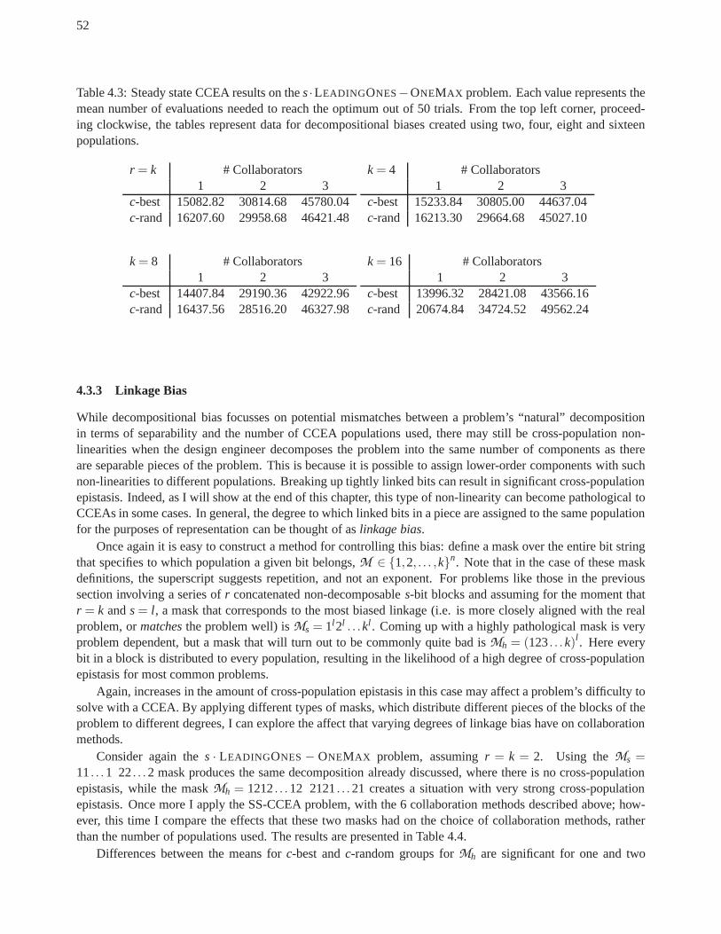
52

Table 4.3: Steady state CCEA results on thes·LEADINGONES−ONEMAX problem. Each value represents themean number of evaluations needed to reach the optimum out of50 trials. From the top left corner, proceed-ing clockwise, the tables represent data for decompositional biases created using two, four, eight and sixteenpopulations.


c-best 15082.82 30814.68 45780.04c-rand 16207.60 29958.68 46421.48


c-best 15233.84 30805.00 44637.04c-rand 16213.30 29664.68 45027.10


c-best 14407.84 29190.36 42922.96c-rand 16437.56 28516.20 46327.98


c-best 13996.32 28421.08 43566.16c-rand 20674.84 34724.52 49562.24

4.3.3 Linkage Bias

While decompositional bias focusses on potential mismatches between a problem’s “natural” decompositionin terms of separability and the number of CCEA populations used, there may still be cross-population non-linearities when the design engineer decomposes the problem into the same number of components as thereare separable pieces of the problem. This is because it is possible to assign lower-order components with suchnon-linearities to different populations. Breaking up tightly linked bits can result in significant cross-populationepistasis. Indeed, as I will show at the end of this chapter, this type of non-linearity can become pathological toCCEAs in some cases. In general, the degree to which linked bits in a piece are assigned to the same populationfor the purposes of representation can be thought of aslinkage bias.

Once again it is easy to construct a method for controlling this bias: define a mask over the entire bit stringthat specifies to which population a given bit belongs,M ∈ 1,2, . . . ,kn. Note that in the case of these maskdefinitions, the superscript suggests repetition, and not an exponent. For problems like those in the previoussection involving a series ofr concatenated non-decomposables-bit blocks and assuming for the moment thatr = k ands= l , a mask that corresponds to the most biased linkage (i.e. is more closely aligned with the realproblem, ormatchesthe problem well) isMs = 1l 2l . . .kl . Coming up with a highly pathological mask is veryproblem dependent, but a mask that will turn out to be commonly quite bad isMh = (123. . .k)l . Here everybit in a block is distributed to every population, resultingin the likelihood of a high degree of cross-populationepistasis for most common problems.

Again, increases in the amount of cross-population epistasis in this case may affect a problem’s difficulty tosolve with a CCEA. By applying different types of masks, which distribute different pieces of the blocks of theproblem to different degrees, I can explore the affect that varying degrees of linkage bias have on collaborationmethods.

Consider again thes · LEADINGONES− ONEMAX problem, assumingr = k = 2. Using theMs =11. . .1 22. . .2 mask produces the same decomposition already discussed, where there is no cross-populationepistasis, while the maskMh = 1212. . .12 2121. . .21 creates a situation with very strong cross-populationepistasis. Once more I apply the SS-CCEA problem, with the 6 collaboration methods described above; how-ever, this time I compare the effects that these two masks hadon the choice of collaboration methods, ratherthan the number of populations used. The results are presented in Table 4.4.

Differences between the means forc-best andc-random groups forMh are significant for one and two

53

0 10 20 30 40 50 60

2000

030

000

4000

0

k

Eva

ls

3−best2−best1−best

Figure 4.7: Results for the SS-CCEA on thes· LEADINGONES−ONEMAX problem for increasing values ofk. The bottom curve (solid) illustrates results for the single-best collaboration strategy, the middle curve (longdashed) represents results for the 2-best, and the top curve(short dashed) represents results for the 3-best. Thex-axis shows the size ofk, and the they-axis shows the number of function evaluations until the global optimumwas reached. The vertical wings show the 95% confidence interval of 50 independent trials; the plotted pointshows the mean.

collaborators, but not for three. There are no statistically significant differences between these groups (for thesame number of collaborators) for the simpler linkage bias.

Once again simply distributing the epistatic linkages across the population boundaries is insufficient torequire that a more complicated collaboration method be used. This may seem surprising at first, but note that,for this particular problem, introducing such masks does not change thetypeof cross-population epistasis, onlyits degree. Moreover, although not germane to our question,it is interesting to note that in this particular caseincreasing the mixing seems toimproveperformance versus theMs mask (this is significant for all but the3-random case).

What remains to be shown is what the effect of the most difficult form of cross-population epistasis has oncollaboration selection. When neither the sign nor the magnitude of the interaction can be reliably predicted,will it become necessary to select collaborators differently? Intuition seems to suggest that it will. If noprediction can be made about the higher order blocks from thelower order blocks, then a more sophisticatedmethod of sampling the interaction space should be needed. What I need to do now is construct a problem withjust such a challenge.

Fortunately, the CLOBb,k problem mentioned previously has exactly this property. Note that this problemis already one constructed by concatenation of functions over smaller, inseparable pieces. Because this problemis already quite difficult whenb= 2 and I am looking at linkage bias, rather than decompositional bias, here thefocus is on the specific function CLOB2,2. This offers the simplest such problem still more complicated thanthes·LEADINGONES−ONEMAX . As it turns out, it is so difficult under theMh mask that the algorithms didnot find the global optimum withn = 128. The reason for this should be clear by the end of this chapter. Atany rate, as a consequence Table 4.5 represents the mean fitness values obtained after a fixed budget of 100,000evaluations. The reader should be careful to note that in this case higher values are better.

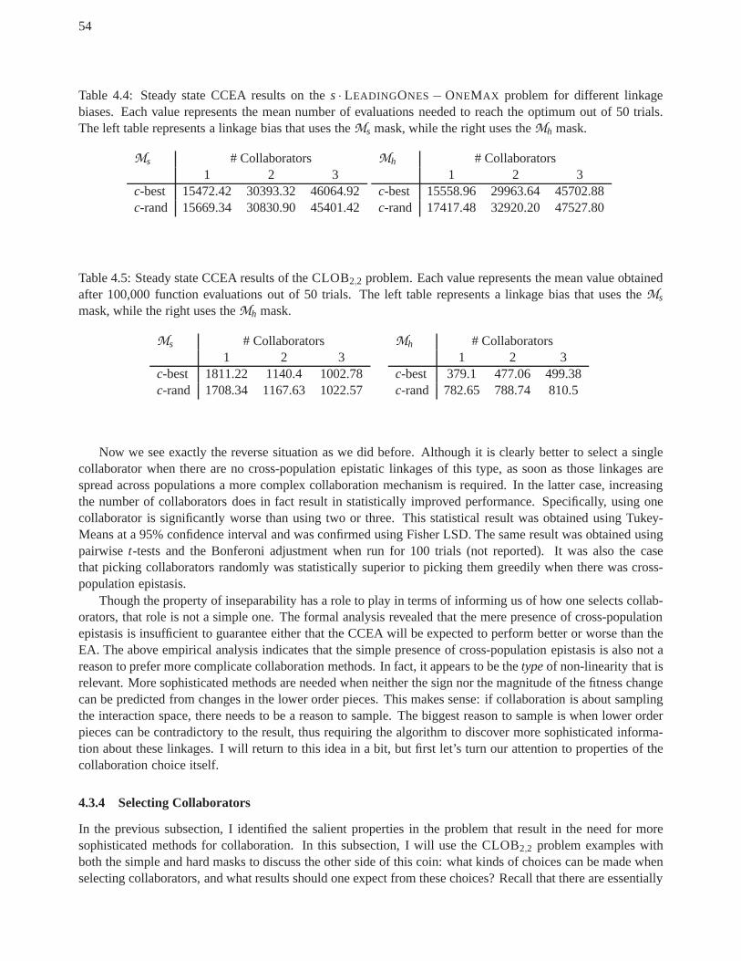
54

Table 4.4: Steady state CCEA results on thes· LEADINGONES− ONEMAX problem for different linkagebiases. Each value represents the mean number of evaluations needed to reach the optimum out of 50 trials.The left table represents a linkage bias that uses theMs mask, while the right uses theMh mask.

Ms # Collaborators1 2 3

c-best 15472.42 30393.32 46064.92c-rand 15669.34 30830.90 45401.42

Mh # Collaborators1 2 3

c-best 15558.96 29963.64 45702.88c-rand 17417.48 32920.20 47527.80

Table 4.5: Steady state CCEA results of the CLOB2,2 problem. Each value represents the mean value obtainedafter 100,000 function evaluations out of 50 trials. The left table represents a linkage bias that uses theMs

mask, while the right uses theMh mask.

Ms # Collaborators1 2 3

c-best 1811.22 1140.4 1002.78c-rand 1708.34 1167.63 1022.57

Mh # Collaborators1 2 3

c-best 379.1 477.06 499.38c-rand 782.65 788.74 810.5

Now we see exactly the reverse situation as we did before. Although it is clearly better to select a singlecollaborator when there are no cross-population epistaticlinkages of this type, as soon as those linkages arespread across populations a more complex collaboration mechanism is required. In the latter case, increasingthe number of collaborators does in fact result in statistically improved performance. Specifically, using onecollaborator is significantly worse than using two or three.This statistical result was obtained using Tukey-Means at a 95% confidence interval and was confirmed using Fisher LSD. The same result was obtained usingpairwise t-tests and the Bonferoni adjustment when run for 100 trials (not reported). It was also the casethat picking collaborators randomly was statistically superior to picking them greedily when there was cross-population epistasis.

Though the property of inseparability has a role to play in terms of informing us of how one selects collab-orators, that role is not a simple one. The formal analysis revealed that the mere presence of cross-populationepistasis is insufficient to guarantee either that the CCEA will be expected to perform better or worse than theEA. The above empirical analysis indicates that the simple presence of cross-population epistasis is also not areason to prefer more complicate collaboration methods. Infact, it appears to be thetypeof non-linearity that isrelevant. More sophisticated methods are needed when neither the sign nor the magnitude of the fitness changecan be predicted from changes in the lower order pieces. Thismakes sense: if collaboration is about samplingthe interaction space, there needs to be a reason to sample. The biggest reason to sample is when lower orderpieces can be contradictory to the result, thus requiring the algorithm to discover more sophisticated informa-tion about these linkages. I will return to this idea in a bit,but first let’s turn our attention to properties of thecollaboration choice itself.

4.3.4 Selecting Collaborators

In the previous subsection, I identified the salient properties in the problem that result in the need for moresophisticated methods for collaboration. In this subsection, I will use the CLOB2,2 problem examples withboth the simple and hard masks to discuss the other side of this coin: what kinds of choices can be made whenselecting collaborators, and what results should one expect from these choices? Recall that there are essentially

55

three attributes to consider for collaborator selection: sample size, selective pressure, and credit assignment.

The first case is simple since the sample size can be controlled simply by controlling the number of col-laborators selected. As above, I will usec to denote the size of the collaborator sample. Of course, thelargerthis value is, the more objective evaluations will be required per individual. It should be clear that increas-ing the sample size and the number of populations together can have a combinatorial effect on these functionevaluations. So, in general, it would seem that the fewer collaboratorswe needto obtain “good” results, thebetter.

The second case requires a slightly more complicated mechanism. In this case, a simple tournament drawmethod can control the degree of selective bias of collaborators. That is, the algorithm selectsq collaborators atrandom with replacement, and chooses the one with the highest fitness from its previous evaluation. This doesnot increase the number of function evaluations performed since the algorithm simply uses the results fromprevious evaluation. The net effect is that the selection pressure can be increased from purely random (q = 1)to elitist (q :≈ plg p, wherep is the population size).

When multiple collaborators are evaluated for the purposesof fitness (whenc > 1), there is still the openquestion of how one assigns a single fitness score from the results of multiple objective function evaluations,collaborator credit assignment. Here only three possible credit assignment methods are considered:optimistic,hedge, andpessimistic. These correspond respectively to using the max, mean, and min of the c availableobjective function results.

Let’s consider collaborator credit assignment first, sincethe results of credit assignment are perhaps themost obvious. I applied the two population SS-CCEA to the CLOB2,2 problem under each of the two masks.Again the population size is 10, bit-flip mutation at a rate of1/l was used, and the total length of the bitstring was 64 bits. I ran this algorithm 50 times against these two problems using all three credit assignmentmethods varyingc∈ 2,3,4,5. The table below displays the mean best fitness found after 100,000 functionevaluations is computed. Though the hedge and pessimistic methods may notusethe objective value for thepurposes of fitness assignment, any value computedduring the credit assignment process (before a score isselected to be assigned) is available for consideration of the best-so-far information reported. This alleviatesany unfair advantage the optimistic method may have in this respect. Not surprisingly, the result is a clearstatistical advantage to the optimistic approach. In the case of the simple mask, none of the three approachesis statistically superior to either of the others for any collaborator sample size. ForMh, the optimistic case isstatistically better than both the hedge and pessimistic methods.

Table 4.6: Collaboration credit assignment results for thesteady state CCEA applied to the CLOB2,2 problemusing two different masks. Each value represents the mean best-so-far of 100,000 objective function evaluationsout of 50 trials. The top table represents a linkage bias thatuses theMs mask, while the bottom uses theMh

mask.

Ms # Collaborators2 3 4 5

Optimistic 1210.50 984.64 919.04 823.56Hedge 1216.66 966.14 879.36 817.32Pessimistic 1226.56 964.96 840.96 828.54

Mh # Collaborators2 3 4 5

Optimistic 465.28 966.14 595.88 537.74Hedge 460.32 504.96 507.44 526.04Pessimistic 361.56 406.56 397.70 379.50

56

Let’s now turn our attention to the remaining two parameters: sample size and selective bias. Again, theSS-CCEA was applied to these two problems. This time a total of 50 experimental groups were used for eachof the two problems:c ∈ 1,2,3,4,5 andq ∈ 1,2,3,4,5. Figure 4.3.4 below illustrates the results of 50trials of each group for the CLOB2,2 problem using the simple mask, while Figure 4.3.4 below illustrates theresults of 50 trials of each group for the CLOB2,2 problem using the hard mask.

The results of these experiments are a bit more interesting.Barring a couple of exceptions, there is nostatistical advantage to biasing the selection process forthe problem with the simple mask. The exceptions arethat theq = 2 andq = 4 groups differ for the two collaborator case, but not for anyother collaborator samplesize. The reverse, however, is not true. Clearly the sample size hinders performance in all but a few cases. Thereis no statistical difference betweenc = 3 andc = 4 for theq = 1,2, and 3 groups, and there is no statisticaldifference betweenc = 4 andc = 5 for any of the groups.

Likewise, when using the more complex mask, biasing did not appear to affect the results. In this case, noq value was superior to another at a particularc value. Again the collaborator samples size is crucial, but thistime its service is reversed: increasing the sample size leads to better performance.

What is the message? When there is significant contradictorycross-population epistasis, practitionersshould consider using a more sophisticated collaboration method. In the case of static function optimiza-tion, using an optimistic credit assignment method is typically a good choice. Finally, between increasing thesample size and biasing the sample, the former is more effective. This is consistent with observations madefrom existing research (Wiegand, Liles, and De Jong 2001; Bull 1997).

4.4 Difficulties with CCEAs

The work leading up to this point has shown that CCEAs can sometimes outperform traditional EAs, even whencross-population non-linearities are present. Moreover,it has also been shown that the reverse is true as well:there are inseparable problems for which the EA outperformsthe CCEA. The conclusion to draw here is notthat the CCEA is better or worse than the EA, but that there areproperties of the problem that lend themselvestoward CCEAs, and those that lend themselves to EAs. This is not an altogether surprising conclusion, ofcourse, especially given the No Free Lunch theorem.

However, the crucial piece of (perhaps counter intuitive) understanding is this: the relevant property con-trolling CCEA performance on static optimization problemsis something more complicated than merely thepresence or absence of separability. The non-linear relationships between components represented in popula-tions may or may not create difficulties for coevolutionary algorithms. The issue is clearly more complicatedthan this. There are some canonical problem properties thattend to lead to difficulties for coevolutionary algo-rithms, but the multi-population symmetric algorithms discussed in this thesis are carefully designed to avoidthese difficulties. For example, intransitive relationships in the rewards are not possible in the class of CCEAsunder investigation. If not the presence of cross-population epistasis (or, even, thedegreeof such), and if notthe more recognizable coevolutionary stumbling blocks, what then are the relevant properties?

There are at least two important properties that complicateCCEA search: contradictory non-linear effectsbetween populations and consensus in the joint distributions of strategy rewards. Both of these properties oftencause CCEAs to fail to find the global optimum of an objective function. The subsections below will discussboth of these, but the first is emphasized here since the second is addressed much more extensively in Chapter 5.

4.4.1 Contradictory Cross-Population Epistasis

The idea that there are differenttypesof epistasis is not new. Reeves (2002) shows that the original study ofepistasis by Davidor (1990) is flawed, in part, because of hisassumption that it is only existence of epistasis thatmatters for a traditional GA, and not thetypeof epistasis. Indeed, as for GA hardness, the type of epistasis (inthis case, cross-population epistasis) is the important property. Thedirection (sign) of the non-linear contribu-tions with respect to the linear contributions is important. Here what is meant bycontradictory cross-population

57

c=5c=4c=3c=2c=1

q=1

c=5c=4c=3c=2c=1

q=2

c=5c=4c=3c=2c=1

q=3

c=5c=4c=3c=2c=1

q=4

c=5c=4c=3c=2c=1

q=5

CLOB with Ms

600 1000 1400 1800

Figure 4.8: Collaboration selection results for the SS-CCEA on the CLOB2,4 problem using theMs mask forlinkage bias. Thex-axis shows the best-so-far of 100,000 objective function evaluations. The panels (from topto bottom) represent increasing selective pressure (q), while the items in each panel represent increasing samplesize (c). The points are plotted at the mean of 50 trials, while the horizontal wings show the 95% confidenceintervals.

58

c=5c=4c=3c=2c=1

q=1

c=5c=4c=3c=2c=1

q=2

c=5c=4c=3c=2c=1

q=3

c=5c=4c=3c=2c=1

q=4

c=5c=4c=3c=2c=1

q=5

CLOB with Mh

300 400 500 600

Figure 4.9: Collaboration selection results for the SS-CCEA on the CLOB2,4 problem using theMh mask forlinkage bias. Thex-axis shows the best-so-far of 100,000 objective function evaluations. The panels (from topto bottom) represent increasing selective pressure (q), while the items in each panel represent increasing samplesize (c). The points are plotted at the mean of 50 trials, while the horizontal wings show the 95% confidenceintervals.

59

epistasisis the situation in which the linear effects of lower order components existing in different populationsare opposite in magnitudeand direction of the higher order blocks. This is a type of cross-population decep-tion where the algorithm is tricked into believing that the lower order components accurately predict the totalfunction value, when in fact they are misleading.

This is particularly damaging in a coevolutionary process that locks off all but the current component whileconducting a projected search. It is not hard to see that the same partitioning process that assists the CCEAin gaining advantage against the EA in certain situations can become its Achilles heal in the presence of thisdeception. Consider the CC (1+1) EA again, now working on a TRAP function, presented in Definition 10 onpage 34. This function is unsolvable by the CC (1+1) EA presented at the start of this chapter. Consider thefollowing proof.

Theorem 3. Let TRAP: 0,1n → R, be decomposed into k≥ 4 equal sized components of length l≥ 2, suchthat n= kl. The sequential CC (1+1) EA will fail to converge to the global optimum ofTRAP withprobability 1−2−Ω(n).

Proof. Define the termsolved componentto mean a component that is the all one string, 1l , and the termunsolved componentto mean a component that contains at least one 0.

The proof consists of two basic parts. First, it is proved that with a probability exponentially approaching 1,there are at least two subpopulations of the sequential CC (1+1) EA whose individual is an unsolved component.Next it is shown that, given there are at least two unsolved components after initialization, the mechanism ofthe algorithm itself will prevent it from accepting mutations that will lead it to the global optimum.

For the first part of the proof, observe that the probability that a given population’s individual contains the allone string after initialization equals12l , so the expected number of such individuals ink subpopulations equalsk2l . Chernoff bounds gives the probability that at most half of thek subpopulations are solved after initializationis at most

[

e2l−1−1

(2l−1)2l−1

]k/2l

= 1ek/2l

(

e2l−1

)k/2l ·2l−1

= 1ek/2l

(

2e2l

)k/2

= 2k/2−kl/2 ·ek/2−k/2l

= 12Ω(kl) = 2−Ω(n)

So the probability that at least half of thek populations are unsolved is 1−2−Ω(n). Thus, givenk≥ 4, thereare at least two unsolved components with probability exponentially approaching 1.

For the second component of the proof, let us first suppose that all the subpopulations contained the all onestring except for two of them, one that is the current active subpopulation under consideration by the algorithm,populationa, and another that has yet to be considered during the currentround, populationb. Suppose that thenecessary mutations are performed inx(a) such that the offspring,y(a) is the all one string. The offspringy(a)

can be accepted if and only if the following holds.

TRAP(x(1)t+1 · · ·y(a) · · ·x(b)

t · · ·x(k)t ) ≥ TRAP(x(1)

t+1 · · ·x(a)t · · ·x(b)

t · · ·x(k)t )

However, this cannot be true sincex(b)t does not contain the all one string. Therefore the offspringwill not be

accepted. Since the parent,x(a)t was not the all one string, the same event will be true symmetrically for x(b)

t .Given thatk ≥ 4, there cannot be fewer than two unsolved components. Having more than two unsolved

components cannot resolve the problem, since an offspring that contains more ones than the parent will have alower fitness than the parent if at least one other component is unsolved.

60

Is this result surprising? Perhaps it is a function of the fact that the algorithm processes the populationssequentially, rather than updating all the populations simultaneously and in parallel to advance to the nextround. Unfortunately this is not the case, as the following theorem and proof demonstrate.

Theorem 4. Let TRAP : 0,1n → R, be decomposed into k≥ 4 equal sized components of length l≥ 2, suchthat n= kl. The parallel CC (1+1) EA will fail to find the global optimum ofTRAP with probability1−2−Ω(n).

Proof. Recall that the termsolved componentrefers to the the all one string, 1l .Again, the proof consists of two basic parts. The first part isobtained from the proof to Theorem 3, since

the two algorithms do not differ with respect to initialization. With a probability exponentially approaching 1,there are at least two subpopulations of the parallel CC (1+1) EA whose individuals are unsolved components.The second part is also similar: it must be shown that given there are at least two unsolved components afterinitialization, the mechanism of the algorithm itself willprevent it from accepting mutations that will lead it tothe global optimum.

To see this, first suppose that all the subpopulations contained the all one string except for two of them,one that is the current active subpopulation under consideration by the algorithm, populationa, and anotherthat has yet to be considered during the current round, population b. Suppose that the necessary mutations are

performed inx(a)t such that the offspring,y(a) is the all one string. The offspringy(a) can be accepted if and only

if T RAP(x(1)t · · ·y(a) · · ·x(b)

t · · ·x(k)t ) ≥ TRAP(x(1)

t · · ·x(a)t · · ·x(b)

t · · ·x(k))t , which cannot be true, sincex(b)t does not

contain the all one string. Therefore the offspring will notbe accepted. Since the parent,x(a)t was not the all

one string, the same event will be true symmetrically forx(b)t . Given thatk≥ 4, there cannot be fewer than two

unsolved components. Again, having more than two unsolved components cannot resolve the problem, for thesame reason as in the last proof.

This problem cannot be solved by the CC (1+1) EA even when the update mechanism is performed inparallel, no matter how much time the algorithm waits. The likelihood of finding the solution on initializationis 1−2−Ω(n), but even an infinite number of steps will not be sufficient to discover the solution in the event thatit is not discovered during initialization. The reason is that the algorithm is misled by the problem to solve the−ONEMAX portion, leading to the bit string of all zeros; however, no single n-bit mutation is possible due tothe division (irrespective of the updating mechanism). Theproblem can be made less difficult by aggregatingmany smaller trap functions, producing a problem that can besolved by an EA in a tunable amount of time(depending on the size of the traps), butstill can never be solved by the CCEA assuming there is still a divisionthat splits at least one trap between two populations.

Is this result attributable to the fact that only a single parent individual exists in the population? Again,unfortunately this is not the reason. Many larger population approaches (including the SS-CCEA) will notresolve the problem even when the populations are very largeand arbitrarily complex collaboration mechanismsare used. The populations will quickly become flooded by the all zero string. Maintaining enough diversity topreserve at least one all one string component in even one population would require a population size isΩ(2n).Looking back at earlier parts of the chapter, this is exactlywhy the CLOB2,2 problem using theMh mask couldnot be solved by the SS-CCEA, and why neither the sequential nor parallel variant of the CC (1+1) EA cansolve the SEPFUN problem.

The optimization problem need not be so difficult to see this pathology. Consider the followingr = 1problem that nevertheless divides the bit string into two equal substrings of 8 bits apiece (for a total of 16 bits).

f (x) = n·[

LEADINGONES(

x(1))

·LEADINGONES(

x(2))]

−LEADINGONES

(

x(1))

− LEADINGONES(

x(2))

+n

61

I applied the same two population SS-CCEA used earlier in thechapter on this problem, rangingc ∈1,2,3,4,5 and running the algorithm for 100,000 function evaluations. The global optimum was never foundout of 50 trials (the reader should note that 65,536 evaluations would be needed to find the optimum under fullenumeration). In fact, as should be clear from the above analysis, the highest value ever found by the SS-CCEAwas 16.0. The SS-EA found the optimum in, on average, 208.46 evaluations.

4.4.2 Consensus in Joint Distributions

The second difficulty that challenges the CCEA is much more subtle. If one considers the rewards of the payofffunction for fitness as a mere projection in the search space,it becomes clear that the collaborators, or samplesof the interactions, are samples from a joint distribution across all conjoining strategies.

Consider that many potential collaborators are unlikely tobe represented in the other populations, muchless be selected for collaboration. Given this, it is possible that such a sample may misleading. The biasin the alternate population indicates a possible bias in thesample. Since high rewards are likely to drawpopulations, those problems for which there are local peakshaving large joint distribution values are likely topull populations away from peaks with smaller joint distribution values, even when the peak is much larger. Thisis a form of “rule of the mass” that misdirects search into areas that are suboptimal, because the populationsthemselves prefer the consensus. In other words, CCEAs working on problems with broad, but suboptimalpeaks and narrow peaks for the global optima, will tend to converge the the broad suboptimal peaks. This effectis the predominant subject of Chapter 5.

Obviously such a fact is often true of many traditional EAs, as well; however, in the case of the CCEAthe pathology is more endemic to the structure of the algorithm itself. Consider that even a perfect localoptimizer working on an incorrect component projection of the problem will suboptimally converge. The CCEAis directed, not just by the problem itself, but by the interacting dynamics between the populations workingon that problem. As larger joint distributions attract one population, that population becomes a degeneraterepresentation for the others. This idea will be clarified formally in the next chapter since the idea ultimatelystems from the fact that the CCEA is not really meant to optimize the external static objective functions asdescribed so far.

Chapter 5

Optimization versus Balance

One key property with all coevolutionary systems is that ofbalance. At least two different notions of balanceare important to CCEAs. First, the systems tend to continue to make progress only as long as a certain degreeof balance in evolutionary change is maintained dynamically during the run of the algorithm, calledadaptiveevolutionary balance. The second, more important form of balance is calledrobust resting balance. Trajectoriesdescribing dynamic behaviors of CCEAs tend to come to rest inparts of the space that offer a type of game-theoretic balance between populations: the most importantcharacteristic for stability is that both populationsconsist of individuals representing strategies that can dono worse when collaborating with the individuals fromthe other populations.

This latter notion of balance is a familiar one in game-theory: it is exactly the idea of Nash equilibria (Nash1950). Unfortunately it turns out that in many cases the mostattractive Nash equilibria for coevolutionarysystems are not ones that correspond with ideal partnership(i.e., the specific collaboration that results in theoptimal fitness) in any objective sense. This chapter makes use of a familiar game-theoretic modeling techniquefor coevolution in order to explore these notions of “balance” more explicitly. In particular, the chapter looksat the traditional goals of optimization applications as they are often encoded into CCEAs and examines howwell these goals correspond with the CCEA propensity towards balance. I begin by first offering the assertionthat naively applying CCEAs to static optimization problems may constitute a fundamental failure to appreciatethe true function of these algorithms. The two sections thatfollow first defines, then analyzes the evolutionarygame-theoretic model in order to justify this assertion. Inthe final section, I provide empirical investigationsbased on the theoretical results demonstrating real consequences for CCEAs in applied settings.

5.1 CEAs are Not Static Optimizers of Ideal Partnership

A cooperative coevolutionary algorithm can be modeled as a dynamical system. Like many dynamical systems,trajectories describing system behaviors over time tend tomove toward, and settle in, stable fixed points—pointsthat often have certain (sometimes predictable) properties, such as the afore mentioned game-theoretic balance.To some extent the question of whether or not cooperatively coevolutionary systems optimize is semantic: infact, in a sense CCEAsdooptimize. It is simply a question ofwhat they optimize.

In the previous chapter, the reader was asked to assume that CCEAs are well-suited to static optimizationproblems that are straightforwardly encoded into a representation in more or less the same way that traditionalEA static optimization problems are encoded. In such a situation there is an implied optimization goal: find thearguments that correspond to the optimal objective value (see Definition 7 on page 29, for example). But whatis themeaningof this argument in a cooperative coevolutionary setting?

Let us define the termideal partnership(or ideal collaboration) to mean a particular set of all componentstrategies of a problem as yielding the highest objective reward. In other words: assuming each populationoffers a particular individual to be evaluated, if the collaboration yields the highest possible reward of anycollaboration, we consider it ideal. Consequently, such collaborations would correspond with the global max-imum of the problem, at least insomuch as it is defined by the encoding scheme so far assumed. To believethat CCEAs are “well-suited” for optimization problems represented in this way, is to believe that they are

63

64

dynamically predisposed to move toward (and rest in) spots in the search space that correspond with the idealpartnership.

Unfortunately, this is not the case. Importantly, its failure to be so driven results not from stochastic error,or being mislead by sampling of the search space (as is often the case with traditional EAs), but by the CCEA’svery nature to move toward parts of the space that are not necessarily considered “optimal” in the above sense.In other words, even with perfect information, infinite population sizes, and no probabilistic noise, CCEAscan be expected to settle in suboptimal areas of the space. Alternatively, it has been shown in many places,traditional EAs do not suffer from this affliction (Reeves and Rowe 2002; Schmitt 2001; Vose 1999).

In the previous chapter, I discussed two properties of problem domains that can become stumbling blocksfor CCEAS: contradictory cross-population epistasis and consensus in joint distributions of the reward. Bothof these properties can lead to an optimization failure. However, knowing that these problem properties arepossible, and theymight lead to unfortunateresults, does not help us understand how certain behaviors observedin CEAs relate to these problems. What are we looking for in the dynamics of a CEA? What is good and whatis bad? Indeed, the goal of this chapter is to uncover some of thesedynamicproperties of the CCEA.

I begin by providing a brief overview of some dynamical behaviors associated with coevolutionary algo-rithms. I attempt to classify these behaviors in a tangible and appropriate way. After the analysis presentedin this chapter, I will offer specific empirical examples demonstrating two of these pathological behaviors inCCEAs. The point of this section, however, is to show some of the symptoms of common afflictions of CEAssuch that the reader will have some perspective for the theoretical analysis to follow, which attempts to explaintwo specific pathologies of cooperative coevolution in greater detail. These pathologies (loss of gradientandrelative overgeneralization) are, in fact, outward symptoms of the more fundamental problem: CCEAs are notstatic optimizers of ideal partnership.

5.1.1 Overview of CEA Dynamics & Pathologies

This section provides an overview of the types of dynamics commonly observed in coevolutionary algorithms.Some of these dynamics have been mentioned in passing in the introduction. Frequently they bring to mindcertain qualitative judgments: fecund (good) behaviors and pathological (bad) behaviors. Alternatively, otherbehaviors are merely descriptive of certain characteristics observed of CEAs during run time. A more directed,specific discussion is needed. To be clear, the discussion isbroken into two categories: fecund behaviors andpathological behaviors. To suit the interests of the viewpoint of this thesis, some of the early terms used todescribe various behaviors are altered for clarity and context.

Fecund Behaviors

What promise coevolution suggests! In the case of competitive coevolution, practitioners are attracted by itspotential for inherent adaptiveness. It offers the opportunity to adaptively focussing a search on only thoseportions of a space that are important—of driving populations towards increasingly better results by the sim-ple mechanisms of co-adaptation between populations. Indeed, sometimes CEAs work in exactly this way, abehavior typically referred to as anarms race. More explicitly,

Definition 19. Arms race– A behavior in a coevolutionary system in which changes in one group or populationresults in reciprocal, co-adaptive changes in the other groups or populations, and by iterativeapplication of this process the system produces increasingly better performing individuals by an externalmeasure.

To take a competitive example, consider two populations evolving game-playing strategies against the op-posing population for some arbitrary game. In an arms race, when players in one population learn some newtactic to gain an advantage over players in the second population, the second is forced to respond and adapt. If

65

this innovation–response cycle continues indefinitely, there seems to be the opportunity for limitless progressfor both players.

Of course, the very termarms raceimplies a competitive system; however, a similar phenomenacan beobserved in cooperative models. The term is often used in cooperative domains, as well, though perhaps itwould be more aptly (and generally) considered a type of balanced evolutionary change. Indeed, this is exactlythe property mentioned above:adaptive evolutionary balance. Preserving such a balance in a cooperative CEAis akin to preserving an arms race in a competitive domain: aslong as the balance is maintained, objectiveprogress can continue.

Pathological Behaviors

Though productive behaviors from coevolutionary systems are behaviors for which we, as users of such sys-tems, most desire, they are not the only behaviors, nor even the most common ones. Many coevolutionarybehaviors lead to poor or middling external performance such as those described at the end of the last chapter.There are at least three common behaviors that are widely considered pathological in this way:loss of gra-dient, relative overgeneralization, andmediocre objective stasis. While all three can occur in competitive orcooperative algorithms, some are more problematic for one than for the other.

Perhaps the simplest to describe isloss of gradient. This term refers to the event that the search gradientsuddenly becomes too steep to climb while a run is in progress.

Definition 20. Loss of gradient– The coevolutionary behavior that occurs when one population or groupreaches a state such that other groups and populations lose necessary relative fitness diversity fromwhich to continue meaningful progress.

A classic example of a lack of gradient between competitive coevolutionary opponents is the situation werea chess Grand Master plays a small child. If the child receives no information other than the outcome of thegame, she has almost no means of learning how to improve her game. A “loss” of gradient can occur in thiscompetitive setting when one population suddenly achievesa level so superior to the other, that simply nothingcan be learned by either population by competing.

Loss of gradient is not strictly a competitive CEA problem, though. In a more general setting includingcooperative CEAs, the same behavior can be seen as simply a loss of fitness diversity in one or both popula-tions with respect to the other. That is: one or more populations suddenly loses diversity and the remainingpopulation(s) are reduced to searching the projected spacecreated by this diversity loss.

A different pathology can be seen inrelative overgeneralization: the subjective nature of coevolution drivespopulations towards areas of the search space that are very general relative to the performance of other similarstrategies. As a result, trajectories tend toward overly general solutions that may not be in any way optimal.Indeed, for cooperative algorithms, the result of such behaviors isrobust resting balance.

Definition 21. relative overgeneralization– The coevolutionary behavior that occurs when populationsin thesystem are attracted towards areas of the space in which there are many strategies that perform wellrelative to the interacting partner.

Again, this behavior can be observed in both competitive andcooperative algorithms, alike; however, statedas it is above, it is more an issue for cooperative algorithmsthan for competitive ones. Historically, papersdiscussing competitive algorithms have more often referred to such behaviors more generally as “relativism”.This alternate term reflects behaviors that result from situations in which the adaptive changes in a coevolu-tionary system become disconnected from some absolute measure and may be driven to parts of the space thatare undesired (Watson and Pollack 2001). I do not use this definition, since it describes some sets of behaviorsthat can be categorized in “relative overgeneralization” group, and other sets that can be categorized in the nextpathology (mediocre objective stasis). Such a division between these two groups is important for categoricalpurposes with respect to the underlying algorithms (cooperative versus competitive).

66

The final pathology is one that is primarily an issue for competitive algorithms:mediocre objective stasis.In such cases objective progress seems to have stalled whilethere is still apparent subjective change going on.Since the multi-population, symmetric CCEA has such an intimate connection between subjective and objectivemeasures, this pathology is particularly unlikely, if not impossible.

Definition 22. mediocre objective stasis– The coevolutionary behavior that occurs when there is no apparentprogress according to some reasonable objective measure, despite continued adaptive subjective stepsin the interacting individuals and population(s).

The term “mediocre objective stasis” corresponds, in part,with the more common term “mediocre stability”as well as some behaviors alternatively classified as “relativistic” (see above). I have altered the terminologyfor clarity since it is possible that such behaviors arenot stable in the dynamical systems sense. The termspecifically refers to a stalling in the objective measure, not necessarily in domain space (Watson and Pollack2001; Ficici and Pollack 1998). I also include in this definition the “focussing problem” described by Watsonand Pollack (2001), in which competitive coevolution failsto find general solutions as a result of alternatingbetween two or more specialized exploitation of particularweaknesses.

5.2 Modeling CCEAs with EGT

In order to get a better understanding of the behaviors of cooperative coevolution, a dynamical systems modelwas constructed. It is a well-known model, which that exploits the game-theoretic properties of coevolution:an Evolutionary Game Theoretic model. This section will describe the model in detail, beginning with a shortdiscussion about notation.

5.2.1 Notation

Throughout this chapter the following notional conventions will be used. Lower case letters will be used torepresent real numbers and functions. Vectors will be lowercase letters denoted as~x, while capital letters willbe used to denote sets and matrices. Euclidean spaces will bedenotedR

n, wheren is a positive integer andindicates the dimensionality of the space. Given a set of connected points in Euclidean space,X, theinterior ofit is denoted as int(X). The boundary ofX is denoted bnd(X).

Then dimensional sub-Euclidean space given by∆n := ~x : xi ∈ [0,1] and∑n

i=1 xi = 1 is called theunitsimplex. The Cartesian product of two simplexes is denoted∆n×∆m. I represent infinite sized populations bydescribing ratios of genotypes in the total populations using a point in the unit simplex. A point in∆n×∆m

describes the state of a two-population CEA.In simpler models, omitting genetic operators entirely, noparticular genotypic representation is implied

or assumed by the above notation; however, to be consistent with earlier chapters a binary representation isassumed when genetic operators are applied. More formally,xi refers to theith element of the populationvector, wherei is a binary string in the set of all strings of lengthl . That is, i ∈ Ω, whereΩ = 0,1l and‖Ω‖ = n. In this chaptern is the number of distinct genotypes represented in the population. The symbols⊕and⊗ will representbit-wise exclusive orandbit-wise andoperations on binary strings, respectively. In thecontext of bitwise operations,k will mean bitwise complement and the notation‖k‖ signifies an explicit countof one bits in the bits string.

5.2.2 Modeling The CCEA with Multi-Population EGT

As stated above, the dynamical systems model I present makesthe assumption that populations are infinitelylarge. This allows existing EA theory to be leveraged (Vose 1999) directly, as well as the more biologically-oriented EGT theory (Weibull 1992; Hofbauer and Sigmund 1998; Maynard-Smith 1982). In both cases,populations consist of an infinite number of individuals, but a finite number ofn distinct possible genotypes.

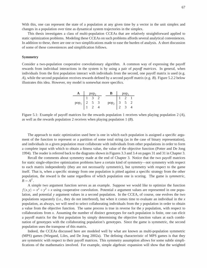
67

With this, one can represent the state of a population at any given time by a vector in the unit simplex andchanges in a population over time as dynamical system trajectories in the simplex.

This thesis investigates a class of multi-population CCEAsthat are relatively straightforward applied tostatic optimization problems. Modeling these CCEAs on suchproblems affords several analytical conveniences.In addition to these, there are one or two simplifications made to ease the burden of analysis. A short discussionof some of these conveniences and simplification follows.

Symmetry

Consider a two-population cooperative coevolutionary algorithm. A common way of expressing the payoffrewards from individual interactions in the system is by using a pair ofpayoff matrices. In general, whenindividuals from the first population interact with individuals from the second, one payoff matrix is used (e.g.A), while the second population receives rewards defined by a second payoff matrix (e.g.B). Figure 5.2.2 belowillustrates this idea. However, my model is somewhat more specifics.

A pop2

1 3 2pop1 2 5 3

1 2 4

B pop1

1 2 1pop2 3 5 2

2 3 4

Figure 5.1: Example of payoff matrices for the rewards population 1 receives when playing population 2 (A),as well as the rewards population 2 receives when playing population 1 (B).

The approach to static optimization used here is one in whicheach population is assigned a specific argu-ment of the function to represent or a partition of some totalstring (as in the case of binary representation),and individuals in a given population must collaborate withindividuals from other populations in order to forma complete input with which to obtain a fitness value, the value of the objective function (Potter and De Jong1994). The reader is referred back to the diagrams shown in Figures 3.3 and 3.4 on pages 31 and 31 in Chapter 3.

Recall the comments about symmetry made at the end of Chapter3. Notice that the two payoff matricesfor static single-objective optimization problems have a certain kind of symmetry—not symmetry with respectto each matrix independently (they are not necessarily symmetric), but symmetry with respect to the gameitself. That is, when a specific strategy from one populationis pitted against a specific strategy from the otherpopulation, the reward is the same regardless of which population one is scoring. The game issymmetric,B = AT .

A simple two argument function serves as an example. Supposewe would like to optimize the functionf (x,y) = x2 + y2 + x using cooperative coevolution. Potentialx argument values are represented in one popu-lation, and potentialy argument values in a second population. In the CCEA, of course, one evolves the twopopulations separately (i.e., they do not interbreed), butwhen it comes time to evaluate an individual in thexpopulation, as always, we will need to select collaboratingindividuals from they population in order to obtaina value from the objective function. The same process is truein reverse for they population, with respect tocollaborations fromx. Assuming the number of distinct genotypes for each population is finite, one can elicita payoff matrix for the first population by simply determining the objective function values at each combi-nation of genotypes with the collaborating population’s genotypes. Since the game is symmetric, the secondpopulation uses the transpose of this matrix.

Indeed, the CCEAs discussed here are modeled well by what areknown as multi-population symmetric(MPS) games (Wiegand, Liles, and De Jong 2002a). The definingcharacteristic of MPS games is that theyare symmetric with respect to their payoff matrices. This symmetry assumption allows for some subtle simpli-fications of the mathematics involved. For example, simple algebraic expansion will show that the weighted

68

average payoff of the first population is the same as that of the second,~x ·A~y = ~y·AT~x. In the game-theoreticframework, the genotypes from thex population determine which row of the payoff matrixA will be used, andgenotypes from they population to determine which column ofA will be used.

Another advantage to this approach is that it provides a certain clarity with respect to the algorithm’s coop-erative nature. When rewards are symmetric between two distinct populations, there can be no doubt that theproblemis cooperative by nearly any definition. Individuals from the two populationscan onlysucceed or failtogether, due specifically to the symmetry. While it may not be true that cooperative coevolutionary algorithmsmusthave a symmetric payoff, it is almost certainly true that anymulti-population coevolutionary algorithmwith symmetric rewards between the populationsis cooperative. This allows me to avoid the debate discussedin Chapter 3 entirely: these algorithms are definitely cooperative ones.

Model Assumptions & Simplifications

With an EGT model comes a variety of simplifying assumptions, several of which have already been touchedupon. For example, it has already been stated that the model assumes that populations are infinite in size. Thisassumption, while certainly important and restrictive, isnot as naive as it might first appear. First of all, themodel can be expanded in the future to consider populations of finite size by modeling populations assamplesof the infinite population. Existing Markov model theory canthen be applied to these augmented systems (Vose1999; Schmitt 2003; Liekens, Eikelder, and Hilbers 2003). Second, there has been some study suggestingthat finite population models with very large population sizes approximate behaviors of infinite population ECmodels (Vose 1999), albeit the meaning of the word “large” has admittedly only been investigated in certainconstraining circumstances (Rabani, Rabinovich, and Sinclair 1998; Schmitt 2001).

Another simplification mentioned above is that the model presented here specifically describes dynamicsfor only two populations. While this again may seem an extreme simplification, it should be noted that theoriginal intent of this work was to lay a foundation of study,and that this foundation would, by definition, beginwith simpler systems for which behavioral understanding ismore tractable. Multi-population models becomecomplicated quickly, both in terms of their demands on our intuition, as well as the mathematics involvedto model them. Modeling CCEAs with two populations is a reasonable way to gain a better fundamentalunderstanding of the behavior of these algorithms.

In addition to these two issues, assumptions must be made as to how individuals interact in order to obtainan assessment of fitness. Although many kinds of interactions are possible, I will retain the standard EGTassumption ofcomplete mixing. This means that during the evaluation phase of the algorithm, individualsin one population are assumed to have interacted with all members of the alternate population in pairwisecollaborations, and vice-versa. To be clear, here the word “mixing” refers to how individuals interact, notvariation. However, unless it is otherwise stated, the reader should assume that references to the word “mixing”refers to variation. With complete mixing, one not only evaluates a given member ofx with every member ofy for collaboration purposes, but also takes the average of the resulting fitness values. Other mixing methodsare often used in practice (see Chapter 4 of this dissertation, for example) due to the computational difficultiesthat arise from this method; however, the theoretical modelis complicated by such methods because they canintroduce discontinuities and other complexities. Analysis that relaxes this assumption is the topic of futureresearch; however, several alternative mixing models are presented at the end of this chapter as a first steptoward such an analysis.

Parents in the CCEA modeled here are chosen using proportionate selection. In this case the algorithmis generational1. It should be noted that the EGT framework allows for analysis of coevolution using otherselection methods (Ficici and Pollack 2000b).

One final important difference between the algorithm described so far and the model about to be presentedshould be discussed. Recall that the abstract CCEA presented in Chapter 3 on page 29 issequentialin the sense

1In a generational EA a new population entirely replaces the old population in a given step, while in a steady state EA each stepreplaces only one parent with one child.

69

that each population is processed and updated in a particular order. The EGT model that follows performs suchan update simultaneously, so reflects aparallel update mechanism. That is, generations for the first populationand the second population are processed at the same time, using information from the previous round. Thenet effect is that changes in one population in the middle of around cannot affect the other population insuch a model. Since both are legitimate implementation choices for the CCEA, and since there are reasons tobelieve that many CCEA properties are general between the two (Jansen and Wiegand 2003c), this is reasonablemodeling choice.

The MPS Model

I now define the MPS dynamical system specifically, initiallywithout variational operators. A round consistsof two phases for each population: fitness assessment and selection. At an abstract level, one might write theequations as a composition of these two phases for each population. The equations below show this abstractionusing the notationF to represent a function that assigns some vector of relativefitnesses to the strategies andthe notationS to represent a function for selection. Note that selection must consider fitnessand the populationvector itself.

Gx = S (Fx,~x) (5.1)

Gy = S (Fy,~y) . (5.2)

Biologists and economists have a more specific form of this abstraction, defined by what they callreplicatordynamics(Weibull 1992; Hofbauer and Sigmund 1998). I make use of thismodel, in discrete time form, inorder to describe the CCEA in the following way. Given two populations,(~x,~y) ∈ ∆n×∆m, representing ratiosof genotypes in two infinite populations, the following equations are used to define the dynamical system for acooperative coevolutionary algorithm (without variation) operating on these populations:

~u = A~y (5.3)

~w = AT~x (5.4)

x′i =

(

ui

~x·A~y

)

xi (5.5)

y′i =

(

wi

~x·A~y

)

yi (5.6)

where~x′ and~y′ represent the new population distributions for the next generation. A and AT describe thepayoffs associated with each pair of possible interactions. This more specific model relates to the abstract onein a straightforward manner. Given the payoff matrixA,~u = Fx(~x,~y) and~w = Fy(~x,~y)

For completeness, it should be noted that frequently an additive constant appears in the first equation,~u = A~y+ ωo, whereωo = 1−min(A), as well as a similar constant for the second equation. Theseconstantsare used to make sure elements of~u and~w are non-negative so that under proportionate selection thesystemremains invariant in the simplex. That points remain in the unit simplex as trajectories are advanced throughthe replicator dynamics. To keep the model simple, the payoff matrices will contain only positive values. As aresult, the constants are not really necessary and will not be used.

Though variation is omitted here, it will be discussed laterin the chapter.

5.2.3 Term, Tools and Problems

Before conducting the analysis, some further groundwork must be established. I begin by providing moreexplicit definitions for terms that are important for the discussions relating the dynamical systems ideas to thealgorithm being modeled. After this, I present two specific tools that I will use to help augment formal analysis:rain-gauge validation and trajectory visualization. Finally, I describe some useful problem domains.

70

Terms and Concepts

One of the benefits of having a more rigorous description of the CCEA is that it provides the opportunity to bemore specific in describing intuitive ideas. Let’s begin by making it clear what we mean by several commondynamical systems terms.

Definition 23. Given a function f: S→ S, a point s∈ S is said to be afixed pointif f (s) = s.

Definition 24. TheEuclidean lengthof a vector~x = 〈x1, . . . ,xn〉 ∈ Rn is ‖~x‖ =

√

x21 + · · ·+x2

n. Let

v = 〈v1, . . . ,vn〉 ∈ IRn, and letε be a positive number. Theε-neighborhoodNε(v) is the set~x∈ IRn : ‖~x− v‖ < ε, the set of points within Euclidean distance ofε of v.

Definition 25. Let f be a map onRn and letv∈ IRn be a fixed point. If there is anε > 0 such that for all~x intheε-neighborhood Nε(v), limk→∞ f k(~x) = v, thenv is astable fixed point.

Definition 26. Let there be a function f: S→ S and a fixed point s∈ S, f (s) = s. We define the set B(s) ⊂ Sto be the set of initial points in S that eventually map to the sfixed point. The set defined by B(s) isconsidered thebasin of attractionof s.

In conjunction with the dynamical systems terms, it is necessary to clarify some basic game-theoretic terms,as well. For example, the termpure strategyrefers to a population vector that is at a basis vector (~x = ~ei ,whereei = 1 and∀ j 6= i,ej = 0). For clarity I will distinguish non-pure strategy population vectors by theterm polymorphic. In order to keep the notation clean and simple, the term ¯v is used to refer to a fixed point(~x,~y) ∈ ∆n×∆m, whether polymorphic or not.

Perhaps the most important game-theoretic term that must bedefined is that of Nash equilibrium (Nash1950).

Definition 27. A pure Nash equilibriumof a two player, strategic game is a pure strategy s∗i, j such that for

every player i∈ I we have:

πi(

si, j ,s∗¬i, j

)

≤ πi(

s∗i, j ,s∗¬i, j

)

, ∀si, j ∈ Si

A Nash equilibrium is considered astrict Nash equilibriumif it is unique, that is the inequality isstrictly >.

Less formally, a Nash equilibrium is a point such that, if either population adopts the strategy associatedwith the equilibrium, the interacting population cannot get a better payoff than to also play at the Nash point.As a result, the best course of action for both populations isto play at a Nash equilibrium (there may be morethan one). The basic idea of this definition is the same for polymorphic Nash equilibria.

All of this terminology from the mathematical tools is useful, but there is still the question of how to relatethe mathematics to the study of the algorithm in ways that address the fundamental question. For instance, whatdoes it mean for such a system to “converge”, or to “nearly converge”? In the previous chapter, the run timeanalysis viewpoint seems to suggest that convergence occurs with first hitting time: the algorithm has convergedwhen it has first reached the global optimum. While this is a useful viewpoint for that kind of analysis, it isnot consistent with the way most practitioners use the term.Since EAs have no guarantee of finding the globaloptimum in some fixed budget of time, real-world applications seldom consider the algorithm in terms of itshaving run until the global optimum is reached (even if it were known). Generally practitioners refer to the termloosely to mean the event that occurs when there is very little diversity left in the system, and objective progressseems to have stalled. In this dynamical systems context thetermconvergencecan be defined as follows.

Definition 28. A population vector,~x, in a CCEA hasconverged, or converged to homogeneity, when it isrepresented by some basis vector.~x hasnearly convergedwhen there is some very small, positiveconstantε such that‖x−ei‖ < ε.

An algorithm hasconvergedor nearly convergedwhen all its populations have done so.

71

When populations~xand~yhave both converged, I say that the those populations areassociatedorcorrespondwith a payoff valueai, j ∈ A, when~x·A~y = ai, j . When a CCEA has converged to a basis vector associated withthe maximum value in the payoff matrix, I say that it hasconverged to the global optimum. The example belowshows a sample payoff matrix with a maximum value of 5. The pure strategy population vectors~y=~x= 〈0,1,0〉correspond with this global maximum.

A pop2

1 3 2pop1 2 5 3

1 2 4

Figure 5.2: This figure demonstrates an example payoff function with a maximum value of 5. The pure strategypopulation vectors~y =~x = 〈0,1,0〉 correspond with this global maximum.

Modeling Iteration: Validation and Visualization

In the previous chapter all analysis was conducted directlyon the actual algorithm. In an effort to provide amore general theory for understanding CCEA behavior, this chapter instead analyzes amodelof the algorithm.Specifically, it analyzes this multi-population symmetricEGT model we’ve discussing. It isn’t always clearhow closely the model matches the real algorithm, or perhapsmore foundational what the mathematical resultsmeanin terms of the real algorithms.

To help bridge this gap, it is often useful to take the mathematical model anditerate it. By this I mean picka random initial condition and apply the model repeatedly until I believe some limit behavior has been reached.How this end point is determined is a relatively complicatedquestion, which I will forgo for the moment. Theresult of this iteration is atrajectory through the Cartesian product simplex space, as well as the fixed pointresting place of the trajectory. With these pieces of information, projections of the trajectories can be visualizedand the basins of attraction can be measured. These two toolswill help us understand some of the connectionsbetween the model and the real algorithm at a less formal level.

I have defined the term basin of attraction in the usual way: the basin of attraction of a given fixed point,or any limiting behavior, is the set of initial points that will eventually map to that point, or appropriate limitbehavior. Measuring the sizes of the basins of attraction ofall the various limiting behaviors of a dynamicalsystem is difficult. First of all, there is no guarantee that there is any general analytical way to do so. Second,it is typically difficult to definitivelyknowall the possible limiting behaviors, much less measure their basins.Moreover, the dimensionality of the spaces of the systems inwhich I am interested are very large, so evenwhen restricting attention to just the fixed points, assuming there are no cyclical or chaotic orbits, the space ofpotential attractors may be quite large. Fortunately, as wewill shortly see, the results of my analysis will allowme to make this more tractable. This will be discussed in moredetail after the analysis.

To estimate the size of a basin of attraction the simple method called arain gauge measure(Alligood, Sauer,and Yorke 1996) is used. An initial point is selected uniformly at random from the product simplexes usingZuev’s method (Zuev and Kahan 2001), a trajectory through the space is computed using the initial point, thesystem is iterated some large number of times, then the limiting behavior is examined. In my case all trajectoriesmove to a finite set of known potential fixed points, so I maintain a histogram corresponding to these points.If the trajectory seems to have converged “very close” to a particular basis vector, I increment its value in thehistogram. I then repeat this process some large number of times (5000).

While the condition “very close” is somewhat qualitative, and ingeneralmay not be sufficient (e.g., unstablepoints will push points that are “very close” away), wecanbe more comfortable with this choice if an observed

72

trajectory approaches a known stable fixed point (which willbe shown in this case). Validation studies of thisnature were run for 2000 iterates, or until they were “very close” meaning within a delta of 10−4 in terms ofvariational distance. All iterates in this work met this latter criterion.

Iterating the model not only offers the opportunity to assess the relative sizes of the basins of attraction,an additional benefit is its ability to help us visualize and characterize the trajectories themselves. This can bedone by plotting something similar to the so-calledtakeover curvesused for standard GA analysis (Goldbergand Deb 1990). However, in this case the curves must be two dimensional in order to capture both populations.The plots are constructed by first identifying which genotypes correspond with the maximum payoff value ineach population and plotting over time the proportions of these genotypes in their respective~x and~y populationvectors. This can be seen as a top-down view of these two-dimensional takeover curves.

With these two tools, one can gain intuition about a number ofthings. First of all, with the visualization wecan gain some limited understanding of what the population itself is doing during the search: where it is goingand how various algorithmic and problem characteristics are affecting this trajectory. Second of all, with thevalidation we can gain some perspective on how likely trajectories are to move to particular fixed points. Thishelps connect us to the real algorithm by addressing the question of likelihood of global convergence.

Problem Domain

In order to conduct an analysis, I will need to do so in the context of problems or, at the very least, propertiesof problems. Thus, it is necessary to explain how a simple encoding of a static optimization problem can bemapped into this EGT model context. The process is quite simple.

Any two argument function can be mapped into a payoff matrix for a two population symmetric game(Wiegand, Liles, and De Jong 2002a). Doing so only requires an assumption that the fitness space is discrete.A matrix can be produced by simply enumerating all genotypicvalues for one population along the rows, andall genotypic values for the second population along the rows, and evaluating the given function at each orderedpair. In practice this process would be absurd (since enumerating the space would solve the optimizationproblem), but here the idea is an abstraction for the purposeof theoretical research.

Let us start with a straightforward problem for which it is easy to gain some intuition, and for whichvisualization is tractable, a simple 2D parabolic function, SIMPLEQUADRATIC .

Definition 29. Given a constant offset k and a location for the center peak(xc,yc), the functionSIMPLEQUADRATIC : N×N → R is defined by

SIMPLEQUADRATIC (x,y) = k−[

(xc−x)2 +(yc−y)2] .

In my case, the domain values for both arguments are in the interval [1,8]. To be specific, let us say that themaximum value,k = 100, is found near the center of the bowl—located at(xc,yc) = (4,4). In all cases eachargument has eight distinct genotypes represented by both populations, making a 8× 8 payoff matrix (whenvariation is considered, this can be seen as being represented by 3-bit strings each). The figure below illustratesa surface plot of this function, as well as the payoff matrix elicited by this objective function.

This landscape is helpful precisely because of its simplicity. While it is simple, there are still interestingobservable phenomena when the CCEA is applied to it, as will be clear when we look at the effects variationhas on CCEA dynamics. Further, in these cases the unimodality of the simple 2D parabolic function allowsmore complicated dynamical behaviors (such as convergenceto suboptimal, local peaks) to be ruled out as ameans of explaining some of these effects.

A somewhat more interesting object of study is the MAX OFTWOQUADRATICS landscape, which presents abimodal problem. This problem retains much of the simplicity of the SIMPLEQUADRATIC in terms of analysis,while adding the additional complexity of having two peaks.This provides the possibility of converging to asuboptimal peak in the landscape. I define a broad class of configurable landscapes below.

73

12

34

56

78

0

2

4

6

865

70

75

80

85

90

95

100

A pop1

82 87 90 91 90 87 82 7587 92 95 96 95 92 87 8090 95 98 99 98 95 90 83

pop2 91 96 99 100 99 96 91 8490 95 98 99 98 95 90 8387 92 95 96 95 92 87 8082 87 90 91 90 87 82 7575 80 83 84 83 80 75 68

Figure 5.3: This figure depicts the SIMPLEQUADRATIC function pictorially (left), as well as the payoff matrixit elicits (right). The global maximum appears in bold in thepayoff matrix.

Definition 30. Given constant values defining the two peaks: k1 and k2 to define the peak heights, s1 ands2 to define the peak width, as well as(x1, y1) and(x2, y2) to define the locations of the peaks, the functionMAX OFTWOQUADRATICS : N×N → R is defined by

quad1(x,y) = k1−s1 ·[

(x1−x)2 +(y1−y)2]

quad2(x,y) = k2−s2 ·[

(x2−x)2 +(y2−y)2]

MAX OFTWOQUADRATICS(x,y) = max(quad1,quad2)

The useful thing about this function class is that the problem can be tuned in such a way that the globalpeak covers much of the domain, covers an equitable portion of the domain, or covers very little of the domainrelative to the local peak. This allows one to define specific landscapes where the globally optimal and locallysub-optimal peaks have different attracting potential. The parameter settings for MAX OFTWOQUADRATICS

used for my investigations are defined in Table 5.2.3 on page 74.The value fors1 will be varied in order to control relative amount of coverage the two peaks have over the

domain. The two figures on page 74 show two different instantiations of this problem class, at the extremesof s1. The first provides one in which the global and local peaks cover more or less comparable areas of thedomain, while the second shows a landscape with a broad suboptimal peak and a narrow global peak.

5.3 Dynamical Systems Analysis

With this model, and these definitions in place, the fundamental question can now be stated much more specif-ically: “Are CCEAs generally predisposed to converge to theglobal optimum?” Rephrased, this can be statedas follows. Starting in an arbitrary spot in the Cartesian product simplex, are trajectories likely to converge tohomogeneity at, or near, the basis vector associated with the maximum payoff value? For dynamical systemsmodels, this raises such questions as what points in the space are fixed points, what is the stability of those fixedpoints, and what is the relative size of basins of attractionof such points?

The remainder of this chapter will focus on attempting to answer questions about these characteristics withthe tools I mentioned above, both without and with variational operators. I begin with the model as it as alreadybeen presented, without variation.

74

Table 5.1: This table describes the parameter settings usedfor the MAX OFTWOQUADRATICS function.

Parameter Value(s)k1 100k2 75s1 2,4,8,16,32,64s2 1

(x1, y1) (8,1)(x2, y2) (1,8)

12

34

56

78

0

2

4

6

820

30

40

50

60

70

80

90

100

A pop1

26 28 50 68 82 92 98 10039 38 48 66 80 90 96 9850 49 46 60 74 84 90 92

pop2 59 58 55 50 64 74 80 8266 65 62 57 50 60 66 6871 70 67 62 55 46 48 5074 73 70 65 58 49 38 2875 74 71 66 59 50 39 26

Figure 5.4: This figure depicts the MAX OFTWOQUADRATICS function withs1 = 2 pictorially (left), as well asthe elicited payoff matrix (right). The global maximum appears in bold in the payoff matrix.

0

2

4

6

8

12

34

56

780

20

40

60

80

100

A pop1

26 25 22 17 10 1 36 10039 38 35 30 23 14 3 3650 49 46 41 34 25 14 1

pop2 59 58 55 50 43 34 23 1066 65 62 57 50 41 30 1771 70 67 62 55 46 35 2274 73 70 65 58 49 38 2575 74 71 66 59 50 39 26

Figure 5.5: This figure depicts the MAX OFTWOQUADRATICS function withs1 = 64 pictorially (left), as wellas the elicited payoff matrix (right). The global maximum appears in bold in the payoff matrix.

75

5.3.1 Analysis without Variation

The goal of this section is to communicate a better understanding CCEA dynamics by analyzing the correspond-ing MPS models from a dynamical systems perspective. In particular, the focus is on population trajectories,the existence and location of fixed points and their basins ofattraction. I summarize what is known for MPSmodels without variation, set the stage for studying the effects due to variation, and address questions aboutwhere fixed points are, and when they are stable.

Stability of Fixed Points

If variation is excluded, there is much that can be said analytically about MPS models. For example, anystrict Nash equilibria (see Definition 27 above) must contain only pure strategies; that is, they must be at thebasis vectors, the corners of the simplexes (Hofbauer and Sigmund 1998). This means that in the absence ofvariational operators, one can expect the populations in these systems to converge to homogeneity. It is alsoknown, however, that mixed strategy equilibria are possible on the bnd(∆n×∆m) when the Nash points are notstrict. This can happen when there are plateaus or ridges in the objective landscape, for instance.

Indeed, there’s much that can be understood about the limiting behavior of these algorithms from this model.Below, I present proofs of some useful properties about discrete time MPS systems as models of CCEAs appliedto static optimization. These proofs are very instructive.From them several things are shown about when basisvector fixed points are purely stable and purely unstable. Inaddition, a basis is provided for understandinghow certain kinds of local convergence problems can occur ina CCEA, even with infinite populations and novariation.

However, before beginning, some context and plan for the proofs should be established. The intent is tobe able to make some general statements about theJacobianof the system of equations generated by algebraicexpansion of the replicator and selection equations (See Eq. 5.3–5.6 on page 69) evaluated at fixed points, ¯v thatare associated with the corners of the simplex. Since one canshuffle rows and columns of the payoff matrix andthe game remains the same, without loss of generality I restrict the discussion to the case where ¯v correspondswith the elementa1,1 in theA payoff matrix. A can be expressed as shown below. All other cases follow as aresult.

A =

a1,1 a1,2 · · · a1,n

a2,1. . . · · · a2,n

......

an,1 · · · an,n

(5.7)

I start by showing that there are particular patterns that will necessarily be found in theJacobianwhenevaluated at the fixed point,Jv(va1,1). This structure allows me to make assertions about the eigenvalues of theJacobianin the general case. These steps lead directly to a theorem that explains that the fixed point associatedwith the maximum value in the payoff matrix is always stable.Several corollaries follow directly from thistheorem that give more information about the nature of stability in basis vector fixed points.

Lemma 1. Let Jv be theJacobianof the system of equations generated by algebraic expansionof thetwo-population, n-strategy evolutionary game, where A is the payoff matrix and the replicator equationsare given in Equations 5.3 – 5.6. Given the fixed pointva1,1 associated with the a1,1 item in A, theeigenvalues of theJacobianevaluated at theva1,1 fixed point, Jv(va1,1), are the diagonal elements.

76

Proof. The proof begins by partitioningJv(va1,1) into four partitions. These partitions are used to show thatJv(va1,1) must be in a particular form, then conclude it by proving thatlemma 1 follows as a result of this form.

Jv(va1,1) can be partitioned into four equal sized partitionsB, C, D, andE shown in equation 5.8 below.

Let partitionB of the Jacobiancorrespond to all∂x′i∂xj

, C to ∂x′i∂yj

, D to ∂y′i∂xj

, andE to ∂y′i∂yj

. Let’s begin with theBpartition.

Jv(va1,1) =

[

B CD E

]

(5.8)

The nth column and row from the matrix are omitted. This can be done because thexn variable may bere-written using the other components in~x (that is,xn = 1−∑n−1

i=1 xi), and because the new proportion for thexn component in the next generation is fully specified by the equations without the redundantx′n. Of course, asimilar argument holds for thenth column and row of all four partitions.

The algebraic form ofui = ai,1y1 + ai,2y2 + · · ·+ ai,(n−1)y(n−1) + ai,n

(

1−∑n−1i=1 yi

)

can be obtained from

equations 5.3 and 5.4. In theB partition case the partials are taken with respect to one of the~x variables, so the~y values can be substituted from ¯va1,1 since they will be considered constants in the derivatives.This providesa somewhat simpler algebraic form to use:ui = ai,1y1 + ai,n(1− y1) = ai,1. Most of the~x values may also besubstituted as constants as long as the partial derivativescan still legitimately be taken. Elements that fall inthe ith row or jth column, as well as those in the first column and row are preserved in order to examine thepartial—all other values in~x are zero, so further simplification is possible. Thex′i algebraic form is shownbelow.

x′i =ai,1xi

x1ai,1 +xi(ai,1−an,1)+x j(a j,1−an,1)

If i 6= j then one can substitute either 0 or 1 forxi when taking the partial with respect tox j . If i 6= 1, then

it is true that∂x′i∂xj

= 0 since the numerator will remain a zero factor after the derivative. Therefore it can be said

that all elements in theA partition ofJv(va1,1) are zero as long asi 6= j and i 6= 1. The form of the partition isshown below in equation 5.9.

Jv(va1,1) =

j1,1 j1,2 · · · j1,n−1

0 j2,2 0 · · ·... 0

... 0

(5.9)

By symmetry theE partition has the same form.TheC andD partitions never havei = j, so their diagonals are always zero. There is only one case for

these partitions that remains to be considered: wheni = 1. This is dealt with by first taking thei = 1 case forC and returning to the replicator function to get the following algebraic expression after appropriate constant

substitutionsui = ai,1 +ai, jy j −ai,ny j . After simplification, the selector equation is thenx′i =xi(ai,1+ai, j yj−ai,nyj)x1(ai,1+ai, jyj−ai,nyj)

.

The terms in the numerator and denominator cross out wheni = 1 and becomes constant, the partials of whichare zero. Thus all elements in theC partition (andD by symmetry) are zero.

Now that the structure ofJv(va1,1) is known, consider the eigenvalues of this matrix. Recall that to computethis, the characteristic equation must be solved such that det

(

Jv(va1,1)−λI)

= 0. One can compute this byexpansion of cofactors on the first column. From the above discussion it is known that the first column of theJacobianare all zeros except elementsj1,1. The cofactors ofj1,1 is the product of the diagonal termsJv(va1,1)excluding j1,1. This can be seen by repeated application of the expansion ofcofactors.

Thus, the determinate is simply the product of the diagonal terms of the matrixJv(va1,1)−λI , and the roots of the characteristic equation will be the diagonal elements of theJacobian. There-fore the eigenvalues ofJv(va1,1) are its diagonal elements.

77

Lemma 2. Given Jv(va1,1), the following properties are true.

∂x′i∂x′i

(

va1,1

)

=ai,1

a1,1∀i 6= 1 (5.10)

=an,1

a1,1i = 1 (5.11)

∂y′i∂y′i

(

va1,1

)

=a1,i

a1,1∀i 6= 1 (5.12)

=a1,n

a1,1i = 1 (5.13)

(5.14)

Proof. Again, begin with partitionB of Jv(va1,1). Returning to the replicator Equation 5.6 after appropriateconstant substitution providesui = ai,1y1 +ai,n(1−y1) = ai,1. There are two cases:i 6= 1 andi = 1. In the fistcase, again retainingxi for the partial, the remaining values for~x are substituted as constants and obtain thefollowing selection equation and subsequent partial derivation.

x′i =xiai,1

x1a1,1 +xi(ai,1−an,1)

∂x′i∂x′i

(

va1,1

)

=ai,1x1a1,1

(x1a1,1 +xiai,1−xian,1)2

=ai,1

a1,1

In the case wherei = 1, xi is not preserved, so the following is obtained after relevant substitution.

x′i =x1a1,1

x1a1,1 +an,1−x1an,1

∂x′i∂x′i

(

va1,1

)

=a1,1an,1

(an,1−a1,1−an,1)

=an,1

a1,1

The proof for the∂y∂i i case can be obtained from theD partition by symmetry.

Theorem 5. Let m be a unique maximum value in A, m= max(A). Given a non-polymorphic fixed pointv,if the payoff value ai, j = m andv corresponds with ai, j , thenv is a stable fixed point.

Proof. Givenai, j = mand thatai, j can be moved into positiona1,1, then all eigenvalues are< 1 by lemma 2.

Noting in lemma 2 that all the eigens for a particular ¯v are ratios ofA values at some fixed column or row,and applying the same juxtaposition logic from Theorem 5, several interesting corollaries can be derived. Forexample, it follows directly that anyai, j that is the unique maximum value of theith row and jth column ofAis also a stable fixed point. Additionally, anyai, j that is the minimum value of theith row and jth column ofAis a purelyunstablefixed point (meaningall its eigenvalues are> 1). With these, I can bound the number ofstable and unstable basis vector fixed points in the system ingeneral. These corollaries are stated more formallybelow.

Corollary 1. From Theorem 5 it follows directly that if

ai, j > al , j ∀l 6= i, and

ai, j > ai,k ∀k 6= j,

thenvai, j is a stable fixed point.

78

Corollary 2. As per corollary 1, lemma 2 and theorem 5 dictate that if

ai, j < al , j ∀l 6= i, and

ai, j < ai,k ∀k 6= j,

thenvai, j is a purely unstable fixed point. The global minimum value,min(A) is always purely unstable.Additionally any other fixed points at the corner of the simplex which are neither purely unstable norstable will be an unstable saddle point.

Corollary 3. From corollaries 1 and 2 we also know that the maximum number of stable basis vector fixedpoints is n and the minimum number of stable basis vector fixedpoints is1. The same rule is also truefor the number of purely unstable fixed points. Therefore thenumber of unstable saddle basis vector fixedpoints must be at least n2−2n.

What does this analysis explain about convergence and optimization? As I made clear in Definition 28above, when trajectories limit to a fixed point at the basis vector, this corresponds to the populations becominghomogeneous. The question is, where can this occur in terms of the fitness landscape? Recall that in our MPSmodel of cooperative coevolution, the payoff matrix is really just a quantized version of the fitness landscape.Given this, perhaps the most important thing worth noting isthat a form of local convergence is possibleeven with an infinite population, no variation, and unique values in the fitness landscape. Trajectories can fall tobasis vectors that correspond with suboptimal fitness values. This is not possible in the simple genetic algorithmunder the very same assumptions (Reeves and Rowe 2002; Vose 1999).

However, knowing the stability of a fixed point in a system does not necessarily indicate how likely it willbe reached by any arbitrary initial condition, unless more is known about the dynamical system (Hofbauer andSigmund 1998). Fortunately, even without the deeper understanding required for formal proofs, considerableinsight into these issues can be obtained using the model validation and visualization techniques discussedearlier. In the following section I summarize these insights for MPS models without variation.

Population Trajectories and Basins of Attraction

Let us now turn to the visualization and validation tools mentioned previously to help clarify the meaning ofthe formal results. Recall that visualization of these systems involves iterating the model until the fixed point isreached, then displaying its trajectory in terms of a projection offered by looking only at the component vectorsassociated with the global maximum. The visual effect corresponds to a form of 2D takeover curve and helpsone understand where trajectories are going relative to theglobal peak. A rain-gauge measure can be taken forthe relative sizes of the basins of attraction of the fixed points by doing this many times and recording wherethe final resting points.

Of particular interest is the size of a fixed point’s basin of attraction relative to the other fixed points towhich trajectories go. Since I’ve now some idea that these are very likely to be basis vectors (in the absenceof variation), the question of global convergence can be addressed in a way that makes sense relative to theproblem space itself. In other words, viewing convergence to a basis vector as a collapse to homogeneity inboth populations and knowing the relative sizes of the basins of attraction of each possible pair of homogeneouspopulations should give us insight into how likely it is thata pair of random initial populations will converge tosome particular pair of homogeneous populations.

Indeed, there is reason to believe that the size of the basinsof attraction of a fixed point indicated by abasis vector has more to do with relative local column and rowvalues in the payoff matrix than how large thespecific payoff value is at that point. The idea is that thejoint distribution of the rewards for a given strategyin one population as defined by the set ofpossiblecollaborating strategies from the alternative populationismore attractive for trajectories than thespecificvalue of the optimal collaboration for that strategy. In otherwords, broad and suboptimal peaks will pull trajectories away from taller, more narrow peaks. This is the form

79

of local convergence in CCEAs mentioned above, and touched upon in other studies (Ficici and Pollack 2000c;Wiegand, Liles, and De Jong 2002a).

Recall that measuring the basins of attraction can be quite complicated in general. In this case though, thereare three things we know, or can do, to make this a more tractable problem. First, some useful properties arealready known about these systems that help. For instance, it is known that as long as the maximum values onthe rows and columns are unique, the only strict Nash equilibria are at the basis vectors. Second, knowing this,I can construct a problem such that this property is true of mypayoff matrix. Finally, I can apply the validationmethod already discussed in order to obtain this measure.

As an example, consider the SIMPLEQUADRATIC function previously discussed. In particular, I take the8×8 payoff matrix elicited for this function and iterate the MPS model many times until convergence is reached.Having done so, the expected result that all trajectories lead to the basis vector fixed point associated with theglobal optimum was obtained. That is, when an initial starting state for the populations is chosen at random, themodel predicted that a CCEA algorithm will converge to homogeneity at the global maximum of this function.

Figure 5.6 illustrates this for several example trajectories. Each curve begins at the point indicated by ahollow circle, and terminates at the point indicated by an “x” (in this case all of these terminate in the corner).Every 100 steps of the trajectory are marked on the curves to get an idea of the rate of progress of the curves,though all points on the plot represent steps produced by themodel. Trajectories that converge near the globaloptimum appear as thicker lines than those that do not. In this way, one can track the proportions of the com-ponents associated with the maximum value over time as they move from the initial population configurationstoward its ultimate limit behavior. Asymmetries in the projected trajectories are due to asymmetric differencesin the sample of initial points or asymmetries that exist in the function itself (the latter of which, in this case,are minimal).

0.0 0.2 0.4 0.6 0.8 1.0

0.0

0.2

0.4

0.6

0.8

1.0

Xmax

Ym

ax

++++++++++++++++++++x

++++++++++++++++++++x

+

+++++++++++++++++++x

+

+++++++++++++++++++x+ +++++++++++++++++++x

+

+++++++++++++++++++x

+

+++++++++++++++++++x+ +++++++++++++++++++x

+

+++++++++++++++++++x

++++++++++++++++++++x

++++++++++++++++++++x

++++++++++++++++++++x

+

+

++++++++++++++++++x+

+++++++++++++++++++x+

+++++++++++++++++++x

Figure 5.6: 2D Takeover plot for trajectories operating on the simple quadratic problem with no variation.Curves begin at points indicated by hollow circles, and terminates at the point indicated by an “x”. Every 100steps of the trajectories are marked.

The result of the of this is expected. But what of the fact thatanalysis reveals that there can be otherstable basis vector fixed points than the one associated withthe global maximum, and what of the problem ofconsensus caused by cumulative weights along joint distributions in the payoff matrix mentioned in the previouschapter? Indeed, the MAX OFTWOQUADRATICS problem is constructed so that trajectories are more attractedto the suboptimal peak than to the global maximum. This is done by making sure the rows and columnsin the payoff matrix corresponding with the suboptimal local peak are significantly biased over the row andcolumn values corresponding with the global peak. Ranging thes1 parameter in the MAX OFTWOQUADRATICS

problem presented above makes this fact palpably clear.

80

Consider all 6 example functions from the MAX OFTWOQUADRATICS class presented above resulting fromvarying s1 ∈ 2,4,8,16,32,64. Again, I use these functions to elicit 8× 8 sized payoff matrices; however,varying the parameter now results in different amounts of coverage between the two peaks. Table 5.3.1 belowdescribes the percentage of domain that the global peak covers ass1 is increased.

Table 5.2: This table describes the percentage of domain points in MAX OFTWOQUADRATICS that are coveredby the global peak as thes1 parameter is varied.

s1 Coverage of global peak2 43.75 %4 29.69 %8 17.19 %16 12.50 %32 6.25 %64 4.69 %

The rain gauge method described above was also run for each ofthese problems. The result was that in allcases trajectories converged to basis vectors associated with one of the two peaks, but not necessarily the globalpeak. Note that the relative difference in height between the peaks remains the same in all functions, regardlessof s1 (refer again to the figures on page 74).

0 10 20 30 40 50 60

0.0

0.2

0.4

0.6

0.8

1.0

S1

Rat

io C

onve

rged

to M

ax

Figure 5.7: This graph shows the ratio of trajectories that converged to the basis vector associate with the globalmaximum of the MAX OFTWOQUADRATICS function as thes1 parameter is varied in2,4,8,16,32,64.

Looking more closely at where the trajectories are actuallygoing helps these results. Figure 5.8 on page 5.8illustrates trajectory behavior for a subset of the those initial conditions for each of the problems generatedby varyings1. The panels appear in order from left to right, top to bottom.Some minimal amount of initialprobability in the components associated with the global peak is necessary to converge to the global optimum.

81

As the coverage of the global peak diminishes, we begin to seethe effects of the increased attraction to the localpeak. This justifies our intuition that cumulative payoff values local to some suboptimal maxima can distracttrajectories from finding the global peak when they are sufficiently large.

5.3.2 Analysis with Variation

In order to extend the MPS framework to model variational operators, the methods outlined by Vose (1999) havebeen employed. Hence, the dynamical system becomes a composition of the original model and a variationalmixing function,M . For simplicity, I assume that the variational operators are the same for both populationsand the populations have the same number of distinct genotypes, so the sameM can be used for both popula-tions. With these assumptions the abstract formulation of the MPS model now becomes:Gx = M (S (Fx,~x))andGy = M (S (Fy,~y)).

Mixing can be done in any number of ways, so this abstract formulation does not commit to a particularrepresentation; however, to build concrete mathematical models I will need to be more specific—and doingso will imply particular representations for individuals,as well as particular operators. Remaining consistentwith earlier chapters, I assume that the representation is binary, and focus on two common operators for suchrepresentation (one for mutation and one for crossover). The M function is constructed for these operators.

Let’s start by enumerating what the probability is that the all zero string will be produced by any arbitrarypair of individuals acting as parents. It is clear that ann× n matrix, M, results from such an enumeration.Supposing one has such a matrix, obtaining the probability that the all zero string is generated after replicationand variation is a relatively straightforward exercise:

x′′0 =∑

u,v∈Ω

x′ux′vMu,v (5.15)

y′′0 =∑

u,v∈Ω

y′uy′vMu,v (5.16)

Variation works as follows. Parents are selected using Eq. 5.3–5.6. The resulting probabilities are used for~x′ and~y′. TheMu,v value represents the likelihood that the all zero string is constructed or not destroyed whenuandv are parents. Finally, the sum over all such combinations is taken. To produce a value for any child string,not just the all zero string, the mixing matrix is permuted (see Vose (1999) for more details). Given this, thenext generation’s population states (now notated~x′′ and~y′′) can be obtained using the following equations:

x′′k =∑

u,v∈Ω

x′ux′vMu⊕k,v⊕k (5.17)

y′′k =∑

u,v∈Ω

y′uy′jvMu⊕k,v⊕k (5.18)

Computing values for the mixing matrix,M is involved. The reader is referred to Vose (1999) for the deriva-tion and motivation. Given two parents,u andv, what is the probability that the all zero string is constructed, orsurvives? To answer this, we first note that masks can be used to instantiate the effect of a particular crossoveror mutation event. To determine probabilities for a givenMuv, a distribution across all such masks will be nec-essary. To be consistent with existing work, I use the symbolχ to represent the distribution of crossover masksandµ to represent the distribution of mutation masks. Modeling particular genetic operators involves elicitingthese two distributions. The probabilityMuv can be obtained as follows.

Muv =∑

u,v,k∈Ω

µuµvχk + χk

2· I(i, j,u,v,k) (5.19)

I(i, j,u,v,k) =

1 if ((i ⊕u)⊗k)⊕(

( j ⊕v)⊗ k)

= 00 otherwise (5.20)

82

0.0

0.2

0.4

0.6

0.8

1.0

+

+++++++++++++++++++x++++++++++++++++++++x++++++++++++++++++++x

+

+

++++++++++++++++++x++++++++++++++++++++x

+

+

+

+++++++++++++++++x

+

+++++++++++++++++++x

++++++++++++++++++++x

++++++++++++++++++++x

+

+

++++++++++++++++++x

++++++++++++++++++++x++++++++++++++++++++x

+

+++++++++++++++++++x

++++++++++++++++++++x

++++++++++++++++++++x

++++++++++++++++++++x

++++++++++++++++++++x

++++++++++++++++++++x++++++++++++++++++++x++++++++++++++++++++x++++++++++++++++++++x++++++++++++++++++++x++++++++++++++++++++x

++++++++++++++++++++x

+

+++++++++++++++++++x

++++++++++++++++++++x++++++++++++++++++++x

++++++++++++++++++++x

++++++++++++++++++++x

++++++++++++++++++++x0.

00.

20.

40.

60.

81.

0

++++++++++++++++++++x

++++++++++++++++++++x

++++++++++++++++++++x++++++++++++++++++++x++++++++++++++++++++x++++++++++++++++++++x++++++++++++++++++++x++++++++++++++++++++x

++++++++++++++++++++x++++++++++++++++++++x

++++++++++++++++++++x++++++++++++++++++++x++++++++++++++++++++x++++++++++++++++++++x++++++++++++++++++++x ++++++++++++++++++++x++++++++++++++++++++x++++++++++++++++++++x++++++++++++++++++++x++++++++++++++++++++x++++++++++++++++++++x++++++++++++++++++++x++++++++++++++++++++x++++++++++++++++++++x++++++++++++++++++++x++++++++++++++++++++x++++++++++++++++++++x++++++++++++++++++++x++++++++++++++++++++x++++++++++++++++++++x

0.0 0.2 0.4 0.6 0.8 1.0

0.0

0.2

0.4

0.6

0.8

1.0

++++++++++++++++++++x++++++++++++++++++++x++++++++++++++++++++x++++++++++++++++++++x++++++++++++++++++++x++++++++++++++++++++x++++++++++++++++++++x++++++++++++++++++++x++++++++++++++++++++x++++++++++++++++++++x++++++++++++++++++++x++++++++++++++++++++x++++++++++++++++++++x++++++++++++++++++++x++++++++++++++++++++x

0.0 0.2 0.4 0.6 0.8 1.0


Figure 5.8: MPS trajectories on MAX OFTWOQUADRATICS with s1 ∈ 2,4,8,16,32,64. The panels appear inorder, left to right and top to bottom. Open circles represent initial points for trajectories converging to globalmaximum. Closed circles represent initial points bound forsmaller local maximum.

83

The meaning of the indicator functionI described in Equation 5.20 is this: indicate whether or not the all zerostring is formed when thei mutation event mask is applied to parentu, the j mutation event mask is appliedto parentv, and thek crossover event mask is used for the recombination of those two parents. Crossoverproduces two children, sok is needed to represent the reflected side of the recombinatoric symmetry. Themodel assumes only one of the two children is used, thus the expected value is taken between the maskskandk. The reader is referred to Vose (1999) for a more in depth explanation of how these mixing matrices areconstructed for particular operators that are not discussed here. I will illustrate howM can be created using twospecific operators, but first let’s look more formally at the more general MPS model under mixing.

Fixed Points under Mixing

There is little doubt that variational operators significantly change the underlying dynamical system of a CCEA,just as they do in a traditional EA. Not only can the limiting properties of the fixed points of the system change,but the location of the fixed points themselves can change. Tosee this, note that for a fixed point of the MPSmodel toalsobe a fixed point of the variational model, it must be true that~x′′ =~x′ =~x and~y′′ =~y′ =~y. For thepurpose of this fixed point discussion, Equations 5.17 and 5.18 are re-written as follows.

x′′k =∑

u,v∈Ω

xuxvMu⊕k,v⊕k (5.21)

y′′k =∑

u,v∈Ω

yuyvMu⊕k,v⊕k (5.22)

As we saw earlier, the fixed points of MPS models without variation were basis vectors. What happens whenvariation is added? Suppose we are interested in the basis vectors associated with payoff valueapq, that isxi = 0,∀i 6= p,xp = 1 andyi = 0,∀i 6= q,yq = 1. If such is the case, then the resulting values from the aboveequations are always 0, except whenu = v = p for the first case, andu = v = q for the second case. Thus, thenext point in the trajectory, when starting at the basis vector is the following:

x′′k = Mp⊕k,p⊕k (5.23)

y′′k = Mq⊕k,q⊕k (5.24)

There are two important things to note about this observation. First, one can ascertain theG1x (~x,~y),G1

y (~x,~y)step of the MPS model from any arbitrary basis vector pointfrom just the mixing matrix. Second, resultingvalues turn out to be diagonals of thepth andqth permutation of the mixing matrix forGx andGy, respectively.If this diagonal is equal to the original bases, then the fixedpoint of the original system is also a fixed point ofthe system under variation, and if not then it is not. As I willdiscuss in the following sections, this is true foralmost all traditional crossover operators and never true for traditional (non-zero) mutation.

Assessing fixed point stability under mixing is harder than without variation, since the fixed points maynow be in the interior of the simplex product. This means thatit becomes necessary to simultaneously solvethe collective system forGx(~x,~y) =~x andGy(~x,~y) =~y. However, when one is certain that the basis vectors arefixed points, even under mixing, one can evaluate them as I didin the previous paragraph.

Stability of Fixed Points

Unlike the MPS models without variation, the stability of fixed points of the model under variation is a functionof M. Moreover, this dependence is not due simply to the inclusion of M itself into the model, but also from theresulting non-linearity added from the crossover operation. The proof of this is trivial, but I offer it for the sakeof completeness.

Theorem 6. Let v be a fixed point of the cooperative coevolutionary algorithm with variation as described byequations 5.17 and 5.18. The stability of such a fixed point will depend on the specific values in themixing matrix, M.

84

Proof. To assess the stability of a fixed point, one must first know what the fixed point is. While some of thefixed points are known for crossover, this is not necessarilytrue for mutation (or for mutationand crossover).Still, assuming one knew what the fixed point was, theJacobianof the system could be evaluated at that fixed

point. Let’s look at one term∂x′′k∂xl

, but first let’s expand and re-write the equations 5.17 and 5.18. The variablefis used for the convenience of notational simplification only.

x′′k =∑

u,v∈Ω

(A~y)uxu(A~y)vxvMu⊕k,v⊕k

(~xTA~y)2

=

∑

u,v∈Ω(A~y)vxu(A~y)vxvMu⊕k,v⊕k

(~xTA~y)2 =f

(~xTA~y)2

∂x′′k∂xl

=

∂ f∂xl

·(

~xTA~y)2− f · ∂

∂xl

(

~xTA~y)2

(~xTA~y)4

=

∂ f∂xl

·(

~xTA~y)2− f ·2

(

~xTA~y)

(A~y)l

(~xTA~y)4

Taking the partial off now results in the following.

(A~y)l

∑

i∈Ω,i 6=l

(A~y)ixl Mi⊕k,l⊕k +2(A~y)2l xl Ml⊕k,l⊕k

By symmetry, the same is true for∂y′′k∂yl

. From this we learn that both terms in the numerator depend onvaluesfrom M, and that they cannot be eliminated.

Although this was perhaps already obvious, the proof is instructive since it illustrates the fact that the non-linearities introduced by equations 5.17 and 5.18 presentsa far more complicated expression that requires thatchange in any given component depends on all the components from both populations. This differs from themodel without variation, since in that case taking the derivative eliminated all components of one populationfrom the expression. Therefor, its dependence is due not just to the explicit presence of the values inM, butalso due to the non-linearities created by its inclusion.

Parameterized Uniform Crossover

Let’s look at the effects of crossover alone. In this case, for most types of crossover, the probability of obtainingsome stringk when crossing over two identical parents is 0 unless the parents are themselvesk. Whenkis crossed-over withk, the probability that the resulting child is alsok is 1. Thus the diagonal of thekth

permutation ofM is always 1 atmkk and zero elsewhere. This implies that the pairs of basis vectors formingfixed points of the MPS model without variation are still fixedpoints under crossover. This is consistent with anunderstanding of the effect of crossover on a totally homogeneous population (namely that there is no effect).

In order to study the effects of crossover on population trajectories and basins of attraction, one needsto complete the MPS model by selecting a particular crossover operator and constructing the correspondingmixing matrixM. I model parameterized uniform crossover (Syswerda 1989; Spears and De Jong 1991). Herepc represents the probability that a crossover event will occur. If a crossover event occurs, two individuals aremated and each bit position is considered independently forpotential exchange. The parameterps representsthe probability that the values at a given bit position will be exchanged between the mates. Thereforeps = 0.5corresponds with traditional uniform crossover.

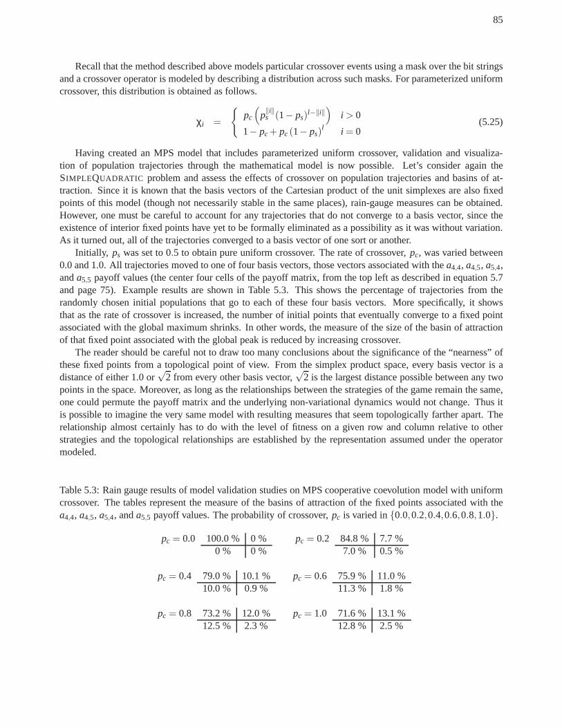
85

Recall that the method described above models particular crossover events using a mask over the bit stringsand a crossover operator is modeled by describing a distribution across such masks. For parameterized uniformcrossover, this distribution is obtained as follows.

χi =

pc

(

p‖i‖s (1− ps)

l−‖i‖)

i > 0

1− pc+ pc (1− ps)l i = 0

(5.25)

Having created an MPS model that includes parameterized uniform crossover, validation and visualiza-tion of population trajectories through the mathematical model is now possible. Let’s consider again theSIMPLEQUADRATIC problem and assess the effects of crossover on population trajectories and basins of at-traction. Since it is known that the basis vectors of the Cartesian product of the unit simplexes are also fixedpoints of this model (though not necessarily stable in the same places), rain-gauge measures can be obtained.However, one must be careful to account for any trajectoriesthat do not converge to a basis vector, since theexistence of interior fixed points have yet to be formally eliminated as a possibility as it was without variation.As it turned out, all of the trajectories converged to a basisvector of one sort or another.

Initially, ps was set to 0.5 to obtain pure uniform crossover. The rate of crossover,pc, was varied between0.0 and 1.0. All trajectories moved to one of four basis vectors, those vectors associated with thea4,4, a4,5, a5,4,anda5,5 payoff values (the center four cells of the payoff matrix, from the top left as described in equation 5.7and page 75). Example results are shown in Table 5.3. This shows the percentage of trajectories from therandomly chosen initial populations that go to each of thesefour basis vectors. More specifically, it showsthat as the rate of crossover is increased, the number of initial points that eventually converge to a fixed pointassociated with the global maximum shrinks. In other words,the measure of the size of the basin of attractionof that fixed point associated with the global peak is reducedby increasing crossover.

The reader should be careful not to draw too many conclusionsabout the significance of the “nearness” ofthese fixed points from a topological point of view. From the simplex product space, every basis vector is adistance of either 1.0 or

√2 from every other basis vector,

√2 is the largest distance possible between any two

points in the space. Moreover, as long as the relationships between the strategies of the game remain the same,one could permute the payoff matrix and the underlying non-variational dynamics would not change. Thus itis possible to imagine the very same model with resulting measures that seem topologically farther apart. Therelationship almost certainly has to do with the level of fitness on a given row and column relative to otherstrategies and the topological relationships are established by the representation assumed under the operatormodeled.

Table 5.3: Rain gauge results of model validation studies onMPS cooperative coevolution model with uniformcrossover. The tables represent the measure of the basins ofattraction of the fixed points associated with thea4,4, a4,5, a5,4, anda5,5 payoff values. The probability of crossover,pc is varied in0.0,0.2,0.4,0.6,0.8,1.0.

pc = 0.0 100.0 % 0 %0 % 0 %

pc = 0.2 84.8 % 7.7 %7.0 % 0.5 %

pc = 0.4 79.0 % 10.1 %10.0 % 0.9 %

pc = 0.6 75.9 % 11.0 %11.3 % 1.8 %

pc = 0.8 73.2 % 12.0 %12.5 % 2.3 %

pc = 1.0 71.6 % 13.1 %12.8 % 2.5 %

86

I also looked at parameterized uniform crossover whenps = 0.2 andpc = 1.0. The results for this showedthat the(4,4) basin captured roughly 62.6% of the trajectories, while the(4,5), (5,4), and(5,5) basins captured16.2%, 17.0% and 4.2% of the trajectories, respectively. Again, all trajectories found their way to one of thesefour basis vectors.

These are interesting results. They suggests that it is possible that previously unstable basis vectorfixed points become stable attractors under crossover. In a sense, crossover seems to “distract” trajecto-ries from always converging to the basis vector associated with the maximum value. To get a sense forwhy this might be, let’s look again at the 2D takeover plots shown in Figure 5.9 on page 87. In this case,pc ∈ 0.00,0.05,0.15,0.15,0.20,0.25.

There seems to be some kind of stretching transformation on the outer corners of the product simplex goingon as a result of crossover. As the rate of crossover increases, the trajectories are pushed away from the centerand move toward the edges at a much faster rate. In some cases these trajectories are drawn to basis vectorfixed points (homogeneous populations) not associated withthe global optimum. This behavior is observedin CCEA applications as well where one population convergesmuch faster than the other and reduces thedimensionality of the search by collapsing the space in which trajectories can pass to a face of the Cartesianproduct simplex. This corresponds to a reduction of the space to the unit simplex for the second population,still evolving population.

This is most likely explained by the accelerating effect crossover can have on population convergence(Menon 2002; Rabani, Rabinovich, and Sinclair 1998). This acceleration is applied asymmetrically, since theinitial conditions of the populations are almost certainlyasymmetric. To test this hypothesis, I ran an additionalexperiment in which all initial points for~x were chosen uniformly at random from the unit simplex, and allinitial points for~y were set symmetrically,∀i (~y)i = (~x)i, where(~x)i is the ith initial point. Although not alltrajectories converge to proper basis vector (the corner associated with the maximum value),noneconvergedsooner in one population than in the other. Figure 5.10 illustrates these results for different values ofpc.

Bit-flip Mutation

In a similar fashion, the mixing matrix M for the bit-flip mutation operator can be constructed. In this case,the diagonal elements ofM cannot be basis vectors as long aspm 6= 0 andpm 6= 1 since a population that iscompletely converged cannot remain so after mutation (in aninfinite population model). Therefore it is fair toconclude that the basis vectors are no longer fixed points under mutation.

Modeling bit-flip mutation is much simpler than modeling crossover, though analysis is much more difficult.Again a mask is used to apply a specific mutation event and the distribution of mutation masks models theoperator as a whole. With bit-flip mutation this is determined using a simple binomial distribution

µi = p‖i‖m (1− pm)l−‖i‖ (5.26)

wherepm represents the independent probability that a bit in a givenposition will be flipped. A careful reviewof the mixing formula will confirm that as long aspm 6= 0 andpm 6= 1, the diagonal of any valid permutation ofthe mixing matrix cannot be a basis vector. This makes sense:a population that is completely converged cannotremain so after mutation.

Unfortunately, this means that rain gauge measures of the type I used so far are not practical. Instead, Ican measure the distance of the point to the basis vector associated with the maximum payoff value. I rantrajectory studies withpm set to a variety of values. The result was that all the trajectories converged very closeto the same fixed point in all cases for a givenpm value, all 5000 initial conditions mapped to the same interiorpoint within an error radius of 10−4. Nevertheless, this point moved into the interior of the simplex product asmutation was increased. Figure 5.11 shows the 2D takeover plots for a few of these runs. The reader shouldnote that the distortions of the trajectories due to mutation are different than those produced by crossover.

This behavior matches intuition, as well as known results for the simple GA. As mutation is increased, thelimiting behavior is characterized as a distribution of population states that spread out away from the peak into

87

0.0

0.4

0.8

++++++++++++++++++++x

+

+++++++++++++++++++x

+

+++++++++++++++++++x

+

+++++++++++++++++++x

+

+++++++++++++++++++x+ +++++++++++++++++++x

+

+++++++++++++++++++x

+

+

++++++++++++++++++x++++++++++++++++++++x

+

+

++++++++++++++++++x+

+++++++++++++++++++x

+

+++++++++++++++++++x+ + ++++++++++++++++++x

+

+++++++++++++++++++x

+

+++++++++++++++++++x ++++++++++++++++++++x

+

+++++++++++++++++++x+

+++++++++++++++++++x

+

+++++++++++++++++++x

+

+ ++++++++++++++++++x+ +++++++++++++++++++x

+

+++++++++++++++++++x

+

+++++++++++++++++++x++++++++++++++++++++x

+

+++++++++++++++++++x+

+++++++++++++++++++x+

+++++++++++++++++++x+ +++++++++++++++++++x++++++++++++++++++++x

+

+++++++++++++++++++x0.

00.

40.

8

++++++++++++++++++++x

+

+++++++++++++++++++x+

+ ++++++++++++++++++x

+

+++++++++++++++++++x

+

+++++++++++++++++++x + +++++++++++++++++++x

+ +++++++++++++++++++x

+

+++++++++++++++++++x++++++++++++++++++++x

+

+++++++++++++++++++x+

+++++++++++++++++++x+

+++++++++++++++++++x+ +++++++++++++++++++x++++++++++++++++++++x

+

+++++++++++++++++++x + +++++++++++++++++++x

+

+++++++++++++++++++x++++++++++++++++++++x

+

+++++++++++++++++++x

+

+++++++++++++++++++x + +++++++++++++++++++x

+ +++++++++++++++++++x

+

+++++++++++++++++++x++++++++++++++++++++x

+

+++++++++++++++++++x+

+++++++++++++++++++x+

+++++++++++++++++++x+ +++++++++++++++++++x++++++++++++++++++++x

++++++++++++++++++++x

0.0 0.2 0.4 0.6 0.8 1.0

0.0

0.4

0.8

+ +++++++++++++++++++x

+

+++++++++++++++++++x++++++++++++++++++++x

++++++++++++++++++++x

+

+++++++++++++++++++x + +++++++++++++++++++x

+ +++++++++++++++++++x

+

+++++++++++++++++++x++++++++++++++++++++x+

+++++++++++++++++++x+

+++++++++++++++++++x+

+++++++++++++++++++x+ +++++++++++++++++++x++++++++++++++++++++x

++++++++++++++++++++x

0.0 0.2 0.4 0.6 0.8 1.0

+

+++++++++++++++++++x

+ +++++++++++++++++++x

+

+++++++++++++++++++x

+ +++++++++++++++++++x

++++++++++++++++++++x

+ +++++++++++++++++++x

+

+++++++++++++++++++x

+

+++++++++++++++++++x+

+++++++++++++++++++x

++++++++++++++++++++x

+

+++++++++++++++++++x++++++++++++++++++++x

+

+++++++++++++++++++x+

+++++++++++++++++++x++++++++++++++++++++x

Figure 5.9: 2D takeover plots for MPS trajectories in with uniform crossover. Reading from the left to the right,top to bottompc = 0.00,0.05,0.10,0.15,0.20,0.25.

88

0.0

0.4

0.8 +

+++++++++++++++++++x

+

+++++++++++++++++++x

+

+++++++++++++++++++x++++++++++++++++++++x

+

+++++++++++++++++++x+

+++++++++++++++++++x+

+++++++++++++++++++x

+

+

++++++++++++++++++x++++++++++++++++++++x

+

+++++++++++++++++++x+

+++++++++++++++++++x+

+++++++++++++++++++x

+

+

++++++++++++++++++x++++++++++++++++++++x+

+++++++++++++++++++x+

+++++++++++++++++++x+

+++++++++++++++++++x

+

+++++++++++++++++++x++++++++++++++++++++x

+

+

++++++++++++++++++x+

+++++++++++++++++++x+

+++++++++++++++++++x

+

+++++++++++++++++++x++++++++++++++++++++x

+

+++++++++++++++++++x++++++++++++++++++++x+

+++++++++++++++++++x

+

+++++++++++++++++++x++++++++++++++++++++x+

+++++++++++++++++++x0.

00.

40.

8 ++++++++++++++++++++x

++++++++++++++++++++x

+

+++++++++++++++++++x++++++++++++++++++++x

++++++++++++++++++++x

++++++++++++++++++++x

++++++++++++++++++++x

+

+++++++++++++++++++x++++++++++++++++++++x

+

+++++++++++++++++++x++++++++++++++++++++x+

+++++++++++++++++++x

+

+++++++++++++++++++x++++++++++++++++++++x+

+++++++++++++++++++x+

+++++++++++++++++++x+

+++++++++++++++++++x

++++++++++++++++++++x

++++++++++++++++++++x

++++++++++++++++++++x

++++++++++++++++++++x

++++++++++++++++++++x

+

+++++++++++++++++++x++++++++++++++++++++x

+

+++++++++++++++++++x++++++++++++++++++++x+

+++++++++++++++++++x

+

+++++++++++++++++++x++++++++++++++++++++x+

+++++++++++++++++++x

0.0 0.2 0.4 0.6 0.8 1.0

0.0

0.4

0.8 +

+++++++++++++++++++x+

+++++++++++++++++++x

++++++++++++++++++++x

++++++++++++++++++++x

++++++++++++++++++++x

+

+++++++++++++++++++x+

+++++++++++++++++++x+

+++++++++++++++++++x++++++++++++++++++++x+

+++++++++++++++++++x++++++++++++++++++++x+

+++++++++++++++++++x

+

+++++++++++++++++++x++++++++++++++++++++x+

+++++++++++++++++++x

0.0 0.2 0.4 0.6 0.8 1.0

+

+++++++++++++++++++x+

+++++++++++++++++++x

++++++++++++++++++++x

++++++++++++++++++++x

++++++++++++++++++++x

+

+++++++++++++++++++x+

+++++++++++++++++++x+

+++++++++++++++++++x++++++++++++++++++++x+

+++++++++++++++++++x++++++++++++++++++++x+

+++++++++++++++++++x+

+++++++++++++++++++x++++++++++++++++++++x+

+++++++++++++++++++x

Figure 5.10: 2D takeover plots for MPS trajectories in with uniform crossover with symmetric initial conditions.Reading from the left to the right, top to bottompc = 0.00,0.05,0.10,0.15,0.20,0.25.

89

0.0

0.4

0.8

++++++++++++++++++++x

+

+++++++++++++++++++x

+

+++++++++++++++++++x

+

+++++++++++++++++++x

+

+++++++++++++++++++x+ +++++++++++++++++++x

+

+++++++++++++++++++x

+

+

++++++++++++++++++x++++++++++++++++++++x

+

+

++++++++++++++++++x+

+++++++++++++++++++x

+

+++++++++++++++++++x+ + ++++++++++++++++++x

+

+++++++++++++++++++x

+

+++++++++++++++++++x+

+++++++++++++++++++x

+

+++++++++++++++++++x

++++++++++++++++++++x

+

+++++++++++++++++++x

+

+++++++++++++++++++x+ +++++++++++++++++++x

+

+++++++++++++++++++x

+

+++++++++++++++++++x++++++++++++++++++++x

+

+++++++++++++++++++x+

+++++++++++++++++++x

++++++++++++++++++++x+ +++++++++++++++++++x

++++++++++++++++++++x

+

+++++++++++++++++++x0.

00.

40.

8 + +++++++++++++++++++x

+

+++++++++++++++++++x+

+++++++++++++++++++x

+

+++++++++++++++++++x+

+++++++++++++++++++x+ +++++++++++++++++++x

+

+++++++++++++++++++x

+

+++++++++++++++++++x++++++++++++++++++++x

++++++++++++++++++++x++++++++++++++++++++x

++++++++++++++++++++x+ +++++++++++++++++++x++++++++++++++++++++x

++++++++++++++++++++x

++++++++++++++++++++x++++++++++++++++++++x+ +++++++++++++++++++x++++++++++++++++++++x+ +++++++++++++++++++x++++++++++++++++++++x

++++++++++++++++++++x

++++++++++++++++++++x++++++++++++++++++++x++++++++++++++++++++x++++++++++++++++++++x++++++++++++++++++++x++++++++++++++++++++x++++++++++++++++++++x++++++++++++++++++++x

0.0 0.2 0.4 0.6 0.8 1.0

0.0

0.4

0.8


0.0 0.2 0.4 0.6 0.8 1.0


Figure 5.11: 2D takeover plots for MPS trajectories in with bit-flip mutation. Reading from the left to the right,top to bottompm = 0.00,0.001,0.005,0.01,0.05,0.1.

90

the rest of the fitness landscape. However, notice that the destabilizing effects of crossover do not seem to occurin the case of mutation.

Mutation and Crossover

Validating and visualizing the effects of MPS models with both crossover and mutation (pc ∈ 0.0,0.1,0.2and pm ∈ 0.000,0.005,0.05) is now a straightforward exercise in producing a combined mixing matrix. Itis clear that the basis vectors are no longer fixed points. What is unclear is whether the combination of bothoperators will amplify the trajectory distortions produced individually, diminish them, or produce some othereffect.

0.0

0.4

0.8

++++++++++++++++++++x

+

+++++++++++++++++++x

+

+++++++++++++++++++x

+

+++++++++++++++++++x

+

+++++++++++++++++++x+ +++++++++++++++++++x

+

+++++++++++++++++++x

+

+

++++++++++++++++++x++++++++++++++++++++x

+

+++++++++++++++++++x

++++++++++++++++++++x

+

+++++++++++++++++++x+ + ++++++++++++++++++x++++++++++++++++++++x

+

+++++++++++++++++++x

++++++++++++++++++++x

++++++++++++++++++++x+ +++++++++++++++++++x

+

+++++++++++++++++++x+

+++++++++++++++++++x++++++++++++++++++++x

+

+++++++++++++++++++x

+

+++++++++++++++++++x++++++++++++++++++++x+

+++++++++++++++++++x++++++++++++++++++++x++++++++++++++++++++x+ +++++++++++++++++++x++++++++++++++++++++x

++++++++++++++++++++x


0.0

0.4

0.8

+ +++++++++++++++++++x

+

+++++++++++++++++++x+

+ ++++++++++++++++++x

+

+++++++++++++++++++x

+

+++++++++++++++++++x + +++++++++++++++++++x

+ +++++++++++++++++++x

+

+++++++++++++++++++x++++++++++++++++++++x

+

+++++++++++++++++++x++++++++++++++++++++x

++++++++++++++++++++x+ +++++++++++++++++++x

++++++++++++++++++++x

+

+++++++++++++++++++x

++++++++++++++++++++x++++++++++++++++++++x+ +++++++++++++++++++x++++++++++++++++++++x+

+++++++++++++++++++x ++++++++++++++++++++x

++++++++++++++++++++x

++++++++++++++++++++x++++++++++++++++++++x++++++++++++++++++++x++++++++++++++++++++x++++++++++++++++++++x+ +++++++++++++++++++x++++++++++++++++++++x

+

+++++++++++++++++++x


0.0 0.4 0.8

0.0

0.4

0.8

+ +++++++++++++++++++x

+

+++++++++++++++++++x++++++++++++++++++++x

++++++++++++++++++++x

+

+++++++++++++++++++x + +++++++++++++++++++x

+ +++++++++++++++++++x

+

+++++++++++++++++++x++++++++++++++++++++x+

+++++++++++++++++++x++++++++++++++++++++x

++++++++++++++++++++x+ +++++++++++++++++++x

++++++++++++++++++++x

++++++++++++++++++++x

0.0 0.4 0.8

++++++++++++++++++++x++++++++++++++++++++x++++++++++++++++++++x ++++++++++++++++++++x++++++++++++++++++++x + +++++++++++++++++++x

++++++++++++++++++++x

++++++++++++++++++++x++++++++++++++++++++x++++++++++++++++++++x++++++++++++++++++++x++++++++++++++++++++x++++++++++++++++++++x++++++++++++++++++++x

++++++++++++++++++++x

0.0 0.4 0.8


Figure 5.12: 2D takeover plots for MPS trajectories in with bit-flip mutation and parameterized uniformcrossover. Reading from the left to rightpc ∈ 0.0,0.1,0.2, from top top bottompm ∈ 0.000,0.005,0.05.

91

Figure 5.12 on page 90 shows six combinations of the model. Interestingly, the result of combining thevariation operators is additive in a sense. In these studies, trajectories fall towards the basis vectors associatedwith the center four payoff values as they did under crossover alone. The bottom two graphs in figure 5.12shows a projected version of this effect. However, observing the right two graphs, the limit point is pulled intothe interior of the simplex product space due to mutation.

5.3.3 Alternative Mixing Models

One reasonable complaint about the traditional EGT model isits supposition of complete mixing. Real CCEAsrarely evaluate an individual by pairing it with all possible collaborators. Indeed, as I discussed in the previouschapter, many CCEAs use a very few, fixed number of collaborators.

Still, there is no reason that the model cannot be modified to consider alternative mixing models, thoughwhat kind of quality of analysis is possible with them is as yet unclear. I will discuss two very simple partialmixing models as a proof of concept. These two methods consider both the idea of biasing the collaborationsampling process an the idea of enforcing a fixed size to the sample: complete-weighted collaboration andc-random collaboration.

Complete-Weighted Collaboration

The idea behind complete-weighted collaboration is simple: individuals are paired with all possible individualsfrom the alternate population, but the degree of contribution to the fitness assessment process is weighted byfitness result of the individual in the previous generation.Implementing this approach requires modificationsof the original replicator equations that consider a time variable, t. Given thatt := 1 is defined in the initialconditions, then the system can be described by the following equations.

ui(t) = (A~y)i ·wi(t −1) (5.27)

wi(t) =(

AT~x)

i ·ui(t −1) (5.28)

x′i =( ui

~x·~u)

xi (5.29)

y′i =

(

wi

~y·~w

)

yi (5.30)

ui(0) = 1 ∀i ∈ 1, . . . , r (5.31)

wi(0) = 1 ∀i ∈ 1, . . . , r (5.32)

c-Random Collaboration

Constructing a partial mixing model that uses only a finite number of collaborators in an infinite population issomewhat more difficult. I begin by noting that the original replicator equations (Eq. 5.3–5.6) can be used asis for a single-random collaborator. In such a case, the vector components in the first two utility assessmentequations refer to the probability that a particular collaborator is picked. Since the population is infinite, andthe collaborator is picked uniformly at random, the result of the same set of equations for complete mixing canbe see as a model for theexpectedoutcome when one selects a single random collaborator.

To c such selections, return to the idea of using masks. Define a masking bit string of lengthn and aparticular string indicating the outcome of a particular collaboration event in terms of which genotypes willserve as collaborator. Given a distribution of masks,C, the augmented replicator equations follow.

92

~u =∑

j∈Ω

Cj ·A(diag( j) ·~y) (5.33)

~w =∑

j∈Ω

Cj ·AT (diag( j) ·~x) (5.34)

x′i =( ui

~x·~u)

xi (5.35)

y′i =

(

wi

~y·~w

)

yi (5.36)

The function diag( j) considers the bit stringj of lengthn and constructs ann×n matrix such that the bit stringrepresents the diagonal of the matrix and all other values are zero.

This is a somewhat general mechanism that allows for many kinds of collaboration methods by detailingdifferent kinds of mask distributions; however, I will concern myself with using only a fixed number ofc ran-domly selected collaborators. The result is again theexpectedoutcome of the particular collaboration samplingmethod. For a fixed number of collaborators, the distribution of collaborator masks can be computed as follows.

Cj =

c!(n−c))!n! if ‖ j‖ = c0 otherwise

(5.37)

This model still suggests an averaging of multiple functionevaluations is used for credit assignment pur-poses (i.e., thehedgemethod). There are obvious augmentations that can be applied to construct a model thatassigns fitness using the maximum possible payoff of the collaborators, but they have the distinct analytic dis-advantage of being discontinuous. Additionally, the two suggestions here may be naturally combined with oneanother to produced a biased, finite sample expected outcomemodel for collaboration.

5.4 Empirical Examples

Some empirical examples are helpful since the theoretical models I’ve provided differ in several significantways from real CCEAs applied to static optimization problems. One difference is that populations are quiteobviously not infinite in size. Another difference is that collaboration methods do not really resemble completemixing, in general.

However, despite its limitations, this dynamical systems model has provided some concrete answers to rel-atively philosophical questions, as well as some insight into what some coevolution pathologies might actuallylook like. Moreover, the infinite population model can be seen as an expectation for the behavior of finitepopulation models. With this, we have an answer to the fundamental question: one cannotexpectthese sys-tems to gravitate toward optimal collaborations, even in the ideal case where stochastic effects are minimal, ornon-existent. This corresponds exactly with the relative overgeneralization pathology discussed above.

Moreover, visualization of the model has revealed insight into how asymmetries in initial conditions andproblem characteristics can exacerbate asymmetries in rates of evolutionary changes between populations. Assuch, we canseeloss of gradient actually occur.

Nevertheless, a bridge between the abstract model in which these pathologies gained clarity, and real al-gorithms in which they are manifested is necessary. Indeed,now that a better understanding of these twodifficulties has been achieved, it is a simple matter to create examples that illustrate them in more realistic set-tings. This section provides two such examples. In the first case, the pathology of relative overgeneralization isdemonstrated using the MAX OFTWOQUADRATICS problem already defined, while in the second case a variantof this problem is used to show loss of gradient. Such examples will make tangible connections between theoryand practice.

93

In both cases I used a two population, generational cooperative coevolutionary algorithm with fitness pro-portionate selection. Collaboration involved all membersof the cooperating population, and the mean result(hedge) was assigned as fitness. This is consistent with the complete mixing idea in the formal model. The pre-vious generation of the alternate population was used to assess fitness for individuals (i.e., the parallel updatingmechanism). Each population contained 100 individuals. Individuals are encoded using a binary representation(64 bits), and the genetic operators were bit-flip mutation (pm = 1/64) and parameterized uniform crossover(parameter values vary between experiments, see subsections below). In all, the real CCEA was quite similarto the theoretical model.

Comparisons to a traditional EA are made in both examples. The EA in question is as analogous to theCCEA with which it is compared as is possible. The populationcontained 200 individuals, and individualswere bit strings of length 128. The same genetic operators were applied, but the mutation rate was set at 1/128.Again, fitness proportionate selection was used.

5.4.1 Relative Overgeneralization

In order to demonstrate the relative overgeneralization pathology in an empirical setting, the algorithms de-scribed above were applied to the MAX OFTWOQUADRATICS problems defined the parameters listed in Ta-ble 5.4.1. Each algorithm was run 50 independent times against each of these 8 problems for 100,000 functionevaluations per trial. Crossover was not used in these cases(pc = 0.0).

Table 5.4: This table describes the parameter settings usedfor the MAX OFTWOQUADRATICS function in theempirical experiments.

Parameter Value(s)k1 150k2 140s1 2,4,8,16,32,64,128,256s2 1

(x1, y1) (8,1)(x2, y2) (1,8)

Two graphs were produced to illustrate the results, shown onpage 94. The first (on top) shows the averagesand confidence intervals for the final best-ever fitness values obtained for each group, while the second moreinformatively shows the ratio of those values that exceed 140. The purpose of this second plot is to illustratethe ratio trials that escaped the suboptimal peak.

Pairwiset-tests with Bonferoni adjustments show that the best-ever fitness values obtained by the CCEAwere statistically inferior to the comparable EA for all groups. In both cases, however, the best-ever resultunsurprisingly declines as the value ofs1 increases. From the ratios we see what differs between thesetwoalgorithms: in the CCEA case, an increasing number of trialsare being mislead and converge to the suboptimalpeak, rather than the global optimum. Conversely, the EA does not seem to suffer from this problem as deeply.While average best-ever fitness values are clearly affectedby the parameter change, no such drastic increase inthe local convergence is observed at very high values ofs1, s1 = 256 in particular (wherenoneof the CCEAtrials escape local convergence).

5.4.2 Loss of Gradient

The loss of gradient challenge is more difficult to illustrate in realistic settings. To try to do so, let’s considerthe algorithms described above were applied to a modified form of the MAX OFTWOQUADRATICS problemclass, called ASYMMETRICTWOQUADRATICS. In this case, the peak widths can be varied independently to

94

0 50 100 150 200 250

130

135

140

145

150

CCEAEA

0 50 100 150 200 250

0.0

0.2

0.4

0.6

0.8

1.0

Figure 5.13: CCEA and EA empirical results on MAX OFTWOQUADRATICS ass1 is increased. Thex-axis forboth graphs shows the value for thes1 parameter. In the top graph, they-axis displays final best-ever fitnessresults. The points are mean values of 50 trials, while the wings are 95% confidence intervals. The bottomgraph shows the ratio of the 50 trials in which the best-ever value exceeds 140.0.

adjust asymmetric conditions in the landscape between the two arguments. The function is defined below. Inthe experimental groups here, all problem class parametersare defined as they are above, save for the followingdifferences. Thesx2 andsy2 parameters were both set to 1, and thesx1 parameter was held fixed at 4. Thesy1

parameter, however, was varied using the values2,4,8,16,32,64,128,256.

Definition 31. Given constant values defining the two peaks: k1 and k2 to define the peak heights. Asymmetricpeak widths are defined by the parameters sx1, sx2, sy1, and sy2. Again, the points(x1, y1) and(x2, y2)define the locations of the peaks. The functionASYMMETRICTWOQUADRATICS : N×N → R

is defined by

quad1(x,y) = k1−[

sx1 · (x1−x)2 +sy1 · (y1−y)2]

quad2(x,y) = k2−[

sx2 · (x2−x)2 +sy2 · (y2−y)2]

ASYMMETRICTWOQUADRATICS(x,y) = max(quad1,quad2)

Again, each algorithm was run 50 independent times against each of these 8 problems for 100,000 functionevaluations apiece. This time crossover was applied (pc = 1.0, ps = 0.5) in order to exaggerate the effects ofloss of gradient. The first figure below again shows the best-ever fitness values and convergence ratios for eachof the 8 groups with crossover.

95

0 50 100 150 200 250

130

135

140

145

150

CCEAEA

0 50 100 150 200 250

0.0

0.2

0.4

0.6

0.8

1.0

Figure 5.14: CCEA and EA empirical results on ASYMMETRICTWOQUADRATICS without crossover assx1 isincreased. Thex-axis for both graphs shows the value for thesx1 parameter. They-axis displays final best-everfitness results. The points are mean values of 50 trials, while the wings are 95% confidence intervals.

Statistically speaking, there is no doubt that the parameter value has an effect on CCEA performance, muchas it did in the previous section with the MAX OFTWOQUADRATICS problem. However, with this visualizationit is nearly impossible to see what exactly is happening in terms of gradient loss. To see this, I tracked thestandard deviation in fitness values for each of the two populations. The resulting standard deviations fromthe final generation of the two populations can be visualizedas a scatter plot of the 50 order pairs considered.The result (shown in Figure 5.15 on page 96) shows that assx1 increases, the it becomes harder and harder forthe algorithm to maintain a consistent standard deviation between the two populations. To help see this effect,I’ve provided a linear regression of the scatter plot. This line “tips” as the landscape becomes more skewed,showing a greater tendency for the populations to attain different levels of diversity. Points begin to line up inthe scatter plots, suggesting that when the CCEA terminated, it was typical for one population to be much morediverse than the other.

These graphs indicate loss of gradient. Adding asymmetry causes population diversity between the twopopulations to become increasingly more asymmetric, the result of which is shown in Figure 5.14. Further, theconvergence problems (as illustrated by the ratio graph) seem even more disparate between the EA and CCEAthan they did in the MAX OFTWOQUADRATICS case. Indeed, loss of gradient can be among the most seriousstumbling blocks for cooperative coevolution.

96

9010

011

012

013

014

0

80 100 120 140

8090

110

130

70 80 90 100 110 120 130 140

Figure 5.15: These four graphs show co-plotted standard deviations of population fitness at the end of the run.The line is a linear regression fit of the scatter plot. The groups shown appear left to right, top to bottom assx1 = 4, 16, 64, and 256, respectively.

Chapter 6

New Views of CCEAs

In the previous chapter, I showed that the cooperative coevolutionary algorithm may not be particularly well-suited (in general) to static optimization problems that are straightforwardly encoded. In some sense, this can beseen as the main message of this dissertation. It addresses the fundamental question posed in the introduction:“What does this tooldo?”. Put more specifically, I asked “Do CCEAs optimize?”. The answer here is: the toolis not a static optimizer of ideal collaboration (i.e., the specific collaboration that results in the optimal fitness),but rather it seems to be an adaptive optimizer of the joint distribution of rewards described by collaborationspace.

I believe this knowledge is helpful and useful to practitioners. The general contribution of this is to illustrateplainly to those studying cooperative coevolutionary algorithms that anew viewof what CCEAs do, and howthey work is imperative if we are to make progress in applyingthem successfully. This chapter attempts to makemy main message clearer by offering several specific high level suggestions of such new views. These viewsstem from answers to the question, “If one should not apply the simple CCEAs described here to straightforwardstatic optimization problems, what is to be done with them?”

There are several things this thesis doesnot say. First, it does not suggest that CCEAscannotbe applied tostatic optimization problems, nor does it even suggest thatsuch applications will never be successful. Second,it does not really directly answer the most basic form of the fundamental question since it is not at all clearwhat the application-oriented meaning of an “adaptive optimizer of the joint distribution of rewards describedby collaboration space” is. These are fair observations, and I will respond to both of these points at the end ofthe chapter.

This chapter provides the community with some high level advice for the direction that future researchersmight take, given the message established here. I take the very simple tack that if the CCEA should notnecessarily be expected to perform static optimization tasks, something should be done to either change theexisting algorithms or how, and to what, one applies them. With this view in mind, the chapter offers threesimple high level suggestions for how one might improve the results of the algorithm by either altering thealgorithm itself or by applying it more appropriately. The first section addresses the difficulties caused bythe algorithms’ propensity towards robust resting balanceby describing a simple, but extensible method forbiasing the algorithm toward a preference for ideal collaborations. Maintenance of the adaptive evolutionarybalance is the subject of the second section, which describes an attempt reduce the problems of gradient loss byaugmenting a CCEA with a means of balancing the rates of evolutionary change in the respective populations.The third section provides a short philosophical discussion about the kinds of problems for which traditionalcooperative coevolutionary algorithms may be more appropriate. In the final section I will provide a briefconclusion about the main theme of the dissertation.

6.1 Biasing Towards Static Optimization

Part of the difficulty the CCEAs I’ve discussed thus far face when applied to static optimization problem is thefact that an individual’s fitness is commonly assessed only by a subset of the potential interaction space. That is,it is assessed (typically) based on how well it performs withimmediate individuals from the other populations.

97

98

In a very literal sense, this is taking aprojectionof the total interaction space. Such a projection, generated bysampling the space using the collaborating populations, may or may not provide the search with adequate orappropriate information to lead it towards the ideal collaboration.

This difficulty speaks to the first form of balance discussed earlier, the one most stressed by this dissertation:the tendency towardrobust resting balance. That is CCEAs tend toward the resting balance of Nash equilibriaassociated with high joint distribution values in the payoff matrix, not toward optimal collaboration. Since formany very realistic problems such equilibria may be highly-suboptimal, this tendency can lead to one of thepathologies discussed in the previous section: relative overgeneralization.

To find optimal collaborations, the search process may need to be more aggressive than this: assessingfitness based more on thehighest-rewardinteractions between an individual and various members of the otherpopulation. Indeed, this is part of the spirit of the empirical ideas discussed in Chapter 4 with respect to the useof the optimistic credit assignment collaboration method,which tended to yield better results than when usingthe mean or minimum performance. This has the advantage of being more opportunistic, forming a projectionthat considers the basic intent of the optimization algorithm: find the ideal. But it is still a projection—and theinformation used to construct this projection is still limited to the current context.

The idea presented here is similar to this opportunistic approach, and bears a slight resemblance to the “Hallof Fame” concept introduced by Rosin and Belew (1997) for competitive coevolution. An individual’s fitnessmight be based on a combination of its immediate reward whileinteracting with individuals in the populationand an estimate for the reward it would have received had it interacted with its “ideal collaborators”. Moreover,the fraction of reward due to the immediate (as opposed to theideal) interaction might be adjusted during thecourse of the run. In this way, the projection that is formed during one part of the search is one that considers awider context that allows for more exploration of unseen parts of the space, or it may consider a more narrowscope at other times during the search.

This idea of an optimization biased CCEA can be justified in the following way. Recall that if an individual’sfitness is based on its immediate interaction with individuals from the other population, then~u = A~y and~w =AT~x, as described in equations 5.3 and 5.4. Now, let us consider afunction max(A) that returns a column vectorcorresponding to the maximum value of each row in matrixA. Now, if an individual’s fitness is based on itsmaximum possible performance in conjunction with any individual from the other population, then one maymodify equations 5.3 and 5.4 to be~u = max(A)T and~w = max

(

AT)T

.

In this modified system, the tendency to optimize performance is clear since the new fitness measure willresult in populations that converge to basis vectors associated with any unique maximal value in the payoffmatrix. At each iteration of the model, the fitness of each strategy will be its best possible fitness. If there is aunique maximum, that result will have the highest fitness, and so the proportion of the corresponding strategywill increase in the next step. The reason for this should be obvious: the problem has lost the dimension-ality added due to the nature of the interactions between thepopulations and has been reduced to a simpleevolutionary algorithm. Regardless of the content of the opposing population, the fitness measure for a givenstrategy is the same. As shown in Reeves and Rowe (2002, Vose (1999), an infinite population model of thisreduced evolutionary algorithm will converge to a unique global maximum. In fact, the algorithm is no longercoevolutionary in any real way.

Of course, this idyllic discussion has a major flaw: a real CCEA algorithm would not know the maximumpossible reward for a given individuala priori. To make use of any bias, this knowledge will have to estimatedusing some kind of learning mechanism. One approach is to usehistorical information during the run toapproximate the maximum possible collaborative fitness foran individual. However, if the approximation istoo large (or has too strong an effect on the overall fitness),and if it appears too early in the evolutionary run,then it can deform the search space to drive search trajectories into suboptimal parts of the space from whichthey cannot escape. On the other hand, if the approximation affects the fitness measurement very weakly, andtoo late in the run, then it may not be of much help, and the system will still gravitate towards balance. To bettersee this tradeoff, equations 5.3 and 5.4 may be again alteredsuch that a bias weight parameter,δ, is added

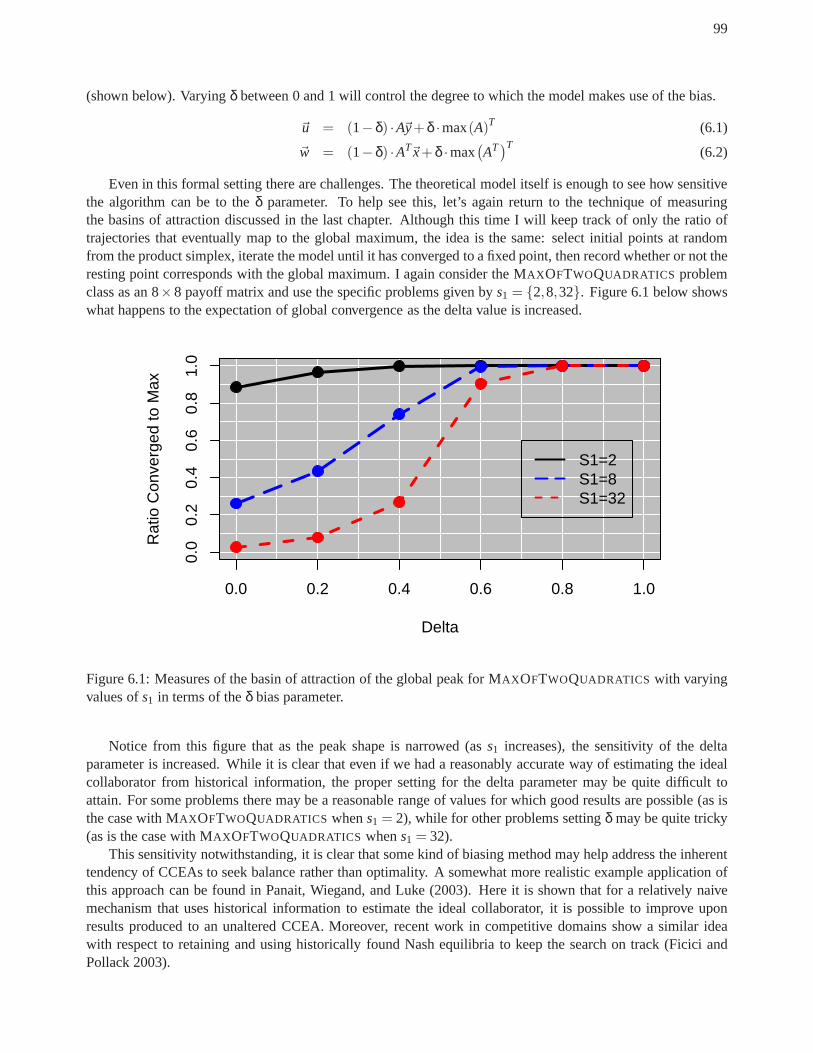
99

(shown below). Varyingδ between 0 and 1 will control the degree to which the model makes use of the bias.

~u = (1−δ) ·A~y+ δ ·max(A)T (6.1)

~w = (1−δ) ·AT~x+ δ ·max(

AT)T (6.2)

Even in this formal setting there are challenges. The theoretical model itself is enough to see how sensitivethe algorithm can be to theδ parameter. To help see this, let’s again return to the technique of measuringthe basins of attraction discussed in the last chapter. Although this time I will keep track of only the ratio oftrajectories that eventually map to the global maximum, theidea is the same: select initial points at randomfrom the product simplex, iterate the model until it has converged to a fixed point, then record whether or not theresting point corresponds with the global maximum. I again consider the MAX OFTWOQUADRATICS problemclass as an 8×8 payoff matrix and use the specific problems given bys1 = 2,8,32. Figure 6.1 below showswhat happens to the expectation of global convergence as thedelta value is increased.

0.0 0.2 0.4 0.6 0.8 1.0

0.0

0.2

0.4

0.6

0.8

1.0

Delta

Rat

io C

onve

rged

to M

ax

S1=2S1=8S1=32

Figure 6.1: Measures of the basin of attraction of the globalpeak for MAX OFTWOQUADRATICS with varyingvalues ofs1 in terms of theδ bias parameter.

Notice from this figure that as the peak shape is narrowed (ass1 increases), the sensitivity of the deltaparameter is increased. While it is clear that even if we had areasonably accurate way of estimating the idealcollaborator from historical information, the proper setting for the delta parameter may be quite difficult toattain. For some problems there may be a reasonable range of values for which good results are possible (as isthe case with MAX OFTWOQUADRATICS whens1 = 2), while for other problems settingδ may be quite tricky(as is the case with MAX OFTWOQUADRATICS whens1 = 32).

This sensitivity notwithstanding, it is clear that some kind of biasing method may help address the inherenttendency of CCEAs to seek balance rather than optimality. A somewhat more realistic example application ofthis approach can be found in Panait, Wiegand, and Luke (2003). Here it is shown that for a relatively naivemechanism that uses historical information to estimate theideal collaborator, it is possible to improve uponresults produced to an unaltered CCEA. Moreover, recent work in competitive domains show a similar ideawith respect to retaining and using historically found Nashequilibria to keep the search on track (Ficici andPollack 2003).

100

There are, of course, many open questions about how to apply such a method in a more realistic way;however, given the right estimation methods and parameter settings, biasing coevolution towards optimalitymight be one effective way of altering the basic cooperativecoevolutionary algorithm to more more gearedtowards the task of static optimization. For these reasons,it certainly merits further study.

6.2 Balancing Evolutionary Change

Like the previous section, this section attempts to resolvethe problem with CCEAs by correcting the algorithm.Indeed, both sections consider the ideas of balance, thoughdifferently. In the previous section, the idea wasto thwart the natural tendency of the CCEA toward robust resting balance by biasing the algorithm towardoptimal collaboration. This section, however, attempts toaddress the issue of dynamic balance by attemptingto preserve that balance.

As I described in Chapter 5, coevolutionary algorithms “progress” while remaining in a type of adaptivebalance. To lose that balance means that one or more populations will collapse to near homogeneity, and theremaining populations will lose some, or all, of their gradient for search. In the context of the applicationof these symmetric CCEAs on static optimization problems, it is clear that if one can keep the algorithmprogressing in terms of increased payoff values, the optimum will be reached (eventually). So how can this bedone?

Recall that the effects of variation (and possibly even stochastic selection) can exacerbate asymmetries inthe initial conditions and the problem itself, which can lead to the destabilization in the balance the the search.The result is often some form of loss of gradient. Is there a way to protect the dynamic balance of the search bydampening these effects?

One possible approach might be to localize the operators using some kind of spatial embedding (Sarma1998). For example, a two-population CCEA might be distributed on two, matched-up grids such that each gridpoint corresponds to an individual (e.g., see Figure 6.2). Selection is performed locally within some pre-definedneighborhood, and collaboration is similarly constrainedto the corresponding neighborhood in the matchedgrid. Indeed, such coevolutionary algorithms have been shown to work better than corresponding non-spatialCEAs for some, very specific problems (Pagie 1999). The reasoning behind their advantage has, until now, notbeen explained.

Figure 6.2: Example spatial distribution grids for a two-population CCEA

One reason might be that, transmission of information within a population is not only slowed and localized,but it is in some sensecapped. That is, there is a maximum computable rate at which information can diffuseacross the population, given the relationship of the local neighborhoods to the population itself (Sarma 1998).This means that the two populations might be way “locked” together in terms of their rate of change. Moreover,

101

asymmetries in the problem can be in some way countered (if they are known or suspecteda priori) by adjustingthe neighborhoods for collaborations relative to one another.

To test this idea, the following experiments were performed. A two-population CCEA was applied to theASYMMETRICTWOQUADRATICS static optimization problem class, save that the domain values were scaledbetween 1.0 and 8.0, as with the experiments discussed at theend of the previous chapter. The parameters toinstantiate the problems used here are shown in Table 6.2.

Table 6.1: Parameters for the MAX OFTWOQUADRATICS problem used in the spatial embedding experiments.

Parameter Valuek1 150k2 140sx1 2,4,8,16,32,64,128,256sx2 1sy1 4sy2 1

(x1, y1) (8,1)(x2, y2) (1,8)

I compare the CCEA results on the ASYMMETRICTWOQUADRATICS problem from the previous chapterto a spatial model where 49 members of each population are laid out in 7× 7 toroidal grids. A given gridposition refers, then, to two individuals: one in the first population and one in the second. Collaborationconsisted of using the 3×3 Moore neighborhood in the alternate population centered at the same position asthe individual being evaluated. The mean of these 9 values was used as the fitness value for the individual beingevaluated. Proportionate selection likewise used a 3×3 Moore neighborhood around the present individual inthe populations. This meant that the 9 individuals associated with a given position were used to construct aweighted distribution, a draw was taken from that distribution, and the winner was substituted into the givenposition in the next round. The positions were processed in random order (without replacement). Again,crossover was applied as it was before (pc = 1.0 andps = 0.5). The update mechanism was parallel.

Each group was run 50 times and the best result found during the search was preserved in each trial. Thebest-ever results, as well as the ratio of final generation best values exceeding 140, are shown in Figure 6.3. Thevalues for every group are far improved over the non-spatialresults shown on page 95. The best-ever resultsare statistically significant for all values ofsx1. Looking again at the scatter plots of the standard deviationsof the final generation of the runs (Figure 6.4 on page 103) provides with some clue as to why. Though atfirst it may appear that all of the regression lines are tippedin this case, there are two important things to note.First, the overall standard deviations are much lower than those shown on page 96. Second, the differencesbetween the relationships of standard deviations are much less pronounced between different values ofsx1.This suggests that increasing the value ofsx1, in effect skewing the problem more and more, had little impacton the relationship of the final generation’s population diversities.

Again, it is obvious that there are more questions about how to go about applying this method than there isadvice provided here. The point was not to demonstrate a particular method, but to underscore the idea that bypreserving the dynamic balance of the CCEA, better results might be obtained by reducing the risks associatedwith the problem of loss of gradient. Many other methods exist for accomplishing something similar.

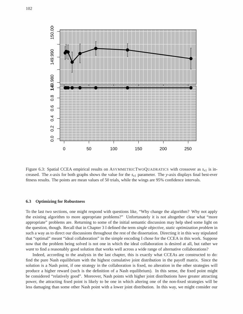
102

0 50 100 150 200 250

149.

980

149.

990

150.

000

0 50 100 150 200 250

0.0

0.2

0.4

0.6

0.8

1.0

Figure 6.3: Spatial CCEA empirical results on ASYMMETRICTWOQUADRATICS with crossover assx1 is in-creased. Thex-axis for both graphs shows the value for thesx1 parameter. They-axis displays final best-everfitness results. The points are mean values of 50 trials, while the wings are 95% confidence intervals.

6.3 Optimizing for Robustness

To the last two sections, one might respond with questions like, “Why change the algorithm? Why not applythe existing algorithm to more appropriate problems?” Unfortunately it is not altogether clear what “moreappropriate” problems are. Returning to some of the initialsemantic discussion may help shed some light onthe question, though. Recall that in Chapter 3 I defined the term single objective, static optimization probleminsuch a way as to direct our discussions throughout the rest ofthe dissertation. Directing it in this way stipulatedthat “optimal” meant “ideal collaboration” in the simple encoding I chose for the CCEA in this work. Supposenow that the problem being solved is not one in which the idealcollaboration is desired at all, but rather wewant to find a reasonably good solution that works well across a wide range of alternative collaborations?

Indeed, according to the analysis in the last chapter, this is exactly what CCEAs are constructed to do:find the pure Nash equilibrium with the highest cumulative joint distribution in the payoff matrix. Since thesolution is a Nash point, if one strategy in the collaboration is fixed, no alteration in the other strategies willproduce a higher reward (such is the definition of a Nash equilibrium). In this sense, the fixed point mightbe considered “relatively good”. Moreover, Nash points with higher joint distributions have greater attractingpower, the attracting fixed point is likely to be one in which altering one of the non-fixed strategies will beless damaging than some other Nash point with a lower joint distribution. In this way, we might consider our

103

02

46

810

12

2 4 6 8 10 12

24

68

3 4 5 6 7 8 9

Figure 6.4: These four graphs show co-plotted standard deviations of population fitness at the end of the run.The line is a linear regression fit of the scatter plot. The groups shown appear left to right, top to bottom assx1 = 4, 16, 64, and 256, respectively.

solutionrobust: it is relatively good and is susceptible to harm by minor changes in the alternate strategies thanother such points. Suppose, then, one is interested in optimizing for robustness, rather than ideal collaboration?

It is reasonable to consider such a viewpoint. Take, for example, the problem of learning behaviors formultiple, collaborating agents in some kind of stochastic domain. Presumably one is, on the one hand, lessinterested in the best possible solution than a satisfactory one and, on the other hand, more interested in solutionsthat are reasonably stable in the face of minor fluctuations in the team behaviors. In other words, it is usuallybetter to have a team that will still perform relatively wellwhen one or more members behaves differently thanone expects, than it is to have one which performs very well only if every member does exactly what it should.

Consider the MAX OFTWOQUADRATICS, s1 = 32 problem example again. For the sake of argument, let’ssuppose that this landscape describes the performance results of two, cooperating agents. If the object is to learngood, but robust behaviors, which peak is the “better” peak?The global peak has the disadvantage that anychange by either partner in their strategy could bring abouta rather dramatic loss of performance. In realisticmulti-agent settings, this could happen for a variety of reasons (e.g., a servo on the robot fails for some reason).The second, suboptimal peak offers a much more stable result.

104

6.4 Conclusions

The main message of this dissertation is a response to the fundamental question posed at its start: one shouldnot expect CCEAs (in general) to perform well on single objective, static optimization problems because dy-namically they are predisposed to achieving states of robust resting balance over those of ideal collaboration.Recall, though, that there are at least two important caveats mentioned above: I do not suggest that CCEAscannot be successfully applied to static optimization problems, nor do I offer a great deal of detailed adviceclarifying how they should be applied.

I will now look at these two issues in turn, suggesting futureresearch opportunities as I do so, as well asunderscoring the research contributions of this work. Afterward, I will suggest the less tangible methodologicalcontribution of this work.

6.4.1 Applying CCEAs to Static Optimization

Can CCEAs be applied successfully to static optimization problems, despite their internal dynamic tendencies?Of course they can be. In Chapter 4 I show clearly that CCEAs can perform competitively with more traditionalEAs on some kinds of problems. Moreover, the No Free Lunch theorem tells us that all algorithms perform (onaverage) the same against any problem set that is closed under permutation (Schumacher, Vose, and Whitley2001). Onecanapply CCEAs to such problems, and onecanexpect it to perform reasonably well at times.

Nevertheless, in the more specific situations where practitioners are interested in a subset of problems thathave certain, very reasonable and common properties, the use of CCEAs should be reconsidered. I have shownthat for very simple problems that contain some kinds of cross-population nonlinearities, the CCEA can havesome very pathological difficulties. Moreover, whatever the underlying relevant property that creates challengesfor these methods, it is something more complex than simply the existence of such epistatic connections. Thereare clearly certainkindsof nonlinear relationships between populations that create difficulties, and there areclearly other relationships at play as well. The existence of cross-population epistasis is neither a necessary norsufficient condition to raise the red flag of warning.

However, in spite of the challenges presented by these algorithms, there’s some hope that they can bemodified to be more suited for static optimization procedures. I suggested two such ways. In the first, thealgorithm might be explicitly biased toward ideal collaboration by considering historical information regardingthe interaction search space. In the second, I offered one method for how adaptive balance in the algorithmmight be preserved by harnessing the constraining effects of spatial embedding as a means of tying changes intwo populations together. Both ideas are only one of many ways to address their respective issues. I presentedthem as conceptual examples, not as specific rigid dictums for how to solve these cooperative coevolutionarydifficulties.

At this level of abstraction, these ideas contribute adviceto the future of the study of cooperative coevo-lutionary algorithms in a very real way: researchers shouldfocus on similar kinds of modifications to addressthese challenges, if they wish to continue to use these algorithms in such settings.

6.4.2 Adaptive optimization of robustness

So what do CCEAs really do? My answer is that they are adaptiveoptimizers of robustness or, more explicitly,they attempt to adaptively discover places in the search space with maximal joint distribution of rewards asdescribed by the collaboration space. It might be intimatedthat this is only an indirect answer to the fundamentalquestion since it is not necessarily clear exactly what thisstatement means. Moreover, while it is important toknow what CCEAsdo notdo, it is also important to know what theydo.

Research into the field of coevolutionary computation has been distracted by several misconceptions aboutthe algorithms themselves, and particularly about how theyfunction. To some extent, we must revisit investi-gations of CEAs in a more focussed light. The contributions provided here are more than simple disputation

105

because they inform researchers that we must step back and take a new look at the algorithms from a moreinformed perspective with respect to their function. What is needed is a new view of the CCEA in terms of theproblems it solves.

While the clarity of what the real-world implications of “adaptive optimization of robustness” may be indoubt, researchers who view CCEAs through this lens will be more successful at determining how CCEAs canbe best applied. If nothing else, future researchers of coevolutionary computation should consider this beforebeginning their research: make certain that the algorithm is solving the problem that is being encoded, and notsomething quite different than one might have expected.

6.4.3 A Methodological Framework

Perhaps a far less tangible contribution of this dissertation can be found in its methodological approach. Thereare two points in this matter that I would like to underscore.

On a general level, there is at least one classical methodological decision made by this research that isworth pointing out. I began with a question and addressed allanalysis and experimentation to that question,or subordinate instantiations of that question. Specifically, I began with a very broad question, and refinedit in different ways based on context. These refinements produced more specific questions that were moreresearchable. The process of starting broadly and refining to specific question is a framework that offers greatdeal in focussing research that has many angles,.

As an example, the “fundamental question” was just such a broad question. I outlined this at the start of thedocument and continually refined it in each context of my analysis. Moreover, I kept the question as simple aspossible. Indeed, I offer this suggestion for future research in coevolutionary computation: continue tobeginresearch with that fundamental question: “What do these algorithms really do?”

However, beyond the more obvious and classical methodological observations, I want to say a few wordsabout the analytical tools used in my research. There is a great deal of controversy and tension in the evolu-tionary computation field about the utility and informativeness of various theoretical ideas. Some believe thatdynamical systems approaches tell us very little about whatreal algorithms will do in terms of how long wecan expect to wait for “good” solutions, while others believe that they help us model and understand algorithmlimiting behaviors as they are in their most abstract and simplest form. Some believe that run time analysisis unhelpful because it can only answer questions about verysimple, unrealistic algorithms on very contrivedproblems, while others believe that they provide very specific and precise information about real algorithms(rather than models of algorithms). Even more extremely, some believe that no theoretical approach has so farproved helpful to practitioners, while others hold practitioners as irresponsible for poor empiricism born out ofa lack of fundamental understanding of the algorithms they use.

What is the truth? The truth is that one needn’t discard any ofthese tools, but recognizing their advantagesand limitations, one can apply many them in different ways.Many of these methods can help answersometypes questions, as long as the questions are properly posed. It may be difficult to understand how dynamicalsystems methods can be used to inform us of how long users mustwait for solutions, but it is not difficult tounderstand how they can inform us about whether not the algorithms are even attracted to those solutions in thefirst place. It may be that run time analysis is nearly impossible for the complicated algorithms that are actuallyemployed in real-world environments, but it is also true that knowing something about the run time behaviorsof simpler algorithms on well constructed problems with useful properties is more than knowing nothing at allin terms of what kind of performance we can expect from similar EAs. Moreover, to fill the gaps left by variousformal methods, there is always empiricism. The key to understanding these algorithms is to take a multi-lateralapproach in terms of formalism, to use the results from a variety of formal methods to pose real and informativehypotheses for testing, then validate and confirm (or reject) these hypotheses by empirical investigation.

In particular, I believe that formal methods help in the process of refining questions. Transforming broadquestions into particular, researchable questions from which hypotheses can be generated is difficult. Here isone place for formalism. Which theory is used says more abouthow one wishes to refine the question than

106

it does about their theoretical philosophy in general. Fromthese more specific questions and hypotheses, onecan design and implement experiments that are very compact and focussed. The key message here is thatanalysis should begin with formalism and end with empiricism, and in both cases researchers should not limitthemselves by ascribing to, or omitting, any particular method merely on the basis of its inability to answerother questions that one has. They each have their use, and ifapplied carefully in the context of a particularquestion, can be informative in their own way.

6.5 Future Research

There are three areas of research extensions of this work that are foremost on my list of items to pursue in thenear future. First, I am interested in continuing the theoretical run time analytic work. I also continue to havean interest in working on biasing methods to improve CCEA optimization applications. Finally, I would liketo turn game-theoretic tools toward the task of understanding specialization in multi-agent systems in whichbehaviors are learned via CCEA methods.

I continue to believe that run time analysis can provide powerful and decisive answers to particular questionswith respect to the performance of CCEAs on optimization problems. I am interested in extending the analysisalready accomplished in two, very different ways. First, the next step in analysis would seem to be moving toproviding theoretical complexity results for a CC (µ + 1) EA. Such an algorithm is a good next-step, since it issimilar to a steady-state GA and constitutes a relatively obvious augmentation of the (1+1) versions discussedin the current work. Second, I would like to study the effectsthat different collaboration mechanisms canhave on run time performance. This can be done even without a population by using an external source toprovide collaborators (they can be provided randomly, for instance). Such methods would not be identical totrue collaboration, but may still provide useful results.

Finding a biasing mechanism that will help focus the CCEA more on static optimization will be of greatvalue to the community of practitioners. The key lies in developing a realistic and tractable method for learningincreasingly more optimal collaborations during the run ofthe algorithm. Even if such methods could bedetermined, some problems will make them more suitable thanothers. Understanding what properties of theproblem make this a tenable method and what properties make it infeasible continues to interest me.

As I’ve already said, I am convinced that the native CCEA’s true potential will be found by applying it toproblems in which our interest is finding robust solutions, and that one such problem domain might be that oflearning multi-agent behaviors. One of the challenges of learning such behaviors is that of determining whatkinds of specialization of behaviors is needed within an agent team, as well as what kinds of specializationare even possible. I believe that the game-theoretic and dynamical systems tools established here will providea good foundation for answering such questions. It is my intention to continue the research started in mydissertation by extending the analytical and empirical methods used here to the domain of multi-agent learningvia cooperative coevolution.

107

BIBLIOGRAPHY

Alligood, K., T. Sauer, and J. Yorke (1996).Chaos: An Introduction to Dynamical Systems. Springer–Verlag.

Angeline, P. (1995). Adaptive and self-adaptive evolutionary computations. InComputational Intelligence:A Dynamic Systems Perspective, pp. 152–163.

Angeline, P. and J. Pollack (1993). Competitive environments evolve better solutions for complex tasks. InS. Forest (Ed.),Proceedings of the Fifth International Conference on Genetic Algorithms (ICGA), SanMateo, CA, pp. 264–270. Morgan Kaufmann.

Back, T. (1996).Evolutionary Algorithms in Theory and Practice: Evolutionary Straegies, EvolutionaryProgramming, and Genetic Algorithms. Oxford Press.

Beyer, H.-G. (2001).Theory of Evolution Strategies. Springer-Verlag.

Bucci, A. and J. B. Pollack (2002). Order-theoretic analysis of coevolution problems: Coevolutionary staticsfix. See Poli, Rowe, and Jong (2002), pp. ??–??

Bucci, A. and J. B. Pollack (2003). Focusing versus intransitivity geometrical aspects of co-evolution. SeeCantu-Paz, Foster, Deb, Davis, Roy, O’Reilly, Beyer, Standish, Kendall, Wilson, Harman, Wegener,Dasgupta, Potter, Schultz, Dowsland, Jonoska, and Miller (2003), pp. 250–261.

Bull, L. (1997). Evolutionary computing in multi-agent environments: Partners. In T. Baeck (Ed.),Pro-ceedings of the Seventh International Conference on Genetic Algorithms (ICGA), pp. 370–377. MorganKaufmann.

Bull, L. (1998). Evolutionary computing in multi-agent environments: Operators. In V. W. Porto, N. Sara-vanan, G. Waagen, and A. E. Eiben (Eds.),Proceedings of the Seventh Annual Conference on Evolution-ary Programming, pp. 43–52. Springer-Verlag.

Bull, L. (2001). On coevolutionary genetic algorithms.Soft Computing 5, 201–207.

Cantu-Paz, E., J. A. Foster, K. Deb, D. Davis, R. Roy, U.-M. O’Reilly, H.-G. Beyer, R. Standish, G. Kendall,S. Wilson, M. Harman, J. Wegener, D. Dasgupta, M. A. Potter, A. C. Schultz, K. Dowsland, N. Jonoska,and J. Miller (Eds.) (2003).Proceedings of the Genetic and Evolutionary Computation Conference(GECCO) 2003, Berlin, Germany. Springer.

Cliff, D. and G. F. Miller (1995). Tracking the red queen: Measurements of adaptive progress in co–evolutionary sumulations. InProceedings of the Third European Conference on Artificial Life, pp. 200–218. Springer–Verlag.

Cormen, T., C. Leiserson, R. Rivest, and C. Stein (2001).Introduction to Algorithms, Second Edition. MITPress.

Davidor, Y. (1990). Epistasis variance: A viewpoint on ga-hardness. See Rawlins (1990), pp. 23–35.

Davidor, Y. and H.-P. Schwefel (Eds.) (1994).Proceedings of the Third International Conference on ParallelProblem Solving from Nature (PPSN III). Springer-Verlag.

Dawkins, R. and J. R. Krebs (1979). Arms races between and within species.Proceedings of Royal Societyof London B 205, 459–511.

108

De Jong, K. (1975).An Analysis of the Behavior of a Class of Genetic Adaptive Systems. Ph. D. thesis,University of Michigan, Ann Arbor, MI.

De Jong, K. (to appear in 2004).Evolutionary Algorithms. MIT Press.

De Jong, K. and J. Sarma (1992). Generation gaps revisited. In D. Whitley (Ed.),Foundations of GeneticAlgorithms (FOGA) II, pp. 19–28. Morgan Kaufmann.

Droste, S., T. Jansen, and I. Wegener (2002). On the analysisof the (1+1) evolutionary algorithm.TheoreticalComputer Science 276, 51–81.

Eiben, A. E., T. Baeck, M. Schoenauer, and H.-P. Schwefel (Eds.) (1998).Proceedings of the Fifth Interna-tional Conference on Parallel Problem Solving from Nature (PPSN V). Springer-Verlag.

Eiben, A. E. and Z. Michalewicz (1998). Parameter control, adaptation, and self-adaptation in evolutionaryalgorithms. See Eiben, Baeck, Schoenauer, and Schwefel (1998).

Eriksson, R. and B. Olsson (1997). Cooperative coevolutionin inventory control optimisation. In G. Smith,N. Steele, and R. Albrecht (Eds.),Proceedings of the Third International Conference on Artificial NeuralNetworks and Genetic Algorithms, University of East Anglia, Norwich, UK. Springer.

Ficici, S. and J. Pollack (1998). Challenges in coevolutionary learning: Arms–race dynamics, open–endedness, and mediocre stable states. In A. et al (Ed.),Proceedings of the Sixth International Con-ference on Artificial Life, Cambridge, MA, pp. 238–247. MIT Press.

Ficici, S. and J. Pollack (2000a). Effects of finite populations on evolutionary stable strategies. In D. Whitley,D. Goldberg, E. Cantu-Paz, L. Spector, I. Parmee, and H.-G. Beyer (Eds.),Proceedings of the Geneticand Evolutionary Computation Conference (GECCO) 2000, pp. 880–887. Morgan Kaufmann.

Ficici, S. and J. Pollack (2000b). Game–theoretic investigation of selection methods used in evolutionaryalgorithms. See Whitley (2000), pp. 880–887.

Ficici, S. and J. Pollack (2000c). A game-theoretic approach to the simple coevolutionary algorithm. InM. Schoenauer, K. Deb, G. Rudolph, X. Yao, E. Lutton, J. Merelo, and H.-P. Schwefel (Eds.),Pro-ceedings of the Sixth International Conference on ParallelProblem Solving from Nature (PPSN VI), pp.467–476. Springer-Verlag.

Ficici, S. and J. Pollack (2001). Pareto optimality in coevolutionary learning. Technical report, BrandeisUniversity.

Ficici, S. and J. Pollack (2003). A game-theoretic memory mechanism for coevolution. See Cantu-Paz, Fos-ter, Deb, Davis, Roy, O’Reilly, Beyer, Standish, Kendall, Wilson, Harman, Wegener, Dasgupta, Potter,Schultz, Dowsland, Jonoska, and Miller (2003), pp. 286–297.

Fogel, D. and G. Fogel (1995). Evolutionary stable strategies are not always stable under evolutionary dy-namics. In J. R. McDonnel, R. G. Reynolds, and D. Fogel (Eds.), Proceedings of the Fourth AnnualConference on Evolutionary Programming, Cambridge, MA, pp. 565–577. MIT Press.

Fogel, D., G. Fogel, and P. Andrews (1995). On the instability of evolutionary stable strategies.BioSys-tems 44, 135–152.

Fogel, D. B. (1998). Unearthing a fossil from the history of evolutionary computation.Fundamenta Infor-maticae 35(1-4), 1–16.

Fogel, G., P. Andrews, and D. Fogel (1998). On the instability of evolutionary stable strategies in smallpopulations.Ecological Modeling 109, 283–294.

Garnier, J., L. Kallel, and M. Schoenauer (1999). Rigorous hitting times for binary mutations.EvolutionaryComputation 7(2), 173–203.

109

Goldberg, D. and K. Deb (1990). A comparative analysis of selection schemes used in genetic algorithms.See Rawlins (1990), pp. 69–93.

Goldberg, D. and J. Richardson (1988). Genetic algorithms with sharing for multimodel function optimiza-tion. In J. Grefenstette (Ed.),Proceedings of the Second International Conference on Genetic Algorithms(ICGA), Hillsdale, New Jersey, pp. 41–49. Laurence Erlbaum Associates.

Goldberg, D. E. (1989).Genetic Algorithms in Search, Optimization, and Machine Learning. Reading, MA:Addison Wesley.

Hancock, G. R. and A. J. Klockars (1996). The question for alpha; developments in multiple comparisonprocedures in the quarter century since games (1971).Review of Educational Research 66, 269–306.

Hillis, D. (1991). Co-evolving parasites improve simulated evolution as an optimization procedure.ArtificialLife II, SFI Studies in the Sciences of Complexity 10, 313–324.

Hofbauer, J. and K. Sigmund (1998).Evolutionary Games and Population Dynamics. Cambridge UniversityPress.

Holland, J. H. (1992).Adaptation in natural and artificial systems (2nd ed.). MIT Press.

Jansen, T. and R. P. Wiegand (2003a). The cooperative coevolutionary (1+1) EA. Technical Report SFB 531,CI 145/03, Universitat Dortmund, Dortmund, Germany.

Jansen, T. and R. P. Wiegand (2003b). Exploring the explorative advantage of the copoperative coevolu-tionary (1+1) EA. See Cantu-Paz, Foster, Deb, Davis, Roy, O’Reilly, Beyer, Standish, Kendall, Wilson,Harman, Wegener, Dasgupta, Potter, Schultz, Dowsland, Jonoska, and Miller (2003), pp. 310–321.

Jansen, T. and R. P. Wiegand (2003c). Sequential versus parallel cooperative coevolutionary (1+1) eas. InB. McKay (Ed.),Proceedings of CEC 2003, pp. 30–37. IEEE Press.

Juille, H. and J. Pollack (1998). Coevolutionary learning: a case study. InProceedings of the FifteenthInternational Conference on Machine Learning, Madison, Wisconsin.

Juille, H. and J. Pollak (1996). Co-evolving interwined spirals. In L. Fogel, P. Angeline, and T. Back (Eds.),Proceedings of the Fifth Annual Conference on EvolutionaryProgramming, pp. 461–468. MIT Press.

Kauffman, S. (1991). Coevolution to the edge of chaos: coupled fitness landscapes, poised states, and co-evolutionary avalanches. In C. Langton, C. Taylor, J. Farmer, and S. Rasmussen (Eds.),Artificial Life II:Studies in the Sciences of Complexity, Volume X, pp. 325–369. Addison-Wesley.

Langdon, W. B., E. Cantu-Paz, K. Mathias, R. Roy, D. Davis, R. Poli, K. Balakrishnan, V. Honavar,G. Rudolph, J. Wegener, L. Bull, M. A. Potter, A. C. Schultz, J. F. Miller, E. Burke, and N. Jonoska(Eds.) (2002).Proceedings of the Genetic and Evolutionary Computation Conference (GECCO) 2002.Morgan Kaufmann.

Liekens, A., H. Eikelder, and P. Hilbers (2003). Finite population models of co-evolution and their appli-cation to haploidy versus diploidy. See Cantu-Paz, Foster, Deb, Davis, Roy, O’Reilly, Beyer, Standish,Kendall, Wilson, Harman, Wegener, Dasgupta, Potter, Schultz, Dowsland, Jonoska, and Miller (2003),pp. 344–355.

Luke, S., C. Hohn, J. Farris, G. Jackson, and J. Hendler (1998). Co-evolving soccer softbot team coordinationwith genetic programming. InRoboCup-97: Robot Soccer World Cup I (Lecture Notes in AI No.1395),Berlin, pp. 398–411. Springer-Verlag.

Luke, S. and L. Panait (2002a). A comparison of two competitive fitness functions. See Langdon, Cantu-Paz, Mathias, Roy, Davis, Poli, Balakrishnan, Honavar, Rudolph, Wegener, Bull, Potter, Schultz, Miller,Burke, and Jonoska (2002), pp. 503–511.

Luke, S. and L. Panait (2002b). Fighting bloat with nonparametric parsimony pressure. See Merelo Guervos,Adamidis, Beyer, Fernandez-Villacanas, and Schwefel (2002), pp. 411–421.

110

Luke, S. and R. P. Wiegand (2002). Guaranteeing coevolutionary objective measures. See Poli, Rowe, andJong (2002), pp. 237–251.

Mayer, H. (1998). Symbiotic coevolution of artificial neural networks and training data sets. See Eiben,Baeck, Schoenauer, and Schwefel (1998), pp. 511–520.

Maynard-Smith, J. (1982).Evolution and the Theory of Games. Cambridge University Press.

Menon, A. (2002). The point of point crossover: Shuffling to randomness. See Langdon, Cantu-Paz, Mathias,Roy, Davis, Poli, Balakrishnan, Honavar, Rudolph, Wegener, Bull, Potter, Schultz, Miller, Burke, andJonoska (2002), pp. 463–471.

Merelo Guervos, J. J., P. Adamidis, H.-G. Beyer, J.-L. Fernandez-Villacanas, and H.-P. Schwefel (Eds.)(2002).Proceedings of the Seventh International Conference on Parallel Problem Solving from Nature(PPSN VII), Berlin, Germany. Springer-Verlag.

Michalewicz, Z. (1996).Evolution Programs = Genetic Algorithms + Data Structures. Springer–Verlag.

Mitchell, T. (1997).Machine Learning. McGraw-Hill.

Moriarty, D. and R. Miikkulainen (1997). Forming neural networks through efficient and adaptive coevolu-tion. Evolutionary Computation 5(4), 373–399.

Motwani, R. and P. Raghavan (2000).Randomized Algorithms. Cambridge Press.

Muehlenbein, H. (1992). How genetic algorithms really work: Mutation and hill-climbing. In R. Maen-ner and B. Manderick (Eds.),Proceedings of the Second International Conference on Parallel ProblemSolving from Nature (PPSN II), pp. 15–26. Springer-Verlag.

Nash, J. (1950). Equilibrium points in n-person games. InProceedings of the National Academy of Sciences.

Olsson, B. (2001). Co-evolutionary search in asymmetric spaces.Information Sciences 133, 103–125.

Osborne, M. and A. Rubinstein (1998).A Course in Game Theory. The MIT Press.

Pagie, L. (1999).Information Integration in Evolutionary Processes. Ph. D. thesis, Universiteit Utrecht,Netherlands.

Pagie, L. and P. Hogeweg (2000). Information integration and red queen dynamics in coevolutionary opti-mization. See Whitley (2000), pp. 1260–1267.

Pagie, L. and M. Mitchell (2001). A comparison of evolutionary and coevolutionary search. See Spector,Goodman, Wu, Langdon, Voigt, Gen, Sen, Dorigo, Pezeshk, Garzon, and Burke (2001), pp. 20–25.

Panait, L., R. P. Wiegand, and S. Luke (2003). Improving coevolutionary search for optimal multiagentbehaviors. InProceedings of the Eighteenth International Joint Conference on Artificial Intelligence(IJCAI), Acapulco, Mexico, pp. 653–658. Morgan Kaufmann.

Paredis, J. (1994). Steps towards co-evolutionary classification networks. In R. A. Brooks and P. Maes (Eds.),Artificial Life IV, Proceedings of the fourth InternationalWorkshop on the Synthesis and Simulation ofLiving Systems., pp. 359–365. MIT Press.

Poli, R., J. Rowe, and K. D. Jong (Eds.) (2002).Foundations of Genetic Algorithms (FOGA) VII. MorganKaufmann.

Pollack, J. and A. Blair (1998). Coevolution in the successful learning of backgammon strategy.MachineLearning 32(3), 225–240.

Potter, M. (1997).The Design and Analysis of a Computational Model of Cooperative CoEvolution. Ph. D.thesis, George Mason University, Fairfax, Virginia.

Potter, M. and K. De Jong (1994). A cooperative coevolutionary approach to function optimization. SeeDavidor and Schwefel (1994), pp. 249–257.

111

Potter, M. and K. De Jong (2000). Cooperative coevolution: An architecture for evolving coadapted sub-components.Evolutionary Computation 8(1), 1–29.

Price, P. W. (1998).Biological Evolution. Saunders College Publishing.

Rabani, Y., Y. Rabinovich, and A. Sinclair (1998). A computational view of population genetic.RandomStructures and Algorithms 12, 313–334.

Rapoport, A. (1970).Two-Person Game Theory: The Essential Ideas. The University of Michigan Press.

Rawlins, G. (Ed.) (1990).Foundations of Genetic Algorithms (FOGA). Morgan Kaufmann.

Rechenberg, I. (1973).Evolutionstrategie: Optimierung Technischer Systeme nach Prinzipien der Biologis-chen Evolution. Frommann-Holzboog.

Reeves, C. (2002). The ’crossover landscape’ and the hamming landscape for binary search spaces. See Poli,Rowe, and Jong (2002), pp. 81–97.

Reeves, C. and J. Rowe (2002).Genetic Algorithms Principles and Perspectives: A Guide toGA Theory.Kluwer.

Rogers, A. and A. Prugel-Bennett (1998). Modeling the dynamics of a steady-state genetic algorithm. InW. Banzhaf and C. Reeves (Eds.),Foundations of Genetic Algorithms (FOGA) V, pp. 57–68. MorganKaufmann.

Rosin, C. (1997).Coevolutionary Search Among Adversaries. Ph. D. thesis, University of California, SanDiego.

Rosin, C. and R. Belew (1995). Methods for competitive co-evolution: Finding opponents worth beating. InL. Eshelman (Ed.),Proceedings of the Sixth International Conference on Genetic Algorithms (ICGA),pp. 373–380. Morgan Kaufmann.

Rosin, C. and R. Belew (1996). New methods for competitive coevolution.Evolutionary Computation 5(1),1–29.

Rosin, C. and R. Belew (1997). New methods for competitive coevolution.Evolutionary Computation 5(1),1–29.

Rudolph, G. (1997).Convergence Properties of Evolutionary Algorithms. Dr. Kovac.

Sarma, J. (1998).An Analysis of Decentralized and Spatially Distributed Genetic Algorithms. Ph. D. thesis,George Mason University, Fairfax, Virginia.

Sarma, J. and K. De Jong (1996). An anlysis of the effects of neighborhood size and shape on local selectionalgorithms. In H. Voigt, W. Ebeling, I. Rechenberg, and H. Schwefel (Eds.),Proceedings of the FourthInternational Conference on Parallel Problem Solving fromNature (PPSN IV), pp. 236–244. Springer-Verlag.

Schaffer, J. D. (Ed.) (1989).Proceedings of the Third International Conference on Genetic Algorithms(ICGA). Morgan Kaufmann.

Scharnow, J., K. Tinnefeld, and I. Wegener (2002). Fitness landscapes based on sorting and shortest pathsproblems. See Merelo Guervos, Adamidis, Beyer, Fernandez-Villacanas, and Schwefel (2002), pp. 54–63.

Schlierkamp-Voosen, D. and H. Muhlenbein (1994). Strategy adaptation by competing subpopulations. SeeDavidor and Schwefel (1994), pp. 199–108.

Schmitt, L. (2001). Theory of GAs.Theoretical Computer Science 259, 1–61.

Schmitt, L. (2003). Coevolutionary convergence to global optima. Technical report, The University of Aizu,Aizu-Wakamatisu City, Japan.

112

Schumacher, C., M. Vose, and D. Whitley (2001). The no free lunch and problem description length. SeeSpector, Goodman, Wu, Langdon, Voigt, Gen, Sen, Dorigo, Pezeshk, Garzon, and Burke (2001), pp.565–570.

Schwefel, H. (1995).Evolution and Optimum Seeking. New York: John Wiley and Sons.

Sims, K. (1994). Evolving 3D morphology and behavior by competition. In R. A. Brooks and P. Maes (Eds.),Artificial Life IV, Proceedings of the fourth InternationalWorkshop on the Synthesis and Simulation ofLiving Systems., pp. 28–39. MIT Press.

Spears, W. (1994). Simple subpopulation schemes. InProceedings of the 1994 Evolutionary ProgrammingConference. World Scientific.

Spears, W. and K. De Jong (1991). On the virtues of parameterized uniform crossover. In R. Belew andL. Booker (Eds.),Proceedings of the Fourth International Conference on Genetic Algorithms (ICGA),pp. 230–236. Morgan Kaufmann.

Spector, L., E. D. Goodman, A. Wu, W. Langdon, H.-M. Voigt, M.Gen, S. Sen, M. Dorigo, S. Pezeshk,M. H. Garzon, and E. Burke (Eds.) (2001).Proceedings of the Genetic and Evolutionary ComputationConference (GECCO) 2001. Morgan Kaufmann.

Stanley, K. O. and R. Miikkulainen (2002). The dominance tournament method of monitoring progress in co-evolution. InWorkshop Proceedings of the Genetic and Evolutionary Computation Conference (GECCO)2002.

Stanley, K. O. and R. Miikulainen (2002). Competitive coevolution through evolutionary complexification.Technical Report AI-02-298, University of Texas at Austin,Austin, Texas.

Subbu, R. and A. C. Sanderson (2000). Modeling and convergence analysis of distributed coevolutionaryalgorithms. See Whitley (2000), pp. 1276–1283.

Syswerda, G. (1989). Uniform crossover in genetic algorithms. See Schaffer (1989), pp. 2–9.

Syswerda, G. (1990). A study of reproduction in generational and steady-state genetic algorithms. See Rawl-ins (1990), pp. 17–27.

Vose, M. (1999).The Simple Genetic Algorithm. MIT Press.

Watson, R. and J. Pollack (2001). Coevolutionary dynamics in a minimal substrate. See Spector, Goodman,Wu, Langdon, Voigt, Gen, Sen, Dorigo, Pezeshk, Garzon, and Burke (2001), pp. 702–709.

Wegener, I. (2002). Methods for the analysis of evolutionary algorithms on pseudo-boolean functions. InR. Sarker, X. Yao, and M. Mohammadian (Eds.),Evolutionary Optimization, pp. 349–369. Kluwer.

Weibull, J. (1992).Evolutionary game theory. Cambridge, MA: MIT Press.

Whitley, D. (1989). The genitor algorithm and selection pressure: Why rank-based allocation of reproductivetrials is best. See Schaffer (1989), pp. 116 – 121.

Whitley, D. (Ed.) (2000).Proceedings of CEC 2000. IEEE Press.

Wiegand, R. P. (1998). Applying diffusion to a cooperative coevolutionary model. See Eiben, Baeck, Schoe-nauer, and Schwefel (1998), pp. 560–569.

Wiegand, R. P., W. Liles, and K. De Jong (2001). An empirical analysis of collaboration methods in co-operative coevolutionary algorithms. See Spector, Goodman, Wu, Langdon, Voigt, Gen, Sen, Dorigo,Pezeshk, Garzon, and Burke (2001), pp. 1235–1242.

Wiegand, R. P., W. Liles, and K. De Jong (2002a). Analyzing cooperative coevolution with evolutionarygame theory. In D. Fogel (Ed.),Proceedings of CEC 2002, pp. 1600–1605. IEEE Press.

Wiegand, R. P., W. Liles, and K. De Jong (2002b). Modeling variation in cooperative coevolution usingevolutionary game theory. See Poli, Rowe, and Jong (2002), pp. 231–248.

113

Wolpert, D. and W. Macready (1997). No free lunch theorems for optimization.IEEE Transactions on Evo-lutionary Computation 1, 67–82.

Zuev, S. and W. Kahan (2001, October). Solutions to problemsfor math. h90 # 5.http://www.cs.berkeley.edu/∼wkahan/MathH90/S30Oct01.pdf. Internet PDF.

115

CURRICULUM VITAE

R. Paul Wiegand received a Bachelor of Science degree in Computer Science from Winthrop University in1994, a Master of Science degree in Computer Science from University of North Carolina Charlotte in 1999,and a Doctor of Philosophy degree from George Mason University in the winter of 2004. His major researchinterest is in theory of evolutionary computation, coevolutionary computation in particular.

Paul Wiegand has published over a dozen refereed papers in these areas, having presented many of them atmajor international conferences. He helped organize a coevolution workshop at the Genetic and EvolutionaryComputation Conference in the summer of 2002, and served as an invited researcher at Dortmund Universityas part of the Collaborative Research Center “Computational Intelligence” (SFB 531). He is currently co-moderator of EC Digest, a research-oriented email list thatserves the evolutionary computation community andis a member of the IEEE taskforce on coevolution.

an analysis of cooperative coevolutionary ... - tesseract.org · an analysis of cooperative...

Documents