behaviour of synchronous machine during a...
TRANSCRIPT

ELEC0029 - Electric Power system analysis
Behaviour of synchronous machine during a short-circuit
(a simple example of electromagnetic transients)
Thierry Van [email protected] www.montefiore.ulg.ac.be/~vct
March 2018
1 / 31
Behaviour of synchronous machine during a short-circuit System modelling
System modelling
va, vb, vc
ia, ib, ic
∼
Le Re
synchronous
machine +−ideal voltage
source
ea, eb, ec
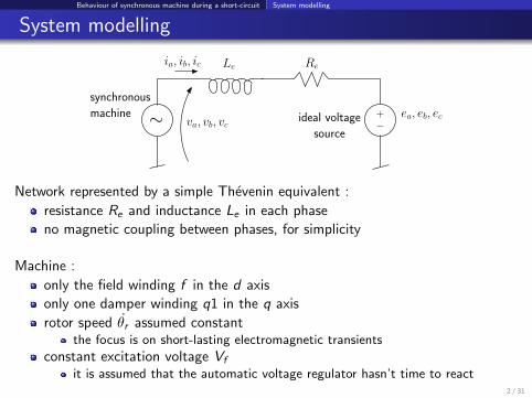
Network represented by a simple Thevenin equivalent :
resistance Re and inductance Le in each phase
no magnetic coupling between phases, for simplicity
Machine :
only the field winding f in the d axis
only one damper winding q1 in the q axis
rotor speed θr assumed constantthe focus is on short-lasting electromagnetic transients
constant excitation voltage Vf
it is assumed that the automatic voltage regulator hasn’t time to react2 / 31
Behaviour of synchronous machine during a short-circuit System modelling
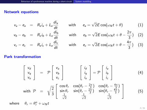
Network equations
va − ea = Re ia + Lediadt
with ea =√
2E cos(ωNt + θ) (1)
vb − eb = Re ib + Ledibdt
with eb =√
2E cos(ωNt + θ − 2π
3) (2)
vc − ec = Re ic + Ledicdt
with ec =√
2E cos(ωNt + θ − 4π
3) (3)
Park transformation
vd
vq
vo
= P
va
vb
vc
idiqio
= P
iaibic
(4)
with P =
√2
3
cos θr cos(θr − 2π3 ) cos(θr − 4π
3 )sin θr sin(θr − 2π
3 ) sin(θr − 4π3 )
1√2
1√2
1√2
(5)
where θr = θor + ωNt
3 / 31
Behaviour of synchronous machine during a short-circuit System modelling
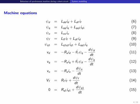
Machine equations
ψd = Ldd id + Ldf if (6)
ψq = Lqq iq + Lqq1iq1 (7)
ψo = Loo io (8)
ψf = Lff if + Ldf id (9)
ψq1 = Lq1q1iq1 + Lqq1iq (10)
vd = −Raid − θrψq −dψd
dt(11)
vq = −Raiq + θrψd −dψq
dt(12)
vo = −Raio −dψo
dt(13)
Vf = Rf if +dψf
dt(14)
0 = Rq1iq1 +dψq1
dt(15)
4 / 31

Behaviour of synchronous machine during a short-circuit System modelling
Variable - equations balance
19 variables : va, vb, vc , ia, ib, ic , vd , vq, vo , id , iq, io , ψd , ψq, ψo , ψf , ψq1, if , iq1
19 equations : (1 - 3), 6 eqs. in (4), (6 - 15)
Remarks
The model is made up of Differential-Algebraic Equations (DAEs)
some of the variables and some of the equations could be eliminated but theadditional computational effort of keeping all of them is negligible1
θr being known, the equations are linear with respect to the unknowns
some coefficients in these equations vary with time.
1not to mention the risk of introducing mistakes in analytical manipulations !5 / 31
Behaviour of synchronous machine during a short-circuit System modelling
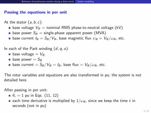
Passing the equations in per unit
At the stator (a, b, c):
base voltage VB = nominal RMS phase-to-neutral voltage (kV)
base power SB = single-phase apparent power (MVA)
base current IB = SB/VB , base magnetic flux ψB = VB/ωN , etc.
In each of the Park winding (d , q, o):
base voltage = VB
base power = SB
base current = SB/VB = IB , base flux = VB/ωN , etc.
The rotor variables and equations are also transformed in pu; the system is notdetailed here.
After passing in per unit:
θr = 1 pu in Eqs. (11, 12)
each time derivative is multiplied by 1/ωN , since we keep the time t inseconds (not in pu)
6 / 31
Behaviour of synchronous machine during a short-circuit System modelling
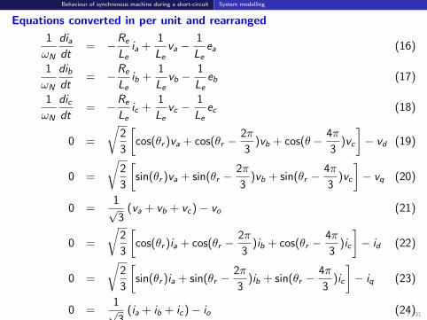
Equations converted in per unit and rearranged
1
ωN
diadt
= −Re
Leia +
1
Leva −
1
Leea (16)
1
ωN
dibdt
= −Re
Leib +
1
Levb −
1
Leeb (17)
1
ωN
dicdt
= −Re
Leic +
1
Levc −
1
Leec (18)
0 =
√2
3
[cos(θr )va + cos(θr −
2π
3)vb + cos(θ − 4π
3)vc
]− vd (19)
0 =
√2
3
[sin(θr )va + sin(θr −
2π
3)vb + sin(θr −
4π
3)vc
]− vq (20)
0 =1√3
(va + vb + vc )− vo (21)
0 =
√2
3
[cos(θr )ia + cos(θr −
2π
3)ib + cos(θr −
4π
3)ic
]− id (22)
0 =
√2
3
[sin(θr )ia + sin(θr −
2π
3)ib + sin(θr −
4π
3)ic
]− iq (23)
0 =1√3
(ia + ib + ic )− io (24)7 / 31

Behaviour of synchronous machine during a short-circuit System modelling
0 = Ldd id + Ldf if − ψd (25)
0 = Lqq iq + Lqq1iq1 − ψq (26)
0 = Lff if + Ldf id − ψf (27)
0 = Lq1q1iq1 + Lqq1iq − ψq1 (28)
0 = Loo io − ψo (29)
1
ωN
dψd
dt= −Raid − ψq − vd (30)
1
ωN
dψq
dt= −Raiq + ψd − vq (31)
1
ωN
dψf
dt= −Rf if + Vf (32)
1
ωN
dψq1
dt= −Rq1iq1 (33)
1
ωN
dψo
dt= −Raio − vo (34)
8 / 31
Behaviour of synchronous machine during a short-circuit System modelling
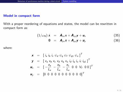
Model in compact form
With a proper reordering of equations and states, the model can be rewritten incompact form as:
(1/ωN ) x = Axxx + Axyy + ux (35)
0 = Ayxx + Ayyy + uy (36)
where:
x = [ ia ib ic ψd ψq ψf ψq1 ψo ]T
y = [ va vb vc vd vq vo id iq io if iq1 ]T
ux = [ − ea
Le− eb
Le− ec
Le0 0 Vf 0 0 ]T
uy = [0 0 0 0 0 0 0 0 0 0 0]T
9 / 31

Behaviour of synchronous machine during a short-circuit Numerical solution of the DAEs
Numerical solution of the DAEs
Let k denote the discrete time (k = 0, 1, 2, . . .), and h the time step size.
A popular numerical integration formula is the Trapezoidal Method :
xk+1 = xk +h
2(xk+1 + xk )
Replacing xk+1 by its expression (35) :
xk+1 = xk +h
2ωNAxxxk+1 +
h
2ωNAxyyk+1 +
h
2ωN ux k+1 +
h
2xk
Dividing byhωN
2and rearranging the various terms :[
Axx −2
hωNI
]xk+1 + Axyyk+1 = − 2
hωNxk −
1
ωNxk − ux k+1 (37)
where I is the unit matrix of same dimension as x .
10 / 31
Behaviour of synchronous machine during a short-circuit Numerical solution of the DAEs
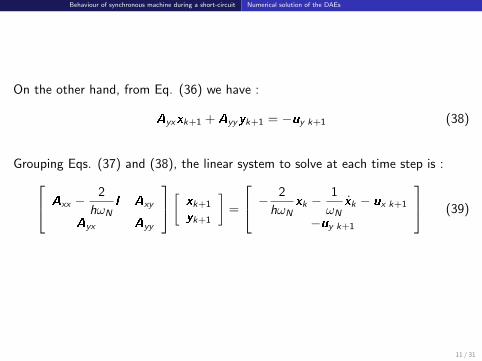
On the other hand, from Eq. (36) we have :
Ayxxk+1 + Ayyyk+1 = −uy k+1 (38)
Grouping Eqs. (37) and (38), the linear system to solve at each time step is : Axx −2
hωNI Axy
Ayx Ayy
[ xk+1
yk+1
]=
− 2
hωNxk −
1
ωNxk − ux k+1
−uy k+1
(39)
11 / 31
Behaviour of synchronous machine during a short-circuit Numerical example and comments on the results
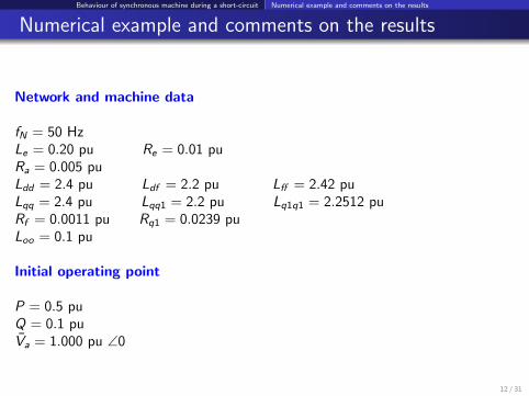
Numerical example and comments on the results
Network and machine data
fN = 50 HzLe = 0.20 pu Re = 0.01 puRa = 0.005 puLdd = 2.4 pu Ldf = 2.2 pu Lff = 2.42 puLqq = 2.4 pu Lqq1 = 2.2 pu Lq1q1 = 2.2512 puRf = 0.0011 pu Rq1 = 0.0239 puLoo = 0.1 pu
Initial operating point
P = 0.5 puQ = 0.1 puVa = 1.000 pu ∠0
12 / 31

Behaviour of synchronous machine during a short-circuit Numerical example and comments on the results
Simulation results
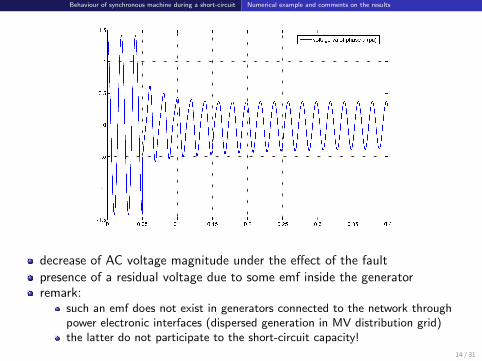
A three-phase short-circuit is simulated by setting E to zero at t = 0.05 s.
Important remark
The fault is not cleared in order to show the various time constants present in thecurrent evolution.
However, in practice:
the fault must be cleared fast enough, e.g. after 5 - 10 cycles (0.1 - 0.2 s)
beyond that time, the model is no longer valid:
rotor speed would not remain constantvf would be adjusted by the Automatic Voltage Regulatoretc.
13 / 31
Behaviour of synchronous machine during a short-circuit Numerical example and comments on the results
decrease of AC voltage magnitude under the effect of the fault
presence of a residual voltage due to some emf inside the generatorremark:
such an emf does not exist in generators connected to the network throughpower electronic interfaces (dispersed generation in MV distribution grid)the latter do not participate to the short-circuit capacity!
14 / 31
Behaviour of synchronous machine during a short-circuit Numerical example and comments on the results
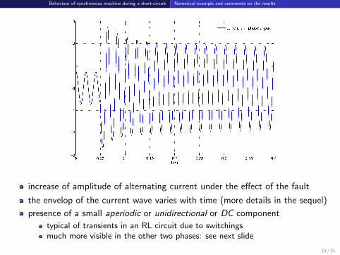
increase of amplitude of alternating current under the effect of the fault
the envelop of the current wave varies with time (more details in the sequel)
presence of a small aperiodic or unidirectional or DC component
typical of transients in an RL circuit due to switchingsmuch more visible in the other two phases: see next slide
15 / 31

Behaviour of synchronous machine during a short-circuit Numerical example and comments on the results
the magnitude of the aperiodic components decrease with a time constant' 0.15 s (in this example)the aperiodic components are not the same in all three phases, because therotor is not in the same position with respect to each stator windingonce they have vanished, the three phase currents become again sinusoidaland balanced
16 / 31

Behaviour of synchronous machine during a short-circuit Numerical example and comments on the results
the magnitude of the alternating component of ia shows two time constants:a short one, lasting a few cycles, resulting in a slightly higher initial amplitudeof the current: caused by damper winding q1a much longer one (' 1.5 s in this example): caused by field winding f
the current that the breakers have to interrupt is much higher than the onewhich would prevail in steady-state !the machine behaves initially as if it had a smaller internal reactance
17 / 31
Behaviour of synchronous machine during a short-circuit Numerical example and comments on the results
Magnetic fields
The alternating components of the stator currents ia, ib and ic
are shifted by ±2π/3 rad. They create a magnetic field HAC which rotates atthe angular speed ωN
this field is fixed with respect to the rotor windings
under the effect of the fault, the amplitude if ia, ib and ic increasessignificantly. So does the magnetic field HAC
this induces aperiodic current components in the rotor windings.
The aperiodic components of the stator currents ia, ib and ic
create a magnetic field HDC which is fixed with respect to the stator
hence it rotates at angular speed ωN with respect to the rotor windings
this induces alternating components of angular frequency ωN in the rotorwindings.
This is confirmed by the plots in the next slides.
18 / 31
Behaviour of synchronous machine during a short-circuit Numerical example and comments on the results
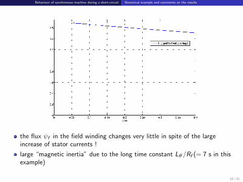
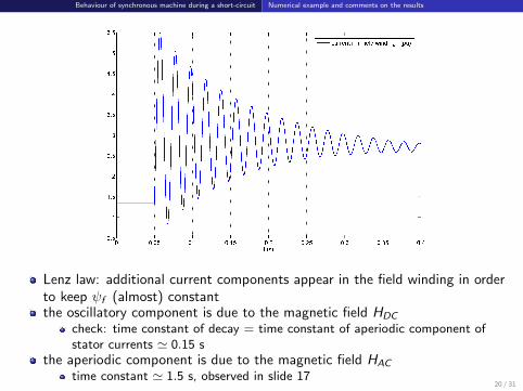
the flux ψf in the field winding changes very little in spite of the largeincrease of stator currents !
large “magnetic inertia” due to the long time constant Lff /Rf (= 7 s in thisexample)
19 / 31
Behaviour of synchronous machine during a short-circuit Numerical example and comments on the results
Lenz law: additional current components appear in the field winding in orderto keep ψf (almost) constantthe oscillatory component is due to the magnetic field HDC
check: time constant of decay = time constant of aperiodic component ofstator currents ' 0.15 s
the aperiodic component is due to the magnetic field HAC
time constant ' 1.5 s, observed in slide 1720 / 31
Behaviour of synchronous machine during a short-circuit Numerical example and comments on the results
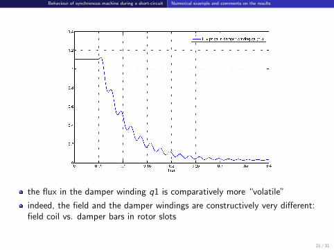
the flux in the damper winding q1 is comparatively more “volatile”
indeed, the field and the damper windings are constructively very different:field coil vs. damper bars in rotor slots
21 / 31
Behaviour of synchronous machine during a short-circuit Numerical example and comments on the results
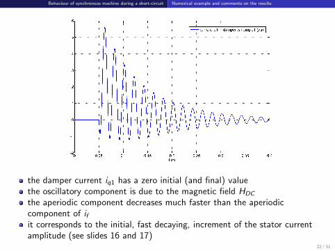
the damper current iq1 has a zero initial (and final) valuethe oscillatory component is due to the magnetic field HDC
the aperiodic component decreases much faster than the aperiodiccomponent of ifit corresponds to the initial, fast decaying, increment of the stator currentamplitude (see slides 16 and 17)
22 / 31
Behaviour of synchronous machine during a short-circuit Numerical example and comments on the results
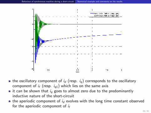
the oscillatory component of id (resp. iq) corresponds to the oscillatorycomponent of if (resp. iq1) which lies on the same axisit can be shown that iq goes to almost zero due to the predominantlyinductive nature of the short-circuitthe aperiodic component of id evolves with the long time constant observedfor the aperiodic component of if
23 / 31
Behaviour of synchronous machine during a short-circuit Numerical example and comments on the results
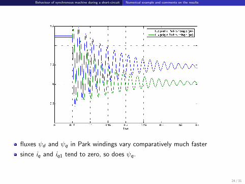
fluxes ψd and ψq in Park windings vary comparatively much faster
since iq and iq1 tend to zero, so does ψq.
24 / 31
Behaviour of synchronous machine during a short-circuit Numerical example and comments on the results
Simplified model of a synchronous machine for use inshort-circuit calculations
Usual simplifications for the computation of fault currents
The aperiodic components of the short-circuit currents are neglected
by the time the circuit breaker opens, these components are already smallthis approximation can be compensated by multiplying the fault current by anempirical factor larger than one
only the alternating components at frequency ωN are considered.
this allows using static computations as in sinusoidal steady-state !
Simple representation of the machine
in steady state, a (round-rotor) machine can be represented by the statorresistance and the synchronous reactance in series with an emf whosemagnitude is proportional to the field current
let us derive a similar model to represent the machine in the first cycles afterthe fault occurrence.
25 / 31
Behaviour of synchronous machine during a short-circuit Numerical example and comments on the results
Park equations of the machine:
vd = −Raid − θrψq −dψd
dt= −Raid − θr (Lqq iq + Lqq1 iq1)− dψd
dt(40)
vq = −Raiq + θrψd −dψq
dt= −Raiq + θr (Ldd id + Ldf if )− dψq
dt(41)
Just after the short-circuit, the fluxes ψf and ψq1 cannot change (much). On thecontrary, if and iq1 vary significantly to ensure constant fluxes.
Let us transform Eqs. (40, 41) to make ψf and ψq1 appear.
ψf = Lff if + Ldf id ⇒ if =ψf − Ldf id
Lff
ψq1 = Lq1q1iq1 + Lqq1iq1 ⇒ iq1 =ψq1 − Lqq1iq
Lq1q1
Introducing these expressions in Eqs. (40, 41):
vd = −Raid − θr (Lqq −L2qq1
Lq1q1)iq − θr
Lqq1
Lq1q1ψq1 −
dψd
dt(42)
vq = −Raiq + θr (Ldd −L2df
Lff)id + θr
Ldf
Lffψf −
dψq
dt(43)
26 / 31
Behaviour of synchronous machine during a short-circuit Numerical example and comments on the results
Simplifying assumptions
rotor speed : θr = ωN
the transformer emf’s are neglected :dψd
dt= 0
dψq
dt= 0
This leads to neglecting aperiodic components of short-circuit currents.
Eqs. (42, 43) become:
vd = −Raid − ωN (Lqq −L2qq1
Lq1q1)︸ ︷︷ ︸
L′′q
iq −ωNLqq1
Lq1q1ψq1︸ ︷︷ ︸
e′′d
= −Raid − X ′′q iq + e′′d (44)
vq = −Raiq + ωN (Ldd −L2df
Lff)︸ ︷︷ ︸
L′d
id +ωNLdf
Lffψf︸ ︷︷ ︸
e′q
= −Raiq + X ′d id + e′q (45)
Compare to the model in steady state:
vd = −Raid − ωNLqq iq = −Raid − Xq iq (46)
vq = −Raiq + ωNLdd id + Eq = −Raiq + Xd id + Eq (47)
27 / 31

Behaviour of synchronous machine during a short-circuit Numerical example and comments on the results
The models (44, 45) and (46, 47) are similar except for the following:
the direct-axis synchronous reactance Xd = ωNLdd is replaced by the smallerreactance X ′d = ωNL
′d
the quadrature-axis synchronous reactance Xq = ωNLqq is replaced by thesmaller reactance X ′′q = ωNL
′′q
the emf Eq, located along the q axis, is replaced by an emf with componentsin both axes
for some time after the fault inception, these components keep their pre-faultvalues (since they are proportional to fluxes).
Terminology
L′d (resp. X ′d ) is called the direct-axis transient inductance (resp. reactance)
it stems from the reaction of the field winding, whose dynamics are in theorder of a second
L′′q (resp. X ′′q ) is called the quadrature-axis subtransient inductance (resp.reactance)
it stems from the reaction of the damper winding, whose dynamics are in theorder of a few cycles
28 / 31
Behaviour of synchronous machine during a short-circuit Numerical example and comments on the results
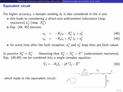
Equivalent circuit
For higher accuracy, a damper winding d1 is also considered in the d axis
this leads to considering a direct-axis subtransient inductance (resp.reactance) L′′d (resp. X ′′d )
Eqs. (44, 45) become:
vd = −Raid − X ′′q iq + e′′d (48)
vq = −Raiq + X ′′d id + e′′q (49)
for some time after the fault inception, e′′d and e′′q keep their pre-fault values
In practice X ′′d ' X ′′q . Assuming that X ′′d = X ′′q = X ′′ (subtransient reactance),Eqs. (48,49) can be combined into a single complex equation:
Va = −Ra Ia − jX ′′ Ia + E ′′ (50)
which leads to the equivalent circuit:
29 / 31

Behaviour of synchronous machine during a short-circuit Numerical example and comments on the results
Typical values
machine withround rotor salient poles
(pu) (pu)
Xd 1.5 - 2.5 0.9 - 1.5
X′
d 0.2 - 0.4 0.3 - 0.5
X′′
d 0.15 - 0.30 0.25 - 0.35
Xq 1.5 - 2.5 0.5 - 1.1
X′′
q 0.15 - 0.30 0.25 - 0.35
values in per unit on the machine base power and voltage
Remark
By considering that the rotor fluxes do not change, the computed current isthe one immediately after the faultthe curve in slide 17 shows that the current magnitude has somewhatdecreased by the time the breakers have to actwe are thus “on the safe side” (little higher current).
30 / 31
Behaviour of synchronous machine during a short-circuit Numerical example and comments on the results
How determine the emf E ′′ ?
Let tsc be the instant of the short-circuit inception.
E ′′ being the same just after and before the fault:
E ′′(t+sc ) = E ′′(t−sc )
while using Eq. (50):
E ′′(t−sc ) = Va(t−sc ) + Ra Ia(t−sc ) + jX ′′ Ia(t−sc )
Va(t−sc ) and Ia(t−sc ) are provided by a power flow computation performed in thepre-fault configuration.
P(t−sc ) + jQ(t−sc ) = Va(t−sc ) I ?a (t−sc ) ⇒ Ia(t−sc ) =P(t−sc )− jQ(t−sc )
V ?a (t−sc )
31 / 31