elec0029 - electric power systems analysis the...

ELEC0029 - Electric power systems analysis

The power flow computation

Thierry Van [email protected] www.montefiore.ulg.ac.be/~vct

February 2020

1 / 32

The power flow computation

English terminology:

load flow computation

power flow computation (preferred)

Termes francais :

calcul de repartition de charge

calcul d’ecoulement de charge

calcul d’ecoulement de puissance.

Objective: determine the electrical state of a network (voltages at all buses,currents in all branches, losses, etc.) from consumptions and productions specifiedat its various buses.

Certainly the most used computation in electric power systems !

2 / 32

The power flow computation Power flow equations

Power flow equations

“Multi-purpose” two-port

To model:

a line or a cable: set nij = 1 and φij = 0

a standard transformer: set Bsji = 0 and φij = 0

a phase-shifting transformer: set Bsji = 0 and φij 6= 0

Iij = jBsij Vi + Yij(Vi −Vj

nije−jφij ) = jBsij Vi + (Gij + jBij)(Vi −

Vj

nije−jφij )

3 / 32


Power balances at the network buses

Ii = j Bsi Vi +∑

j∈N (i)

Iij i = 1, . . . ,N

⇔ Pi + jQi = Vi I?i = −jBsiV

2i +

∑j∈N (i)

Vi I?ij i = 1, . . . ,N

4 / 32


Pi + jQi = −jBsiV2i +

∑j∈N (i)

Vi I?ij

= −jBsiV2i − j

∑j∈N (i)

BsijV2i +

∑j∈N (i)

Vi (Gij − jBij)(V ?i −

V ?j

nije jφij )

= −jBsiV2i − j

∑j∈N (i)

BsijV2i +

∑j∈N (i)

(Gij − jBij)(V 2i −

ViVj

nije j(θi−θj+φij ))

Pi =∑

j∈N (i)

GijV2i −

∑j∈N (i)

ViVj

nij[Gij cos(θi − θj + φij) + Bij sin(θi − θj + φij)]

︸︷︷︸fi (. . . ,Vi , θi , . . .)

Qi = −(Bsi +∑

j∈N (i)

Bsij +∑

j∈N (i)

Bij)V2i +

+∑

j∈N (i)

ViVj

nij[Bij cos(θi − θj + φij)− Gij sin(θi − θj + φij)]

︸︷︷︸gi (. . . ,Vi , θi , . . .)

5 / 32

The power flow computation Data specification

Data specification

PV BUSPQ BUSPQ BUS BUS

LOAD & GENERATOR BUS

PQ BUS PV BUS

SLACK BUSLOAD BUS GENERATOR BUS

U N K N O W N S

E Q U A T I O N S

by substituting voltage magnitudes and phase angles in the non used power balance equation, one obtains:

QgNP g

N

VN = V oN

θN = 0

QgN

P gN

VN 6 θN

QgiQg

i

Qgi

P gi

Vi 6 θi

P ci

Qci

Vi 6 θi

Qgi

P gi

Qci

P ci

Vi 6 θi

θiθiθiθiθiVi Vi Vi

Vi = V oiVi = V o

i

P gi = fi(. . .)

Qgi = gi(. . .)−Qc

i = gi(. . .)

P gi − P c

i = fi(. . .)

Qgi −Qc

i = gi(. . .)

−P ci = fi(. . .)

Vθ

6 / 32

The power flow computation The role of the slack bus

The role of the slack bus

1.One cannot specify the active powers injected Pi at all buses since:

N∑i=1

Pi = active losses = p (. . . ,Vi , θi , . . .)︸︷︷︸??

2.

the voltage phase angles θi appear in the eqs. through differences only

one may add an arbitrary constant c to all phase angles without changing theelectric state of the network

one bus must be taken as phase angle reference.

Slack bus: let us assume it is the N-th bus:

active power balance equation replaced by:

θN = 0 (0 : arbitrary value)

7 / 32

The power flow computation The role of the slack bus

Which bus take as slack bus?

At this bus, the active power injection will take the value:

PN = −N−1∑i=1

Pi + p

where all Pi ’s in the sum are data and p is known at the end of the computation

⇒ select a bus to which a generator is connected (= slack generator)

What about reactive losses and the role of the slack bus?

one cannot specify the reactive power injections at all buses

luckily, they are not imposed at the PV buses !

⇒ no problem as long as there are one or more PV buses in the data(for reactive power, each PV bus acts as a slack bus).

Which data specify at the slack bus?

either the voltage V or the reactive power injection Q

since a generator is connected, it is natural to specify the voltage V .8 / 32

The power flow computation Power flow equations in vector form

Power flow equations in vector form

NPV : nb of PV buses NPQ : nb of PQ buses NPV + NPQ + 1 = N

v vector of voltage magnitudes at all buses (dim. N)θ vector of voltage phase angles at all buses (dim. N)po vector of specified active power injections at PV or PQ buses (dim. N − 1)qo vector of specified reactive power injections at PQ buses (dim. NPQ)v o vector of specified voltage magnitudes at PV and slack buses (dim NPV + 1)

N − 1 active power balance equations at PV and PQ buses:

f (v ,θ)− po = 0

1 phase angle equation at the slack bus:

θN = 0

NPQ reactive power balance equations at PQ buses:

g(v ,θ)− qo = 0

NPV + 1 voltage equations at the PV and slack buses:

v − v o = 09 / 32

The power flow computation Solving the equations numerically

Solving the equations numerically

Newton(-Raphson) method: case of a scalar function of a single variable

Let the equation be: ϕ(x) = 0. We note ϕx =dϕ

dx.

Starting from an initial value (“guess”) x (0), the following sequence is computed:

x (k+1) = x (k) − ϕ(x (k))

ϕx(x (k))k = 0, 1, 2, . . .

until: |ϕ(x (k+1))| < ε

For x (0) “sufficiently close” to the solution, the convergence is fast (quadratic).10 / 32


Newton method: case of a vector function of several variables

Let the equation be: ϕ(x) = 0

The Jacobian (matrix) of ϕ with respect to x is defined by:

[ϕx ]ij =∂ϕi

∂xj

Starting from an initial value (“guess”) x (0), the following sequence is computed:

x (k+1) = x (k) − [ϕx(x (k))]−1ϕ(x (k)) k = 0, 1, 2, . . .

until: maxi |ϕi (x(k+1))| < ε.

In pratice, the Jacobian is not inverted. Instead, the linear system:

ϕx(x (k)) ∆x = −ϕ(x (k))

is solved and x is incremented according to:

x (k+1) = x (k) + ∆x

11 / 32


Solving the linear system

Factorization (or LDU decomposition) of the Jacobian:

ϕx = LDU

Substitution of the right-hand side term:

ϕx∆x = −ϕ ⇔ LDU∆x = −ϕ

one solves successively:

Ly = −ϕU∆x = D−1y

which is easy owing to the triangular structure of the matrices.12 / 32


Application to power flow equations

Structure of Jacobian:

ϕx =

fv fθ0 eNgv gθU 0

eN : unit row vector of dimension NU : matrix whose entries are 0’s and 1’sEach of the four sub-matrices of dimension N × N.

The matrix ϕx is sparse: most of the elements are zero, since a power injection atone bus involves only the voltages at this bus and at its direct neighbours.

only the nonzero terms are stored, in a compact way (accessed throughpointers)

useless operations involving zero’s are avoided (sparsity programming)

the number of nonzero terms created during the factorization (fill-in terms) iskept as low as possible, by permuting rows and columns: optimal ordering

the pattern of nonzero terms is analyzed, often before the factorization step.

13 / 32


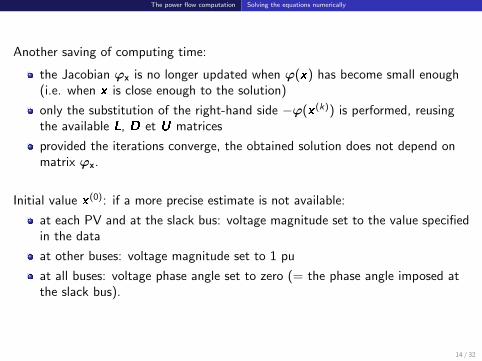
Another saving of computing time:

the Jacobian ϕx is no longer updated when ϕ(x) has become small enough(i.e. when x is close enough to the solution)

only the substitution of the right-hand side −ϕ(x (k)) is performed, reusingthe available L, D et U matrices

provided the iterations converge, the obtained solution does not depend onmatrix ϕx.

Initial value x (0): if a more precise estimate is not available:

at each PV and at the slack bus: voltage magnitude set to the value specifiedin the data

at other buses: voltage magnitude set to 1 pu

at all buses: voltage phase angle set to zero (= the phase angle imposed atthe slack bus).

14 / 32

The power flow computation Taking operating constraints into account

Taking operating constraints into account

If the solution does not obey an operating constraint:

h(v ,θ) ≤ 0

one can enforce:h(v ,θ) = 0

provided that another equation is removed.

The resulting new set of equations is solved. The procedure is repeated if needed.

Important case : reactive power limits of generators at PV buses

Qmini ≤ Qi (v ,θ) ≤ Qmax

i

if Qi (v ,θ) > Qmaxi : the bus is switched from PV to PQ type, with Qi = Qmax

i

Vi becomes variable: Vi = V oi → Vi ≤ V o

i

if Qi (v ,θ) < Qmini : the bus is switched from PV to PQ type, with Qi = Qmin

i

Vi becomes variable: Vi = V oi → Vi ≥ V o

i .15 / 32

The power flow computation Taking operating constraints into account

Newton method with enforcement of generator reactive power limits

1 k := 0 ; v (0) = v o ; θ(0) = θo

2 compute f (v (k),θ(k))− po and g(v (k),θ(k))− qo

3 if maxi |gi (v (k),θ(k))− Qoi | < δQ :

check generator reactive power limits ;if some limits exceeded :

switch the corresponding buses from PV to PQgo to 2 ;

4 if maxi |fi (v (k),θ(k))− Poi | < εP and maxi |gi (v (k),θ(k))− Qo

i | < εQ :stop ;

5 if k = 0 or maxi |fi (v (k),θ(k))−Poi | > βP or maxi |gi (v (k),θ(k))−Qo

i | > βQ :

compute and factorize the Jacobian: ϕx = LDU

6 (substitution:) solve LDU

[∆v

∆θ

]=

[po − f (v (k),θ(k))qo − g(v (k),θ(k))

]7 v (k+1) = v (k) + ∆v ; θ(k+1) = θ(k) + ∆θ

8 k := k + 1 ; go to 2.

16 / 32

The power flow computation Iterative processing of losses

Iterative processing of losses

1 Estimate the network (active power) losses. Let us denote them by p.2 Share the sum of all loads and losses among the various generators, including

the slack generator.

Estimated slack generator production: PN = −N−1∑i=1

Pi + p.

3 Run the power flow computation. This provides updated values of the lossesp and the slack generator production PN . Both are linked by:

PN = −N−1∑i=1

Pi + p

and hence:PN − PN = p − p

4 If |PN − PN | is too large:adjust again the productions, using p as the new estimate of the lossesgo to 3.

Else, stop.

In practice, no more than one iteration needed (i.e. 2 power flow computations).17 / 32

The power flow computation Distributed slack buses

Distributed slack buses

Share active power balancing among several generators (not just one)

−→ distributed slack buses

Let us define an additional variable ∆Pg used to adjust the generations:

at the i-th bus (i = 1, . . . ,N) a fraction αi of ∆Pg is assigned:

Pi = Poi + αi∆Pg with

N∑i=1

αi = 1

if the i-th bus has no generator or has a generator not taking part inbalancing:

αi = 0

The vector of bus active power injections can be written as:

p = po + ∆Pg α with α = [α1, α2, . . . , αN ]T

18 / 32

The power flow computation Distributed slack buses

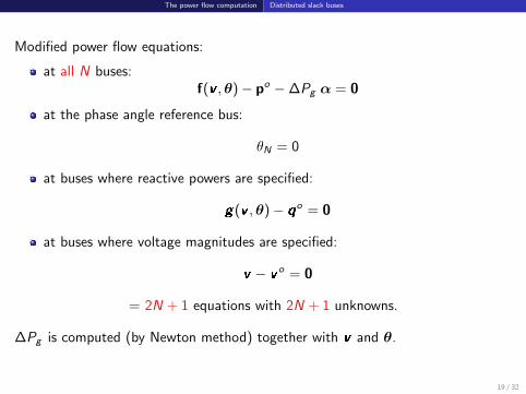
Modified power flow equations:

at all N buses:f(v ,θ)− po −∆Pg α = 0

at the phase angle reference bus:

θN = 0

at buses where reactive powers are specified:

g(v ,θ)− qo = 0

at buses where voltage magnitudes are specified:

v − v o = 0

= 2N + 1 equations with 2N + 1 unknowns.

∆Pg is computed (by Newton method) together with v and θ.

19 / 32

The power flow computation Adjusting the transformer ratios

Adjusting the transformer ratios

Why?

To keep the voltages V at some buses at specified values V o

to reflect an operating practice (operator adjusting transformers from acontrol center) or an automatic control device (load tap changer).

How?

Ratios treated as continuous variables (approximation) or as discrete ones(corresponding to the tap positions)

variation in constant steps or proportional to the deviation of voltage withrespect to its set-point (|V − V o |)taking in account the range of variation of each ratio (min/max tap positions)

after the ratios have been adjusted, a new sequence of Newton iterations isperformed

the procedure is repeated until no ratio changes any further.

20 / 32

The power flow computation Electrical decoupling

Electrical decoupling

Pi =∑

j∈N (i)

GijV2i −

∑j∈N (i)

ViVj


∂Pi

∂Vi= 2Vi

∑j∈N (i)

Gij −∑

j∈N (i)

Vj


∂Pi

∂Vj= −Vi


∂Pi

∂θi=

∑j∈N (i)

ViVj

nij[Gij sin(θi − θj + φij)− Bij cos(θi − θj + φij)]

∂Pi

∂θj= −ViVj

nij[Gij sin(θi − θj + φij)− Bij cos(θi − θj + φij)]

Assuming that Vi = Vj = nij ' 1 pu and θi − θj + φij ' 0 :

∂Pi

∂Vi'∑

j∈N (i)

Gij∂Pi

∂Vj' −Gij

∂Pi

∂θi' −

∑j∈N (i)

Bij∂Pi

∂θj' Bij

Gij � |Bij | ⇒ |∂Pi

∂Vi|, |∂Pi

∂Vj| � |∂Pi

∂θi|, |∂Pi

∂θj|

21 / 32


Qi = −[Bsi+∑

j∈N (i)

(Bsij+Bij)]V 2i +

∑j∈N (i)

ViVj


∂Qi

∂Vi= −2[Bsi +

∑j

(Bsij + Bij)]Vi +∑j

Vj


∂Qi

∂Vj=

Vi


∂Qi

∂θi= −

∑j∈N (i)

ViVj

nij[Bij sin(θi − θj + φij) + Gij cos(θi − θj + φij)]

∂Qi

∂θj=

ViVj

nij[Bij sin(θi − θj + φij) + Gij cos(θi − θj + φij)]

Assuming that Vi = Vj = nij ' 1 pu and θi − θj + φij ' 0 :

∂Qi

∂Vi' −2[Bsi +

∑j

Bsij ]−∑j

Bij∂Qi

∂Vj' Bij

∂Qi

∂θi= −

∑j

Gij∂Qi

∂θj' Gij

Gij � |Bij | ⇒ |∂Qi

∂Vi|, |∂Qi

∂Vj| � |∂Qi

∂θi|, |∂Qi

∂θj|

22 / 32


Jacobian matrix:

full: ϕx =

fv fθ0 eNgv gθU 0

approximate: ϕx '

0 fθ0 eNgv 0U 0

fθ dominant compared to fv gv dominant compared to gθ.

Fast decoupled Newton method:

system of 2N equations decomposed into two systems of N equations

each Newton iteration decomposed into : one half-iteration to update thephase angles, followed by one half-iteration to update the voltage magnitudes

active power and phase reference (θN = 0) equations solved using the

sub-matrix

[fθeN

]to update the voltage phase angles

reactive power and voltage equations solved using the sub-matrix

[gv

U

]to update the voltage magnitudes.

23 / 32

The power flow computation The “DC” power flow approximation

The “DC” power flow approximation

Simplified power flow equations obtained after:

linearizing the variation of active power with voltage phase angles

neglecting the active power losses in all branches

assuming all voltage magnitudes equal to 1 pu

neglecting all reactive power flows in branches.

Linear model used:

to simplify some computations, e.g.

to perform a very large number of power flow computations: a single linearsystem of half size is solvedwhen the power flow equations are included as constraints in a largeoptimization problem (Optimal power flow)

to easily cumulate the effects of several modifications applied to the system(thanks to linearity).

24 / 32


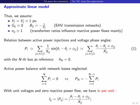
Approximate linear model

Thus, we assume:Vi = Vj ' 1 puGij ' 0 Bij = − 1

Xij(EHV transmission networks)

nij ' 1 (transformer ratios influence reactive power flows mainly)

Relation between active power injections and voltage phase angles:

Pi '∑

j∈N (i)

1

Xijsin(θi − θj + φij) '

∑j∈N (i)

θi − θj + φijXij

(1)

with the N-th bus as reference: θN = 0.

Active power balance with network losses neglected:

N∑i=1

Pi = 0 ⇔ PN = −N−1∑i=1

Pi

With unit voltages and zero reactive power flow, we have in per unit :

Iij = |Pij | = |θi − θj + φijXij

|25 / 32


Matrix form

Let us assume for simplicity that there is no phase shifting transformer:

φij = 0

By grouping the equations (1) relative to buses 1 to N − 1 :

po = A θ

where A is defined by:

[A]ij = − 1

Xiji , j = 1, . . . ,N − 1; i 6= j

[A]ii =∑

j∈N (i)

1

Xiji = 1, . . . ,N − 1

26 / 32


Example

Phase angle reference at bus 4: θ4 = 0 P1

− P2

− P3

=

1

X12+ 1

X13+ 1

X14− 1

X12− 1

X13

− 1X12

1X12

+ 1X24

0

− 1X13

0 1X13

+ 1X34

θ1

θ2

θ3

Active power balance: P1 − P2 − P3 + P4 = 0

27 / 32


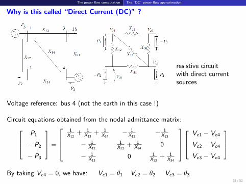
Why is this called “Direct Current (DC)” ?

resistive circuitwith direct currentsources

Voltage reference: bus 4 (not the earth in this case !)

Circuit equations obtained from the nodal admittance matrix: P1

− P2

− P3

=

1

X12+ 1

X13+ 1

X14− 1

X12− 1

X13

− 1X12

1X12

+ 1X24

0

− 1X13

0 1X13

+ 1X34

Vc1 − Vc4

Vc2 − Vc4

Vc3 − Vc4

By taking Vc4 = 0, we have: Vc1 = θ1 Vc2 = θ2 Vc3 = θ3

28 / 32


Sensitivity analysis

Power flow equations in compact vector form:

ϕ(x ,p) = 0 (2)

x : vector of voltage magnitudes and phase angles (dim. n) (state vector)p : vector of parameters (dim. m)

Let x? be the solution of (2) corresponding to p = p?

η(x ,p) be a variable of interest.

How does η vary when the parameters p are varied from p? to p? + ∆p ?

“Brute-force” solution

Solve (2) for p = p? + ∆p, i.e. compute ∆x such that:

ϕ(x? + ∆x ,p? + ∆p) = 0

and compute the corresponding new value: η(x? + ∆x ,p? + ∆p).

29 / 32


Elegant solution

Compute directly the sensitivities: Sηp =

lim

∆p1→0

∆η

∆p1...

lim∆pm→0

∆η

∆pm

For infinitesimal variations denoted by d . :

ϕ(x? + dx ,p? + dp) ' ϕ(x?,p?) +ϕx dx +ϕp dp = ϕx dx +ϕp dp = 0

and hence, assuming that ϕx is non-singular:

dx = −ϕ−1xϕp dp (3)

By linearizing η :

dη =∑i

∂η

∂pidpi +

∑i

∂η

∂xidxi = dpT∇pη + dxT∇xη

where ∇pη =

∂η∂p1

...∂η∂pm

∇xη =

∂η∂x1

...∂η∂xn

30 / 32


Replacing dx by its expression (3):

dη = dpT∇pη − dpTϕTp

(ϕTx

)−1∇xη = dpT[∇pη −ϕT

p

(ϕTx

)−1∇xη]

which gives the sought sensitivities: Sηp = ∇pη −ϕTp

(ϕTx

)−1∇xη

Practical procedure

1 compute ∇xη , ∇pη and ϕp2 ϕx being available in factorized form (LDU), solve: ϕT

x y = ∇xη3 compute Sηp = ∇pη −ϕT

p y.

Examples

Sensitivities to the bus active and reactive powers:

p =

[po

qo

]and ϕp = −

Up

0Uq

0

Up, Uq : matrices including 0’s and 1’s.

31 / 32


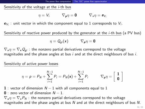
Sensitivity of the voltage at the i-th bus

η = Vi ∇pη = 0 ∇xη = eVi

eVi : unit vector in which the component equal to 1 corresponds to Vi .

Sensitivity of reactive power produced by the generator at the i-th bus (a PV bus)

η = Qgi (x) ∇pη = 0

∇xη = ∇xQgi : the nonzero partial derivatives correspond to the voltagemagnitudes and the phase angles at bus i and at the direct neighbours of bus i .

Sensitivity of active power losses

η = p = PN +N−1∑i=1

Pi = PN(x) +N−1∑i=1

Pi ∇pη =

[10

]1 : vector of dimension N − 1 with all components equal to 10 : zero vector of dimension N − 1.∇xη = ∇xPN : the nonzero partial derivatives correspond to the voltagemagnitudes and the phase angles at bus N and at the direct neighbours of bus N.

32 / 32

elec0029 - electric power systems analysis the...

Documents