behavioral price discrimination in a distribution...

1

Behavioral Price Discrimination in a Distribution Channel: A Dynamic Pricing Perspective

Koray Cosguner †

Assistant Professor of Marketing, Georgia State University

Tat Chan

Associate Professor of Marketing, Washington University in St. Louis

P.B. (Seethu) Seetharaman

W. Patrick McGinnis Professor of Marketing, Washington University in St. Louis

July 3, 2014

† Corresponding Author: Koray Cosguner, email: [email protected]; Ph: 404-413-7697. This article is based on the first author’s doctoral

dissertation, written at Olin Business School under the supervision of the second and third authors. The authors thank seminar participants at Olin, Georgia State, Yale, Rice, Alberta, Johns Hopkins, Emory, Carnegie Mellon, Koc, Sabanci, HEC, and Ozyegin for their comments and feedback on earlier versions of this article.

2

Behavioral Price Discrimination in a Distribution Channel: A Dynamic Pricing Perspective

Abstract

We study behavioral price discrimination in a distribution channel in the presence of demand

inertia. Unlike previous empirical studies of behavioral price discrimination, which rely only on estimated

differences in price elasticity across customers, our structural approach additionally relies on estimated

differences in price elasticity across time. In doing this, we explicitly account for dynamic pricing effects

– which represent how current price of a brand both responds to past demand, as well as influences future

demand, of all brands in the category – on channel members’ behavioral price discrimination incentives.

We model the pricing decisions of not only brand manufacturers (who set wholesale prices) but also the

retailer (who sets retail prices). We find that price discrimination over time is as important as price

discrimination across customer segments. We find that the retailer can outsource the data analytics and

price customization to manufacturers, by selling its customer database to them, and improve retail profit

by 29 % compared to the case of mass market pricing. Instead, taking charge of the price discrimination

on its own improves retail profit by only 12 %. Interestingly, we find that inducing manufacturers to

behaviorally price discriminate across different customers ends up making the manufacturers worse off

compared to the case of no price discrimination. This illustrates that information is a potent source of

channel power to the retailer in inertial markets. Last, but not least, we find that just exploiting the most

recent purchase of customers for price discrimination purposes yields 52% of the net profit gain that

accrues to the retailer by additionally exploiting segment membership information of customers.

Keywords: Behavioral Price Discrimination, Dynamic Pricing, Targeted Coupons, Inertia.

3

Introduction

When pricing strategies of firms recognize the future (i.e., long-term) implications – for

consumers and competitors – of their current prices, dynamic pricing is said to exist. Such dynamic

pricing incentives often arise in product markets which are characterized by switching costs that arise due

to inertia in consumers’ brand choices over time. Inertia refers to the phenomenon of consumers often

repeat-purchasing the same brand on successive purchase occasions. Such inertial, or habitual, brand

choice behavior of consumers, in turn, leads to the aggregate (e.g., market-level) demand for a brand

being positively correlated over time.

One pricing implication of inertia in demand is that manufacturers or retailers can target price-off

coupons to consumers that are based on these consumers’ most recently purchased brands. For example,

consumers who bought Coke most recently in the cola category may receive a price-off coupon in the

mail for Pepsi, while those who bought Pepsi most recently may receive a coupon for Coke. Such

behavioral price discriminationi (BPD henceforth) is enabled by the fact that customers’ most recent

purchases are observed in retail transactional data collected using retailers’ loyalty cards (such as the

Kroger Rewards card). From such customer-level transactional data, suppose that the brand manager of

Coke observes that John Doe’s most recently purchased brand in the cola category is Pepsi. Knowing that

John Doe’s conditional brand choice probability for Pepsi is now higher on account of his demand inertia,

the brand manager of Coke realizes that she must offer John Doe a price discount on Coke in order to

induce him to buy Coke next time instead of Pepsi. The brand manager of Pepsi faces a similar pressure

to lure previous buyers of Coke using price discounts. Such competitive pressures among Coke and Pepsi

to “poach” each other’s customers weaken each brand’s incentive to “milk” their installed customer base

(i.e., most recent buyers) by charging them higher prices (to exploit their inertia). In other words, even

though a monopoly firm has an incentive to behaviorally price discriminate, i.e., BPD, between its

existing (inertia-prone / less price elastic) and new (inertia-insensitive / more price elastic) customers by

charging them higher and lower prices, respectively, thus improving the monopoly firm’s profit, a

4

duopoly (or, more generally, oligopoly) firm may hurt from such BPD if the “poaching” pressure

overwhelms the “milking” incentive and decreases competing firms’ profits.

When the analysis of BPD in an oligopoly in the presence of inertia, as discussed above, is

applied to a packaged goods category (such as cola, with major brands Coke and Pepsi), the strategic role

of the retailer in setting retail prices and, therefore, targeted retail coupons, for the brands cannot be

ignored. For example, being a category profit maximizer, the retailer does not face the “poaching”

pressure that competing brand manufacturers are faced with. Therefore, the retailer has the ability to

potentially extract the full benefits of BPD. At the same time, since the retailer takes the wholesale prices

from the manufacturers as a given before making retail pricing decisions (i.e., sequentially moves after

the manufacturers in a Stackelberg pricing game), the manufacturers could anticipate the retailer’s

behavior and, therefore, appropriately modify their upstream wholesale prices. Manufacturers could also

drop targeted coupons that by-pass the retailer and directly incentivize end consumers to buy their brands.

Such efforts by manufacturers could limit the retailer’s ability to seek disproportionate rents from BPD in

the channel. Given these issues, it is necessary to carefully analyze the BPD implications of inertial

demand for all players – manufacturers and the retailer -- within the distribution channel. This has not

been done in previous research. Therefore, the primary objective of this research is to model BPD within

a distribution channel in a market with inertial demand.

We take an empirical approach to achieve our above-mentioned objective. We rely on structural

estimates of consumer demand and firm pricing behavior, obtained for a duopoly market using actual

market data on demand and prices, to perform counterfactual experiments regarding BPD. In doing this,

we generalize the existing, albeit limited, literature on structural models of targeted coupons within a

distribution channel to handle dynamic pricing effects. Unlike previous structural models of targeted

coupons, which rely only on estimated differences in price elasticity across customer segments, our

structural model additionally relies on estimated differences in price elasticity across time for each

customer (that arise on account of temporal differences in the identity of the customer’s most recently

bought brand in the category). This, in turn, implies that our structural approach yields targeted coupon

5

values both across customer segments (as in existing structural models), as well as across time for each

customer segment. This allows us to understand the profit impact, for each player in the distribution

channel, of exploiting an additional source of price elasticity variation (i.e., across time) in the market.

In order to deliver on our research objective, we do the following: We first estimate an inertial

demand model using household-level brand choice data in the cola category from a single store. The

estimation of the demand model explicitly accommodates differences across customer segments in terms

of their preference parameters. The estimated demand model then serves as an input to a dynamic

structural pricing model within the distribution channel, whose parameters are estimated using retail

tracking data on brands’ prices over time at the same store. Using the estimated parameters of the

structural demand and pricing models, we perform a counterfactual experiment in which we allow the

retailer to engage in BPD using targeted coupons that exploit differences among customers in terms of

both their estimated segment membership, as well as the identity of their previously purchased cola brand.

This counterfactual experiment allows us to quantify the pricing and profit impact to all channel

participants of the retailer’s BPD in the presence of inertia. We then perform a second counterfactual

experiment in which we allow the manufacturers (one at a time or both simultaneously) to directly engage

in BPD by directly dropping targeted manufacturer coupons to consumers, which also influences the retail

prices chosen by the retailer. Comparing the resulting prices and profits to those obtained in the first

counterfactual experiment allows us to understand whether a manufacturer could overcome the loss of

control that is associated with letting the retailer determine the targeted coupons by taking charge of the

BPD. Comparing the sub-cases (corresponding to only one manufacturer employing BPD versus both)

under this second counterfactual experiment allows us to understand whether there are Prisoner’s

dilemma considerations that arise in the manufacturers’ employment of BPD in the presence of inertial

demand. Within each of the two counterfactual experiments discussed above, we compare the

consequences of exploiting differences in price elasticity only across customers (as in previously

proposed structural models of targeted coupons), versus across both customers and time (as in our

proposed structural model of targeted coupons).

6

Our key findings are summarized here. First, the retailer and Pepsi both benefit (i.e., their profits

increase), while Coke hurts (i.e., its profit decreases) from the retailer engaging in BPD. Second, the

retailer can more than double their incremental profit from BPD by exploiting the most recent purchase

information of each customer in addition to their segment membership, when compared to exploiting

segment membership only. In other words, price discrimination over time is as important as, if not more

important than, price discrimination across customer segments. This is a new finding to the literature on

BPD and implies that a substantively significant increase in retail profit could accrue at little to no

analytical cost since tracking the most recent purchase outcome of a customer is very easy from a

database management standpoint for a retailer. Third, the retailer and Pepsi both benefit (i.e., their profits

increase), while Coke hurts (i.e., its profit decreases), when both manufacturers jointly engage in BPD, as

opposed to the retailer doing BPD. In other words, the retailer can simply outsource the data analytics

and customization of coupons to the two manufacturers and improve its profit beyond what it can achieve

by proactively engaging in analytics and customization on its own. Fourth, it is better for the retailer to

share its customer database on a non-exclusive basis with both manufacturers, than to share the data with

one manufacturer only or with neither. Fifth, if the retailer can charge the manufacturers for access to its

customer database, its profit improves by a further 17 % over the profit obtained by managing BPD on its

own (which itself is 12 % higher than the profit obtained using mass market pricing). In other words,

serving as an information broker to sell transactional data to product manufacturers can be a vital

source of business profit to the retailer. Sixth, while the retailer benefits from inducing manufacturers to

behaviorally price discriminate by dropping customized coupons to different customer types, it ends up

making the manufacturers worse off than under the case of no price discrimination! This illustrates that

information is a potent source of channel power to the retailer in the presence of inertial demand. Last,

but not least, we find that BPD based only on the customer’s most recent purchase yields 52 % of the net

profit gain that accrues to the retailer from BPD that simultaneously exploits the customer’s segment

membership and most recent purchase. Considering that tracking the most recent purchase of each

customer in the retailer’s data warehouse is a much easier task than calculating the segment membership

7

(using the customer’s full purchase history), it is remarkable that such a meaningful retail profit lift can

be obtained by using such a simple summary statistic about customer behavior.

The rest of the paper is organized as follows. In the next section, we review pertinent literature.

Section 3 presents our structural model of BPD within the distribution channel. Empirical results are

discussed in Section 4. Section 5 concludes.

Pertinent Literature

BPD Without Inertia – Analytical Results: Thisse and Vives (1988) find that while a monopolist

unequivocally benefits from price discrimination, competing firms may get trapped in to a prisoner’s

dilemma where all firms price discriminate but make lower profits. Shaffer and Zhang (1995) obtain the

same prisoner’s dilemma result when targeted coupons at brand switchers are used by competing firms as

vehicles of BPD. Villas-Boas (1999) and Fudenberg and Tirole (2000) both show that firms set lower

prices to attract competitors’ previous customers, with the former also finding that greater consumer

patience intensifies competition, while greater firm patience softens competition, among duopoly firms.

Chen, Narasimhan and Zhang (2001) qualify the main result in Shaffer and Zhang (1995) by showing that

the prisoner’s dilemma result goes away if consumer targeting is imprecise enough, in which case

competing firms increase their profits from using BPD. Acquisiti and Varian (2006) show that targeted

pricing is profitable only if a large enough fraction of consumers are myopic but if consumers are

forward-looking, the firm must offer higher service with higher prices to keep targeted pricing profitable.

Pazgal and Soberman (2008) show that targeted price/service competition can hurt competing firms by

making them compete fiercely to build up new customers and, therefore, a behavioral database to exploit

for targeted pricing. Liu and Zhang (2006) study targeted pricing by the retailer accounting for the

strategic role of the manufacturer within the distribution channel. They show that targeted pricing may not

be beneficial to the retailer because the manufacturer can take advantage of downstream targeted pricing

by raising its wholesale price at the expense of the retailer. Shin and Sudhir (2010) show that BPD can

improve competing firms’ profits if either heterogeneity in customer quantities or preference stochasticity

8

of consumers is sufficiently high. When both conditions are simultaneously satisfied, they find that

rewarding the firm’s own best customers (as opposed to the competitor’s customers) is optimal.

BPD Without Inertia – Empirical Findings: Rossi, McCulloch and Allenby (1996) demonstrate

using empirical data that customizing retail prices to customers using targeted coupons, on the basis of

differences in estimated price elasticities across customers, significantly improves retail revenues when

compared to choosing common retail prices for all customers. They present an econometric method to

estimate customer-specific demand models using brand choice data. Iyengar, Ansari and Gupta (2003)

show that using the Rossi et al. (1996) estimation approach using single-category brand choice data, as

opposed to pooling data across multiple product categories, yields reliable estimates of customer-specific

price elasticities. Besanko, Dube and Gupta (2003) lend additional support to the Rossi et al. (1996)

findings by demonstrating the efficacy to the retailer of using targeted coupons at the customer segment-

level using the latent class technique of Kamakura and Russell (1989). They also find that BPD does not

generate a prisoner’s dilemma among manufacturers as derived in Shaffer and Zhang (1995).

BPD With Inertia – Analytical Results: Using a game-theoretic duopoly model, Chen (1997)

analyzes a market with inertial demand and obtains the analytical result that in the presence of inertia,

each firm’s incentive to “poach” the rival’s customers using lower prices dominates the firm’s incentive

to “milk” their own customers using higher prices, which ends up decreasing each firm’s profits. Taylor

(2003) obtains similar findings. Shaffer and Zhang (2000) obtain a boundary condition for this result,

finding that charging a lower price to the rival’s customers is optimal when the firms are symmetric, but it

may be optimal for a firm to charge a lower price to its installed customer base when demand is

asymmetric. They also show that BPD in the presence of inertia can lead to lower prices for all

consumers.

BPD With Inertia – Empirical Findings: This paper.

Structural Model of Behavioral Price Discrimination (BPD) in the Presence of Inertia

9

Let Sjtm denote a state variable that represents the segment m-specific (m = 1, …, M)

installed base, i.e., share of customers in segment m whose most recent purchase in the category

was of brand j (j = 1, …, J), as of week t (t=1, …, T). Let 1 2( , ,..., )m m m mt t t JtS S S S . The following

equation, called the state equation, captures the temporal evolution of the state variable, Sjtm.

, 1 *Pr ( ) * 1 Pr ( ) ,J J

m m m m mj t kt t jt t

k j k j

S S k j S j k

(1)

where Pr ( )mt k j stands for the switching probability, for a consumer in segment m, of

switching from brand k to brand j, during week t. Given the above state equation governing the

evolution of the state variable, mjtS , aggregate-level brand demand for brand j in week t, Djt, is

1 1

* *Pr ( ),M J

m mjt m kt t

m k

D S k j

(2)

where m is the size of segment m. We estimate the switching probability using the inertial logit

model (see, for example, Dube et al. 2008) on scanner data in the cola category. Both the

aggregate demands, and the state equations, of the cola brands, are estimated using MLE.

The estimated demand equations then serve as inputs to a supply-side model dealing with

dynamic pricing decisions within a distribution channel. We make two assumptions: 1)

competing manufacturers play an infinitely repeated Bertrand game in setting wholesale prices

for their brands; 2) the manufacturers and the retailer play an infinitely repeated Stackelberg

game in which the retailer sets brands’ retail prices after the manufacturers set brands’ wholesale

prices. In this setting, the manufacturer j maximizes its expected present discounted sum of brand

profits. Its objective can be written as

* ( )* ( , ) | , ,tj j j j t t

t

E W C D P S S

(3)

10

where jW is the wholesale price of brand j , while P is the vector of retail prices across all

brands, both at time ; jC is the time-invariant component of the marginal cost of brand j, and

j is a cost shock associated with brand j at time . We assume that j is iid N (0, 2j ) across

all j and t. Let 1 2( , ,..., ) 't t t Jt . We also assume that t is public information for all

manufacturers and the retailer (but not to the researcher).

The retailer maximizes its expected present discounted sum of category profits. Its

objective can be written as

1

* ( )* ( , ) | , ,J

tj j j t t

t j

E P W D S P S

(4)

where jP is the retail price of brand j at time , and the marginal cost of the retailer for brand j at

time is equal to the wholesale price charged by the manufacturer j, i.e., jW . The expectation

operators in equations (2) and (3) are taken over (i) all the other channel members’ current

actions, (ii) all future values of observed states (segment-level installed bases) and unobserved

states (cost shocks), and (iii) all future actions of all channel members. We also assume that the

manufacturers and the retailer have a common discount factor 1 .

We focus our attention on Pure-Strategy Markov-Perfect Equilibria (MPE), noting that

there could be multiple such equilibria. In our case, a Markov strategy for a channel member

describes their pricing strategy – wholesale or retail, for manufacturer and retailer, respectively --

for week t as a function of current states, and t tS . Given that the behavior is a Markov profile,

for each manufacturer j, the discounted sum of profits can be written in the form of the following

Bellman equation.

( , ) max ( ) ( , ) ( ' | , ) .jj W j j j j jV S W C D S P EV S S P (5)

11

Similarly, the retailer’s discounted sum of profits can be written as

1 2, ,..., 1( , ) max ( ) ( , ) ( ' | , ) .

J

J

R P P P j j j RjV S P W D S P EV S S P

(6)

We estimate the parameters – brand-specific marginal costs, and variances of cost shocks -- of

this dynamic pricing model using GMM (see Cosguner, Chan and Seetharaman 2014 for details).

Given the estimated demand and supply parameters, we run a series of counterfactual

simulations to understand the implications of behavior-based price discrimination in a

distribution channel under inertial demand.ii For these counterfactuals, we focus on pricing and

couponing decisions of two major cola manufacturers: Coke and Pepsi, as well as the retailer.

We use a modified version of the Pakes and McGuire (1994) algorithm in order to solve for the

dynamic pricing equilibrium in the distribution channel (see Technical Appendix for details).

Scenario 1: No Couponing (see Figure 1)

The objective of manufacturer j (j=1, 2), i.e., Coke or Pepsi, is

( , ) max ( ) ( ' | , ) ,jj W j j j jV S W mc D EV S S P (7)

while the objective of the retailer is

1 2

2

, 1( , ) max ( ) ( ' | , ) ,R P P j j j Rj

V S P W D EV S S P

(8)

where Pj, Wj, Dj, Cj are the retail price, wholesale price, demand and marginal cost of brand j,

respectively; and the time variant marginal cost is defined as mcj=Cj+ j .

Scenario 2, Case 1: Retailer Couponing Based on Segments (see Figure 2)

The objective of manufacturer j is

2

1( , ) max ( ) ( ' | , ) ,

jj W j j js jsV S W mc D EV S S P

(9)

12


11 12 21 22

2 2

, , , 1 1( , ) max ( ) ( ' | , ) ,R P P P P js j js Rj s

V S P W D EV S S P

(10)

where jsD is the demand for brand j from segment s (s=1, 2), and jsP is the retail price charged to

segment s for brand j.

Scenario 2, Case 2a: Exclusive Coke Couponing Based on Segments (see Figure 3)

The objective of manufacturer Coke is

1 121 , 1 1 11 1 12 1 12 1( , ) max ( ) ( ) ( ' | , , ) ,W CV S W mc D W C mc D EV S S P C (11)

while Pepsi’s objective is

2

2

2 2 2 2 21( , ) max ( ) ( ' | , , ) ,W ss

V S W mc D EV S S P C

(12)

and the retailer’s objective is

1 2

2 2

, 1 1( , ) max ( ) ( ' | , , ) ,R P P j j js Rj s

V S P W D EV S S P C

(13)

where 12C is the coupon sent by Coke to Segment 2 customers.

Scenario 2, Case 2b: Exclusive Pepsi Couponing Based on Segments (see Figure 3)


1

2

1 1 1 1 11( , ) max ( ) ( ' | , , ) ,W ss


(14)


1 222 , 2 2 21 2 22 2 22 2( , ) max ( ) ( ) ( ' | , , ) ,W CV S W mc D W C mc D EV S S P C (15)


13

1 2

2 2

, 1 1( , ) max ( ) ( ' | , , ) ,R P P j j js Rj s


(16)

where 22C is the coupon sent by Pepsi to Segment 2 customers.

Scenario 2, Case 2c: Both Coke and Pepsi Couponing Based on Segments (see Figure 3)


2, 1 2 2( , ) max ( ) ( ) ( ' | , , ) ,

j jj W C j j j j j j j jV S W mc D W C mc D EV S S P C (17)

while the retailer’s objective is

1 2

2 2

, 1 1( , ) max ( ) ( ' | , , ) .R P P j j js Rj s


(18)

Scenario 3, Case 1: Retailer Couponing Based on Segments and Most Recent Purchases

(see Figure 4)


2 2

1 1( , ) max ( ) ( ' | , ) ,

jj W j j jsi js iV S W mc D EV S S P

(19)


111 112 121 122 211 212 221 222

2 2 2

, , , , , , , 1 1 1( , ) max ( ) ( ' | , ) ,R P P P P P P P P jsi j jsi Rj s i

V S P W D EV S S P

(20)

where jsiD is demand of brand j in segment s from the past buyers of brand i; and jsiP is the retail

price charged on brand j to past buyers of brand i in segment s.

Scenario 3, Case 2a: Exclusive Coke Couponing Based on Segments and Most Recent

Purchases (see Figure 5)


14

1 112 121 122

2 2

1 , , , 1 1 1 1 11 1( , ) max ( ) ( ' | , , ) ,W C C C si sis i

V S W mc C D EV S S P C

(21)


2

2 2

2 2 2 2 21 1( , ) max ( ) ( ' | , , ) ,W sis i


(22)


1 2

2 2 2

, 1 1 1( , ) max ( ) ( ' | , , ) ,R P P j j jsi Rj s s


(23)

where 1siC is the coupon sent by Coke to past buyers of brand i in segment s. In equilibrium,

Coke does not send a coupon to segment 1’s past Coke buyers, i.e. 111 0C

Scenario 3, Case 2b: Exclusive Pepsi Couponing Based on Segments and Most Recent



1

2 2

1 1 1 1 11 1( , ) max ( ) ( ' | , , ) ,W sis i


(24)


2 212 221 222

2 2

2 , , , 2 2 2 2 21 1( , ) max ( ) ( ' | , , ) ,W C C C si sis i


(25)


1 2

2 2 2

, 1 1 1( , ) max ( ) ( ' | , , ) ,R P P j j jsi Rj s s


(26)

where C2si is the coupon sent by Pepsi to the past buyers of brand i in segment s. In equilibrium,

Pepsi does not send a coupon to segment 1’s past Pepsi buyers, i.e. 212 0C

15

Scenario 3, Case 2c: Both Coke and Pepsi Couponing Based on Segments and Most Recent



1 112 121 122

2 2

1 , , , 1 1 1 1 11 1( , ) max ( ) ( ' | , , ) ,W C C C si sis i


(27)


2 212 221 222

2 2

2 , , , 2 2 2 2 21 1( , ) max ( ) ( ' | , , ) ,W C C C si sis i


(28)


1 2

2 2 2

, 1 1 1( , ) max ( ) ( ' | , , ) .R P P j j jsi Rj s s


Again, as in the case of exclusive couponing, 111 0C and 212 0C .

[Insert Figures 1-5 here]

Empirical Results

We use scanner panel data from Information Resources Incorporated’s (IRI) scanner-panel

database on cola purchases of 356 households making 32942 shopping trips at a supermarket store in a

suburban market of a large U.S. city. The dataset covers a two-year period from June 1991 to June 1993.

The supermarket is a local monopolist in the sense of not having other supermarkets nearby and,

therefore, drawing a loyal core group of shoppers to the same store for their grocery shopping. Table 1

presents some descriptive statistics on weekly marketing variables and market shares of four major cola

brands in the data. The 356 households are observed to purchase cola during 5784 (17.56%) of their

shopping trips. In terms of average prices, we see that Coke, Pepsi and Royal Crown occupy a high price-

tier, while the Private Label occupies a low price-tier, at the store. In terms of display and feature

promotions, we see that Pepsi is displayed and featured more frequently than the other brands by the

retailer. In terms of average weekly market shares, Pepsi is observed to be the dominant cola brand (with

16

an average market share of 0.4567), while the Private Label is the smallest brand (with an average market

share of 0.0685).

[Insert Table 1 here]

Estimation Results for the Demand Model with Inertia

Table 2 presents the estimates of the inertial demand model under the 2-support heterogeneity

specification.iii These estimates are used as an input to the dynamic pricing model. As far as the brand

intercepts are concerned, we find that the private label has the smallest -- most negative -- value of the

estimated brand intercept among the four brands in both segments. This suggests that the private label

brand enjoys the lowest baseline preference in the cola market, which is not surprising considering that

private label brands typically draw sales on account of their lower prices, as opposed to their relative

intrinsic attractiveness, when compared to other (national) brands. Pepsi is found to have the highest

baseline preference among the four brands in both segments, while Coke has the second highest baseline

preference. This is consistent with the institutional reality that Pepsi was the dominant cola brand in

supermarket stores (even though Coke had higher overall national market share) in the US during the

1990s.

As far as the marketing mix coefficients are concerned, the estimated price coefficient is negative,

as expected, while estimated display and feature coefficients are positive, as expected, for both segments.

Between the two segments, segment 2 (the larger segment, containing 71 % of the households) is found to

be more price-sensitive (price coefficient of -6.727 versus -5.233), more display-sensitive (display

coefficient of 1.454 versus 1.113), and more feature-sensitive (feature coefficient of 0.320 versus 0.228),

than segment 1. The smaller values of brand intercepts (except for PL) imply that households in this

segment purchase less cola than segment 1.

As far as the estimated inertia coefficients are concerned, they are positive for both segments.

This implies that after controlling for the effects of a household’s intrinsic brand preferences and their

responsiveness to the marketing activities of brands, the household’s probability of buying the previously

17

purchased brand is higher than the household’s probability of buying any of the remaining brands. The

estimated inertia parameters translate to switching costs -- which can be interpreted as the price premium

that a brand can charge in the current week to a consumer who bought that same brand last time, relative

to a consumer who bought another brand last time – of $0.30 and $0.13 in segments 1 and 2, respectively.

These are substantively significant, given the average prices of cola brands (see Table 1).


In summary, we identify a small segment (segment 1) of heavy users in the cola category. This

segment is found to be less price-sensitive but more inertial than the other segment. The larger segment

(segment 2) consumes less cola but is more price-sensitive and more willing to switch away from their

previously chosen brand. Furthermore, for households in our data, Pepsi is the more preferred cola brand

than Coke.

Estimation Results for the Structural Econometric Model of Dynamic Pricing in the Distribution

Channel in the Presence of Inertia

The second column of Table 3 reports the estimated marginal costs of production, along with the

estimated standard deviations of the cost shocks, for Coke and Pepsi under the proposed structural

econometric model of dynamic pricing in the distribution channel.iv Given the average retail prices of

Coke and Pepsi in Table 1, the estimated costs of $0.436 and $0.355 translate to estimated channel profit

margins of $0.369 (85 %) and $0.395 (111 %) for Coke and Pepsi, respectively. While it is well known

that both Coke and Pepsi not only have high capital costs but also spend a lot on advertising, the variable

costs associated with their cola brands -- such as the costs of raw materials and labor -- that would be

contributing to our estimated marginal costs, are relatively much lower. In fact, our estimated costs are in

the ball-park of published estimates of marginal costs in this industry during that period (see, for example,

Yoffie 1994), and lend face validity to our estimates. The third column of Table 3 shows that the

estimated equilibrium channel profit margins of Coke and Pepsi are $0.381 (=$0.216 for retailer + $0.165

for manufacturer) and $0.421 (=$0.224 for retailer + $0.197 for manufacturer), respectively.

18


In order to understand the substantive implications of our estimated channel model of dynamic

pricing for BPD, we perform the various counterfactual simulations (Scenario 1; Scenario 2: Cases 1, 2a,

b, c; Scenario 3: Cases 1, 2a, b, c, as shown in Figures 1-5) discussed earlier in the model section. These

simulation results are discussed next.

Counterfactual Simulation Results for BPD Scenarios

Since there are two consumer segments in the cola market under study, each with a different

estimated level of inertia and price sensitivity, the managerial question of interest that arises pertains to

whether channel members can analyze past purchase histories of households, which are contained in the

customer database, and improve their profits from employing BPD where customized price-off coupons

are mailed to consumers belonging to the more price sensitive segment (in our case, segment 2). A related

question that arises pertains to which channel members must employ such price-off couponing strategies.

The various scenarios discussed in the model section correspond to various counterfactual simulations to

answer these questions.

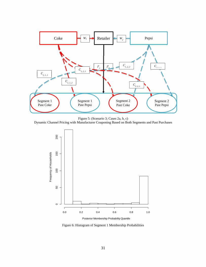
First, we simulate the channel members’ profits under the assumption that the same price is

offered to both consumer segments, i.e., Scenario 1 (see Figure 1). The simulated retail and wholesale

prices, as well as corresponding retail and manufacturer profits, are reported in the second column of

Table 4. In this simulation, we employ the Empirical Bayes procedure of Kamakura and Russell (1989),

which uses the estimated heterogeneity distribution as a prior, and the complete purchase history of each

household as data, in order to classify each household in to one of the two estimated segments. Using this

procedure, we obtain posterior segment membership probabilities that are close to 1 for the assigned

segments for almost all of the households in the sample (see Figure 6 for the histogram of these

membership probabilities, which is clearly bimodal). In order to compute channel members’ profits, we

use the Pakes and McGuire (1994) algorithm. We forward simulate retail and wholesale prices for

19

multiple future periods until the prices (and the associated demands) reach steady state. We ignore cost

shocks in the simulation. For details regarding the simulation, see the Appendix.

[Insert Figure 6 here]

Next, we simulate the channel members’ profits under the assumption that the retailer mails

customized coupons to customers based on their segment membership, i.e., Scenario 2, Case 1 (see Figure

2). Again, we apply the Pakes and McGuire (1994) algorithm for this purpose, treating the values of the

customized coupons as additional control variables (in addition to the wholesale and retail prices). We

find that it is optimal for the retailer to target segment 2, which is the more price-sensitive segment, with

price-off coupons. The simulated retail and wholesale prices, retail coupon values, as well as

corresponding retail and manufacturer profits, are reported in the third column of Table 4. Comparing the

channel members’ profits in columns 2 and 3, we find that the retailer and Pepsi both benefit (with their

profits increasing by 4.8 % and 6.8 %, respectively), while Coke hurts (with its profit decreasing by 1.6

%), from the retailer’s ability to offer different retail prices to the consumer segments. This finding

slightly departs from the findings in Besanko, Dube and Gupta (2003) and Pancras and Sudhir (2007) that

both manufacturers benefit from BPD by the retailer (however, neither of those studies account for the

role of demand inertia and, instead, assume myopic pricing by channel members). We also find that the

total channel profit increases by 4.5% due to BPD by the retailer.


Next, we simulate the channel members’ profits under the assumption that the retailer mails

customized coupons to each customer based on not only their segment membership but also their most

recent purchase (which reflects the effect of inertia), i.e., Scenario 3, Case 1 (see Figure 4). The simulated

retail and wholesale prices, retail coupon values, as well as corresponding retail and manufacturer profits,

are reported in the third column of Table 5. Comparing the channel members’ profits in columns 2 and 3

of Table 5, we find that the retailer and Pepsi both benefit (with their profits increasing by 10.2 % and 5

%, respectively), while Coke hurts (with its profit decreasing by 3.3 %), from the retailer’s ability to offer

different retail prices to the consumer segments. The total channel profit increases by 6.5 % due to BPD

20

by the retailer. Comparing these changes to their counterparts in Table 4 (discussed in the previous

paragraph), we find that the retailer more than doubles their incremental profit from price discrimination

(10.2 % improvement in Table 5 versus 4.8 % in Table 4) by also exploiting the previous purchase

information of each customer in addition to their segment membership. In other words, price

discrimination over time is as important as, if not more important than, price discrimination across

customer segments. This is a new finding to the literature on BPDv and implies that a substantively

significant increase in retail profit could accrue at little to no analytical cost since tracking the most recent

purchase outcome of a customer is very easy from a database management standpoint for a retailer.


Next, we simulate the channel members’ profits under the assumption that both manufacturers,

rather than the retailer, mail customized coupons to customers (which requires us to additionally assume

that the retailer shares its customer database with the manufacturers), again under two information

conditions, one which relies on segment membership only (i.e., Scenario 2, Case 2c), while the other

additionally relies on the most recent purchase (i.e., Scenario 3, Case 2c). From a practical standpoint,

such customized couponing can be undertaken by manufacturers directly mailing manufacturer coupons

to households, effectively bypassing the retailer in their distribution. The simulated retail and wholesale

prices, retail coupon values, as well as corresponding retail and manufacturer profits, are reported in

column 6 of Table 5. Comparing the channel members’ profits in columns 3 and 6 of Table 5, we find that

the retailer and Pepsi both benefit (with their profits increasing by a further 0.5 % and 7 %, respectively),

while Coke hurts (with its profit further decreasing by 10.7 %), when both manufacturers jointly engage

in BPD, as opposed to the retailer doing BPD on its own (i.e., Scenario 3, Case 1). In other words, the

retailer can simply outsource the data analytics and customization of coupons to the two manufacturers

and improve its profit beyond what it can achieve by proactively engaging in analytics and customization

on its own!

In order to study whether it would be worthwhile for the retailer to freely share its customer

database with one manufacturer only, but not the other, so that only one manufacturer drops customized

21

coupons, we simulate channel members’ prices and profits under the assumption that (i) Only Coke drops

customized coupons, i.e., Scenario 3, Case 2a, and (ii) Only Pepsi drops customized coupons, i.e.,

Scenario 3, Case 2b. The simulation results for these two cases are reported in columns 4 and 5 of Table

5. We find that the retailer’s profits under both of these cases are lower than in column 6 when both

manufacturers jointly drop customized coupons. In fact, the profits are also lower than those obtained

when the retailer does BPD on its own (i.e., Scenario 3, Case 1). In sum, it is better for the retailer to


one manufacturer only or with neither.

We next explore whether the above implications change if the retailer can charge manufacturers

for access to its customer database, that is, if retailer can serve as information brokers and sell information

to manufacturers instead of making it available for free. In order to answer this question, we figure out the

highest price that the retailer can charge each manufacturer, which represents the manufacturer’s

willingness to pay for the retailer’s customer database, under the case when both manufacturers engage in

targeted couponing (i.e., Scenario 3, Case 2c). The highest price to charge Coke is the additional profit

that Coke obtains under Scenario 3, Case 2c relative to Scenario 3, Case 2b (when only Pepsi drops

customized coupons), while the highest price to charge Pepsi is the additional profit that Pepsi obtains

under Scenario 3, Case 2c relative to Scenario 3, Case 2a (when only Coke drops customized coupons). In

other words, the retailer can charge $0.0268 (= $0.2210 - $0.1942) to Coke and charge $0.1375 (=

$0.5929 - $0.4554) to Pepsi in order to let them use its customer database. These prices can be understood

as follows: Suppose the retailer makes the following take-it-or-leave-it offer to the manufacturers: “I will

charge $0.0268 ($0.1375) to Coke (Pepsi) for use of my customer database.” If both Coke and Pepsi

accept the offer, they end up making profits of $0.2210 - $0.0268 = $0.1942 and $0.5929 - $0.1375 =

$0.4554, respectively. Suppose Coke accepts the offer, but Pepsi declines. In this case, Coke and Pepsi

make profits of $0.2862 - $0.0268 = $0.2594 and $0.4554, respectively. This leaves Coke better off, but

not Pepsi, compared to the case of both manufacturers accepting the retailer’s take-it-or-leave it offer.

Therefore, Pepsi has no incentive to decline the offer if Coke accepts the offer. Suppose Pepsi accepts the

22

offer, but Coke declines. In this case, Coke and Pepsi make profits of $0.1942 and $0.6443 - $0.1375 =

$0.5068, respectively. This leaves Pepsi better off, but not Coke, compared to the case of both

manufacturers accepting the retailer’s take-it-or-leave-it offer. Therefore, Coke has no incentive to decline

the offer if Pepsi accepts the offer. Furthermore, since $0.2594 and $0.5068 are higher than $0.1942 and

$0.4554, respectively, each manufacturer is strictly better off by accepting the retailer’s offer when its

competitor rejects the offer. This means that both Coke and Pepsi will accept the retailer’s take-it-or-

leave-it offer for access to the retailer’s customer database.

Once we account for the above, we find that the retailer will be much better off outsourcing the

customized couponing strategy to the manufacturers, with a net profit of $1.1660 ( = $1.0017 + $0.0268 +

$0.1375), which represents a 17 % increase over the profit obtained by managing BPD on its own (which

itself is 12 % higher than the profit obtained using mass market pricing, i.e., Scenario 1)! In other words,


source of business profit to the retailer. This finding is qualitatively consistent with the findings in

Pancras and Sudhir (2007), although they use a myopic pricing model in their study. Interestingly, this

yields net profits to Coke and Pepsi of $0.1942 and $0.4554, respectively, which are both lower than their

profit counterparts under Scenario 1 (see Figure 1). In other words, while the retailer benefits from

inducing manufacturers to behaviorally price discriminate by dropping customized coupons to different

customer types (which yields a profit improvement of 29 % to the retailer relative to Scenario 1, where

there is no price discrimination), it ends up making the manufacturers worse off than under the case of no

price discrimination! This is in contrast to the situation in Pancras and Sudhir (2007), where the authors

find that manufacturers’ profits improve, relative to the case of no price discrimination, along with the

retailer’s profit. This finding illustrates that information is a potent source of channel power to the

retailer in the presence of inertial demand.

Last, in order to better understand the relative importance of price discrimination over time (due

to estimated inertia effects in demand) versus price discrimination across customers (due to estimated

heterogeneity in price sensitivity), we perform a counterfactual simulation where we assume that channel

23

members rely only on the most recent purchase of each customer, and not on the customer’s segment

membership, for price discrimination purposes. We call this Scenario 4 and summarize the results of this

simulation in Table 6. In this scenario, we calculate the resulting profits to the retailer and the

manufacturers under the assumption that the retailer non-exclusively sells its customer database to both

manufacturers (which again yields the highest profit to the retailer as in Table 5). The retailer’s net profit

turns out to be $1.0405, which implies a net retail profit improvement of $0.1362 (= $1.0405 - $0.9043)

compared to the case of no BPD. In Table 5, however, the retailer’s net profit is $1.1660, which implies a

net retail profit improvement of $0.2617 (= $1.1660 - $0.9043) compared to the case of no BPD.

Therefore, BPD based only on the customer’s most recent purchase yields 52 % (= $0.1362 * 100 /

$0.2617) of the net profit gain that accrues to the retailer from BPD that simultaneously exploits the

customer’s segment membership and most recent purchase. Considering that tracking the most recent

purchase of each customer in the retailer’s data warehouse is a much easier task than calculating the

segment membership (using the customer’s full purchase history), it is remarkable that such a meaningful

retail profit lift can be obtained by using such a simple summary statistic about customer behavior. This

finding is reminiscent of the power of RFM statistics in database marketing and CRM applications (see,

for example, Fader, Hardie and Lee 2005).

Conclusions

We study behavioral price discrimination (BPD) within a distribution channel – with two

manufacturers and a retailer -- in a market with inertial demand. Using retail-level scanner panel data on

households’ brand choices, as well as weekly brand-level prices, in the cola category at a single store, we

first obtain structural estimates of consumer demand and firm pricing behavior. We use these estimates to

perform a variety of counterfactual experiments regarding BPD. Unlike previous research on BPD using

targeted coupons, which rely only on estimated differences in price elasticity across customer segments,

our structural model additionally relies on estimated differences in price elasticity across time for each

customer (that arise on account of temporal differences in the identity of the customer’s most recently

24

bought brand in the category). This, in turn, implies that our structural approach yields targeted coupon

values both across customer segments (as in existing structural models), as well as across time for each

customer segment. This allows us to understand the profit impact, for each player in the distribution

channel, of exploiting an additional source of price elasticity variation (i.e., across time) in the market.

Our key findings are as follows. First, the retailer and Pepsi both benefit (i.e., their profits

increase), while Coke hurts (i.e., its profit decreases) from the retailer engaging in BPD. Second, the

retailer can more than double their incremental profit from BPD by exploiting the most recent purchase

information of each customer in addition to their segment membership, when compared to exploiting

segment membership only. In other words, price discrimination over time is as important as, if not more

important than, price discrimination across customer segments. This is a new finding to the literature on

BPD and implies that a substantively significant increase in retail profit could accrue at little to no

analytical cost since tracking the most recent purchase outcome of a customer is very easy from a

database management standpoint for a retailer. Third, the retailer and Pepsi both benefit (i.e., their profits

increase), while Coke hurts (i.e., its profit decreases), when both manufacturers jointly engage in BPD, as

opposed to the retailer doing BPD. In other words, the retailer can simply outsource the data analytics

and customization of coupons to the two manufacturers and improve its profit beyond what it can achieve

by proactively engaging in analytics and customization on its own. Fourth, it is better for the retailer to


one manufacturer only or with neither. Fifth, if the retailer can charge the manufacturers for access to its

customer database, its profit improves by a further 17 % over the profit obtained by managing BPD on its

own (which itself is 12 % higher than the profit obtained using mass market pricing). In other words,


source of business profit to the retailer. Sixth, while the retailer benefits from inducing manufacturers to

behaviorally price discriminate by dropping customized coupons to different customer types, it ends up

making the manufacturers worse off than under the case of no price discrimination! This illustrates that

information is a potent source of channel power to the retailer in the presence of inertial demand. Last,

25

but not least, we find that BPD based only on the customer’s most recent purchase yields 52 % of the net

profit gain that results from BPD that simultaneously exploits the customer’s segment membership and

most recent purchase. Considering that tracking the most recent purchase of each customer in the

retailer’s data warehouse is a much easier task than calculating the segment membership (using the

customer’s full purchase history), it is remarkable that such a meaningful retail profit lift can be obtained

by using such a simple summary statistic about customer behavior.

Some caveats are in order. First, extending our study of BPD to additionally understand the

implications of price competition across retail stores is not only useful from a modeling standpoint, but

also may be managerially important while studying pricing in a few product categories that serve as store

traffic builders (such as laundry detergent). Second, testing the implications of our structural approach

using a controlled field experiment, where different stores undertake pricing represented by different

scenarios in our counterfactual simulations, would be a very interesting and ambitious line of research

inquiry to vindicate our key findings for retailing practice. In sum, we believe that our study has made an

important contribution to the vast literature on price discrimination by throwing light on an under-studied

dimension of behavioral pricing, i.e., price discrimination over time (charging different prices at different

purchase occasions to the same customer). This dimension acquires special significance for packaged

goods markets where inertial effects in demand are not only commonplace but significant. We show that

the profit impact of such temporal price discrimination is as meaningful as, if not more important than,

that resulting from exploiting differences across customer types.

26

References

Acquisiti, A., Varian, H. (2006). Conditioning Prices on Purchase History, Marketing Science,

24, 3, 367-381.

Besanko, D., Dube, J. P., Gupta, S. (2003). Competitive Price Discrimination Strategies in a

Vertical Channel Using Aggregate Retail Data, Management Science, 49, 9, 1121-1138.

Chen, Y. (1997). Paying Customers to Switch, Journal of Economics and Management Strategy,

6, 4, 877-897.

Chen, Y., Narasimhan, C., Zhang, Z. J. (2001). Individual Marketing with Imperfect

Targetability, Marketing Science, 20, 1, 23-41.

Cosguner, K., Chan, T., Seetharaman, P. B. (2014). Dynamic Pricing in a Distribution Channel

in the Presence of Switching Costs, Working Paper, Georgia State University.

Dube, J. P., Hitsch, G. J., Rossi, P. E., Vitorino, M. A. (2008). Category Pricing with State-

Dependent Utility, Marketing Science, 27, 3, 417-429.

Fader, P., Hardie, B. G. S., Lee, K. L. (2005). RFM and CLV: Using Iso-Value Curves for

Customer Base Analysis, Journal of Marketing Research, 42, 4, 415-430.

Fudenberg, D., Tirole, J. (2000). Customer Poaching and Brand Switching, The RAND Journal

of Economics, 31, 4, 634-657.

Iyengar, R., Ansari, A., Gupta, S. (2003). Leveraging Information Across Categories,

Quantitative Marketing and Economics, 1, 4, 425-465.

27

Kamakura, W. A., Russell, G. J. (1989). A Probabilistic Choice Model for Market Segmentation

and Elasticity Structure, Journal of Marketing Research, 26, 4, 379-390.

Liu, Y., Zhang, Z. J. (2006). The Benefits of Personalized Pricing in a Channel, Marketing

Science, 25, 1, 97-105.

Pakes, A., McGuire, P. (1994). Computing Markov-Perfect Nash Equilibria: Numerical

Implications of a Dynamic Differentiated Product Model, RAND Journal of Economics, 25,

4, 555-589.

Pancras, J., Sudhir, K. (2007). Optimal Marketing Strategies for a Customer Data Intermediary,

Journal of Marketing Research, 44, 4, 560-578.

Pazgal, A., Soberman, D. (2008). Behavior-Based Discrimination: Is It a Winning Play, and If

So, When?, Marketing Science, 27, 6, 977-994.

Rossi, P. E., McCulloch, R. E., Allenby, G. M. (1996). The Value of Purchase History Data in

Target Marketing, Marketing Science, 15, 4, 321-340.

Shaffer, G., Zhang, Z. J. (1995). Competitive Coupon Targeting, Marketing Science, 14, 4, 395-

416.

Shaffer, G., Zhang, Z. J. (2000). Pay To Switch or Pay To Stay: Preference-Based Price

Discrimination in Markets With Switching Costs, Journal of Economics and Management

Strategy, 9, 3, 397-424.

Shin, J., Sudhir, K. (2014). A Customer Management Dilemma: When Is It Profitable to Reward

One’s Own Customers?, Marketing Science, 29, 4, 671-689.

28

Taylor, C. R. (2003). Supplier Surfing: Competition and Consumer Behavior in Subscription

Markets, RAND Journal of Economics, 34, 2, 223-246.

Thisse, J. F., Vives, X. (1988). On the Strategic Choice of Spatial Price Policy, American

Economic Review, 78, 1, 122-137.

Villas-Boas, J. M. (1999). Dynamic Competition with Customer Recognition, RAND Journal of

Economics, 30, 4, 604-631.

29

Figure 1: (Scenario 1)

Dynamic Channel Pricing with No Couponing

Figure 2: (Scenario 2; Case 1)

Dynamic Channel Pricing with Retailer Couponing Based on Segments

Coke Pepsi

Retailer

Segment 1 Past Coke

Segment 1 Past Pepsi

Segment 2 Past Coke


W1 W2

P1

P2

Coke Pepsi

Retailer

Segment 1 Past Coke


Segment 2 Past Coke


W1 W2

P1, 1

P2, 1

P1, 2

P2, 2

30

Figure 3: (Scenario 2; Cases 2a, b, c)

Dynamic Channel Pricing with Manufacturer Couponing Based on Segments

Figure 4: (Scenario 3; Case 1)

Dynamic Channel Pricing with Retailer Couponing Based on Both Segments and Past Purchases

Coke Pepsi

Retailer

Segment 1 Past Coke


Segment 2 Past Coke


W1 W2

P1 P

2 P

1 P

2

C1 2

C2 2

Coke Pepsi

Retailer

Segment 1 Past Coke


Segment 2 Past Coke


W1 W2

P1, 1, 1

P2, 1, 1

P1, 1, 2

P2, 1, 2

P1 2 1

P2 2 1

P1 2 2

P2, 2, 2

31

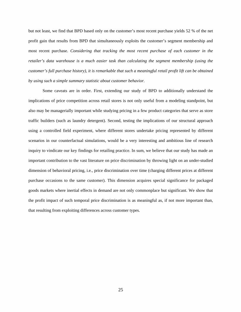
Figure 5: (Scenario 3; Cases 2a, b, c)

Dynamic Channel Pricing with Manufacturer Couponing Based on Both Segments and Past Purchases

Figure 6: Histogram of Segment 1 Membership Probabilities

Posterior Membership Probability Quantile

Fre

qu

en

cy o

f Ho

use

ho

lds

0.0 0.2 0.4 0.6 0.8 1.0

05

01

00

15

02

00

Coke Pepsi Retailer

Segment 1 Past Coke


Segment 2 Past Coke


W1

P1

P2

W2

C2, 1, 1

C1, 1, 2

C1, 2, 1

C1, 2, 2

C2, 2, 1

C2 2 2

32

TABLE 1: DESCRIPTIVE STATISTICS ON COLA DATASET1

(JUNE 1991 – JUNE 1993)

Number of Households = 356 Number of Shopping Trips = 32942

Number of Purchases = 5784

Brand Price ($ / unit) Display Feature Market Share Coke $0.8050 ($0.0680) 0.1458 (0.0953) 0.2535 (0.1249) 0.3027 (0.1038) Pepsi $0.7500 ($0.0574) 0.2236 (0.1818) 0.3314 (0.2088) 0.4567 (0.1173)

Royal Crown $0.8051 ($0.0747) 0.0943 (0.0788) 0.1067 (0.0883) 0.1721 (0.0906) Private Label $0.5311 ($0.0740) 0.1044 (0.0780) 0.0641 (0.0849) 0.0685 (0.0572)

TABLE 2: ESTIMATION RESULTS – INERTIAL DEMAND MODEL

(2-SUPPORT HETEROGENEITY)2

LL = -13716.32, BIC = 27624.15

Segment 1 Segment 2

Coke 0.950 (0.183) -0.019 (0.177)

Pepsi 1.028 (0.181) 0.136 (0.181)

PL -2.144 (0.194) -1.677 (0.138)

RoyalCrown 0.516 (0.167) -0.481 (0.166)

Price -5.233 (0.232) -6.727 (0.239)

Display 1.113 (0.078) 1.454 (0.071)

Feature 0.228 (0.078) 0.320 (0.078)

SD 1.560 (0.050) 0.858 (0.048) Size 29 % 71 %

1 Standard Deviations are reported within parentheses. 2 Standard errors are reported within parentheses in Tables 3, 4 and 5. The standard errors in Table 4 are bootstrapped standard errors.

33

TABLE 3: ESTIMATION RESULTS – DYNAMIC PRICING MODEL

Parameters Estimates Profit Margins Estimates

CokeC $0.436 ($0.025) CokeR $0.216

PepsiC $0.355 ($0.028) PepsiR $0.224

Coke $0.059 ($0.016) MCoke $0.165

Pepsi $0.073 ($0.012) MPepsi $0.197

TABLE 4: BPD COUNTERFACTUAL SIMULATION RESULTS – SCENARIOS 1 & 2

Scenario 1

(No Coupon)

Scenario 2, Case 1

(Retailer Couponing)

Scenario 2, Case 2a (Coke

Couponing)

Scenario 2, Case 2b (Pepsi

Couponing)

Scenario 2, Case 2c (Coke &

Pepsi Couponing)

CokeP $0.8319 $0.8532 $0.8410 $0.8377 $0.8479

PepsiP $0.7773 $0.7913 $0.7753 $0.7939 $0.7959

, 2Coke segCoup na $0.0838 $0.1054 na $0.1154

, 2Pepsi segCoup na $0.0926 na $0.1386 $0.1464

Cokew $0.6155 $0.6124 $0.6421 $0.6166 $0.6429

Pepsiw $0.5533 $0.5466 $0.5470 $0.5941 $0.5947

Retailer Profit $0.9043 $0.9480 $0.9354 $0.9592 $0.9694

Coke Profit $0.2557 $0.2517 $0.2808 $0.2490 $0.2708

Pepsi Profit $0.5276 $0.5633 $0.5120 $0.5999 $0.5886

Channel Profit $1.6876 $1.7630 $1.7282 $1.8082 $1.8288

Scenario 1: No targeting Scenario 2: Targeting based on segment membership only

34

TABLE 5: BPD COUNTERFACTUAL SIMULATION RESULTS – SCENARIO 3

Scenario 1

(No Coupon)

Scenario 3, Case 1



Couponing)


Couponing)


Pepsi Couponing)

CokeP $0.8319 $0.8427 $0.8896 $0.8105 $0.8885

PepsiP $0.7773 $0.7880 $0.7531 $0.8350 $0.8322

, 1,Coke seg PCokeCoup na $0.0077 na na na

, 1,Coke seg PPepsiCoup na na $0.1800 na $0.1428

, 2,Coke seg PCokeCoup na $0.0935 $0.1558 na $0.1499

, 2,Coke seg PPepsiCoup na $0.0843 $0.1811 na $0.1726

, 1,Pepsi seg PCokeCoup na $0.0159 na $0.2317 $0.2222

, 1,Pepsi seg PPepsiCoup na Na na na na

, 2,Pepsi seg PCokeCoup na $0.1120 na $0.2557 $0.2492

, 2,Pepsi seg PPepsiCoup na $0.1028 na $0.1708 $0.1683

Cokew $0.6155 $0.5960 $0.6807 $0.6166 $0.6852

Pepsiw $0.5533 $0.5386 $0.5303 $0.5941 $0.6288

Retailer Profit $0.9043 $0.9965 $0.9671 $0.9824 $1.0017

Coke Profit $0.2557 $0.2473 $0.2862 $0.1942 $0.2210

Pepsi Profit $0.5276 $0.5539 $0.4554 $0.6443 $0.5929

Channel Profit $1.6876 $1.7978 $1.7087 $1.8208 $1.8156

Scenario 3: Targeting based on segment membership and most recent purchase

35

TABLE 6: BPD COUNTERFACTUAL SIMULATION RESULTS – SCENARIO 4

Scenario 1

(No Coupon)

Scenario 4, Case 1



Couponing)


Couponing)


Pepsi Couponing)

CokeP $0.8319 $0.8299 $0.8688 $0.8176 $0.8489

PepsiP $0.7773 $0.7658 $0.7597 $0.8031 $0.8020

,Coke PPepsiCoup na $0.0191 $0.1211 na $0.0916

,Pepsi PCokeCoup na $0.0057 na $0.1901 $0.1888

Cokew $0.6155 $0.6089 $0.6807 $0.6166 $0.6852

Pepsiw $0.5533 $0.5388 $0.5303 $0.5941 $0.6288

Retailer Profit $0.9043 $0.9532 $0.9313 $0.9350 $0.9649

Coke Profit $0.2557 $0.2555 $0.2713 $0.2024 $0.2123

Pepsi Profit $0.5276 $0.5154 $0.4772 $0.5825 $0.5429

Channel Profit $1.6876 $1.7241 $1.6799 $1.7199 $1.7202 Scenario 4: Targeting based on most recent purchase only

i This is our modification of the term “behavior-based price discrimination” coined by Fudenberg and Tirole 2000 for price discrimination based on past purchase behavior. ii The cost shocks are set to zero for our all counterfactual studies in order to be able to obtain the long-run average equilibrium retail and wholesale policies. iii Substantive insights gleaned from our empirical analysis remain similar when the heterogeneity specification is modified to include additional supports for the heterogeneity distribution. These results are available upon request. iv We ignore the strategic aspect of the prices of Royal Crown and the Private Label. This can be rationalized by the observation in Table 1 that they have much smaller market shares than Coke and Pepsi and are, therefore, unlikely to significantly influence the wholesale and retail prices of Coke and Pepsi. v At first blush, it may appear that Besanko, Dube and Gupta (2003) have a similar finding when they find that exploiting the most recent purchase of a customer yields more than half the incremental profit gained from exploiting the full purchase history of the customer. However, in their case, the most recent purchase only serves as an imperfect proxy for the full purchase history while calculating the household’s price sensitivity. In our case, the most recent purchase is directly informative of the household’s price sensitivity on account of inertia effects in demand.

behavioral price discrimination in a distribution...

Documents