behavior of three metallic alloys under combined axial … · nasa/cr--2001-211162 behavior of...
TRANSCRIPT

NASA/CR--2001-211162
Behavior of Three Metallic Alloys UnderCombined Axial-Shear Stress at 650 °C
Jason E Colaiuta
Pennsylvania State University, University Park, Pennsylvania
Prepared under Cooperative Agreement NCC3-597
National Aeronautics and
Space Administration
Glenn Research Center
October 2001
https://ntrs.nasa.gov/search.jsp?R=20020009763 2018-08-20T02:10:12+00:00Z

Acknowledgments
First and foremost, I want to thank my thesis advisor, Dr. Cliff Lissenden for all of his assistance and guidance
throughout the course of this project. Also, I want to thank Dr. Bradley Lerch of NASA Glenn Research Center
for his guidance throughout the experimental portion of this project. I also want to express my gratitudefor the financial support of the NASA Glenn Research Center provided under Cooperative Agreement
NCC3-597. Furthermore, I must acknowledge everyone that I worked with at NASA GRC for the
technical support they provided. In addition, I would like to thank the members of my thesis
reading committee, Dr. Charles Bakis and Dr. Francesco Costanzo for reviewing my thesis.
Trade names or manufacturers' names are used in this report for
identification only. This usage does not constitute an officialendorsement, either expressed or implied, by the National
Aeronautics and Space Administration.
NASA Center for Aerospace Information7121 Standard Drive
Hanover, MD 21076
Available from
National Technical Information Service
5285 Port Royal Road
Springfield, VA 22100
Available electronically at http://gltrs.m'c.nasa.gov/GLTRS

Table of Contents
Section Page
List of Tables .................................................................................... v
List of Figures ................................................................................... vi
Chapter 1: Introduction ........................................................................... 1
1.1 General Introduction and Objectives ............................................. 1
1.2 Plasticity Theory ..................................................................... 21.2.1 Yield Functions .......................................................... 2
1.2.2 Loading Criteria ......................................................... 41.2.3 Flow Laws ............................................................... 5
1.2.4 Hardening Laws ......................................................... 6
1.2.5 Distortional Hardening ................................................. 7
1.3 Overview of Viscoplasticity ...................................................... 11
1.3.1 Thermodynamic Basics of Unified Viscoplasticity ............... 111.3.2 State Law ............................................................... 12
1.3.3 Dissipation Potential ................................................... 13
1.3.4 GVIPS Unified Viscoplasticity Model .............................. 141.3.5 The Bodner Partom Model ........................................... 16
1.4 Yield Surface Experiments ........................................................ 17
1.4.1 The Definition of Yielding ............................................ 181.4.2 The Yield Surface ...................................................... 20
Chapter 2:2.1
Experimental Methods ............................................................. 29Materials ............................................................................. 29
2.1.1 Haynes 188 .............................................................. 292.1.2 316 Stainless Steel .................................................... 30
2.1.3 Inconel 718 ............................................................. 31
2.2 Test Specimen ....................................................................... 31
2.2.1 Specimen Dimensions ................................................. 31
2.2.2 Specimen Preparation .................................................. 32
2.3 Test Equipment ...................................................................... 332.4 Strain Controlled Load Paths ...................................................... 35
2.5 Yield Loci ............................................................................. 36
Chapter 3:3.1
3.2
3.3
3.4
3.5
Data Analysis ......................................................................... 44
Mathematical Representation of Yield Surfaces ............................... 44
Yield Surface Representation ....................................................... 46
Parameter Determination for the Voyiadjis Model ........................... 47Goodness of Fit Statistics ........................................................... 50
Yield Surface Fitting Methodology ................................................ 51
NASA/CR--2001-211162 iii

Chapter 4:4.1
4.2
4.3
4.4
4.5
4.6
4.7
4.8
Results and Discussion .............................................................. 57
Yield Surface Data .................................................................. 57
Effect of Load Path Cycling ........................................................ 59Strain Path I .......................................................................... 60
Strain Path I/ ......................................................................... 62
Strain Path m ........................................................................ 63
Additional Inconel 718 Strain Paths .............................................. 64
Summary of Experimental Results ................................................ 65Parameter Evolution .................................................................. 65
Chapter 5:5.1
5.2
Conclusions and Future Work ...................................................... 98
Conclusions .......................................................................... 98
Future Work ........................................................................... 99
References .......................................................................................... 101
Appendix A: Catalog of Yield Surface Data ................................................. 107
Appendix B: Yield Surface Fit Parameters ................................................... 142
NASA/CR--2001-211162 iv

List of Tables
Table
2.1
2.2
2.3
2.4
A.I
B.1
B.2
B.3
B.4
B.5
B.6
B.7
B.8
B.9
B.10
B.I1
Page
Chemical Composition of Tested Materials ........................................ 30
Mechanical Propertied of Tested Materials .......................................... 30
Dimpling torque ........................................................................ 32
Yield surface probing stress rates .................................................... 37
Specimen dimensions and test matrix .............................................. 109
Haynes 188, Path I, HYII-89 ........................................................ 145
Haynes 188, Path II, HYII-86 ....................................................... 146
Haynes 188, Path HI (First Run), HYII-90 ........................................ 147
Haynes 188, Path 1II (Second Run), HYII-82 ..................................... 147
316 Stainless Steel, Path I, 610-01 .................................................. 148
316 Stainless Steel, Path II, 610-04 ................................................. 149
316 Stainless Steel, Path HI, 610-05 ............................................... 150
Inconel 718, Path I, IN-16 ........................................................... 151
Inconel 718, Path II, IN-23 ........................................................... 151
Inconel 718, Path m, IN-27 ......................................................... 152
Inconel 718, Path IV, IN- 11 ......................................................... 152
NASA/CR--2001-211162 v

List of Figures
Figure
1.1
1.2
1.3
1.4
1.5
1.6
2.1
2.2
2.3
2.4
2.5
2.6
3.1
3.2
3.3
3.4
Page
Relative difference between yield surfaces predicted by
von Mises and Tresca yield criteria ................................................ 23
The effects of isotropic and kinematic hardening on an initial
yield surface ........................................................................... 24
Change in curvature of the backside of a yield surface due to
an axial prestrain ...................................................................... 25
Change in curvature of the backside of a yield surface due to
an axial prestrain with added cross effects ....................................... 26
Difference between the direction of the strain rate and stress rate
during a strain controlled nonproprotional loading .............................. 27
Yielding definitions used in yield surface experiments ......................... 28
Specimen geometry, 2-inch specimen and 1-inch specimen ................... 39
Axial-Torsional test machine and MTS 458 analog controller ................ 40
Gripped 1-inch specimen with mounted biaxial extensometer
and induction heating coils ........................................................ 41
Strain controlled paths, (a) pure axial Path I, (b) pure shear Path II,
(c) combined axial-shear Path llI ................................................. 42
Additional In 718 strain paths, (a) Path IV, (b) Path V, (c) Path VI ......... 43
Example of probing order after a torsional prestrain ........................... 44
HN 188 Path 1I, Point C, Cycle 1 showing how the intersection of
two lines between yield points gives the center of probing ................... 54
Size change of a yield surface with changing a ................................. 55
Distortion of a yield surface with changing d ranging from 0.0 to -0.2 ..... 56
Distortion of a yield surface with changing d ranging from 0.0 to 0.01 ..... 57
NASA/CR--2001-211162 vi

4.1
4.2
4.3
4.4
4.5
4.6
4.7
4.8
4.9
4.10
4.11
4.12
4.13
4.14
4.15
4.16
4.17
4.18
4.19
4.20
4.21
4.22
Stress-Strain, (a), and Offset Strain-Axial Strain, (b), response for
an individual yield probe .......................................................... 69
Initial yield surface for SS 316 showing model fit and parameters .......... 70
Initial yields surfaces for HN 188, SS 316, IN 718 ............................ 71
Examples of HN 188 yield surfaces .............................................. 72
Examples of SS 316 yield surfaces ............................................... 73
Examples of IN 718 yield surfaces ............................................... 74
Cyclic evolution of HN 188 at selected points ................................. 78
Cyclic evolution of SS 316 at selected points .................................. 76
Cyclic evolution of IN 718 at selected points ................................... 77
Strain paths produced by Path I, (a), Path II, (b), and Path Ill, (c) ........... 78
Axial Stress-Axial Strain response for Path I .................................... 79
Voyiadjis model parameter evolution for HN 188, Path I, HYII 89 ......... 80
Voyiadjis model parameter evolution for SS 316, Path I, 610-01 ............ 81
Voyiadjis model parameter evolution for IN 718, Path I, IN-16 ............. 82
Shear Stress-Shear Strain response for Path II .................................. 83
Voyiadjis model parameter evolution for HN 188, Path II, HYII-86 ......... 84
Voyiadjis model parameter evolution for SS 316, Path II, 610-04 ........... 85
Voyiadjis model parameter evolution for IN 718, Path 11, IN-23 ............ 86
Axial Stress-Axial Stress and Shear Stress-Shear Strain responsefor Path Ill ............................................................................ 87
Voyiadjis model parameter evolution for HN 188, Path I_, HYrl-90 ....... 88
Voyiadjis model parameter evolution for HN 188, Path l/I, HYI-82 ....... 89
Voyiadjis model parameter evolution for HN 188, Path IIIfor runs 1 and 290 ................................................................... 90
NASA/CR--2001-211162 vii

4.23
4.24
4.25
4.26
4.27
4.28
4.29
4.30
A. 1
A.2
A.3
A.4
A.5
A.6
A.7
A.8
A.9
A. 10
A. I1
A.12
A.13
A. 14
A.15
Voyiadjis model parameter evolution for SS 316, Path lII, 610-05 ........... 91
Voyiadjis model parameter evolution for IN 718, Path HI, IN-27 ............ 92
Voyiadjis model parameter evolution for IN 718, Path IV, IN-11 ............ 93
Evolution of a versus plastic work for HN 188 .................................. 94
Evolution of a versus plastic work for SS 316 ................................... 95
Evolution of a versus plastic work for IN 718 .................................... 96
Evolution of all versus stress times total strain squared ....................... 97
Evolution of aj2 versus stress times total strain squared ........................ 98
Haynes 188, Path I, Points A-I, Cycle 1, HYII-89 ............................ 111
Haynes 188, Path I, Point C-I, Cycle 2, HYII-89 .............................. 112
Haynes 188, Path II, Points A-E, Cycle 1, HYII-86 ........................... 113
Haynes 188, Path 11, Points F-H, Cycle 1, HY-[I-86 ........................... 114
Haynes 188, Path II, Points B-E, Cycle 2, HYII-86 ........................... 115
Haynes 188, Path II, Points F-I, Cycle 2, HYU-86 ............................. 116
Haynes 188, Path II, Points B-E, Cycle 3, HYII-86 ........................... 117
Haynes 188, Path II, Points F-I, Cycle 3, HYU-86 ............................ 118
Haynes 188, Path Ill, Points A-F, Cycle 1, HYII-90 .......................... 119
Haynes 188, Path lII, Points B-F, Cycle 2, HYU-90 .......................... 120
Haynes 188, Path l/I, Points A-F, Cycle 1, HYII-82 .......................... 121
Haynes 188, Path l/I, Points B-F, Cycle 2, HYII-82 .......................... 122
316 Stainless Steel, Path I, Points A-E, Cycle 1,610-01 ..................... 123
316 Stainless Steel, Path I, Points F-I, Cycle 1,610-01 ...................... 124
316 Stainless Steel, Path I, Points B-E, Cycle 2, 610-01 ...................... 125
NASA/CR--2001-211162 viii

A.16
A.17
A.18
A.19
A.20
A.21
A.22
A.23
A.24
A.25
A.26
A.27
A.28
A.29
A.30
A.31
A.32
A.33
316StainlessSteel,PathI, PointsF-I, Cycle2, 610-01....................... 126
316StainlessSteel,PathI, PointsB-E,Cycle3,610-01..................... 127
316 StainlessSteel,PathI, PointsF-I, Cycle3, 610-01....................... 128
316StainlessSteel,PathII, PointsA-E, Cycle 1,610-04.................... 129
316StainlessSteel,Path1/,PointsF-I, Cycle 1,610-04..................... 130
316StainlessSteel,PathII, PointsB-E,Cycle2, 610-04..................... 131
316StainlessSteel Path1I,PointsF-I, Cycle2, 610-04....................... 132
316StainlessSteel.PathII, PointsB-E,Cycle3, 610-04..................... 133
316StainlessSteel.PathII, PointsF-I, Cycle3,610-04...................... 134
316StainlessSteel PathffI, PointsA-F, Cycle 1,610-05.................... 135
316StainlessSteel,PathffI, PointsB-F, Cycle2, 610-05.................... 136
316StainlessSteel PathIll, Points B-F, Cycle 3,610-05 .................... 137
Inconel 718, Path I, Points A-I, Cycle 1, IN-16 ................................. 138
Inconel 718, Path I, Points C-I, Cycle 2, IN-16 ................................. 139
Inconel 718, Path II, Points A-I, Cycle 1, IN-23 ................................ 140
Inconel 718, Path 11, Points A-I, Cycle 2, IN-23 ................................ 141
Inconel 718, Path m, Points A-D, Cycle 1 ....................................... 142
Inconel 718, Path IV, Points A-E, Cycle 1 ....................................... 143
NASA/CR--2001-211162 ix


Chapter 1
Introduction
1.1 General Introduction and Objectives
Structural components used in aero-propulsion applications are often subjected to
complex multiaxial stress states while at high temperatures. Under such demanding
conditions materials can incur permanent deformations and changes in material state.
When faced with such a difficult situation the engine designer would be greatly aided by
a viscoplasfic multiaxial deformation model that could accurately describe the material
response over a wide range of conditions. Viscoplastic models such as the GV/PS
developed by Arnold et al.[15] or Bodner-Partom [18] models can perform this task.
Unfortunately, these models have yet to be validated under complex service conditions.
This is due to the fact that experiments used for validation must subject the material to
multiaxial stress states as well as elevated temperature. In short, the testing is very
complex, expensive, and time consuming.
The work presented here is an extensive study of the evolution of yield surfaces
after axial-torsional prestraining. It consisted of two phases, the experimental research
conducted at NASA Glenn Research Center (NASA-GRC), and data analysis conducted
at Penn State University. The goals of the study were: (1) build a library of yield surface
data for Inconel 718, Haynes 188, and 316 stainless steel, (2) mathematically fit the yield
NASA/CR--2001-211162 1

surface data with a model incorporating yield surface distortion effects, and (3) use the
model parameters to construct evolution equations describing the yield surfaces.
1.2 Plasticity Theory
Classical plasticity is a mathematical theory that describes permanent time-
independent deformation of materials, such as metals at room temperature. Such
mathematical theories are phenomenological in nature and are based on experimental
observations. Classical plasticity theories have three distinct parts, a yield criterion, a
plastic flow rule, and a hardening rule. The current section will discuss these three topics
as well as loading criteria and will then introduce viscoplasticity.
1.2.1 Yield Functions
Yield functions are used to separate elastic stress states from those where plastic
deformation occurs. For an isotropic metal under isothermal conditions the general form
of the yield function can be written as,
f = F(crij ) - k = 0 (1.1)
where F(cij) is a function of the current stress state and k is a constant based on the initial
tensile yield strength of the material. Yielding initiates when f=0 and the surface defined
by this condition is know as the yield surface. All stress states inside of the yield surface
are elastic and stress states outside of the yield surface are not permitted unless a
viscoplastic model is being used. As a result, the yield surface must evolve as plastic
deformation occurs in order to insure that the stress state remains on the yield surface.
NASA/CR--2001-211162 2

Thetwo mostpopularyieldingcriteriaareassociatedwith Tresca[1] andvon
Mises[2] criteria. Bothof thesetheoriesarefor isotropicmaterialsandaredeviatoricin
nature.
TheTresca,or maximumshearstresscriterion isbasedon theassumptionthat a
material will yield if the maximum shear stress exceeds the critical shear strength, Tr,.
The critical shear strength is defined as "rr = (_r/2 where Cry is the tensile yield strength.
In terms of the principal stresses the Tresca yield condition takes on the following form,
f = max_al- °,,I,1o,,- o,,,I,1o,,,-o,1)-o, (1.2)
where 01, c11, azll represent the principal normal stresses and _v the tensile yield strength.
Equation 1.2 assumes a fully three-dimensional stress state, however the work in this
study involves only stress states in the axial-shear stress plane. Consequently, there are
only two non-zero stress terms: axial stress, (_11, and shear stress, (_12. Therefore, the
Tresca yield function reduces to,
61"1+ 4°1"-' = °r (1.3)
The Tresca yield criterion is very easy to apply, however it often provides a conservative
estimate of the yield stress.
The von Mises yield criterion often agrees better with experimental results than
the Tresca criterion. This criterion is also known as the distortion energy criterion
because it predicts yielding to occur when the maximum distortion energy exceeds the
energy required to cause yielding under pure tension. The von Mises theory can be
expressed as,
f= 3_2-6 r =0 (1.4)
NASA/CR--2001-211162 3

whereJ2 is the second invariant of deviatoric stress given by,
1
J= =2sijs,j (1.5)
and deviatoic stress, sis, is defined as,
1
sij = o'ij - -362 6ij (1.6)
where 56 is a second order identity tensor.
the von Mises yield criterion becomes
all + 3tYj-2 = O'r. (1.7)
Figure 1.1 shows the relative size of yield surfaces predicted by the Tresca and von Mises
yield criteria. Also note from Esq. 1.7 that if the shear stresses are multiplied by _/3 the
yon Mises ellipse becomes a circle. This characteristic will be used extensively in later
analysis.
1.2.2 Loading Criteria
In order to discuss plastic flow it is first necessary to present a formal definition
of loading. There are three different types of loading that can occur in a work hardening
material when the stress state is located on the current yield surface. If an infinitesimal
stress increment is added to the stress state directed outside of the yield surface then the
loading condition becomes,
f=0 and Of dry o > 0. (1.8)0cri i
However, a stress state located outside of the yield surface is not permitted therefore the
yield surface must evolve to accommodate the new stress state.
When expressed in the axial-shear stress plane
NASA/CR--2001-211162 4

Thesecondloadingconditionisonewherethestressincrementis directedsuch
thatit movesthecurrentstressstateinsideof the yield surface. This is called unloading
and is given by,
f--0 and Of do.ij < 0. (1.9)0% '
The final loading type is called neutral loading, which occurs when the
infinitesimal stress increment is directed tangent to the yield surface. This type of
loading causes no evolution of the yield surface and can be represented by
f=O and _f do'_j =0. (1.10)_¢r;j
1.2.3 Flow Laws
As already stated, when a material reaches a stress state where f=0 it ceases to
behave in a linear elastic manner and incurs permanent deformations. Because of this
permanent deformation the material is said to undergo plastic flow. This plastic flow
changes the material state, which drives the evolution of the yield surface. Since plastic
strain is path-dependent, it must be computed in an incremental form, deij.
It is often convenient to define the flow law in terms of a plastic potential function
such as the one presented by von Mises [3],
bf2de,] = d_ (1.11)
_o'_j
where _ is a plastic potential function that is a scalar function of stress, d_ is a
nonnegative scalar that is zero unless the stress state is on the yield surface and the
It can be shown that _f2_ is normal to the plastic potential/o _Yij
loading criteria is satisfied.
NASA/CR--2001-211162 5

function,_, thereforetheplasticstrainincrementis alwaysnormalto theplasticpotential
function. Consequently, Equation I. 11 is known as the normality flow rule.
If the potential function in Equation I. 11 is a yield function then the flow law
becomes an associated flow law. If the yon Mises yield criterion is used (Equation 1.4)
then Equation 1.11 is known as the Prandtl-Reuss flow law (Prandtl [4] and Reuss [5]),
given by,
dei_ = dAsij. (1.12)
1.2.4 Hardening Laws
Hardening occurs when the conditions in Equation (1.8) are met. Since the stress
increment tries to push the stress state to fall outside of the yield surface the surface must
evolve. This evolution is called hardening. There are three types of hardening that are
relevant to this study. They are isotropic, kinematic, and distortional hardening.
Isotropic hardening occurs when the yield surface increases in size without a change in
shape or translation of the center point. This type of hardening implies an overall
increase in the yield strength of the material. In contrast, kinematic hardening is a change
in the location of the center of the yield surface without a change in size or shape. The
Bauschinger effect results from kinematic hardening. Figure 1.2 shows changes in the
yield surface due to isotropic and kinematic hardening effects. Distortional hardening is
more difficult to represent mathematically than the other two types. It is a change in the
overall shape of the yield surface. This often involves a change in the curvature of the
yield surface, usually an increase in the front and a decrease in the back. An example of
curvature change after an axial prestrain is shown in Figure 1.3. Another distortional
NASA/CR--2001-211162 6

effect is knownasacrosseffectwhich is achangein thesizeof theyield surfacenormal
to thedirectionof prestraining.Positivecrosseffectsareshownin Figure 1.4.
A general yield function, such as the one in Equation 1.1 can be easily altered to
incorporate isotropic hardening effects. This is accomplished by making k a function of a
state variable q that accounts for the material loading history. As the total plastic strain
imparted on the material increases, k(q) increases, resulting in an overall increase of the
material yield strength in all loading directions.
The yield function in Equation 1.1 can also be altered to represent kinematic
hardening as follows,
f = F(tyij -a_i )- k (1.13)
where t_ij is known as the back stress tensor. The back stress describes the translation of
the yield surface with respect to the plastic deformation history of the material. Note that
k is a constant.
It follows that these two hardening types can easily be incorporated into a single
model to describe both isotropic and kinematic hardening as shown,
f = F(ty;j -aij ) - k(q) (1.14)
This mixed hardening model often better predicts yield surface evolution than either of
the previous two, however, it still does not account for any change in the shape of the
yield surface.
1.2.5 Distortional Hardening
Being a change in shape, distortional hardening is not easily described
mathematically. The change in shape is greatly influenced by the direction of loading. In
NASA/CR--2001-211162 7

order to discuss distortional hardening, a preloading direction must first be defined. The
direction of the plastic loading is known as the preloading direction and dictates the
nature of the distortional effects seen in the subsequent yield surface. Figure 1.3 shows
yield surfaces with a tensile preloading direction.
An important point is that the prestrain and prestress directions are not always
coincident. This is particularly true for nonproportional loadings. For example, let a
specimen be loaded in tension into the plastic regime under strain control. If loading is
then continued, under strain control, in the shear direction the stress will not follow the
same path as the strain. Once shear straining is initiated the axial stress will begin to
reduce due to plastic coupling effects. However, the axial strain does not change when
shear strain is applied. This is illustrated in Figure 1.5, where figure (a) shows the strain
path followed while figure (b) shows the response of the stress. The arrows show the
direction of the change in stress at the given point.
There have been many approaches used to describe distortional hardening effects.
One approach, by Ortiz and Popov [6], uses trigonometric functions. The yield function
that they used is,
f=Is,,ll-o,0+ cos=0.+ cos 0,)
where Ilsijll is the norm of the effective deviatoric stress defined as _,ij = (sij - (Xij), (_y is the
initial tensile yield strength, P2 and 133 are model parameters that describe cross effects
and changes in curvature respectively, and 02 and 03 give the angle between the effective
deviatoric stress tensor and the phenomenological internal variables 132and 133. These
internal variables are unit tensors that define the direction of the yield surface
NASA/CR--2001-211162 8

characteristicbeingmodeledby thatterm. Forexample,sincethetermwith subscripts3
representdistortion,[33would representthedirectionin whichthedistortionoccurs.This
modelhastheability to representisotropic,kinematic,anddistortionalhardening,
howeverthemodelparametershavelittle physicalmeaning.
AnothermodeldevelopedbyEisenbergandYen [7] usesa secondordertensorto
describedistortioneffects. Theyield functionfor thismodelis,
f: l(si/-o_ij + Ri;Xsij-aij + &/)-k 2 (1.16)
where Rij is a tensor that describes distortion. The model was shown to accurately
reproduce isotropic, kinematic, and distortional hardening effects. The parameter Rij
models both distortional and isotropic hardening of the yield surface. The rate equation
/_iJ = -_ui/ (1.17)
for Rij is,
where uij is a unit tensor describing the direction of distortion and _, describes the
magnitude of distortion.
the initial yield stress.
Zyczkowski and Kurtyka [8-10] constructed a model to describe yield surface
distortion based on geometric arguments. The foundation of the model is based on the
ability to describe a closed surface from two circles with different radii and center
locations. The model is given by,
(1.18)
Isotropic hardening is handled by defining Rij as proportional to
NASA/CR--2001-211162 9
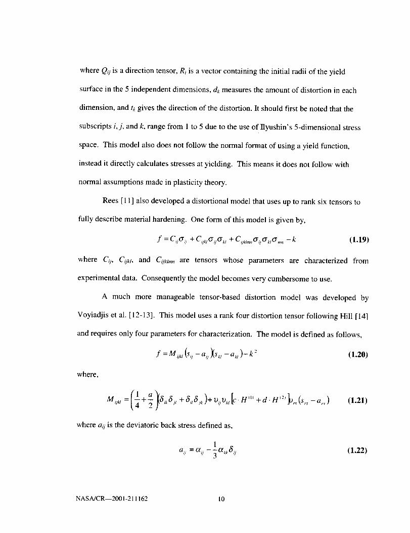
where Q;j is a direction tensor, Ri is a vector containing the initial radii of the yield
surface in the 5 independent dimensions, dk measures the amount of distortion in each
dimension, and tt gives the direction of the distortion. It should first be noted that the
subscripts i,j, and k, range from 1 to 5 due to the use of Ilyushin's 5-dimensional stress
space. This model also does not follow the normal format of using a yield function,
instead it directly calculates stresses at yielding. This means it does not follow with
normal assumptions made in plasticity theory.
Rees [ 11] also developed a distortional model that uses up to rank six tensors to
fully describe material hardening. One form of this model is given by,
f = Cijcrij + Cijkt(:rij(Ykl + Cijklmnl_ij(_'kl(_rnn -- k (1.19)
where Cj, Cijkt, and Cijklm,, are tensors whose parameters are characterized from
experimental data. Consequently the model becomes very cumbersome to use.
A much more manageable tensor-based distortion model was developed by
Voyiadjis et al. [12-13]. This model uses a rank four distortion tensor following Hill [14]
and requires only four parameters for characterization. The model is defined as follows,
: : M _jk,(s,j - a,, Xsk, - ak, )- k _- (1.20)
where,
1,4 2 'krJ' +Si'rJk)+ViJVa'[c'H'" +d'H¢2_}o'_(s"s-ar_)
where aij is the deviatoric back stress defined as,
aij = _ij --lat,.k (_ij
(1.21)
(1.22)
NASA/CR--2001-211162 10

In the model, a is a parameter defining isotropic hardening, c and d define front and back
distortion respectively. The tensor vii is a unit tensor providing the preloading direction,
where a unit tensor is given by [[_ij[[ = 1. Furthermore, _ and/__2) represent Heaviside
functions which are defined as,
H"' = H(t_ (s,., - a,., ))
H '2' =H(-v,.,.(s,.-OC,))
where the Heaviside function is defined as,
H(x)={lo ififX>0x<0
(1.23)
(1.24)
This model has the capability to be linearized which makes it very useful to for this work.
This feature allows the model parameters to be found using linear regression. This
process will be discussed further in section 3.3.
1.3 Overview of Viscoplasticity
Time-dependent material response can occur in nearly all structural materials, but
it is especially important at elevated temperatures. As a result, a model used to describe
deformation in time-dependent material must be able to handle the effects of phenomena
such as creep and stress relaxation. Models based on classical time-independent
plasticity often have separate equations for time-independent and time-dependent strains.
Making them seem like completely unrelated mechanisms. However, unified
viscoplasticity models attempt to include all permanent deformations into a single
inelastic strain term. The following sections briefly discuss the thermodynamic
NASA/CR--2001-211162 11

framework that can be used to develop viscoplasticity models. Two viscoplasticity
models are then summarized.
1.3.1 Thermodynamic Basics for Unified Viscoplasticity
Elastic and inelastic deformations in materials can also be thought of as reversible
and irreversible processes. From this, the material response can be represented in a
thermodynamic framework. When constructing a viscoplasticity model from
thermodynamic arguments the basic principals must be obeyed.
• Conservation of Mass
pdV = constant (1.25)
where p is density and dV is an infinitesimal volume element.
• Conservation of Linear Momentum
SRpb_dV + S_Rcr_jn_dS = [.Rpa,dV (1.26)
where b are body forces, a are accelerations, dS is an infinitesimal area, and nj are
the components of a unit vector normal to the surface.
• Conservation of Angular Momentum
_RPeijk xj b_dV + [._Re_#x i a_ n_dS = _i_Peijk xj a kdV (1.27)
where xj is a position vector and eikl is the permutation tensor.
• Conservation of Energy
pfa = crije ij + pr - qi._ (1.28)
where u is the intemal energy density, r is heat supplied, and qi, i heat flux.
• Clausius-Duhem Inequality
NASAICR--2001-211162 12

.2,,where _ is the specific entropy and T is the absolute temperature.
1.3.2 State Law
In viscoplasticity the material state is more complex to define than in rate-
independent plasticity. It is common to not only define the stress state (cYij), but also the
absolute temperature (73 and an array of internal variables (_) to characterize the
material state. Note, _ can be a combination of vectors and tensors. The thermodynamic
potential is given by the Gibbs free energy,
G = <yije_j - H (1.30)
where H(¢ij, T, _a) is the Helmholtz free energy given by,
H = u- Ts (1.31)
where u is the specific internal energy and s is the specific entropy. The Gibbs free
energy can be differentiated to give the following,
dG OG da_i + _G dT OG- + _b_,, (1.32)
such that,
aG aG aG
"_ij = Oaij S OT P'* 04,, (1.33)
where pc, is a generalized force term. From this the total strain rate is given by,
d[ _G)= ()2G _2G T _2G(124)
Under isothermal and linear elastic conditions the second and third terms go to zero.
NASA/CR--2001-211162 13

1.3.3 Dissipation Potential
With the material state defined it is now possible to derive a flow law for
viscoplasticity. In rate-independent plasticity the flow law was written in terms of a
plastic potential function. Here a similar potential function is used, called the dissipation
potential, f2((_ij, 7", _._). As a result the flow law can be written as,
af_• in __
eiJ 0o'_j (1,35)
It is clear from this definition that the dissipation potential evolves as inelastic strain is
accumulated. The evolution equation can be expressed in terms of the internal state
variable such that,
0QP,, - (1.36)
a(,,
where p,_ is the first derivative ofp_ with respect to time. When isothermal conditions
are considered, Equation( i .29) can be given in terms of the Gibbs free energy,
P,_- 02G _. (1.37)
1.3.4 GVIPS Unified Viscoplasticity Model
The Generalized Viscoplasticity Model with Potential Structure (GVIPS),
developed by Arnold et al. [ 15-17], provides a good example of a model derived from the
method discussed in section 1.3.1-1.3.3. This model uses a yield criterion, one internal
variable (back stress, _j), and an evolution law to account for nonlinear hardening.
For the GVIPS model the Gibbs free energy is given by,
NASA/CR--2001-211162 14

ill
G=G E +G, +G a =--2Cqk, GqCrk, --Gqeq -Bo(g + B,g p) (1.39)
_ mis the inelastic component of strain. The dissipation potential is,where eq
.,/f n+ 1 -- q+l_ + R,_B o8 (1.40)
n+l q+l
For the GVIPS model the internal state variable is the back stress, ctij, which has the
conjugate Aij. The model is governed by three basic equations: the flow law,
el;""' =/_Eij (1.41)
the evolution law,
Qqkl Cklpq b pq
Jtij =bij
and the internal constitutive rate law,
where
. in • in
2J2
Lqk_ = Q-_i_t= K_ (Iqk_ + K2aijak_ )
• i _ K3aob_ = eq
3a6a U
2,¢o
(1.42)
(1.43)
(1.44)
(1.45)
(1.46)
(1.47)
(1.48)
NASA/CR--2001-211162 15

1J_ = -:-ZijZ;, Z;s (1.49)- 2 _ = s_/- aii.
In the above equations,f is the yield function, y defines the stress below which only
elastic strain exists, I0k_ is the fourth order identity tensor, Zij is the effective stress, Jz is
the second invariant of deviatoric stress, and ( ) are the MacCauley brackets, defined as,
if,_ o(x)-- . l.SO ifx >0
The constants K_, K2, and K3 contain the model parameters (Bo, Bl, R,_, Xo, x, fl, n, p, q).
1.3.5 The Bodner Partom Model
The Bodner-Partom model (Bodner and Partom [18-19]) is presented as an
example of a viscoplasticity model that does not follow a thermodynamic framework.
Instead the model is based on dislocation dynamics and no formal yield function is used.
The Bodner-Partom model allows inelastic strains under any loading condition.
However, there are many loading conditions where the inelastic strain is insignificant
compared to the elastic term. A basic outline of the model is provided below, for more
information see Bodner and Partom [18].
The total strain rate is first broken down into an elastic and inelastic part,
"e
eij = e;3 + e_ (1.51)
• e "in
where e;j and e;j are the elastic and inelastic strain rates, respectively. The elastic strain
rate is given by the time derivative of Hooke's law and the inelastic strain rate is given by
the Prandtl-Reuss flow law (Equation 1.12). In this case the constant _ accounts for
isotropic hardening and is given by,
NASA/CR--2001-211162 16

= Do (1.52)
Z: " 17+1)]- L[ 3J2 ) _ _1,
where Do, Z, and n are model parameters. Kinematic hardening is represented by using
an effective internal variable,
t ° t .
Ze_ = Z o + qIZ(r)dr +(l-q)r!: fZ(r)rijdr0 0
(1.53)
where
O"Ur - (1.54)
are the current stress direction cosines and the evolution equation is given by,
2 = re(z, - Z)W., (1.55)Zo
• it!
where Wi, , = ffi:eij is the inelastic power. The parameters that must be determined are
Zo, Zb Do, m, n, and q.
1.4 Yield Surface Experiments
There have been many experimental studies on the yield characteristics of metals.
In this section, an attempt is made to review previous yield surface work that most
closely pertains to the current study. Excellent review papers on yield surface
experimental studies were written by Hecker [20] and Michno and Findley [21 ].
NASA/CR--2001-211162 17

1.4.1 The Definition of Yielding
In most yield surface experimental studies the specimen of choice is the thin-
walled tube. This type of specimen can easily be subjected to various ratios of axial and
shear stress in order to map a yield surface in the axial-shear stress plane. In addition, the
specimen can be subjected to internal pressure in order to define a three-dimensional
yield surface.
When mapping yield loci there are two basic approaches. First, use a separate test
specimen for each point on the surface, or use the same specimen to map an entire yield
surface. The second approach is the most common because of the cost benefits and the
elimination of specimen-to-specimen scatter. However, when using a single specimen to
determine multiple yield points the state of the material must not change between each
probe. This leads to a careful consideration of the definition of yielding.
There are many different definitions of yielding ranging from the standard 0.2%
offset strain rule, which accumulates 2000 _te (_te = 10"6 ITl/m) of plastic deformation, to
the proportional limit definition, where there is no plastic strain accumulated. The three
most common definitions of yielding for yield surface evaluations are the proportional
limit definition, the offset strain definition, and the back extrapolation definition. Each of
these definitions can produce significantly different test results due to the sensitivity of
yield to small amounts of plastic strain. Representations of these yielding criteria with
respect to the stress-strain curve are shown in Figure 1.6.
The proportional limit criteria defines yield to occur at the point where plastic
strain begins to accumulate. This method requires very precise measurements of strain in
order to be sure that yielding is detected as the onset of non-linearity in the stress-strain
curve. Phillips et al. [22 - 25] used a version of the proportional limit definition in
NASA/CR--2001-211162 18

combination with a back extrapolation technique in order to define yielding with zero
plastic strain. The method used involves first loading until two consecutive data points
deviated to the same side of the linear elastic loading line. From here the last three points
were fit with a line and yielding was defined as the intersection of this line and the linear
elastic loading line.
The offset strain method is considerably easier to implement in experimental
investigations. However, the magnitude of the offset strain is largely arbitrary, but
different values can be required depending on material and loading rate. When used in
multiaxial experiments the offset strain is given by an equivalent offset strain, such as,
eq "_3 ij ,j 11
oZ is the offset strain tensor, and el_ and e_'_ are the axial and shear componentswhere e,_
respectively. Small offset strain values, on the order of 10 _, represent the initiation of
fielding and are nearly the same as the proportional limit definition of yielding.
However, larger offsets, such as the 0.2% offset criterion, give a macroscopic view of
fielding and overall plastic flow. Because these large values cause considerable changes
in material state the specimens cannot be used to determine multiple yield points in a
locus. As a result, small offset strains are often used in yield surface experiments. Target
offset values differ between experimental investigations. Some examples are, Helling et
al. [26-28] used 5 _te, Gil et al. [29-30] used 30 la_, and Nouaihas and Cailletaud [31]
used 100 !tt_.
The back extrapolation method is probably least used of the methods described
because it requires a material with near linear hardening characteristics. In addition, it is
NASA/CR----2001-211162 19

oftennecessaryto strainthetestspecimenwell into theplasticregionin orderto fit a
straightline. As aresult,thetestspecimenscannotbeusedfor multipleyieldpoint
determinations.This techniquewasusedby TaylorandQuinney[32] to determinethe
multiaxial yieldingbehaviorof copper,aluminum,andmild steel.
Thenextquestionwhendevelopingayield surfacetestingprogramis what
control methodshouldbeused.Thetwo mostobviouschoicesareconstantloadingrate
andconstantstrainrate. StudiesperformedbyPhillips andLu [25] andWu andYen [33]
determinedthattherewasnosignificantdifferencebetweenstress-controlledandstrain-
controlledyield surfacesfor purealuminumspecimenstestedonaservohydraulictest
machine.
Anotherconsiderationfor yield surfacestudiesis theeffectof strainrateon
yielding. Ellis et al. [34] performedastudyondependenceof probingrateon thesmall
offset yieldingbehaviorof type316stainlesssteelatroomtemperature.It wasfoundthat
for strainratesbetween100and500lardmintherewasnosignificantchangein theyield
surface.Theseresultsagreewith classicalrate-independentplasticity. However,
plasticityis alwaysrate-dependantto somedegreeandtheratedependencetypically
increasesatelevatedtemperatures.This is especiallytrueathigh stresses.Therefore,the
strainrateusedduringprobingwill play anincreasedroleat elevatedtemperature.
1.4.2 The Yield Surface
Investigations of the initial yield surfaces of metals date back to before the
aforementioned work of Taylor and Quinney [32]. Their research found that for copper
and aluminum the von Mises yield criterion more accurately described initial yielding in
NASA/CR--2001-211162 20

theaxial-shearstressplanethantheTrescacriterion. Thisconclusionhasbeenconfirmed
by manyotherresearches,suchas,Phillips et al. [22], Liu [35], andHelling et al. [26].
Theevolutionof theyield surface,asamaterialis subjectedto permanent
deformation,is alsoof interest.Whatthesesubsequentyield surfaceslook like depends
on thedefinitionof yieldingused. ff a largeoffsetis used,suchasthe 2000_tEusedby
Hecker[36], thesubsequentyield surfaceappearsto beanisotropicexpansionof the
initial yield surface.However,if a smalloffsetor proportionallimit criterion is usedthe
subsequentyield surfaceexhibitsacombinationof isotropic,kinematic,anddistortional
hardening.Experimentalwork doneby KhanandWang[37] providesastudyof the
effectof offsetstrainsrangingfrom 200to 2000/aaonyield surfaceshape.
In addition,yield surfacescanalsoexhibit substantialcross-effects.Positive
cross-effects,anincreasein thesizeof theyield surfacenormalto theprestraindirection,
werefoundin studiesperformedby Phillips andTang[23] andWu andYen [33]. In
contrast,negativecross-effects(decreasein width normalto prestraindirection)were
seenby Michno andFindley[21] in mild steels.A studyby Williams andSvensson[38]
showedthataluminumexhibitedlargecross-effectswhensubjectedto torsion
prestraining,but zerocross-effectsafteraxialprestraining.
Whenanalyzingsubsequentyield surfacesit is quickly realizedthatisotropic
hardening,kinematichardening,andcrosseffectscannotfully explainexperimental
results.Subsequentyield surfacesalsoshowconsiderableamountsof distortional
hardening.This is characterizedbeadecreasein curvatureof theyield surfacein the
directionoppositeto thedirectionof prestraining.Theyield surfacealsocontinuesto
exhibitsymmetryabouttheaxisof prestraining.Theseconclusionshavebeenfoundby
NASAJCR--2001-211162 21

many researches including Phillips et al. [22], Phillips and Moon [24], Helling et al. [26],
and Wu and Yeh [33].
NASA/CR--2001-211162 22

von MisesYield Theory
- - - Tresca Yield Theory
J //• J
///_/
/
Axial Stress
Figure 1.1: Relative difference between yield surfaces predicted by yon Mises and
Tresca yield criteria.
NASA/CR--2001-211162 23

ra_
t--
/
/
\
\
ff
1f
J
/ //
/ fiI
I
\\ \
\
r/
/i
j/
jJ_ j
jJ
J
JJ
Initial Yield Surface
Isotropic Hardening
Kinematic Hardening
\
\
\,
/ /
/
/
I
Figure 1.2:
Axial Stress
The effects of isotropic and kinematic hardening on an initial yield surface.
NASA/CR--2001-211162 24

/
/'
t
J
S
//
/
/
,,£
+t
k\
Prestrain Direction
£ •
/ /£/ I
I /' +/
/
/, ,,
_-_ tQ
\.4
I$,
J
f
/,
/
Axial Stress
Figure 1.3: Change in curvature of the backside of a yield surface due to an axial
prestrain.
NASA/CR--2001-211162 25

t19
e-
r.,¢)
'L
Prestrain D irection
I
'_r _ ,I
J-/
I S
_% •
\
f
J
J
J
/
J
©
II
/
_i_
_J
Axial Stress
Figure 1.4: Change in curvature of the backside of a yield surface due to an axial
prestrain with added cross effects.
NASA/CR--2001-211162 26

(a)
,D
e-
.A
_C
,B
Axial Strain
t,ot/"l
a,..atl)
I1)t"t.t)
(b)
Axial Stress
Figure 1.5: Difference between the direction of the strain rate and stress rate during astrain controlled nonproportional loading.
NASA/CR--2001-211162 27

®
Figure 1.6: Yielding definitions used in yield surface experiments.
NASA/CR--2001-211162 28

Chapter 2
Experimental Methods
The yield surface evolution experiments carried out for this study were complex
and tedious. The following discussion concerns the methodology used in this study to
perform yield surface evaluations and prestraining of the specimens. This chapter will
discuss the materials, test specimen, test equipment, and test procedures used. The goal
was to apply the same methodology to a wide range of materials in order to develop yield
surface evolution equations.
2.1 Materials
This study consisted of testing three materials with significantly different
compositions. The materials tested were Haynes 188, 316 stainless steel, and Inconel
718. By testing such different materials it was hoped that differences in the way the yield
surfaces evolve could be seen.
2.1.1 Haynes 188
Haynes 188 (HN 188) is a cobalt-based alloy, see Table 2.1 for the composition
given by the manufacturer. Its primary uses include nozzle guide vanes, stator blades,
and combustion liners in aero-propulsion systems. The material was tested in a solution
annealed state. In this state the microstructure contains second phase carbides that
provide an additional hardening component to the material response. The solution
annealing process was conducted as follows,
NASA/CR--2001-211162 29
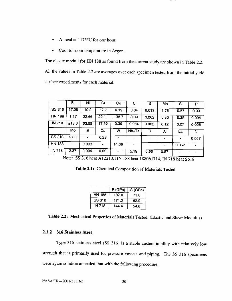
• Anneal at 1175°C for one hour.
• Cool to room temperature in Argon.
The elastic moduli for HN 188 as found from the current study are shown in Table 2.2.
All the values in Table 2.2 are averages over each specimen tested from the initial yield
surface experiments for each material.
SS 316
HN 188
IN 718
SS 316
HN 188
IN 718
Note:
Fe Ni Cr Co C S Mn Si
67.08 10.2 17.7 0.19 0.04 0.013 1.75 0.57
1.17 22.66 22.11 ±38.7 0.09 0.002 0.80 0.35
±18.6 53.58 17.52 0.39 0.034 0.002 0.12 0.07
Mo B Cu W Nb+Ta Ti AI La
2.08 0.28
- 0.003 14.06 - 0.052
2.87 0.004 0.05 5.19 0.95 0.57
P
0.03
0.005
0.006
N
0.067
SS 316 heat A12210, HN 188 heat 188061714, IN 718 heat $618
Table 2.1: Chemical Composition of Materials Tested.
Table 2.2:
E(GPa) G (GPa)HN 188 187.0 71.6
SS 316 171.2 62.9
IN 718 144.4 54.8
Mechanical Properties of Materials Tested. (Elastic and Shear Modulus)
2.1.2 316 Stainless Steel
Type 316 stainless steel (SS 316) is a stable austenitic alloy with relatively low
strength that is primarily used for pressure vessels and piping. The SS 316 specimens
were again solution annealed, but with the following procedure.
NASA/CR--2001-211162 30

• Anneal at 1065°C for 30 minutes.
• Cool to 537°C in 9 minutes.
• Furnace cool to room temperature.
The composition of SS 316 is shown in Table 2.1 and the elastic moduli in Table 2.2.
2.1.3 Inconel 718
Inconel 718(IN 718) is a very high strength nickel-based alloy. It is mainly used
in aeropropulsion applications for structural components such as disks, blades, and shafts.
IN 718 was tested in an aged state. In order to reach this state the specimens were first
solution annealed and subsequently aged. The thermal processing was conducted as
follows.
• Anneal at 1038°C for 1 hour.
• Air cool to room temperature.
• Age in vacuum at 720°C for 8 hours.
• Cool to 620°C at 55°C/min and hold for 8 hours.
• Cool in Argon to room temperature.
This heat treatment produces 7" precipitates that significantly increase the hardness of
the material. Table 2.1 shows the chemical composition of IN 718 and Table 2.2 gives
the elastic moduli.
2.2 Test Specimens
This section details the two different types of test specimen used. It also
discusses the procedure for preparing a specimen to be tested.
NASA/CR--2001-211162 31

2.2.1 Specimen Dimensions
All of the test specimens used where of the thin-walled tube type. However, two
different size specimens were used. The specimen sizes have no effect on the testing
procedure other than the physical setup of the load frame grips and geometric constants
used for interpreting the test data. Both HN 188 and SS 316 used the specimen type
referred to as the 2-inch specimen due to its two-inch diameter grip section. IN 718 is
the specimen referred to as the 1-inch specimen due to its one-inch diameter grip section.
The exact dimensions of the 2-inch and 1-inch specimens are shown in Figure 2.1.
2.2.2 Specimen Preparation
Prior to testing each new specimen needed to be dimpled in order to accept the
biaxial extensometer and fitted with thermocouples. Dimpling consisted of placing two
small indentations in the gauge section of the specimen for the extensometer probes to
rest. This was performed by using a dimpling device custom built at NASA GRC. The
equipment consisted of a base that firmly held the test specimen in place with a screw
used to lower the dimpling tool (supplied with the extensometer) to the specimen.
Torque was then applied to the screw via a torque wrench in order to dimple the
specimen. This setup allowed the same dimpling force to be applied to each specimen,
precisely controlling the size of the dimples. Table 2.3 show the dimpling torques used
for each material.
Material Torque (N'm)
HN 188 2.03
SS316 1.58
IN 718 1.81
Table 2.3: Dimpling torque.
NASA/CR--2001-211162 32

Thesecondstepin preparingthetestspecimenswasto spotweld thermocouples
to thegaugesectionof thespecimen.A totalof threethermocoupleswereappliedto
eachtest specimen.Thethermocoupleswereappliedatthecenterand 12.5mm above
andbelowcenteron thegaugesection.Thecenterthermocouplewasusedto control the
inductionheatingsystem.Theremainingtwo thermocouplesdefinedthetemperature
gradientacrossthegaugesection.
2.3 Test Equipment
All experiments in this study were conducted on a computer controlled MTS
biaxial servohydraulic test machine. The machine is pictured in Figure 2.2 and is located
in the NASA GRC multiaxial fatigue lab. The maximum capacities of the load frame are
+220,000 N axial loading and +2,260 N*m twisting moment. The test specimen is held
by water-cooled, hydraulically actuated grips. The top grip is fixed while the bottom grip
is attached to a hydraulic actuator that is capable of independent vertical translation and
rotation. Two MTS 458 analog controllers, one for axial motion and one for torsional
motion, control the actuator. Further details about the biaxial test machine are given by
Kalluri and Bonacuse [39].
Specimen heating was accomplished by using a closed-loop induction heating
system as described by Ellis and Bartolotta [40]. The system consisted of an Ameritherm
15-kW radio frequency induction heating unit and three adjustable, water-cooled copper
coils surrounding the gauge section of the specimen. The copper coils could be raised or
lowered independently along the gauge section of the test specimen in order to obtain an
NASA/CR--2001-211162 33

acceptabletemperaturegradient(+ 1% of the absolute test temperature). See Figure 2.3
for a photo of the copper coils around a 1-inch specimen.
In order to conduct yield surface studies, strain measurements accurate to the
microstrain level are required. This is because loading must be quickly stopped once
yield is detected in order to ensure the material state is not significantly disturbed. In
addition, the device used to measure strain must also perform on a micro strain level at
elevated temperatures. This depends not only on the strain measurement device, but
also on the ability of the heating equipment to maintain a constant temperature and the
elimination of electronic noise.
This study utilized an MTS water-cooled biaxial extensometer capable of
operating over a large temperature range. The extensometer used two alumina rods,
spaced 25mm apart to measure axial deformation and twist. The alumina rods fit into
the dimples placed in the test specimen as discussed earlier. Lissenden et al. [41] supply
further details on the biaxial extensometer. The biaxial extensometer mounted to a
specimen is shown in Figure 2.3.
Custom written software and a PC were used to control all experiments. The PC
was equipped with analog-to-digital (A/D) and digital-to-analog (D/A) hardware. The
D/A hardware sent a command signal from the PC to the load frame while the A/D
hardware received test data. Both sampled at 1000 Hz. The test data received by the
A/D hardware averaged the data over every 100 points in order to minimize the effects
of electronic noise, providing 10 data points per second written to output files.
NASA/CR--2001-211162 34

The test program utilized two separate control programs. One was used to
determined the yield points used to construct the yield loci while the other program
preformed the preloadings.
2.4 Strain Controlled Load Paths
All three materials were subjected to a series of three strain controlled load paths.
Path I is purely axial strain, Path 11is purely shear strain, and Path 1TI is a non-
proportional strain path. A schematic of each load path is shown in Figure 2.4. Along
each load path several stops were made in order to conduct a pair of yield surface
determinations. These points are indicated by letters in Figure 2.4. In addition, each load
path was cycled either two or three times depending on the hardening characteristics of
each material. For each load path the maximum equivalent strain is 15,000 kt_, shown by
a dashed circle in Figure 2.4.
Three additional load paths were carried out on IN 718. These paths were not
carried out on the other materials due to time constraints and the lack of success with IN
718. These additional load paths all subject the material to both axial and torsional strain.
They are designated Path IV, Path V and Path VI and are shown in Figure 2.5.
All six load paths used an equivalent strain rate of 100 _te/s. For axial-torsional
loading equivalent strain is given by,
_eq_ij_ij = _2 [(1 + 2V 2 )_1 + 2_12 ] (2.1)
where eij is the strain rate tensor, v is Poisson's ratio, and ell and e12are the tensorial
axial and shear strain rates respectively.
NASA/CR--200I-211162 35

2.5 Yield Loci
Each yield locus was constructed by probing for yielding in 16 unique directions
in the axial-torsional stress plane. The angles used for probing were identical for each
locus, however the order of probing varied depending on the prestrain history of the
material. The angles were always setup in such a fashion that the first probe was in a
direction normal to the prestrain direction. Furthermore, the order of subsequent probes
was chosen in order to minimize the changes to the material state. For example, Figure
2.5 shows the order of probing following a torsional prestrain. In this pattern, the angle
between probes was either 180 ° or 90 ° in the hopes that the effects of the probes would
counteract each other. Minimization of the changes in material state while performing
yield surface determinations is further discussed by Hecker [42]. In addition, each yield
surface was repeated to verify that the material state was undisturbed.
Each of the 16 individual yield probes can be broken down into the following
three step process,
(i) Use a least squares fit to determine the coefficients of the elastic loading
line over a predefined stress range within the elastic region. These
coefficients include the elastic modulus, E, shear modulus, G, and initial
stresses cr°t and cr°2.
(ii) Continuously calculate the offset strain components using the following
equations,
all -- (_]°l_e_°_ = e_ (2.2)
E
NASA/CR--2001-211162 36

0"12 - O'l°_el_H = e,2 (2.3)
2G
From this determine the equivalent offset strain (Equation 1.33) and
compare it to the target value of 30 _e.
(iii) Once the equivalent offset strain exceeds the target value unload the probe
to the starting position.
The 30 _t_ value for the offset strain was chosen based on previous experience
from studies performed by Lissenden et al. [43] and Gil et al. [44]. In order to obtain
optimum results with the least scatter each material used a different probing rate. Prior to
testing a material a rate study was performed in order to determine the optimum probing
rate. This was done by conducting initial yield surfaces tests for each material at various
stress rates. Multiple runs of each rate were perform and the rate that showed the best
repeatability was used as the yield surface probing rate for that material. The results of
these rate studies are given in Table 2.4.
Material
IN 718
Equivalent Stress Rate
(MeaJs)2.07
Equivalent Elastic Strain
Rate (lain/m/s)10
HN 188 17.9 100
SS 316 7.24 50
Table 2.4: Yield surface probing stress rates.
NASA/CR--2001-211162 37

(n- t -7-
1
_L j !2! _..1_._ _
,CD
,7"-1('..1
[.---- _,o
Er-e-,
oi
e-,
=_
.<
....z
O
"ra
""7
e,-
°_
e-"7t-',!
o
e.,
e4
t..,
NASA/CR--2001-211162 38

Figure 2.2: Axial-TorsionaltestmachineandMTS458 analogcontroller.
NASA/CR--2001-211162 39

Figure 2.3: Gripped 1-inch specimen with mounted biaxial extensometer and induction
heating coils.
NASA/CR--2001-211162 40

(a)Path I
d
t
/
/
/
H I
O i -F
x
Shear
Strain
x
\
\
X
A B :
4 = 6
E D _
/
t
/
Axial
Strain
(b_ Path II
s
Dt
i
¢
EI
_ F
\
Q
t Shear] Strainiic
B
A
J
I J¢
t
Ht
/
. /
Axial
Strain
tc) Pafllm
#
C, #
Shear
Strain
_ Bx
e x
/Ak1
I /
AxialStrain
Figure 2.4: Strain controlled paths, (a) pure axial Path I, (b) pure shear Path II, (c)combined axial-shear Path 1II.
NASMCRI2_ 1-211162 41

(a)Path1_7 Shear
B_A "_
E D AxialStrain
(b}PathVD
C
ShearStrain
A H
B O
Axial
Strain
(c) Path VI
C
B A
F
Shear
Strain
D
Axial
Strain
E
Figure 2.4: Additional In 718 strain paths, (a) Path IV, (b) Path V, (c) Path VI.
NASA/CR--2001-211162 42

(21q3)EA
a 9
13 al i
_,. _ ! .4
7 " "\', J_' i // _ 1_
_.... ",, II , I _,' ._'
-_-_ "" _'" "" _ 0....................... .................+
16 - _ _ ",.d -,
/' i i _i
10 : 4
(0.906)s,,
Probe Probe
Number Angle
1 12o
2 1_ °
5 102 °
4 282°5 57°
6 237 _
7 147_
8 _7 _
Probe ProOo
Number Anglei, i Ha,H .....
9 7g ='
10 259°
11 170 o
12 35O=
1:_ 125 °
14 305 °
15 35 °
16 215 Q:::::
Figure 2.5: Example of probing order after a torsional prestrain.
NASA/CR--2001-211162 43

Chapter 3
Data Analysis
The overall goal of this research was to describe the evolution of the yield surface
when subjected to plastic deformation. As a result, an integral part of the data analysis
was to find a way to describe the yield surface by a model with parameters that change
as the yield surface evolves. The first section of this chapter will discuss some of the
attempts made to find such a model. Section 3.2 will discuss how the model developed
by Voyiadjis et al. [13] and its parameters were used to reproduce yield surfaces and how
the model parameters affect its shape, size, and position. Section 3.3 will detail the steps
taken to reduce the model to an axial-torsional form that could be fit using linear
regression. Finally, Section 3.4 will discuss the statistical methods used to quantify
goodness of fit.
3.1 Mathematical Representation of Yield Surfaces
The first attempts made at fitting a shape to the yield surface data collected in
this study applied the simplistic approach of fitting a circle with a flattened backside.
The definition of the backside of a yield surface is the portion of the yield surface from
approximately 90 to 270 degrees from the prestrain direction. This initial attempt to
describe the yield surface was based on two principles; (i) the initial yield surface as well
as the front side of the yield surface are circular in the 011-_/3t_12 stress plane, (ii) the
backside of the surface flattens compared to the front and can be represented by a straight
NASA/CR--2001-211162 45

line. Thisrepresentationprovedadequatefor describingyield surfaceswith little or no
distortion,however,it quickly falteredwhenexposedto highlydistortedyield surfaces.
In addition,thebacksideof theyieldsurfaceis nota straightline evenwhensignificant
distortionis present.
Thesecondapproachinvolvedtheregressionof polynomials. Sincetheproblem
at handis highlynonlinearthepolynomialsneededto beof order2 or greater.
Furthermore,termsinvolving bothaxialandshearstressneededto be includedin order
to obtainthedistortedshapeof theyield surface.As aresult,theregressionparameter
becameverycomplex. Nonetheless,themajorshortcomingof theapproachcamefrom
thefact thatit wasnot alwayspossibleto obtaina continuoussmoothsurface.When
usedto predictayield surface,thepolynomialregressionoftenproducedacuspwhen
thecurveintersectedtheaxial-stressaxis. This wasnotconsistentwith anyof the
experimentalresultscollected.
Thepolynomialapproachwasextendedto includeconformalmapping.It was
hopedthatadataconversioncouldbefound thatwouldallow thedatato be fitted and
thenconvertedbackto its original form. This processagainproducednon-continuous
yieldsurfaces.In addition,themappingprocessincreasedtheerrorbetweendataand
fit curvesresultingin pooryield surfacerepresentations.
Finally it wasdecidedthatayield function approachwasneeded.Severalyield
functionbaseddistortionalmodelswerediscussedin Section1.2.5. Of these,themodel
developedby Voyiadjiset al. [12, 13]waschosenfor tworeason: (1) it produceda
continuousconvexyield surface,(2) all of thepertinentyield surfacecharacteristics
NASA/CR--2001-211162 46
could can be controlled by four parameters. From this point this distortion model will be
referred to as the Voyiadjis model.
3.2 Yield Surface Representation
The algorithm used to reproduce a yield surface once the model parameters were
determined did not require a reduction to the axial-torsional form. The Voyiadjis model
was used in the form shown in Equations 1.20 and 1.21 and programmed in to MathCAD.
The yield surface was predicted by incrementing stress in the same probing direction
used in the experimental portion of this study. First the program automatically found the
starting stress point for all probes. To do this, probes 1 and 2 were fit with a line as well
as probes 3 and 4. The intersection between these two lines gave the initial stress point
for probing, as shown in Figure 3.1 where C represents the center of probing. From this
point probing is carried out in all directions. This technique produced yield points in the
same directions as the experimentally determined yield points.
Each of the four parameters control a different type of hardening. The parameter
a is related to isotropic hardening. Its value does not have a bound, but a=l corresponds
to a radius equal to the initial yield strength averaged from all specimens tested, k0. Then
if a> 1 the yield surface is smaller than the initial surface and if a< 1 the yield surface is
larger than the initial surface. This is shown in Figure 3.2. The parameter d determines
the amount of distortion there is in the backside of the yield surface. A value of zero
gives no distortion, ff the value is greater then zero than the yield surface distorts with an
increase in curvature along the backside, as shown in Figure 3.3. If the value of d is less
then zero the yield surface distorts with a decrease in curvature, as shown in Figure 3.4.
The backstress parameters, _tlt and tXL2,control the location of the center of the yield
NASA/CR--2001-211162 47

angle respectively.
surface. The values of these parameters depend on the properties of the material being
tested, but they generally have an association with the maximum stress reached during
a preloading.
The value of the directional unit tensor, uij, was calculated from the prestrain
direction. Since all preloadings occurred in the axial-shear strain plane the axial and
shear proportions of the loadings could be found from the cosine and sine of the loading
If the directional tensor is given as,
where 0 is the prestrain direction.
from,
rxco 0x.sin0 i]v_i = Ix- s_n0 00
By enforcing [l_ijll= 1 the value of x can be found
(3.1)
x 2 cos 2 0 + 2x z sin 2 0 = 1. (3.2)
3.3 Parameter Determination for the Voyiadjis Model
The first step in determining the parameters for the Voyiadjis model was to
reduce it to its axial-torsional form by making the appropriate assumptions. Since the
entire set of yield surface data is in the axial-torsional stress space the stress and
backstress tensors can be reduced to,
.I ll l:!l0 0
The deviatoric stress and deviatofic backstress are,
NASA/CR--2001-211162 48

30-lJ
s(] = O"12
0
O'12 0
1-- --O'lj
30
10 --0-Jl
3
"2
a 0 = 0_12
0
0_12
1----O_ll
3
0
0
0
1-- --O_ll
3
(3.4)
One additional assumption is that the direction tensor, 1)ij, is also contained in the axial-
torsional plane giving,
1)ll Ul2 0
1) ij =" 0 .
0
(3.5)
When the above assumptions are made only 25 of the 81 components of the tensor Mijkt
(Equation 1.21 ) are non- zero. Next, Mijkt is substituted into Equation 1.20 and the
number of non-zero components furthers reduces to 11 for the completed axial-torsional
form of the Voyiadjis model.
With the axial-torsional reduction completed, work was initiated to obtain a form
that could be used with a regression technique in order to obtain the model parameters.
The problem was originally approached with the desire to obtain all four model
parameters directly from regression. However, it is assumed that the backstress follows
the same direction as the prestrain direction. As a result, it was easier to use an iterative
method to find the backstress. An initial guess was input and the value was incremented
in the direction of prestrain until the fit no longer improved. The method used to quantify
the goodness of fit will be discussed in the next section. Since the backstress was not
included in the regression the model reduced to a simple linear problem with the
following characteristic equation,
NASA/CR--2001-211162 49

r =/_okg+/_,z (3.6)
where,
2 . 4
Y = -_a(, + 2a?_ -_a,,_,_-4a,2cq, - +2a?, + 2a_2 (3.7)
Z
4 8 -, 8 8H;2I*W * O'l, Oll- _O'IIO[,,DI2 "l--_O',,O'12OllOl2---'_Gllal2OllOl2
(3.8)
(3 2 )W = o11Oll ---_ct_loit + 2o'ptgt2 -- 2aj.,o_2(3.9)
H_ 2' = H( - W) (3.10)
1
- 1+ a(3.11)
-d(3.12)
and ko is the initial yield strength averaged over all specimens of the same material tested.
Linear regression was applied to Equation 3.6 to obtain following system of equations
that can be solved by using matrix inversion,
1,o.EZ 2z 2J[B, yYZ(3.12)
where n denotes the number of probes in a yield surface. Finally Equations 3.11 and 3.12
are used to solve for a and d.
NASA/CR--2001-211162 50

The yield surface fits were produced using both repeated yield surfaces at each
point along a load path. This provided a maximum of 32 separate yield points in 16
directions for each yield surface. Prior to, fitting the data were inspected visually to
determine if a set contained outliers. A point was considered an outlier if it clearly did
not fit the pattern suggested by the remaining data points. If a point was suspected of
being an outlier fits were conducted with and without the data point and the better of the
two was accepted. Yield points were excluded on an individual basis, ff a yield point
was excluded the corresponding point in the repeated surface was not necessarily
excluded.
3.4 Goodness of Fit Statistics
The next problem was to quantify the goodness of the fit reproduced by the
outlined process. Since linear regression was used the correlation coefficient was found
to be sufficient for analyzing the fits. The experimental data and model predictions had
to first be converted to fit the form given by Equation 3.6. This was accomplished by
substituting the data and model parameters into Equations 3.7 and 3.12. The correlation
coefficient statistic in terms of Y and Z is,
Ezy.EZZ YR = n (3.12)
,/_,Z_- -,,Z2 _ _'_- -n_ _ )
where 7 and Y- are the average of all Z and Y values respectively. The value of R was
then squared to get the coefficient of determination. It is stated by Kiemele et al. [45]
that IRI > 0.7 represents a good fit. However the yield surface data did not produce R 2
values that large, but still produced good fits in the axial-torsional stress plane. The
NASA/CR--2001-211162 51

actual R 2 values range between 0.4 and 0.15. There is a correlation between R 2 and cycle
number such that the R 2 values tend to decrease in the later cycles. This is largely due to
an increase in experimental scatter in the later cycles. In addition, the fits used were not
always statistically the best fit. This is due to the assumption that d<O. All fits used were
the best fit where this assumption was satisfied.
3.5 Yield Surface Fitting Methodology
Each yield surface was fit using the same series of steps. First an initial guess for
the backstress parameters was made. This was accomplished by fitting a circle to the
front side of the yield surface and using the center of the circle as the backstress. This
worked very well for initial yield surfaces and for surfaces in the first cycle of a strain
path. However, surfaces from later cycles sometimes required the initial backstress to be
determined from experience. This was because as the distortion increased in later cycles
the backstress no longer corresponded with the center of the front side. Therefore the
initial backstress was obtain from the patterns observed in the evolution of the backstress
from the initial cycle.
Once an initial backstress was found the yield function was fit to the experimental
data. The fitting process produced the isotropic parameter, a, and the distortional
parameter, d, for a given backstress. Next, the backstress was incremented in the
direction of prestraining. Because of this iterative process it was often desirable to make
the initial guess for the backstress slightly under predict the magnitude of the expected
final backstress value. This enabled the generation of data on both sides of the optimum
fit. The best fit was the one with the largest R 2 statistic and a negative value of d.
NASA/CR--2001-211162 52

Once the best fit was obtained, it was compared to the experimental data in order
to search for possible outliers. An outlier was considered to be a yield point that did not
follow the pattern given by the other data. Outliers were determined largely by judgment.
However, if a yield point was suspected it was removed from the fit and the entire
process outlined above was conducted again. The new fit, without the outlier, was then
compared to the original. The fit that had the largest R 2 statistic was then chosen as the
fit for that yield surface.
NASA/CR--2001-211162 53

t-_
e-e-_r_
M
0.00 --
-400.00
,r
4'
r-
L
-400.00 0.00 400.00
Axial Stress fMPa)
Figure 3.1: HN 188 Path II, Point C, Cycle 1 showing how the intersection of two lines
between yield points gives the center of probing.
NASA/CR--2001-211162 54

] I L _ I
400.00 --
c._
I--i
,.c:
,-,w
0.00 --
-400.00--
a=O
a=1
a=0.5
a=2
I ' I I
-400.00 0.00 400.00
Axial Stress (MPa)
Figure 3.2: Size change of a yield surface with changing a. (ko = 203.1 MPa)
NASAJCR--2001-211162 55

400.00
m:l
*
200.00 --
0.00 --
-200.00
x_
X_
-FO
®
®
®
®
®
®
®
®
®
><_ d=0
d : -0.01
_- d = -0.1
d = -0.2
ii
-4oo.oo _ I _ I _ r-400.00 -200.00 0.00 2oo.oo
Axial Stress (MPa)400.00
Figure 3.3: Distortion of a yield surface with changing d ranging from 0.0 to -0.2.(ko = 203.1 MPa)
NASA/CR--2001-211162 56

t I i I
tl)
.-x-
100.00
0.00
-100.00
II
@ ®®
@
,9÷
@® @
®
i
®
®
®
d=O
d = 0.075
/_ d = 0.01
I _ I f I
-100.00 0.00 100.00
Axial Stress (IvIPa)
Figure 3.4: Distortion of a yield surface with changing d ranging from 0.0 to 0.01.
(ko = 84.4 MPa)
i
I
E
iL
NASA/CR--2001-211162 57


Chapter 4
Results and Discussion
With the amount of experimental data collected it is important that the results be
presented in a concise manner. It was decided that the data should be given in a format
that handled each strain path separately. This allows for comparison between the three
materials for each strain path. Section 4.1 will first introduce some of the experimental
yield surface data. Each section from there will briefly discuss the behavior of each
material for a given load path and then show summary plots of the evolution of the
primary variables. The variables of interest are a, d, all, and a12 because these are the
four parameters that describe the yield surface in the Voyiadjis distortion model. After
the three primary strain paths are discussed the additional paths applied to IN 718 will be
discussed. Note, this section does not try to present all of the yield surface data collected.
An entire set of the data and model fits can be found in Appendix A.
4.1 Yield Surface Data
All yield surface tests revolve around the ability to obtain individual yield points
from each probing direction. Therefore, it is appropriate to show details of at least one
yield probe. Figure 4.1 shows (a) the stress-strain response and (b), the offset strain-total
strain response of a 12° yield probe for HN 188. From Figure 4.1 (a) the small offset
strain is visible from the separation between the loading and unloading lines of the stress-
strain curve. Furthermore, Figure 4.1 (b) shows that the offset strain reached a value of
NASA/CR--2001-211162 59
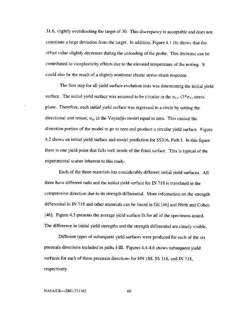
31.6,slightly overshootingthetargetof 30. This discrepancyis acceptableanddoesnot
constitutea largedeviationfrom thetarget. In addition,Figure4.1 (b) showsthatthe
offset valueslightly decreasesduringtheunloadingof theprobe. This decreasecanbe
contributedto vicoplasticityeffectsdueto theelevatedtemperatureof thetesting. It
couldalsobe theresultof a slightlynonlinearelasticstress-strainresponse.
Thefirst stepfor all yield surfaceevolutiontestswasdeterminingtheinitial yield
surface.Theinitial yield surfacewasassumedto becircularin theG11-_3"oL2stress
plane. Therefore,eachinitial yield surfacewasregressedto acircle by settingthe
directionalunit tensor,uij, in theVoyiadjismodelequalto zero. Thiscausedthe
distortionportionof themodelto go to zeroandproduceacircularyield surface.Figure
4.2showsaninitial yield surfaceandmodelpredictionfor SS316,PathI. In this figure
thereis oneyieldpoint thatfallswell insideof thefitted surface.This is typicalof the
experimentalscatterinherentto this study.
Eachof thethreematerialshasconsiderablydifferentinitial yield surfaces.All
threehavedifferent radii andtheinitial yield surfacefor IN 718is translatedin the
compressivedirectiondueto its strengthdifferential. More informationon thestrength
differential in IN 718andothermaterialscanbe foundin Gil [46] andHirth andCohen
[46]. Figure4.3presentstheaverageyield surfacefit for all of thespecimenstested.
Thedifferencein initial yield strengthsandthestrengthdifferentialareclearlyvisible.
Different typesof subsequentyieldsurfaceswereproducedfor eachof the six
prestraindirectionsincludedin paths1-111.Figures4.4-4.6showssubsequentyield
surfacesfor eachof theseprestraindirectionsfor HN 188,SS316,andIN 718,
respectively.
NASA/CR--2001-211162 60

The solid line in each figure represents the initial yield surface. From the graphs
it is clear that the kinematic hardening component of the yield surfaces follow the
prestrain direction. It can also be seen that the distortion is in the opposite direction of
the prestrain. In addition, when compared to the initial surface each subsequent surface
shows isotropic hardening. Closer inspection of the data shows that each yield surface
has two distinct parts: ( 1) a well-defined circular front side, and (2) a poorly defined
flattened backside. The front side of the surfaces encompasses the yield point within the
range of _+90° from the direction of the most recent prestrain direction. The front side is
also more-or-less centered with respect to the prestrain direction. Along the backside
of the yield surface (approximately 90 ° to 270 ° ) the curvature decreases. Significant
experimental scatter in the yield points along the backside of the yield surface was
typically observed. This scatter tended to increase as the specimen accumulated plastic
strain as it proceeded through a given load path.
4.2 Effect of Load Path Cycling
Each load path was cycled for two or three cycles. The number of cycles was
determined by when the yield surfaces stopped evolving. Each material behaved
differently when the load paths were cycled, but in general, HN 188 and IN 718 required
2 cycles and the SS 316 required three cycles for cyclic hardening to stop. In fact, IN 718
stopped evolving by the end of the first cycle, but a second was conducted to confirm
this. Figure 4.7 shows the cyclic evolution of the yield surfaces at selected points for HN
188, Figure 4.8 for SS 316, and Figure 4.9 for IN 718. From these figures it can be seen
that the yield surfaces changed the most in the first cycle. Each consecutive cycle then
NASA/CR--2001-211162 61

producedlesshardeningeffects. SS316continuedto hardenthroughall threecycles.
HN 188showedconsiderablehardeningbetweenthefirst andsecondcycles,but little
betweenthesecondandthird. As aresult,only Path1Iwascarriedout for threecycles
for HY 188.PathHandPathm werestoppedafterjust two cycles. Thehardeningof
IN718 nearlystoppedafterjust onecycle.Theyieldsurfacesfor cyclestwo virtually
overlapthosefor cycleone. In general,thenumberof cyclesneededfor theyield surface
evolutionto stopwasinverselyrelatedto theinitial yield strengthof thematerial.
4.3 Strain Path I
StrainpathI wasapurelyaxialstrainpathasshownin Figure2.4(a). Both HN
188andIN 718weresubjectedto 2 cyclesof thispathwhile SS316wascycledthree
times. In addition,timeconstraintsmadeit necessaryto conducttheyield surface
determinationfor HN 188andIN 718atonly pointsA, C, E,G, andI. (seeFigure2.4a).
Figure4.10 (a)showstheaxialstrainpathsproducedbyPathI. Only oneexamplefor
eachloadpathis shownin Figure4.10becausethestrainpathswerewell controlledand
theresultsfor all materialslook identical. All cyclesareshownandoverlap. Figure4.11
providestheaxial stress-axialstrainresponseof eachmaterialfor PathI. It clearlyshows
therelativeamountof isotropichardeningeachmaterialexhibits. Both HY 188andSS
316showacontinuousincreasein themaximumstresswhile IN 718quickly reachesa
maximumvalue. Of primaryconcernin this sectionis theevolutionof theparameters
for theVoyiadjismodel. Theparametersareshownin Figure4.12-4.14.Thedatais
presentedin theorderof theyield surfacedeterminationsalongtheloadpath. From
Figures4.13it canbeseenthatSS316hasthemostisotropichardeningbecauseit has
thelargestchangein theparametera. SS 316 is also the only material for which a
NASA/CR--2001-211162 62

becomes negative. HN 188 has the second largest change in a and IN 718 the least. For
each of the three materials a decreases the most during the first cycle and then begins to
level off. This mirrors the observations made about the cyclic evolution of the materials
in section 4.2.
The parameter d does not have a well-defined trend. Since this term measures the
distortion in the yield surface it is greatly influenced by the scatter in the data for the
backsides of the yield surfaces. The most well behaved test, from the standpoint of the
distortion parameter, d, was HY 188 Path 1 (Figure 4.12). It shows d as nearly constantly
decreasing. This indicates an increase in distortion along the backside as the load path
progressed. The other two materials show this through roughly the first cycle but then it
becomes difficult to see a trend. Most tests included a few yield surfaces that had more
distortion than those around them. These yield surfaces often showed considerable
experimental scatter and outliers that were not used in the fit.
The axial backstress component, ct_1, follows the same pattern as the axial stress.
It starts at a value of zero for the initial yield surface for both HY 188 and SS 316.
However, due to the strength differential shown by IN 719 cql has a value of-145 MPa
for the initial yield surface. After the initial yield surface, _ takes on the same sign as
the maximum axial stress obtained during the prestrain prior to a given subsequent yield
surface. In addition, ct_ increased in magnitude with each consecutive prestrain in the
same direction. The torsional backstress component, ¢t12, is not shown for Path I because
it does not evolve during the load path.
It is worth discussing here that IN 718 showed considerably more data scatter
than the other materials. The additional scatter did affect the quality of the fits that were
NASA/CR--2001-211162 63

obtained.For someof theIN 718yield surfacesthefront sidecontainedscatteraswell
asthebackside.Severalattemptsweremadeduring testingto eliminatethisproblem.
Theyield surfacesfor IN 718wererunatconsiderablylower stressratesthantheother
materials(seeTable2.4for rates). Thisdid reducethescattersomewhat,but it is present
in all IN 718yield surfaces.
4.4 Strain Path II
Strain Path II is pure shear and is shown in Figure 2.4 (b). IN 718 was subjected
to two cycles of this strain path while HN 188 and SS 316 were tested for three. Again,
IN 718 was tested only at every other point shown in Figure 2.4 (b). Figure 4.10 (b)
shows an example of the axial strain-shear strain response for this load path. The shear
stress-shear strain response for each material is shown in Figure 4.15. Figures 4.16-4.18
show the evolution graphs for the Voyiadjis model parameters for HY 188, SS 316, and
IN 718 respectively.
In general, the same observations for the evolution of the parameters a and d were
found for Path II as Path I. Parameter a again decreased as the strain path proceeded with
the same relative changes between materials as seen with Path I. The evolution of a for
HN 188 showed more scatter than for Path 1. The distortion parameter again provided no
definite trend. It again decreased at the start of the load path and then became scattered
in later cycles.
Path II involved the evolution of the torsional backstress component, _q2. It
followed the shear stress as all followed the axial stress for Path I. The axial backstress
component did not evolve during this load path, but for IN 718 it had a non-zero value for
NASA/CR--2001-211162 64

theentiretest. This is againamanifestationof thestrengthdifferential of IN 718. The
axialbackstressmaintainedaconstantvalueof-I 45MPa.
4,5 Strain Path III
Unlike Path I and Path l], Path HI subjects the test specimen to a nonproportional
loading. Points B and F follow prestrains at 45 degrees and point D follows a prestrain at
315 degrees (see Figure 2.4(c)). The axial strain-shear strain response is shown in Figure
4.10 (c). Both the axial stress-shear strain and shear stress-shear strain graphs are shown
for each material in Figure 4.19. Figures 4.20-4.24 show the evolution graphs for the
Voyiadjis model parameters for HY 188, SS 316, and IN 718 respectively. Note that
Figures 4.20 and 4.21 show repeats runs of Path ffl for HN 188 on separate specimens.
In addition, Figure 4.22 shown the two runs of HN 188 overlaid on the same graph.
All four model parameters evolved during this load path. Both a and d showed
the same response as with the other load paths. The model parameter a decreased while d
exhibited scatter and showed no real trend. The scatter in d was particularly evident with
the yield surfaces at points C and E. The distortion parameter grew large at these two
points. The yield surfaces for Path Ill showed more experimental scatter than the other
load paths. This was due to the fact that Path m imparted more plastic strain on the test
specimen per cycle than the other load paths.
The backstress terms both evolved for this load path. Again they closely followed
the movement of their stress counterparts. The axial backstress followed the axial stress
and the torsional backstress followed the torsional stress, both at a lower magnitude but
with the same sign.
NASA/CR--2001-211162 65

Unfortunately the test of Path HI on IN 718 was not completed for even one cycle.
The test specimen buckled during the prestrain between point D and E. This is likely due
to a difference in the heat treatment of the specimen used for the test. The specimen was
aged separately from the test specimens used for the other IN 718 tests. The same
procedure was followed, but at a different time. For an unknown reason the specimen
had a yield strength, in the virgin state, that was higher than the other IN 718 specimens.
It is suspected that this increase in initial yield strength also decreased the ductility of the
specimen.
4.6 Additional Inconel 718 Strain Paths
For IN 718 three additional load paths were attempted. They were created as an
attempt to gain additional data from specimens needed for other studies. See Figure 2.5
for schematics of these additional strain paths. Only Path IV was successfully carried out
for an entire cycle. The other two strain paths caused the specimens to buckle during
prestraining. The evolution of the Voyiadjis model parameters for Path IV is shown in
Figure 4.25.
4.7 Summary of Experimental Results
The materials tests provide a wide range of microstructures, compositions, and
material properties. However, the evolution of the yield surface of all three materials can
be described by a combination of isotropic, kinematic, and distortional hardening.
Therefore, it appears that the same type of hardening laws can be used to describe each
alloy. This study also has shown that distortional hardening is difficult to accurately
NASA/CR--2001-211162 66

capture experimentally. The scatter in the backsides of the yield surfaces was relatively
small for the first cycle, but became significant in later cycles. This makes it difficult to
discuss the evolution of distortional hardening parameter with any confidence. The
remaining parameters, a, al 1, and a12, are all well behaved and there is high level of
confidence in the results.
4.8 Parameter Evolution
Of the four yield surface parameters in the Voyiadjis model three have regular
patterns to their evolution. These are a, al 1, and a12. As a result, it was attempted to find
equations to represent this evolution.
This first parameter that was considered was a. It is clear that a decreases as the
material is subjected to more plastic deformation. Therefore, it is logical to assume that it
has a relationship to the plastic work where plastic work is defined as,
Wp = O'ijei_. (4.1)
When a was plotted versus plastic work the relationship proved to be of an exponential
nature. Because a is not always positive there was a problem fitting an exponential
equation to the data. To eliminate the problem the data was shifted by adding the
absolute value of the largest negative value of a to the data. Figures 4.26-4.28 show the
results of exponential fits for each material. For each fit all of the experimental data from
each load path was used. The equations of the lines and R 2 statistics for each material are
as follows,
1. HN188
a = 1.185 * e -°°4°4_ R 2 = 0.421 (4.2)
NASA/CR--2001-211162 67

2. SS316
a = 1.021 * e -°°555wp R 2 = 0.465 (4.3)
3. IN 718
a = 0.7664 * e -°'°155_' R 2 = 0.7340 (4.4)
The back stress parameters were more difficult to fit to evolution equations. This
was because during each load path the sign of the backstress alternated several times. As
a result it was necessary to use the sign function to define the evolution of the backstress.
The sign of the stress at a given point was taken while the magnitude of the backstress
w'as related to the equivalent total strain. This relationship was used because the sign of
the backstress was always the same as the stress, but its magnitude increased as total
strain increased. Figures 4.29 and 4.30 show the results of this procedure for HN 188 and
the evolution equations obtained are,
oq_ = 113.18+3.19Z-0.035Z 2 + 0.00084Z 3 + 3.22.10-6Z 4 (4.5)
a,_, = -67.53 + 3.33Y + 0.89Y" - 0.0011Y 3 - 7.86.10 -6 y4 (4.6)
where,
The R 2 statistics for Equation 4.5 and 4.6 are 0.79 and 0.33 respectively.
(4.7)
NASA/CR--2001-211162 68

-Z
<
o
c_
E
O
Figure 4.1:
200.00 L
(a)
160.00
120.00
80.00 --
40.00 --
0.00 i
-400.00
L I
/ .
,/'
! ' ] [ 1
0.00 .400.00 800.00Axial Strain {microstrain
Loading
Unloading
i
1200.00
40.00
30.00
20.00
10.00
J
(b)
, i [ i I i i i
/ \
_.00
/
, \/
/\
/
/"
/
/,,j
Loading ]
- Unloading
0.00 , [ , : i
200,00 400.00 600.00 800.00 1000.00
Axial Strain (microstrain)
Stress-Strain, (a), and Offset Strain-Axial Strain, (b), response for an
individual yield probe.
NASA/CR--2001-211162 69

r_
<.+,_
N
r
200.00 t
I
J
0.00
-200.00
I
Point A
a = 0.8359
d=0.0
R^2 = 0.375
L , J 1 J i
/
-_- Yield Surface Run I
<_/_ Yield Surface Run 2
j , j I j-200.00 0.00 200.00
Axial Stress (MPa)
ii
Figure 4.2: Initial yield surface for SS 316 showing model fit and parameters.
NASA/CR--2001-211162 70

400
¢..q¢*'b
-_ 0
¢J3
-400
/,/
/
,/
\\
//-j
f F..
"\
/ ¸ \
S
\ //J
b
//
J
J
/ /
/ /
///,
, I
SS 316
HN 188
IN 718
Figure 4.3:
J
J
/
I
-400 0 400
Axial Stress (MPa)
Initial yields surfaces for HN 188, SS 316, IN 718.
(Averaged over all specimens tested.)
NASA/CR--2001-211162 71

L.'!
i
• 400 i
I , t , i
_a) Path I, Point C
o+ ©+ ,_
/_., +, \
/" + 0 _,
/
_ ¢
I I
-400 0
Axial Stress ib'l Pa)
,_. F _
I
4O0
400
0_
-400 [
I I _ I I
(b) Palh I. Point G
<> + ?
@ +© /@ _,, /
I [
-400 0
Axial Slress (btPa)
I
400
I [ I
Ic) Path II, Point C
400
-400
©fi \ ÷
I
-400
I
0
Axial Stress (MPa)
[
400
r
] I i
] (d) Pah II, Point F
t
-400
_<__._+>+ b
@4, _'
[ I
-400 0
Axial Stress {MPa)
[
400
aoo
-400
, I
(e) Path III, Point B
+
+O O 0-
-- _ 0
o _© .=
400
[ k I J
if) Path Ill, Point D
o
i o <y
,@
qa
r
-400
4 1 I i
0 400 -400 0
Axial Stress (MPa) Axial Stress _MPa)
I
aoo
Figure 4.4: Examples of HN 188 yield surfaces.
NASA/CR--2001-211162 72

i
-200 --t
200
-200
200
-200
J I , t
ial Path I, Point C
L
k-
t 2t --
.2"
-200 0 200
Axial Stress (NPa)
to) Path If, Poinl C
g,a..
.=
, I _ I J t ,i
(b) Path 1, Point G/
20{)
0 --
-200
+_ ,
%, "---+-C/__o <v
I i :
-200 0 200
Axial Stress (MPa)
200 -
0
-..200 -
{dt Path II. Point G
o+ ÷
I I I
-200 0 200
Axial Stress (MPa)
le) Path 111, Point F
O+ _ q_'_ _'oo<>+ a,a..
- _ 0-
<) :
+ _© ._
-200 -
i I I ' I
-200 0 200
Axial Stress (NPa)
Ift Path 111, Poinl D
I I I _ ! I I
-200 0 200 -200 0 200
Axial Stress (MPa) Axial Stress (MPa)
Figure 4.5: Examples of SS 316 yield surfaces.
k-i
L
I
k
I
NASA/CR--2001-211162 73

l I
I000 ia_ PaLIh L Point (
i
500
O-
-500 -
, J L I
+
+ + ,:2
/ \ + ,_
+ / +
++ ]_+ _
ir { I
-Iooo .5oo o .ioo
,4.xial Stress (M Pa I
Io00
](10(I
500
-500
i
.1ooo
-IO00
I , I
_b! Path 1, Point (}
, I
+
: +)++
+
+ +
i I !
._oo o 500
Axial SIress (blPa_
soo
-500
-IO00 !
-1000
_cl ' I J ,Path II. Point C _
+ +++-- +
+ +
[ i
!
' 1 I
-500 0
Axial Slress iMPal
tO00
- 500,:2
O--
-500 -
Fi
I ' J -I000
500 I000 -I000
, J L J , IEd_ Path 11, Point E
! 'b
\,,\ Q
0 <>
C' <>©
©00
I I I t
-500 0 500
Axial Stress qMPai
..2
IOOO
500
1 I 1 ,(e) Path I11, Point B
+ + +
++
+
4-
+
+
-SO0 - _ it--
r-IO0O _ I I i
-I000 -500 0 500 iO00Axial Stress (MPa)
Figure 4.6: Examples of IN 718 yield surfaces.
!
i
I000
I000
NASA/CR--2001-211162 74

4O0
-400 1
400
-400
400
-400
I [ , Llai Path 1, Point C"
O O<02+ O <>
!"-V <> 'k+ oc>
\_, ,) 4- 0/÷ 0
I
L
1:5i -
LI
iii
400
-400
I L
{_h) Path L Point G
I L I
'_'++ / O+A ",
o+ I' 7@+/o4- _1O_
8_+
[ [ i [ I
-400 o 400 .400 o 400
Axial Sb'ess (MPa) Axial Stress (MPa)
qc) Path II. PointIC
!
-400
I I i I
400 --
O--
-400 --
(d) Path II, Point G
oo_ _'o_+ , _+ <7_o
oo_ + +_,
I I [ t I
o 400 -4oo o 400
Axial Stress (MPa) Axial Stress (MPa)
I L
ilel Path III. Point B
I J [ _ I , I [
i {fl Path IIl. Point D
i
_ _ _oo-<> ©
°o .'_ .',l+_ _f_ / +++ ) -¢>0- i +-o
4? ,'_o _ __,, <x.-L
-"" ° *o# _+on-+ 2, o
-400 --
I r I I I I I
-400 0 400 -400 0 400
.axial Stress (MPa) Axial Stress IMPa)
Figure 4.7: Cyclic evolution of HN 188 at selected points.
NASA/CR--2001-211162 75

i J L i /
qa_ Path I, Point C r
200 ?i 0 ! -
'_ _¢_ + oo,o 0 _5 + 0 O
:_---s+ + + A¢,,,o i _
c, %o8°
-200 i
I I [ i
-200 0 20O
Axial Stress IMPat
} I , ]
Ib) Path l, Point G
ZOO 10 '25": 'C,
°_ _+2_"I_++ ....,,
:oo 1 %
-200 0
Axial Stress IIM Pab
I
200
v
-2
20O
-200
I ' _ I I
I,zl Path II, Point C 1
o _ "4-+ _'_;
I r I
-2f}0 o 200
Axial Stress tMPa)
J
_'of) _ id } Path II. Pont G
I , I
-200 q
I
__©CO / ^
v+ + L_ -t"0
oo_%00o%:,_0 © _, 0 _
[
-200
]
0
Axial Stress IMPal
[
200
L
r-
m
.g
,o,Pa'th,,,Li°,; i o 9 _. I, . _ _0 0 !
l ,o ° v_o_-_! * %--_+++ 2°1 .{
°- % + ¢;e. °s
t I _ I
-200 o 200
Axial Slress IMPa_
200
o_
-200 I
(fl Path IIlL Point D
, [
I
-200 0 200
Axial Stress iMPa)
Figure 4.8: Cyclic evolution of SS 316 at selected points.
NASA/CR--2001-211162 76

1000
500 --
-500
-1000 f
-t000
J L
ta) Path 1. Point C
I i I i
I I !
-500 0 500
Axial Stress dqPa b
I0O0
1000
500
-500
-I000
-I000
I i L
Icl Path I1. Point C
e. '_ '___
o_ /_4_ +0/
o+( 4- I
' O- /\ ,'
I000 ]_00
7 0_
-500
-1000 .
-1000
I0O0
-500
4
] i I ' -I000
-500 0 500 I000 -I000
Axial Stress (MPap
J [ , I L I , I
(bl Path l, Point G
I I I
-500 0 SO(F
Axial Stress tblPal
, t t I ,
qD) Path lI, Poinu G
] J
I000
/ © \,
+ Jo+ /
©+ +0
0
-sOl 0
Axial Stress tMPal
I
500 ] O00
-_- Cycle 1
Cycle 2
0 Cycle 3
Initial YleFd Surface
]
Figure 4.9: Cyclic evolution of IN 718 at selected points.
NASA/CR--2001-211162 77

ioooc oo
r
o_--
-20OOOOO
-2CXX__
, I, I
(al Path I, HN 188
I I I
1cooo oo oct too_ o¢
Axial Str,ll_ _ _ m ,m
20000 J ] i
tbiPathlI. SS 316
10000
I I I
.IO00D
-20000
. I , I ,
-20000 -10000 0 10000
Axial Strain (pro/m)
20000
I , ! L
qCt Path IIl, HN 188
• I ,
•;oo_ oo I I i
-20000 O0 - 1COco O0 o oo iocc¢ oo
Figure 4.10: Strain paths produced by Path I, (a), Path II, (b), and Path m, (c).
NASA/CR--2001-211162 78

<
i I i L
tai HN 188
8ooo_ I I I
20o0o00 Ioooooo o oo toooo oo
_lalSlraln q pm_m
400
-400
-20000
I L _ [ J
Ib_SS 316
I ' I I '
-IOOOO 0 I0000
Axial Strain (pmlm)
!
I
20000
-gg_
<
I000
500 --
0 -
-500 -
-I000
-20000
I , J , I J ] ,
(c) IN 718
I [ [
-I0000 0 I0000
Axial Strain (pm]m)
20000
Figure 4.11: Axial Stress-Axial Strain response for Path I.
NASA/CR--2001-211162 79

¢--O.
0O
co0)k--
4.,,a
_t3
._ C
O
200.00
0.00
-200.00
O.OOE+O
-I.OOE-3
-2.00E-3
1.00
0.00500.00
0.00
J
Ii
-500.00
0.020.00
-0.02 1
//<
//
//
/'
//
, f r E ' ' '
A C E G I C E G I
Position Along Load Path I
Figure 4.12: Voyiadjis model parameter evolution for HN 188, Path I, HYII 89.
NASA/CR--2001-211162 80

t_
t"
Q.
t_
I,nI1)k..
4..ata_
t_
x
m
._ e--
I ,4=a
t_U3
O!-
200.00
0.00
-200.00
O.OOE+O-l.OOE-2
-2.00E-2 /
1.00_
0.00
-I.00
400,000.00
-400.00
0.02
do.oo
-0.02
f\. j ',,
J
f
//
i../
', /
\ /' \
'\
\,
/,/
/
r r ' I ' F ' I _ABCDEFGH IBCDEFGH IBCDEFGH I
Position Along Load Path I
Figure 4.13: Voyiadjis model parameter evolution for SS 316, Path I, 610-01.
NASAJCR--2001-211162 81

('0
C-
Q.
"o
(.h
t
(j')
tO.I
i
•_ c
_ (./'}0I--
400.000.00
-400.00
O.OOE+O-2.00E-1
-4.00E-1
1.00
0.001000.00
0.00 1
-1000.00
0.02 ---1
0.00
-0.02
J \ //
// \, j"\ / \, /
\\,,
'\
,i ¸/-
/,
\\,,zJ j"
f,
x/
/"
/,, /
IA C
' I ' i ' i IE G I C E G I
Position Along Load Path I
Figure 4.14: Voyiadjis model parameter evolution for IN 718, Path I, IN-16
NASA/CR--2001-211162 82

200
-2C0
-20000
I I ' I
-I0000 0 I0000
ShearStrainlum/ml
20000
20O
I00 -
0--
[
-I00
-200
L
{bl SS 316
I I
-I0000 0
Shear Slrain I I_mem
]I
I0000
800 I L
tel IN 718
400
-400 t
-800 |
-20000
L I , I
I F I ' I
-10000 0 I0000
Shear Strain (pm/m)
20000
Figure 4.15: Shear Stress-Shear Strain response for Path II.
NASA/CR--2001-211162 83

tl}(-CI.
"I=I
t_
tD
,,i.a
{.Dk..
(D¢.-
el3
L
(1) e'-r'-'_
tn_
O
200.00
0.00
-200.00 _
O.OOE+O
-1.00E-3 _
-2.00E-3 _
1.00 -_
0.00 /
400.00
0.00
-400.00_
0.02
0.00-0.02
//
\\\ /
'\ /'\ / ', /,
F
AB CDE FGH I B CDE FGH I B CDE FGH I
Postion Along Load Path II
Figure 4.16: Voyiadjis model parameter evolution for HN 188, Path 11, HYII-86.
NASA/CR--2001-211162 84

t--
it'}tt}
I...l..a
1...
f_(1)
t-"Ct3
(1) ¢"r-'_
_tt).ca
O
100.000.00
-100.00O.OOE+O
r
-1.00E-2 _
-2.00E-2
1,00 -
0.00 _
-I.00-j
200.00 10.00
-200.00
0.02 1
0.00
-0.02
//
/,4¸,,¸
F -I
/ , ,,
/ // i'
\ !
E _ I ' I ' i ' IAB CD E FGH I B CD E FGH I B CD E FGH I
Postion Along Load Path II
Figure 4.17: Voyiadjis model parameter evolution for SS 316, Path II, 610-04.
NASA/CR--2001-211162 85

•_ 200.000.00r-
I-200.00-120.00
ip
-140.00(-.
-160.00 _
O.OOE+O-o -4.00E-3
-8.00E-3
1.00
0.00
u_ i000.00-_0.}
0.00('o
t-u') -1000.00
0.02to
m _ 0.00_m0
I-- -0.02
\
_'_-_ . / _ -
\.
I I _ I I I
Postion Along Load Path II
Figure 4.18: Voyiadjis model parameter evolution for IN 718, Path II, IN-23.
NASA/CR--2001-211162 86

g
v
x
<
I000
8_ooo
800 O(J
.2000000
L t L r
Ia) H N 188
[ r F r
-1000000 O_
A
_2
a=
I i
10o000o 20000(
4.00 --
0
-400
-20000
(b) SS 316
, I L t ,
! ) I
- 10000 0 10000
Axial Strain (IJm/m)
I-i
20000
2O0
-200
-200110
200
100 --4
-I00
-200
(a)HN 188
r i .
[ )
• 10000 0
Shear Strain ( _amtmt
I i
(b) SS 316
-10000 0
Shear Strain I umtm)
i
/F
I0000 20000
I0000
-I000
I i
(c) IN 718
! , I!
_oo -1 (c_ IN 718
J0"3
r
20000
-4.0O
77/ //
) ' ; I / _ f
- 20000 - 10000 0 10000 - 10000 0
Axial Strain (umlmb Shear Strain (_m/m)
I
I
I0000
Figure 4.19: Axial Stress-Axial Stress and Shear Stress-Shear Strain
response for Path 111.
NASA/CR--2001-211162 87

200.00 -_
--_'=< 0.00-200.00
---- 400.00
,- 0.00 -d,
-400.00
0.00 -_
"_ -0.01
-0,01 --_
1.00
0.00 _:
-I.00 -_
_ 4.00E+2 _
m _ O.OOE+O
oI-- -4.00E+2 --
1000.00
0.00
-1000.00
_- 0.01 !
_.____.
o.oom_rlo
-0.01
_ 0.02
X ,I
--'_orUm_ 0.00 tt-- -0.02
jJ
..../
'\, \,,
\\ f , y\\
' I ' I 'A B C D E F B C D E F
Postion Along Load Path II
Figure 4.20: Voyiadjis model parameter evolution for HN 188, Path m, HYII-90.
NASA/CR--2001-211162 88

--_= 200.00_- 0.00
-200.00
---- 400.00
.=< 0.00-400.00
0.00
-o -0.01
-0.01
0 ii°i-1,00
4.00E+2
tO
¢-.
m _ O.OOE+O
I-- -4.00E+2
_--_m"-_omm__mlO00"O00'O0
I- -1000.00
_ 0.01ooo
0
F-- -0.01_
__.._._ 0.02 1
-- _ 0.00
0
I- -0.02, j r j _
A B C D E F B C D E F
Postion Along Load Path II
Figure 4.21: Voyiadjis model parameter evolution for HN 188, Path Ill, HYII-82.
NASA/CR--2001-211162 89

--_ 200.00
_= 020 --"
=" 4
-200.00
----_ 400.00
•= 0.00
.<-400.00
0.00i
"o -0.01
-o.ol -j
1.00_
0.00
-1.00
4.00E+2
v O.OOE+O
_ _-4.00E+2
_ _ooo.oo
_ o.oo
-i000.00
.- o.o 1_ _ o.oo
-0.01
_,_.._.__0.02 ]
_ o.oo
VO-" -0.02
J jtJJ J
A B C D E F B C D E F
Postion Along Load Path II
Figure 4.22: Voyiadjis model parameter evolution for HN 188, Path m for runs 1 and 2.
NASA/CR--2001-211162 90

--_= i00.00
.= 0.00___<
-i00.00
___ 200.00.= 0.00
<-200.00
0.00-o -0.04
-0.08 _
1.00 -_l
0.00I
-1.00 _
2.00E+2 34b O.OOE+O
--u')
F- -2.00E+2
--.-_m 500.00
000,,,l.,a
o_- -500.00
.c 0.01 1_ o.oo-0.01 --
--_,.c._-0.02 1
-- _ 0.00_(.P).I--'oI- -0.02
\\
\_,//
'L /
, //
/%,,/ ',, /,' ',,, /
/ '\ /, /'// ', /'
'v'
//
/
',,v,/
, ,; 7\ //
"\"L\,,\ "%" /' "\ '" '
// \
\ /' .....,,,,, ,,, " ",,i k /
/ \ ',,
,,, ......./ '\ /
,%A _ /1%,¸ ',
_.,'/ "v"
,/ , , ,
' I ' 1 ' i _ IA B C D E F B C D E F B C D E F
Postion Along Load Path II
Figure 4.23: Voyiadjis model parameter evolution for SS 316, Path m, 610-05.
NASAJCR--2001-211162 91

--_ 200.00 ---= 0.00
<-200.00
--__ 500.00.= 0.00
< i-500.00
0.00"_ -0.50
i
-1.oo_
1.00_
o.oo
-I.00=
u_5.00E+2
m _ O.OOE+O
0I-- -5.00E+2
2000.00 -_•_ u_
-- _ 0.00mu9
0
t-- -2000.00
_- 0.01____ ._ 0.00
o _3I- -0.01
_ 0.02
.---@r-
_'_-- *_ 0.00
0
I- -0.02
\
' [ ' I ' [ ' I _A B C D
Postion Along Load Path II
Figure 4.24: Voyiadjis model parameter evolution for IN 718, Path 111, IN-27.
NASA/CR--2001-211162 92

_.__ 200.00== 0.00_=<
-200.00400.00
J
.= 0.00
_ J-400.00
0.00-0.01
-0.01
1.00_
o Ooo_ __.o0_+__m _ O.OOE+O
oI-- -4.00E+2
._m- 1000.00_ o.oo1
(X:}
o
I.- -1000.00
_ 0.02
_._
_ o.oo0I-- -0.02
--_._._m0.02 1
-- _ 0.00
0
I- -0.02
\\
' I r I ' I ' I 'A C D
Postion Along Load Path IV
Figure 4.25: Voyiadjis model parameter evolution for IN 718, Path IV, IN-I 1.
E
NASA/CR--2001-211162 93

1.20
0.80
0.40 --
I
\
\\
\
÷
J ÷
÷÷
÷
++
0.00
0.00
F Jl I ' I l I
20.00 40.00 60.00 80.00
Accumulated Plastic Work
Figure 4.26: Evolution of a versus plastic work for HN 188.
t
100.00
NASA/CR--2001-211162 94

÷
4
+ 4- +-__ + +
+
I F l ' ! _
0.00 20.00 40.00 60.00 80.00
Accumulated Plastic Work
Figure 4.27: Evolution of a versus plastic work for SS 316.
100.00
NASA/CR--2001-211162 95

1.00
÷
\\ ÷
0.20
0.00
÷
+
÷+
r I ;I r ' I ' I
0.00 20.00 40.00 60.00 80.00
Accumulated Plastic Work
Figure 4.28: Evolution of a versus plastic work for IN 718.
I
÷
]
100.00
NASA/CR--2001-211162 96

4000.00 --
.E:
2000.00
0.00 -
-2000.00 --
÷
,/
//
//,
j//'___
_y---4ooo.oo ' F ' I ' I ' I ' I
-300.00 -200.00 -100.00 0,00 100,00 200.00
Axial Stress * (Total Axial Strain)A2Figure 4.29: Evolution Ofall versus stress times total strain squared forHN188
NASA/CR--2001-211162 97
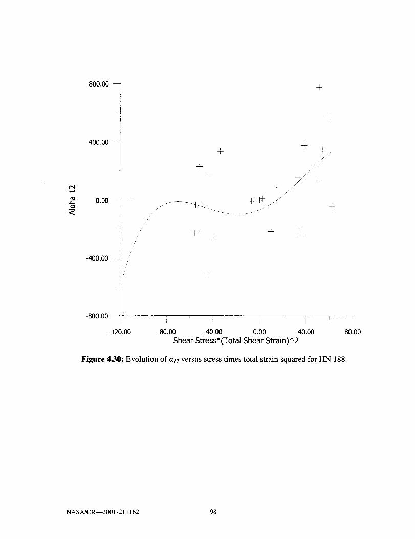
t-Q.
,,¢
800.00
400.00 --
o.oo _ 4-
//
/
/
-400.00 -- /
/
-800.O0 ÷!
-120.00
+
+
+
÷÷
/
r/
/ -H- ÷
÷
+///
+÷
q-/
/+/
+
+
÷
I iI ' ] _ I ' I-80.00 -40.00 0.00 40.00
Shear Stress*(Total Shear Strain)A2
80.00
Figure 4.30: Evolution of a12 versus stress times total strain squared for HN 188
NASA/CR--2001-211162 98

Chapter 5
Conclusions and Future Work
This chapter provides a summary of the major conclusions from both the
experimental and analysis portions of this study as well as some suggestions for future
work.
5.1 Conclusions
This study had two very distinct parts. First was the experimental portion and
the other was the data analysis portion. Both has it own set of conclusions.
Experimental
• Plastic flow in Haynes 188, 316 Stainless Steel, and lnconel 718
complicated and highly alloy dependent, with each material exhibiting
varying degrees of each of the three components of hardening; isotropic,
kinematic, and distortional.
• All subsequent yield surfaces had two distinct parts; a well defined front
side and a poorly defined backside. The front side was nearly circular in
the axial-shear stress plane and the backside was flattened.
• Subsequent yield surfaces continued to evolve through multiple cycles of
a given load path.
NASA/CR--2001-211162 99

• Even thought the three alloys tested were vastly different it appears that
the same type of evolution equations could represent the multiaxial
hardening of each material.
Data Analysis
• The Voyiadjis model adequately describes subsequent yield surfaces with
only four parameters; one isotropic, one distortional, and two backstress
parameters.
• The isotropic parameter, a, and kinematic parameters, all and a12, evolve
smoothly though the entire set of yield surface tests.
• The distortional hardening parameter, d, is difficult to describe, partly
because of the large amount of scatter in the yield points on the backside
of the yield surface.
• Evolution of the isotropic hardening parameter and kinematic hardening
parameters can be reasonably well described by simple equations.
5.2 Future Work
The work presented here attempts to quantify the evolution of subsequent yield
surfaces. This process includes many experimental and mathematically difficulties.
However, now that the groundwork is set for determining the necessary parameters for
quantifying yield surfaces there are many areas that require more attention. Of primary
concern is improving the yield surface fits. Some suggestions are,
• Reducing the amount of experimental scatter in the backside of subsequent yield
surfaces. Two approaches would apply,
1. Study the effect of probing rate on backside scatter.
NASA/CR--2001-211162 100

2. Study the effect of the offset strain target value on backside scatter.
In either case the sensitivity studies would be carried out for subsequent yield
surfaces instead of initial yield surfaces as done with the current study.
• Further investigate the increased yield surface scatter observed in IN 718 as
instead of SS 16 and HY 188.
In addition to improving the experimental data further work is needed in
developing evolution equations for the yield surface parameters. The ultimate goal is to
develop evolution equations to be used in a viscoplasticity model to predict yield surfaces
for a given plastic strain value.
NASA/CR--200I-211162 101


References
.
.
.
.
.
.
.
.
.
10.
Tresca, H. (1864) "Sur l'ecoulement des corps solides soumis 'a defortes
pression," C.R. Acad. Sci, Paris, Vol 59, pp 754.
von Mises, R. (1913) "Mechanics of Solids in the Plastically Deformable State"
NASA Technical Memorandum 88488, 1986. (translation of" Zustrand,
Nachrichten vonder Koniglichen," Gesellschaft der Wissenschaften, pp 582-592.
von Mises, R. (1928) "Mechanik der plastischen Formaenderung von Kristallen,"
Zeitschrigtfur Angewandte Mathematik und Mechanik, Vol 8, pp 161 - 185.
Prandtl, L. (1924) "Spannungsverteilung in plastischen Koerpern," Preceedings.
1 st hTternational Congress on Applied Mechanics, Delft, J Waltman, jr. Ed.,
Technische Boekhandel en Druckerij, pp 43-54.
Reuss, E. (1930) "Beruecksichtigung der elastischen Formaenderungen in der
Plastizitaetstheorie," Zeitschrift fur Angewandte Mathematik und Mechanik,
Vol 10, pp 266-274.
Ortiz, M. and Popov, E. (1983) "Distortional Hardening Rules for Metal
Plasticity," Journal of Engineering Mechanics, Vol 109 No. 4, pp 1042-1057.
Eisenberg, M.A. and Yen, C. (1984) "The Anisotropic Deformation of Yield
Surfaces," Journal of Engineering Material and Technology, Vol 106, pp 355-360.
Kurtyka, T. and Zyczkowski, M. (1985) "A Geometric Description of
Distortional Plastic Hardening of Deviatoric Materials," Archives of Mechanics,
Vol 37, pp 383-395.
Kurtyka, T. and Zyczkowski, M. "A Description of Distortional Plastic Hardening
of Anisotropic Materials," Yielding, Damage, and Failure of Anisotropic Solids,
J. P. Boehler Ed., 1990, Mechanical Engineering Publications, London, pp 97-111.
Kurtyka, T. and Zyczkowski, M. (1995) "Evolution Equations for Distortional
Plastic Hardening," International Journal of Plastici_, Vol 12, no. 2, pp 191-213.
NASA/CR--2001-211162 103

11.
12.
13.
14.
15.
16.
17.
18.
19.
20.
21.
Rees, D. W. A. (1984) "An Examination of Yield Surface Distortion and
Translation," Acta Mechanica, Vol 52, pp 15-40.
Voyiadjis, G. Z. and Foroozesh, M. (1990) "Anisotropic Distortional Yield
Model," Journal of Applied Mechanics, Vol 57, pp 537-547.
Voyiadjis, G. Z., Thiagarajan, G., and Petrakis, E. (1994) "Constitutive Modelling
for Granular Media Using an Anisotropic Distortional Yield Model," Acta
Mechanica, Vol 107, pp 1-21.
Hill, R. (1948) "A Theory of the Yielding and Plastic Flow of Anisotropic
Metals," Proc. Roy. Soc., London, Series A, Vol. 193, pp 281-297.
Arnold, S. M. and Saleeb, A. F. (1994) "On the Thermodynamic Framework
of Generalized Coupled Thermoelastic-Viscoplastic-Damage Modeling,"
blternational Journal ofPlastici_, Vol 10 No. 3, pp 263-278.
Arnold, S. M., Saleeb, A. F., Castelli, M. G. (1996) "A Fully Associative,
Nonlinear Kinematic Unified Viscoplastic Model for Titanium Bases Matrices,"
Life Predication Methodology for Titanium Matrix Composites, ASTM STP 1253,Johnson W. S., Larsen J. M., and Cox, B.N. Eds., American Society for Testing
and Materials, pp 231-256.
Arnold, S. M., Saleeb, A. F., Wilt, T. E. (1995) "A Modeling Investigation of
Thermal and Strain Induced Recovery and Nonlinear Hardening in Potential
Based Viscoplasticity," Journal of Engineering Materials and Technology,
Vol. 117, pp 157-167.
Bonder, S. R. and Partom, Y. (1975) "Constitutive Equations for Elastic-
Viscoplastic Strain-Hardening Materials," Jouranl of Applied Mechanics, Vol 42,
pp 385-389.
Bonder, S. R. and Partom, Y. (1972) "A Large Deformation Elastic-Viscoplastic
Analysis of a Thick-Walled Spherical Shell," Journal of Applied Mechanics,
Vol 39, pp 751-756.
Hecker, S. S. (1976) "Experimental Studies of Yield Phenomena in Biaxially
Loaded Metals," Constitutive Equations in Viscoplastici_: Computational and
Engineering Aspects, ASME, pp 1-33.
Michno, M. J. and Findely, W. N. (1976) "An Historical Perspective of Yield
Surface Investigations for Metals," International Journal of Non-Linear
Mechanics, Vol. 11, pp 59-82.
NASA/CR--2001-211162 104

22.
23.
24.
25.
26.
27.
28.
29.
30.
31.
32.
Phillips, A., Liu, C. S., and Justusson, J. W. (1972) "An Experimental
Investigation of Yield Surfaces at Elevated Temperature," Acta Mechanica,
Vol. 14, pp 119-146.
Phillips, A. and Tang, J. L. (1972) "The Effects of Loading Path on the Yield
Surface at Elevated Temperature," International Journal ofPlastici_., Vol. 8,
pp 463-474.
Phillips, A. and Moon, H. (1977) "An Experimental Investigation Concerning
Yield Surface and Loading Surfaces," Acta Mechanica, Vol. 27, pp 91-102.
Phillips, A. and Lu, W. (1984) "An Experimental Investigation of Yield Surface
and Loading Surfaces of Pure Aluminum with Stress-Controlled and Strain-
Controlled Paths of Loading," Journal of Engineerh_g Material and Technology,
Trans. ASME, Vol. 106, pp 349-354.
Helling, D. E., Miller, A. K., and Stout, M. G. (1986) "An Experimental
Investigation of the Yield Loci of 1100-0 Aluminum, 70:30 Brass, and an
Overaged 2024 Aluminum Alloy After Various Prestrains," Journal of
EnghTeering Material and Technology, Vol. 108, pp 313-320.
Helling, D. E., and Miller, A. K. (1987) "The Incorporation of Yield Surface
Distortion into a Unified Constitutive Model, Part 1: Equation Development,"
Acta Mechanica, Vol. 69, pp 9-23.
Helling, D. E., and Miller, A. K. (1988) "The Incorporation of Yield Surface
Distortion into a Unified Constitutive Model, Part 2: Predictive Capabilities,"
Acta Mechanica, Vol. 72, pp 39-53.
Lissenden, C. J., Lerch, B. A., Robinson, D. N. (1996) "Verification of
Experimental Techniques for Flow Surface Determination," NASA TechnicalMemorandum 107053.
Gil, C. M., Lissenden, C. J., Lerch, B. A. (1999) "Yield of Inconel 718 by Axial-
Torsional Loading at Temperatures up to 649°C, '' Journal of Testing and
Evalution, Vol. 20, no.5, pp 327-336.
Naghdi, P. M., Cailletaud, G. (1996) "Finite Element Analysis of the Mechanical
Behavior of Two-Phase Single-Crystal Superalloys," Scripta Materialia, Vol. 34,
no. 2, pp 565-571.
Taylor, G. I., Quinney, H. (1931 ) "The Plastic Distortion of Metals,"
Philosophical Transactions of the Royal Society, London, Vol. A230, pp 323-363.
NASA/CR--2001-211162 105

33.
34.
35.
36.
37.
38.
39.
40.
41.
42.
Wu, H. C., Yeh, W. C., ( 1991 ) "On the Experimental Determination of Yield
Surfaces and Some Results of Annealed 304 Stainless Steel," hTternational
Journal ofPlastici_, Vol. 7, pp 803-826.
Ellis, J. R., Robinson, D. N., and Pugh C. E. (1985) "Time Dependence in Biaxial
Yield of Type 316 Stainless Steel at Room Temperature," Journal of Engineering
Materials and Technology, Vol. 105, pp 250-256.
Lui, K.C. (1977) "Yield Surfaces and Elastic-Plastic Behavior of Type 304
Stainless Steel," ORNL/TM-5421, Oak Ridge National Laboratory, Oak Ridge,
TN, April.
Hecker, S. S. (1971) "'Yield Surfaces in Prestrained Aluminum and Copper,"
Metall. Trans., Vol. 2, pp 2077-2086.
Khan, A. and Wang, X. (1993) "An Experimental Study on Subsequent Yield
Surfaces After Finite Shear Prestraining," International Journal of Plasticic_,
Vol. 9, pp 889-905.
Williams, J. F. and Svensson, N. L. (1970) "Effect of Prestrain on the Yield Locus
of 1100-F Aluminum," Journal of Strain Analysis, Vol. 5, pp 128-139.
Kalluri, S. and Bonacuse, P. J. (1990) "A Data Acquisition and Control Program
for Axial-Torsional Fatigue Testing," Applications of Automation Technology to
Fatigue and Fracture Testing, ASTM STP 1092, A. A. Braun, N. E. Ashbaugh,
and F. M. Smith, Eds., American Society for Testing and Materials, Philadelphia,
pp. 269-287.
Ellis, J. R. and Bartolotta, P. A. (1997) "Adjustable Work Coil Fixture Facilitation
the Use of Induction Heating in Mechanical Testing," Multiaxial Fatigue and
Deformation Testing Techniques, ASTM STP 1280, S. Kalluri and P. J. Bonacuse,
Eds., American Society for Testing and Materials, pp 43-62.
Lissenden, C. J., Lerch, B. A., Ellis, J. R., and Robinson, D. N. (1997)
"Experimental Determination of Yield and Flow Surfaces Under Axial-Torsional
Loading," Multiaxial Fatigue and Deformation Testing Techniques, ASTM STP
1280, S. Kalluri and P. J. Bonacuse, Eds., American Society for Testing and
Materials, pp 92-112.
Hecker, S. S. (1976) "Experimental Studies of Yield Phenomena in Biaxial
Loaded Metals," Constitutive Equations in Viscoplasticity: Computational and
Engineering Aspects, ASME, pp 1-33.
NASA/CR--2001-211162 106

43.
4.
45.
46.
47.
48.
49.
50.
51.
52.
53.
54.
Lissenden, C. J., Walker, M. A., and Lerch, B. A. (2000) "' Axial-Torsional Load
Effects of Haynes 188 at 650°C, '' Multiaxial Fatigue and Deformation: Testing
and Predicition, ASTM STP 1387, S. Kalluri and P. J. Bonacuse, Eds., American
Society for Testing and Materials, pp 99-125.
Gil, C. M., Lissenden, C. J., and Lerch B. A. (1998) "Determination of Yield in
Inconel 718 for Axial-Torsional Loading at Temperatures up to 649°C, '' NASATechnical Memorandum 208658.
Kiemele, M. J., Schmidt, S. R., and Berdine, R. J. (1997) Basic Statistics: Tools
for Continuous Improvement. Air Academy Press, Colorado Springs, Colorado.
Gil, C. M. (1998) "Determination of Yield and Flow Surfaces for Inconel 718
Under Axial-Torsional Loading Temperatures up to 649°C. '' Thesis, Penn State
University.
Hirth, J. P. and Cohen, M. (1970) "'On the Strength-Differential Phenomenon in
Hardened Steel," Metallurgical Transactions, Vol. l, pp 3-8.
Ziebs, J., Meersmann, J., Kuhn H. J., and Ledworuski, S. (996) "'Experimental
Techniques for Testing Materials Under Multiaxial Loading," Multiaxial Fatigue
and Design, A. Pineau, G. Cailletaud, and T. C. Lindley Eds., Mechanical
Engineering Publications, London, pp 173-193.
Winstone, M. R. (1983) "Influence of Prestress on the Yield Surface of the Cast
Nickel Superalloy MAR-M002 at Elevated Temperature," Mechanical Behaviour
of Materials/V, J, Carlsson and N. G. Ohlson Eds., Vol. 1, pp 199-205.
Lubliner, J. (1990) Plasticity Theory. Macmillan Publishing Company, New
York.
Kassner, M. E., Ziaai-Moayyed, A. A., and Miller, A. K. (1985) "Some Trends
in the Elevated Temperature Kinematic and Isotropic Hardening of Type 304
Stainless Steel," Metallurgical Transactions, Vol 16A, pp 1069-1076.
Klarstrom, D. L. (1993) "Wrought Cobalt-Base Superalloys," Journal of
Materials Engineering Performance, Vol. 2, pp 523-529.
Wegener, K. and Schlegel, M. (1996) "Suitability of Yield Functions for the
Approximation of Subsequent Yield Surfaces," International Journal of
Plastici_, Vol. 12, no. 9, pp 1151-1177.
Wu, H. C. and Yeh, W. C. (1987) "Some Considerations in the Endochronic
Description of Anisotripic Hardening," Acta Mechanica, Vol. 69, pp 59-76.
NASA/CR--2001-211162 107

55.
56.
57.
58.
59.
Gupta, N. K. and Meyers, A. (1994) "An Alternative Formulation for
Interpolation Experimental Yield Surfaces," hlternational Journal of Plasticit3,,
Vol. 10, no. 7, pp 795-805.
Gil, C. M., Lissenden, C. J., and Lerch, B. A. (1999) "Unusual Nonlinear
Response of Some Metallic Materials," Mechanics of Materials, Vol. 31,
pp 565-577.
Gil, C. M., Lissenden, C. J., and Lerch, B. A. (1998) "Investigation of Anomalous
Behavior in Metallic-Based Materials Under Compressive Loading," NASATechnical Memorandum 206640.
Cho, H. W. and Dafalias, Y. F. (1996)"Distortional and Orientational Hardening
at Large Viscoplastic Deformations," International Journal ofPlasticicty, Vol.
12, no. 7, pp 903-925.
Yen, C. F. and Eisenburg, M. A. (1987) "The Role of a Loading Surface in
Viscoplasticity Theory." Acta Mechanica, Vol 69, pp 77-96.
NASA/CR--2001-211162 108

Appendix A
Catalog of Yield Surface Data
Appendix A begins with a list of all specimens tested and the dimensions of each.
The second section contains all yields surfaces collected along with the fit data for each.
A.1 Specimen Dimensions
Material SpecimenNumber
Haynes 188 HYII 82
HYII 85
316 Stainless
Inconel 718
HYII 86
HYII 89
HYII 90
610-01
610-04
610-05
Test
Path
III
I
II
I
III
Table A.I:
I
II
Ill
11 IV
14 VI
16 I
23 II
27 III
28 V
Outside Inside
Diameter(in) Diameter(in)
1.0241 0.8669
1.0227 0.8660
1.0238 0.8656
1.0231 0.8663
1.0237 0.8653
1.0257 0.8675
1.0252 0.8678
1.0257 0.8680
0.8225 0.6244
0.8220 0.6238
0.8195 0.6245
0.8230 0.6244
0.8190 0.6236
0.8203 0.6242
Specimen dimensions and test matrix.
NASA/CR--200I-211162 109

A.2 Yield Surface Data
All yield surface data are presented here. Figures A. 1 through A. 12 show HN
188 data, Figures A. 13 through A.27 show SS 316 data, and Figures A.28 through A.32
show IN 718 data. The experimental data is represented by plus signs and diamonds
(the first and second repeated surfaces), the fits are shown by a solid line, and the initial
surface is shown by a dashed line. In addition, the model parameters a and d as well as
the R 2 values are shown on each graph.
NASA/CR--2001-211162 110

-!t
oo2_
] L ! i [
Point A
a = 0 8077
d=O0
R_2 = 02575
+o b+
i .
I F
Axial Slress IM Pa_
[
]i
F
I _ I , I
Poinl C
a = 0 6428
d = -6 26e-5
R_2 = 02600
©
, © + _r
I r I
Axial %tre_s ¢_1Pa_
I
4oo._
I L I L
400._
Poinl E
-_t_.oo _a = 0.4306
d = -8 66e-5
I R^2 = 0305
4,oo_
C'
\+
O
0
I F
ooc 4CODOAxial Slress J,l Pa_
I I , I , I
0 .+
_/ L
:" + 4-
: i
_, o_
• /
Point G
a = 02601
d = -4.1e-5
R'2 = 0250
I [
Axial Stres_ _M Pa_
[
4OO.OO
I , I _ I
Point I
a = 0.2202
d : -I 4800e-4
R^2 = 0 18_1
,:)_ O
+//f
'+ o _+!
\_q_-_..__.#.. j'O
©
-,_ oo ooo 4000o
_,xial SI[¢SS _M Pa_
Figure A.h Haynes 188, Path I, Points A-I, Cycle 1, HYII-89.
NASA/CR--2OOI-211162 1 1 1
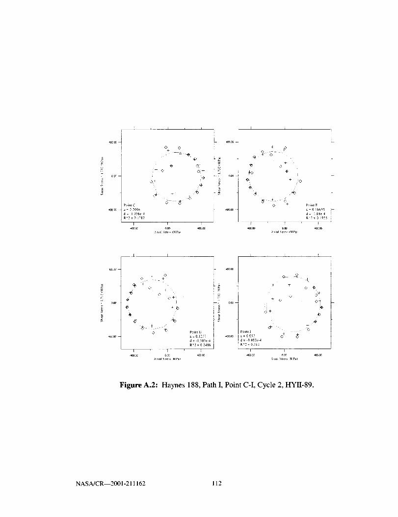
i
40000-
l+ O
4÷
O O+
4>
e_+
FII
-t
÷ +o
4-
O
+ /©
y_
= D 2006 a = 016635
= -1356e-4 d = -I.08e-4
R^2 = 01782 R^2 = 0 1055
[ r F I _ ! !
_ooDoAU_I _tress _MPa,°°° 400._ _00 Axial Slless _M Pa_°°G
4000(3
[ , t I [ L _ i r
I ÷ O
<2 ....... +
Q-. + > ".+ ,
,t, o+ i
© Poinl G
a=01237
d = -1303¢-4
R_2 = 0.2486
Poinl I
-- _oooo -_ a = 0057
i d = -3 802e-4
R^2 =0.161
I 1 [ I I [
-,100 (_A_lal Stte_s _M Pat°0(J '_C_._ -40000 Axial S_r'_s^_IM Pa_
,_¢) Oo
÷ 5-o @
0 O+
i
,,ff
O- -, __ _ _>÷
o+
Figure A.2: Haynes 188, Path L Point C-I, Cycle 2, HYH-89.
NASA/CR--2001-211162 112

_ Point A43_3 o¢ a = 1 044
d=00
R^2 = 0.278
I
_00
F L t , I
O'+
I
o.o_ 400oo
_xial Seres_ 4MPa)
. 000
[ t I i
Poinl B
a = 07377
d = -13e-4
R^2 = 02:I8
<_+ 4?
o'+
[ I I
AxlM Slress0,IPa)
i Poim C
_,'c¢ 00 a = 0.6643
d = -3.37e-4
R_2 = 0222
I
-400 0¢ 000 ,_o00
_, xial Slress qMPII
000-
Poinl D
-_oo m -_ a=07186d = -5.84e-5
I R_2 = 0301
4OOOO
I L [ I
q_ ..... ,.+
I I
0.00 4oo.0o
A xial Stress _I_ Pat
I L I , I
Point E
a = 0.6281
d = -2 a}e-4
R_2 = 0 228
I r
-_oo 00 oO0 4(1ooo
Axial Stress _H Pa_
Figure A.3: Haynes 188, Path 11, Points A-E, Cycle 1, HYII-86.
NASAJCR--2001-211162 113

[ i i I
Poinl F
a = 0596
d = -46 le-4
R^2=0217
<2
I
.accoo ooo
_xlal Mres_ EMPa_
-L
rOooo
OCC-- ¸
I
-_00CC -_
I , I
Point G
a=0477
d = -5 4"e-4
R_2 = 0217
+
0 +
÷ +
0 ,C,
<:W- A_
I I
oo ooc'ixial Stress 4M Pa,
i
4000C
[ i
Point H
a = 06281
d = -2.43e-4
i:
_' _ _+
+
E 1 I
_OD.O0 ooo 4c_oG_xial Stress 0,1Pa_
Figure A.4: Haynes 188, Path II, Points F-H, Cycle 1, HYII-86.
(The data for point I was bad therefore not fit was performed.)
NASA/CR--2001-211162 114

I I I
Point B
a=0351
d= -271e-4
R_2 = 01Q6
L-
[ _ [
_oo oc, ooo 4oGooAxial Sires* IM Pa}
, t , [
Point C
a = 035-*
d = -3,15c-4
Ra2 = 0202
o _+ ÷o
© : + //
\ +
4C_00 000 _ O0
_X_ial Stress IM Pa_
, J k LI
Point D
] a = 00.417
.*oo c_ d= -I 51e-2
R'2 = 0142
+
O O
+,_" © O "-+
o*, 4-o
[
Point E
a = 0464
d = -4,19e-4
R^2 = (l,0q
J I L I
'0" .... q_z+
+
+] OOC, 4:
0 O, i
• , +Q
©4--, '-_
I F I I I I
-,_,oooo oo0 aoooo _oooo o oo .1oo0o
_xial Stress tMPa_ A _.tal Stress 0,1Pa_
Figure A.5: Haynes 188, Path 1I, Points B-E, Cycle 2, HYII-86.
NASA/CR--2001-211162 115

t
Point F
a=0.189
d = -3.25e-4
R^2 = 014_
+O + ".4-
_+ ,v iO +:
b-,_,$.,5 *v
1 I l
._oo ooo _ o_A_iai Stress 4M Pa_
L
4O0¸00
L
Point G
a = 0-_55
d = -2 .t6¢-4
R_2 = 0.275
+©
+ ...... .
¢%__ +" ¢,
+0 o
C,_ + -r©
I I
Axial Stress O,t Pa_
] J I
4c_9n
_+
o._
I
/+© ©_ t++ +0
+ i ! _
l L I , L
_G¢ 4
+ +"O
i
Point I
Point H _onoo a = 0255
_ooc_ a=0225 d = -4 79e-4
d = -4 4t_e-4 R^2 = 0178
R'2 = 017_
I I I t 1
-_O000 0_ 40000 _O3.00 000 _000A xial Stre_s d_l Pa_ A xlzl Stress _M Pa_
Figure A.6: Haynes 188, Path II, Points F-I, Cycle 2, HYII-86.
NASA/CR--2001-211162 116

-tiJ
t , I , I
_- +
/% O _ +
i Point Bci = -4 I 7e-4
R"2 = 0.198
I
-4Oo oo
I [
ooo ,_oc_4 xi_l s Ires_ (M Pa)
t L L L i
•_00OG
I J L
Point D
a = 01845
d = -3 4e-4
R_2 = 01357
© O0 G
_oo.oo
Point E
a = 06281
d = -2 43e-4
R'2 = 0.228
O +
+
+ " © 0 +_ ._/
© ©
+ 0 +iO
! _ r I F f
Axial Stress O.IPa_ Axial Stress !MPal
Figure A.7: Haynes 188, Path II, Points B-E, Cycle 3, HYII-86.
NASA/CR--2001-211162 117

Point F
R_2 = 0.206
ooG--
I
++OD0o --
4oooo
!_
..... ', LF4- © _ G ooG
I
+:'C, +o , L
t
PoJI_I 0 I
;+= 004.1ql
d=-16¢+_
R'2 = 0,%1"
+
4-
4,
+ ÷
00 ÷
©
+++.++.++]
I
t
Axial Strrss IMPI+
"_+_ 9- + +-.+,+• . ,G"
i + ©
++ + o+++© q- +'©
ooo i
9 <> + ++-
:+- +._',9 • ++4+ 4- •
i Poial l{
_ a=O 1385
d = -7 5¢-4
_0,146
,sO0 03o_ 4<x'koo
A_ial Stress _MPa_
¢2
7
aO_OC
ooo.
. <> '_
4-
©
© : O+ ............ q-"
PoJrll 1
= 0628 I
tl = .2 43¢-4
R_2 = O 22_J
%
2
++
xlal _lr_ss _MPa_
Figure A.8: Haynes 188, Path 1I, Points F-I, Cycle 3, HYIJ-86.
NASA/CR--2001-211162 118

i
Point AJ, a = 1 086
,moo0 _ d = O0
R_2 = 0310
J
t
oo(1 !
r
-4oo o0
, I , I
ooo 400o0
Axill Stress {M Pal
I , [ , t
P_dnl B
a = 07768
d = -:; 90e-4
R_2 = 0,253
I
.aoo.o0
_.C, ,6'
,_+ ,e
r i
o.c_ ,_,oooo
Axial Stress i MPal
, I , I
*b' O O_
Point C
a = 04822
d = -3 63e-1
R_2 = 0t22
40000 oo0Axial Stre_s _MPa_
F_
J
Point Da = 0_152
,,,oo.m d = -I.16e-4
R'2=0125
I
4000_ -
I r
4O0¸00 .40600
J J , t
©
...... 4,,-.. +
/ " . ...
4-
o <_i
o,,+
I
0O0
,axial Stress (M Pa}
I
i I I I
o ,¢,.__.."_ . o
%
£ +,
_- + /
.._ ..... +
E I
i Poinl F
Poinl E a = 02058
a=03105 -_o3 oo d=7%-4
d = -3.61e-3 R_2 = 0180R_3=0t13
....'*"-£'- ¢' e.," +o \_-
/
+
e _
\ • .,4:
+
I ! r [ I ! L
.,ic_ o0 oo0 400._ -4_300 _00 40600Axlal Slre_s d'4 Pa_ Axial $tress IM Pa_
iFigure A.9: Haynes 188, Path m, Points A-F, Cycle 1, HYII-90.
NASA/CR--2001-211162 119

L i k i I
o( + ._
"_.-.=_. -7-- 'G7 C,
Point B
,_=OI21q
d = -4 55e-4
RZ2 = 0 I40
[ r I
ooo 4oo_
_,ual Str,es_ qMP_)
Ei
© + :'
, ]
,_, ÷'I
L _v 0 Point C
a= 0.1146
d = -6 27e-4
R_2 = 0.0#5
409O6 ooo
I
I _ J t
P_>int D
a = 02280
d = -9.45e-3
R_2 = 0120
©
++
.3 .... +/- _\ ,.%
+ / 0 _"
¢, o÷i
© +_
_ <>+._,- e'<_
-£.
o.O6-
]
o(3o _oooo
Axial St[es_ !M Fa_
J , I , I
©
+. -'4"-_
C>O"" 4-
_÷ <> +
+
"-4.+
Point E ]a : 00980 v-d = -4 87e-3
R^2 = {3085 ]
-,Oo oo oooAxial SIleSs ,M P|I
I
Point F
a = -0.076
d = -I 162e-3
R_2 = 0.073
: I t
O6 (3oo _._
Axial Stress (MPa)
Figure A.10: Haynes 188, Path HI, Points B-F, Cycle 2, HYII-90.
NASA/CR--2001-211162 120

ooo
_.oo oo
i I , Ii k
Poinl A
a = 00620
d=00
R_2 = 0421
-_,oo oe ooo 4o000Axial 51reds 4M Pa_
.7-
-4000:
J _ t
Point B
a = 07558
d = -I 25e-3
R_2 = 0221
©
+0 @
©+ :-I,_
I i I
-4OO0O ooo 4(io_
Axial Stress _,1 Pa_
I , t I
Q-- "_- 4>
_- _+ <., .+
6-
.... ¢S- _'
Poinl c
a = 04158
d = -t 60e-_
R'2 = 0 200
I ! I
_oooo 00: ,Ic_ooA x ial Stress +M PI
I
Poinl Da = (12746
4oooo , d = -I 0qe-3
i R'2=010Ir
, I , I
'C,
O
<> + ÷
Z.+ + <_
I r [
o.00 aooooA xial S Ires'. r M Pat
I , J , i
<_/+ <_ "X
_ ©+
_ _:i, !
,_,!, :+ 0
v'--':_ _0 Point E
a = 0 1785
d = -2.66e-3
R'2 = 007'_
i _ t L [
/
+/'O
/
O_ \,
_oooo
ooo
Point F
a = 0.081
d = -4 00e-4
R_2=0L54
I
-_oo oo
_,
+
1 I I I I
Axial Stress _MPa_ .Axial Stre_s _M Pa_
Figure A.11: Haynes 188, Path lIl, Points A-F, Cycle 1, HYII-82.
NAS A/CR--2001-211162 121

I , I _ i
i
0_
t Poinl B
a = 0053
qot; oa d = -5 38e-4
R"2 =0 137
+-.)
+
Z
F I 1
ooo 4oooo
:_ _lat sl_e_ 4M PaJ
@ +©
400_
©
Poinl (-
a = _1028_
d=q I_e-4
R'2 = 0087
-4OOOO oooA_lal Stre_s qM Pa)
I
40OO0
J
I
Point D
a = -0 0382
d = -0 g6e-4
R_2 = 0040
C,©
+
+
+ i
_+iO -C'/
÷
!
ooo ,_3oo
._,xtal SlleSs 4MPa_
L
t L I , J
i -"+ .... <
©+
4o
+
_F +
-Q, - .©
Point E
a = 00810
d = -374e 3
R _2 = 005v
A xlal Stress _M Pa_
]
i , I 1
Point F
a = .010q
d = -1 37e-3
R_2 = 0.075
© a-
©+ "O.+
i
+_
+
+ ,'
.Q,_ -
I I I
A xlal Slress _M Pa_
Figure A.12: Haynes 188, Path 111,Points B-F, Cycle 2, HYI]-82.
NASA/CR--2001-211162 122

-200DO !
J _ [ L l
Point k
a = 0.835Q
d = fl(!
R_2 = 0.375
<>+ -_
, [
-20000
r [ _ I '
0 O0 200 DOAxial Stre_ IMPa_
4oooo J I _ I , I k l
-2OODO
Point C
a = 0.482
d = t?.6e.4
R^2 = 0.218
40000
-400 O0
[ ' I _ I
20000 0.00 20000Axial Stress (M Pa)
40000 ]
200¸00
Point E
a = 0.2086
d = -1,03e-3
R^2 = (I,I42
4000o i I I
Point B
a = 07042
d = -_,4'.)e-4
R_2 = (L201
20(?0:3 --
40000
AO000
[ L ! I
ooo
I
20000 |
400.00 ]
[i ' [ ' I _ I
-200 DO ODO 200 D0 40000
kxial Stres_ IMPI)
L I J I I I
Poinl D
a = (/.3321
d = -6.01 e-4
R_2 = 0.151
4_ 4,
0
[ I ' I
40000 -40000 20000 000 20000
_xial Stress (MPal
f I I I
d* +
Figure A.13:
-4DO00 -200 00 000 200.DO
Axial Stress (MPa_
40000
316 Stainless Steel, Path I, Points A-E, Cycle 1,610-01.
NASA/CR--2001-211162 123

4oooc _ _ r _ (
Point Fa = 0.105 =
d = -3,65e-3
i R'2 = 0175J
20000
20000
[-40000 I
4OO00
-aa+ + +
, i
' { _ I ' I
-200 oo ooo 2ooocxial Stresa (M Pa_
IL-
L
, iqO0O0
I _ L , I _
. ©
Point (i
a = 0.3328
d=-6 16c-3R_2=011H
2_ OC 0 _ 2_A_ial Stress (M Pa
4oo_ i _ L
i Point H
a = 0.032) d = -t.60e-3
i R_2 = 0151
oo(2 t
1
[I
20000 1
4oo00! _ 1400.DO 200O0
L I t E
÷. -o +_© \
@
o.oo 200.00 400.0(2A_ial Stress ibt Pa_
Point I
a = 0.0425
i d = -l.6be-I
I i R_:=o.1_:
20000
7 ooo ,.__ "_
1/
-41_ O0
400(i,0 200C_) 000 20000Axial Sirens fMPa)
Figure A.14:316 Stainless Steel, Path I, Points F-l, Cycle 1,610-01.
NASA/CR--2001-211162 124

4OOCO
20000 --t
400.00
-40000
I i ! t t J
Point B
a = O.Oq4
d = --1.49¢-3
R_2 = 0.121
r200.00
+
4-
000
Axial StressiMPal
*0ov % F"<3" % ---
_>
--+-_ 5
I ' I '20000 400 O0
200.00
-40O(;0
4O0O0
t , I L t , 1
PLaint C
a = 0.093
d = -2.96e-3
R_2 = 0.100
+ ,,9. © '_-
+ k @
I-200.00 0OO 20000
Axial Slress IMPa!
40000
2OOCO
-200OO
400¸OO
-400 DO
L , I _ I ,
Point D
a = 0.0004
d = -2.00e-3
R_2 : 0115
4> • /: +>
....÷
400 OO
200OO -
OOO
J I , L , I _
Point E
a = 0.1101
d = -2.7e-3
R_2 = 0,176
-;.<@- __<_.+
{ +'<_
4"-÷.... _>+4>
=(_
l [ I -4oo.oo _ I [ , [ r
-200 OO 0OO 20000 4OOOO -40000 -200 (_ 0OO 200.00Axial Slress IMPal Axial Stres_ (.M Pa)
Figure A.15:316 Stainless Steel, Path I, Points B-E, Cycle 2, 610-01.
i
40000
F
400¸00
NAS A/CR--2001-211162 125

I i I i I i
Poinl F
a = -0.026
d = -1.4e-2
R^2 = 0.I46
i i i I _ Ii
7,
Point G
a = -0.0.36
d = -1,4e-2
R"2 = 0.[03
©<b
+
_+ C' ,© 4- 4)4C_- 4, 4-
;'_ + _ ¢,'+ 4-4,
_' +> %,__4- '0
4¢eoo F r [ , E _ I _ I !
40000 2t_ 0.00 20000 40000 -200.00 0 _ 20_ 00
Axial Stress IM Pat Axial Slr¢_s IM Pa)
!
20000 i
40000
-400 O_
40000 i ' I , J _ I L
-20e O0
r Point H[
q a =-0AI4d = -l,00e-_
R_2 = 0.634
Point 1
a = -0.100
d = -2.00e-3
R_2 = 0.105
4,= ..... _.
O (+
+
4, ;9_.--_
I4oooo -4OO£_' ' r I I ' I [ I
-4OOOO -2OOOO OOD 2O000 400.1_ 200.OD o oo 2OO00A xial Stress (M Pal A xial S Ire ss i M Pa
Figure A.16:316 Stainless Steel, Path I, Points F-I, Cycle 2, 610-01.
l
7
ao_oo
NASA/CR--2001-211162 126
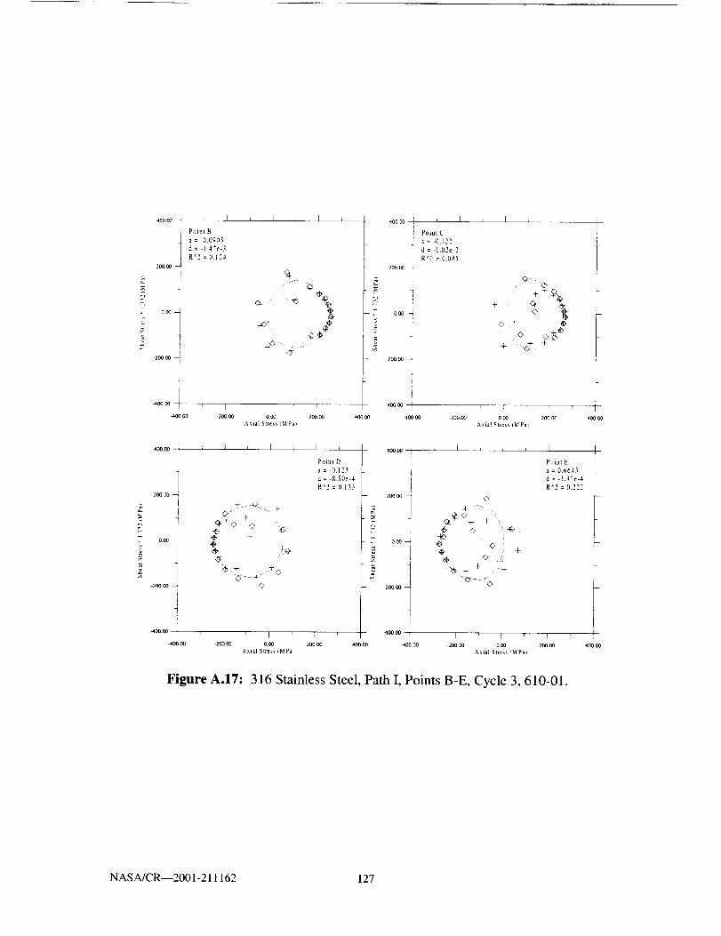
-200 O0 l
40C O0
_OOO0
B , t , 1
Point B
a = -0.0905
d = -1,47e-3
R_2 = 0,124
÷o, ......
I J t , J
Point C
a = -0,122
d = -I.02e-2
R^2 = 0.085
-- 200_ --
. OOS
i'200¸0(I[ i I i I r / 40000 ' r ' I I
-200CO 000 20000 40000 40000 -200OO 0 CK) 20000
Axial Stress ):M Pa_ Axial Stress I_,l Pal
G, t _,
C:_ _
20000
i L400OO
[ I I I
Point D
a= -0.123 i
d = -8.50e-4
R:2 = 0.133
r
L I , i
©± -.+ .+....---,
<>" + _+ +_+,9 ©4> <> _ o '@
_.+ :_<_ _ + + . +
20000 --
J
ooo
-20000 i
-40000
Point E
a = 0.6643
d = -3.37e--I
R^2 = 0.222
400.00 -2oo o_ o.oo 200 oo 400 oo -20o.00 ooo 20000
Axial Stress (MPa) Axial Slress eM Pal
Figure A.17:316 Stainless Steel, Path I, Points B-E, Cycle 3,610-01.
r40000
4OO¸00
NASA/CR--2001-211162 127

o.0o-
J , I J t i
,--2- "--.
g + ° i+ Q
4OOOO t
i
o_
-200 (10 !
4OOOO
4OOOO
[
-20_ O0
Point H
a = -0A85
d = -4.31c-3
R_2 : 0.050
Point F
a = -0A :_1
d = -2.6qe-3
R_2 = 0.136
' 1 I
0oo 20000 400.00
A_ial Stress (MPa_
L J J t _ --
+. -- --÷
_ oo %
+
+ . + .¢©o,
20000
r_
0.00
-200 00
q_ --P-+
c4-
o+
I ' ) ' i
400.00 20000
4oooo I ' II
] Poinl 1
d a = -0A3()d = -3,77t'-3
R^2 = 0.078
200.00 --
,E
2_
• o0o_
_- -20000
l 4oo co
4O0 O0
000 200 O0
:k xial Stress _MPa_
-- 4-4,
O ;' ©
O+ g
Point G
a = -0150
d = -8.05e-3
R^2 = I).0t,3
400¸00
F
-200.00 000 200,00 400.00 200,00 0 O0 200 0() 400 (K)
Axial Stress (MPa) Axial Stress (MPal
Figure A.18:316 Stainless Steel, Path I, Points F-I, Cycle 3, 610-01.
NASA/CR--2001-211162 128

L
=
40000 I I [
Poinl A
a = 1143
d=0,0
R_2 = 0516
20000
000 ]
20000
40000 r I I ' I
-40000 -2000(_ 000 200O0
Axial StressqM Pa)
i
400 130 1 I
Point B
2oo130_ R_2 =0223
I
' - "4°°°0 I
40000 40000 -200
I r
0DO 20000
A xial Stress i },1Pa
40000
200.00 --
0¸130
20000
40000
400_
t , ] L i
<>i+ _->
Point C
a = 0.8603
d = -5.02e-4
R_2 = 0.236
J ' I-2DO 130 0130
,Axial Stress qMPa)
20000 --
ii20000 -
[ r 40000
20000 40000 -40000
I _ I , I
Point D
a = 06438
d = 4.35e-3
R_2 = tL153
+<>
I ' I ' [ '20000 000 20000
Axial Stress (.M Pa _
40000 I
0.130
2130130
-400 O0
-4000O
t , I , I ,
Point E
a = 0.5083
d = -6 28e-3
R_2 =O.tll
+_
I ' I ' I20000 000 200 130
Axial Stress (MPa_
Figure A.19:316 Stainless Steel, Path 11, Points A-E, Cycle 1,610-04.
40000
NAS A/CR--2001-211162 129

4_ 00 i
i]
i
2OO O0 4
000
] i i i
Poinl F
a = 0.4182
d = -6 24e-3
R^2 = 0122
_oo00 i I ' I
40000(1 -200.00 0 CO 200 00
Axial Stress Uq Pa_
i 40000
]
I 200_00
. 000_
-200 00
-40O.00
Point G
a = 03328
d = -6.17e-3
R^2 = 0.163
, I , I
I T I ' I
20000 000 200.00
Axial Stress tM Pap
40000
PoiBl tta = 0,1880
d = -2.84e-3
| R^2 =0.155
20000
+b
40000
200¸00
000
-20000
i
Poinl 1
a = 0.20(_
d = -3.15e-3
R^2 = 0.t25
I i I i
O
_oo 00 i I I _ _t00 00 ' I I I
_O000 20000 0.00 200.00 40000 -40000 -200 CO 000 20000
_xial Slress IMPal Axial Slress (MPal
Figure A.20:316 Stainless Steel, Path II, Points F-I, Cycle 1,610-04.
40000
NASA/CR--2001-211162 130

_0000 L I t I J I I
r
o_
20000_ PointB
a : 0.1310
d = -2.76e-3
R^2 = 0.131
-490 00 i, [
-,IO3 0:3 -200 00
, I , ! _ I
O+ _ _' ++ : 7"
40000 !
200¸00 1
0_00 i
1 i F000 200 oc, ,_oo 00(3
A x ial S Ire ss _M Pa i
-20000
Point C
a = t).lT-l:_
d = -2.Sqe-_
R_2 : (LI 20
"40000 -200 00 000 20(I 00 400 00
Axial _lress (MPa_
400.00 1
20000
0¸130 t
H
-200_00 1
_C,O,00 I
t, , I , I J
Point D
a = 0,1210
d = -2 45e-3
R^2 = 0.110
40000 k I
Point E
= 0.0844
d = -3.1 le-3
! R^2=0.10_
2_NI
<>_ _--"<> ?-' o-+-*-_-,,+ 0 + , 000 ,÷ ,,
•2oo00 @_t"_.__ _
] I I -400.o0 , ] r
-200 00 000 20000 -40000 200_ 0.00 200.00
Axial Stress (MPa_ Axial Stress IM Pal
40000
, J J i , i
Figure A.21:316 Stainless Steel, Path H, Points B-E, Cycle 2, 610-04.
40O 00
NASA/CR--2001-211162 131

200.00
OCO
20000
400¸00
400¸00
, i
Point F
a = i).058 _
d = -2.71e-Z
R'3 = O.07q
' I200 CO
i I J I i
%. 2,J
ooo 1
200 00
I
t 400 co rI
i
[
2coco
t _
40000
Point G
a = 0.0i51
d = -3.31e-3
R'2 = 0.102
, I _ I ,
_o °° *
_+ -_
' t I ' -400 co i ' I ]
i
O_ 20000 40000 20000 Oco
_xial Stress _M Pa_ _.xla] Stres_ ¢MPa_
I
P
t
20OOO 4OOOO
400.00 J
2OOO0
°t-21XIO0
Point H
A a = 0.0087
! d = -2.75e-3
i R_2 = 0.1"6
-4oo0o t [
_0000 -200 CO
I , I , ! , I I t ,
_00®- ,a,*'*_%.
. % ?/ _ %* _ I-- o00- + -÷od_.. + Q.- _ '_-- + Q
200.00
Point I
a = 0.0037
d = -2.ile-3
R_2 = 0.185
_100 00! i I I i
O.CO 200.00 400 00 4CO 00 -2CO co 0.00 20000
Axial S,ess _M Pal Axial Stress IMPa!
I4OO.co
Figure A.22:316 Stainless Steel, Path II, Points F-I, Cycle 2, 610-04.
NASA/CR--2001-211162 132

I i F _ .
<>+ ,i'
20000
000--
-200CO --
Point B
a : -0.046
d = -2,80e-3
R '2 : 0.075
2+00.00 i ! r [ I '
400_ -2_ O_ 2OOOO 4000A xlalStress (M Pa
400.00
4ooo0 t _ 4 , ] J [
, t i I , I
_+ _
i
Poinl C
a : -0.042
d = -2.20e-3
R^2 = 0.1 20
I i )
400 O0 -20000 O_ 20000 40000
Ax}al Slress _bl Pa_
Poinl D
a : -0,067
d : -I .19e-3
R_2 : 0.100
I _ t , I I
[20000 _ 20000 --
-i* 0.00 000
+
+' © <)
-200.00 <k'+- _7
<_ _ _a_> _ -200.00
i 400 00 I
/
_+¢+
7,t.O © ._'
" +-_ 7" +
Point E
a = -0.115
d : -2.06e-3
R_2 = 0.083
' I I
E_'00 1 I ' r I I
40000 -20000 000 20000 '400.00 -400.00 -20000 000 20000 40000
Axial Stress (MPal A_ial Stress (MPa_
Figure A.23:316 Stainless Steel, Path II, Points B-E, Cycle 3,610-04.
NASA/CR--2001-211162 133

4OOOO
2(;0 O0
20000 j
4OOOO !
40000
J
Point F
a = -0,0640
d = -2,00e-3
R^2 = 0A 20
i [ i I
':a- -+ --4= -
© {>4-,¸
-}-
o o +<>+¢
L
I
4oooo t [
[_oint G
I a = -0.064
i d = -2,73e-3
R:2 = 0.118
200 oo
20000 0OO 20000
Axlat Stress {M Pa)
20000
..... . -. Q
*. _ +
O +% +O
,O+- + O
¢,+ _,ej%,a<:. _
14OOOO' I I ] _ I ' ! I
400.00 -40000 200 OO OOO 20000
Axial Stress _,| Pa i
.oooo-_--_
200OO !
OOO I
-2_OO I PoitllH
a = -0A630
d = -2.44¢-3
R^2 = 0.080
.40o00
+'__'*-_%__-©
\
+ %
<) /
40000
200OO
OOO
•_ +.,t-
+_-
_c+, * +
4: - +-" +
-- -200 OO
Point I
a = -0.120
d = -2.60e-3
i R^2 = 0.103]
I l _ _ ' 1 4o000 / i _ I
400.oo -2OO OO 0.00 20000 40000 400.00 -200 O0 0 OO 200,00
Axla_ Slfess lM Pab Axial Stress {M Pal
Figure A.24:316 Stainless Steel, Path If,Points F-I, Cycle 3, 610-04.
40000
NASAJCR--2001-211162 134

4o_.oo i I
2OO00 i
000
|
-2O0O0 _ Poinl A
a = 0 9t)18
d=0,0
R:2 = 0.42 I
-40000 20000
, I J 1
L
I'
, I400_000 20000
Axial Stress IMPal
2000(]
_0000 i
Point B
a = 0.7812
d = -5 .I 7e-4
R_2 = 0217
: }
F I ]
20000 o o0 20000
Axial Stress tMPa_400 OO
LOO0
20000 i
L I J i k I L
Point C
' a = 0.2841
d = -4 13e-2
R^2 = 0.163
@ +',
; <>
J I F
200.00 0.O0 20000
Axial Slress FMPa!
i
Point D
a = -0.0027
20000 -- d = -I .7]e-d
R_2 = 0.103
, J , I
©
, _ 'Ok; +
': .¢: @
I
2OO00
' I ' ]
o0o 20000Axial Stress IMPa_
400.00
2000(1
40000
400.O0
J I , I k I I
@
¢, ._
O
+
Point E
a : -0.0841
d = -2.53e-3
R_2 : 0.007
I I I J [ ,
K20000 40000
[_ 400O0 i20000 --
r
0_O0
200_O0
Point F
a : -0.1720
d = -1.OOe-t
R'2 : 0.141
-400.O0 _ [
4OO0O -200 O0
/
O: +_
+0
_'\
r r r ' I 1
-2OO.O0 0.O0 00(1 20000
Axial Stress OdPat _xial Stress (MPat
Figure A.25:316 Stainless Steel, Path m, Points A-F, Cycle 1,610-O5.
NASA/CR--2OO 1-21 1162 135

40000 i i .
200_
000
20000
t Point B
, a= -0,174n
d = -I ,25e-3
R"2 = 0105
400 t_ r I
_400 O0 200CO
L I b I
%
+
r
[ E ] i
D00 200.00
_. xial Stress (MPaw
40000
40000
20000 --
-200O0
J I , 1 J ]
+
Point C
a = 41.267
d = -2.32e-3
R_2 = 0.0Q3
I i 1 I
20000 0 00 20000Axial Stress IM Pal
I400.00
_0000! , I
Point D
a = -0A64
d = -5.%#e-2
R'2 = 0.134
200120
00(3
20000 !
40000 i , I
40000 20OOO
I t :
© ©
+ + +_-_
+ <> © .ex¢_'-......÷...._,-r
f ' IO O0 200 OO
A _.ial Stress EMPa_
i
4OO¸0O
4OO¸OO t L [
4
I
200,00 I - +"_o <>.
_, +
2 ' .c <>
J40000 1 _ I
40000 20000
, I L t J
©
+
] i
000
_ial Stress tM Pa_
Point E
a = -0,230
d = -7,01¢-3
R_2 = 0087
I
2O0O2 4000O
40000 J '
200,00
+ <>- '°+4_@a,@
©
+ ©_ + :
+
o00
.200.00 _ Point F
a = -0,15qd = -I.10e-2
R'2 = O.184
-40000 _ I
-40100 -200.00
+
@
I r 'OOD 200.00
Axial Stress IMPI!
Figure A.26:316 Stainless Steel, Path Ill, Points B-F, Cycle 2, 610-05.
NASA/CR--2001-211162 136

4OK)O0
2OO O0
OCO
200 O0 --
_OOCO
400_
2_.00
t I _ ] 4oooo J L ] I , i , I
+
Point B
a = 0.6643
d = -3,_7e-4
R'2 = 0.222
[ ' [ ' r
200.00 0 DO 20000
,XKialSt[cs_ IMPa_
C
20000 -_ /. 0
-. +
i -6 _ ,
©
-2oooo <_ ©
-40000 r ] i
Point C
a = -0.214
d = -_.08e-3
R_2 = 0.053
I i ] r
-2oo 13o o o0 20000
Anial Stress _MPa!
I , t , I
Point D
a = -0.0027
d = -1 73e-4
R'2 = 0.103
: q-
[
-200O0
' I ' 1
OO(3 200OO
A_ial Stress IMPa)
] i I4000(3i
20000 t
g
2ooo_
Point F
a = -0,246
d = -I .41e-3
R_2 = 0.0.35
AO000 -2_
40000 !
, I c r J I
200
+
-20000
40000 I
\
Point E
a : -0.3360
d : -2.21e-3
R_2 = 0073
1 _ [ r [
-40000 -20(I 0_
I , J ,
000 200 PA)
A xial S Ire ss 4M Pa
+ _t
+ +
©\* + ._
©
' r ! ' !
o.13o 20000 400 oo
A xial St[ess /M Pa_
Figure A.27:316 Stainless Steel, Path HI, Points B-F, Cycle 3, 610-05.
NASA/CR--2001-211162 137

T
I00000
50000 --
ODO
-500O0 I
tO00 O0
I_,00
t , i _ 1
Point A
: 1.12
d = 0.()
R_2 = 028R
+ '_-
+, +
':I-,. • .4/%"+ _g
I ' r r I F500_ 0_ 500
A xiaI S tI¢_ _M Pal
100000
r L i J I , J
Point C
a = 0.?0q0
d = -1.33e-4
R'2 = 0.222
+
-t- /÷
_L
I ' [ i 1 '5O0OO O_ 50000
xial Stres_dM Pad
50000
•500_00 t
.1Don_oo
÷
H ¸ + , +
÷
.+. + +
] I I I
Point E
a = 0.b660
d = -6 61e-3
R^2 = 0.183
i000O0
5{3000-
• 000--
-5_00
-ICK)OO0
I i [ i
-500 OO OC_A xial Stress _1,1Pa
I
5O000 1000.00
L ; I _ I ,
+
+
+
+
+ •
Poinl G
a = 0.533]
d = -" 02e-3
R_2 = 006"
ooo-
-500.DO
I000.00
I i ! _ ]
Point [
a = 0.269
d = -1.28e-3
R_2 = 0.110
/
/
i
4-
+'
+
+ +
4
+:+
_*._..'
/_r
tO00 CO 50000 0.00 500.00A',IM Sirens IMPal
10OOOO
Figure A.28: Inconel 718, Path I, Points A-I, Cycle 1, IN-16.
NASA/CR--2001-211162 138

50000
-50000
-lO_
50000 --
, I
Poinl C
a = 0.3:;68
d = -I 56e-3
R_2 = 0.168
h i L I _ t 1ooooo
-J3.. "--.-b " "
__ +++
+ - .+ .-- ---+/
' I ' r r I '4OO O0 0.00 50000
A'dal Stress IMPa)
4 J _ I
5OOCO
• OOO
-500 O0 ]
-IOOO 00I
1000 OO -looO OO
J I i I , t
+
+_/
/
+ + i!:+ + +
+ : i+
+ ++ t
@\ '
Point E
a = 0.227
d = -n.5_5
R_2 = 0.013
[ 1 I '5OOOO ofio 5OOOO
_.",ial Stre_s tMPa_
[ -4-
+ ++' +!
+: i
+, + t-:'
+ -+ .....
1.ooo oo [ r I I I I j
-I(XX).OO -5OO.OO O.OO 5OO,OO
Axial Stress IMPa!
Point (5
a = 0,267
d = -0285
R_2 = ¢0.01()
?:. OOO
4 5oooo!
1000 OO I l
t Point i
a = 0.2511
d : -3.01c-4
R'2 = 0.185
500130
+
+ +':I +!
!+ +
, + +
.tL"+ -. .
100000 -IOOOO0 -SOO.00 O.OO 50000
A x ial S tress I bl Pa IIOOOOO
Figure A.29: Inconel 718, Path I, Points C-I, Cycle 2, IN-16.
NASA/CR--2001-211162 139

lOO0.O0
50000
5¢XJO0 -
I
tO00 O0
.1000.00
i L i [ , i
+A-
+
+
+
[
50O O0
Point A
a = 08914
d:00
R_2 = 0.361
[ [
00'3 50000
AXial S([e_ iM P3)
7
i(<)4).00[ k ] .
50000
i+
+\
50000
-100000
-1000_00
• 4-_- "+4-
4.
4-
+
+
+\
4.
Point C
a = 04390
d = -1.59e-3
R_2 = 015_
' I I i ! ,
-5c4).oo o.oo 500 O0
Axial Stress tM Pa}
tO00 OO i
soooo
tCt_ O0
, J
Poinl E
a = 0.42"
d = -1 be-3
R_2 = 0.068
+
+/: _',
i + +,
+ + __,"
I J [ 100000
P
-- $oooo _
L
++_ + _:
++
+ •
4.
Point 1
a = 06643
d = -3.37e-,.1
R_2 = 0.222
' l [ I -zooooo ] _ I I _ I-$00.00 000 5000D 1000.00 1000 O0 -500.CO 000 50000
Axial Stress IMPa_ Axial Stress IMPa_
Figure A.30: Inconel 718, Path 11, Points A-I, Cycle 1, IN-23.
1000 O0
Ii
[
m
tO00£_
NASA/CR--2001-211162 140

I000 O0 i i t i
_ + +
, ...... ,. --
5001_+
:÷ +
5ooo_ -I Poinl C
Ia = 0.2404
d = -3.60e-3
R"2 = 0.051
tooo (_{ ' I
.iooooo -5OOOO O,O0 5OO
A ximlSlress (M Pa_IDO0.O0
I _ I , I
I I! a = O2Oa
I d = -2 30c--_
R'2=004_
++
ooo < + ".4//
i + 4-
14- + ,'
soo _ ,, + +
• + +
1ooooc .sooco ooo 5OOO0Axial 5Ires_ _MPa,
O_
, I , I
Point E
a = 0.30_
d = -1.50e-3
R_2 = O.ll4
i'+ L
4-::
-_ 4_
+, +
4-'_-
ql _-%_
{ ' i ' {
500_ ooo 50000
4 xial _)tre_s (M Pal
L
• __ =k ___ .
+ :_,
ooo + +,.
c- + -F
5OOOO
Poinl I
a = 0 t02
R '2 = OOTI
iooooo .soo oc ooo sooooAxia] Stress(MPm,
t
L
lOOO o_
Figure A.31: Inconel 718, Path If, Points A-I, Cycle 2, IN-23.
NASA/CR--2001-211162 141

i00_C_ I
i
500¸00 _
, I , L L I I
+
+
+ #+
Point A
a = 0..1032
d=0.O
R_2 = 0.187
lo00 oo I I !
1_oo .500 txl ooo 500 DoAxial Stress tM Pa_
1000.00500C_ J I___
_2
J
t--
o.oo
50O0O
Poim B
a = 0,138
d = -2 22e-3
R_2 = 0.075
-1coo oo I
-100000 5oo.oo
, t , I ,
_ -4.
+<+
+
+
+
+ 4÷J
-4-
+
I' I I ' 1
0 00 50000 tO00 O0
Axial Stress IM Pa!
_00oo_+s,+-+''',
o00', 4- _
50000
-1coo I_
, I J t L I 100o00 ;
Point C
a = 0.2336
d = -0.990
R_2 = 0.002
5-I
-1ooo,00
!-500.00 0.00 500.00 1_,00 -1000.00
Axial Stress iMPa_
-50000
J [ , I J i ,
! Point D
a = 0.0qSOq
d = -1.45e-3
I R^2 = 0.021
"4- ..._ --q-
A-
-500,00 000 50000
Axial Stress IblPat
!1
1000 O0
Figure A.32: Inconel 718, Path m, Points A-D, Cycle 1.
NASA/CR--2001-211162 142

100000 150000
I]
0 O0 --
SO000 --
-iooooo
-100000
0.00
I
50000
10o000
-iooooo
I , i , t
+
÷--++
+
,m+ +
+
Point A
a = 0.909
d=O.O
R^2 = 0,t 14
i k
l I I '50000 000 500 DO
Axial Stress _MPa}
IC410O0 i i
_000 -
000--
-500O0
Point C
a = O, 1732
] d = -4,1c-3
i R_2=0,127
100000 [
-lOC_ oo .50000
I , I
4-.......÷--- +4.
4: ++
4.
r I ' J 'ooo SHOO
Axial Stress 4MPal
I , I , I i
-4-
'i:4- +t
+ /
Point D
a=0.1239
d = -2 07e-3
R'_2 = 0101
lO00oo
_ 50000_2
_- 7" 0,00
L=
-5110 OD 1
iooooo
t , I , ] ,
d---..
I i l ' [ ' ' [ ' i,500.00 000 SO000 100000 -1000O0 -500 00 0OD
Axial Stress _MPal Axial Stress IMPa)
Point E
a= 0.186
d = -8 49e-3
R^2 = 0.68
]50000 IDOOO0
Figure A.33: Inconel 718, Path IV, Points A-E, Cycle 1.
NASA/CR--2001-211162 143


Appendix B
Yield Surface Fit Data
Cycle Point _ (MPa) _ (m/m) a d o_11 o_12
1 A 0 0 0.8077 0 0 0
1 C 314 0.015 0.6428 -6.30E-05 49 -8
1 E -348 -0.0013 0.4289 -1.60E-04 -94 -10
1 G -422 -0.015 0.2691 -4.10E-05 -120 -8
1 I 406 0.0013 0.2308 -8.90E-05 73 -14
2 C 424 0.015 0.202 -9.04E-05i 101 -7
2 E -445 -0.0013 0.1663-1.00E-04 -131 -5
2 G -489 -0.015 0.1238 -9.80E-05 -176 -11
2 I 458 0.0012 0.058 -3.21E-04 90 -10
Table B.I: Haynes 188, Path I, HYII-89.
NASA/CR--2001-211162 145

Cycle Point x (MPa) y (m/m) a d o_11 o_12
1 A 0 0 1.044 0 -20 -5
1 B 169.8 5.41E-03 0.737 -1.30E-04 0 33
1 C 186 1.09E-02 0.664 -3.37E-04 -2 38
1 D -175 5.42E-03 0.719 -5.85E-04 -5 -43
1 E -185 -7.65E-04 0.628 -2.43E-04 -4 -49
1 F -205 -5.45E-03 0.596 -4.36E-04 -10 -53
1 G -217 -1.09E-02 0.477 -5.48E-04 -10 -45
1 H 190.6 -5.47E-03 0.429 -3.68E-04 -5 34
1 I 220.8 i 6.91E-04
2 B 215 5.41E-03 0.351 -2.71E-04 -10 49
2 C 231 1.09E-02 0.354 -3.15E-04 -10 59
2 D -206 5.42E-03 0.417 -1.51E-02 -10 -52
2 E -218 -7.51E-04 0.464 -4.19E-04 -10 -55
2 F -229 -5.24E-03 0.189 -3.25E-04 -10 -40
2 G -258 -1.09E-02 0.555 -2.36E-04 -10 -99
2 H 210 -5.47E-03 0.225 -4.49E-04 10 35
2 I 246 -7.05E-04 0.255 -4.79E-04 -10 62
3 B 255 5.40E-03 0.223 -4.17E-04 -15 54
3 C 256 1.19E-02 0.1556 -4.80E-04 -10 51
3 D -230 6.35E-03 0.1845 -3.40E-04 10 -34
3 E -254 7.00E-06 0.4737 -4.80E-04 1 -110
3 F -268 -4.50E-03
3 G -279 -9.96E-03 0.4391 -1.60E-03 0 -117
3 H 219 -4.55E-03 0.1385 -7.50E-04 0 10
3 I 267 1.88E-03 0.1318 -6.30E-04 -10 51
Table B.2: Haynes 188, Path II, HYII-86.
NASA/CR--2001-211162 146

Cycle Point _ (MPa) e (m/m) • (MPa) 7 (m/m) a d ix11 ct12
1 A 0 0 0 0 1.086 0 0 0
1 B 225 0.0106 105 0.0077 0.7768 -3.90E-04 25.5 14.7
1 C -364 -0.0106 37 0.0077 0.4822 -3.63E-03 -78 2
1 D 305 0.0106 -174 -0.0076 0.3152 -1.16E-04 57.5 -56
1 E -454 -0.0106 -32 -0.0076 0.3105 -3.60E-03 -123 -7
1 F 322 0.0008 202 0.0006
2 B 358 0.0106 196 0.0077 0.1219 -4.55E-04 56 48
2 C -507 -0.0106 35 0.0077 0.1146 -6.27E-04 -170 0
2 D 389 0.0106 -240 -0.0076 0.228 -9.46E-05 112 -115
2 E -572 -0.0106 -40 -0.0076 0.098 -4.87E-03 -210 -20
2 F 376 0.0008 254 0.0006 -0.076 -1.16E-03 70 75
Table B.3: Haynes 188, Path HI (First Run), HYII-90.
Cycle Point c (MPa) e (m/m) _ (MPa) _, (m/m) a d o_11 0_12
1 A 0 0 0 0 0.962 0 -10 0
B 227 0.0106 106 0.0077 0.7558 -1.25E-03 22 12
C
D
-367
314
-446
-0.0106
0.0106
-0.0106
21
-168
-23
0.0077
-0.0076
-0.0076
0.4358
0.2746
0.1785
-1.06E-03
-1.09E-03
-2.66E-03
-72
62
-111
-59
-10
F 320 0.0008 209 0.0006 0.081 -4.00E-04 86 73
B 384i 0.0106 208 0.0077 0.053 -5.38E-04 97 77
2 C -546 -0.0106 33; 0.0077 0.0283 -1.15E-03 -168 10
2 D 416 0.0106 -246 -0.0076 -0.038 -9.86E-04 100 -110
0.081
-0.109_
-0.0106-589
383
-3.74E-03
-1.37E-03
-0.0076
0.00060.0008
-228
84
-45
270
-60
87
Table B.4: Haynes 188, Path HI (Second Run), HYII-82.
NASA/CR--2001-211162 147

Cycle Point _ (MPa) _ (m/m) a d o_11 _z12
1 A 0 0 0.8359 0 -4 0
1 B 130 0.0075 0.7042 -3.49E-04 22 0
1 C 150 0.015 0.482 -9.60E-04 29 1
1 D -175 0.0075 0.3321 -6.01E-04 -48 -6
1 E -195 -0.0006 0.2986 -1.03E-03 -58 0
G
C
D
G
H
C
D
G
H
-209
-221
206
216
231
244
-232
-257
-270
-269
245
269
275
283
-260
-294
-298
-308
266
296
-0.0075
-0.015
-O.O075
0.0006
0.0075
0.015
0.0075
-0.0006
-0.0075
-0.015
-0.0075
0.0006
0.0075
0.015
0.0075
-0.0006
-0.0075
-0.015
-O.OO75
0.0006
0.1957
0.083
0.032
0.0425
0.094
0.093
0.004
0.1101
-0.0026
-0.036
-0.114
-0.1
-0.0905
-0.122
-0.123
-0.141
-0.131
-0.15
-0.185
-0.13
-3.65E-03
!-1.40E-03
-1.60E-03
-1.66E-03
-1.49E-03
-2.96E-03
-2.00E-03
-2.70E-03
-1.69E-03
-1.40E-02
-1.00E-03
-2.00E-03
-1.47E-03
-1.02E-02
-8.50E-04
-2.37E-03
-2.69E-03
-8.05E°03
-4.31E-03
-3.77E-03
-64
-62
40
65
71
90
-100
-120
-118
-120
40
95
100
102
-83
-106
-120
-125
64
114
-4
-8
-8
-2
-2
-1
-4
-11
-11
-4
-4
-2
-2
-3
Table B.5:316 Stainless Steel, Path I, 610-01.
NASA/CR--2001-211162 148

Cycle Point _ (MPa) I ¥ (m/m) a d o_11 cd 2
1 A 0 I 0 1.143 0 0 0
1 B 70 5.40E-03 0.971 -3.28E-03i 1 11
1 C 75 1.08E-02 0.8603 -5.02E-03 0 17
1 D -77 5.40E-03 0.6438 -5.35E-03 -7 -15
1 E -87 -4.00E-03 0.5983 -6.82E-03 -1 -23
1 F -96 -5.40E-03 0.4182 -6.24E-03 0 -26
1 G -100 -1.081=-02 0.3328 -6.161=-03 -3 -28
1 H 98 -5.801=-03 0.188 -2.84E-03 5 14
1 I 101 3.00E-04 0.206 -3.15E-03 5 26
2 B 110 5.40E-03 0.131 -2.76E-03 0 28
2 C 120 1.08E-02 0.1743 -2.59E-03 0 34
2 D -117 5.401=-03 0.121 -2.45E-03 -2 -31
2 E -124 -4.001=-03 0.844 -3.11E-03 0 -35
2 F -126 -5.401=-03 0.0587 -2.71E-03 0 -45
2 G -135 -1.08E-02 0.151 -3.31E-03 0 -46
2 H 129 -5.80E-03 0.0087 -2.75E-03 0 30
2 I 131 3.00E-04 0.0037 -2.11E-03 -1 43
3 B 138 5.40E-03 -0.046 -2.80E-03 2 47
3 C 150 1.08E-02 -0,042 -2.20E-03 0 51
3 D -140 5.40E-03 -0.067 -1.19E-03 -10 -42
3 E -150 -4.00E-03 -0,115 -2.06E-03 -10 -39
3 F -157 -5,40E-03, -0,064 -2.90E-03i -7 -57
3 G -161 -1.08E-02i -0.064 -2.73E-03 -7 -62
3 H 149 -5.80E-03 -0.163 -2.44E-03 -14 32
3 I 164 3.00E-04 -0.126 -2.69E-03 -12 53
Table B.6:316 Stainless Steel, Path II, 610-04.
NASA/CR--2001-211162 149
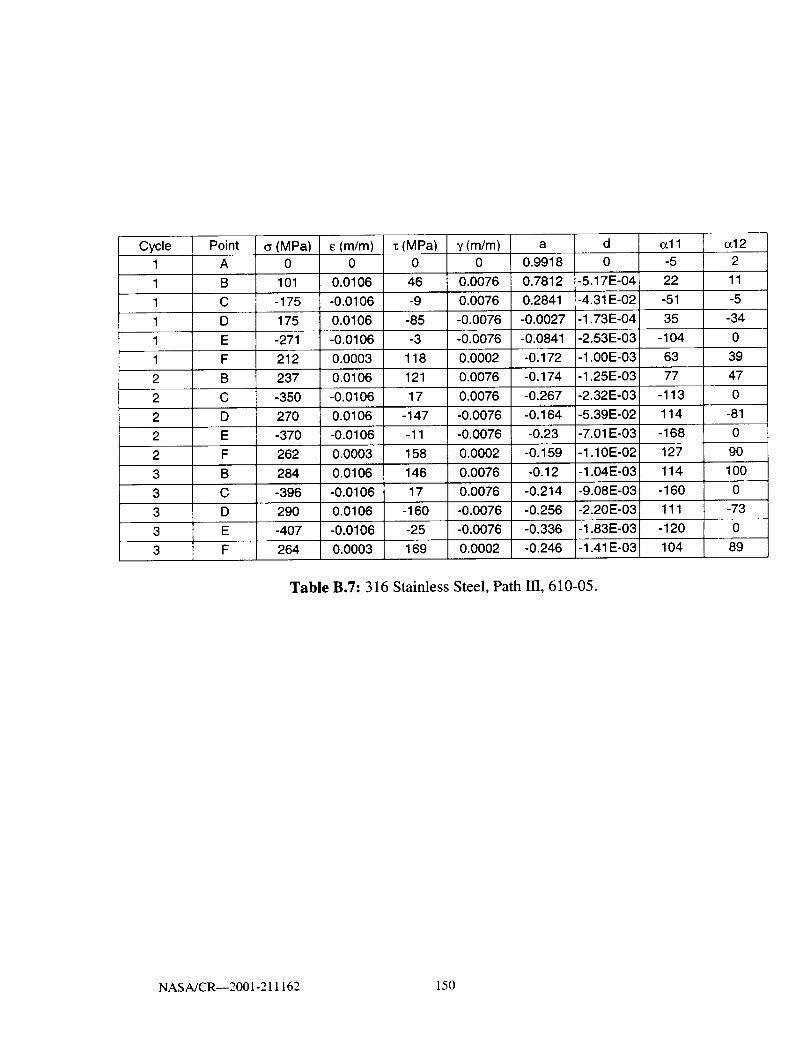
Cycle Point _ (MPa) _ (m/m) T (MPa) 3' (m/m) a d (zl 1 c_12
1 A 0 0 0 0 0.9918 0 -5 2
1 B 101 0.0106 46 0.0076 0.7812 -5.17E-04 22 11
1 C -175 -0.0106 -9 0.0076 0.2841 -4.31E-02 -51 -5
1 D 175 0.0106 -85 -0.0076 -0.0027 -1.73E-04 35 -34
1 E -271 -0.0106 -3 -0.0076 -0.0841 -2.53E-03 -104 0
1 F 212 0.0003 118 0.0002 -0.172 -1.00E-03 63 39
2 B 237 0.0106 121 0.0076 -0.174 -1.25E-03 77 47
2 C -350 -0.0106 17 0.0076 -0.267 -2.32E-03 -113 0
2 D 270 0.0106 -147 -0.0076 -0.164 -5.39E-02 114 -81
2
2
3
E
F
B
C
D
E
-370
262
284
-396
290
-407
264
-0.0106
0.0003
0.0106
-0.0106
0.0106
-0.0106
0.0003
-11
158
146
17
-160
-25
169
-0.0076
0.00O2
0.0076
0.0076
-0.0076
-0.0076
0.0002
-0.23
-0.159
-0.12
-0.214
-0.256
-0.336
-0.246
-7.01 E-03
-1.10E-02
-1.04E-03
-9.08E-03
-2.20E-03
-1.83E-03
-1.41 E-03
-168
127
114
-160
111
-120
104
9O
100
-73
89
Table B.7:316 Stainless Steel, Path 111, 610-05.
NASA/CR--2001-211162 150

Cycle Point
A
C
E
G
C
E
G
(MPa)
796
-795
-871
760
833
-8OO
-880
756
(m/m)
0.015
-0.0002
-0.015
0.002
0.015
-0.0002
-0.015
0.002
1.12
0.709
0.666
0.533
0.269
0.3368
0.152
0.176
0.25
-1.33E-04
-6.60E-03
-7.00E-03
-1.28E-03
-1.56E-03
-2.70E-01
-1.56E-01
-3.12E-04
all
-146
221
-255
-380
110
144
-350
-376
135
o_12
25
-25
15
Table B.8: Inconel 718, Path I, IN-16.
Cycle Point
A
(MPa) y (m/m)
0.8914
o_11
-145
oc12
1 C 535 1.06E-02 0.4399 -1.59E-03 -145 160
1 E -470 -1.70E-03 0.427 -1.60E-03 -145 -100
1 G -529 -1.06E-02
-5.55E-03
-3.60E-03
1.70E-03474 -145
-145
0.369 110
1402 C 535 1.06E-02 0.2494
2 E -455 -1.70E-03 0.303 -1.59E-03 -145 -63
2 G -527 -1.06E-02 0.249 -2.30E-03 -145 -110
2 I 466 1.70E-03 0.302 -3.08E-03 -145 80
Table B.9: Inconel 718, Path II, IN-23.
NASA/CR--2001-211162 151

Cycle Point _(MPa) _(m/m) _(MPa) _(m/m) a d _11 _12
1 A 0 0 0 0 0.4032 0 -160 0
1 B 760 0.0106 385 0.0077 0.138 -2.22E-03 144 85
1 C -1050 -0.0106 127 0.0077 0.2326 -0.99 -418 80
1 D 736 0.0106 -470 -0.0077 0.0959 -1.45E-03 -165 -180
Table B.10: Inconel 718, Path HI, IN-27.
Cycle Point
1 A
1 C
1 D
1 E
(MPa) £(m/m) T (MPa) y(m/m)
0.999
o_11
-160
0O2
740 0.02 245 0.015 0.1732 -4.19E-03 100 38
-585 0.0058 -400 0 0.1239 -2.07E-03 -160 -129
-857 -0.002 -128 0 0.186 !-8.49E-03 -260 10
Table B.11: Inconel 718, Path IV, IN-I 1.
NASA/CR--2001-2I 1162 152


REPORT DOCUMENTATION PAGE FormApprovedOMB No. 0704-0188
Public reporting burden for this collection of information is estimated to average 1 hour per response, including the time for reviewing instructions, searching existing data sources,
gathering and maintaining the data needed, and completing and reviewing the collection of information. Send comments regarding this burden estimate or any other aspect of this
coltection of information, including suggestions for reducing this burden, to Washington Headquarters Services, Directorate for tnformation Operations and Reports, 1215 Jefferson
Davis Highway, Suite 1204, Arfington, VA 22202-4302, and 1o the Office of Management and Budget, Paperwork Reduction Project (0704-0188), Washington, DC 20503.
1. AGENCY USE ONLY (Leave blank) 2. REPORT DATE 3. REPORT TYPE AND DATES COVERED
October 2001 Final Contractor Report
4. TITLE AND SUBTITLE
Behavior of Three Metallic Alloys Under Combined Axial-Shear Stress at 650 °C
6. AUTHOR(S)
Jason E Colaiuta
7. PERFORMING ORGANIZATION NAME(S) AND ADDRESS(ES)
Pennsyh, ania State University
University Park. Pennsylvania 16802-1009
9. SPONSORING/MONITORING AGENCY NAME(S) AND ADDRESS(ES)
National Aeronautics and Space Administration
Washington, DC 20546-0001
5. FUNDING NUMBERS
WU-708-3 f- 13--00
NCC3-597
8. PERFORMING ORGANIZATIONREPORT NUMBER
E-13020
10. SPONSORING/MONITORINGAGENCY REPORT NUMBER
NASA CR--2001-211162
11. SUPPLEMENTARY NOTES
This report was submitted as a dissertation in partial fulfillment of the requirements for the degree of Master of Science
to the Pennsylvania State University, University Park, Pennsylvania, August 2001. Project Manager, Bradley Lerch,
Structures and Acoustics Division, NASA Glenn Research Center, organization code 5920, 216--433-5522.
12a, DISTRIBUTION/AVAILABILITY STATEMENT 12b. DISTRIBUTION CODE
Unclassified - Unlimited
Subject Categories: 26 and 39 Distribution: Nonstandard
Available electronically at hl_;//_ltrs._c.nasa._ov/GLTRS
This publication is available from the NASA Center for AeroSpace Information, 301-621-0390.
13. ABSTRACT (Maximum 200 words)
Three materials, Inconel 718, Haynes 188, and 316 stainless steel, were tested under an axial-torsional stress state at
650 °C. The objective of this study was to quantify the evolution of the material while in the viscoplastic domain. Initial
and subsequent yield surfaces were experimentally determined to quantify hardening. Subsequent yield surfaces (yield
surfaces taken after a preload) had a well-defined front side, in the prestrain direction, but a poorly defined back side,
opposite the prestrain direction. Subsequent yield surfaces exhibited isotropic hardening by expansion of the yield
surface, kinematic hardening by translation of the yield surface, and distortional hardening by flattening of the yield
surface in the direction opposite to the last prestrain. An existing yield function capable of representing isotropic, kine-
matic, and distortional hardening was used to fit each yield surface. Four variables are used to describe each surface.
These variables evolve as the material state changes and have been regressed to the yield surface data.
14. SUBJECT TERMS
Inconel 718; Haynes 188; Stainless steel; Yield surfaces;
Multiaxial stress; Inelasticity; Viscoplasticity; Strength differential
17. SECURITY CLASSIFICATIONOF REPORT
Unclassified
NSN 7540-01-280-5500
18. SECURITY CLASSIFICATIONOF THIS PAGE
Unclassified
19. SECURITY CLASSIFICATION
OF ABSTRACT
Unclassified
15. NUMBER OF PAGES161
16. PRICE CODE
20. LIMITATION OF ABSTRACT
Standard Form 298 (Rev. 2-89)Prescribed by ANSI Std. Z39-1B
298-102

