beer game order policy optimization using genetic algorithms · beer game order policy optimization...

Liuc Papers n. 179, Serie Metodi quantitativi 17, suppl. a ottobre 2005

1

BEER GAME ORDER POLICY OPTIMIZATION USING GENETIC ALGORITHMS Jordi Bosch Pagans, Fernanda Strozzi, José-Manuel Zaldívar Comenges∗

Contents

1. Introduction

2. The Beer Game

2.1. The simulation model

2.2. The ordering policy

2.3. The fitness function

3. Genetic algorithms

4. Beer game parameters estimation with GA

5. Results

6. Conclusions

References

1. Introduction

The Beer Distribution Game (“Beer Game”), developed at the Sloan School of Management

in early 1960’s (Jarmain, 1963), is a classic supply chain problem widely used in graduate

business programs to teach the concepts of supply chain management (Mosekilde et al., 1991).

The goal of the participant in the game is to minimise the costs of maintaining sufficient

inventories of beer while at the same time avoiding out-of-stock condition that could lead to loss

of customers. The Beer Game is notable for its ability to confuse typical human players

(Sterman, 1988, 1989) giving rise to instabilities in the supply chain as well as demand

distortion (Chen et al., 2000). The game is also used to illustrate how different decision policies

influence the dynamics of a distribution system.

∗ European Commission, Joint Research Centre, Institute for Environment and Sustainability, T 272, 21020-Ispra

(VA), Italy

Liuc Papers n. 179, suppl. a ottobre 2005

2

Sterman (1989) formulated a four parameter discrete model for the order policy, based on the

theory of bounded rationality (Davis et al., 1986; Einhorn & Hogarth, 1985) and showed that

this model captures the main aspects of the decisions taken in the game by real players.

Mosekilde and Larsen (1988) were first to show that a time-continuous version of the Beer

Game model could produce deterministic chaos and other forms of complex behaviour

(Zhanybay et al., 2003).

In this work we are going to analyse the optimal order policies, i.e. the optimal parameters of

the Sterman model, when a step-change occurs in the customer demand. The optimal policy

considered is the policy that gives the minimum cost, accounting both for the costs to maintain a

stock of goods and for the costs of having a backlog when it is not possible to satisfy the

demand. Two scenarios have been analysed: all sectors apply the same order policies, or

different policies are applied from sector to sector. The search of the optimal solution has been

performed using Genetic Algorithms (Holland, 1975) due to the complexity of the objective

cost function, which has many local minima and, in the case of different policies, many

parameters.

The application of GAs optimisation techniques is a novelty in the case of Beer Game model

but they have been applied in several managerial problems such as portfolio optimisation and

job scheduling (Yen-Zen Wang, 2003).

Better performances are obtained when sectors apply different order policies compared with

the same order policy. This is not surprising since when the participant applies different order

policies there are eight parameters to optimise compared with two parameters when the same

order policies are applied. Furthermore, when participants apply the same order policy, the

optimal policy found using GAs is different from the analytical values obtained by Mosekilde et

al. (1991). The differences will be discussed in the paper.

2. The Beer Game

The Beer Game is a realisation of a production-distribution system on four levels: Factory,

Distributor, Wholesaler and Retailer, see fig. 1. The orders starting from the customer go to the

Retailer, then to the Wholesaler, the Distributor, and finally reach the Factory. In the mean time,

previous orders are moving from the Factory down through the supply chain until they reach the

customer. This is a typical game for students that have to manage their stocks in order to cope

with the variation of the customer demand, and at the same time trying to avoid out-of-stock

conditions. The game is widely used in management schools as a means to convey to students

the causal relationships between their decision-making and the behaviour of supply chains. The

J. Bosch Pagans, F. Strozzi, J.-M. Zaldívar Comenges, Beer game order policy optimization using genetic …

3

typical results of the game are counterintuitive, because large oscillations appear in the order

rate based on small increase in the customer demand (Sterman, 1988).

Figure 1. Basic structure of production-distribution system with state variables and orders flow (left arrow) and goods flow (right arrow) in the Beer game model.

In order to simplify this production-distribution system, several rules were defined (Jarmain,

1963):

• there is only one inventory at each level initialised with 12 cases of beer;

• the time delay from passing of orders and shipments from one stage to the next is fixed

to one week (one time period of the game);

• the production time is taken to be three weeks, and it is assumed that the production

capacity of the brewery can be adjusted without limits;

• each week customers order beer from the retailer, who supplies the requested quantity

out of his inventory.

A further typical simplification is that customer demand is four cases of beer per week until

week 4 and steps to eight cases of beer per week at week five. In this paper we have analysed a

set of customer demands that changes, at week five, from four l to fifteen cases and then we

have forced the system with a higher demand, i.e. forty cases, to test if the limit values found

are maintained.

The objective for the participants (stock managers) in the game is to minimise cumulative

sector costs at the end of the game. Considering the costs associated with inventory holding

(€0.50 per case per week), stocks should be kept as small as possible. On the other hand, failure

to deliver on request may force customers to seek alternative suppliers. For this reason, there are

also costs associated with having backlogs of unfilled orders (€2.00 per case per week).

Stock managers, in all the sectors, have to decide, at the beginning of each week, the amount

of beer to be ordered from the immediate supplier.


4

2.1 The Simulation Model

The simulation model consists of a high-dimensional iterated map that provides the sequence

of operations that each sector should perform. The boxes in Fig 1 represent the state variables.

Each variable has an initial letter that indicates the respective sector; thus R stands for retailer,

W for wholesaler, D for distributor and F for factory. For example, in the wholesale sector,

WINV is the inventory of beer, WBL the backlog of orders, WIS and WOS represent incoming

and out going shipments, respectively, where WIO is the incoming orders, WED is the expected

demand and WO

the orders placed by the wholesaler. One time step later, WO

becomes incoming orders to the distributor, DIO. The same notation is employed in the other

sectors with the exception of the factory where there is a production rate, FPR, instead of placed

orders and FPD1 and FPD2 represent the production delays. The exogenous customer order rate

is given by COR.

The difference equations of the model (Thomsen et al., 1992) that represent the operations

conducted in each sector may be written for the wholesaler sector as example:

⎩⎨⎧ +≥+−−+

= −−−−−−−−

otherwise 0 if 11111111 tttttttt

t

WIOWBLWISWINVWIOWBLWISWINVWINV (1)

Similar expressions hold for RINV, DINV and FINV.

1−= tt DOSWIS (2)

again similar expressions are used for RIS, DIS and FPD2.

⎩⎨⎧ +≥+−−+

= −−−−−−−−

otherwise 0 if 11111111 tttttttt

t

WISWINVWIOWBLWISWINVWIOWBLWBL (3)

Similar expressions are used for RBL, DBL and FBL.

1−= tt ROPWIO (4)

with similar expressions for DIO, FIO and FPD1.

{ }1111 , −−−− ++= ttttt WIOWBLWISWINVMINWOS (5)

with similar expressions for DOS, FOS and shipments out of retailer’s inventory.

2.2. The ordering policy

Consistent with the theory of bounded rationality, Sterman (1989) has proposed (assuming

the a stock manager applies adaptive expectations) that the expected demand may be expressed

as follows:


5

11 )1( −− ⋅−+⋅= ttt WEDWIOWED θθ (6)

WEDt and WEDt-1 are the expected demand at times t and t-1, respectively, WIO is the

incoming orders, and )10( ≤≤ θθ is a parameter that controls the rate at which expectations

are updated. 0=θ corresponds to stationary expectations, and 1=θ describes a situation in

which the immediately preceding value of received orders is used as an estimate of future

demand. Statistical analysis show that θ is typically 0.25 (Mosekilde et al.,1991).

The order placed are determined in accordance with the expression

{ }*,0max tt WOPWOP =

where tttt WASLWASWEDWOP ++=* (7)

i.e. the order decision has to be positive and it is a sum of the number of cases that the

manager expected lto be ordered (WEDt: Wholesaler Expected Demand), the number of cases

necessary to fill the inventory until a desired level (WASt: Wholesaler Stock Adjustment) and

the number of cases to maintain the supply chain up to a certain value (WASLt: Wholesaler

Adjustment of Supply Line).The former quantities are respectively defined as follows:

)( ttst WBLWINVDINVWAS +−= α (8)

where WDINV and WINVt denote desired and actual inventories, respectively, and WBL t is

the backlog of orders. The stock adjustment parameter sα is the fraction of the discrepancy

between desired and actual inventory ordered in each round. WDINV is constant and equal to 14

cases of beer.

A statistical study with a significant number of participants (Thomsen et al., 1992) showed

that the stock adjustment parameters sα varies between 0 and 1.

In analogy with the stock adjustments, the supply chain adjustments are expressed as:

)( tSLt WSLDSLWASL −= α (9)

ttttt DOSDBLDIOWISWSL +++=

where DSL and WSLt denote the desired and actually supply chain of the wholesaler,

respectively. SLα is the fractional adjustment rate, i.e., the fraction of the discrepancy between

desired and actual supply line ordered in each round.

Defining SSL ααβ /= and DSLDINVQ ⋅+= β , the expression for the indicated order

rate becomes

)(*tttStt WSLWBLWINVQWEDWOP ⋅−+−+= βα (10)


6

DINV, DSL, and β are all non-negative, implying that 0≥Q . (Thomsen et al., 1992)

consider the case in which DINV, DBL, βα ,S were the same for the participants.

As the supply line does not directly influence costs, nor is it as salient (important) as the

inventory , then, SSL αα ≤ and .1≤β β may be interpreted as the fraction of the supply line

taken into account by the participants.

A couple of values of the parameters ),( βα S correspond to a specific behaviour of the

participants: high αS means high attention to the inventory, high β means high attention

to the supply chain in comparison with the inventory.

2.3. The fitness function.

In this work, the main goal of each participant will be to minimise the global score i.e. the

cost of the chain. This results in the minimisation of the following objective function

( )∑=

+++++++=n

iiiiiiiii FINVDINVWINVRINVFBLDBLWBLRBLJ

1)(*5.0)(*2 (11)

where n is the total number of weeks, 60. Furthermore, in accordance with Mosekilde et al.

(1991), we restricted the search space into αs and β considering Q = 17 and θ = 0.25,

respectively.

Finally, it was decided to determine the optimal parameters for the ordering policy for two

different situations. In the first case all sectors were assumed to apply the same parameter values

(αs and β), whereas in the second case, all four sectors had different parameters. Figures 2 and 3

show the effective inventory (inventory-backlog) and order rate evolutions of the four sectors

over 60 weeks simulations for both scenarios using the optimal parameters founded with GAs

techniques.

In both cases, the effective inventories initially decrease and afterwards give rise to a set of

oscillations that increase from retailer to factory. This behaviour is a result of the change of the

customer order rate at week 5 from 4 to 8 cases of beer. This fact produces an increase of the

orders placed by the retailer that is propagated in a wavelike manner through the supply chain to

the factory, depleting the inventories one by one and producing a successive increase of the

order rates to fill the generated backlogs. Once the backlogs are eliminated, the inventories

show a strong increase because of the high order rates. This is especially noticeable for sectors

close to factory. Finally, the inventories are again reduced through adjustments of the order

rates. Despite the analogous response in both scenarios, it is noticeable that in the second

scenario, when the four sectors have different order policies, the supply chain presents lower


7

and smoother oscillations. In particular, the distributor effective inventory in the first scenario

reaches one hundred cases of beer, while in the second scenario the biggest effective inventory

is slightly greater than twenty units.

3. Genetic Algorithms

Genetic Algorithms (GAs) are optimisation algorithms based on the natural selection rule

from the evolutionary theories of Darwin, i.e. the survival of the fittest individuals to the

environment. Building on the idea, Holland (1975) developed the first GAs where an

optimisation problem is turned into an evolutionary process, in which a group of individuals

evolve to adapt better to a fitness function generation after generation.

Since then, GAs have been applied on many fields, the technique showing itself to be robust

powerful optimisation tool especially suited for problems with large search spaces, and with

complex or non-analytic objective functions (http://cs.felk.cvut.cz/~xobitko/ga/ )

GAs generate randomly, or based on background knowledge, an initial set of possible

solutions called a population. Each potential solution is encoded into a string called the

chromosome. Depending on the type of problem, chromosomes may be built-up of characters,

bits, integer or real numbers. Subsequently, the fitness of each chromosome is evaluated using a

pre-specified objective function. A new offspring population is generated from the actual

population by using three operators: selection, crossover and mutation. The first operator selects

pairs of chromosomes called parents from the actual population in order to create a mating pool

for the offspring generation. This is a stochastic process where the probability of each individual

is proportional to its relative fitness within the current population. The crossover operator

generates two offspring chromosomes of the new population starting from two of the old one by

redistributing the information from the parent’s string. After that, the mutation operator

introduces an alteration on a randomly selected point of the string. Finally, the new population

replaces the actual population, or a set of chromosomes of the actual population. The algorithm

repeats the new population generation process until one of the end conditions, such as number

of generations or the error improvement, is satisfied.

The crossover and mutation operators are stochastic processes with defined probabilities.

The crossover probability, or crossover rate, is generally high, about 80-95%, to ensure an

evolution process. By contrast, the mutation probability is often very low, generally less than

1%. This is because high mutation rates make genetic algorithms act as random search

algorithms. On the other hand, the small contribution from mutations plays the important role of


8

driving the evolution into new areas of the search space to avoid falling into local minima

(http://www.rennard.org/alife/english/gavintrgb.html).

4. Beer Game parameters estimation with GA

In this work, GAs were used as optimisation techniques on the beer game order policy

model. The election of GAs to solve this problem was based on the fact that the function J that

we want to minimise has many local minima and it is not differentiable. The minimisation tools

gradient based need differentiability and the ones that do not need differentiability, such as the

Nelder-Mead simplex method (Lagarias et al., 1998), can be very slow with 8 parameters.

Once the problem is defined, the following steps for a GA implementation are definition of

the fitness function and the chromosome structure. In both cases, the selected fitness function is

the overall weekly score of the four sectors that in our case is the function J defined by Eq (11).

The chromosome structure in the first case contains two genes, one for αS and one for β. It

was also decided to encode chromosomes in bits. As the parameters values are contained

between 0 and 1 and it was decided to use three decimal digits, each gene resulted in 10 bits,

and therefore a 20 bits chromosome structure. A diagram of the chromosome structure is

displayed in Figure 4. Analogously, in the second case the chromosome structure contains eight

genes. This is one αS and one β for each of the four sectors. As in the previous case, genes were

encoded in 10 bits strings resulting in 80 bits chromosome.

Once the fitness function and the chromosome structures were defined, a GA was

implemented on Matlab with the genetic operators, selection, crossover and mutation, described

previously. In particular, the crossover operator implemented uses either one or two crossover

points and parents selection is carried out using the method of rank selection.

5. Results

Several runs of the implemented GAs were carried out for the two studied scenarios. All runs

of GAs were carried out with a population size of 30, a crossover rate of 90% and a mutation

rate of 1%. The maximum number of iterations was 200 when all sectors applied equal ordering

policy, and 500 when the four involved sectors applied different policies.


9

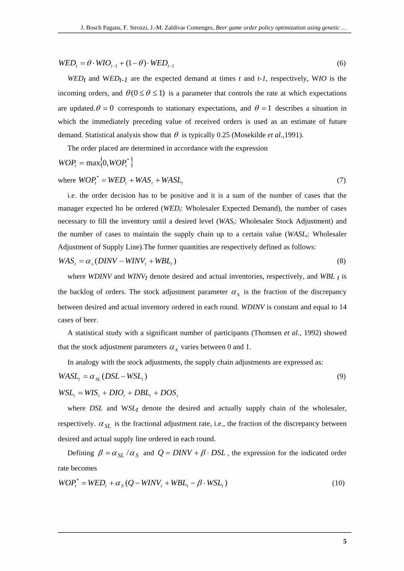
Figure 2. Effective inventory i.e. the number of cases in the stock (upper layer) and order placed (lower layer) of retailer (continuous line), wholesaler (dashed line), distributor (dotted line) and factory (continuous pointed line). Same order policy. Customer demand changes from 4 to 8 cases of beer per week in the fifth week. θ= 0.250, Q=

17, optimal parameters: αS= 0.317 and β = 0.016.

Figures 2 an 3 show the effective inventory (inventory-backlog) and order rate evolutions of

the four sectors over 60 weeks simulations using the optimal order parameters obtained with

GA considering the four sectors having same and different ordering policies, respectively. In

both cases, the effective inventories initially decrease and afterwards present a set of oscillations

that increase from retailer to factory. This behaviour is a result of the change of the customer

order rate at week 5 from 4 to 8 cases of beer. This fact produces an increase of the orders

placed by the retailer that propagates wavelike through the supply chain in the direction of the

factory producing the inventories depletion and the successive increase of the order rates to

fulfil the generated backlogs. Once the backlogs are satisfied, the inventories increase because

of the increase in the order rates, especially noticeable on sectors close to factory.


10

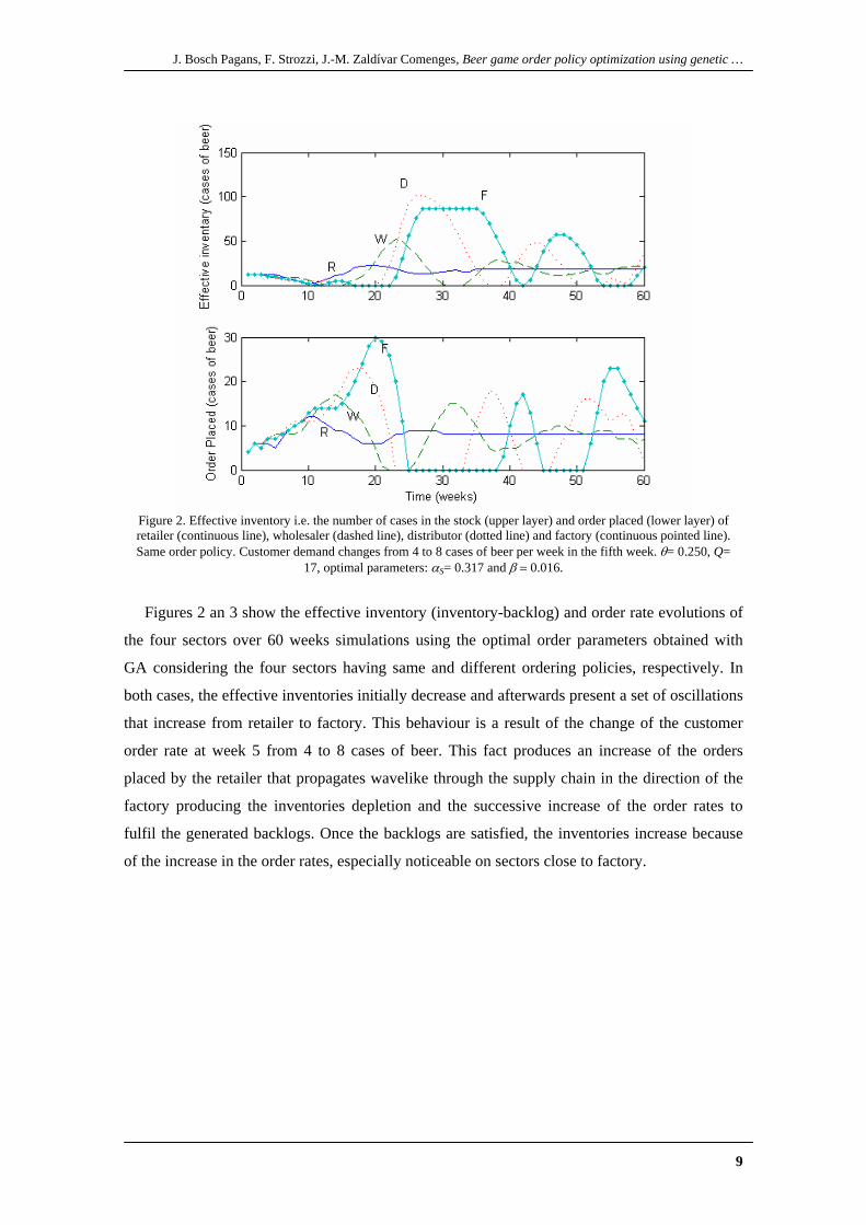
Figure 3. Effective inventory (upper panel) and order placed (lower panel) evolutions of Retailer (continuous line),

Wholesaler (dashed line), Distributor (dotted line) and Factory (continuos pointed line) with different order policies. θ = 0.250, Q = 17, optimal parameters: αR = 0.09400, βR =0.2570, αW= 0.9790, βW = 0.5910, αD= 0.9910,

βD = 0.6320, αF= 0.9600 and βF = 0.2470. Customer demand changes from 4 to 8 cases.

Mosekilde et. al, (1991) shown analytically that the fitness function J has a global minimum,

when β=0.6. The discrepancy with our results using GAs (β=0.016) can be due to the flatness of

surface J near β=0.6 that implies that GAs algorithm is very slow and stops before the analytical

minimum because some tolerances are reached. Anyway it is well known that GAs do not

always finds the best solution, but a “enough good” solution in the sense that the fitness

function assumes one of its lowest local minima. Another aspect of GAs to observe is that they

give no information about the stability of the minimum. In the case in which the participants

apply the same policy, the minimum founded is surrounded by many others minima and than a

small change in the policy can give rise to very different score. The analytical solution is placed

in stable.

When the four sectors have different order policies the inventory of the participants presents

lower and smoother oscillations and in particular distributor effective inventory is always

beyond twenty units.

In the first scenario the fitness function i.e. the final score is €2972.5, whereas in the second

scenario is €1056. In the first scenario the retailer is the sector with the lowest score, €434,

while wholesaler, distributor and factory have a score of €499, €884.5 and €1155, respectively.

On the other hand, in the second scenario, the sector with the lowest score is the distributor,

€194, and the other sectors present scores not very different. This is because all sectors


11

accomplish to contain their effective inventories when the customer order rate increases. That is

to say, there is not a clear winner as in the first scenario, but all sectors reach the objective to

keep low inventories and to avoid backlogs.

Figures 4 and 5 show the best solutions obtained from ten runs for the four sectors operating

the same and different orders policies, respectively. In the first case, solutions are

homogeneously distributed on two close zones both with small values of αS and β. The best

order policy i.e. the one with the minimum score, corresponds to αS= 0.324 and β= 0.021.

Figure 4. Solutions (crosses) obtained from ten runs of GA algorithm after 200 generations considering one order

policy in the αS - β space.

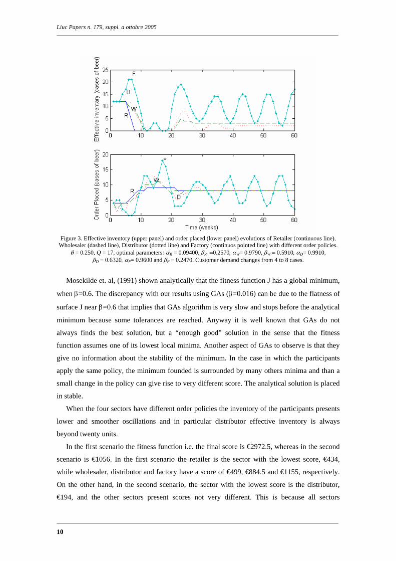
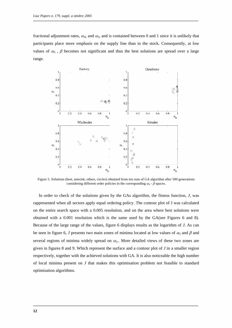
In the second scenario, solutions appear to be placed on certain regions of the parameter

space depending on the involved sector, moreover they are wider distributed as the involved

sector is farther from the factory on the supply chain. Retailer best solutions are located on low

values of αS (smaller than 0.2) it means that retailer has to adjust the stock slowly. On the

contrary, the suggestion for the wholesaler is to have αS bigger than 0.2 than it has to be quicker

than retailer in adjusting the stock and β values concentrated near 0.6. Distributor and Factory

have to be both very quick in adjusting inventory (αS near one) but Factory has to be slower

than Distributor in adjusting the supply chain.

The optimal β values increase as sectors are farther from the Factory, i.e. the production

source, as it can be seen in Figure 5 for the Factory, Distributor and Wholesaler. This fact is not

observed for the retailer sector because of the definition of β and those retailer solutions present

low αS values. As previously stated, β is the relation between the supply line and the stock


12

fractional adjustment rates, αSL and αS, and is contained between 0 and 1 since it is unlikely that

participants place more emphasis on the supply line than in the stock. Consequently, at low

values of αS , β becomes not significant and thus the best solutions are spread over a large

range.

Figure 5. Solutions (best, asterisk; others, circles) obtained from ten runs of GA algorithm after 500 generations

considering different order policies in the corresponding αS - β spaces.

In order to check of the solutions given by the GAs algorithm, the fitness function, J, was

rappresented when all sectors apply equal ordering policy. The contour plot of J was calculated

on the entire search space with a 0.005 resolution, and on the area where best solutions were

obtained with a 0.001 resolution which is the same used by the GA(see Figures 6 and 8).

Because of the large range of the values, figure 6 displays results as the logarithm of J. As can

be seen in figure 6, J presents two main zones of minima located at low values of αS and β and

several regions of minima widely spread on αS.. More detailed views of these two zones are

given in figures 8 and 9. Which represent the surface and a contour plot of J in a smaller region

respectively, together with the achieved solutions with GA. It is also noticeable the high number

of local minima present on J that makes this optimisation problem not feasible to standard

optimisation algorithms.


13

Figure 6. Contour plot of log(J) considering one ordering policy in the αS - β space.

Figure 7. Surface plot of J of the area containing the lower values in the αS - β space.


14

Figure 8. Contour plot of J considering one ordering policy in the αS - β space and obtained solutions with GA (white

circles and white star for best one).

6. Conclusions

In the present study, the optimal parameters for the order policy of the beer game for 60

weeks simulations have been obtained using GA in two different scenarios. These scenarios

consider the sectors having identical and different order policies. The search of the optimal

solution has been performed using Genetic Algorithms (Holland, 1975) due to the complexity of

the objective cost function, which has many local minima and, in the case of different policies,

many parameters.

Results have shown that best performance is obtained when sectors have different order

policies rather than having the same. Furthermore, the first case leads to a situation where only

one sector reaches the objective to have minimal inventory fluctuations and backlogs, while in

the second scenario all sectors reach this objective. The results is not surprising because in the

second case we have more parameters and than more possibilities to find good solutions.

In the first case, the optimal order policy was found on low values of αS and extremely low

of β. This combination of parameters results in a slow stock adjustment policy with carelessness

of placed orders. Despite the fact that these parameters were found to be the optimal in the


15

search space, the chain still presents large oscillations on the effective inventories due to the

customer order rate increase. Anyway this solution does not correspond to the analytical one

founded by Mosekilde et al. (1991) which find the optimum near β=0.6. The discrepancy with

our results using GAs (β=0.016) can be due to the flatness of surface J near β=0.6 that implies

that GAs algorithm is very slow and stops before the analytical minimum since some tolerances

are reached. In any case, it is well known that GAs do not always finds the best solution, but a

“enough good” solution in the sense that the fitness function assumes one of its lowest local

minima.

Having different order policies leads to an optimal solution that faces the order rate increase

of the customer keeping the inventories within desired bounds without large fluctuations and

with minimal backlogs. This is achieved by three factors that may be summarised as:

− A retailer sector with low values of αS that responds to the customer order rate increase

with still adjustments. This fact avoids the propagation of the customer order rate

increase wavelike through the chain as observed in the other scenario.

− A factory sector with high values of αS that permits to deliver constantly without delays

due to depletion of its inventory.

− An increasing importance of the orders placed as involved sectors are farther from the

factory that avoids over-ordering, and thus the amplification of order rate increase

through the chain.


16

References

Chen, F., Z., Drezner, J. K., Ryan, D. Simchi-Levi (2000). Quantifying the Bullwhi

Effect in a Simple Supply Chain: The impact of Forecasting, Lead Times, and Information, Management Science, 46, 436-443.

Davis, H. L., Hoch, S. J.& E. K. Eqaston Ragsdale, E.K. (1986). An Anchoring and adjustment model of spousal predictions. Journal of Consumer Research, 13, 25-37

Einhorn, H. J.& Hogarth, R. M. (1985). Ambiguity and Uncertainty in probabilistic inference, Psychological Rewiev, 92, 433-461.

Holland, J. H. (1975). Adaptation in Natural and Artificial Systems. Cambridge: MIT Press.

http://cs.felk.cvut.cz/~xobitko/ga/

http://www.rennard.org/alife/english/gavintrgb.html

Jarmain, W.E. (1963). Problems in Industrial Dynamics. Cambridge: MIT Press.

Lagarias, J.C., Reeds, J. A., Wright, M. H. & P.E. Wright, P. E. (1998). Convergence Properties of the Nelder-Mead Simplex Method in Low Dimension. SIAM Journal of Optimization, 9 (1), 112-147.

Mosekilde, E. and Larsen, E.R. (1998) Deterministic Chaos in the Beer Production-Distribution Model, Syst. Dyn. Rev. 4, 131-147.

Mosekilde, E., Larsen, E. & Sterman, J. D. (1991). Coping with Complexity: Deterministic Chaos in Human Decision Making Behaviour. In “Beyond Belief: Randomness, Prediction and Explanation in Science,” J.L. Casti and A. Karlqvist (eds.), CRC Press, Boca Raton.

Sterman, J. D. (1988). Deterministic Chaos in Models of Human Behaviour: Methodological Issues and Experimental Results. System Dynamics Review, 4, 148-178.

Sterman, J.D. (1989). Modelling Managerial Behaviour: Misperceptions of feedback in a Dynamic Decision Making Experiment. Management Science 35, 321-339.

Thomsen, J.S., Mosekilde, E. & Sterman, J.D. (1992). Hyperchaotic Phenomena in dynamic decision making. Syst. Analysis Modelling Simulation, 9, 137-156.

Yen-Zen Wang (2003), Using genetic algorithm methods to solve course scheduling problems. Expert System with Applications, 25, 39-50.

Zhanybay, T., Zhusubaliyev & Mosekilde, E., (2003) Bifurcations and Chaos in piecewise-smooth dynamical systems. World Scientific.

beer game order policy optimization using genetic algorithms · beer game order policy optimization...

Documents