1

Bangor Business School

Working Paper (Cla 24)

BBSWP/13/010

RATIONALIZING THE VALUE PREMIUM IN EMERGING MARKETS

By

M. Shahid Ebrahim*, Sourafel Girma**, M. Eskander Shah***, Jonathan Williams*

September, 2013

* Bangor Business School

Bangor University

Hen Goleg

College Road

Bangor

Gwynedd LL57 2DG

United Kingdom

Tel: +44 (0) 1248 382277

E-mail: business@bangor.ac.uk

** University of Nottingham, UK

*** INCEIF (International Centre for Education in Islamic Finance), Malaysia

2

Rationalizing the Value Premium in Emerging Markets

Abstract

We reconfirm the presence of value premium in emerging markets. Using the Brazil-Turkey-India-China

(BTIC) grouping during a period of substantial economic growth and stock market development, we attribute

the premium to the investment patterns of glamour firms. We conjecture based on empirical evidence that

glamour firms hoard cash, which delays undertaking of growth options, especially in poor economic conditions.

Whilst this helps to mitigate business risk, it lowers market valuations and drives down expected returns. Our

evidence supports arguments that the value premium is explained by economic fundamentals rather than a risk

factor that is common to all firms.

JEL Classifications: G110 (Portfolio Choice; Investment Decisions), G120 (Asset Pricing).

Keywords: Asset Pricing, Growth (i.e., Glamour) Stocks, Multifactor Models, Real Options, Value (i.e.,

Unspectacular) Stocks.

3

Rationalizing the Value Premium in Emerging Markets

I. Introduction

″Growth stocks, which derive market values more from growth options, must therefore be riskier

than value stocks, which derive market values more from assets in place. Yet, historically, growth

stocks earn lower average returns than value stocks.″ (Lu Zhang, 2005, pp 67)

Fama and French’s (1992) finding, that a single factor encapsulating risk (beta) does not adequately

explain cross-sectional differences in stock returns, has motivated an important strand of research on asset

pricing, reigniting the debate on the fundamental relationship between risk and return, and challenging the

widely-accepted Capital Asset Pricing Model (CAPM). Subsequently, numerous theoretical and empirical

studies examine the cross-sectional variation in stock returns with many finding patterns unexplained by the

CAPM and commonly known as anomalies.

This paper examines one of the most pronounced anomalies, the value premium puzzle. Portfolios

formed on the basis of high book-to-market (BE/ME), cash flow-to-price (C/P) and earnings-to-price (E/P) are

reported to earn significantly higher risk-adjusted returns than portfolios with contrasting characteristics.

However, the previous literature fails to achieve a consensus on the source of the value premium (Chou et al.,

2011). The objectives of this paper are to confirm the presence of value premium in a new market, to provide a

new rationalization based on economic fundamentals, and to reconcile the diverging perspectives which are

apparent in the literature. The value premium reflects a tendency for ‘glamour firms’ to hoard cash and delay

implementation of growth strategies, particularly in times of economic uncertainty (Titman, 1985; McDonald

and Siegel, 1986; Ingersoll and Ross, 1992). Since growth (glamour) stocks derive their market value from

embedded growth in the form of real options (Zhang, 2005), we argue that cash hoarding limits their exposure to

risk but exerts a significant detrimental impact on their stock returns.

The theoretical basis for our analysis derives from Fama and French (1995) and Daniel and Titman

(1997). Fama and French (1995) develop a three-factor model, in which the factor that captures distress risk,

known as HML, is lower for growth (glamour) firms than for value firms. The debate centers on whether lower

distress risk accounts for the discrepancy in average returns between value firms and growth firms (Fama and

French, 1995) against claims that distress risk does not contribute to the value premium (Dichev, 1998; Griffin

and Lemmon, 2002). We contend that both the cash-drag factors and firm characteristics, as highlighted by

Daniel and Titman (1997), are of relevance.

In comparison with value firms, growth firms face a wider array of strategic options, carrying various

levels of risk. These firms may limit their exposure to risk by abstaining from investing resources in risky

strategies, especially in poor economic environments. Accordingly, growth firms hoard cash when economic

conditions are tough, and realize lower returns. By contrast, value firms are prominent in mature and/or

declining markets and face a more limited range of options. Such firms face financial risk, as well as business

risk, owing to a tendency to use existing assets as collateral in order to leverage earnings. They have less

flexibility in managing their risk, because past sunk-cost investment in assets is irreversible (Zhang, 2005). Our

4

approach in rationalizing the value premium is consistent with the neoclassical framework, in which low-risk

assets yield lower returns and vice versa.

Our research draws on two recent studies that contrast the approach of Fama and French (1995) with

Daniel and Titman (1997). In a similar vein to Daniel and Titman (1997), Chen et al. (2011) propose a three-

factor model incorporating factors with greater explanatory power for cross-sectional returns than the Fama and

French model. We aim to extend these findings, by obtaining results that are not sample-specific (a limitation of

Chou et al., 2011), and by adopting a real options framework in cases where the Net Present Value investment

perspective (Chen et al., 2011) is inapplicable.1 This paper is among the few that try to reconcile differences not

only between the neoclassical asset-pricing literature (Fama and French versus Daniel and Titman), but also the

neoclassical and behavioral literature.

Our application is to a new grouping of four, large emerging markets: namely, Brazil, China, India and

Turkey, the BTIC group.2 Each of these economies has achieved remarkable growth since the early 2000s,

which implies there are many firms endowed with plentiful growth options.3 Our paper addresses two research

questions: (i) is a statistically significant value premium present in the BTIC? (ii) is it possible to rationalize the

value premium and reconcile the apparently conflicting views in the literature? To investigate questions (i) and

(ii) we source relevant variables from 1999 to 2009 to allow our analysis of value anomalies to be conducted

under generally favourable economic conditions including increasing stock market integration following the

liberalization of equity markets in the BTIC.

By way of preview, we find a significant value premium in the BTIC which is not new for emerging

markets but re-emphasizes the value premium is not a developed country phenomenon. A second result, which

is based on the widely-used Altman Z-score model, shows value firms are no more prone to risk than growth

firms, but value firms employ more leverage. Our evidence suggests the investment patterns of growth firms are

the source of the value premium. In an asset-pricing model, the HML coefficients of growth portfolios are small

during low-growth periods and considerably larger during high-growth periods. This pattern is consistent with

the hypothesis that growth firms delay the implementation of new strategies in periods of economic uncertainty

in order to limit their risk. The HML coefficients of growth portfolios are sensitive to changes in size (total

assets). Accordingly growth in total assets, interpreted to proxy implementation of growth strategies, explains

1 Ingersoll and Ross (1992, p. 2) explain this as follows:

“If in making the investment today we lose the opportunity to take on the same project in the future, then the project competes with itself delayed in time. In deciding to take an investment by looking at only its NPV, the standard textbook solution tacitly assumes

that doing so will in no way affect other investment opportunities. Since a project generally competes with itself when delayed, the

textbook assumption is generally false. Notice, too, that the usual intuition concerning the “time value of money” can be quite misleading in such situations. While it is true NPV postponing the project delays the receipt of its positive NPV, it is not true that we

are better off taking the project now rather than delaying it since delaying postpones the investment commitment as well.

Of course, with a flat, non-stochastic yield curve we would indeed be better off taking the project now, and this sort of paradox could not occur. But that brings up the even more interesting phenomenon that is central focus of this article, the effect of interest-rate

uncertainty on the timing of investment”.

2 Non-availability of data for Russia precludes investigation of the BRIC quartet (Brazil, Russia, India and China). We select Turkey

as an alternative large European emerging economy, and note the creator of the BRIC acronym, Jim O’Neill, plans to include Turkey

and three other emerging economies in a new grouping (Hughes, 2011).

3 The rapid growth of emerging economies, and the impact on the world economy, is discussed extensively in the popular press. For

instance, the August 6th, 2011 issue of the Economist magazine highlights several noteworthy statistics on emerging versus developed economies. In 2010 emerging economies account for nearly 54% of world Gross Domestic Product (GDP) measured at purchasing

power parity and 75% of global real GDP growth over ten years. Exports exceed 50% of the world total, and imports account for 47%. Foreign direct investment (FDI) to emerging economies significantly increased recently as have commodity consumption and capital spending. Stock market capitalization equals 35% of the world total, this share having tripled since 2000.

5

the change in business risk of growth firms. This affirms our hypothesis that the investment patterns of growth

firms impact significantly on their risk and return.

Our results also resolve the various perspectives in the literature in three ways. First, Fama and French

(1995) and Daniel and Titman (1997) attribute the outperformance of value stocks to different causes. Daniel

and Titman (1997) explain performance differentials between value and growth stocks as being due to the

characteristics of firms as opposed to covariance with risk factors. Value stocks outperform because growth

firms tend to hoard cash and delay undertaking the growth options they are endowed with and this drags down

their returns. In the Fama and French (1995) framework, this phenomenon is attributed to distress risk. Second,

growth firms’ flexibility to manage their embedded growth options to their operational and strategic advantage

yields not only profit, but also provides utility in its own right: embedded options provide ‘glamour firms’ with

an allure with which to entice investors. ‘Fascination’ with growth firms (Sargent, 1987) creates a premium in

price (and hence a discount in returns), which helps reconcile the neoclassical and behavioral perspectives.

Third, the over-reaction hypothesis of DeBondt and Thaler (1985 and 1987) is rationalized through the volatile

nature of value firms’ leveraged equity, which is akin to Call options. These options are depressed in poor

economic states but rebound in prices with improving economic climate.

This paper is organized as follows. Section II reviews the relevant literature, and identifies the research

questions and methodology. Section III offers a brief synopsis of market developments in the BTIC. Section IV

presents data and methodology. The results and checks for robustness are in Sections V and VI. Section VII

offers concluding comments.

II. Literature Review

The Capital Asset Pricing Model (CAPM) posits that risk, measured using beta, accounts for the cross-

section of expected stock returns (Sharpe, 1964; Lintner, 1965a,b; Mossin, 1966). Numerous empirical studies

test the model, on the assumption that beta is the sole explanatory variable with a positive and linear relation to

asset return, yet results are inconclusive. Several early empirical studies (Black et al., 1972; Blume and Friend,

1973; Fama and McBeth, 1973) provide support for the CAPM. Later studies, however, are more critical, citing

evidence of anomalies and questioning the validity of the assumptions (Roll, 1977; Basu, 1977, 1983; Stattman,

1980; Banz, 1981; DeBondt and Thaler, 1985; Rosenberg et al., 1985; Bhandari, 1988; Jegadeesh and Titman,

1993; Cohen et al., 2002; Titman et al., 2004). Fama and French (1992) conclude that CAPM with a single

factor does not adequately explain cross-sectional stock returns, and propose a three-factor model to capture the

multidimensional aspect of risk, comprising: (i) a market factor (RM-Rf); (ii) a size premium (SMB) (return on a

portfolio of small stocks minus return on a portfolio of large stocks); and (iii) a value premium (HML) (return

on a portfolio of value stocks with high BE/ME minus return on a portfolio of growth stocks with low BE/ME).

This approach builds on Merton’s (1973) intertemporal CAPM and Ross’s (1976) arbitrage pricing theory

(APT). Fama and French (1993, 1995) show SMB and HML are related to risk factors in stock returns; and

both factors contain explanatory power for the cross-sectional variation in stock returns.

The three-factor model has attracted a great deal of academic interest, much of it centered on the source

of the value premium. In line with the hypothesis of rational pricing, Fama and French (1993) and Chen and

6

Zhang (1998) suggest value firms are riskier and more likely to be subject to financial distress than growth

firms. Fama and French (1995) demonstrate that value [growth] stocks are generally associated with

persistently low [high] earnings, creating a positive [negative] loading on HML, which implies higher [lower]

risk of distress. On the contrary, Zhang (2005) claims value firms are riskier because their assets at risk are

larger than those of growth firms. This becomes particularly evident in poor economic environments, where

firms with fixed assets pose greater risks for investors than those with growth options. Value firms are burdened

with unproductive capital that cannot be liquidated in order to recover the cost of the original investment.

More recent value premium studies investigate how differing states of the world affect the strength of the

premium. The empirical evidence contained in these papers demonstrates the value premium is time varying

and sensitive to changes in economic conditions. Stivers and Sun (2010) show the value premium is

countercyclical and higher during periods of weak economic fundamentals whereas Guo et al. (2009) find value

stocks are riskier than growth stocks under weak economic conditions. Similarly, expected excess returns on

value stocks are more sensitive to deteriorating economic conditions during episodes of high market volatility

(Gulen et al., 2011). Finally, the size of the value premium positively relates to its conditional volatility (Li et

al., 2009).

Several alternative theories also seek to explain the value premium. Focusing on investor sentiment and

trading strategies, Lakonishok et al. (1994) and Haugen (1995) attribute a tendency for value (‘unspectacular’)

firms to produce superior returns to an irrational tendency on the part of investors to extrapolate the past strong

[weak] performance of the growth [value] firm into the future. Investors overbuy [oversell] the growth [value]

firm’s stock. Lower [higher] than expected realized performance on the part of the growth [value] firm

generates a low [high] stock return.4 Similarly De Bondt and Thaler (1985, 1987) observe that poorly

performing stocks (‘losers’) over the past three-to-five years outperform previous ‘winners’ during the

subsequent three-to-five years.

Daniel and Titman (1997) claim the explanation for the value premium lies in firm characteristics rather

than covariance risk. High covariance between the returns of value stocks reflects common firm characteristics,

such as, the line of business or industry classification. Daniel and Titman (1997) show high covariance between

stock returns bears no significant relation with the distress factor. Evidence of high covariance precedes any

signs of financial distress on the part of value firms.5

Other possible explanations for the value premium focus on methodological issues in empirical studies.

Banz and Breen (1986) and Kothari et al. (1995) suggest sample selection may be biased towards firms that

survived a period of distress, rather than those that failed. The notion that survivorship bias accounts for the

value premium is rejected, however, by Davis (1994), Chan et al. (1995) and Cohen and Polk (1995). Data

‘snooping’, an eventual tendency for repeated testing using the same data to reveal spurious patterns is cited as

an explanation for the value premium phenomenon (Lo and MacKinlay, 1988; Black, 1993; MacKinlay, 1995;

Conrad et al, 2003). Any such tendency might be mitigated by testing data from different periods or countries

(Barber and Lyon, 1997).

4 La Porta et al. (1997) find value firms enjoy a systematically positive earnings surprise while glamour firms display the opposite.

5 Lee et al. (2007) find stock characteristics better explain UK value premiums.

7

In spite of contentions that the value premium is a developed country phenomenon (see Black, 1993;

MacKinlay, 1995; Campbell, 2000) other evidence supports the proposition of a value premium in emerging

markets. In samples containing some (or all) of the BTIC group, Rouwenhorst (1999) uses a cross section

analysis of returns across twenty emerging markets between 1982 and 1997, whereas Barry et al (2002) study 35

emerging markets from 1985 to 2000. De Groot and Verschoor (2002) confirm the value premium for a sample

of south east Asian markets between 1984 and 2000. Ding et al (2005) also examine markets in south and east

Asia. Their study recognizes cross country differences with respect to the value premium, but unfortunately the

data it uses end prior to the Asian crisis of 1997, which is a major drawback as more recent value premium

studies suggest the premium may change in an economic downturn. Given the very limited work on explaining

the value premium in the context of emerging markets, many questions surrounding the value premium remain

unanswered. This paper will test for the value premium during the most recent period of growth in emerging

markets whilst offering a cross country perspective and it will also analyse the source of the premium in

emerging markets, which few papers undertake.6

III. Market developments in the BTIC

The BTIC countries liberalized their stock markets between the late 1980s and mid-1990s. The benefits

of liberalization include higher levels of real economic growth and real investment (Bekaert et al., 2003a) with

studies reporting a significant relationship between stock market liquidity and economic growth (Levine and

Zervos, 1998). Liberalization is expected to increase the level of integration between emerging stock markets

and the world market which should lower country risk premiums. In the 1990s emerging markets represented a

new asset class and stock prices in those markets were driven upwards by investors seeking to diversify their

portfolios, leading to permanently lower costs of capital in the emerging markets (Bekaert and Harvey, 2003).

Several studies propose methods to effectively date when liberalization takes place (see, Bekaert et al, 2003b;

Kim and Kenny, 2007).7 We calculate several indicators to proxy stock market development and growth in the

BTIC (Source: World Development Indicators). In 2010, the BTIC share of global stock market capitalization

equals 15.10% (US$ 8 trillion) increasing by nearly five-fold since the 2000 level of 3.18%. The ratio of listed

firms’ market capitalization-to-GDP measures the level of stock market deepening and it shows the combined

BTIC stock market is nearly two times deeper in 2010 compared to 2000 (78.47% c.f. 39.66%). Similarly, the

BTIC stock markets are more liquid as measured by the ratio of value of stocks traded-to-GDP. Taking 1992 as

a year to represent pre-stock market liberalization, liquidity increases by a factor of eight in Brazil (42.09% in

2010); over thirty four in China (135.40% in 2010); almost nine in India (62.74% in 2010); and over eleven in

Turkey (57.66% in 2010).

IV. Data and Methodology

We source data on listed firms in Brazil, Turkey, India and China for the period 1999 to 2009 from

DataStream. The sample firms meet standard criteria employed widely in the literature: stock prices are

6 One exception is a study of Singapore that attributes the value premium to a one-way overreaction of value firms (Yen et al., 2004).

7 The year of equity market liberalization in the BTIC is as follows: Brazil, 1991; China, 1995; India, 1992; and Turkey, 1989 (Kim and Kenny, 2007).

8

available for December of year t-1 and June of year t, and book value for year t-1; and each firm has at least two

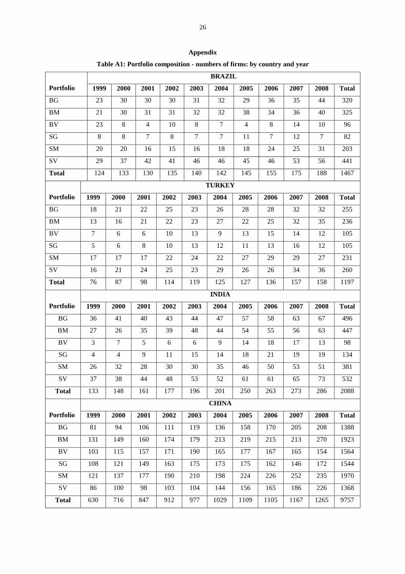
years’ complete data.8 Table A1 in the Appendix shows the number of firms belonging to each portfolio by

country and year.

In order to identify the existence of a value premium, we employ the standard Fama and French (1993)

methodology. We form six portfolios (S/L, S/M and S/H; B/L, B/M and B/H) by intersecting two groups that

are arranged by ME = market value of equity, and BE/ME where BE = net tangible assets (equity capital plus

reserves minus intangibles). Stocks with ME higher than the median are classified as ‘big’ (B); those with ME

below the median are classified ‘small’ (S). For BE/ME the three breakpoints are bottom 30% (‘Low’), middle

40% (‘Medium’) and top 30% (‘High’).9 We calculate value-weighted monthly returns for the six portfolios

from July of year t to June of year t+1, when we re-form the portfolios.

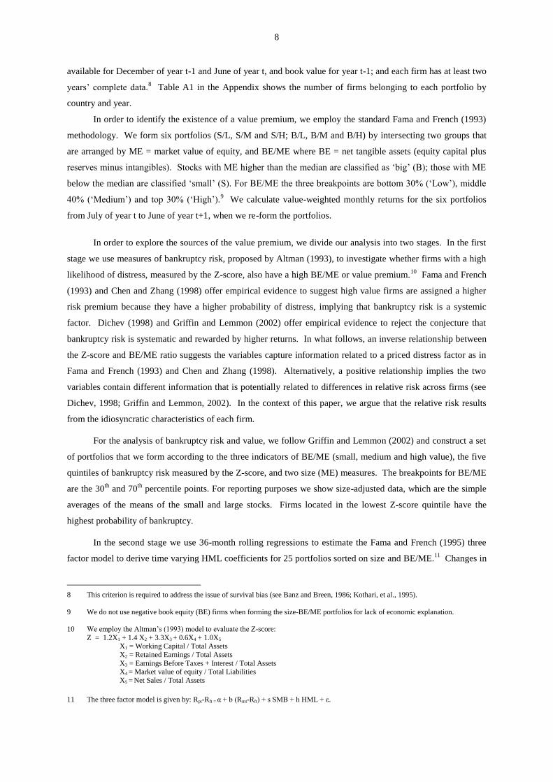
In order to explore the sources of the value premium, we divide our analysis into two stages. In the first

stage we use measures of bankruptcy risk, proposed by Altman (1993), to investigate whether firms with a high

likelihood of distress, measured by the Z-score, also have a high BE/ME or value premium.10

Fama and French

(1993) and Chen and Zhang (1998) offer empirical evidence to suggest high value firms are assigned a higher

risk premium because they have a higher probability of distress, implying that bankruptcy risk is a systemic

factor. Dichev (1998) and Griffin and Lemmon (2002) offer empirical evidence to reject the conjecture that

bankruptcy risk is systematic and rewarded by higher returns. In what follows, an inverse relationship between

the Z-score and BE/ME ratio suggests the variables capture information related to a priced distress factor as in

Fama and French (1993) and Chen and Zhang (1998). Alternatively, a positive relationship implies the two

variables contain different information that is potentially related to differences in relative risk across firms (see

Dichev, 1998; Griffin and Lemmon, 2002). In the context of this paper, we argue that the relative risk results

from the idiosyncratic characteristics of each firm.

For the analysis of bankruptcy risk and value, we follow Griffin and Lemmon (2002) and construct a set

of portfolios that we form according to the three indicators of BE/ME (small, medium and high value), the five

quintiles of bankruptcy risk measured by the Z-score, and two size (ME) measures. The breakpoints for BE/ME

are the 30th

and 70th

percentile points. For reporting purposes we show size-adjusted data, which are the simple

averages of the means of the small and large stocks. Firms located in the lowest Z-score quintile have the

highest probability of bankruptcy.

In the second stage we use 36-month rolling regressions to estimate the Fama and French (1995) three

factor model to derive time varying HML coefficients for 25 portfolios sorted on size and BE/ME.11

Changes in

8 This criterion is required to address the issue of survival bias (see Banz and Breen, 1986; Kothari, et al., 1995).

9 We do not use negative book equity (BE) firms when forming the size-BE/ME portfolios for lack of economic explanation.

10 We employ the Altman’s (1993) model to evaluate the Z-score:

Z = 1.2X1 + 1.4 X2 + 3.3X3 + 0.6X4 + 1.0X5

X1 = Working Capital / Total Assets

X2 = Retained Earnings / Total Assets

X3 = Earnings Before Taxes + Interest / Total Assets X4 = Market value of equity / Total Liabilities

X5 = Net Sales / Total Assets

11 The three factor model is given by: Rpt-Rft = α + b (Rmt-Rft) + s SMB + h HML + ε.

9

the loading over time reflect changes in business and financial risk. Subsequent analysis uses the estimated

HML coefficients on growth and value portfolios as dependent variables. HML is interpreted to proxy firm

characteristics which implies common variation in returns arises because individual portfolios comprise similar

stocks with similar factor loadings irrespective of whether a firm is distressed or not. This interpretation follows

Daniel and Titman (1997) and it contrasts the view of Fama and French (1993) that HML is proxy for distress

probability. A preliminary analysis shows the Fama and French (1995) model provides an adequate description

of portfolio returns for each of the BTIC since none of the estimated alpha coefficients are significantly different

from zero (see Table 1).12

[Insert Table 1 here]

We use panel data models to estimate the time-varying coefficient on HML for the i’th portfolio at time t

on a set of conditioning variables known at time t. The conditioning variables are the current and lagged values

of the natural logarithms of total assets and total debt. The assets variable captures the sensitivity of the

coefficient on HML to growth whilst the debt variable measures sensitivity to leverage. GDP growth controls

for macroeconomic conditions. Interaction variables allow for differences in the coefficients for value and

growth portfolios. A Hausman test selects between fixed-effects and random-effects models.

V. Empirical Results

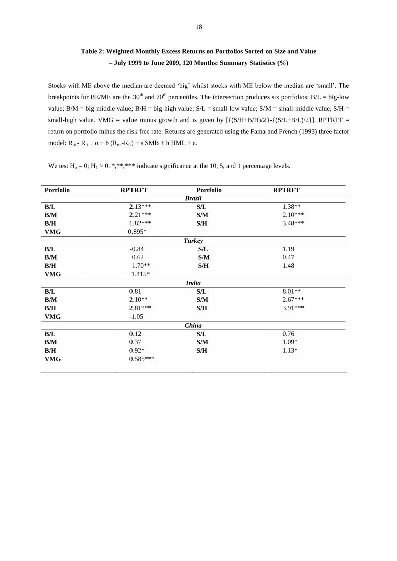
Table 2 reports the weighted monthly excess returns of the six size-BE/ME portfolios constructed using

the three factor model (Fama and French, 1993) for each of the BTIC. For portfolios constructed using “big”

stocks, we find statistically significant excess returns to value firms in excess of returns to growth firms in

Turkey, India and China. In Brazil, excess return is highest for the intermediate band. For portfolios constructed

using “small” stocks, excess returns are significant and higher for value firms in Brazil and China. Although

this pattern repeats in Turkey the returns are not significant. In contrast, returns are significant and highest for

growth firms in India. A positive and significant VMG (value minus growth) confirms the findings for Brazil,

Turkey and China. VMG measures the difference in excess returns between value and growth portfolios and

equals (B/H+S/H)/2–(B/L+S/L)/2. Our evidence infers the existence of a value premium in each country except

India. We conjecture the fast-growing information technology industry in India, containing many small high-

technology firms, might account for the exceptionally high excess return in the SG portfolio.

[Insert Table 2 here]

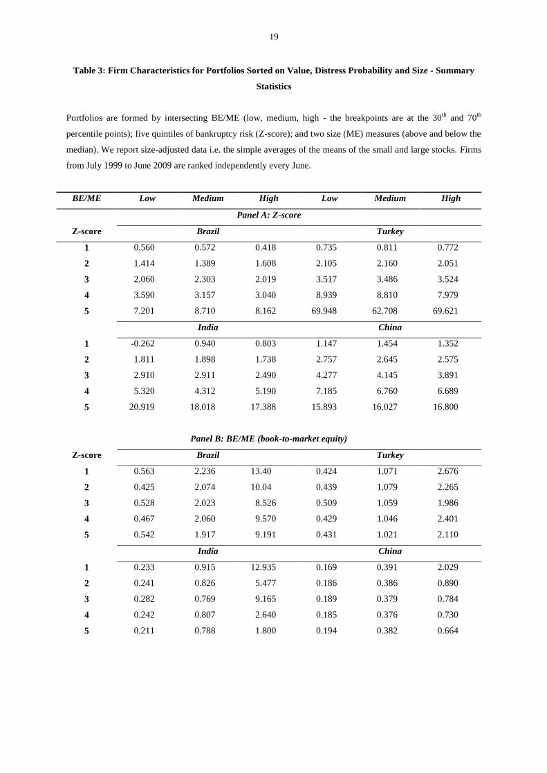
In Table 3 we construct the portfolios as follows. Portfolios are sorted into small and large categories,

and interlocked with value (using breakpoints at the 30th

and 70th

percentile points to define low, medium and

high value) and the probability of bankruptcy as indicated in quintiles of Z-scores. Table 3 reports size-adjusted

data, the simple average of small and large stocks, for bankruptcy risk, size, returns, and leverage.

Panel A shows little variation in the mean Z-scores between low value and high value portfolios in each

country except for Indian firms in quintile one for low value stocks (-0.262) relative to their high value

12 The average value of beta is different from one depending on the orientation of firms in the economy. If the aggregate firm in the

economy is value oriented then beta will be less than 1. This is consistent with studies which demonstrate that stocks with below

market risk (low beta) yield higher risk adjusted return than predicted by the theoretical CAPM (see Black et al., 1972; Miller and Scholes, 1972), and evidence showing value firms have lower beta than growth firms (see Capaul et al., 1993).

10

counterparts (0.803). The lowest (highest) Z-scores are in Brazil (Turkey). In the higher quintiles and across

countries, low and high values stocks achieve similar Z-scores, which suggest the presence of value premium is

not related to distress risk thereby contradicting Fama and French (1995). Panel B shows the average book-to-

market ratio of the three stock groupings by quintiles of Z-score. On average in Brazil, India and China, high

value firms in the lowest quintile achieve considerably larger book-to-market ratios, which again is inconsistent

with the Fama and French hypothesis.

[Insert Table 3 here]

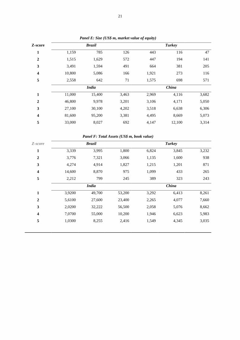
Table 3 also reports statistics on profitability, leverage, size (capitalization), and total assets for firms in

each portfolio in order to further examine the hypothesis that the Z-score and BE/ME are related to

characteristics purported to reflect distress risk. Panel C shows mean profitability is positively related to the Z-

score, and is larger for high value firms in each country (except Turkey). Leverage is inversely related to the Z-

score in each country (see Panel D). The data show high value and high risk firms are more heavily levered

particularly in Brazil and India, which supports our earlier argument that value firms use more debt financing

than growth firms. In Brazil and Turkey, low value stocks tend to be better capitalized (see Panel E) and larger

in terms of total assets whereas high value firms are larger in terms of assets size in China and India (see Panel

F).

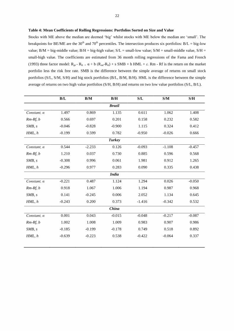
Table 4 shows the results of rolling regressions estimations of the Fama and French three factor model

for the six portfolios. Since our focus is on the coefficient of HML (h), we do not discuss other coefficients.

HML is defined as the difference between the simple average returns on two high value portfolios (S/H and

B/H) and two low value portfolios (S/L and B/L). All B/M portfolios (except China), B/H and S/H portfolios

are associated with positive values on HML. That we observe positive loadings on value-orientated portfolios in

each country demonstrates the presence of the value premium in those markets. We observe negative

coefficients on HML for low value portfolios B/L and S/L across countries, and also for portfolio S/M (except

Turkey). The findings demonstrate a difference in returns between portfolios of growth stocks ranked by firm

size.

[Insert Table 4 here]

In spite of the apparent heterogeneity in loadings, our findings - at least for Brazil and China - are

consistent with the contention of Fama and French (1995) that growth [value] stocks should have negative

[positive] loadings. In contrast to Fama and French (1995) but consistent with Daniel and Titman (1997), we

suggest the negative loading on growth firms is not a function of distress as our earlier analysis indicates the

level of distress is comparable for growth and value firms. Rather, we that contend growth portfolios have

lower loadings because the choice of delaying growth options gives growth firms the opportunity to reduce their

risk. In addition, delaying the exercise of these options enables growth firms to accumulate and/or hoard cash.

Our results offer support for claims that growth portfolios earn low returns because of a cash drag effect since

cash generates very little return.

We contend that investors display an ‘infatuation’ with growth firms based on the potential growth

opportunities stemming from embedded growth options. Thus, stock prices are driven upwards through bidding

which contrasts with the ‘unspectacular’ value firms. In Lucas’ Rational Expectations framework (1978),

11

growth firms constitute an ‘alluring’ asset, a point further extended by Sargent (1987). This interpretation

reconciles the neoclassical and behavioral perspectives. The leverage of value firms causes a drag on their

performance in poor economic environments particularly as leveraged equity displays volatility associated with

financial options (see Merton, 1974). The expansion of the economy creates a bounce-back effect on value

stocks, helping to reconcile the neoclassical perspective with the behavioral as espoused by DeBondt and Thaler

(1985, 1987).

In light of our intuition, we graph the coefficients of HML for twenty of the 25 portfolios to provide

further insight to our argument.13

Figure 1a-d illustrate the patterns of time varying betas (coefficients of HML)

for growth and value portfolios. The figures, with the exception of Turkey, demonstrate that value portfolios

have higher beta and are more stable over time compared to growth portfolios.

[Insert Figure 1a-d here]

The exercise we report on above uses rolling regressions to estimate the three factor model. To check the

robustness of the results, we re-estimate the models using static panel data techniques. A Hausman test finds the

χ2 statistic equal to 38.48 and statistically significant at the 1 percent level. The test result shows the fixed

effects model is preferred to its random effects counterpart. Table 5 reports the fixed-effects estimation.

Ex ante we expect growth portfolios to exhibit sensitivity to size (total assets) whereas value portfolios

should display sensitivity to leverage. Using a binary variable to identify value portfolios, we create interaction

variables between this indicator and size and leverage, at contemporaneous and lagged values for two periods to

determine separate value portfolio effects. Lastly, the natural logarithm of GDP growth controls for business

cycle effects.

The results show a positive and significant relation between HML and total assets lagged two periods at

the 10 per cent significance level. However, the estimated coefficients on the interaction variables with total

assets (6 and 8) are negatively signed and statistically significant (except 7 the coefficient on the one period

lag interaction). The finding confirms the differential between value and growth portfolios in terms of the

sensitivity of HML with respect to size. The estimated coefficient on leverage is negative (though insignificant)

and suggests more highly levered portfolios are less sensitive. However, the interaction term between

contemporaneous leverage and HML (9) is positive and highly significant, which signals value portfolios are

very sensitive to leverage.

[Insert Table 5 here]

VI Robustness

We use an alternative procedure to construct portfolios to test the robustness of the results and construct

twenty five intersecting size-value portfolios using the quintile breakpoints for ME and BE/ME and equally

weighted monthly returns instead of value-weighted returns. To illustrate, using ‘S’ to indicate size and ‘L’ to

indicate BE/ME, the portfolio S1L1 contains stocks that are ranked in the first quartile (less than 20%) of both

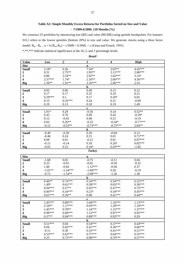
size and value. Table A2 in the Appendix presents the data for the 25 portfolios and confirms the finding in

13 We categorize portfolios labelled with L1 and L2 as growth portfolios and L4 and L5 as value portfolios. Portfolios labelled with L3

are not graphed because they are neither growth nor value. In Figure 1a-d we present four graphs per country rather than 25. The remainder are available from the authors upon request.

12

Table 1 which demonstrates the Fama and French (1995) model adequately describes the portfolio returns.

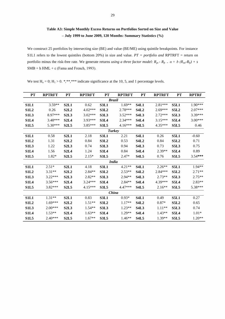
Table A3 reports the simple excess returns on the 25 portfolios by country and checks the robustness of findings

reported in Table 2. The distribution of excess returns across portfolios lets us formulate some generalizations:

first, excess returns on the highest value firms tend to be greater in comparison with low value firms; second, the

distinction in returns by size is less marked and varies across countries. Table A3 shows the smallest firms

achieve significant returns, which for some portfolios, exceed returns on larger firms. Both sets of our results

confirm findings from several previous studies that show high value stocks achieve larger mean expected

returns. In Table A4 we report robustness checks for findings in Table 4 using the set of 25 interlocking

portfolios. The estimated HML coefficients exhibit intra and inter heterogeneity across the BTIC although some

generalized country specific patterns are apparent. For instance, the value premium is supported by the positive

loadings for medium-to-large sized and medium-to-high value portfolios in Brazil (except for the portfolio

containing the largest and highest value stocks). In the case of China, we observe positive loadings for a limited

number of portfolios, namely, portfolios of mid-to-large sized firms in the upper two quartiles of value. The

loadings on portfolios in India and Turkey are all positive (with two exceptions for Turkey) yet it is difficult to

discern hard patterns across size and value quintiles. Lastly, we observe the magnitude of loadings for India and

Turkey to be greater relative to Brazil and China.

VII Conclusion

A number of theories are postulated to rationalize the source of the value premium yet the issue remains

controversial. We reassess this issue for the BTIC group of countries that are characterized as having vast

economic potential. The paper rationalizes the value premium in terms of economic fundamentals, attributing

the premium to the investment patterns of growth firms that we contend are more likely to hoard cash,

particularly during episodes of economic malaise. Although this behaviour is understood because it limits

growth firms’ exposure to risk, nevertheless it negatively impacts on both their market valuation and returns.

The paper helps to reconcile the diverging neoclassical views of Fama and French (1995) and Daniel and

Titman (1997) in explaining the expected returns of value and growth stocks. Fama and French (1995) claim the

HML coefficient measures distress risk whereas Daniel and Titman (1997) believe it captures firm

characteristics. Our evidence offers support for the latter interpretation. We contest that growth firms are

endowed with growth options, which entails capital outlay whilst enhancing business risk and it is this feature

that differentiates growth firms from value firms. Value firms, by contrast, use fixed assets as collateral to lever

up in order to boost earnings, which in turn aggravates financial risk. This interpretation of our findings is

consistent with Chen et al. (2011).

We also reconcile the diverging neoclassical and behavioral perspectives by invoking a rational

expectations perspective (Lucas, 1978) as extended by Sargent (1987). We consider the range of options

available to growth firms provides a utility (‘infatuation’) that is separate from monetary returns in the forms of

capital gains and dividends. This inherent utility of growth firms is attractive to investors and causes their stock

prices to appreciate, which subsequently lowers returns.

Our empirical evidence offers three conclusions. Our first result re-confirms the presence of the value

premium in emerging markets under favorable economic conditions. Second, value stocks and growth stocks

are not characterized by different levels of distress as suggested by Fama and French (1995). We observe value

13

firms are more highly levered than growth firms, which reconciles the behavioral perspective (DeBondt and

Thaler, 1985, 1987) with the neoclassical perspective (Merton, 1974). We contend the leverage behavior of

value firms exhibits characteristics similar to volatile financial options, which plummet very fast during

economic downturns and rebound equally fast upon recovery. Our findings are robust to alternative means of

portfolio construction.

Third, by observing the time varying pattern of conditional beta (HML) we find value (growth) portfolios

are less (more) sensitive to size but more (less) sensitive to leverage. As a robustness check, fixed-effects

methods demonstrate the value premium is attributable to economic fundamentals in a static framework. The

finding that growth portfolios are sensitive to changes in total assets reaffirms our belief that the risk and return

structure of growth firms is determined by their investment pattern. We believe our paper provides further

insights on the source of the value premium, particularly in the context of the under-researched emerging

economies.

References

Altman, E.I., 1993. Corporate financial distress and bankruptcy. John Wiley and Sons, Inc., New York.

Banz, R., 1981. The relationship between return and market value of common stocks. Journal of Financial

Economics 9, 3-18.

____, Breen, W.J., 1986. Sample-dependent results using accounting and market data: Some evidence. Journal

of Finance 41, 779-93.

Barber B., Lyon J.D., 1997. Firm size, book-to-market ratio, and security returns: A holdout sample of financial

firms. Journal of Finance 52, 875-884.

Barry C.B., Goldreyer E., Lockwood L., Rodriguez M., 2002. Robustness of size and value effects in emerging

equity markets, 1985-2000. Emerging Markets Review 3, 1-30.

Basu, S., 1977. Investment performance of common stocks in relation to their price-earnings ratio: A test of the

efficient market hypothesis. Journal of Finance 32, 663-682.

____, 1983. The relationship between earnings yield, market value, and return for NYSE common stocks:

Further evidence. Journal of Financial Economics 12, 129-156.

Bekaert, G., Harvey, C.R., 2003. Emerging markets finance. Journal of Empirical Finance 10, 3-55.

Bekaert, G., Harvey, C.R., Lundblad, C.T., 2003a. Equity market liberalization in emerging markets. Federal

Reserve Bank of St Louis Review 85, 4, 53-74.

Bekaert, G., Harvey, C.R., Lumsdaine, R.L., 2003b. Dating the integration of world equity markets. Journal of

Financial Economics 65, 203-247.

Bhandari, L., 1988. Debt/Equity ratio and expected common stock returns: Empirical evidence. Journal of

Finance 43, 507-528.

Black, F., 1993. Beta and return. Journal of Portfolio Management 20, 8-18.

____, Jensen, M.C., Scholes, M., 1972. The capital asset pricing model: Some empirical tests. In: Jensen, M.C.

(ed.) Studies in the theory of capital markets, Praeger Publishers, New York, USA, 79-121.

Blume, M., Friend, I., 1973. A new look at the capital asset pricing model. Journal of Finance 28, 19-33.

Campbell J.Y., 2000. Asset pricing at the millennium. Journal of Finance 55, 1515-1567.

14

Capaul, C., Rowley, I., Sharpe, W.F., 1993. International Value and Growth Stock Returns. Financial Analysts

Journal 49, 27-36.

Chan, L.K., Jegadeesh, N., Lakonishok, J., 1995. Evaluating the performance of value versus glamour stocks:

The impact of selection bias. Journal of Financial Economics 38, 269-296.

Chen L., Novy-Marx R., Zhang L., 2011. An alternative three-factor model. Available at SSRN:

http://ssrn.com/abstract=1418117 or http://dx.doi.org/10.2139/ssrn.1418117.

Chen, N., Zhang, F., 1998. Risk and return of value stocks. Journal of Business 71, 501-535.

Chou, P-H., Ko, K-C., Lin, S-J, 2011. Factors, Characteristics and Endogenous Structural Breaks: Evidence

from Japan. Available at SSRN: http://ssrn.com/abstract=1911691 or http://dx.doi.org/10.2139/ssrn.1911691.

Cohen, R.B., Gompers, P.A., Vuolteenaho, T., 2002. Who under reacts to cash-flow news? Evidence from

trading between individuals and institutions. Journal of Financial Economics 66, 409-462.

____, Polk, C.K., 1995. COMPUSTAT selection bias in tests of the Sharpe-Lintner-Black CPAM. Working

paper, University of Chicago.

Conrad, J., Cooper, M., Kaul, G., 2003. Value versus glamour. Journal of Finance 58, 1969-1996.

Davis, J.L., 1994. The cross-section of realized stock returns: The pre-COMPUSTAT evidence. Journal of

Finance 50, 1579-1593.

Daniel K., Titman S., 1997. Evidence on the characteristics of cross sectional variation in stock returns. Journal

of Finance 52, 1-33.

De Bondt, W.R.M., Thaler, R.H., 1985. Does the stock market overreact? Journal of Finance 40, 793-805.

____________, 1987. Further evidence on investor overreaction and stock market seasonality. Journal of

Finance 42, 557-581.

de Groot C.G.M., Verschoor, W.F.C., 2002. Further evidence on Asian stock return behaviour. Emerging

Markets Review 3, 179-193.

Dichev, I.D., 1998. Is the risk of bankruptcy is a systematic risk? Journal of Finance 53, 3, 1131-1147.

Ding, D.K., Chua. J.L., Fetherston T.A., 2005. The performance of value and growth portfolios in East Asia

before the Asian financial crisis. Pacific-Basin Finance Journal 13, 185-199.

Economist, 2011. Economic Focus: Why the tail wags the dog. The Economist (6th

August 2011), 63.

Fama, E.F., French, K.R., 1992. The cross-section of expected returns. Journal of Finance 47, 427-465.

___________, 1993. Common risk factors in the returns on stocks and bonds. Journal of Financial Economics

33, 3-56.

___________, 1995. Size and book-to-market factors in earnings and returns. Journal of Finance 50, 131-156.

___________, 1998. Value versus growth: the international evidence. Journal of Finance 53, 1975-1999.

____, MacBeth, J.D., 1973. Risk, return, and equilibrium: Empirical test. Journal of Political Economy 81, 607-

637.

Griffin, J.M., Lemmon, M.L., 2002. Book-to-Market, Equity, Distress Risk, and Stock Returns. Journal of

Finance 57, 2317-2336.

Gulen, H., Xing, Y., Zhang, L., 2011. Value versus Growth: Time-Varying Expected Stock Returns. Financial

Management Summer 2011, 381–407.

Guo, H., Savickas, R., Wang, Z., Yang, J., 2009. Is the Value Premium a Proxy for Time-Varying Investment

Opportunities? Some Time-Series Evidence. Journal of Financial and Quantitative Analysis 44(1), 133–154.

15

Haugen, R., 1995. The race between value and growth. In: The new finance: The case against efficient markets.

Prentice-Hall, New York, 55-71.

Hughes, J., 2011. Bric’ creator adds newcomers to list. Financial Times (January 11, 2011), Available

at:<http://www.ft.com > [Accessed 20 May 2011]

Ingersoll, Jr. J.E., Ross, S.A., 1992. Waiting to invest: investment and uncertainty. Journal of Business 65, 1-29.

Jegadeesh, N., Titman, S., 1993. Returns to buying winners and selling losers: Implications for market

efficiency. Journal of Finance 48, 65-91.

Kim, B., Kenny, L.W., 2007. Explaining when developing countries liberalize their financial equity markets.

Journal of International Financial Markets, Institutions and Money 17, 387-402.

Kothari, S., Shanken, J., Sloan, R., 1995. Another look at the cross-section of expected stock returns. Journal of

Finance 50, 185-224.

Lakonishok, J., Shleifer, A., Vishny, R.W., 1994. Contrarian investment, extrapolation, and risk. Journal of

Finance 49, 1541-1578.

La Porta, R., Lakonishok, J., Shleifer, A., Vishny, R.W., 1997. Good news for value stocks: Further evidence on

market efficiency. Journal of Finance 52, 859-874.

Lee, E., Liu, W., Strong, N., 2007. UK evidence on the characteristics versus covariance debate. European

Financial Management 13, 742-756.

Levine, R., Zervos, S., 1998. Stock markets, banks and economic growth. American Economic Review 88, 3,

537-558.

Li, X., Brooks, C., Miffre, J., 2009. The Value Premium and Time-Varying Volatility. Journal of Business

Finance & Accounting 36(9) & (10), 1252–1272.

Lintner, J., 1965a. Security prices, risk and maximal gains from diversification. Journal of Finance 20, 587-615.

____, 1965b. The valuation of risky assets and the selection of risky investments in stock portfolios and capital

budgets. Review of Economics and Statistics 47, 13-37.

Lo, A., MacKinlay, A.C., 1988. Stock market prices do not follow random walks: Evidence from a simple

specification test. Review of Financial Studies 1, 41-66.

Lucas, R.E. Jr., 1978. Asset prices in an exchange economy. Econometrica 46, 1426-1445.

MacKinlay, A.C., 1995. Multifactor models do not explain deviations from the CAPM. Journal of Financial

Economics 38, 3-28.

McDonald, R., Siegel, D., 1986. The value of waiting to invest. The Quarterly Journal of Economics 101, 707-

728.

Merton, R.C., 1973. An intertemporal capital asset pricing model. Econometrica 41, 129-176.

____, 1974. On the pricing of debt: The risk structure of interest rate. Journal of Finance 29, 449-470.

Miller, M.H., Scholes, M., 1972. Rates of Return in Relation to Risk: A Re-examination of some Recent

Findings. In: Jensen, M.C. (ed.) Studies in the theory of capital markets, Praeger Publishers, New York, USA,

60-62.

Mossin, J. 1966. Equilibrium in a Capital Asset Market. Econometrica 34, 768-783.

Roll, R., 1977. A critique of the asset pricing theory's tests, Part I: On past and potential testability of the theory.

Journal of Financial Economics 4, 129-176.

16

Rosenberg, B., Reid, K., Lanstein. R., 1985. Persuasive evidence of market inefficiency. Journal of Portfolio

Management 11, 9-17.

Ross, S.A., 1976. The arbitrage theory of capital asset pricing. Journal of Economic Theory 3, 343-362.

Rouwenhorst, G.K., 1999. Local return factors and turnover in emerging stock markets. Journal of Finance 54,

1439-1464.

Sargent, T.J. 1987. Dynamic Macroeconomic Theory. Harvard University Press, Cambridge, MA, USA, 123.

Sharpe, W.F., 1964. Capital asset prices: A theory of market equilibrium under conditions of risk. Journal of

Finance, 19, 425-442.

Stattman, D., 1980. Book values and stock returns. The Chicago MBA: A Journal of Selected Papers 4, 25-45.

Stivers, C., Sun, L., 2010. Cross-Sectional Return Dispersion and Time Variation in Value and Momentum

Premiums. Journal of Financial and Quantitative Analysis, 45(4), 987–1014.

Titman, S., 1985. Urban land prices under uncertainty. The American Economic Review 75, 505-514.

____, Wei, K. C. J., Xie, F., 2004. Capital investments and stock returns. Journal of Financial and Quantitative

Analysis 39, 677-700.

World Development Indicators (2010). [Accessed 28 June 2011]

Yen, J.Y., Sun, Q., Yan Y., 2004. Value versus growth stocks in Singapore. Journal of Multinational Financial

Management 14, 19-34.

Zhang, L., 2005. The Value Premium. Journal of Finance 60, 67-103.

17

Table 1: Weighted Monthly Excess Returns for Portfolios Sorted on Size (ME) and Value (BE/ME) - July

1999 to June 2009, 120 Months (%)

Stocks with ME above the median are deemed ‘big’ whilst stocks with ME below the median are ‘small’. The

breakpoints for BE/ME are the 30th

and 70th

percentiles. The intersection produces six portfolios: B/L = big-low

value; B/M = big-middle value; B/H = big-high value; S/L = small-low value; S/M = small-middle value, S/H =

small-high value. Returns are generated using the Fama and French (1993) three factor model: Rpt - Rft = α + b

(Rmt-Rft) + s SMB + h HML + ε.

*,**,*** indicate statistical significance at the 10, 5, and 1 percentage levels.

Portfolio B/L B/M B/H S/L S/M S/H

Brazil

α 1.89*** 0.52 1.69*** 1.16 1.35* 1.89***

b 0.22 0.86*** 0.04 0.13 0.21* 0.24

s -0.28** -0.68*** -0.70*** 0.86*** 0.62** 0.12

h -0.10 0.54*** 0.56*** -0.73*** -0.26 0.82***

Turkey

α 0.52*** -2.18*** -0.04 -0.06 -1.18*** -0.31

b 1.26*** 0.09*** 0.35*** 1.06*** 0.54*** 0.63***

s -0.30*** 0.98*** 0.58*** 1.88*** 1.10*** 1.25***

h -0.32*** 0.92*** 0.63*** -0.07 0.38*** 0.39***

India

α -0.30* 0.63*** 0.92 1.64** 0.05 -0.08

b 0.86*** 1.12*** 1.01*** 1.34*** 0.83*** 0.98***

s -0.04* -0.07*** 0.10 2.79*** 0.44*** 0.74***

h -0.02 0.01 0.13* -1.94*** 0.21** 0.48***

China

α -0.17 -0.02 -0.01 -0.00 0.12 -0.19**

b 0.96*** 1.03*** 1.01*** 0.98*** 0.96*** 0.98***

s 0.02 -0.22*** -0.09 0.87*** 0.78*** 0.96***

h -0.48*** -0.21*** 0.57*** -0.39*** 0.00 0.43***

18

Table 2: Weighted Monthly Excess Returns on Portfolios Sorted on Size and Value

– July 1999 to June 2009, 120 Months: Summary Statistics (%)

Stocks with ME above the median are deemed ‘big’ whilst stocks with ME below the median are ‘small’. The

breakpoints for BE/ME are the 30th

and 70th

percentiles. The intersection produces six portfolios: B/L = big-low

value; B/M = big-middle value; B/H = big-high value; S/L = small-low value; S/M = small-middle value, S/H =

small-high value. VMG = value minus growth and is given by [{(S/H+B/H)/2}-{(S/L+B/L)/2}]. RPTRFT =

return on portfolio minus the risk free rate. Returns are generated using the Fama and French (1993) three factor

model: Rpt - Rft = α + b (Rmt-Rft) + s SMB + h HML + ε.

We test Ho = 0; H1 > 0. *,**,*** indicate significance at the 10, 5, and 1 percentage levels.

Portfolio RPTRFT Portfolio RPTRFT

Brazil

B/L 2.13*** S/L 1.38**

B/M 2.21*** S/M 2.10***

B/H 1.82*** S/H 3.48***

VMG 0.895*

Turkey

TURKEY

Turkey

B/L -0.84 S/L 1.19

B/M 0.62 S/M 0.47

B/H 1.70** S/H 1.48

VMG 1.415*

India

B/L 0.81 S/L 8.01**

B/M 2.10** S/M 2.67***

B/H 2.81*** S/H 3.91***

VMG -1.05

China

B/L 0.12 S/L 0.76

B/M 0.37 S/M 1.09*

B/H 0.92* S/H 1.13*

VMG 0.585***

19

Table 3: Firm Characteristics for Portfolios Sorted on Value, Distress Probability and Size - Summary

Statistics

Portfolios are formed by intersecting BE/ME (low, medium, high - the breakpoints are at the 30th

and 70th

percentile points); five quintiles of bankruptcy risk (Z-score); and two size (ME) measures (above and below the

median). We report size-adjusted data i.e. the simple averages of the means of the small and large stocks. Firms

from July 1999 to June 2009 are ranked independently every June.

BE/ME Low Medium High Low Medium High

Panel A: Z-score

Z-score Brazil Turkey

1 0.560 0.572 0.418 0.735 0.811 0.772

2 1.414 1.389 1.608 2.105 2.160 2.051

3 2.060 2.303 2.019 3.517 3.486 3.524

4

5

3.590

7.201

3.157

8.710

3.040

8.162

8.939

69.948

8.810

62.708

7.979

69.621

India China

1 -0.262 0.940 0.803 1.147 1.454 1.352

2 1.811 1.898 1.738 2.757 2.645 2.575

3 2.910 2.911 2.490 4.277 4.145 3.891

4

5

5.320

20.919

4.312

18.018

5.190

17.388

7.185

15.893

6.760

16.027

6.689

16.800

Panel B: BE/ME (book-to-market equity)

Z-score Brazil Turkey

1 0.563 2.236 13.40 0.424 1.071 2.676

2 0.425 2.074 10.04 0.439 1.079 2.265

3 0.528 2.023 8.526 0.509 1.059 1.986

4

5

0.467

0.542

2.060

1.917

9.570

9.191

0.429

0.431

1.046

1.021

2.401

2.110

India China

1 0.233 0.915 12.935 0.169 0.391 2.029

2 0.241 0.826 5.477 0.186 0.386 0.890

3 0.282 0.769 9.165 0.189 0.379 0.784

4

5

0.242

0.211

0.807

0.788

2.640

1.800

0.185

0.194

0.376

0.382

0.730

0.664

20

Panel C: RoA (income before extraordinary items and tax/total assets)

Z-score Brazil Turkey

1 -0.561 2.582 4.204 2.129 2.518 1.161

2 8.242 7.777 10.039 10.329 11.724 8.022

3 11.840 11.093 9.718 10.876 8.793 10.851

4

5

12.801

12.895

11.389

12.508

12.408

16.960

11.407

11.201

11.779

11.186

11.443

10.703

India China

1 1.279 1.113 4.326 -3.133 1.824 2.796

2 3.016 7.057 8.916 1.942 3.603 4.181

3 8.164 9.622 10.18 3.184 4.505 4.971

4

5

11.293

10.369

13.055

13.715

16.138

5.989

4.574

5.783

5.539

5.913

5.836

5.427

BE/ME Low Medium High Low Medium High

Panel D: Leverage (total assets - book equity / market value of equity)

Z-score Brazil Turkey

1 2.373 5.260 13.883 38.514 47.914 17.290

2 1.687 3.526 12.184 2.407 3.945 1.839

3 2.347 2.235 4.987 1.595 1.887 3.097

4

5

0.664

0.294

1.401

0.311

2.871

0.686

0.192

0.019

0.195

0.0228

0.542

0.017

India China

1 1.851 3.648 22.492 0.683 0.897 2.261

2 0.773 1.412 3.951 0.375 0.458 0.736

3 0.566 0.671 11.65 0.249 0.299 0.366

4

5

0.210

0.084

0.513

0.111

0.482

0.054

0.142

0.604

0.171

0.060

0.187

0.067

21

Panel E: Size (US$ m, market value of equity)

Z-score Brazil Turkey

1 1,159 785 126 443 116 47

2 1,515 1,629 572 447 194 141

3 3,491 1,594 491 664 381 205

4

5

10,800

2,558

5,086

642

166

71

1,921

1,575

273

698

116

571

India China

1 11,000 15,400 3,463 2,969 4,116 3,682

2 46,800 9,978 3,201 3,106 4,171 5,050

3 27,100 30,100 4,202 3,518 6,638 6,306

4

5

81,600

33,000

95,200

8,027

3,381

692

4,495

4,147

8,669

12,100

5,073

3,314

Panel F: Total Assets (US$ m, book value)

Z-score Brazil Turkey

1 3,339 3,995 1,800 6,824 3,845 3,232

2 3,776 7,321 3,066 1,135 1,600 938

3 4,274 4,914 1,827 1,215 1,201 871

4

5

14,600

2,212

8,870

799

975

245

1,099

389

433

323

265

243

India China

1 3,9200 49,700 53,200 3,292 6,413 8,261

2 5,6100 27,600 23,400 2,265 4,077 7,660

3 2,0200 32,222 56,500 2,058 5,076 8,662

4

5

7,0700

1,0300

55,000

8,255

10,200

2,416

1,946

1,549

6,623

4,345

5,983

3,035

22

Table 4: Mean Coefficients of Rolling Regressions: Portfolios Sorted on Size and Value

Stocks with ME above the median are deemed ‘big’ whilst stocks with ME below the median are ‘small’. The

breakpoints for BE/ME are the 30th

and 70th

percentiles. The intersection produces six portfolios: B/L = big-low

value; B/M = big-middle value; B/H = big-high value; S/L = small-low value; S/M = small-middle value, S/H =

small-high value. The coefficients are estimated from 36 month rolling regressions of the Fama and French

(1993) three factor model: Rpt - Rft = α + b (Rmt-Rft) + s SMB + h HML + ε. Rm - Rf is the return on the market

portfolio less the risk free rate. SMB is the difference between the simple average of returns on small stock

portfolios (S/L, S/M, S/H) and big stock portfolios (B/L, B/M, B/H). HML is the difference between the simple

average of returns on two high value portfolios (S/H, B/H) and returns on two low value portfolios (S/L, B/L).

B/L B/M B/H S/L S/M S/H

Brazil

Constant, α 1.497 0.869 1.135 0.611 1.062 1.408

Rm-Rf, b 0.566 0.697 0.201 0.158 0.232 0.582

SMB, s -0.046 -0.828 -0.900 1.115 0.324 0.412

HML, h -0.199 0.599 0.782 -0.950 -0.026 0.666

Turkey

Constant, α 0.544 -2.233 0.126 -0.093 -1.108 -0.457

Rm-Rf, b 1.210 0.037 0.730 0.885 0.596 0.568

SMB, s -0.308 0.996 0.061 1.981 0.912 1.265

HML, h -0.296 0.977 0.283 0.090 0.335 0.438

India

Constant, α -0.221 0.487 1.124 1.294 0.026 -0.050

Rm-Rf, b 0.918 1.067 1.006 1.194 0.987 0.968

SMB, s 0.141 -0.245 0.006 2.052 1.134 0.645

HML, h -0.243 0.200 0.373 -1.416 -0.342 0.532

China

Constant, α 0.001 0.043 -0.015 -0.048 -0.217 -0.087

Rm-Rf, b 1.002 1.008 1.009 0.983 0.907 0.986

SMB, s -0.185 -0.199 -0.178 0.749 0.518 0.892

HML, h -0.639 -0.223 0.538 -0.422 -0.064 0.337

23

Table 5: Fixed effects regression of the sensitivity of HML

HML is the difference between the simple average of returns on two high value portfolios (S/H, B/H) and

returns on two low value portfolios (S/L, B/L). It is calculated for 20 portfolios sorted on size (BE) and value

(BE/ME) using quintile breakpoints, and is recalculated when the portfolios are rebalanced. We use a fixed

effects regression to estimate the model:

HML = α + β0 Total Assetsit + β1 Total Assetsit-1 + β2 Total Assetsit-2 + β3Leverageit + β4Leverageit-1 +

β5Leverageit-2+ β6Total Assets * Dit + β7Total Assets * Dit-1 + β8Total Assets * Dit-2 + β9Leverage * Dit +

β10Leverage * Dit-1 + β11Leverage * Dit-2 + β12 GDPt + ηi + ηt + εit

Where: ηi is an unobserved portfolio-specific effect and ηt captures common period-specific effects; εit is an error

term, which represents measurement errors and other explanatory variables that have been omitted. It is assumed

to be independently identical normally distributed with zero mean and constant variance. D is a dummy variable

taking the value of unity if the portfolio is value and 0 otherwise.

*, **, *** indicate significance at 10%, 5% and 1% respectively.

Independent Variables Coefficient t

Total Assets 0.0442 0.50

Total Assetst-1

Total Assetst-2

-0.0403

0.1651*

-0.41

1.80

Total Leverage -0.0910 -1.48

Total Leveraget-1

Total Leveraget-2

0.0613

-0.0797

0.81

-1.19

Total Assets * D -0.2980** -2.06

Total Assets * Dt-1 -0.1534 -0.97

Total Assets * Dt-2 -0.2982** -2.04

Total Debt * D 0.2932*** 2.67

Total Debt * Dt-1 0.0748 0.62

Total Debt * Dt-2

GDP growth

0.1572

-0.0034

1.43

-0.41

Constant 1.0999 1.45

24

Figure 1a-d

1a. Patterns of HML for Portfolios sorted on Size and BE/ME: Brazil

1b. Patterns of HML for Portfolios sorted on Size and BE/ME: Turkey

-6-4

-20

24

S1

L1

2001m1 2003m1 2005m1 2007m1 2009m1period

_b[hml] lower/upper

Smallest firms, lowest value

Growth Portfolio

-2-1

01

S5

L1

2001m1 2003m1 2005m1 2007m1 2009m1period

_b[hml] lower/upper

Largest firms, lowest value

Growth Portfolio-2

-10

12

3

S1

L5

2001m1 2003m1 2005m1 2007m1 2009m1period

_b[hml] lower/upper

Smallest firms, highest value

Value Portfolio

-10

-50

5

S5

L5

2001m1 2003m1 2005m1 2007m1 2009m1period

_b[hml] lower/upper

Largest firms, highest value

Value Portfolio

-4-2

02

4

S1

L1

2001m1 2003m1 2005m1 2007m1 2009m1period

_b[hml] lower/upper

Smallest firms, lowest value

Growth Portfolio

-.5

0.5

1

S5

L1

2001m1 2003m1 2005m1 2007m1 2009m1period

_b[hml] lower/upper

Largest firms, lowest value

Growth Portfolio

-.5

0.5

11.5

S1

L5

2001m1 2003m1 2005m1 2007m1 2009m1period

_b[hml] lower/upper

Smallest firms, highest value

Value Portfolio

-2-1

01

23

S5

L5

2001m1 2003m1 2005m1 2007m1 2009m1period

_b[hml] lower/upper

Largest firms, highest value

Value Portfolio

25

1c. Patterns of HML for Portfolios sorted on Size and BE/ME: India

1d. Patterns of HML for Portfolios sorted on Size and BE/ME: China

-20

24

68

S1

L1

2001m1 2003m1 2005m1 2007m1 2009m1period

_b[hml] lower/upper

Smallest firms, lowest value

Growth Portfolio

-10

12

34

S5

L1

2001m1 2003m1 2005m1 2007m1 2009m1period

_b[hml] lower/upper

Largest firms, lowest value

Growth Portfolio-1

01

23

S1

L5

2001m1 2003m1 2005m1 2007m1 2009m1period

_b[hml] lower/upper

Smallest firms, highest value

Value Portfolio

-4-2

02

4

S5

L5

2001m1 2003m1 2005m1 2007m1 2009m1period

_b[hml] lower/upper

Largest firms, highest value

Value Portfolio

-1.5

-1-.

50

.5

S1

L1

2001m1 2003m1 2005m1 2007m1 2009m1period

_b[hml] lower/upper

Smallest firms, lowest value

Growth Portfolio

-2-1

01

2

S5

L1

2001m1 2003m1 2005m1 2007m1 2009m1period

_b[hml] lower/upper

Largest firms, lowest value

Growth Portfolio

-20

24

S1

L5

2001m1 2003m1 2005m1 2007m1 2009m1period

_b[hml] lower/upper

Smallest firms, highest value

Value Portfolio

-.5

0.5

1

S5

L5

2001m1 2003m1 2005m1 2007m1 2009m1period

_b[hml] lower/upper

Largest firms, highest value

Value Portfolio

26

Appendix

Table A1: Portfolio composition - numbers of firms: by country and year

Portfolio

BRAZIL

1999 2000 2001 2002 2003 2004 2005 2006 2007 2008 Total

BG 23 30 30 30 31 32 29 36 35 44 320

BM 21 30 31 31 32 32 38 34 36 40 325

BV 23 8 4 10 8 7 4 8 14 10 96

SG 8 8 7 8 7 7 11 7 12 7 82

SM 20 20 16 15 16 18 18 24 25 31 203

SV 29 37 42 41 46 46 45 46 53 56 441

Total 124 133 130 135 140 142 145 155 175 188 1467

Portfolio

TURKEY

1999 2000 2001 2002 2003 2004 2005 2006 2007 2008 Total

BG 18 21 22 25 23 26 28 28 32 32 255

BM 13 16 21 22 23 27 22 25 32 35 236

BV 7 6 6 10 13 9 13 15 14 12 105

SG 5 6 8 10 13 12 11 13 16 12 105

SM 17 17 17 22 24 22 27 29 29 27 231

SV 16 21 24 25 23 29 26 26 34 36 260

Total 76 87 98 114 119 125 127 136 157 158 1197

Portfolio

INDIA

1999 2000 2001 2002 2003 2004 2005 2006 2007 2008 Total

BG 36 41 40 43 44 47 57 58 63 67 496

BM 27 26 35 39 48 44 54 55 56 63 447

BV 3 7 5 6 6 9 14 18 17 13 98

SG 4 4 9 11 15 14 18 21 19 19 134

SM 26 32 28 30 30 35 46 50 53 51 381

SV 37 38 44 48 53 52 61 61 65 73 532

Total 133 148 161 177 196 201 250 263 273 286 2088

Portfolio

CHINA

1999 2000 2001 2002 2003 2004 2005 2006 2007 2008 Total

BG 81 94 106 111 119 136 158 170 205 208 1388

BM 131 149 160 174 179 213 219 215 213 270 1923

BV 103 115 157 171 190 165 177 167 165 154 1564

SG 108 121 149 163 175 173 175 162 146 172 1544

SM 121 137 177 190 210 198 224 226 252 235 1970

SV 86 100 98 103 104 144 156 165 186 226 1368

Total 630 716 847 912 977 1029 1109 1105 1167 1265 9757

27

Table A2: Simple Monthly Excess Returns for Portfolios Sorted on Size and Value

- 7/1999-6/2009, 120 Months (%)

We construct 25 portfolios by intersecting size (BE) and value (BE/ME) using quintile breakpoints. For instance

S1L1 refers to the lowest quintiles (bottom 20%) in size and value. We generate returns using a three factor

model: Rpt - Rft = α + b (Rmt-Rft) + s SMB + h HML + ε (Fama and French, 1993).

*,**,*** indicate statistical significance at the 10, 5, and 1 percentage levels.

Brazil

Value Low 2 3 4 High

Size α

Small 3.18* 0.26 7.54* 3.03** 4.45*** 2 0.31 2.75** 1.95** 3.11*** 2.86***

3 0.86 2.54** 2.92** 1.65*** 3.14*

4 2.57*** 1.74* 2.10** 2.60*** 4.56***

Big 1.56** 1.91** 3.16*** 2.66*** 2.54

b

Small 0.05 0.06 0.49 0.15 0.12 2 0.17 0.17 0.32 0.18 0.21

3 0.29*** 0.1 0.17 0.20* 0.05

4 0.15 0.35*** 0.24 0.21 -0.09

Big 0.19 0.13 0.18 0.19 1.49

s

Small 1.01* 0.29 -0.56 0.14 0.52** 2 0.43 0.70 0.09 0.42 -0.39*

3 0.12 -0.02 0.48 0.21 -0.19

4 0.03 0.26** -0.23 -0.34* -0.77***

Big -0.12 -0.53** -0.73*** -0.75*** 2.64**

h

Small

-0.49 -0.30 0.29 -0.04 0.13 2 -0.46 0.24 0.15 0.01 0.71***

3 0.08 0.01 -0.21 0.01 0.97***

4 -0.15 -0.14 0.18 0.26* 0.82***

Big -0.05 0.23 0.34* 0.43*** -1.85

Turkey

Size α

Small -1.68 0.65 -0.75 -0.11 0.04 2 0.23 -0.91 -0.65 -0.50 -0.35

3 1.40 -0.64 -1.12*** -0.94 0.37

4 -1.61** -1.24*** -1.84*** 0.26 -0.19

Big -0.72 -1.54** -2.08*** -1.26 1.38

b

Small 0.46** 0.74*** 0.34*** 0.54*** 0.55*** 2 1.49* 0.61*** 0.58*** 0.65*** 0.36***

3 0.94*** 0.57** 0.45*** 0.47*** 0.75***

4 0.46*** 0.34*** 0.23* 0.34*** 0.45***

Big 0.61*** 0.36** 0.08 0.41*** 0.44**

s

Small 1.45*** 0.89*** 1.04*** 1.16*** 1.13*** 2 2.54** 1.17*** 0.93*** 1.29*** 1.34***

3 1.45*** 0.78** 1.14*** 1.15*** 1.37***

4 0.99*** 0.94*** 1.12*** 0.97*** 0.92***

Big 0.37** 0.94*** 0.89*** 0.92*** 0.29

h

Small

0.51*** 0.04 0.54*** 0.37*** 0.44*** 2 0.04 0.42*** 0.41*** 0.36*** 0.66***

3 -0.11 0.30 0.55*** 0.41*** 0.51***

4 0.53*** 0.63*** 0.77*** 0.64*** 0.55***

Big 0.25 0.72*** 0.98*** 0.70*** 0.57***

28

India

Value Low 2 3 4 High

Size α

Small 2.14 2.65* 2.33* 3.06** 3.28*** 2 2.46 2.29* 2.46 2.66* 3.78***

3 3.84 1.62* 2.18 2.25** 3.55**

4 1.78 2.13 1.95* 3.53** 1.37

Big 0.98 1.85 1.76 1.95 4.30***

b

Small 0.26 0.31** 0.32** 0.33** 0.33** 2 0.55*** 0.41** 0.55 0.47*** 0.44**

3 0.13 0.56*** 0.41*** 0.35*** 0.42***

4 0.28* 0.40** 0.35** 0.39** 0.33**

Big 0.46*** 0.43** 0.52*** 0.47*** 0.51***

s

Small -0.01 0.06 0.12 -0.03 -0.01 2 0.24 -0.02 0.24 -0.05 -0.08

3 0.05 0.00 0.04 0.01 0.06

4 -0.02 0.04 0.04 0.06 0.08

Big 0.08 0.04 0.05 0.01 0.06

h

Small

0.01 0.04 0.09 0.07* 0.06 2 0.22 0.01 0.22 0.03 -0.04

3 0.04 0.79 0.05 0.05 0.11**

4 0.08 0.03 0.12*** 0.11* 0.08

Big 0.06 0.10* 0.08 0.08 0.02

China

Size α

Small 0.56*** 0.91*** 1.55** 1.95*** 1.06** 2 -0.02 1.18** 1.34** 1.70*** 1.38**

3 0.17 0.14 0.31 0.96* 0.30

4 -0.22 0.35 0.23 0.42** 0.20

Big -0.10 0.22 0.15 0.24 0.24*

b

Small 0.85*** 0.90*** 0.67*** 0.62*** 1.14*** 2 1.02*** 0.89*** 0.73*** 0.58*** 0.75***

3 0.74*** 0.81*** 0.97*** 0.80*** 0.96***

4 0.99*** 0.97*** 0.79*** 1.04*** 1.02***

Big 0.72*** 0.93*** 0.92*** 0.96*** 1.04***

s

Small 0.93*** 0.88*** 0.32 -0.17 0.99*** 2 0.86*** 0.47** 0.21 0.16 0.21

3 0.79*** 0.84*** 0.71*** 0.28 0.78***

4 0.66*** 0.26*** 0.65*** 0.68*** 0.64***

Big 0.20* 0.17** 0.11** 0.12** 0.06

h

Small

-0.32*** -0.30** -0.25 -1.15*** 0.28 2 -0.29*** -0.70*** -0.55** -0.79* -0.42

3 -0.11 0.21 0.00 -0.46* 0.32**

4 -0.34*** -0.30** 0.14 0.07 0.41***

Big -0.26 -0.36*** -0.03 0.20*** 0.48***

29

Table A3: Simple Monthly Excess Returns on Portfolios Sorted on Size and Value

– July 1999 to June 2009, 120 Months: Summary Statistics (%)

We construct 25 portfolios by intersecting size (BE) and value (BE/ME) using quintile breakpoints. For instance

S1L1 refers to the lowest quintiles (bottom 20%) in size and value. PT = portfolio and RPTRFT = return on

portfolio minus the risk-free rate. We generate returns using a three factor model: Rpt - Rft = α + b (Rmt-Rft) + s

SMB + h HML + ε (Fama and French, 1993).

We test Ho = 0; H1 > 0. *,**,*** indicate significance at the 10, 5, and 1 percentage levels.

PT RPTRFT PT RPTRFT PT RPTRFT PT RPTRFT PT RPTRF

T Brazil

S1L1 3.59** S2L1 0.62 S3L1 1.69** S4L1 2.81*** S5L1 1.90***

S1L2 0.26 S2L2 4.02*** S3L2 2.78*** S4L2 2.69*** S5L2 2.07***

S1L3 8.97*** S2L3 3.02*** S3L3 3.52*** S4L3 2.72*** S5L3 3.39***

S1L4 3.48*** S2L4 3.93*** S3L4 2.34*** S4L4 3.15*** S5L4 3.00***

S1L5 5.30*** S2L5 3.85*** S3L5 4.16*** S4L5 4.35*** S5L5 0.46

Turkey

S1L1 0.58 S2L1 2.18 S3L1 2.21 S4L1 0.26 S5L1 -0.60

S1L2 1.31 S2L2 0.84 S3L2 0.53 S4L2 0.84 S5L2 0.71

S1L3 1.22 S2L3 0.74 S3L3 0.94 S4L3 0.73 S5L3 0.75

S1L4 1.56 S2L4 1.24 S3L4 0.84 S4L4 2.39** S5L4 0.89

S1L5 1.82* S2L5 2.15* S3L5 2.47* S4L5 0.76 S5L5 3.54***

India

INDIA S1L1 2.51* S2L1 4.18 S3L1 4.21** S4L1 2.26** S5L1 1.94**

S1L2 3.31** S2L2 2.84** S3L2 2.53** S4L2 2.84*** S5L2 2.71**

S1L3 3.22*** S2L3 2.82** S3L3 2.94** S4L3 2.73** S5L3 2.75**

S1L4 3.56*** S2L4 3.24*** S3L4 2.84** S4L4 4.39*** S5L4 2.83**

S1L5 3.82*** S2L5 4.15*** S3L5 4.47*** S4L5 2.16** S5L5 5.38***

China

CHINA S1L1 1.31** S2L1 0.83 S3L1 0.93* S4L1 0.49 S5L1 0.27

S1L2 1.69*** S2L2 1.51** S3L2 1.17** S4L2 0.87* S5L2 0.65

S1L3 2.00*** S2L3 1.54** S3L3 1.23** S4L3 1.11** S5L3 0.74

S1L4 1.53** S2L4 1.63** S3L4 1.29** S4L4 1.43** S5L4 1.01*

S1L5 2.40*** S2L5 1.67** S3L5 1.46** S4L5 1.39** S5L5 1.20**

30

Table A4: Mean Coefficients of Rolling Regressions: Portfolios sorted on Size and Value

See Table A2. We estimate coefficients on 36 month rolling regressions of a three factor model: Rpt - Rft = α + b

(Rmt-Rft) + s SMB + h HML + ε. Rm - Rf is the return on the market portfolio less the risk-free rate. SMB is the

difference between the simple average of returns on small stock (S/L, S/M, S/H) and big stock portfolios (B/L,

B/M, B/H). HML is the difference between the simple average of returns on high value (S/H, B/H) and low

value portfolios (S/L, B/L).

L1 L2 L3 L4 L5 L1 L2 L3 L4 L5

Brazil

Constant Market

S1 4.810 -0.544 4.752 3.298 3.740 0.097 0.194 0.296 0.212 0.312

S2 -0.179 3.387 1.571 3.135 2.802 0.211 0.321 0.361 0.124 0.570

S3 0.249 2.432 1.921 1.056 3.471 0.386 0.144 0.278 0.325 0.155

S4 2.220 1.129 1.890 2.007 2.078 0.001 0.256 0.225 0.313 -0.620

S5 1.257 1.066 2.194 1.715 4.023 0.372 0.317 0.526 0.503 1.534

SMB HML

S1 1.742 0.309 -2.341 0.382 0.841 -0.996 -0.297 1.157 -0.228 -0.046

S2 0.760 0.951 0.087 0.464 -0.257 -0.769 -0.080 0.087 -0.081 0.777

S3 -0.030 0.165 0.024 -0.063 -0.106 0.275 -0.145 0.207 0.288 0.809

S4 -0.242 0.219 -0.304 -0.320 -0.513 0.100 -0.121 0.166 0.284 0.462

S5 -0.158 -0.457 -0.700 -0.474 3.483 0.002 0.259 0.369 0.363 -2.465

Turkey

Constant Market

S1 -1.212 1.174 -0.760 -0.389 -0.059 0.025 0.733 0.390 0.453 0.352

S2 -2.760 -0.676 -0.783 -1.238 -0.209 0.494 0.644 0.226 0.471 0.262

S3 3.367 -1.641 -1.012 -1.506 0.126 1.320 0.239 0.460 0.576 0.671

S4 -2.311 -1.407 -2.324 -0.132 -0.533 0.174 0.320 0.144 0.390 0.631

S5 -0.822 -1.396 -2.300 -0.862 1.062 0.727 0.311 0.295 0.552 0.583

SMB HML

S1 1.347 0.494 1.108 1.096 1.110 0.771 -0.085 0.552 0.459 0.541

S2 1.935 0.920 0.959 1.107 1.321 0.655 0.397 0.696 0.514 0.692

S3 1.995 1.194 1.031 1.020 1.255 -0.326 0.774 0.518 0.392 0.547

S4 0.917 0.957 1.142 1.008 0.919 0.637 0.654 0.894 0.670 0.499

S5 0.311 0.708 0.803 0.396 -0.062 0.186 0.662 0.838 0.418 0.336

India

Constant Market

S1 1.407 1.820 1.594 1.590 2.194 -0.005 0.407 0.182 0.206 0.179

S2 -0.411 1.258 1.038 0.988 2.835 0.263 0.282 0.332 0.336 0.220

S3 5.427 0.507 1.177 1.010 2.425 -0.322 0.362 0.327 0.267 0.238

S4 0.115 0.896 1.003 2.400 0.138 0.147 0.225 0.157 0.248 -0.050

S5 0.189 0.748 -0.023 0.681 3.002 0.291 0.275 0.476 0.424 0.578

31

SMB HML

S1 -0.690 -0.075 -0.745 -0.601 -0.519 0.573 0.171 0.695 0.505 0.416

S2 -0.545 -0.669 -0.571 -0.644 -0.705 0.661 0.414 0.497 0.524 0.426

S3 -0.455 -0.689 -0.670 -0.697 -0.773 0.329 0.645 0.438 0.507 0.731

S4 -0.643 -0.600 -0.654 -0.711 -1.576 0.616 0.489 0.623 0.615 0.672

S5 -0.448 -0.588 -0.632 -0.525 -0.287 0.438 0.519 0.560 0.406 0.079

China

Constant Market

S1 0.608 0.706 0.505 0.413 0.461 0.852 0.847 0.595 0.468 1.119

S2 -0.191 0.619 0.686 0.325 1.808 1.021 0.751 0.398 0.418 0.844

S3 0.252 0.467 0.053 -0.127 0.300 0.882 0.873 0.843 0.674 0.874

S4 0.158 0.486 0.671 0.456 0.353 1.063 0.997 0.865 1.021 1.032

S5 0.347 0.489 0.467 0.379 0.425 0.908 0.949 0.967 0.972 1.030

SMB HML

S1 0.842 0.724 -0.023 0.019 1.199 -0.409 -0.406 -0.177 -0.440 0.317

S2 0.791 0.623 0.314 0.473 0.391 -0.312 -0.352 -0.355 0.021 -0.232

S3 0.633 0.781 0.548 0.523 0.654 -0.131 0.108 0.002 0.037 0.328

S4 0.498 0.243 0.283 0.512 0.493 -0.662 -0.385 -0.057 0.133 0.280

S5 -0.230 -0.122 -0.064 0.002 -0.060 -0.562 -0.543 -0.101 0.096 0.364