SfMLearner++: Learning Monocular Depth & Ego-Motion using MeaningfulGeometric Constraints

Vignesh Prasad* Brojeshwar BhowmickEmbedded Systems and Robotics, TCS Innovation Labs, Kolkata, India

{vignesh.prasad,b.bhowmick}@tcs.com

Abstract

Most geometric approaches to monocular Visual Odom-etry (VO) provide robust pose estimates, but sparse or semi-dense depth estimates. Off late, deep methods have showngood performance in generating dense depths and VO frommonocular images by optimizing the photometric consis-tency between images. Despite being intuitive, a naive pho-tometric loss does not ensure proper pixel correspondencesbetween two views, which is the key factor for accuratedepth and relative pose estimations. It is a well known factthat simply minimizing such an error is prone to failures.

We propose a method using Epipolar constraints to makethe learning more geometrically sound. We use the Essen-tial matrix, obtained using Nister’s Five Point Algorithm,for enforcing meaningful geometric constraints on the loss,rather than using it as labels for training. Our method, al-though simplistic but more geometrically meaningful, us-ing lesser number of parameters, gives a comparable per-formance to state-of-the-art methods which use complexlosses and large networks showing the effectiveness of us-ing epipolar constraints. Such a geometrically constrainedlearning method performs successfully even in cases wheresimply minimizing the photometric error would fail.

1. Introduction

Off late, the problem of dense monocular depth estima-tion and/or visual odometry estimation using deep learningbased approaches has gained momentum. These methodswork in a way similar to the way in which we as humans de-velop an understanding based on observing various sceneswhich have consistencies in structure. Such methods, in-cluding the one proposed in this paper, are able to makestructural inferences based on similarities in the world andmake relative pose estimates based on this and vice versa.Some of them either use depth supervision [9, 22, 8, 40]or pose supervision using stereo rigs [15, 18] or groundtruth poses for relative pose estimation [39] or both poseand depth supervision among others [43]. In SE3-Nets[4],

the authors estimate rigid body motions directly from point-cloud data.

In order to deal with non-rigidity in the scene,SfMLearner[52], predicts an ”explainability mask” alongwith the pose and depth in order to discount regions that vi-olate the static scene assumption. This can also be done byexplicitly predicting object motions and incorporating opti-cal flow as well, such as in SfM-Net[44] and GeoNet[51].Additional efforts to ensure consistent estimates are ex-plored by Yang et al.[50] using depth-normal consistency.

Most of the above-mentioned works incorporate vari-ous complicated loss functions rather than explicitly lever-aging 3D geometric constraints. In order to ensure bettercorrespondences, thereby better geometric understanding,we propose a method that uses Epipolar constraints to helpmake the learning more geometrically sound. This way weconstrain the point correspondences to lie on their corre-sponding epipolar lines. We make use of the Five Point al-gorithm to guide the training and improve predictions. Weuse the Essential matrix, obtained using Nister’s Five PointAlgorithm [36], for enforcing meaningful geometric con-straints on the loss, rather than using it as labels for training.We do so by weighing the losses using epipolar constraintswith the Essential Matrix. This helps us account for viola-tions of the static scene assumption, thereby removing theneed to predict explicit motion masks, and also to tackle theproblem of improper correspondence generation that arisesby minimizing just the photometric loss.

The key contribution is that we use a geometrically con-strained loss using epipolar constraints, which helps dis-count ambiguous pixels, thereby allowing us to use lesserno. of parameters. Our proposed method results in moreaccurate depth images as well as reduced errors in pose es-timation. Such a geometrically constrained learning methodperforms successfully even in cases where simply minimiz-ing the photometric error fails. We also use an edge-awaredisparity smoothness to help get sharper outputs which arecomparable to state-of-the-art methods that use computa-tionally intesive losses and a much larger no. of parameterscompared to us.

arX

iv:1

812.

0837

0v1

[cs

.RO

] 2

0 D

ec 2

018

2. Background2.1. Structure-from-Motion (SfM)

Structure-from-Motion refers to the task of recover-ing 3D structure and camera motion from a sequence ofimages. It is an age-old problem in computer vision andvarious toolboxes that perform SfM have been developed[47, 14, 42]. Traditional approaches to the SfM problem,though efficient, require accurate point correspondences incomputing the camera poses and recovering the structure. Aspinoff of this problem comes under the domain of VisualSLAM or VO, which involves real-time estimation of cam-era poses and/or a structural 3D map of the environment.There approaches could be either sparse[34, 29, 13, 32, 27],semi-dense[11, 10] or dense[35, 2]. Both methods sufferfrom the same sets of problems, namely improper corre-spondences in texture-less areas, or if there are occlusionsor repeating patterns. While approaching the problem in amonocular setting, sparse correspondences allow one to es-timate depth for corresponding points. However estimatingdense depth from a single monocular image is a much morecomplex problem.

2.2. Epipolar Geometry

We know that a pixel p in an image corresponds to aray in 3D, which is given by its normalized coordinatesp = K−1p, where K is the intrinsic calibration matrix ofthe camera. From a second view, the image of the first cam-era center is called the epipole and that of a ray is called theepipolar line. Given the corresponding pixel in the secondview, it should lie on the corresponding epipolar line. Thisconstraint on the pixels can be expressed using the Essen-tial Matrix E for calibrated cameras. The Essential Matrixcontains information about the relative poses between theviews. Detailed information regarding normalized coordi-nates, epipolar geometry, Essential Matrix etc, can be foundin [21].

Given a pixel’s normalized coordinates p and that of itscorresponding pixel in a second view ˆp, the relation betweenp, ˆp and E can be expressed as:

ˆpTEp = 0 (1)Here, Ep is the epipolar line in the second view cor-

responding to a pixel p in the first view. In most cases,there could be errors in capturing the pixel p, finding thecorresponding pixel p or in estimating the Essential Ma-trix E. Therefore in most real world applications, ratherthan imposing Eq. 1, the value of ˆpTEp is minimized ina RANSAC[12] like setting. We refer to this value as theepipolar loss in the rest of the paper.

We refer to a pixel’s homogeneous coordinates as p andthe normalized coordinates as p in the rest of the paper. Wealso refer to a corresponding pixel in a different view as pand in normalized coordinates as ˆp.

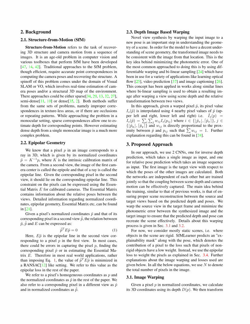
2.3. Depth Image Based WarpingNovel view synthesis by warping the input image to a

new pose is an important step in understanding the geome-try of a scene. In order for the model to have a decent under-standing of scene geometry, the transformed image needs tobe consistent with the image from that location. This is thekey idea behind minimizing the photometric error. One ofthe most common approached to doing this is by using dif-ferentiable warping and bi-linear sampling [24] which havebeen in use for a variety of applications like learning opticalflow [25], video prediction [37] and image captioning [26].This concept has been applied in works along similar lineswhere bi-linear sampling is used to obtain a resulting im-age after warping a view using scene depth and the relativetransformation between two views.

In this approach, given a warped pixel p, its pixel valueIs(p) is interpolated using 4 nearby pixel values of p (up-per left and right, lower left and right) i.e. Is(p) =Is(p) =

∑i

∑j wijIs(pij) where i ∈ {bpxc, dpxe}, j ∈

{bpyc, dpye} and wij is directly proportional to the prox-imity between p and pij such that

∑wij = 1. Further

explanation regarding this can be found in [24].

3. Proposed ApproachIn our approach, we use 2 CNNs, one for inverse depth

prediction, which takes a single image as input, and onefor relative pose prediction which takes an image sequenceas input. The first image is the target view with respect towhich the poses of the other images are calculated. Boththe networks are independent of each other but are trainedjointly so that the coupling between scene depth and cameramotion can be effectively captured. The main idea behindthe training, similar to that of previous works, is that of en-suring proper scene reconstruction between the source andtarget views based on the predicted depth and poses. Wewarp the source view in the target frame and minimize thephotometric error between the synthesized image and thetarget image to ensure that the predicted depth and pose canrecreate the scene effectively. Details about this warpingprocess is given in Sec. 3.1 and 3.2.

For now, we consider mostly static scenes, i.e. whereobjects in the scene are rigid. SfMLearner predicts an ”ex-plainability mask” along with the pose, which denotes thecontribution of a pixel to the loss such that pixels of non-rigid objects have a low weight. Instead, we use the epipolarloss to weight the pixels as explained in Sec. 3.4. Furtherexplanations about the image warping and losses used aregiven below. In all the below equations, we useN to denotethe total number of pixels in the image.

3.1. Image Warping

Given a pixel p in normalized coordinates, we calculateits 3D coordinates using its depth D(p). We then transform

Figure 1. Overview of the training procedure. The Depth CNN predicts the inverse depth for a target view. The Pose CNN predicts therelative poses of the source views from the target. The source views are warped into the target frame using the relative poses and the scenedepth and the photometric errors between multiple source-target pairs are minimized. These are weighted by the per-pixel epipolar losscalculated using the Essential Matrix obtained from the Five-Point Algorithm [36].

it into the source frame using the relative pose and projectit onto the source image’s plane.

p = K(Rt→sD(p)K−1p+ tt→s) (2)

where K is the camera calibration matrix, D(p) is thedepth of pixel p,Rt→s and tt→s are the rotation and transla-tion respectively from the target frame to the source frame.The homogeneous coordinates of p are continuous while werequire integer values. Thus, we interpolate the values fromnearby pixels, using bi-linear sampling, proposed by [24],as explained in Sec. 2.3.

3.2. Novel View Synthesis

We use novel view synthesis using depth image basedwarping as the main supervisory signal for our networks.Given the per-pixel depth and the relative poses betweenimages, we can synthesize the image of the scene from anovel viewpoint. We minimize the photometric error be-tween this synthesized image and the actual image from thegiven viewpoint. If the pose and depth are correctly pre-dicted, then the given pixel should be projected to its corre-sponding pixel in the image from the given viewpoint.

Given a target view It and N source views Is, we mini-mize the photometric error between the target view and thesource view warped into the target’s frame, denoted by Is.Mathematically, this can be described by Eq. 3

Lwarp =1

N

∑s

∑p

|It(p)− Is(p)| (3)

3.3. Spatial Smoothing

In order to tackle the issues of learning wrong depth val-ues for texture-less regions, we try to ensure that the depthprediction is derived from spatially similar areas. One morething to note is that depth discontinuities usually occur atobject boundaries. We minimize L1 norm of the spatialgradients of the inverse depth ∂d, weighted by the imagegradient ∂I . This is to account for sudden changes in depthdue to crossing of object boundaries and ensure a smoothchange in the depth values. This is similar to [18].

Lsmooth =1

N

∑p

(|∂xd(p)|e−|∂xI(p)|+|∂yd(p)|e−|∂yI(p)|)

(4)

3.4. Epipolar Constraints

The problem with simply minimizing the photometricerror is that it doesn’t take ambiguous pixels into consid-eration, such as those belonging to non-rigid objects, thosewhich are occluded etc. Thus, we need to weight pixels ap-propriately based on whether they’re properly projected ornot. One way of ensuring correct projection is by checkingif the corresponding pixel p lies on its epipolar line or not,according to Eq. 1.

We impose epipolar constraints using the Essential Ma-trix obtained from Nister’s Five Point Algorithm [36]. Thishelps ensure that the warped pixels to lie on their corre-sponding epipolar line. This epipolar loss ˆpTEp is usedto weight the above losses, where E is the Essential Ma-trix obtained using the Five Point Algorithm by computing

matches between features extracted using SiftGPU [46].After weighting, the new photometric loss now becomes

Lwarp =1

N

∑s

∑p

|It(p)− Is(p)|e|ˆpTEp| (5)

The reason behind this is that we wish to ensure properprojection of a pixel, rather than ensure just a low photo-metric error. If a pixel is projected correctly based on thepredicted depth and pose, its epipolar loss would be low.However, for a non-rigid object, even if the pixel is warpedcorrectly, with the pose and depth, the photometric errorwould be high. A high photometric error can also arisedue to incorrect warping. Therefore, to ensure that correctlywarped pixels aren’t penalized for belonging to moving ob-jects, we weight them with their epipolar distance, therebygiving their photmetric loss a lower weight than those thatare wrongly warped.

If the epipolar loss is high, it implies that the projection iswrong, giving a high weight to the photometric loss, therebyincreasing its overall penalty. This also helps in mitigatingthe problem of a pixel getting projected to a region of simi-lar intensity by constraining it to lie along the epipolar line.

3.5. Final Loss

Our final loss function is a weighted combination of theabove loss functions summed over multiple image scales.

Lfinal =∑l

(Llwarp + λsmoothL

lsmooth) (6)

where l iterates over the different scale values andλsmooth is the coefficient giving the relative weight for thesmoothness loss. Note that we don’t minimize the epipo-lar loss but use it for weighting the other losses. This waythe network tries to implicitly minimize the projection error(the epipolar loss) as it would lead to a reduction in the overall loss. Along with this it also minimizes the result of theprojection as well (photometric loss).

4. Implementation Details4.1. Neural Network Design

The Depth network is inspired from DispNet[33]. Ithas a design of a convolutional-deconvolutional encoder-decoder network with skip connections from previous lay-ers. The input is a single RGB image. We perform predic-tion at 4 different scales. We normalize the inverse-depthprediction to have unit mean, similar to what is done in thekey frames of LSD-SLAM [11] and in [45].

We modify the pose network proposed by [52] by remov-ing their ”explainability mask” layers thereby using lesserparameters yet giving better performance. The target viewand the source views are concatenated along the colourchannel giving rise to an input layer of size H ×W × 3N

where N is the number of input views. The network pre-dicts 6 DoF poses for each of theN−1 source views relativeto the target image.

We use batch normalization[23] for all the non-outputlayers. Details of network implementations are given in theappendix in Fig. A1.

4.2. Training

We implement the system using Tensorflow [1]. We useAdam [28] with β1 = 0.9, β2 = 0.999, a learning rate of0.0002 and a mini-batch of size 4 in our training. We setλsmooth = 0.2/2l where l is the scale, ranging from 0 -3. For training, we use the KITTI dataset[16] with the splitprovided by [9], which has about 40K images in total. Weexclude the static scenes (acceleration less than a limit) andthe test images from our training set. We use 3 views asthe input to the pose network during the training phase withthe middle image as our target image and the previous &succeeding images as the source images.

5. Results5.1. KITTI Depth Estimation Results

We evaluate our performance on the 697 images used by[9]. We show our results in Table 1. Our method’s per-formance exceeds that of SfMLearner and Yang et al.[50],both of which are monocular methods. We also beat meth-ods which use depth supervision [9, 30] and calibratedstereo supervision[15]. However, we fall short of Godardet al.[18], who also use stereo supervision and incorporateleft-right consistency, making their approach more robust.

In monocular methods, we fall short of GeoNet[51] andDDVO[45]. GeoNet[51] uses a separate encoder decodernetwork to predict optical flow from rigid flow, whichlargely increases the no. of parameters. DDVO[45], usesexpensive non-linear optimizations on top of the networkoutputs in each iteration, which is computationally inten-sive.

Our depth estimates deviate just marginally compared toLEGO[49]and Mahjourian et al.[31]. However, the com-plexity of our method is much lesser than LEGO[49], whichincorporates many complex losses (depth-normal consis-tency, surface normal consistency, surface depth consis-tency) and uses a much larger no. of parameters as theypredict edges as well. Mahjourian et al.[31] minimize theIterative Point Cloud (ICP) [3, 5, 38] alignment error be-tween predicted pointclouds, which is an expensive oper-ation, while ours uses just simple, standard epipolar con-straints. This shows that our method being simple, effec-tive and motivated by geometric association between multi-ple views produces comparable results with methods usingcomplex costs and more no. of parameters.

As shown in Fig. 2, our method performs better where

Image Ground truth SfMLearner Proposed Method

Figure 2. Results of depth estimation compared with SfMLearner. The ground truth is interpolated from sparse measurements. Some oftheir main failure cases are highlighted in the last 3 rows, such as large open spaces, texture-less regions, and when objects are present rightin front of the camera. As it can be seen in the last 3 rows, our method performs significantly better, providing more meaningful depthestimates even in such scenarios. (Pictures best viewed in color.)

SfMLearner fails, such as texture-less scenes and open re-gions. This shows the effectiveness of using epipolar geom-etry, rather training an extra parameter per-pixel to handleocclusions and non-rigidity. We also provide sharper out-puts which is a direct result of using an edge-aware smooth-ness that helps capture the shape of objects in a better man-ner. We scale our depth predictions to match the groundtruth depth’s median. Further details about the depth evalu-ation metrics can be found in [9].

5.2. Pose Estimation Results

We use sequences 00-10 of the KITTI Visual Odome-try Benchmark[17], which have the associated ground truth.We use the same model used for depth evaluation to re-port our pose estimation results (and of other SOTA meth-ods as well), rather than training a separate model with 5

views (as done by most works). We do so as we believethe same training scheme should suffice to efficiently learndepth and motion, rather than having different sets of exper-iments for each. We show the Avg. Trajectory Error (ATE)and Avg. Translational Direction Error (ATDE) averagedover 3 frame intervals in Table 2. Before ATE comparison,the scale is corrected to align it with the ground truth. SinceATDE compares only directions, we don’t correct the scale.

We perform better on all runs compared to the Five pt.alg. in terms of the ATDE. This is a result of having addi-tional feedback from image warping while the Five pt. alg.uses only sparse point correspondences.

We perform better than SfMLearner1 on an avg. show-ing that epipolar constraints help get better estimates. Weperform comparably (difference at scale of 10−2m) to

1using the model at github.com/tinghuiz/SfMLearner

Method Supervision Error Metric (lower is better) Accuracy Metric (higher is better)Abs. Rel. Sq. Rel. RMSE RMSE log δ < 1.25 δ < 1.252 δ < 1.253

Train set mean – 0.403 5.53 8.709 0.403 0.593 0.776 0.878Eigen et al. [9] Coarse Depth 0.214 1.605 6.563 0.292 0.673 0.884 0.957Eigen et al. [9] Fine Depth 0.203 1.548 6.307 0.282 0.702 0.89 0.958

Liu et al. [30] Depth 0.202 1.614 6.523 0.275 0.678 0.895 0.965Godard et al.[18] Stereo 0.148 1.344 5.927 0.247 0.803 0.922 0.964

DDVO[45] Mono 0.151 1.257 5.583 0.228 0.810 0.936 0.974Yang et al.[50] Mono 0.182 1.481 6.501 0.267 0.725 0.906 0.963

Geonet[51] (ResNet) Mono 0.155 1.296 5.857 0.233 0.793 0.931 0.973Geonet[51] (updated from github) Mono 0.149 1.060 5.567 0.226 0.796 0.935 0.975

Mahjourian et al.[31] Mono 0.163 1.240 6.220 0.250 0.762 0.916 0.968LEGO [49] Mono 0.162 1.352 6.276 0.252 0.783 0.921 0.969

SfMLearner (w/o explainability) Mono 0.221 2.226 7.527 0.294 0.676 0.885 0.954SfMLearner Mono 0.208 1.768 6.856 0.283 0.678 0.885 0.957

SfMLearner (updated from github) Mono 0.183 1.595 6.709 0.270 0.734 0.902 0.959Ours Mono 0.175 1.396 5.986 0.255 0.756 0.917 0.967

Garg et al. [15] Stereo 0.169 1.08 5.104 0.273 0.740 0.904 0.962GeoNet[51] (ResNet) Mono 0.147 0.936 4.348 0.218 0.810 0.941 0.977Mahjourian et al.[31] Mono 0.155 0.927 4.549 0.231 0.781 0.931 0.975

SfMLearner (w/o explainability) Mono 0.208 1.551 5.452 0.273 0.695 0.900 0.964SfMLearner Mono 0.201 1.391 5.181 0.264 0.696 0.900 0.966

Ours Mono 0.168 1.105 4.624 0.241 0.773 0.927 0.972

Table 1. Single View Depth results using the split of [9]. Garg et al.[15] cap their depth at 50m which we show in the bottom part of thetable. The dashed line separates methods that use some form of supervision from purely monocular methods. δ is the ratio between thescaled predicted depth and the ground truth. Further details about the error and accuracy metrics can be found in [9]. Baseline numberstaken from [45, 50, 51, 31, 48].

Seq Avg. Trajectory Error Avg. Translational Direction ErrorSfMLearner GeoNet[51] LEGO[49] Mahjourian et al.[31] Ours Five Pt. Alg. Ours

00 0.5099±0.2471 0.4975±0.1791 0.4973±0.1893 0.4955±0.1727 0.4969±0.1775 0.0084±0.0821 0.0040±0.015601 1.2290±0.2518 1.1474±0.2177 1.1665±0.2261 1.1365±0.2136 1.1433±0.2156 0.0061±0.0807 0.0032±0.007402 0.6330±0.2328 0.6492±0.1796 0.6476±0.1858 0.6552±0.1809 0.6509±0.1797 0.0035±0.0509 0.0021±0.002603 0.3767±0.1527 0.3593±0.1243 0.3610±0.1294 0.3587±0.1237 0.3592±0.1239 0.0142±0.1611 0.0027±0.004204 0.4869±0.0537 0.6357±0.0604 0.6062±0.0597 0.6603±0.0625 0.6439±0.0604 0.0182±0.2131 0.0002±0.001305 0.5013±0.2564 0.4918±0.1996 0.4935±0.2060 0.4925±0.1943 0.4920±0.1984 0.0130±0.0945 0.0043±0.004706 0.5027±0.2605 0.5394±0.1624 0.5308±0.1796 0.5434±0.1541 0.5392±0.1616 0.0130±0.1591 0.0080±0.069907 0.4337±0.3254 0.4001±0.2412 0.4115±0.2513 0.3979±0.2313 0.3993±0.2401 0.0508±0.2453 0.0112±0.044508 0.4824±0.2396 0.4714±0.1811 0.4714±0.1910 0.4714±0.1794 0.4715±0.1807 0.0091±0.0646 0.0037±0.005709 0.6652±0.2863 0.6292±0.2039 0.6310±0.2153 0.6234±0.1944 0.6288±0.2026 0.0204±0.1722 0.0072±0.021310 0.4672±0.2398 0.4165±0.1825 0.4269±0.1834 0.4149±0.1754 0.4163±0.1820 0.0200±0.1241 0.0036±0.0084

Table 2. Average Trajectory Error (ATE) compared with SfMLearner and Mahjourian et al.[31] and LEGO [49] & Average TranslationalDirection Error (ATDE) compared with the Five Point algorithm averaged over 3 frame snippets on the KITTI Visual Odometry Dataset[17]. ATE is shown in meters and ATDE, in radians. All values are reported as mean ± std. dev.

GeoNet[51]2, Mahjourian et al[31]3 and LEGO[49], all ofwhom use computationally expensive losses and a larger no.of parameters, compared to our method which is much sim-pler, yet effective and uses lesser no. of parameters. Theauthors of LEGO[49] don’t provide a pre-trained model,hence the results shown are after running their model4 for24 epochs.

5.3. Epipolar Loss for discounting motions

We demonstrate the efficacy of using the epipolar lossfor discounting ambiguous pixels. As mentioned in the last

2using scale normalized model at github.com/yzcjtr/GeoNet3using model at sites.google.com/view/vid2depth4github.com/zhenheny/LEGO

paragraph of Sec. 3.4, the epipolar loss is useful to give arelatively lower weight to pixels that are properly warped,but belong to non-rigid objects. As seen in Fig. 3, the epipo-lar masks capture the moving objects (cyclists and cars)in the scene effectively, hence they can be used instead oflearning motion masks.

5.4. Cityscapes Depth EstimationWe compare our model with SfMLearner (both trained

on KITTI) on the Cityscapes dataset [7, 6], which is a sim-ilar urban outdoor driving dataset. These images are pre-viously unseen to the networks. As it can be seen in Fig.4, our model shows better depth outputs on unseen data,showing better generalization capabilities.

Figure 3. Epipolar mask visualization. The top is the target image, middle is the source, and bottom is a heatmap of the epipolar weights.

Image SfMLearner Proposed Method

Figure 4. Results of depth estimation compared with SfMLearner on the Cityscapes dataset. Note that the models that were trained onlyon the KITTI dataset are tested directly on the Cityscapes dataset without any fine-tuning. These images are previously unseen by thenetworks. (Pictures best viewed in colour.)

5.5. Make3D Depth Estimation

We compare our model trained on KITTI with SfM-Learner, on Make3D [41], a collection of still outdoor non-street images, unlike KITTI or Cityscapes. We center-cropthe images before predicting depth. Fig. 5 shows that our

method produces better depth outputs on previously unseenimages that are quite different from training images show-ing that it effectively generalizes to unseen data.

Image Ground Truth SfMLearner Ours

Figure 5. Results of our model trained on KITTI tested with Make3D

Method Error Metric (lower is better) Accuracy Metric (higher is better)Abs. Rel. Sq. Rel. RMSE RMSE log δ < 1.25 δ < 1.252 δ < 1.253

SfMLearner (w/o explainability) 0.221 2.226 7.527 0.294 0.676 0.885 0.954Ours (only epi) 0.217 1.639 6.746 0.297 0.651 0.875 0.954

Ours (only depth-norm) 0.187 1.726 6.530 0.272 0.727 0.904 0.960Ours (final) 0.175 1.396 5.986 0.255 0.756 0.917 0.967

Table 3. Ablative study on the effect of different losses in depth estimation. We show our results using the split of [9] while removing theproposed losses. We compare our method with SfMLearner (w/o explainability) which is essentially similar to stripping our method of theproposed losses and using a different smoothness loss.

6. Ablation Study

We perform an ablation study on the depth estimationby considering variants of our proposed approach. Thebaseline for comparison is SfMLearner w/o explainability,which is equivalent to removing our additions and having asimpler 2nd order smoothness loss. We first see the effectof adding just the epipolar constraints, denoted by ”Ours(only epi)”. We then see how adding just the inverse-depthnormalization ”Ours (only depth-norm)” affects the perfor-mance. Finally we combine all the proposed additions giv-ing rise to our final loss funtion, denoted by ”Ours (final)”.

The results of the study can be seen in Table 3. Allour variants perform significantly better than SfMLearnershowing that our method has a positive effect on the learn-ing. Just adding the epipolar constraints improves the re-sults over SfMLearner. The inverse-depth normalizationgives a significant improvement as it constrains the depthto lie in a suitable range, which would otherwise cause theinverse-depth to decrease over iterations, leading to a de-crease in the smoothness loss, as explained in [45]. Finally,combining them all, produces better results than either ofthe additions individually, showing the effectiveness of ourproposed method.

7. Conclusion and Future Work

We improve upon a previous unsupervised method forlearning monocular visual odometry and single view depthestimation while using lesser number of trainable parame-ters in a simplistic manner. Our method is able to predictsharper and more accurate depths as well as better pose es-timates. Other than just KITTI, we also show better perfor-mance on Cityscapes and Make3D as well, using the modeltrained with just KITTI. This shows that our method gener-alizes well to unseen data. With just a simple addition, weare able to get performance similar to state-of-the-art meth-ods that use complex losses.

The current method however only performs pixel levelinferences. A higher scene level understanding can be ob-tained by integrating semantics to get better correlation be-tween objects in the scene and depth & ego-motion esti-mates, similar to semantic motion segmentation [19, 20].

Architectural changes could be leveraged by performingmulti-view depth prediction to learn how the depth variesover multiple frames or having a single network for bothpose and depth to help capture the complex relation betweencamera motion and scene depth.

References[1] M. Abadi, P. Barham, J. Chen, Z. Chen, A. Davis, J. Dean,

M. Devin, S. Ghemawat, G. Irving, M. Isard, et al. Tensor-flow: A system for large-scale machine learning. In Operat-ing Systems Design and Implementation (OSDI), 2016. 4

[2] H. Alismail, B. Browning, and S. Lucey. Enhancing directcamera tracking with dense feature descriptors. In ACCV,2016. 2

[3] P. J. Besl and N. D. McKay. A method for registration of 3-dshapes. IEEE Transactions on Pattern Analysis and MachineIntelligence, 1992. 4

[4] A. Byravan and D. Fox. Se3-nets: Learning rigid body mo-tion using deep neural networks. In ICRA, 2017. 1

[5] Y. Chen and G. Medioni. Object modeling by registration ofmultiple range images. In ICRA, 1991. 4

[6] M. Cordts, M. Omran, S. Ramos, T. Rehfeld, M. Enzweiler,R. Benenson, U. Franke, S. Roth, and B. Schiele. Thecityscapes dataset for semantic urban scene understanding.In CVPR, 2016. 6

[7] M. Cordts, M. Omran, S. Ramos, T. Scharwachter, M. En-zweiler, R. Benenson, U. Franke, S. Roth, and B. Schiele.The cityscapes dataset. In CVPR Workshop on The Future ofDatasets in Vision, 2015. 6

[8] V. Duggal, K. Bipin, U. Shah, and K. M. Krishna. Hierar-chical structured learning for indoor autonomous navigationof quadcopter. In Indian Conference on Computer Vision,Graphics and Image Processing (ICVGIP), 2016. 1

[9] D. Eigen, C. Puhrsch, and R. Fergus. Depth map predictionfrom a single image using a multi-scale deep network. InNIPS, 2014. 1, 4, 5, 6, 8

[10] J. Engel, V. Koltun, and D. Cremers. Direct sparse odometry.TPAMI, 2018. 2

[11] J. Engel, T. Schops, and D. Cremers. Lsd-slam: Large-scaledirect monocular slam. In ECCV, 2014. 2, 4

[12] M. A. Fischler and R. C. Bolles. Random sample consen-sus: a paradigm for model fitting with applications to imageanalysis and automated cartography. Communications of theACM, 1981. 2

[13] C. Forster, M. Pizzoli, and D. Scaramuzza. Svo: Fast semi-direct monocular visual odometry. In ICRA, 2014. 2

[14] Y. Furukawa, B. Curless, S. M. Seitz, and R. Szeliski. To-wards internet-scale multi-view stereo. In CVPR, 2010. 2

[15] R. Garg, V. K. BG, G. Carneiro, and I. Reid. Unsupervisedcnn for single view depth estimation: Geometry to the res-cue. In ECCV, 2016. 1, 4, 6

[16] A. Geiger, P. Lenz, C. Stiller, and R. Urtasun. Vision meetsrobotics: The kitti dataset. IJRR, 2013. 4

[17] A. Geiger, P. Lenz, and R. Urtasun. Are we ready for au-tonomous driving? the kitti vision benchmark suite. InCVPR, 2012. 5, 6

[18] C. Godard, O. Mac Aodha, and G. J. Brostow. Unsupervisedmonocular depth estimation with left-right consistency. InCVPR, 2017. 1, 3, 4, 6

[19] N. Haque, N. D. Reddy, and K. M. Krishna. Joint seman-tic and motion segmentation for dynamic scenes using deepconvolutional networks. In International Joint Conference

on Computer Vision, Imaging and Computer Graphics The-ory and Applications (VISAPP), 2017. 8

[20] N. Haque, N. D. Reddy, and M. Krishna. Temporal seman-tic motion segmentation using spatio temporal optimization.In International Workshop on Energy Minimization Methodsin Computer Vision and Pattern Recognition (EMMCVPR),2017. 8

[21] R. Hartley and A. Zisserman. Multiple view geometry incomputer vision. Cambridge university press, 2003. 2

[22] D. Hoiem, A. A. Efros, and M. Hebert. Automatic photopop-up. In ACM Transactions on Graphics (TOG), 2005. 1

[23] S. Ioffe and C. Szegedy. Batch normalization: Acceleratingdeep network training by reducing internal covariate shift.ICML, 2015. 4

[24] M. Jaderberg, K. Simonyan, A. Zisserman, et al. Spatialtransformer networks. In NIPS, 2015. 2, 3

[25] J. Y. Jason, A. W. Harley, and K. G. Derpanis. Back to ba-sics: Unsupervised learning of optical flow via brightnessconstancy and motion smoothness. In ECCV, 2016. 2

[26] J. Johnson, A. Karpathy, and L. Fei-Fei. Densecap: Fullyconvolutional localization networks for dense captioning. InCVPR, 2016. 2

[27] J. Jose Tarrio and S. Pedre. Realtime edge-based visualodometry for a monocular camera. In ICCV, 2015. 2

[28] D. P. Kingma and J. Ba. Adam: A method for stochasticoptimization. In ICLR, 2015. 4

[29] G. Klein and D. Murray. Parallel tracking and mapping forsmall ar workspaces. In International Symposium on Mixedand Augmented Reality (ISMAR), 2007. 2

[30] F. Liu, C. Shen, G. Lin, and I. Reid. Learning depth from sin-gle monocular images using deep convolutional neural fields.TPAMI, 2016. 4, 6

[31] R. Mahjourian, M. Wicke, and A. Angelova. Unsupervisedlearning of depth and ego-motion from monocular video us-ing 3d geometric constraints. In CVPR, 2018. 4, 6

[32] S. Maity, A. Saha, B. Bhowmick, C. Park, S. Kim,P. Moghadam, C. Fookes, S. Sridharan, I. Eichhardt, L. Ha-jder, et al. Edge slam: Edge points based monocular visualslam. In ICCV Workshops (ICCVW), 2017. 2

[33] N. Mayer, E. Ilg, P. Hausser, P. Fischer, D. Cremers,A. Dosovitskiy, and T. Brox. A large dataset to train convo-lutional networks for disparity, optical flow, and scene flowestimation. In CVPR, 2016. 4

[34] R. Mur-Artal, J. M. M. Montiel, and J. D. Tardos. Orb-slam:a versatile and accurate monocular slam system. TRO, 2015.2

[35] R. A. Newcombe, S. J. Lovegrove, and A. J. Davison. Dtam:Dense tracking and mapping in real-time. In ICCV, 2011. 2

[36] D. Nister. An efficient solution to the five-point relative poseproblem. TPAMI, 2004. 1, 3

[37] V. Patraucean, A. Handa, and R. Cipolla. Spatio-temporalvideo autoencoder with differentiable memory. arXivpreprint arXiv:1511.06309, 2015. 2

[38] S. Rusinkiewicz and M. Levoy. Efficient variants of the icpalgorithm. In IEEE International Conference on 3-D DigitalImaging and Modeling, 2001. 4

[39] A. Saxena, H. Pandya, G. Kumar, A. Gaud, and K. M. Kr-ishna. Exploring convolutional networks for end-to-end vi-sual servoing. In ICRA, 2017. 1

[40] A. Saxena, M. Sun, and A. Y. Ng. Learning 3-d scene struc-ture from a single still image. In ICCV, 2007. 1

[41] A. Saxena, M. Sun, and A. Y. Ng. Make3d: Learning 3dscene structure from a single still image. IEEE Transactionson Pattern Analysis and Machine Intelligence, 2009. 7

[42] P. Sturm and B. Triggs. A factorization based algorithmfor multi-image projective structure and motion. In ECCV,1996. 2

[43] B. Ummenhofer, H. Zhou, J. Uhrig, N. Mayer, E. Ilg,A. Dosovitskiy, and T. Brox. Demon: Depth and motionnetwork for learning monocular stereo. In CVPR, 2017. 1

[44] S. Vijayanarasimhan, S. Ricco, C. Schmid, R. Sukthankar,and K. Fragkiadaki. Sfm-net: Learning of structure and mo-tion from video. arXiv:1704.07804, 2017. 1

[45] C. Wang, J. M. Buenaposada, R. Zhu, and S. Lucey. Learn-ing depth from monocular videos using direct methods. InCVPR, 2018. 4, 6, 8

[46] C. Wu. Siftgpu: A gpu implementation of sift. 2007. 4[47] C. Wu. Towards linear-time incremental structure from mo-

tion. In 3DV, 2013. 2[48] Z. Yang, P. Wang, Y. Wang, W. Xu, and R. Nevatia. Every

pixel counts: Unsupervised geometry learning with holistic3d motion understanding. arXiv preprint arXiv:1806.10556,2018. 6

[49] Z. Yang, P. Wang, Y. Wang, W. Xu, and R. Nevatia. Lego:Learning edge with geometry all at once by watching videos.In CVPR, 2018. 4, 6

[50] Z. Yang, P. Wang, W. Xu, L. Zhao, and R. Nevatia. Unsu-pervised learning of geometry from videos with edge-awaredepth-normal consistency. In AAAI, 2018. 1, 4, 6

[51] Z. Yin and J. Shi. Geonet: Unsupervised learning of densedepth, optical flow and camera pose. In CVPR, 2018. 1, 4, 6

[52] T. Zhou, M. Brown, N. Snavely, and D. G. Lowe. Unsu-pervised learning of depth and ego-motion from video. InCVPR, 2017. 1, 4

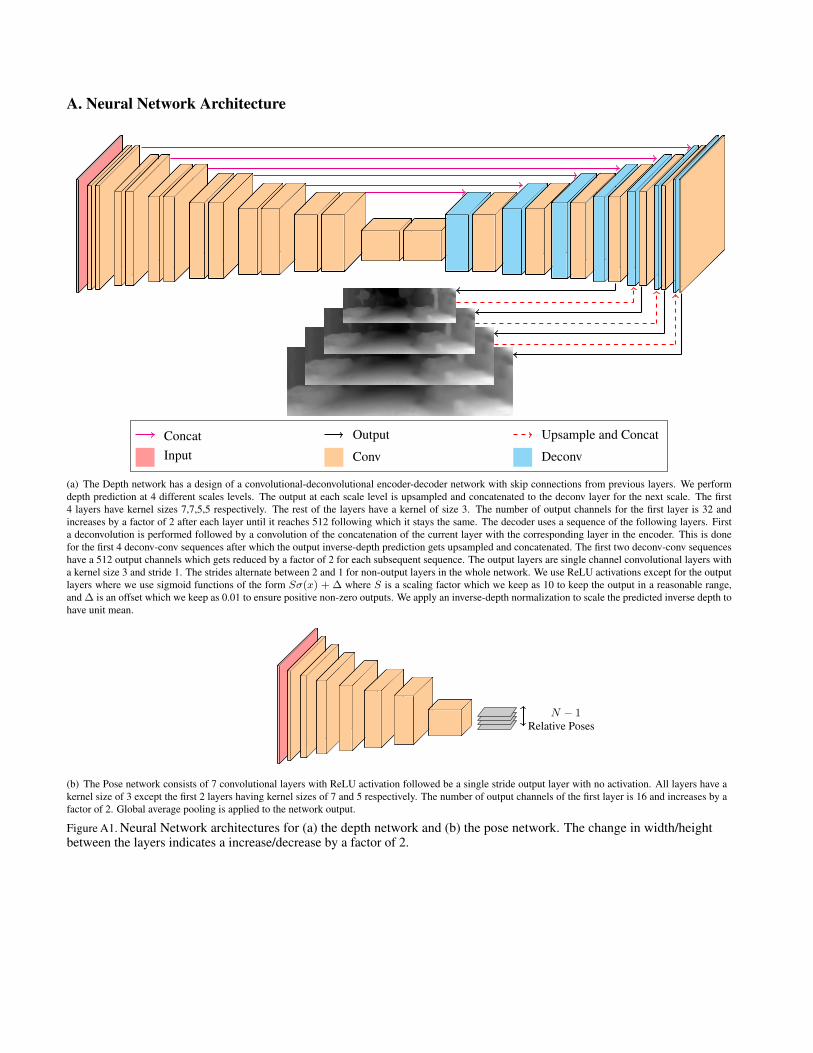
A. Neural Network Architecture

Concat Output Upsample and Concat

Input Conv Deconv

(a) The Depth network has a design of a convolutional-deconvolutional encoder-decoder network with skip connections from previous layers. We performdepth prediction at 4 different scales levels. The output at each scale level is upsampled and concatenated to the deconv layer for the next scale. The first4 layers have kernel sizes 7,7,5,5 respectively. The rest of the layers have a kernel of size 3. The number of output channels for the first layer is 32 andincreases by a factor of 2 after each layer until it reaches 512 following which it stays the same. The decoder uses a sequence of the following layers. Firsta deconvolution is performed followed by a convolution of the concatenation of the current layer with the corresponding layer in the encoder. This is donefor the first 4 deconv-conv sequences after which the output inverse-depth prediction gets upsampled and concatenated. The first two deconv-conv sequenceshave a 512 output channels which gets reduced by a factor of 2 for each subsequent sequence. The output layers are single channel convolutional layers witha kernel size 3 and stride 1. The strides alternate between 2 and 1 for non-output layers in the whole network. We use ReLU activations except for the outputlayers where we use sigmoid functions of the form Sσ(x) + ∆ where S is a scaling factor which we keep as 10 to keep the output in a reasonable range,and ∆ is an offset which we keep as 0.01 to ensure positive non-zero outputs. We apply an inverse-depth normalization to scale the predicted inverse depth tohave unit mean.

N − 1Relative Poses

(b) The Pose network consists of 7 convolutional layers with ReLU activation followed be a single stride output layer with no activation. All layers have akernel size of 3 except the first 2 layers having kernel sizes of 7 and 5 respectively. The number of output channels of the first layer is 16 and increases by afactor of 2. Global average pooling is applied to the network output.

Figure A1. Neural Network architectures for (a) the depth network and (b) the pose network. The change in width/heightbetween the layers indicates a increase/decrease by a factor of 2.