WP 13.2

16 October 2013

UNITED NATIONS STATISTICAL COMMISSION

and ECONOMIC COMMISSION FOR EUROPE

STATISTICAL OFFICE OF THE

EUROPEAN UNION (EUROSTAT)

Joint Eurostat/UNECE Work Session on Demographic Projections

organised in cooperation with Istat

(29-31 October 2013, Rome, Italy)

Item 13 – Bayesian approaches

Bayesian Probabilistic Population Projections: Do It Yourself

Hana Sevcikova, University of Washington

Adrian E. Raftery, University of Washington and University College Dublin

Patrick Gerland, United Nations

Bayesian Probabilistic Population Projections:

Do It Yourself

Hana Sevcıkova, University of WashingtonAdrian E. Raftery, University of Washington and University College Dublin

Patrick Gerland, United Nations

September 30, 2013

Abstract

A Bayesian approach for probabilistic population projections has recently been used by the UnitedNation Population Division in the preparation of the 2012 revision of the World Population Prospects.The methods have been implemented in publicly available open-source software as a collection ofR packages. In this paper, we demonstrate how to easily reproduce such population projections,including probabilistic projections of total fertility rate and life expectancy. The packages allow anyanalysts to generate variations of the UN projections, to use their own data, to impute missing dataand to produce aggregated projections for regions consisting of multiple countries. Using a flexibleexpression language, probabilistic results can be summarized and visualized in graphs, maps, orpopulation pyramids. The software can be conveniently controlled from a graphical user interface.

1 Introduction

A systematic framework for producing probabilistic population projections for all countries, both devel-oped and developing, has recently been proposed by Raftery et al. (2012). It consists of probabilisticallyprojecting total fertility rate and life expectancy using Bayesian hierarchical models (Alkema et al.,2011; Raftery, Chunn, Gerland & Sevcıkova, 2013), converting the results to age-specific rates, andprojecting the population forward using the cohort-component method applied to each trajectory sim-ulated from their predictive distributions. The median projection from these rates has been used as theUN’s official medium projection for all countries in the 2012 revision of the World Population Prospects,or WPP (United Nations, 2013).

Here we describe a suite of software packages developed to allow users beyond the UN to implementthe methodology. These are four R packages: bayesTFR to project total fertility rate, bayesLife toproject life expectancy, bayesPop to project population, and a graphical user interface, bayesDem. Allare freely available. We also introduce a package for interactive visual exploration of various indicatorsderived from WPP data, called wppExplorer.

In this paper, we show how to reproduce such probabilistic population projections, including proba-bilistic projections of total fertility rate and life expectancy. The packages allow any analyst to generatevariations of the UN projections, to use their own data, to impute missing data or to apply the methodsto sub-national datasets. We also introduce a flexible expression language which allows probabilisticresults to be summarized and visualized in graphs, maps or population pyramids. The software can beconveniently controlled from a graphical user interface.

The paper is organized as follows. In Section 2 we review the basic methodology underlying the prob-abilistic projections. In Section 3, we describe the bayesTFR package for projecting the total fertility

1

rate. In Section 4, we outline the bayesLife package for projecting life expectancy. In Section 5, wedescribe the bayesPop package for population projection. This covers methods for obtaining futurepopulation trajectories, for viewing the trajectories in various ways and for producing probabilisticpopulation pyramids. It also describes the expression language for projecting a wide range of derivedpopulation quantities. Finally, Section 6 discusses the graphical user interface bayesDem and wppEx-plorer.

2 Methodology

Almost all methods used for predicting population Pc,t in country c at time period t are based on thedemographic balancing equation

Pc,t = Pc,t−1 + Bc,t −Dc,t + Mc,t

where B denotes the number of births, D the number of deaths and M net migration. In mostapplications this equation is solved deterministically using the cohort component method (Whelpton,1928, 1936) which decomposes it into age- and sex-specific components.

The traditional UN methodology of population projections (United Nations, 1956, 1989) for future timeperiods t > 0 follows the cohort component method and for that purpose, it uses the following inputsfor each country:

• Sex- and age-specific population estimates at the initial time t = 0

• Projections of total fertility rate (TFR)

• Projections of fertility distribution over ages

• Projections of sex ratio at birth

• Projections of male and female life expectancy at birth (e0)

• Historical data on sex- and age-specific death rates (for t ≤ 0)

• Projections of sex- and age-specific net migration

In each future time period t, the projected TFR is converted to age-specific fertility rates using the fer-tility distribution over ages at t. Using the historical data on death rates, the projected life expectancyis converted to age-specific mortality rates using a variant of the Lee-Carter method (Lee & Carter,1992). Then the cohort component model is applied.

To communicate uncertainty in the context of this deterministic approach, until recently, the UN usedthree scenarios, the high, medium and low variants. Here, the medium variant is the main projection.The high and low variants have been generated by adding plus or minus half a child to the TFR,respectively, and applying the method above. Such approach suffers from not having a probabilisticbasis and can lead to inconsistencies (Lee & Tuljapurkar, 1994; National Research Council, 2000).

Recently approaches to probabilistic projections of two main input components were introduced, namelyTFR (Alkema et al., 2011) and life expectancy (Raftery, Chunn, Gerland & Sevcıkova, 2013). Rafteryet al. (2012) describes a methodology for combining these components into probabilistic populationprojections. The idea is to

1. simulate a large set of trajectories of future values of TFR,

2

2. simulate an equal number of trajectories of life expectancy,

3. convert each of the trajectories into a future trajectory of sex- and age-specific population quantity,using the current UN methodology as described above.

The resulting set of values is viewed as a sample from the predictive distribution of population projec-tions.

This process is fully supported by open-source packages implemented in R (Ihaka & Gentleman, 1996).The simulation of TFR trajectories (1.) is implemented in a package called bayesTFR (Sevcıkova et al.,2011). Life expectancy trajectories (2.) can be generated using the package bayesLife (Sevcıkova &Raftery, 2013b). Finally, population projections by age and sex (3.) can be obtained using the packagebayesPop (Sevcıkova & Raftery, 2013a). A graphical user interface (GUI) for the three packages isprovided by the R package bayesDem (Sevcıkova, 2013a). One can generate probabilistic projectionsof TFR and life expectancy, and combine those results into probabilistic population projections from asingle interface, see Figure 1.

bayesDem

Analyse and visualize MCMC results

Check convergence

Plot maps

bayesTFR

bayesPop

bayesLife

Project population

trajectories

Analyse and visualize projection trajectories

Analyse and visualize MCMC results

Check convergence

Plot maps

Analyse and visualize projection trajectories

Estimate TFR parameters

Project TFR trajectories

Estimate e0 parameters

Plot maps

wp

p2012

(UN

dat

aset

s)

Project female and male

e0 trajectories

Analyse projection trajectories

Plot trajectories and pyramids

Figure 1: Structure of packages supported by bayesDem. Boxes shown on the left-hand side (connectedby blue arrows) depict the main steps needed for generating probabilistic population projections. Boxeson the right-hand side show supporting functionality of the packages. The packages operate on UNdatasets included in the wpp2012 package.

In what follows, we assume that the reader is somewhat familiar with basic R syntax. Furthermore, inorder to reproduce the code examples in the text, R and the three packages, bayesTFR, bayesLife and

3

● ● ●● ●

●●

●●

●●

●

●● ●

● ●●

● ●●

●

●

●

●

●

● ●

●●

● ● ●

●

●

●

●●

● ● ●●

1800 1850 1900 1950 2000

1.5

2.0

2.5

3.0

3.5

4.0

4.5

Denmark

Time

TF

R

●●

● ●●

●

●

●

●

●

● ●

●●

● ● ●

●

●

●

●●

● ● ●● ●

●●

●●

●●

●

●● ●

●

● ● ●●

●

●

●

Pre−transition phase I (not modeled)Transition phase IIPost−transition phase III

fct (decreasing)

0

∆∆c1 ∆∆c2 ∆∆c3 ∆∆c4

0∆∆c4Uc=ΣΣ∆∆ci

dc

0.1dc

0.8dc

g((θθc,, fct))

Figure 2: Left panel: TFR time series for Denmark divided into three phases. Right panel: Hypotheticaldouble logistic decline function plotted agains TFR.

bayesPop should be installed. One can accomplish the package installation simply by calling

> install.packages("bayesPop", dependencies=TRUE)

from the R environment. This installs all three packages at once. To load them into the environment,type the command

> library(bayesPop)

When describing a function, only its main functionality will be mentioned, without going into greatdetail about its arguments. More information can be obtained from the functions’ help pages, using?function name.

3 Total Fertility Rate

The bayesTFR package (Sevcıkova et al., 2011) implements a methodology for probabilistic projectionof TFR as proposed by Alkema et al. (2011) and Raftery, Alkema & Gerland (2013).

The model is based on the observation that the evolution of the TFR includes three broad phases,referred to as Phase I, II and III: (I) a high-fertility pre-transition phase, (II) the fertility transition inwhich the TFR decreases from high fertility levels towards or below replacement level fertility, and (III)a low-fertility post-transition phase, which includes recovery from below-replacement fertility towardreplacement fertility and oscillations around replacement-level fertility. The left panel of Figure 2 showsan example of a TFR time series for Denmark divided into the three phases.

Phase II, the fertility transition phase, is modeled by a random walk with a nonconstant drift. Thedrift, or TFR decline, is a double logistic function with a country-specific set of parameters thatdefines the shape of the decline curve (see right panel of Figure 2). These parameters are estimatedusing a Bayesian hierarchical model in which the country-specific decline curves arise from a “world”distribution. Alkema et al. (2011) and Sevcıkova et al. (2011) describe this part of the model in moredetail.

4

Phase III, the post-transition phase is modeled as a first-order autoregressive model where the modelparameters are allowed to vary between countries, following a Bayesian hierarchical model (Raftery,Alkema & Gerland, 2013).

3.1 Simulating TFR Future Trajectories

This section explains how to generate TFR future trajectories using the bayesTFR package. Afterloading the package into the environment as shown in Section 2, choose a directory on which thepackage will operate:

> tfr.dir <- "/my/TFR/directory"

There are three main steps to obtain TFR projections, each of which translates into one function call:

1. Estimate the parameters of the Phase II model using Markov Chain Monte Carlo (MCMC):

> mc1 <- run.tfr.mcmc(output.dir=tfr.dir, iter="auto", wpp.year=2012,

start.year=1950, present.year=2010)

Note that such a call is set up to produce long MCMC chains, ideally passing convergence di-agnostics. Thus, its processing can take a very long time, possibly multiple days. Setting anoptional argument parallel=TRUE could significantly improve the run time as it processes allchains (three by default) in parallel. However, for a toy simulation, one can set the argumentiter to a small number, for example on the order of tens, but for somewhat realistic simulationiter should be on the order of ten thousands. The argument wpp.year determines which histor-ical data are being used; in this case it is a dataset from the R package wpp2012 (Sevcıkova et al.,2013). For some countries, that dataset goes back to year 1750 and the argument start.year

determines the first time period to be used, i.e. data prior to start.year are ignored. If ananalyst wishes to (possibly partly) replace the default UN dataset with his/her own data, anargument my.tfr.file can be used that points to a user-defined historical TFR dataset. Suchdataset must follow the same structure as the default UN dataset, which can be seen with thecommands data(tfr, package="wpp2012"); head(tfr). The package contains a template filefor this purpose, called “my tfr template.txt”, located in the package directory “inst/extdata”.

2. Estimate the parameters of the Phase III model by MCMC:

> mc2 <- run.tfr3.mcmc(sim.dir=tfr.dir, iter="auto")

The Phase III MCMCs will run substantially faster than step 1. Nevertheless again, iter shouldbe decreased for a toy simulation. Any time-specific arguments are inherited from the Phase IIsimulation. In the estimation, the historical TFR values from countries that reached Phase IIIbetween start.year and present.year are used. Again, the default historical dataset can beoverwritten with a user-specific one using the optional argument my.tfr.file.

3. Using the estimated parameters, generate future TFR trajectories:

> tfr.pred <- tfr.predict(sim.dir=tfr.dir, end.year=2100, use.diagnostics=TRUE)

The use.diagnostics argument should be set to TRUE only if iter="auto" was used in theestimation commands. In such a case, the MCMC burn-in and thin (or equivalently number

5

of trajectories) is automatically determined from existing diagnostics. If a toy simulation wasgenerated, these values should be provided explicitly, e.g. burnin=10, burnin3=10, nr.traj=100.This command produces a set of future TFR trajectories for each country included in the historicaldataset and stores it in the simulation directory. Any missing values prior to present.year (setin Step 1) are treated as projections and are imputed by the median of the posterior distribution.Note that only consecutive missing values at the end of the time series are allowed.

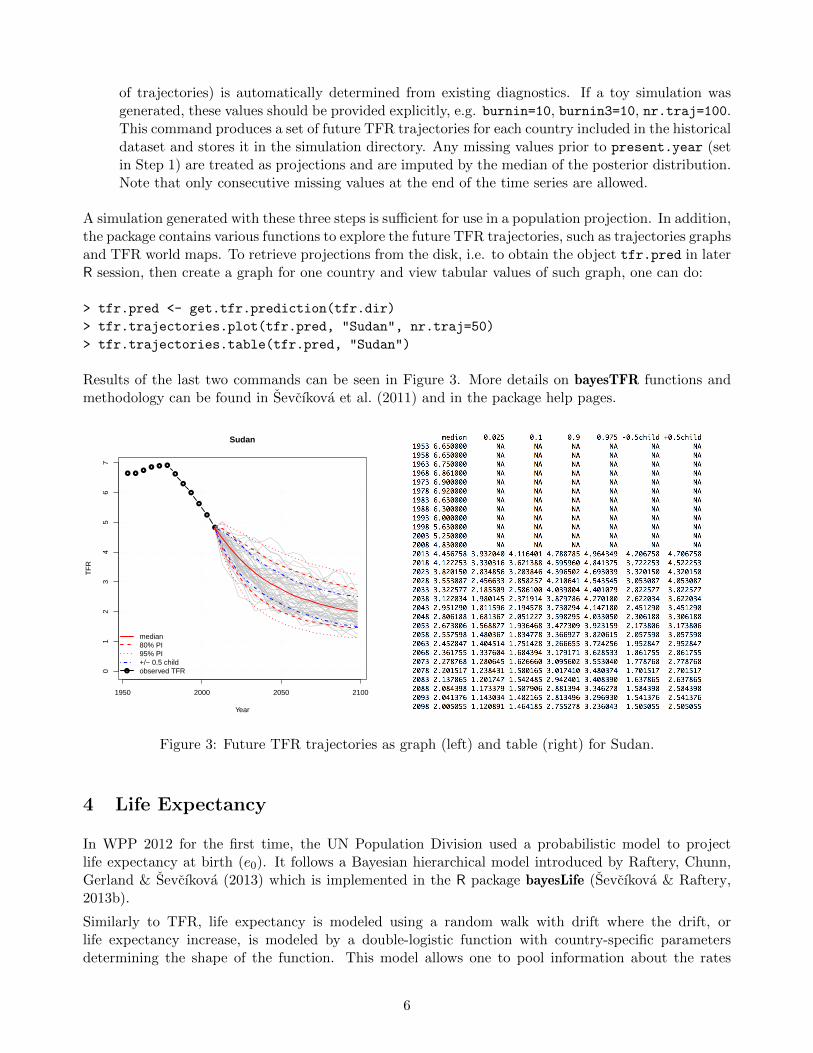
A simulation generated with these three steps is sufficient for use in a population projection. In addition,the package contains various functions to explore the future TFR trajectories, such as trajectories graphsand TFR world maps. To retrieve projections from the disk, i.e. to obtain the object tfr.pred in laterR session, then create a graph for one country and view tabular values of such graph, one can do:

> tfr.pred <- get.tfr.prediction(tfr.dir)

> tfr.trajectories.plot(tfr.pred, "Sudan", nr.traj=50)

> tfr.trajectories.table(tfr.pred, "Sudan")

Results of the last two commands can be seen in Figure 3. More details on bayesTFR functions andmethodology can be found in Sevcıkova et al. (2011) and in the package help pages.

1950 2000 2050 2100

01

23

45

67

Sudan

Year

TF

R

● ●●

● ● ●

●

●

●

●

●

●

●

median80% PI95% PI+/− 0.5 childobserved TFR

Figure 3: Future TFR trajectories as graph (left) and table (right) for Sudan.

4 Life Expectancy

In WPP 2012 for the first time, the UN Population Division used a probabilistic model to projectlife expectancy at birth (e0). It follows a Bayesian hierarchical model introduced by Raftery, Chunn,Gerland & Sevcıkova (2013) which is implemented in the R package bayesLife (Sevcıkova & Raftery,2013b).

Similarly to TFR, life expectancy is modeled using a random walk with drift where the drift, orlife expectancy increase, is modeled by a double-logistic function with country-specific parametersdetermining the shape of the function. This model allows one to pool information about the rates

6

of gains across countries by assuming that each set of country-specific double-logistic parameters israndomly sampled from a common (world) distribution.

The population projection methodology requires projections of female and male life expectancy simul-taneously. Generating them independently from the model of Raftery, Chunn, Gerland & Sevcıkova(2013) is unsatisfactory because there is generally a strong relationship between them, and ignoringthis can lead to future trajectories of female and male life expectancy that diverge unrealistically.

Lalic & Raftery (2012) proposed a method for joint projections of female and male life expectancy thatmodels the gap between them, the gap being defined as female e0 minus male e0. In such a model,projections of female life expectancy are generated by the Bayesian hierarchical model, and are thencombined with projections of the gap to produce projections of male life expectancy.

4.1 Simulating Future Trajectories of Life Expectancy

The implementation of the Bayesian hierarchical model in bayesLife closely follows the structure ofthe bayesTFR package. Many functions in one package have their analogues in the other, and theirnames differ only in the part called “tfr” versus “e0”. As for TFR, we first set a directory for the e0simulation:

> e0.dir <- "/my/e0/directory"

Obtaining e0 projections involves two steps:

1. Estimate parameters for female e0 via MCMC:

> mc <- run.e0.mcmc(output.dir=e0.dir, sex="Female", iter="auto", wpp.year=2012)

The note from above regarding long processing time for an “auto” setting and possible improve-ment by setting the parallel and/or iter arguments applies here as well. The function hasmany of the same arguments as run.tfr.mcmc with the same meaning, for example argumentsspecifying time (*.year), some of which are left out here as their defaults are to be used, ormy.e0.file for specifying user-defined (female) historical data. The structure of such user-defined file can be seen by data(e0F, package="wpp2012"); head(e0F), or in the template file“my e0 template.txt” in the package directory “inst/extdata”.

2. Using estimated parameters, generate future female and male e0 trajectories.

> e0.pred <- e0.predict(sim.dir=e0.dir, end.year=2100, use.diagnostics=TRUE)

Again, the use.diagnostics argument is to be used in combination with an “auto” simulationonly. This call first generates trajectories of female e0, then estimates the gap model, predictsthe gap, and finally produces trajectories of male e0. Any user-defined data on male e0 (of thesame structure as the female dataset above) would be passed here via an optional my.e0.fileargument.

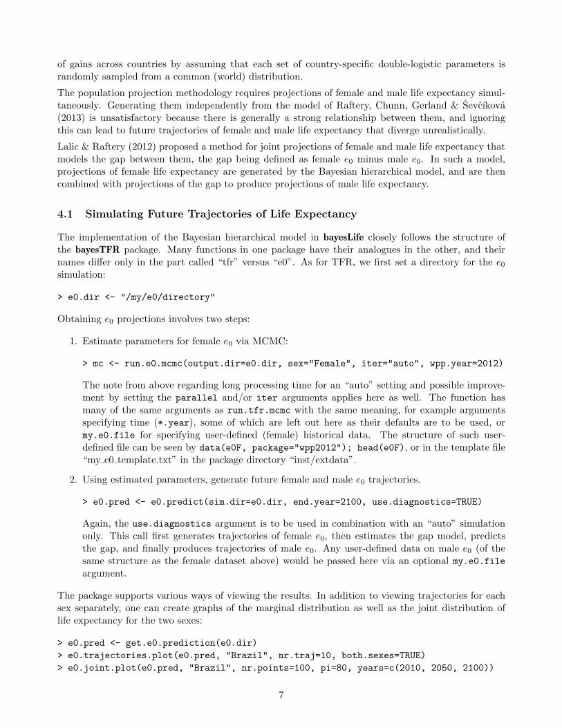
The package supports various ways of viewing the results. In addition to viewing trajectories for eachsex separately, one can create graphs of the marginal distribution as well as the joint distribution oflife expectancy for the two sexes:

> e0.pred <- get.e0.prediction(e0.dir)

> e0.trajectories.plot(e0.pred, "Brazil", nr.traj=10, both.sexes=TRUE)

> e0.joint.plot(e0.pred, "Brazil", nr.points=100, pi=80, years=c(2010, 2050, 2100))

7

●

●

●

●

●

●

●

●

●

●

●●

1950 2000 2050 2100

5060

7080

9010

0Brazil

Year

Life

exp

ecta

ncy

at b

irth

●

●

●

●

●

●●

●

●

●

●

●

●

●

female median80% PI femaleobserved female e0male median80% PI maleobserved male e0

60 70 80 90 100 110 120

6070

8090

100

110

120

Brazil

Female life expectancy

Mal

e lif

e ex

pect

ancy

2005−20102045−20502095−2100

Figure 4: Future e0 marginal trajectories (left) and joint female-male distribution for three differenttime points (right) with 80% probability interval for Brazil.

The results are shown in Figure 4. Other functions for exploring results are available in bayesLife, suchas creating maps, or generating plots for all countries at once.

5 Population Projection

5.1 Producing Future Population Trajectories

As mentioned in Section 2, probabilistic population projections implemented in bayesPop incorporatetwo probabilistic components, namely TFR and sex-specific e0. For each country, the prediction func-tion applies the cohort component method to each trajectory, keeping the remaining input componentsconstant.

Thus in standard cases, to generate future population trajectories, all one needs to do is to point thecode to the place on disk where TFR and e0 are stored, in our case the tfr.dir and e0.dir directories.The results are stored in a separate directory:

> pop.dir <- "/my/pop/directory"

> pop.pred <- pop.predict(end.year=2100, start.year=1950, present.year=2010,

wpp.year=2012, output.dir=pop.dir, nr.traj=1000,

inputs=list(tfr.sim.dir=tfr.dir,

e0F.sim.dir=e0.dir, e0M.sim.dir="joint_"))

The keyword “joint ” directs the function to extract the male e0 projections from the female simulationdirectory, i.e. it indicates that e0 was simulated jointly for female and male. The start.year determinesthe first time period for observed death rates to be used in the Lee-Carter method, and present.year

is the time period of the initial population data. Obviously, end.year cannot go beyond the end yearused in TFR and e0 projections, nor beyond the end year of other projection inputs, such as migration.If the number of trajectories to be produced (nr.traj) is smaller than the number of available TFR and

8

●

●

●

●

●

●

●

●

●

●

●

●

●

1950 2000 2050 2100

4000

0060

0000

8000

0010

0000

014

0000

0

ChinaP

opul

atio

n pr

ojec

tion

median80% PI95% PIobserved

020

000

4000

060

000

8000

010

0000

1200

00

China 2095−2100

Pop

ulat

ion

proj

ectio

n

0−4

5−9

10−

1415

−19

20−

2425

−29

30−

3435

−39

40−

4445

−49

50−

5455

−59

60−

6465

−69

70−

7475

−79

80−

8485

−89

90−

9495

−99

100−

104

105−

109

110−

114

115−

119

120−

124

125−

129

130+

median80% PI

2010

Figure 5: Projected trajectories for China. Left panel shows the population projection by time; theright panel shows the population projection by age for 2100 (red lines) and for the present year, 2010,(blue line).

e0 trajectories, these are equidistantly thinned. The deterministic input components are taken fromthe given wpp package, here wpp2012. However, the inputs argument allows one to overwrite each ofthem using tab-delimited text files. Instead of one’s own projection of TFR and e0, it is possible to usethe UN-predicted quantiles (included in the wpp2012 package) by leaving all the *.sim.dir elementsequal to NULL (the default). An optional logical argument keep.vital.events can be used for storingadditional data generated during projection, such as births and deaths. By default these are not kept,as it more than doubles the amount of data stored.

To access such population prediction objects in a later session one can use:

> pop.pred <- get.pop.prediction(pop.dir)

5.2 Viewing Population Trajectories

Population trajectories can be viewed on a country-specific basis. A simple summary function gives aquick look at various quantiles of the country’s projections, e.g.:

> summary(pop.pred, country="Italy")

The following code shows how to create plots of trajectories by time as well as by age, including addingcurves to existing plots. Results are shown in Figure 5.

> country <- "China"

> pop.trajectories.plot(pop.pred, country=country, sum.over.ages=TRUE, nr.traj=50)

> pop.byage.plot(pop.pred, country=country, year=2100, nr.traj=50, pi=80, ylim=c(0,130000))

> pop.byage.plot(pop.pred, country=country, year=2010, add=TRUE, show.legend=FALSE, col="blue")

> legend("topright", legend=2010, col="blue", lty=1, bty="n")

If sum.over.ages in pop.trajectories.plot is FALSE, separate plots for each age group are generated.The function also accepts arguments for specifying sex and age where age is defined as an index to

9

Male Female

6300 4400 2500 630 630 1900 3200 5100

0−45−9

10−1415−1920−2425−2930−3435−3940−4445−4950−5455−5960−6465−6970−7475−7980−8485−8990−9495−99

100−104

0−45−910−1415−1920−2425−2930−3435−3940−4445−4950−5455−5960−6465−6970−7475−7980−8485−8990−9495−99100−104median

95% PI80% PI2005−2010

Population in Russian Federation: 2075−2080Male Female

0.06 0.04 0.02 0 0.01 0.03 0.05

0−45−9

10−1415−1920−2425−2930−3435−3940−4445−4950−5455−5960−6465−6970−7475−7980−8485−8990−9495−99

100−104105−109110−114

0−45−910−1415−1920−2425−2930−3435−3940−4445−4950−5455−5960−6465−6970−7475−7980−8485−8990−9495−99100−104105−109110−114

Population in Russian Federation: 2095−2100

median80% PI2010−201580% PI1945−1950

Figure 6: Probabilistic population pyramid for Russia: a classic type comparing two time periods onthe left, and trajectory type comparing three time periods on a proportion scale on the right.

the vector (0-4, 5-9, 10-14, . . ., 125-129, 130+), thus of length 27. A graph for male population aged0-14 would have arguments sex="male", age=1:3, or women in child bearing age would be defined assex="female", age=4:10.

Numerical analogous to the trajectory plots is implemented in the functions pop.trajectories.tableand pop.byage.table, respectively. Trajectory plots can be created for all countries at once usingpop.trajectories.plotAll and pop.byage.plotAll.

5.3 Probabilistic Population Pyramids

The package supports plotting probabilistic population pyramids for given country and one or moregiven years. There are two different kinds of pyramids – a classic pyramid consisting of boxes, anda so called trajectory pyramid which is created using age trajectories such as the ones on the right inFigure 5. The classic pyramid can display projections for up to two years in one pyramid with one setof probability intervals; the trajectory pyramid can include any number of years and any number ofprobability intervals. Here is an example of generating the two pyramid types, see Figure 6:

> country <- "Russian Federation"

> pop.pyramid(pop.pred, country, year=c(2080, 2010))

> pop.trajectories.pyramid(pop.pred, country, year=c(2100, 2015, 1950),

nr.traj=0, proportion=TRUE, age=1:23, pi=80)

Here the trajectory pyramid uses the argument proportion to switch the x-axis to a proportionalscale, which is useful when comparing pyramids from different time periods. Both functions also acceptvarious arguments for changing the appearance of the pyramids, such as colors, height and thicknessof boxes etc.

In addition to creating pyramids for the results of the pop.predict function, both pyramid functionscan also be applied to any user-defined data that can be fitted into a pyramid data structure. See thepackage documentation for more detail.

10

5.4 bayesPop Expressions

So far we have explored data resulting directly from the pop.predict function, which provides infor-mation about sex- and age-specific population projections. It is often of interest, however, to analysevarious derivations and transformations of these quantities, such as potential support ratio, mean age ofchild bearing, median age etc. For this purpose, the package implements a simple expression languagethat allows one to compute such quantities on the fly.

A bayesPop expression is a collection of basic components connected via usual arithmetic operators andcombined using parentheses. Standard R functions and pre-defined functions can be also used withinexpressions.

A basic component of an expression is a character string consisting of four sub-strings, the first two ofwhich are mandatory. They must be in the following order:

1. Measure identification. The following upper-case characters are currently allowed: P for Popula-tion, D for Deaths, B for Births, S for Survival ratio, F for Fertility rate, M for Mortality rate,Q for probability of dying, and G for net miGration. All but the P and G indicators can be usedonly if keep.vital.events was set to TRUE when generating predictions. P and G are alwaysavailable.

2. Country part which can be either a numerical country code or two- or three-character ISO 3166code, or characters “XXX” which serves as a wildcard for a country code. For example, “P528”,“PNL”, and “PNLD” are all expressions for the total population of the Netherlands.

3. Sex sub-string (optional) which is either “ F” or “ M”, specifying female or male indicator, re-spectively. An expression consisting of two basic components “P528 F / P528” gives the ratio ofthe female population to the total population in the Netherlands.

4. Age sub-string (optional). If used, the basic component is concluded by an array of age indices.Such an array is enclosed by either brackets (“[ ]”) or curly braces (“{ }”). The former invokes asummation of counts over given ages, and the latter is used when no summation is desired. If theage sub-string is missing, counts are automatically summed over all ages. To use all ages withoutsumming, empty curly braces can be used. For example, the female population of India of childbearing age can be expressed as “PIND F[4:10]”. Indicators S, M and Q allow an index −1 whichcorresponds to the age group 0–1, and an index 0 which corresponds to the age group 1–4.

Not all combinations of the four parts above make sense. For example, fertility rate can be combinedonly with female sex and a subset of the age groups, namely child bearing ages (indices 4 to 10). Birthsare also restricted to those age groups. As another example, all the rate-like indicators (S, F, M, Q)should include all four components, as summing over sexes or age groups is meaningless for this typeof measure.

Basic components can be combined using arithmetic operations, R functions, or pre-defined functionsin the package. Among the most useful pre-defined functions are gmedian, gmean for group median andgroup mean, respectively, and pop.apply for applying a function along the age axis of the data. Hereare a few examples of bayesPop expressions and their use in the package functions (please refer to thehelp page ?pop.expressions for more details):

Summarising by time: These country-specific expressions can be used in pop.trajectories.plot

and pop.trajectories.table.

• Median age of France:“pop.apply(PFR{}, gmedian, cats=seq(0, by=5, length=28))”

11

Potential support ratio in 2045−2050

1.28 1.93 2.18 2.48 2.82 3.41 4.25 5.95 8.12 9.57 15.1

Figure 7: World map of the median projection of potential support ratio in 2045-2050.

• Average age of women in the USA in child bearing age:“pop.apply(PUSA F{4:10}, gmean, cats=seq(15, by=5, length=8))”

• Ratio of German to French total population: “PDE / PFR”

• Potential support ratio of India: “PIND[5:13] / PIND[14:27]”

Summarising by age: Country-specific expressions that can be used in pop.byage.plot andpop.byage.table in which time must be given.

• Log of male mortality rate for Spain: “log(MES M{})”• Migration per capita in the Netherlands: “GNL{} / PNL{}”• Number of births by mother’s age per woman of the same age in Hungary:

“BHU{} / PHU F{4:10}”

All countries: The character string “XXX” can be used in functions for plotting maps, such aspop.map and pop.map.gvis, or a function write.pop.projection.summary for exporting pro-jection results into an ASCII file. These expressions should be constructed the same way asthe “by time” expressions above, but the country code should be replaced by “XXX”, e.g. thefollowing code generates the map in Figure 7 for potential support ratio:

> pop.map(pop.pred, expression = "PXXX[5:13] / PXXX[14:27]", year=2050,

main="Potential support ratio in 2045-2050", numCats=20)

The same applies when using expressions in pop.trajectories.plotAll. Function pop.byage.plotAll

accepts expressions containing “XXX” constructed as expressions “by age” above.

12

● ● ● ● ● ● ● ● ● ● ● ●●

1950 2000 2050 21000e+

002e

+06

4e+

066e

+06

AFRICA

Pop

ulat

ion

proj

ectio

n

median80% PI95% PIobserved

●

●

●

●

●

●

●

●

●● ●

●●

1950 2000 2050 21005500

0065

0000

7500

00 EUROPE

Pop

ulat

ion

proj

ectio

n

median80% PI95% PIobserved

●●

●●

●●

●●

●●

●●

●

1950 2000 2050 2100

2e+

053e

+05

4e+

055e

+05

6e+

05

NORTHERN AMERICA

Pop

ulat

ion

proj

ectio

n

median80% PI95% PIobserved

●●

●●

●

●

●

●

●

●

●●

●

1950 2000 2050 21002e

+06

4e+

066e

+06

ASIA

Pop

ulat

ion

proj

ectio

n

median80% PI95% PIobserved

Figure 8: Population trajectories for aggregated regions.

5.5 Aggregations

In addition to producing population estimates and projections at the country level, the UN also pro-vides projections for numerous country aggregates of interest, such as geographic regions and tradingblocs. bayesPop offers two methods for producing aggregations, namely an Independence method anda Regional method. The Independence method treats population trajectories as independent betweencountries, and thus, the aggregation is accomplished by simply summing population counts on eachtrajectory across countries of the regions in question. In the Regional method, aggregations are gener-ated using the cohort component method as described in Section 2 using aggregated input components.Here is an example of aggregating over continents and over the whole world:

> pop.aggr <- pop.aggregate(pop.pred, method="independence",

# World, Africa, Europe, Northern America, Asia, Latin Am.

regions=c(900, 903, 908, 905, 935, 904), verbose=TRUE)

The region codes must correspond to the column “area code” of the UNlocations dataset in thewpp2012 package. Alternatively, user-defined aggregations are also supported, see ?pop.aggregate

for more information.

Results of the aggregation are stored in the same directory as pop.pred and can be retrieved in latersessions by

> get.pop.aggregation(pop.dir)

Both functions above accept an argument name. Thus, one can label an aggregation and keep multipleaggregation objects in the same directory.

The stored data have the same structure as the non-aggregated prediction object. Thus, any of the sum-marising and plotting function described in the previous sections can be used, including in combination

13

Male Female

0.048 0.038 0.029 0.019 0.01 0 0.01 0.019 0.029 0.038 0.048

0−4

5−9

10−14

15−19

20−24

25−29

30−34

35−39

40−44

45−49

50−54

55−59

60−64

65−69

70−74

75−79

80−84

85−89

90−94

95−99

100−104

0−4

5−9

10−14

15−19

20−24

25−29

30−34

35−39

40−44

45−49

50−54

55−59

60−64

65−69

70−74

75−79

80−84

85−89

90−94

95−99

100−104median95% PI80% PI2005−2010

Population in WORLD: 2095−2100

0.0

0.2

0.4

0.6

African population to world population 2095−2100

0−4

5−9

10−

1415

−19

20−

2425

−29

30−

3435

−39

40−

4445

−49

50−

5455

−59

60−

6465

−69

70−

7475

−79

80−

8485

−89

90−

9495

−99

100−

104

105−

109

110−

114

115−

119

120−

124

125−

129

130+

median80% PI

2010

Figure 9: Left panel: Population pyramid for the world in 2010 and 2100. Right panel: Proportion ofAfricans to the world population by age in 2100 and the same indicator in 2010 (blue line).

with expressions:

> par(mfrow=c(2,2))

> for (region in c(903, 908, 905, 935))

pop.trajectories.plot(pop.aggr, region, sum.over.ages=TRUE, nr.traj=50)

> pop.pyramid(pop.aggr, 900, year=c(2100, 2010), proportion=TRUE)

> pop.byage.plot(pop.aggr, expression="P903{} / P900{}", year=2100, pi=80,

main = "African population to world population 2095-2100",

nr.traj=50)

> pop.byage.plot(pop.aggr, expression="P903{} / P900{}", year=2010,

nr.traj=0, add=TRUE, show.legend=FALSE, col="blue")

> legend("topright", legend=2010, col="blue", lty=1, bty="n")

Resulting graphs are shown in Figures 8–9. Note that several of the countries in Africa are experiencinggeneralised HIV/AIDS epidemics, and for these countries the projected life expectancies in WPP 2012were generated by bayesLife using different settings than used for other countries. The results shownhere are based on the life expectancies published in WPP 2012.

6 Graphical User Interface

6.1 bayesDem: Bayesian Demographer

A graphical user interface for bayesTFR, bayesLife, and bayesPop is implemented in the R packagebayesDem (Bayesian Demographer). One can generate probabilistic projections of TFR, life expectancy,and combine those results into probabilistic population projections from a single interface. In addition,it offers functionality for exploring results, such as trajectories, maps, population pyramids and others.

14

Bayesian Demographer can be loaded into and started from the R interface by

> library(bayesDem)

> bayesDem.go()

Figure 10: Bayesian Demographer: Graphical user interface for bayesTFR, bayesLife, and bayesPop.

which opens the main window of the GUI (see Figure 10). There are three upper level tabs each ofwhich corresponds to one of the underlying packages. Each package operates on its own directory whichare entered in the “Simulation directory” field on the top of the GUI. The “Info” button beside it givesinformation about estimation and projection objects already stored in the given directory.

Each main tab is organised into sub-tabs, each of which corresponds to a function (or group of relatedfunctions) of the corresponding package. They are ordered from left to right in the same way an analystwould progress on his/her road to population projection along the blue arrows in Figure 1.

In the bottom right corner there is usually a button that invokes the actual function after collectingits arguments from the workspace. A button “Generate Script” shows how the function is invoked.

15

The user can use this functionality to copy and paste function calls into a batch file which can be thenprocessed outside of the GUI. This is especially useful and recommended for time-consuming processes,such as MCMC runs or generating predictions. In order to help users with the meaning of the variousinputs, there is a “Help” button in the bottom left corner which shows help pages for the underlying Rfunction(s).

All functions described in this paper and many more can be accessed through the GUI.

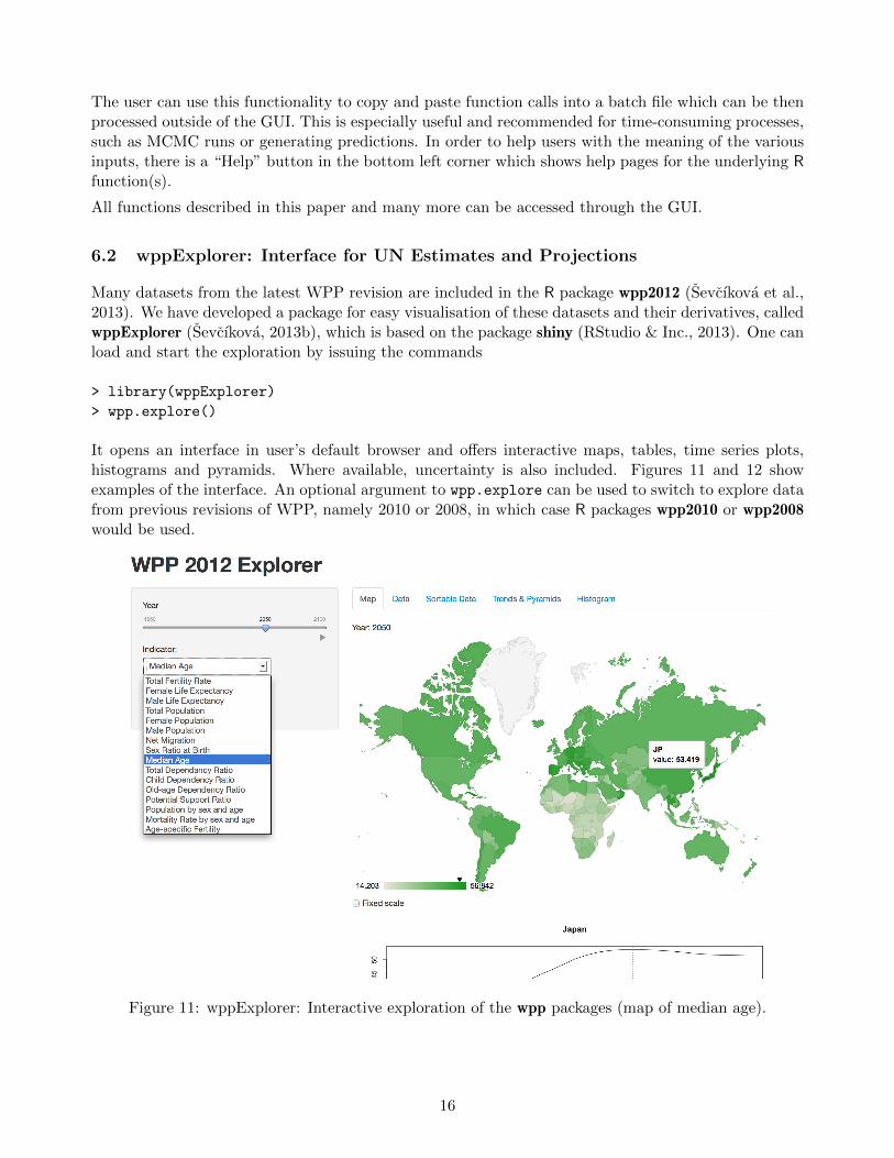
6.2 wppExplorer: Interface for UN Estimates and Projections

Many datasets from the latest WPP revision are included in the R package wpp2012 (Sevcıkova et al.,2013). We have developed a package for easy visualisation of these datasets and their derivatives, calledwppExplorer (Sevcıkova, 2013b), which is based on the package shiny (RStudio & Inc., 2013). One canload and start the exploration by issuing the commands

> library(wppExplorer)

> wpp.explore()

It opens an interface in user’s default browser and offers interactive maps, tables, time series plots,histograms and pyramids. Where available, uncertainty is also included. Figures 11 and 12 showexamples of the interface. An optional argument to wpp.explore can be used to switch to explore datafrom previous revisions of WPP, namely 2010 or 2008, in which case R packages wpp2010 or wpp2008would be used.

Figure 11: wppExplorer: Interactive exploration of the wpp packages (map of median age).

16

Figure 12: wppExplorer: Interactive exploration of the wpp packages (Population pyramid of Chinaand India).

7 Discussion

We have shown the basic functionality of our demographic packages, namely bayesTFR, bayesLife,bayesPop, bayesDem, and wppExplorer. They can be used to reproduce some of the UN WPP 2012demographic projections and visualize results. The packages offer additional features not mentionedin this paper, such as special handling of small areas, imputing missing values, analysing MCMCs,exporting projections, etc. We refer the reader to the corresponding package documentation for moredetails.

In the World Population Prospects, the UN currently publishes estimates back to 1950, and populationprojections are based on them. However, data are available for some countries long before 1950, insome cases back to 1750, and these can be taken into account in the projections if desired. We haveshown how to do this.

As currently implemented, our software and methods for TFR and life expectancy are for nationalprojections, with country as the unit of analysis. However, the same conceptual approach could beused to produce subnational projections for administrative subregions (states, provinces, counties, etc.)of a country. One way of doing this would be to specify a three-level hierarchical model for the world,with world, country and subregion as the levels. A more approximate but easier approach would be touse the current software in the following way. Recast the “world” as the country, and the “countries” asthe subregions. Then use the posterior distribution of the world parameters from the full (world-wide)run to inform the prior parameters used in the country-specific run. Precisely how to do this wouldrequire some further specification and care.

Acknowledgements: This work was supported by the Eunice Kennedy Shriver National Instituteof Child Health and Human Development under grants R01 HD054511 and R01 HD070936. Raftery’sresearch was also supported by Science Foundation Ireland E.T.S. Walton visitor award 11/W.1/I2079.

17

Disclaimer: The views and opinions expressed in this paper are those of the authors and do notnecessarily represent those of the United Nations. The contents has not been formally edited andcleared by the United Nations. The designations employed in this paper do not imply the expression ofany opinion whatsoever on the part of the Secretariat of the United Nations concerning the legal statusof any country, territory or area or of its authorities, or concerning the delimitation of its frontiers orboundaries.

References

Alkema, L., Raftery, A. E., Gerland, P., Clark, S. J., Pelletier, F., Buettner, T., & Heilig, G. K. (2011).Probabilistic projections of the total fertility rate for all countries. Demography, 48, 815–839.

Ihaka, R. & Gentleman, R. (1996). R: A language for data analysis and graphics. Journal of Compu-tational and Graphical Statistics, 5, 299–314.

Lalic, N. & Raftery, A. E. (2012). Joint probabilistic projection of female and male life expectancy.Presented at the annual meeting of Population Association of America. http://paa2012.princeton.edu/abstracts/120140.

Lee, R. D. & Carter, L. (1992). Modeling and forecasting the time series of US mortality. Journal ofthe American Statistical Association, 87, 659–671.

Lee, R. D. & Tuljapurkar, S. (1994). Stochastic population forecasts for the United States: Beyondhigh, medium, and low. Journal of the American Statistical Association, 89, 1175–1189.

National Research Council (2000). Beyond Six Billion: Forecasting the World’s Population. Washing-ton, D.C.: National Academy Press.

Raftery, A. E., Alkema, L., & Gerland, P. (2013). Bayesian population projections for the UnitedNations. Statistical Science, in press.

Raftery, A. E., Chunn, J. L., Gerland, P., & Sevcıkova, H. (2013). Bayesian probabilistic projectionsof life expectancy for all countries. Demography, 50, 777–801.

Raftery, A. E., Li, N., Sevcıkova, H., Gerland, P., & Heilig, G. K. (2012). Bayesian probabilisticpopulation projections for all countries. Proceedings of the National Academy of Sciences, 109,13915–13921.

RStudio & Inc. (2013). shiny: Web Application Framework for R. R package version 0.7.0.

United Nations (1956). Manual III: Methods for population projections by sex and age. New York, NY:Dept. of Economic and Social Affairs, Population Division. Vol. 25 - Population Studies.

United Nations (1989). The United Nations Population Projection Computer Program : A User’sManual. New York, NY: Dept. of Economic and Social Affairs, Population Division.

United Nations (2013). World Population Prospects: The 2012 Revision. New York, NY: UnitedNations.

Sevcıkova, H. (2013a). bayesDem: Graphical User Interface for bayesTFR, bayesLife and bayesPop. Rpackage version 2.3-2.

Sevcıkova, H. (2013b). wppExplorer: Explorer of World Population Prospects. R package version 1.0-3.

18

Sevcıkova, H., Alkema, L., & Raftery, A. E. (2011). bayesTFR: An R package for probabilistic projec-tions of the total fertility rate. Journal of Statistical Software, 43, 1–29.

Sevcıkova, H., Gerland, P., Andreev, K., Li, N., Gu, D., & Spoorenberg, T. (2013). wpp2012: WorldPopulation Prospects 2012. R package version 2.0-0.

Sevcıkova, H. & Raftery, A. (2013a). bayesPop: Probabilistic Population Projection. R package version4.1-1.

Sevcıkova, H. & Raftery, A. E. (2013b). bayesLife: Bayesian Projection of Life Expectancy. R packageversion 2.0-1. Original WinBugs code written by Jennifer Chunn.

Whelpton, P. K. (1928). Population of the United States, 1925–1975. American Journal of Sociology,31, 253–270.

Whelpton, P. K. (1936). An empirical method for calculating future population. Journal of the Amer-ican Statistical Association, 31, 457–473.

19