bayesian probabilistic approach for predicting...

Bayesian Probabilistic Approach for Predicting BackboneStructures in Terms of Protein BlocksA. G. de Brevern,1* C. Etchebest,1,2 and S. Hazout1

1Equipe de Bioinformatique Genomique et Moleculaire, INSERM U436, Universite Paris 7, Paris, France2Laboratoire de Biochimie Theorique, UPR 9080 CNRS, Institut de Biologie Physico-Chimique, Paris, France

ABSTRACT By using an unsupervised clusteranalyzer, we have identified a local structural alpha-bet composed of 16 folding patterns of five consecu-tive Ca (“protein blocks”). The dependence thatexists between successive blocks is explicitly takeninto account. A Bayesian approach based on therelation protein block-amino acid propensity is usedfor prediction and leads to a success rate close to35%. Sharing sequence windows associated withcertain blocks into “sequence families” improvesthe prediction accuracy by 6%. This prediction accu-racy exceeds 75% when keeping the first four pre-dicted protein blocks at each site of the protein. Inaddition, two different strategies are proposed: thefirst one defines the number of protein blocks ineach site needed for respecting a user-fixed predic-tion accuracy, and alternatively, the second onedefines the different protein sites to be predictedwith a user-fixed number of blocks and a chosenaccuracy. This last strategy applied to the ubiquitinconjugating enzyme (a/b protein) shows that 91% ofthe sites may be predicted with a prediction accu-racy larger than 77% considering only three blocksper site. The prediction strategies proposed im-prove our knowledge about sequence-structure de-pendence and should be very useful in ab initioprotein modelling. Proteins 2000;41:271–287.© 2000 Wiley-Liss, Inc.

Key words: protein backbone structure; unsuper-vised classifier; structure-sequence rela-tionships; structure prediction; proteinblock; Bayesian approach; predictionstrategies

INTRODUCTION

The protein sequence contains the whole information ofthe protein three-dimensional (3D) structure. Proteinscannot fold into unlimited number of structural motifs.1,2

Yet our lack of understanding of the physicochemical andkinetic factors involved in folding prevent us from advanc-ing from knowledge of the primary sequence to reliablepredictions of the biologically active 3D structure. The firstlevel of the protein structure is the secondary structurecharacterized in terms of a-helix, b-strand, and unrepeti-tive coil. A thousand different prediction algorithms havebeen developed, e.g., statistical methods like the pioneerGOR3,4 or neural networks like the well-known PHD5 and

the more recent work of Chandonia and Karplus.6,7 Theaccuracy of these works were strongly increased with theaddition of the multiple sequences alignment in the neuralnetworks,8 probabilistic approach,9 or computational infor-mative encoding.10 The increase in the entries in thebiologic databases may permit an increase in the predic-tion rate.11

Concerning the 3D structure, the ab initio proteinfolding algorithms, using only energetic or physicochemi-cal parameters, were limited to small proteins.12–14 Numer-ous studies describe the ab initio modeling of a 3Dstructure from the sole knowledge of its primary structure.However, due to actual weakness of the prediction rate,this determination is still an open field.

The results obtained in the recent CASP III meeting arethe best witnesses of such tentative findings.15 The compat-ibility of the sequence versus known structures is analternative approach to find the best approximation of theprotein fold.16,17 Most of the methods for finding thefolding state of a protein are mainly based on the use of the3D structure of homologous proteins combined with simpli-fied spatial restraints, statistical analysis, and physico-chemical constraints.18,19

Recently, the use of fragment library20 more detailedthan three-states and based on the most frequent localstructural motifs (in terms of polypeptide backbone) en-countered in the ensemble of 3D structure protein data-base had led to improved results21,22 within a knowledge-based ab initio method.23

Clearly, the main difficulty to overcome resides alongthe pathway going from the secondary structure predictionto the tertiary structure prediction. In this spirit, the studyof the local conformations of proteins had a long historyprincipally based on the study of the classic repetitivestructures. We can notice interesting works such as thosebased on the geometric and sequential characterization ofa-helices24 or discrimination between the different types ofb-turns.25 Most algorithms that described global conforma-tions of the proteins used this simple structural alpha-bet.26–28 Recently, with the constant augmentation of theProtein Data Bank, automatic researches designed to

*Correspondence to: Alexander de Brevern, Equipe de Bioinforma-tique Genomique et Moleculaire, INSERM U436, Universite Paris 7,case 7113, 2, place Jussieu, 75251 Paris cedex 05, France. E-mail:[email protected]

Received 6 January 2000; Accepted 12 June 2000

PROTEINS: Structure, Function, and Genetics 41:271–287 (2000)

© 2000 WILEY-LISS, INC.

determine families of specific coils have been carriedout.29–31

Among the different works concerning the definition of astructural alphabet (the consensus structural patternswill be labelled protein blocks, or PBs), two main types oflibraries of PBs can be distinguished: those composed of ahigh number (around 100) of protein blocks for describingprotein structures or those characterized by a limitednumber of fold prototypes (4 to 13).

In the first type, the use of small blocks (fragments of sixamino acids) for rebuilding a protein structure had begunwith the work of Unger et al.32 using the RMSD (root meansquare deviation) as criterion. The authors have identifiedabout 100 building blocks that could replace about 76% ofall hexamers with an error of less than 1 Å. Schuchhardt etal.33 similarly obtained a library of 100 structural motifsby an unsupervised learning algorithm from the series ofdihedral angles. These libraries are adequate for approxi-mating a 3D protein structure; however, they are noteasily usable for prediction.

In the second type of approaches, Rooman et al. definerecurrent folding motifs by a clustering algorithm usingthe RMSD on distances between selected backbone at-oms.34 They described 16 motifs (embedded by groups of 4)of different lengths (from 4 to 7 residues). This smallalphabet is directly related to the four classes of secondarystructure (a-helix, b-strand, turn, and coil) and permitsdistinction between b-bulges and b-strands. Fetrow et al.developed an autoassociative artificial neural network(autoANN) to define six clusters corresponding to supersec-ondary structures encompassing the classic secondarystructures.35

Bystroff and Baker have generated a high number ofsimilar short folds of different lengths and then groupedthem into 13 clusters for a prediction approach.20 A recentapproach performed by Camproux et al.36 takes account ofthe succession of the folds in the training by HiddenMarkov Model (HMM)37 and has allowed the definition ofa library of 12 blocks of 4 Ca. This approach, as expected,allows the assessing of the transition frequencies betweenthe blocks.

In this study, the aims consist (1) in building a set ofstructural blocks able to approximate at best the differentstructural patterns observed along the protein backbones,and (2) in predicting the local 3D structure of the backbonein terms of PBs from the knowledge of the sequence.Identification of the different structural blocks is per-formed by an unsupervised cluster analyzer, taking intoaccount the sequential dependence of the blocks; this pointis also considered in HMM.37

After this phase of training performed on a givennonredundant protein database, we can tackle the prob-lem of the prediction of these structural blocks from theknowledge of the protein sequence. From a given library ofPBs, amino acid preferences for different positions alongthe fragment can be extracted for each fold pattern. So, byusing Bayes theorem, these probabilities may be furtherused to predict the structural motifs able to be adopted bya given protein chain. The Bayesian probabilistic approach

is largely applied in this type of study, for instancepredicting solvent accessibility,38 secondary structure,9 orcharacterization of biologic pathways from sequences tofunctions.39

In this study, we have worked in different aspects toimprove the PB prediction: 1 Protein Block—n Sequences:Associating one protein block with one class of sequences isa restrictive point of view. A same fold pattern (or PB) maybe associated with different types of sequences, So, wehave built a procedure for splitting the set of sequences (or“windows”) encompassing a given PB into a fixed numberof subsets showing (called “sequence families”) at bestdifferent amino acid distributions in each window site. 1Sequence—n Protein Blocks: It is the inverse concept.Similar sequences are not always associated with the samefold,40 but with different “possible” folds. So, we can devisea “fuzzy model” in which we have a certain probability forfinding the true PB (this one that approximates at best thelocal structure of the backbone) among the proposed PBs.Concerning the existence of this “fuzzy model,” we ought tocheck that the true PB is present among the solutions ofthe r first ranks (i.e., having the best prediction scores)provided by the Bayesian approach.

We will show the interest of an entropy-based index todiscriminate different zones of the protein with highprobabilities of prediction. With the scoring schema andthe index control, two main directions have been explored.The first one, called “global strategy,” consists of locallydetermining the optimal number of protein blocks to beselected after fixing the prediction rate for the wholeprotein sites. So, the number of selected solutions perposition may be variable. In contrast, the second direction,called “local strategy,” scans the protein sequence with afixed number of solutions (i.e., a constant number ofprotein blocks per position) and determines the regionsable to be predicted with this given number and with afixed prediction accuracy. In this way, the prediction onlyconcerns these protein regions. Consequently, two predic-tion strategies are available; they both provide informa-tion complementary and enough for a former use in abinitio modeling.

MATERIALS AND METHODSProtein Database

A total of 342 proteins are selected in a database ofnonhomologous protein structures (less than 25% of se-quence similarity).41,42 For each protein, we have storedthe series of dihedral angles and the primary sequences.Each protein backbone is transformed into a signal corre-sponding to the series of the dihedral angles (fi, ci). So, thedatabase is composed of 342 signals. For the analysis, theproteins are splitting up in fragments of five consecutiveresidues to define the protein blocks. We have divided theset of proteins into two subsets, one of 228 proteins usedfor the training stage (i.e., the step allowing the definitionof the protein blocks and the relationships between theprotein blocks and the amino acid composition), the otherone of 114 proteins for the stage of prediction accuracyassessing.

272 A. G. DE BREVERN ET AL.

The proteins are classified according to the nomencla-ture using the criteria of Michie and co-workers,27 whichallows division of the protein set into four classes all a, allb, a/b, and unclassified. The secondary structures aredefined by a consensus assignment based on three algo-rithms.43

Coding of Five-Residue Chains

A conventional approach for describing the backbone ofa protein consists in converting the peptide coordinatesinto a series of backbone dihedral angles f, c, and v. In thestudy, we will neglect the variation of the v angle whosevalues vary around 0 degrees or 180 degrees.44 We havelimited the analysis to fragments of five residue lengthbecause it is sufficient to describe more than an short helixa (four residues24) and a minimal b structure (threeresidues43). A set of five consecutive peptides is an accept-able structural pattern to compute locations of hydrogenbonds between them. The link between the two successivecarbons (Can, Can11) located at the nth and (n 1 1)thpositions in the protein sequence is defined by the dihedralangles cn of Can and fn11 of Can11. A series of M peptidesis defined by a signal of 2(M 2 1) values. So a fragment offive residues (M 5 5) centered at the alpha-carbon Can isdisplayed by a vector of eight dihedral angles: V(cn22,fn21, cn21, fn, cn, fn11, cn11, fn12) associated with theconsecutive carbons Can22, Can21, Can, Can11, Can12,respectively.33 The fragments used are overlapped. Hence,a protein of length L is described by L 2 4 fragments. Thisleads to a database of 86,628 dihedral vectors correspond-ing to the 342 protein signals.

Training by an Unsupervised Cluster Analyzer

The goal is to define a structural alphabet for coding thelocal 3D structure of protein backbones. This alphabet iscomposed of “proteins blocks” (PBs), which representaverage patterns of the backbone fragments extractedfrom the database. Each one is defined by a vector of2(M 2 1) values of dihedral angles like the fragments ofthe database.

Principle of the unsupervised cluster analyzer

The method uses the principle of the self-organizedlearning of the Kohonen network (or self-organized maps,often noted SOM45,46), i.e., by reading a certain number oftimes (called “cycles”), the totality of the vector database todefine the “weights” of the neurons. In the terminology ofthe SOMs, the neurons and the weights correspond to aclass of objects (in our study, protein blocks) and theassociated information (herein, the average dihedral vec-tors), respectively. We have defined two steps in thetraining procedure. The first one consists of learning theprotein blocks, by only considering the local protein struc-ture (i.e., series of five carbons a), and the second one, byintroducing constraints on the transitions between theprotein blocks to favor a Markovian process of order 1, asthe Hidden Markov Models (HMM37) to use the naturalsequence of the protein structure. Our approach does notset any hypothesis of a priori distributions of the data(herein, the dihedral vectors).

Dissimilarity measure

The choice of the measure of dissimilarity between theM-residues fragments is essential for defining PBs strictlydifferent in the training phase. In our study, the vectorassociated with a fragment (called “dihedral vectors”) is aseries of dihedral angles. So the chosen dissimilaritymeasure between two vectors V1 and V2 of dihedral anglesis defined as the Euclidean distance among the M 2 1links, the RMSDA (root mean square deviations on angu-lar values33):

RMSDA~V1, V2!

5Î O

i51

i5M21

@ci~V1! 2 ci~V2!#2 1 @fi11~V1! 2 fi11~V2!#

2

2~M 2 1!

where {fi(V1), ci11(V1)}(resp. fi(V2), ci11(V2)) denotes theseries of the (2M 2 1) dihedral angles for V1 (resp. V2).The angle differences are computed modulo 360 degrees.So in the training, this distance is used for assessing thedissimilarity of any fragment of the database with thedifferent PBs.

Description of the training approach

Each protein block PBk considered as a neuron isinitially defined by a vector W(k) of eight dihedral angles (kdenoting a given PB), either defined by a series of fourdihedral angle pairs drawn in a Ramachandran diagramor randomly drawn in the database of vectors. Initially thenumber B of PBs is arbitrarily fixed. We assume that, atthe beginning of the training, no transitions exist betweenthese structural blocks.

a: First training. In the first step of the trainingdescribed in Figure 1, we consecutively read the dihedralvectors from a signal (representing a given protein). Forevery dihedral vector V(m), m denotes the mth vector inthe signal. The sequence of the dihedral vectors observedalong the proteins is kept. We search for, among the Bpossible PBs, this one, PBk, whose vector W(k) is theclosest one according to the dissimilarity measure previ-ously defined (minimal RMSDA). Then the vector W(k) ofthis closest PB is changed into:

W~k! 1 ~V~m! 2 W~k!! z n~c!

where n(c) is a coefficient (initially taken low, n0 5 0.02)decreasing during the training. n(c) is a function of cdenoting the number of vectors read during the training:

n~c! 5 n0/~1 1 t z c!

where t is arbitrarily fixed to 1/N (i.e., the number ofdihedral vectors, here N 5 56,442) so that n(c) is reducedto half after one entire database reading. This procedure isconventionally used for the training of a Kohonen network.

The training is iterative: a certain number C of cycles ofreadings of the vector database is needed for defining theoptimal vectors W associated with PBs. At each cycle, theproteins are randomly drawn for the treatment.

PREDICTION OF STRUCTURES IN PROTEIN BLOCKS 273

b: Refinement of the training. After C cycles ofreading, we have obtained a first training of the proteinblocks. They are used to encode the protein structures ofthe training set into series of PBs. Then, we compute thetransition matrix between PBs by counting the occur-rences of the pairs of PBs observed consecutively in theseries and then transforming it in frequencies.

We have carried out again C cycles of database reading,but now we forced the transitions between protein blocksduring the readings of the consecutive vectors in a protein(see Fig. 1). This step consists of looking for the n blocksstructurally close to a concerned vector V(m) among thewhole set of PBs and selecting in this subgroup this onehaving the highest transition frequency with the previousblock defined for the vector V(m 2 1). So, we forced thetransitions between PBs when the structural similarity isobserved. The number n of elements in each subgroup is auser-defined parameter.

g: Determination of the optimal number of PBs by ashrinking procedure. We also have introduced a shrink-ing procedure to define an optimal number of PBs (orneurons). We start with a number B of PBs, then after eachcycle, we test the “structural similarity” and the “transi-tion similarity” between two PBs, and we delete one PBbetween two PBs considered as similar. The procedure isstopped when no deletion can be performed. The methodallows one to obtain an optimal number of PBs structurallydissimilar. The “structural similarity” between two PBs isdefined by: PB1 and PB2 are structurally similar when theRMSDA (W1, W2) between the corresponding dihedralvectors W1 and W2 is less than an user-fixed threshold r0.The “transition similarity” between two blocks PB1 andPB2 is obtained when the transitions probabilities of PB1

and PB2 to the other blocks are close. When the twocriteria are verified, the least observed PB is deleted. So, at

the end of the process, each PB is represented by anaverage dihedral vector.

Propensities of Amino Acids to Be Located in aGiven PB

After the training, the whole proteins of training set areencoded according to the structural alphabet (i.e., the Bblocks finally found) by using the minimal RMSDA as acriterion. So, each PB is associated with a set of sequencewindows. It allows one to compute one occurrence matrixof amino acid residues per PB. From the central position ofa given PB, we examine the amino acid composition of thepositions varying from 2 w to 1 w. The number of occur-rences nij

k of a given amino acid (indexed by i 5 1, 2, . . . ,20) located in a given position j ( j varying in the range[ 2 w, 1 w]) in the window is computed. We deduce theprobability P(ai in j/PBk) by the ratio nij

k/Nk where Nk

denotes the number of PBk observed in the training set.P(ai in j/PBk) is the conditional probability of the aminoacid ai located at position j in a window encompassed PBk.In our study, the length w has been fixed to 7, i.e., asequence window of 15 residues.

Analysis of the occurrence matrix associated to PBs

We can analyze the relationships between a proteinblock PBk and the amino acids present in the associatedsequence windows (i) by assessing globally the specificityof each window location, i.e., to see which positions in eachPB are the most informative in terms of amino aciddistribution, and (ii) by determining which amino acids incertain location in the window are specific to this block. Todeal with the first point, we have used the relative entropyor Kullback-Leibler asymmetric divergence measure.47

K~p, q! 5 Oi

pi lnSpi

qiD

This quantifies the contrast between the observed aminoacid frequencies p: {pi}i51, . . . ,20 and a reference probabilis-tic distribution q{qi}. We have applied this expression forassessing the divergence Kk(pj, q) of observed amino aciddistribution pj in a given position j of the window relativeto the one observed in the database taken as referencedistribution q for PBk. The divergence profile, denoted byKLd profile, displaying the divergence measure function ofthe position j (value varying between 2w and 1w) allowsone to detect the “informative” locations for a given proteinblock.

The relative entropy K(p, q) (value nonnegative) multi-plied by 2N (N is the number of observations) follows achi-square of 19 degrees of freedom (since we analyze theamino acid distributions). So, for defining the informativelocations for a PB type, we can threshold the KLd profile,the lower limit being x19

2 /2N, x192 denoted the chi-square

value obtained for a given type I error a and 19 degrees offreedom.

Concerning the second point, we have normalized theamino acid occurrences of each position into a Z-score 5(nij

k 2 nib)/=nib where nib is the expected number of the

Fig. 1. The learning step. Protein structures are described by theirdihedral angles. Window V(i) of eight consecutives angles are attributedto the closest Protein Block W(k) according to the RMSDA criterion. Forthe first C learning cycles (C is an user-fixed parameter) only RMSDAcriterion is used in the protein block (PB) selection. For the followingcycles, the PB choice is based on the search of maximal transitionfrequency relation to the previous selected PBs (see text).


ith amino acid (nib 5 Nk z fi where Nk and fi denote,respectively, the number of PBk and the observed fre-quency of the amino acid i in the database). The positiveZ-scores (respectively negative) correspond to over-repre-sented amino acids (respectively under-represented) in theblock PBk, a threshold value of 4.4 had been chosen, i.e., aprobability p less than 1025.

Prediction by an Bayesian Probabilistic ApproachPrinciple

For every site s of a protein, i.e., the central position ofthe PB and the sequence window, we would calculate for agiven amino acid chain XS, the probability of observing agiven protein block PBk, P(PBk/XS).

From the information given by the conditional probabili-ties previously defined, it is possible to compute thisprobability by using the Bayes’ theorem. It accomplishesthe inversion for the sequence XS and the structure PBk:

P~PBk/XS! 5P~XS/PBk! z P~PBk!

P~XS!

where P(PBk) is the probability of observing the block PBk

in the database, and P(XS) is the prior probability ofobserving the chain XS of residues without structuralinformation, i.e., the product of the frequencies of theamino acids assessed from the database. A similar ap-proach was described by Thompson and Goldstein9 for thesecondary structure prediction.

The term P(XS/PBk) is the conditional probability ofobserving the given chain XS(a2w, . . . , a1w) of amino acidresidues in the window given the particular type of proteinblock PBk. It can be computed as the product of theprobabilities of observing each amino acid of the chain inthe positions of the window. This leads to the equation:

P~XS/PBk! 5 Pj52w

j51w

P~aj /PBk!

To define the optimal protein block PB* for a givenamino acid fragment XS around a site s in a protein, we usethe ratio Rk (or its logarithm) defined by,

Rk 5P~PBk/XS!

P~PBk!5

P~XS/PBk!

P~XS!

From the Bayes’ theorem, we compute Rk defined by theratio P(XS/PBk)/P(XS), which is easily computed from theoccurrence matrices. By this ratio, we compare the probabil-ity of observing a given protein block PBk given thesequence XS with the prior probability of observing PBk

given no sequence information. So, when ln(Rk) is positive,the knowledge of the sequence XS favors the occurrence ofthe block PBk and, conversely, when it is negative.

The rule for defining among the B possible blocks theoptimal structural block PB* for XS consists of selectingthe protein block PBk for which the ratio Rk is maximum.Consequently, for every sequence window, we define anordered list of B protein blocks according to the computedratios, the optimal protein block corresponding to the first

rank. So, we can assess the prediction by the percentageQ(1) of correct predictions at the first rank, and Q(r) whenthe true block is among the r first solutions.

Improvement of prediction

The Bayesian approach suggests the use of one occurrencematrix by PB, however, sequences significantly differentmay be associated with the same fold. So, we introduce theconcept of “sequence family.” Relative to the fuzzy model, thisnotion is related to the first concept 1 fold—n sequences, ndenoting the possible number of sequence families associatedwith a given block. To define the sequence families, aprocedure similar to the protein block learning is used. Foreach PBk, the corresponding set of sequences is arbitrarilydivided into f groups. In the first step, an occurrence matrix iscomputed for each of the f families, called PBk

l with l varyingfrom 1 to f. In the second step, for each sequence XS theconditional probability P(XS/PBk

l ) is computed for the fdifferent occurrence matrices. So f probability scores arecalculated. Each sequence is then reallocated to the corre-sponding subgroup with the maximum probability. At theend of the first step, the f matrices are computed again. Onceall the sequences have been tested, the procedure restartsfrom step 1. The training is stopped when the reallocationweakly modified the matrices between two consecutive cycles.The optimal number f of sequence families for each PB (wecheck a number varying from 2 to 6) is determined on thebasis the increase of prediction rate Q(1).

Optimizing protein block prediction

Our purpose is to predict the local 3D structure of theprotein backbone encoded in protein blocks. We introducethe second concept 1 sequence—n folds of the fuzzy modelin which a given sequence has a probability distribution tobe associated with the different blocks. The true PB maybe in the most probable PB (i.e., at the first rank) but notalways, it may be among the first selected blocks. Conse-quently, we want to define the optimal number of proteinblocks to be selected in each site of a protein, i.e., the rank rof the ordered PB list given by the Bayesian approach, toensure a given percentage Q(r) of correct predictions. Inthe following section, we describe two strategies of predic-tion based on the Shannon entropy function.

A large homogeneity of the scores Rk at a given sitewould show poor sequence specificity of the chain XS andwould lead to a prediction weakly accurate at the firstrank. Conversely, a high score at the first rank would beassociated to a good prediction. So in this case, it isnecessary to keep r first protein blocks (according to thescores Rk) to obtain a certain level of correct predictions,i.e., the probability of observing the true block among the rselected PBs. To quantify the “uncertainty” with regard tothe prediction, we have calculated an entropy over thescores Rk transformed into probabilities Sk 5 Rk/ ¥l Rk,with l for all the PBs. The expression of the entropy is

H 5 2Ok

Sk ln~Sk!

where k is an index over types of protein blocks.


We transform H into Neq 5 exp[H] (called equivalentnumber of protein blocks). This quantity varies between 1(i.e., when an unique block is predicted) and B (when the Bblocks are equiprobable).

We have extracted the sites whose entropy vary within agiven range, and we have built the corresponding distribu-tion of the rank of the true PBs found in the ordered PBlists given by the Bayesian approach in every site. Fromthis distribution (associated with a given Neq interval), wedetermine the optimal rank r corresponding to a fixed Q(r).This step has been done extensively for all ranks ofsolutions possible, i.e., for 1 to B per site.

Two different prediction strategies are defined from thedistributions previously defined: (1) a global approach todefine the number rs of blocks to be selected among thepossible protein blocks for each position s of a proteinsequence, the prediction accuracy Qg being a user-fixedparameter. In this case, the number of selected number ofselected PBs is variable along the protein. (2) A localapproach to search for the positions along the sequence forwhich we can find again the true block with a givenprediction accuracy Ql by taking the r first protein blocksdefined by the Bayesian approach. r and Ql are fixed by theuser. In this approach, the prediction is limited to certainregions of the protein sequence.

RESULTS

In the first section, we describe the different proteinblocks obtained by the unsupervised cluster analyzer. Thefollowing characteristics are calculated: the dihedral vec-tors, the RMSDA and RMSD (the conventional root meansquare deviations computed from the Ca coordinates), theoccurrence frequencies in the secondary structures (a-helix, b-strand, and coil), and transition frequencies be-tween consecutive blocks.

In a second section, we assess the prediction accuracy ofthe Bayesian strategy with or without the presence ofseveral sequence families per block. Also, we discuss thepossible effect of the protein size or the protein type on theprediction accuracy.

In a third section, we detail the results of the twoprediction strategies applied to a protein, the ubiquitinconjugating enzyme (code name PDB : 2aak). This proteinis taken as an example because its 3D structure showsboth a-helices and b-sheets.

Description of Protein Blocks

In our study, we have selected an alphabet of 16 PBswhich gives a good angular approximation with an averagermsda of 30 degrees. The least represented PB is associ-ated with 1% of the database. This choice of the number ofPBs is explained in section Discussion.

Figure 2 shows fragments superimpositions (MOL-SCRIPT software48) for the 16 PBs (denoted by the lettersa, b, . . . , p) obtained by the unsupervised cluster analysis.The PBs are ordered on the basis of their transitions andtheir locations frequencies in the secondary structures.This information is given in Table I.

Within variability

The quality of the PBs is assessed through a variabilitymeasure. By using the dihedral vector Vk representative ofeach PBk, the corresponding Ca coordinates of blocksnamed Cak are constructed. The rmsds of the set of the Caseries belonging to PBk with the average Cak is computed.Globally, the mean approximation of 21 degrees of thelocal backbone structure is convenient. The PBs show agood average local rmsd, as seen in Table I, less than 0.74Å, except for PBj. It must be noted that the PBs specific ofthe secondary structure, PBm, central a-helix and PBd,protein block for b-sheet, are not the only well approxi-mated PBs. Several other PBs have their average rmsdsclose to 0.5 Å, as PBp (0.46 Å).

Structural difference between blocks

The computed rmsds between the average locations ofCak are distributed from 0.21 to 2.07 Å. PBs m and n (0.21Å), f and h (0.23 Å), n and o (0.24 Å), c and d (0.25 Å) are theclosest ones. However, these small values do not reflect thediversity of the block shape.

The rmsda between the pairwise protein blocks variesbetween 19.2 and 47.8 degrees. The closest PBs are PBs mand n (19.2°), f and h (19.5°), and c and d (19.8°). Theobservation of the differences of the angular values forthese three pairs show that 5 to 6 angles are very close(less than 10 degrees) and only 1 to 3 angles entirelydifferent (more than 100 degrees). It gives to these PBstheir structural specificity. So, the rmsda more sensitive tothe difference between BPs is a more appropriate measureto quantify dissimilarity between blocks than the rmsd.

Reproduction of the structure

Each angle of the protein structure, due to the use of asliding window, is associated with four PBs with excep-tions of N- and C-terminal. The resulting angle is definedas average of the angles of the four PBs. This procedureleads to a good approximation. Only 3% of the angles arebadly approximated (more than 90 degrees of differencewith the reality), and more than 50% of the protein anglesis approximated with less than 21 degrees. Moreover, wehave checked that the attribution of the Protein Blocks ispartically insensitive to the variation in the temperaturefactors of the bond lengths and valence angles. So 16 PBs isa convenient number to approximate all the protein struc-tures.

Other works have described alphabets from variouslengths.34,35,20 To study the coding quality on motifs (i.e.,series of PBs) of different lengths, we have extracted themotifs connecting two consecutive repetitive secondarystructures PBm and/or PBd. Motifs ranging from 1 to 6block length are examined. For instance, mm(xyz)dd is amotif xyz connecting two PBm and two PBd.

Among them the most representative motifs for eachlength are mm(cc)dd (30 observations, rmsd 0.70 Å),dd( fkl )mm (414 obs., rmsd 1.26 Å), dd( fbdc)dd (121 obs.,rmsd 1.43 Å), mm(nopac)dd (215 obs., rmsd 0.76 Å),dd( fkopac)dd (64 obs., rmsd 1.05 Å).


For short motifs of one or two blocks length, theoccurrences are low (less than 40 observations). Al-though for larger motifs, the global number of PBs’combinations grows up. For instance, for a length of 4(i.e., 5 and 6), an average of 20 different motifs arecomputed (i.e., 22 and 30). The number and type ofmotifs are strongly different and inhomogeneous, depend-ing exclusively of the types of the secondary structureslocated at extremities. In the case of length 3 delimited

by the motif connecting dd and mm extremities, themotif fkl represents 98% of the motif, and, connectingmm and mm extremities, nop represents 82% with only24 occurrences in the database. In all the other casesand whatever the lengths there are no motifs whichrepresents more than 75% of the structure examined. Asa result, the structural approximation of the 3D struc-ture by means of protein blocks stay correct with animportant number of PBs.

Fig. 2. Superimposition of fragments of the structural alphabet. The backbone is superimposed with theatoms Ca, N, O, and C along the five amino acids of fragments for the 16 protein blocks (PBs). PBa to PBp fromleft to right and from top to bottom.


Transition between PBs

A large diversity of transitions is observed. Table I givesthe output frequencies (i.e., pij/(1 2 pii), pii, and pij

denoting the transition frequencies of the ith PB towardthe ith and jth protein block, respectively).

The three main transitions for the nonrepetitive PBscorrespond to at least 76% of the possible transitions(apart PBj). For instance, the transitions toward PBd(62.2%), PBf (24.4%) and PBe (5.6%) represent 92.2% of all

the transitions from PBc. In the same way, more than halfof the possible transitions does not appear with a fre-quency less than 1.0%. The number of transitions, whichhave a frequency more than 5%, is generally 3 and reaches5 at most.

Figure 3 shows the coding of the protein 2aak in terms ofPBs and the variation of the rmsds associated with eachPB along the protein structure. The succession of PBs dand m are easily pointed out. Various repeated motifs are

TABLE I. Description of the Protein Blocks†

PB label Frequency (%) RMSD (Å) anr

Transitions (%) Str. II (%)

Coarse char.1st 2nd 3rd a Coil b

a 3.93 0.52 1.01 54.8(c) 16.5(f) 8.0(b) 0.1 76.7 23.3 N-cap bb 4.58 0.51 1.00 44.4(d) 17.9(c) 13.7(f) 0.2 86.7 13.1 N-cap bc 8.63 0.51 1.28 62.2(d) 24.4(f) 5.6(e) 0.1 58.2 41.7 N-cap bd 18.84 0.48 2.74 51.9(f) 25.6(c) 19.2(e) 0.0 28.4 71.6 be 2.31 0.54 1.11 80.4(h) 9.1(d) 0.0 49.8 50.2 C-cap bf 6.72 0.50 1.00 60.7(k) 36.3(b) 0.0 72.5 27.5 C-cap bg 1.28 0.74 1.05 37.5(h) 28.0(c) 19.1(o) 6.9 83.8 9.3 mainly coilh 2.35 0.62 1.04 62.4(i) 18.1(j) 10.2(k) 0.0 81.5 18.5 mainly coili 1.62 0.56 1.01 87.7(a) 0.0 94.5 5.5 mainly coilj 0.96 1.03 1.01 17.0(a) 16.6(b) 16.1(l) 3.7 87.9 8.4 mainly coilk 5.46 0.59 1.00 76.2(l) 13.6(b) 35.1 64.2 0.7 N-cap al 5.35 0.63 1.01 68.5(m) 9.2(p) 7.0(c) 44.4 54.9 0.7 N-cap am 30.04 0.43 6.74 33.8(n) 18.5(p) 9.7(b) 86.7 13.2 0.1 an 1.93 0.61 1.03 90.9(o) 68.4 31.3 0.3 C-cap ao 2.60 0.60 1.02 74.7(p) 8.3(m) 43.1 56.8 0.1 C-cap ap 3.41 0.46 1.00 58.1(a) 22.7(c) 11.1(m) 11.2 87.5 1.3 C-cap a to

N-cap b

†For each protein block (PB; labeled from PBa to PBp), the occurrence frequency, the average root mean square deviation (RMSD), the averagenumber of repeats (anr), the three main PB transitions, the repartition in secondary structures (Str. II: helix-a, b-sheet, and coil) of the centralresidue, and a coarse characterization (Coarse char.) are given.

Fig. 3. Coding of the ubiquitinconjugating enzyme (2aak). a: 3Dstructure coding of 2aak in terms ofprotein blocks. b: Variation of theRMSD (Å) along the sequence.


observed such 4 chains (cfkl ) located in the coils leading tothe a-helix, 4 (dfk), 2 (ehia), 2 (bccd) between b-strandsand 2 (opacd) located in the coils. Small rmsd values lessthan 0.46 Å (average rmsd) are not only associated withrepetitive PBs.

It must be noted than the PBj is the only PB badlydesigned. All the rmsds are less than 0.74 Å, apart it (1.03Å). This due to its low occurrence frequencies (0.96%) andits absence of high transition frequencies (less than 17%).

Relationship with secondary structures: Therepetitive PBs

The PBs can be characterised by their secondary struc-ture composition. We note that they do not correspondexactly to classical secondary structures (as noted in thelast column of Table I). The PBm is a central a-helix (c 5247 degrees and f 5 257 degrees). The PBd is structur-ally an “ideal” protein block for b-sheet (c 5 135 degreesand f 5 2139 degrees).

So, the PBs labelled from a to c and d to f are groupedaround d due to high propensities to go in or out it. Thethird Ca of this block show a propensity to be located in theb sheets. The PBs labelled (k, l ) and (n, o, p) are the localstructures concerning the a helix N-cap or C-cap respec-tively; they show propensity to be located in a helix. Thelast group composed of PBs labelled from g to j mainlyconcerns the coils with a frequency more than 81.5% forthe third Ca.

The average number of repeats (anr), i.e., the size ofseries composed by the same block, is estimated by thequantity 1/(1 2 pii) where pii is the transition frequencyof the ith block toward itself. It afford us a confirmation ofthe repetitive 3D structures: (i) PBm (i.e., pii 5 85.2%)with an anr of 6.74 blocks corresponds exactly to theregular a-helices. In the same way, 78.1% of the third Ca

for the learning database present in a-helices belongs tothis block and 86.7% of the third Ca of this block is found ina-helices. (ii) PBd (i.e., pii 5 63.5%) specifies b sheetswith an average size of 2.74 blocks. (iii) PBc and PBe havean anr higher than 1.1 because they corresponds todistorted b state C- or N-cap.

The labels of Table I help one to make a relationshipwith conventional 3-states alphabet with only three states(a-helix, b-strand, and coil). For instance, PBb goes to PBf,a labelled “N-cap b” to a labelled “C-cap b” directly with13.7% rate. In the same way, PBm, the labelled “a type”goes to PBb, a labelled “N-cap b” directly with 9.2% rate.The flexibility of the alphabet is higher than the labelgiven shows it.

Dependency Between Protein Blocks andSequences

The relationship of PBs with the amino acid sequencecan be assessed by the occurrence matrices (i.e., theobserved amino acid distribution in a given location of thesequence window associated with a PB).

Example

Figure 4 shows the 3D structures of four PBs (PBp, PBb,PBd, and PBm) by superposition of backbone fragments

extracted from the database with XmMol,49 the associatedoccurrence matrices, the Kullback-Leibler asymmetric di-vergence profiles (i.e., KLd profiles).

The blocks PBm, PBp, and PBd have the lowest rmsdvalues (0.43Å, 0.46Å, and 0.48Å respectively) as shown bythe backbone superposition. The PBb is slightly morevariable (rmsd 5 0.51 Å) mainly due to extremities of thefragments.

The propensities of amino acid to be located in a givenposition in the window are accurately represented by theZ-scores (see Materials and Methods section). The darkrectangles (respectively white) indicate the over-repre-sented amino acids, i.e., Z . 4.4 (respectively under-represented, i.e., Z , 2 4.4), the threshold corresponds toa type I error P less than 1025. Grey zones correspond tointermediate Z-score.

The analysis of the KLd profile (i.e., the dissimilaritybetween the observed amino acid distribution observed ina given position and that in the database) enables us todefine the informative locations for a given block. The fourKLd profiles are representative of the obtained profiles.They have been ordered according to the decrease of theirKLd maxima.

The PBp is characterized at its central position, with anoverrepresentation of Gly and Asn. As important is thenumber of under-representations like aromatic and hydro-phobic residues. The KLd profile is a sharp peak at thecentral particular position (KLd 5 0.55). The PBb’s KLdprofile is a bell curve five times smaller than the previousone (KLd maximum 5 0.08). Reversibly, we notice that thenumber of informative positions is increased in the range[22:12] and not only at the central position. The sequencespecificity is faint due to a lower KLd magnitude; neverthe-less, we observe opposite representations of Pro and Glyalong the window.

For the block d corresponding to a regular b-strand, thedissimilarity profile is different from the previous one: amaximum (KLd 5 0.06) for the central Ca and symmetricdecreases from this position. We observe strong differencesof the Z-scores between inside and outside the structuralblock [22:12]. The over-representations concern mainlycertain hydrophobic residues (Ile and Val and slightly Phe,Tyr, Trp, and Thr) within the block, and under-representa-tions concern mainly the polar residues (Lys, Arg, Asp,Gln, and Asn) and outside the block for Gly and Pro.25

PBm like PBd has a specific KLd profile. Mainly thecentral positions contribute to the sequence specificity ofPBm, a regular a-helix, and correspond to the five Ca

(positions 22 to 12, KLd maximum 5 0.05) of the block.We observe an over-representation of aliphatic aminoacids Leu, Met, Ala, and polar residues Gln, Glu, Arg, Asp,and Lys. The under-representation of well-known a-helixbreakers Pro and Gly is strong, as well for His and Asn onall the positions of the window.24,50,51

The only other characteristic pattern (not shown) is abimodal profile for certain PBs, PBc (positions 22 and 12),PBe (positions 21 and 11), PBl (positions 22 and 0), PBk(positions 21 and 11), and PBp (positions 0 and 12).


Those informative positions are essentially breaks of therepetitive structures.

PBs Z-scores

Table II gives for each PB and each position in thewindow [24; 14] the amino acid that has a Z-scorecomputed .4.4 (noted 1) or ,24.4 (noted 2). A largenumber of amino acids per position have significant Z-scores. To focus on the largest specificity, a rate of 4.4 hadbeen chosen as in Figure 4. It could be noted than outsidethis window only one position over all the PBs is associatedwith a KLd value larger than 10% of their KLd maxima.The more informative positions have been defined by usinga threshold of 300/2Nk, Nk denoted the observed number ofPBk (see Propensities section).

The main transitions between the PBs (see Table I forthe transition rate) are found again in the amino acidcompositions. For instance, the sequence specificity [Gly,Asn] is observed for PB n, o, p, and a in positions (12),

(11), (0), and (21). In the same way, PBe and PBg inposition 12, go to PBh (at the position 11) and PBi (at theposition 0). However, differences can be noticed, e.g., forthe PBd, which goes toward PBf with a rate of 51.9%, itsposition 11 has over-representation slightly different com-pared with PBf in position 0, for instance Val and Ile areover-represented in PBd at the position 1 1 and under-represented in PBf at the position 0. In fact, the propensi-ties of the amino acids to be located in certain positions arenot always conditioned by the transitions between PBs.For instance, the under-representation of Pro in position11 of PBb is followed by PBc with a rate transition of17.9% an over-representation of Pro in this latter block isobserved, in position 0.

The over- and under-expressions are mainly concen-trated in the central window [22; 12]. Figure 4 shows anillustration of the real importance of each position.

We note that the repetitive structures show classic over-and underexpressions: [AEL]1/[GPST]2 for PBm and [IV]1/

Fig. 4. Description of protein blocks PBp, PBb, PBd, and PBm. a–d:3D representation of superimposed Ca coordinates fragments associatedwith the PBs. e–h: Z -score matrices of amino acid distributions in thewindow [27:17]. Amino acids are ordered according to a decreasinghydrophobicity scales. The images are displayed in five gray levelsaccording to the Z-scores (thresholds: 24.4, 22.0, 2.0, 4.4). These

matrices characterize the amino acid over and under-representations inthe protein subsequence encompassing the protein block. i–l: KLdprofiles defined in the window [27:17]. They characterize the positionswhere certain amino acids contribute to the specificity of these foldpatterns (see text).


[ADEGN]2 for PBd.24,25,51 The overexpression of Gly isoften accompanied by an Asn’s overexpression in the coils.

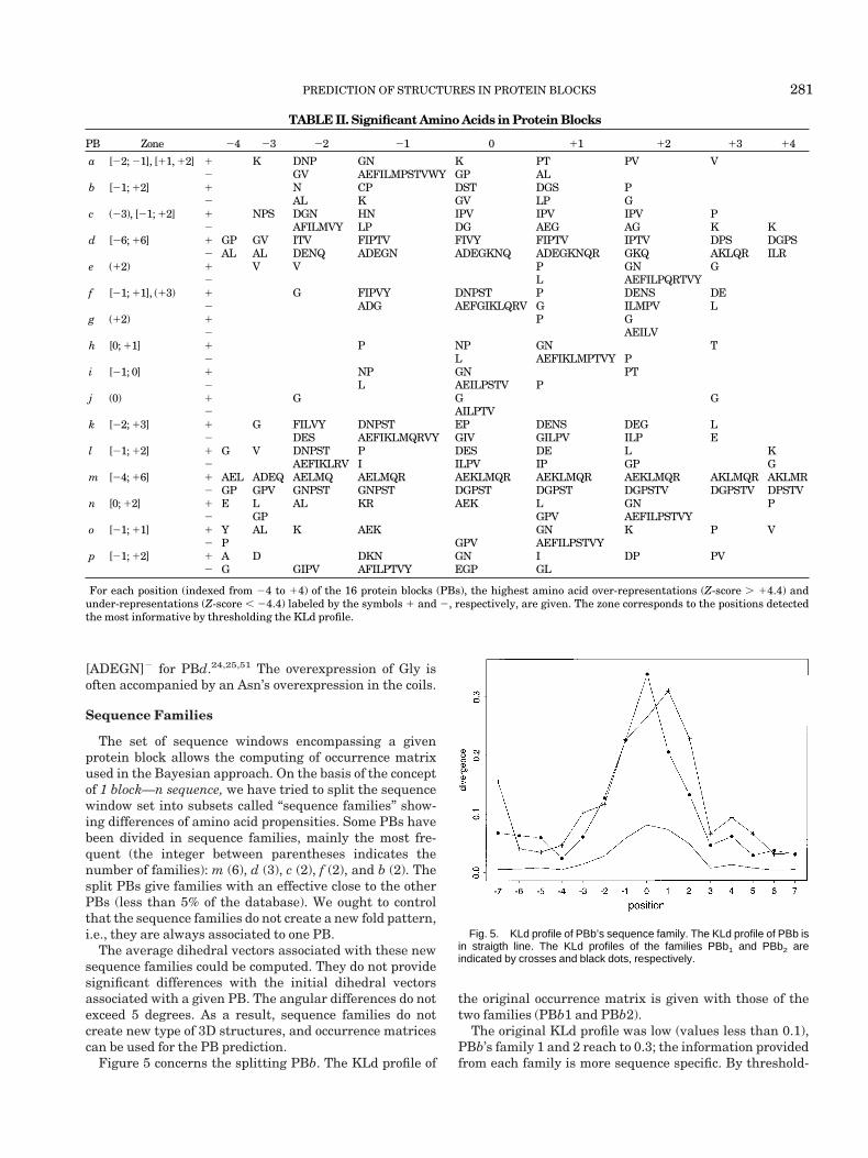
Sequence Families

The set of sequence windows encompassing a givenprotein block allows the computing of occurrence matrixused in the Bayesian approach. On the basis of the conceptof 1 block—n sequence, we have tried to split the sequencewindow set into subsets called “sequence families” show-ing differences of amino acid propensities. Some PBs havebeen divided in sequence families, mainly the most fre-quent (the integer between parentheses indicates thenumber of families): m (6), d (3), c (2), f (2), and b (2). Thesplit PBs give families with an effective close to the otherPBs (less than 5% of the database). We ought to controlthat the sequence families do not create a new fold pattern,i.e., they are always associated to one PB.

The average dihedral vectors associated with these newsequence families could be computed. They do not providesignificant differences with the initial dihedral vectorsassociated with a given PB. The angular differences do notexceed 5 degrees. As a result, sequence families do notcreate new type of 3D structures, and occurrence matricescan be used for the PB prediction.

Figure 5 concerns the splitting PBb. The KLd profile of

the original occurrence matrix is given with those of thetwo families (PBb1 and PBb2).

The original KLd profile was low (values less than 0.1),PBb’s family 1 and 2 reach to 0.3; the information providedfrom each family is more sequence specific. By threshold-

Fig. 5. KLd profile of PBb’s sequence family. The KLd profile of PBb isin straigth line. The KLd profiles of the families PBb1 and PBb2 areindicated by crosses and black dots, respectively.

TABLE II. Significant Amino Acids in Protein Blocks†

PB Zone 24 23 22 21 0 11 12 13 14

a [22; 21], [11, 12] 1 K DNP GN K PT PV V2 GV AEFILMPSTVWY GP AL

b [21; 12] 1 N CP DST DGS P2 AL K GV LP G

c (23), [21; 12] 1 NPS DGN HN IPV IPV IPV P2 AFILMVY LP DG AEG AG K K

d [26; 16] 1 GP GV ITV FIPTV FIVY FIPTV IPTV DPS DGPS2 AL AL DENQ ADEGN ADEGKNQ ADEGKNQR GKQ AKLQR ILR

e (12) 1 V V P GN G2 L AEFILPQRTVY

f [21; 11], (13) 1 G FIPVY DNPST P DENS DE2 ADG AEFGIKLQRV G ILMPV L

g (12) 1 P G2 AEILV

h [0; 11] 1 P NP GN T2 L AEFIKLMPTVY P

i [21; 0] 1 NP GN PT2 L AEILPSTV P

j (0) 1 G G G2 AILPTV

k [22; 13] 1 G FILVY DNPST EP DENS DEG L2 DES AEFIKLMQRVY GIV GILPV ILP E

l [21; 12] 1 G V DNPST P DES DE L K2 AEFIKLRV I ILPV IP GP G

m [24; 16] 1 AEL ADEQ AELMQ AELMQR AEKLMQR AEKLMQR AEKLMQR AKLMQR AKLMR2 GP GPV GNPST GNPST DGPST DGPST DGPSTV DGPSTV DPSTV

n [0; 12] 1 E L AL KR AEK L GN P2 GP GPV AEFILPSTVY

o [21; 11] 1 Y AL K AEK GN K P V2 P GPV AEFILPSTVY

p [21; 12] 1 A D DKN GN I DP PV2 G GIPV AFILPTVY EGP GL

†For each position (indexed from 24 to 14) of the 16 protein blocks (PBs), the highest amino acid over-representations (Z-score . 14.4) andunder-representations (Z-score , 24.4) labeled by the symbols 1 and 2, respectively, are given. The zone corresponds to the positions detectedthe most informative by thresholding the KLd profile.


ing these profiles at a level of 0.08, we observe that PBb1have the most sequence specific positions in the range [23;12], and for positions (27) and (14), and the second in[22; 12]. The KLd profiles are different, the modes are inpositions (11) and (0), respectively.

Comparing the associated occurrence matrices as-sesses the amino acid composition differences: PBb1relative to PBb2 shows an over-representations of Ala inposition (27), Asn (22), Pro (21), His and Asp (0), Pro(11), and Phe (16), and under-representations of Lys(22), Gly (11), and Cys (14). It must be noticed that themain characteristics of the PBb’s occurrence matricesare conserved in the both families, as the overexpressionof Pro in position (12). We point out that the differencesshown correspond to different reallocations of aminoacids. For instance, Ala is over-represented in position(27) in PBb2, although its frequency in PBb1 is same asin the whole database.

Bayesian Prediction of Local StructureProtein block prediction

The prediction is carried out by using the occurrencematrices with the Bayes’ theorem. Here, the under- andover-representations given in Table II play the major rolebecause they determine the quantity Rk for each PB. Rk isthe product of frequencies of the amino acid observed ateach position of the sequence window. Whereas, the “truePB” is geometrically defined by the dihedral vector, the“predicted PB” is simply defined by the rule of the highestRk (or in Rk), this only depends on the sequence windowcentered in a given site of the protein sequence. So, theaccuracy prediction is assessed by comparing the propor-tion of sites where the predicted and the true PBs areidentical. This calculation is performed with the 1

3of the

database not used in the training step. The prediction rateis initially of 30.0% by using the sequence windows of five

amino acids, i.e., the structural window of 5 Ca. The use offlanking sequences (a total window of 15 residues, i.e., asymmetrical elongation of five amino acids encompassingthe structural window) allows a prediction rate of 34.4%(i.e., an gain of 4.4%). The gain is observed for all the PBsand is not specific of the repetitive secondary structure.For example, PBb increases from 11.0% to 13.5%, PBefrom 33.0% to 43.2%, PBi from 32.9% to 42.2%, PBp from26.9% to 33.5%.

Prediction with family sequences

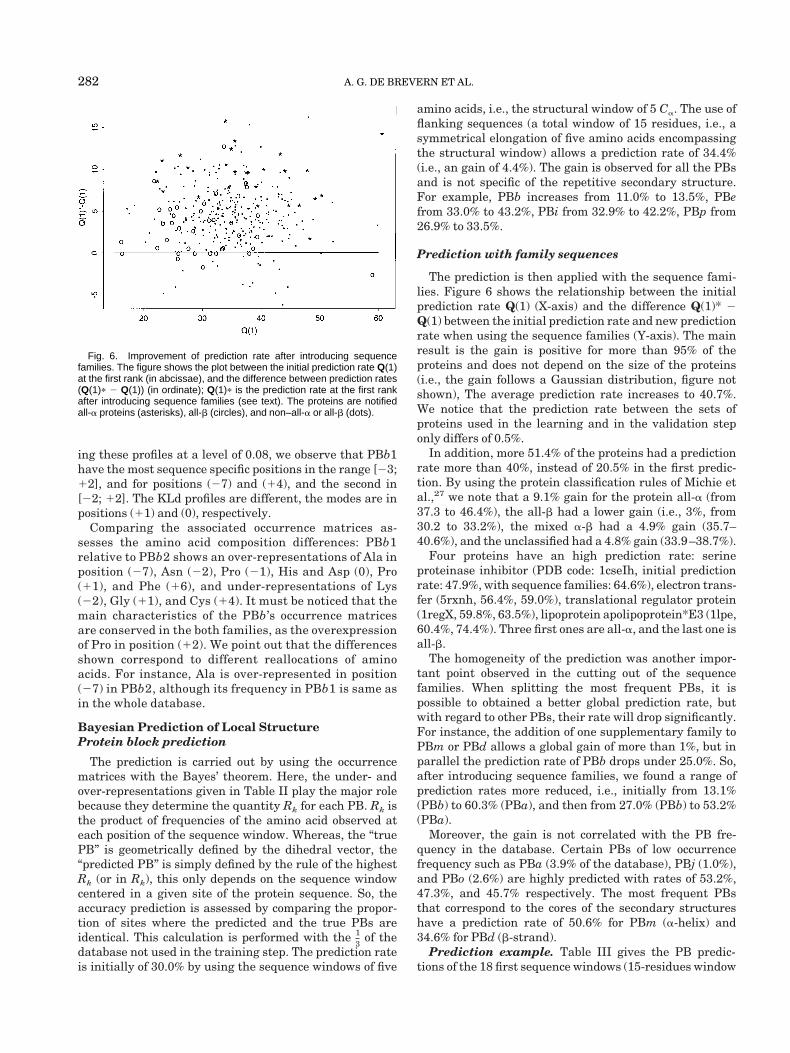
The prediction is then applied with the sequence fami-lies. Figure 6 shows the relationship between the initialprediction rate Q(1) (X-axis) and the difference Q(1)* 2Q(1) between the initial prediction rate and new predictionrate when using the sequence families (Y-axis). The mainresult is the gain is positive for more than 95% of theproteins and does not depend on the size of the proteins(i.e., the gain follows a Gaussian distribution, figure notshown), The average prediction rate increases to 40.7%.We notice that the prediction rate between the sets ofproteins used in the learning and in the validation steponly differs of 0.5%.

In addition, more 51.4% of the proteins had a predictionrate more than 40%, instead of 20.5% in the first predic-tion. By using the protein classification rules of Michie etal.,27 we note that a 9.1% gain for the protein all-a (from37.3 to 46.4%), the all-b had a lower gain (i.e., 3%, from30.2 to 33.2%), the mixed a-b had a 4.9% gain (35.7–40.6%), and the unclassified had a 4.8% gain (33.9–38.7%).

Four proteins have an high prediction rate: serineproteinase inhibitor (PDB code: 1cseIh, initial predictionrate: 47.9%, with sequence families: 64.6%), electron trans-fer (5rxnh, 56.4%, 59.0%), translational regulator protein(1regX, 59.8%, 63.5%), lipoprotein apolipoprotein*E3 (1lpe,60.4%, 74.4%). Three first ones are all-a, and the last one isall-b.

The homogeneity of the prediction was another impor-tant point observed in the cutting out of the sequencefamilies. When splitting the most frequent PBs, it ispossible to obtained a better global prediction rate, butwith regard to other PBs, their rate will drop significantly.For instance, the addition of one supplementary family toPBm or PBd allows a global gain of more than 1%, but inparallel the prediction rate of PBb drops under 25.0%. So,after introducing sequence families, we found a range ofprediction rates more reduced, i.e., initially from 13.1%(PBb) to 60.3% (PBa), and then from 27.0% (PBb) to 53.2%(PBa).

Moreover, the gain is not correlated with the PB fre-quency in the database. Certain PBs of low occurrencefrequency such as PBa (3.9% of the database), PBj (1.0%),and PBo (2.6%) are highly predicted with rates of 53.2%,47.3%, and 45.7% respectively. The most frequent PBsthat correspond to the cores of the secondary structureshave a prediction rate of 50.6% for PBm (a-helix) and34.6% for PBd (b-strand).

Prediction example. Table III gives the PB predic-tions of the 18 first sequence windows (15-residues window

Fig. 6. Improvement of prediction rate after introducing sequencefamilies. The figure shows the plot between the initial prediction rate Q(1)at the first rank (in abcissae), and the difference between prediction rates(Q(1)p 2 Q(1)) (in ordinate); Q(1)p is the prediction rate at the first rankafter introducing sequence families (see text). The proteins are notifiedall-a proteins (asterisks), all-b (circles), and non–all-a or all-b (dots).


encompassing the protein block of 5 Ca) of the protein2aak, ubiquitin conjugating enzyme. A regular a-helix of10 PBm followed by a coil of 7 PBs leading to a b-sheet (seeFig. 3) is studied. This example includes the concept ofsequence families previously described. Each line of thetable corresponding to a sequence window. For instance,the 5th window centered on the motif MRDFK is assignedto PBm. The first three solutions (obtained after orderingthe predictions scores Rk) given by the Bayesian approachare PBm, PBf, and PBb; the respective scores are 22.13,1.25, and 0.40. So, the first score indicates that theprobability of observing the PBm is 22.13 higher than theprobability of observing this block without sequence infor-mation. For this position, the prediction is correct. The twofirst solutions can be explained by taking into account theproportions of amino acids to be located in certain posi-tions of protein blocks (see Table II). The elevated scores ofthe first solutions are justified by the presence of aminoacids Leu, Met, Arg, Lys, Arg, and Leu, respectively, inposition (23), (22), (21), (12), (13), and (14). In the sameway, the block BPf is classified at the second rank becauseof a Asp as central position. By considering the first ranks,10 protein blocks are correctly predicted among the 18 firstblocks. For the whole protein, the prediction rate Q(1)* is40.8%. Without taking into account sequence families, itwas 30.4%, hence, an appreciable gain. Usually, the predic-tion accuracy is only assessed from the solutions of the firstrank. But by observing the solutions given by the threefirst ranks in Table III, we found again 17 of the 18 truePBs. The only misprediction corresponds to an end ofa-helix, which has a unusual amino acid composition inthe central window [24; 14], i.e., KRLQQDPPA. So,rather than only considering the first ranks, an interestingapproach consists of examining the accuracy Q(r) for agiven rank r. The index Neq quantifies the dispersion of

the scores. In the first part of the a-helix, it varies in therange [2.06; 3.78] and it is correlated to an optimalprediction. Reversibly, therefore, the probability of findingthe true BP decreases at the end of the helix, whereas theNeq increases (more than 4.82); this finding reflects thepresence of less informative sites. Moreover, intermediateNeq values are observed for the 7 last residues, the optimalrank is mainly 2. Consequently, a strategy based on amultiple choice of PBs in each site should be informative.

Prediction Strategies

Multiple choices per site. In the database, we observea positive relationship between the highest score (Rk) andthe prediction rate (Q(1)*). We have established that thetrue PB is often among the first selected PBs, i.e., thehighest scores.

The number of selected ranks will be defined by the Neqindex that reflects the dispersion of the 16 scores. Globally,the prediction rate Q(4) for the four first solutions, i.e., thefour PBs with the highest Rk, was 71.4% with the initialBayesian approach, and then by using the family se-quences, it increases to 75.8%. The prediction rates Q(4)*vary according to the PB type from 57.2 (PBg) to 82.8%(PBm). The repetitive PBd and PBm have prediction ratesmore than 80% with this strategy. Therefore, predictionstrategies based on a multiple choice per site should beable to improve the accuracy.

The analysis of the prediction results allows one to pointout that the true PB is generally present among thepredicted PBs showing the highest scores. So two predic-tion strategies can be elaborated: (1) a “global strategy”: todefine the number rs of blocks to be kept in every sites of aprotein to obtain an user-fixed prediction rate Qg, i.e., thetrue protein blocks are found again among the rs selectedPBs with a probability Qg. (2) a “local strategy”: to

TABLE III. Example of Prediction of the 2aak’s N-Terminal†

Sequence

True PB Neq

Predicted PBs

Left c. window Right 1st 2nd 3rd

DMSTP ARKLM RDFKR l 2.74 m(11.21) l(0.63) d(0.36)MSTPA RKLMR DFKRL m 2.43 m(17.51) d(0.74) f(0.43)STPAR KLMRD FKRLQ m 2.06 m(33.68) f(0.38) d(0.18)TPARK LMRDF KRLQQ m 2.63 m(11.05) l(0.51) k(0.36)PARKL MRDFK RLQQD m 2.48 m(22.13) f(1.25) b(0.40)ARKLM RDFKR LQQDP m 3.78 m(7.77) k(1.90) c(0.54)RKLMR DFKRL QQDPP m 2.92 m(12.48) b(0.94) c(0.34)KLMRD FKRLQ QDPPA m 3.49 m(12.98) n(2.60) p(0.73)LMRDF KRLQQ DPPAG m 6.32 m(3.51) n(0.55) d(0.38)MRDFK RLQQD PPAGI m 8.61 p(2.02) b(1.08) m(1.02)RDFKR LQQDP PAGIA m 4.82 p(3.03) d(1.12) c(0.44)DFKRL QQDPP AGIAG c 2.55 c(4.43) d(0.19) p(0.12)FKRLQ QDPPA GIAGA c 3.10 f(13.43) c(2.87) k(0.23)KRLQQ DPPAG IAGAG e 5.45 b(7.14) e(1.94) g(1.68)RLQQD PPAGI AGAGI h 5.34 b(12.39) h(6.72) l(3.16)LQQDP PAGIA GAGIS i 4.97 i(11.29) p(5.29) c(1.40)QQDPP AGIAG AGISG a 4.75 g(15.58) a(6.16) e(3.24)QDPPA GIAGA GISGA c 6.75 b(7.15) h(4.01) c(2.32)†For each window of 15 amino acids, the true protein block (PB), the Neq index, and the three most probable PBs with their own scores Rk aregiven. The underlined PB corresponds to the true one. c. window, center window.


characterize a set of sites for which the user-fixed predic-tion rate Ql is obtained for a fixed number r of PBs.

In the first strategy, the entire protein is predicted interms of protein blocks, but the combination of selectedblocks is variable along the protein. In the second strategy,the protein is restricted to certain sites whose predictionshould be correct with a given probability by taking r PBs.

Global strategy. With the use of the learning data-base, we have established a relationship between theprobability of finding the true PB among the r selectedsolutions and the diversity of score values assessed by Neq(from an entropy assessed from scores normalized intoprobabilities). First, we have selected the blocks for whichthe Neq values vary in a given range. Then the distributionof the rank of the true PB in the solutions has beencalculated. So, for a given prediction rate Qg, we havedetermined from those distributions how many solutions

must be selected for every Neq range (figures not shown).For instance, for a Neq value in the range [1.0; 6.32], weselected the three first PBs given by the Bayesian ap-proach to obtain a 70% prediction rate.

Figure 7 shows the results of this strategy for thestudied protein 2aak. The Neq profile (Fig. 7a) gives thevariation of the index (values between 1.06 at 9.79). Figure7b gives the rank of the true PB in every site of the protein.We note that the true PB is found again in the three firstsolutions for most of the sites (77.8%). Certain restrictedzones of the protein need a higher number of selected PBs,such as the two coils separating the three first b-sheets(positions 22 to 46), and the large coil (positions 82 to 90)containing a small a-helix.

The profile of Figure 7c indicates the number of blocks tobe selected with an average prediction rate Qg of 75%; thetwo dot series below this graph corresponds to the sites

Fig. 7. Protein block (PB) prediction of the ubiquitin conjugatingenzyme (2aak). a: Neq variation along the protein sequence. This indexNeq (“equivalent number of PBs”) based on the Shannon entropyquantifies the prediction uncertainty. b: Rank of the true PB in theprediction. c: Number of selected blocks for an average prediction rate ofQg of 75% with the “global stategy” (see text); the dots show the positionswhere the true PB is found again at the first rank, the smaller ones when itis found among the selected blocks. d: Number of sites selected for a

prediction rate of Ql 5 75% and three PBs per site, with the “local stategy”(see text); the dots indicate the positions where the true PB is found againamong the selected solutions. Forty-nine among 62 selected sites give acorrect prediction. e: Number of sites selected for a prediction rate of Ql 570% and three PBs per site; the dots indicates the positions where thetrue PB is found again among the selected solutions. Ninety-five among122 sites give correct prediction.


where the PB is correctly predicted at the first rank andwhen the true PB is found again in the selected blocks. Themaximum number of PBs is four. The prediction rate isinitially 40.7% with only the first rank; for Qg 5 75%, wekeep 1 to 4 PBs for 8, 17, 37, and 72 sites, respectively. Therepetitive structures and the blocks close to them (cf. Fig.3) are correctly delimited. On the other hand, the coils aremore difficult to be defined. The comparison between thetwo series of points shows that the zones with some truePBs found at the first rank can be spread easier than thezones without true PBs at the first rank.

This strategy leads to an excess of selected blocks in eachposition. However, it selects in every site a number ofblocks so that a given prediction accuracy is ensured.

Local strategy. The second strategy consists of defin-ing limited zones in the protein where the prediction isguaranteed by a number r of selected blocks with a rate Ql.Figure 8 shows the evolution of the prediction rate com-puted function of the Neq index and for different values of r(r varies from 1 to 6). For building these curves, weselected in the whole proteins of the learning database thesites where the Neq index is less than a given value, so thecorresponding proportions of sites are assessed. We thencomputed the proportion of sites in which the true PBs arefound again among the first solution (r 5 1), the two firstsolutions (r 5 2) and so on. So for example, we limit ourprediction to 70% of protein sites; thus, the Neq value mustbe less than 4.8 (see Figure 8). If we only selected one (i.e.,2, 3, and 4) rank(s), we should obtain an average predictionrate of 46.8% (respectively, 63.4%, 73.1%, and 79.6%). Wecould note too for a given prediction rate, for instance 80%,that we will have a Neq index of 1.28 and 5.5% of thepopulation for the first rank (i.e., 1.66 and 11.5% for thesecond rank, 2.61 and 26.9% for the third, 4.64 and 66.3%for the fourth).

Figure 7d indicates for the protein 2aak, the zones forthe prediction rate Ql of 75% and by taking the three first

solutions. The corresponding Neq is less than 5.11. As 62sites had been selected, the dot series indicates the 49positions where a true PB had been found again in theselected positions. So, the observed prediction rate is 79%for 46.3% of the protein positions. By comparison with thefirst approach, it is clear that take three possibilities issometimes an excess. In the same manner, with r 5 4 andQl 5 75% (data not shown), 72 sites (52% of the protein)are concerned.

Figure 7e shows the same strategy with Ql 5 70% andr 5 3 ranks. By taking a Neq maximal of 6.32, 122 sites(91% of the proteins) were selected and 95 sites give thetrue PBs among the three proposed blocks, which corre-sponds to an observed prediction rate of 77.9%.

So, this strategy allows one to locate the sites of highpredictability; however, a critical research must be madein the choice of the number r of ranks to be selected. Forexample, for a prediction accuracy Ql 5 70%, the propor-tion of selected sites in protein rises dramatically with thechange of selection, two into three blocks. This methodproduces a site increase of 49%. In a further application ofthis strategy, in the field of ab initio modeling, the choice ofthe number selected blocks per site raises certain prob-lems such as increasing the rank r leads to a largercovering of the protein, but also to a higher combinatoryvalue between blocks for building a molecular model fromprotein sequence.

DISCUSSION

In our study, we have defined a structural alphabet,which allows the local approximation of the 3D proteinstructure. We have used this library of fragments (PBs) ina new Bayesian probabilistic prediction approach. Wehave then developed two types of strategies, consisting notonly in looking for the most probable block for everyprotein sequence position, but also in searching for theoptimal blocks to be conserved per site with a givenprediction accuracy.

Structural Alphabet

The first important parameter involved in this study isthe length of the PB. Clearly depending on the authors, thelength may be variable or fixed. A constant size is a simpleapproach to perform the prediction step. Long segmentsmust need much more blocks to have the same structuraldescription. Different studies have been carried out usingvarious segment sizes: from 4 to 7 for Rooman et al.,34 from7 to 19 for Bystroff and Baker,20 or fixed at 8 for Unger etal.,32,52 9 for Schuchhardt et al.,33 6 for Fetrow et al.,35 or 4for Camproux et al.36 We have chosen a size of 5 Ca that isconvenient enough to conserve the local contacts withinthe regular structures: positions (i, i 1 2) for the b-strandand (i, i 1 3, i 1 4) for the a-helix.

The second parameter, partially related with the firstone, is the number of PBs. It is critical to learning andprediction steps. Relative to the works of Unger et al.32,52

and Schuchhardt et al.,33 we have determined a limitednumber of small 3D local structures. Our choice is guidedby two facts: (1) the precision of the protein 3D-structure

Fig. 8. Relationship between the Neq index and the prediction rate fordifferent ranks. The prediction rate Q*(r) is assessed according to the Neqvalue (range 5 [1; 8]) or the associated fraction of selected sites in thedatabase. The rank r varies between 1 to 6.


description (expressed into RSMDA), which follows di-rectly from this choice, and (2) the prediction accuracy,which is likewise dependent on this number. In fact,smaller the number of PBs is, more the average RMSDAincreases (i.e., the dihedral angles are less well approxi-mated). Inversely, using a higher number of PBs, forprediction should result in an decreasing prediction accu-racy. To assess the levels of relationship between theparameters, i.e., number of PBs, RMSDA, and Q(1)-value(i.e., prediction accuracy at the first rank), we have carriedout a training allowing a large reduction of PBs by taking ahigh threshold r0 in the structural similarity criterion.With an initial number of 34 PBs and after 8 shrinkingprocesses, we have obtained 10 PBs. The four first shrink-ing show a fast decreasing of the number of PBs with aslow reduction of RMSDA: it dropped from 34 PBs (with anaverage RMSDA of 25.4 degrees) to 22 (28.5 degrees), then19 (29.0 degrees) and 16 (30.0 degrees). The followingprocesses permit one to obtain successively 14, 12, 11, and10 PBs at the end, the angular approximation remainsstable between 30 and 32 degrees in these last steps.

By using a Bayesian prediction without the splittinginto sequence families and only based on a structuralwindow of five amino acids, the accuracy decreases dramati-cally from 34.6 to 30.0% and 22.7% with 10, 16, and 34PBs, respectively. As expected, the prediction accuracy islargely controlled by the number of PBs.

It must be emphasized that for a lower number of PBs(less than 12), the training only yields classic secondarystructures completed by their caps. As the coil regions ofthe protein are more variable than the classic a-helix andb-strand secondary structures, and associated with foldpatterns less frequent, it is necessary to select a highernumber of PBs. Consequently, the choice of 16 BPs isconsistent with a suitable balance between a correctapproximation of the 3D structures (i.e., an averageRMSDA 5 30 degrees) and an acceptable initial predictionaccuracy.

Training Approaches

Different types of methods have been used for classify-ing the 3D segments into a limited set of fold patterns.Various approaches in the field of the training have beenapplied: hierarchical clustering,20,32,34,52 neural net-works,35 self-organized maps (SOM),33 or hidden Markovmodel (HMM).36 Apart the last work, the sequentialdependence between the protein blocks does not take intoaccount as constraints in the training. Another advantageof our unsupervised classifier must be highlighted relativeto the approach HMM37: no hypothesis about the probabil-ity laws of parameters is needed in the model. In fact, it is anonparametric model. Moreover, we have introduced ashrinking process, allowing a fast selection of the optimalnumber of PBs according to a given threshold of structuresimilarity. The algorithm is suited to a fast and efficienttraining of multiple signals (in our study, the dihedralvectors along the proteins). A definition of the proteinblocks partially embedded for ensuring the continuity ofthe protein backbone is of interest in light of its potential

application in the building of molecular models fromprotein sequence.

Prediction and Strategies

The Bayesian probabilistic approach has been fre-quently used.9,38,39 Relative to neural network approach,the scores directly reflect the sequence information con-tent expressed from the amino acid composition in everysite of the sequence window. It is not only limited to a PBsordering. It gives the possibility to compute the Kullback-Leibler asymmetric divergence profiles (i.e., KLd profiles),which point out the most informative amino acid positionsin the sequence window.

Concerning the prediction approach, only rare works inthe literature have been carried out with such a structuralalphabet. Two values for the prediction accuracy areactually available. The first one in the range 65–75%4,5,7 isobtained with a three-states alphabet (classic secondarystructure prediction). The second one is the value given byBystroff and Baker,20 a prediction close to 50% with a13-states alphabet (in reality 13 clusters of fragments ofvarious lengths). It is easy to see that a difference betweena prediction with 3 or 16 blocks cannot give the same levelof accuracy. Bystroff and Baker20 have used a method thatfinally gives 13 clusters of fragments of different length,which are longer than our PBs of 5 Ca; 50% accuracy for a13-states alphabet is close to our results with a 16-statesalphabet.

The developed concept of a fuzzy sequence/3D-structuremodel (1 fold—n sequences/1-sequence—n folds) is reallyimportant in the elaboration of a structural model. Thetwo parts of the fuzzy model have used “1 fold for nsequences” in the definition of the “sequence families” and“1 sequence for n folds” in the both strategies.

The success of the ab initio approach are actually verylimited to only local prediction15 or limited to polypeptidefolds prediction.14 Our approach that leads to a globalprediction solution has to be considered as a very powerfulinitial step coupled with a more elaborated method usingfor instance realistic physical force. Summarizing, twostrategies have been built: the first gives a set of potentialblocks along the sequence. The second one consists ofgiving a constant number of blocks for limited zones. Theonly assumption is that the true PB is among the fewselected ones (this is globally true). It must be noticed asan important point that for each site, the four most likelyPBs are sufficient to provide a high level of prediction rate(more than 75%).

REFERENCES

1. Govindarajan S, Goldstein RA. Why are some proteins structuresso common? Proc Natl Acad Sci USA 1996;93:3341–3345.

2. Govindarajan S, Recabarren R, Goldstein RA. Estimating the totalnumber of protein folds. Proteins 1999;35:408–414.

3. Garnier J, Osguthorpe DJ, Robson B. Analysis of the accuracy andimplications of simple methods for predicting the secondarystructure of globular proteins. J Mol Biol 1978;120:97–120.

4. Garnier J, Gibrat J-F, Robson B. GOR method for predictingprotein secondary structure from amino acid sequence. MethodsEnzymol 1996;266:540–553.

5. Rost B. PHD: predicting one-dimensional protein structure by


profile-based neural networks. Methods Enzymol 1996;266:525–539.

6. Chandonia J-M, Karplus M. The importance of larger data sets forprotein secondary structure prediction with neural networks.Protein Sci 1996;5:768–774.

7. Chandonia J-M, Karplus M. New methods for accurate predictionof protein secondary structure. Proteins 1999;35:293–306.

8. Salamov AA, Solovyev VV. Protein secondary structure predictionusing local alignments. J Mol Biol 1997;268:31–36.

9. Thompson MJ, Goldstein RA. Predicting protein secondary struc-ture with probabilistic schemata of evolutionarily derived informa-tion. Protein Sci 1997;6:1963–1975.

10. Kawabata T, Doi J. Improvement of protein secondary structureprediction using binary word encoding. Proteins 1997;27:36–46.

11. Frishman D, Argos P. The future of protein secondary structureaccuracy. Fold Des 1997;2:159–162.

12. Defay T, Cohen FE. Evaluation of current techniques for ab initioprotein structure prediction. Proteins 1995;23:431–445.

13. Yue K, Dill KA. Folding proteins with a simple energy functionand extensive conformational searching. Protein Sci 1996;5:254–261.

14. Derreumaux P. A diffusion process-controlled Monte Carlo methodfor finding the global energy minimum of a polypeptide chain: I.Formulation and test on a hexapeptide. J Chem Phys 1997;106:5260–5269.

15. Orengo CA, Bray JE, Hubbard T, LoConte L, Sillitoe I. Analysisand assessment of ab initio three-dimensional prediction, second-ary structure, and contacts prediction. Proteins 1999;3(Suppl):149–170.

16. Bowie JU, Luthy R, Eisenberg D. A method to identify proteinsequences that fold into a known three-dimensional structure.Science 1991;253:164–169.

17. Fischer D, Eisenberg D. Protein fold recognition using sequence-derived predictions. Protein Sci 1996;5:947–955.

18. Sali A, Blundell TL. Comparative protein modelling by satisfac-tion of spatial restraints. J Mol Biol 1993;234:779–815.

19. Jaroszewski L, Rychlewski L, Zhang B, Godzik A. Fold predictionby a hierarchy of sequence, threading, and modeling methods.Protein Sci 1998;7:1431–1440.

20. Bystroff C, Baker D. Prediction of local structure in proteins usinga library of sequence-structure motif. J Mol Biol 1998;281:565–577.

21. Simons KT, Ruczinski I, Kooperberg C, Fox BA, Bystroff C, BakerD. Improved recognition of native-like protein structures using acombination of sequence-dependent and sequence-independentfeatures of proteins. Proteins 1999;34:82–95.

22. Simons KT, Bonneau R, Ruczinski I, Baker D. Ab initio proteinstructure prediction of CASP III targets using ROSETTA. Pro-teins 1999;3(Suppl):171–176.

23. Simons KT, Kooperberg C, Huang E, Baker D. Assembly of proteintertiary structures from fragments with similar local sequencesusing simulated annealing and bayesian scoring functions. J MolBiol 1997;268:209–225.

24. Kumar S, Bansal M. Geometrical and sequence characteristics ofa-helices in globular proteins. Biophys J 1998;78:1935–1944.

25. Hutchinson E, Thornton JM. A revised set of potentials for b-turnformation in protein. Protein Sci 1994;3:2207–2216.

26. Orengo CA, Flores TP, Taylor WR, Thornton JM. Identificationand classification of protein fold families. Protein Eng 1993;6:485–500.

27. Michie AD, Orengo CA, Thornton JM. Analysis of domain struc-tural class using an automated class assignement protocol. J MolBiol 1996;262:168–185.

28. Boutonnet NS, Kajava AV, Rooman MJ. Structural classificationof alphabetabeta and betabetaalpha supersecondary structureunits in proteins. Proteins 1998;30:193–212.

29. Wintjens RT, Rooman MJ, Wodak SJ. Automatic classificationand analysis of alpha alpha-turn motifs in proteins. J Mol Biol1996;255:235–253.

30. Kwasigroch J-M, Chomilier J, Mornon J-P. A global taxonomy ofloops in globular proteins. J Mol Biol 1996;259:855–872.

31. Wodjick J, Mornon J-P, Chomilier J. New efficient statisticalsequence-dependent structure prediction of short to medium-sizedprotein loops based on an exhaustive loop classification. J Mol Biol1999;289:1469–1490.

32. Unger R, Harel D, Wherland S, Sussman JL. A 3D building blocksapproach to analyzing and predicting structure of proteins. Pro-teins 1989;5:355–373.

33. Schuchhardt J, Schneider G, Reichelt J, Schomburg D, Wrede P.Local structural motifs of protein backbones are classified byself-organizing neural networks. Protein Eng 1996;9:833–842.

34. Rooman MJ, Rodriguez J, Wodak SJ. Automatic definition ofrecurrent local structure motifs in proteins. J Mol Biol 1990;213:327–336.

35. Fetrow JS, Palumbo MJ, Berg G. Patterns, structures, and aminoacid frequencies in structural building blocks, a protein secondarystructure classification scheme. Proteins 1997;27:249–271.

36. Camproux AC, Tuffery P, Chevrolat J-P, Boisvieux J-F, Hazout S.Hidden Markov Model approach for identifying the modularframework of the protein backbone. Protein Eng 1999;12:1063–1073.

37. Rabiner LR. A tutorial on Hidden Markov Models and selectedapplications in speech recognition. Proc IEEE 1989;77:257–285.

38. Thompson MJ, Goldstein RA. Predicting solvent accessibility:higher accuracy using bayesian statistics and optimized residuesubstitution classes. Proteins 1996;25:38–47.

39. Lathrop RH, Rogers RG Jr, Smith T, White JV. A bayes-optimalsequence-structure theory that unifies protein sequence-structurerecognition and alignement. Bull Math Biol 1998;60:1039–1071.

40. Sternberg MJ, Islam SA. Local protein sequence similarity doesnot imply a structural relationship. Protein Eng 1990;4:125–131.

41. Hobohm U, Scharf M, Schneider R, Sander C. Selection of arepresentative protein data sets. Protein Sci 1992;1:409–417.

42. Hobohm U, Sander C. Enlarged representative set of proteinstructures. Protein Sci 1994;3:522–524.

43. Colloc’h N, Etchebest C, Thoreau E, Henrissat B, Mornon J-P.Comparison of three algorithms for the assignment of secondarystructure in proteins: the advantages of a consensus assignment.Protein Eng 1993;6:377–382.

44. MacArthur MW, Thornton JM. Deviations from planarity ofpeptide bond in peptides and proteins. J Mol Biol 1996;264:1180–1195.

45. Kohonen T. An introduction to neural computing. Neural Net-works 1989;1:3–16.

46. Kohonen T. Self-organizing maps. 2nd ed. Vol. 30. Berlin: Springer-Verlag; 1997. 376 p.

47. Kullback S, Leibler RA. On information and sufficiency. Ann MathStat 1951;22:79–86.

48. Kraulis JP. MOLSCRIPT: a program to produce both detailed andschematic plots of protein structures. J Appl Cryst 1991;24:946–950.

49. Tuffery P. XmMol: an X11 and Motif program for macromolecularvisualization and modelling. J Mol Graph 1995;13:67–72.

50. Richardson JS, Richardson DC. Amino acid preferences for spe-cific locations at the end of a helices. Science 1988;240:1648–1652.

51. Presta LG, Rose GD. Helix signals in proteins. Science 1988;240:1632–1641.

52. Unger R, Sussman JL. The importance of short structural motifsin protein structure analysis. J Comput Aided Mol Des 1993;7:457–472.


bayesian probabilistic approach for predicting...

Documents