Bayesian Non-Local Means Filter,Image Redundancy and Adaptive Dictionaries

for Noise Removal

Charles Kervrann1,3, Jerome Boulanger1,3, and Pierrick Coupe2

1 INRIA, IRISA, Campus de Beaulieu, 35 042 Rennes, France2 Universite de Rennes 1, IRISA, Campus de Beaulieu, 35 042 Rennes, France

3 INRA - MIA, Domaine de Vilvert, 78 352 Jouy-en-Josas, France

Abstract. Partial Differential equations (PDE), wavelets-based methods and neigh-borhood filters were proposed as locally adaptive machines for noise removal.Recently, Buades, Coll and Morel proposed the Non-Local (NL-) means filter forimage denoising. This method replaces a noisy pixel by the weighted average ofother image pixels with weights reflecting the similarity between local neighbor-hoods of the pixel being processed and the other pixels. The NL-means filter wasproposed as an intuitive neighborhood filter but theoretical connections to dif-fusion and non-parametric estimation approaches are also given by the authors.In this paper we propose another bridge, and show that the NL-means filter alsoemerges from the Bayesian approach with new arguments. Based on this obser-vation, we show how the performance of this filter can be significantly improvedby introducing adaptive local dictionaries and a new statistical distance measureto compare patches. The new Bayesian NL-means filter is better parametrizedand the amount of smoothing is directly determined by the noise variance (esti-mated from image data) given the patch size. Experimental results are given forreal images with artificial Gaussian noise added, and for images with real image-dependent noise.

1 Introduction

Denoising (or restoration) is still a widely studied and an unsolved problem in imageprocessing. Many methods have been suggested in the literature, and a recent outstand-ing review of them can be found in [4]. Some of the more advanced methods are basedon PDEs [28, 29, 33, 37] and aim at preserving the image details and local geometrieswhile removing the undesirable noise; in general, an initial image is progressively ap-proximated by filtered versions which are smoother or simpler in some sense. Othermethods incorporate a neighborhood of the pixel under consideration and perform somekind of averaging on the gray values. One of the earliest examples for such filters hasbeen presented by Lee [23] and a recent evolution is the so-called bilateral filter [34]with theoretical connections to local mode filtering [38], non-linear diffusion [3, 5] andnonlocal regularization approaches [27, 12].

However, natural images often contain many structured patterns which can be mis-classified either as details to be preserved or noise, when usual neighborhood filtersare applied. Very recently, the so-called NL-means filter has been proposed by Buades

et al. [4] that can deal with such a “structured” noise: for a given pixel, the restoredgray value is obtained by the weighted average of the gray values of all pixels in theimage; each weight is proportional to the similarity between the local neighborhoodof the pixel being processed and the neighborhood corresponding to the other imagepixels. A similar patch-based regularization approach based on the key idea of itera-tively increasing a window at each pixel and adaptively weighting input data has beenalso proposed in [21] with excellent results on a commonly-used image database [31].The success of the NL-means filter (see [21, 22, 26, 25, 7, 16, 2]), inspired by the Efrosand Leung’s exemplar-based approach for texture synthesis [11], is mainly related toimage redundancy. A similar idea was early and independently proposed for Gaussian[9] and impulse noise [36, 39] removal in images, and more recently for image inpaint-ing [8]. Similarities between image patches have been also used in the early 90’s fortexture segmentation [15, 20]. More recently, other recent denoising methods demon-strated that representations based on local image patches outperform the best denoisingmethods of the state-of-the-art [1, 21, 10, 18, 13]; in [32], patch-based Markov randomfield (MRF) models and learning techniques have been introduced to capture non-localpairwise interactions, and were successfully applied in image denoising.

In this paper, we present a new Bayesian motivation for the NL-means filter brieflydescribed in Section 2. In Section 3, we adopt a blockwise (vectorial) representation andintroduce spatially adaptive dictionaries in the modeling for better contrast restoration(Section 4). Using the proposed Bayesian framework, we revise the usual Euclideandistance used for patch comparison, yielding to a filter which is better parametrized,and with a higher performance. In Section 4, we also show how smooth parts in the im-age can be are better recovered if the restored image is “recycled” once. Experimentalresults on artificial and real images are presented in Section 5, and the performance isvery close to the most competitive denoising methods. It is worth noting that the pro-posed modeling framework is general and could be used to restore images corruptedby non-Gaussian noises in applications such as biomedical imaging (microscopy, ultra-sound imagery, ...) or remote sensing.

2 Image denoising with the NL-means filter

In this section, a brief overview of the NL-means method introduced in [4] is presented.Consider a gray-scale image z = (z(x))x∈Ω defined over a bounded domain Ω ⊂ R

2,(which is usually a rectangle) and z(x) ∈ R+ is the noisy observed intensity at pixelx ∈ Ω. The NL-means filter is defined as

NL z(x) =1

C(x)

∑

y∈Ω

w(x, y) z(y) (1)

where NL z(x) at pixel x is the weighted average of all gray values in the image andC(x) is a normalizing factor, i.e. C(x) =

∑y∈Ω w(x, y). The weights w(x, y) defined

as

w(x, y) = exp

(− 1

h2

∫

R2

Ga(t)|z(x + t)−z(y + t)|2dt

):=exp−‖z(x)−z(y)‖2

2,a

h2(2)

express the amount of similarity between the vectorized image patches z(x) and z(y)(or neighborhoods) of each pair of pixels x and y involved in the computation. Thedecay parameter h ≈ 12σ acts as a filtering parameter. A Gaussian kernel Ga(·) ofstandard deviation a is used to take into account the distance between the central pixeland other pixels in the patch. In (2), the pixel intensities of a

√n × √

n square neigh-borhood B(x) centered at pixel x, are taken and reordered lexicographically to forma n-dimensional vector z(x) := (z(xk), xk ∈ B(x)) ∈ R

n. In [4], it was shown that7×7 patches are able to take care of the local geometries and textures seen in the imagewhile removing undesirable distortions. The range of the search space in the NL-meansalgorithm can be as large as the whole image. In practice, it is necessary to reduce thetotal number of computed weights – |Ω| weights for each pixel – to improve the per-formance of the algorithm. This can be achieved by selecting patches in a semi-localneighborhood corresponding to a search window ∆(x) of 21×21 pixels. The NL-meansfilter we will now consider, is then defined as

NLhz(x) =1

C(x)

∑

y∈∆(x)

e−‖z(x)−z(y)‖2/h2

z(y), C(x) =∑

y∈∆(x)

e−‖z(x)−z(y)‖2/h2

(3)

where, for the sake of simplicity, ‖ · ‖ denotes the usual `2-norm. In practice, it isjust required to set the

√n × √

n patch size, the search space ∆(x) and the filteringparameter h. Buades et al. showed that this filter substantially outperforms the bilateralfilter [34] and other iterative approaches [33].

Since, several accelerated versions of this filter have been proposed [26, 7]. In [4],Buades et al. recommended the vectorial (or block-based) NL-means filter defined as

NLhz(x) =1

C(x)

∑

y∈∆(x)

e−‖z(x)−z(y)‖2/h2

z(y), C(x) =∑

y∈∆(x)

e−‖z(x)−z(y)‖2/h2

, (4)

which amounts to simultaneously restore pixels of a whole patch z(x) from nearbypatches. The restored value at a pixel x is finally obtained by averaging the differ-ent estimators available at that position [4]. This filter can been considered as a fastimplementation of the NL-means filter, especially if the blocks are picked up on a sub-sampled grid of pixels. In this paper, the proposed filter is inspired by this intuitivevectorial NL-means filter [4], but also by other recent accelerated versions [26, 7], asexplained in the next sections. The related Bayesian framework enables to establish therelationships between these algorithms, to justify some underlying statistical assump-tions and to give keys to set the control parameters of the NL-means filter. It is worthnoting that this framework could be also used to remove noise in applications for whichthe noise distribution is assumed to be known and non-Gaussian.

3 A Bayesian risk formulation

In a probabilistic setting, the image denoising problem is usually solved in a discretesetting. The estimation problem is then to guess a n-dimensional patch u(x) from itsnoisy version z(x) observed at point x. Typically, the unknown vectorized image patch

u(x) is defined as u(x) := (u(xk), xk ∈ B(x)) ∈ Rn where B(x) defines the

√n×√

nsquare neighborhood of point x and the pixels in u(x) are ordered lexicographically.Let us suppose now that u(x) is unknown but we can observe z(x) = f(u(x),v(x))where z(x) := (z(xk), xk ∈ B(x)), v(x) represents noise and f(·) is a linear or anon-linear function related to the image formation process. The noise v(x) is a randomvector which components are iid, and u(x) is considered as a stochastic vector withsome unknown probability distribution function (pdf).

Conditional mean estimator To compute the optimal Bayesian estimator for the vec-tor u(x), it is necessary to define an appropriate loss function L(u(x), u(x)) whichmeasures the loss associated with choosing an estimator u(x) when the true vector isu(x). The optimal estimator uopt(x) is found by minimizing the posterior expected loss

E[L(u(x), u(x))] =∑

u(x)∈Λ

L(u(x), u(x)) p(u(x)|z(x)),

taken with respect to the posterior distribution p(u(x)|z(x)) and Λ denotes the largespace of all configurations of u(x) (e.g |Λ| = 256n if u(x) ∈ 0, · · · , 255). Theloss function used in most cases is L(u(x), u(x)) = 1 − δ(u(x), u(x)) where the δfunction equals 1 if u(x) = u(x) and 0 otherwise. Minimizing E[L(u(x), u(x))] isthen equivalent to choose uopt(x) = argmax p(u(x)|z(x)), with the motivation thatthis should correspond to the most likely vector given the observation z(x). However,this loss function L(u(x), u(x)) may not be the most appropriate since it assigns 0 costonly to the perfect solution and unit cost to all other estimators. Another thought wouldbe to use a cost function that depends on the number of pixels that are in error such asL(u(x), u(x)) = ‖u(x) − u(x)‖2. Assuming this quadratic loss function, the optimalBayesian estimator is then

uopt(x) = arg minbu(x)

∑

u(x)

‖u(x) − u(x)‖2 p(u(x)|z(x)) =∑

u(x)

u(x) p(u(x)|z(x)).

Referred as the conditional mean estimator, uopt(x) can be also written as

uopt(x) =∑

u(x)

u(x)p(u(x), z(x))

p(z(x))=

∑u(x) u(x)p(z(x)|u(x))p(u(x))∑

u(x) p(z(x)|u(x))p(u(x))(5)

by using the Bayes’ and marginalization rules, and p(z(x)|u(x)) and p(u(x)) respec-tively denote the distribution of z(x)|u(x) and the prior distribution of u(x).

Bayesian filter and image redundancy Ideally, we would like to know the pdfsp(z(x)|u(x)) and p(u(x)) to compute uopt(x) for each point x in the image from alarge number of “repeated” observations (i.e. images). Unfortunately, we have only oneimage at our disposal, meaning that we have to adopt another way of estimating thesepdfs. Due to the fact that the pdfs p(z(x)|u(x)) and p(u(x)) cannot be obtained froma number of observations at the same point x, we choose to use the observations at anumber of neighboring points taken in a semi-local neighborhood (or window) ∆(x).The window ∆(x) needs to be not too large since the remote samples are likely less

significant and can originate from other spatial contexts. We then assume that this setof nearby samples may be considered as a set of samples from p(u(x)|z(x)).

More formally, we suppose that p(u(x)|z(x)) is unknown, but we have a set u(x1),u(x2), · · · ,u(xN(x)) of N(x) posterior samples taken in ∆(x). In what follows,|∆(x)| is fixed for all the pixels but the size N(x) ≤ |∆(x)| is spatially varying sinceirrelevant and unlikely samples in ∆(x) are preliminarily discarded. From this set, westart by examining the prior distribution p(u(x)). A first natural ideal would be to intro-duce MRFs and Gibbs distributions to capture interactions between pixels in the imagepatch, but the MRF framework involves the computationally intensive estimation of ad-ditional hyperparameters which must be likely adapted to each spatial position. Dueto the huge domain space Λ, a computational alternative is then to set p(u(x)) to uni-form, i.e. p(u(x)) = 1/N(x). This means there is no preference to choose a vectoru(xi) in the set u(x1), · · · ,u(xN(x)) assumed to be composed of N(x) preliminar-ily selected “similar” patches. Then, we have the following approximations (see [17]):

1

N(xi)

N(xi)X

j=1

u(xj)p(z(xi)|u(xj))P→

X

u(x)

u(x)p(z(x)|u(x))p(u(x)),

1

N(xi)

N(xi)X

j=1

p(z(xi)|u(xj))P→

X

u(x)

p(z(x)|u(x))p(u(x)),

and we can propose a reasonable estimator uN (xi) for uopt(x):

uN (xi) =

1N(xi)

∑N(xi)j=1 u(xj)p(z(xi)|u(xj))

1N(xi)

∑N(xi)j=1 p(z(xi)|u(xj))

. (6)

Nevertheless, we do not have the set u(x1), · · · ,u(xN(x)), but only a spatially vary-ing dictionary D(x) = z(x1), · · · , z(xN(x)) composed of noisy versions is available.A way to solve this problem will be then to substitute z(xj) to u(xj) in (6) as shown inthe next section. In a second step, this estimator will be refined by substituting the “ag-gregated” estimator computed from uN (xj) (see below) to u(xj). Indeed, the restoredpatch at pixel xj is a better approximation of u(xj) than the noisy patch z(xj) used asa “pilot” estimator, and the performance will be improved at the second iteration.

Aggregation of estimators The estimator (6) requires spatially sliding windows overthe whole image for image reconstruction. Hence, a set of L (constant for uniform im-age sub-sampling) concurrent scalar values uN,1(xi), uN,2(xi), · · · , uN,L(xi) is calcu-lated for the same pixel xi due to the overlapping between patches. This set of compet-ing estimators must be fused or aggregated into the one final estimator u(xi) at pixel xi.Actually, when no estimator is a “clear winner”, one may prefer to combine the differentestimators uN,1(xi), uN,2(xi), · · · , uN,L(xi) and a natural approach, well-grounded instatistics [6], is to use a convex or linear combination of estimators [19, 10]. Here, ouraggregate estimator uN (xi) is simply defined as the average of competing estimators:

uN(xi) =1

L

L∑

l=1

uN,l(xi). (7)

In practice, patches are picked up on a sub-sampled grid (e.g. factor 3) of pixels to speedup the algorithmic procedure (e.g. factor 8), while preserving a good visual quality.

4 Bayesian NL-means filter

As explained before, to compute uN (xi), we first substitute z(x) to u(x) in (6). Thisyields the following estimator

1N(xi)

∑N(xi)j=1 p(z(xi)|z(xj))z(xj )

1N(xi)

∑N(xi)j=1 p(z(xi)|z(xj ))

≈ uN (xi) (8)

which can be computationally calculated provided the pdfs are known. It is worth notingthat p(z(xi)|z(xj)) is not well defined if xi = xj and it could be recommended to setp(z(xi)|u(xi)) ≈ maxxj 6=xi

p(z(xi)|z(xj)) in (8) (see [22]). The central data pointinvolved in the computation of its own average is then re-weighted to get the higherweight. Actually, the probability to detect an exact copy of z(xi) corrupted by noise inthe neighborhood tends to 0 because the space of

√n ×√

n patches is huge and, to beconsistent, it is necessary to limit the influence of the central patch.

In the remainder of this section, we shall now consider the usual image model

z(x) = u(x) + v(x) (9)

where v(x) is an additive white Gaussian noise with variance σ2. We will further as-sume that the likelihood can be factorized as p(z(xi)|z(xj )) =

∏nk=1 p(z(xi,k)|z(xj,k))

with xi,k ∈ B(xi) and xj,k ∈ B(xj). It follows that z(xi)|z(xj) follows a multivari-ate normal distribution, z(xi)|z(xj ) ∼ N (z(xj ), σ

2In) where In is the n-dimensional

identity matrix. From (8), the filter adapted to white Gaussian noise is then given by

1

C(xi)

N(xi)∑

j=1

e−‖z(xi)−z(xj)‖2/(2σ2)z(xj) with C(xi) =

N(xi)∑

j=1

e−‖z(xi)−z(xj)‖2/(2σ2).(10)

If we arbitrarily set N(xi) = N to a constant value and h2 = 2σ2, this filter is nothingelse than the vectorial NL-means filter given in (4). However, it is recommended to seth ≈ 12σ in [4] to produce satisfying denoising results. In our experiments, it is alsoconfirmed that h ≈ 5σ is good choice if we use (3) and (4) for denoising. Actually, thefiltering parameter h is actually set to a higher value than the expected value

√2σ in

practical imaging. In the next sections, we shall see how this parameter can be betterinterpreted and theoretically estimated.

Spatially adaptive dictionaries The filter (10) can be refined if the adaptive dictio-nary D(xi) = z(x1), · · · , z(xN(xi)) around xi is reliably obtained using an off-lineprocedure. Since D(xi) is assumed to be composed of noisy versions of the more likelysamples from the posterior distribution p(u(xi)|z(xi)), the irrelevant image patches in∆(xi) must be discarded in a preliminary step. Consequently, the size N(xi) is adaptiveaccording to local spatial contexts and a simple way to detect these unwanted samplescan be based on local statistical features between images patches. In our experiments,we have consider two basic features, that is the mean m(z(x)) = n−1

∑nk=1 z(xk)

and the variance var(z(x)) = n−1∑n

k=1(z(xk) − m(z(x)))2 of a vectorized patchz(x) := (z(xk), xk ∈ B(x)).

Intuitively, z(xj) will be discarded from the local dictionary D(xi) if the meanm(z(xj)) is too ‘far” from the mean m(z(xi)) when z(xj) and z(xi) are compared.More formally, if |m(z(xj )) − m(z(xi))| > λασ/

√n, where λα ∈ R+ is chosen as a

quantile of the standard normal distribution, the hypothesis that the two patches belongto the same “population” is rejected. Hence, setting λα = 3 given P(|m(z(xj )) −m(z(xi))| ≤ λασ/

√n) = 1 − α, yields to α = 2(1 − Φ(λα/

√2)) = 0.034 where Φ

means the Laplace distribution.Similarly, the variance var(z(xj )) is expected to be close to the variance var(z(xi))

for the central patch z(xi). A F -test4 is used and the ratio F =max(var(z(xj)),var(z(xi)))min(var(z(xj)),var(z(xi)))

is compared to a threshold Tβ,n−1 to determine if the value falls within the zone ofacceptance of the hypothesis that the variances are equal. The threshold Tβ,n−1 is thecritical value for the F -distribution with n − 1 degrees of freedom for each patch anda significance level β. Typically, when 7 × 7 patches are compared, we have P(F >T0.05,48 = 1.6) = 0.05. If the ratio F exceeds the value Tβ,n−1, the sample z(xj) isdiscarded from the local dictionary D(xi).

This formal description is related to the intuitive approach proposed in [26, 7, 16] toimprove the performance of the NL-means filter.

New statistical distance measure for patch comparison In this section, we pro-pose to revise the distance used for patch comparison, yielding to a NL-means filterwhich is better parametrized. In (3) and (4), it is implicitly assumed that z(xi)|z(xj) ∼N (z(xj ),

12h2

In). Actually, this hypothesis is valid only for non-overlapping and sta-tistically independent patches, but most of patches overlapped in ∆(x) since ∆(x) isnot so large (e.g 21× 21 pixels). At the opposite, if z(xj) is horizontally (or vertically)shifted by one pixel from the location of z(xj ), z(xi)|z(xj ) is expected to follow amultivariate Laplacian distribution. However, this statistical hypothesis does not holdtrue for arbitrary locations of overlapping patches in ∆(x). The adjustment of the de-cay parameter h ≈ 5σ in (3) to a value higher that the expected value

√2σ is probably

related to the fact that the two compared patches are not independent. Note that somepixel values are in common in the two vectors but at different locations.

Hence, p(z(xi)|z(xj)) must be carefully examined and we propose the followingdefinition for the likelihood: p(z(xi)|z(xj )) ∝ e−φ(‖z(xi)−z(xj)‖). Typically, we canchoose φ(t) = t2 or φ(t) = |t| (or a scaled version) to compare patches. Here, weexamine the distribution of ‖z(xi) − z(xj)‖ from the local dictionary D(xi) to deter-mine φ. First, it can be observed that E[‖z(xi)− z(xj)‖] is non-zero in most cases andthe probability to find an exact copy of z(xi) in ∆(x) tends to 0, especially if ∆(x) islarge. The maximum of the assumed zero-mean multivariate Gaussian distribution in (3)should be then “shifted” to E[‖z(xi)−z(xj)‖]. However, this training step could be hardin practice since it must adapted to each spatial position, and we propose instead to useasymptotic results. Actually, we have already assumed (z(xi,k)−z(xj,k)) ∼ N (0, 2σ2)when two pixels taken in z(xi) and z(xj) ∈ D(xi) are compared. Hence, the normal-ized distance dist(z(xi), z(xj)) = ‖z(xi) − z(xj )‖2/(2σ2) follows a chi-square χ2

n

distribution with n degrees of freedom. For n large (n ≥ 25), it can be proved that√2 dist(z(xi), z(xj )) is approximately normally distributed with mean

√2n − 1 and

4 The F -distribution is used to compare the variance of two independent samples from a normally distributed population.

unit variance:

p(√

2 dist(z(xi), z(xj))∝ exp−1

2

(√2 dist(z(xi), z(xj)) −

√2n − 1

)2

(11)

∝ exp−(‖z(xi) − z(xj )‖2

2σ2− ‖z(xi) − z(xj)‖

(σ/√

2n − 1)+

2n− 1

2

).

Accordingly, we define the likelihood as p(z(xi)|z(xj )) ∝ exp−φ(‖z(xi) − z(xj)‖)and choose φ(t) = at2 − b|t| + c with a = 1/(2σ2), b =

√2n − 1/σ and c =

(2n − 1)/2 depending only on the patch size n and the noise variance σ2. From ourexperiments, it was confirmed that no additional adjustment parameter is necessaryprovided the noise variance is robustly estimated and the performance is maximum forthe true noise variance as expected. Figure 1 (bottom-right) shows the functions e−t2/h2

and e−(|t|/σ−√

2n−1)2/2 by setting n = 49, σ2 = 1 and h = 5σ, and then illustrates howdata points are currently weighted when the original NL-means filter and the so-calledAdaptive NL-means filter (ANL) defined as

ANLσ,nz(xi) =

N(xi)∑

j=1

exp−1

2

(‖z(xi) − z(xj)‖σ

−√

2n − 1

)2

z(xj)

N(xi)∑

j=1

exp−1

2

(‖z(xi) − z(xj)‖σ

−√

2n − 1

)2. (12)

where N(xi) = #D(xi), are applied. Note that the data at point xi should partic-ipate significantly to the weighted average. Accordingly, since p(z(xi)|z(xj )) tends to 0when xi = xj in (12), we arbitrarily decide to set p(z(xi)|z(xi)) ≈ maxxj 6=xi

p(z(xi)|z(xj))as explained before (see also [22]).

Bayesian NL-means filter and plugin estimator In the previous sections, z(xj) wassubstituted to u(xj) in (6) to give (8) and further (12). Now, we are free to substitutethe vector uANL(xj) of aggregated estimators (computed from the set of restored blocksANLσ,nz(xj) , see (7)) to u(xj). This plugin ANL estimator defined as

ANLσ,nuANL(xi) =

N(xi)∑

j=1

exp−1

2

(2 ‖z(xi) − uANL(xj)‖

σ−√

2n − 1

)2

uANL(xj)

N(xi)∑

j=1

exp−1

2

(2 ‖z(xi) − uANL(xj)‖

σ−√

2n − 1

)2(13)

is expected to improve the restored image since uANL(xj) is a better approximationof u(xj) than z(xj). In (13) the restored image is recycled but the weights is a re-scaled function (theoretically by a factor 2) of the distance between the “pilot” esti-mator uANL(xj) given by (12) and the input vector z(xi). The estimators are finallyaggregated to produce the final restored image (see (7)).

5 Experiments

In this section, we evaluate the performance of different versions of the Bayesian fil-ter and the original NL-means filter using the peak signal-to-noise ratio (PSNR in db)defined as PSNR = 10 log10(2552/MSE) with MSE = |Ω|−1

∑x∈Ω(z0(x) − u(x))2

where z0 is the noise-free original image. We also use the “method noise” describedin [4] which consists in computing the difference between the input noisy image andits denoised version. The NL-means filter (see (3)) was applied with h = 5σ and ourexperiments have been performed with 7 × 7 patches and 15 × 15 search windows,corresponding to the best visual results and the best PSNR values. For all the presentedresults, we set T0.05,n−1 = 1.6 and λ0.034 = 3 to build spatially adaptive dictionaries.

The potential of the estimation method is mainly illustrated with the 512×512 Lenaand Barbara images corrupted by an additive white-Gaussian noise (WGN) (PSNR =22.13 db, σ = 20). We compared the original NL-means algorithm with the proposedmodifications and Fig. 1 shows the denoising results using several filters (n = 7×7 andN = 15×15): i) the NL-means filter NLhz when the similarity is only measured by theEuclidean distance (see (3)); ii) the vectorial NL-means filter NLhz with sliding blocksbut no spatial sub-sampling (see (4)); iii) our Adaptive NL-means filter ANLσ,nz whichincludes adaptive dictionaries and a similarity measure based on the new distance (see(12)); iv) the plugin Adaptive NL-means filter ANLσ,nuANL (see (13)). In most cases,the PSNR values are slightly affected if a spatial sub-sampling (by a factor 3) is usedin the implementation, but the time computing is drastically reduced (speed is 8 timesless than before): the implementation of the fast Adaptive NL-means filter took 10 secon a single-CPU PC 2.0 Ghz running linux, and the full Adaptive NL-means filter (withno spatial sub-sampling) took 75 sec for denoising a 512 × 512 image (see table inFig. 1). In these practical examples, the use of spatially adaptive dictionaries enablesto enhance contrasts. Note that the residual noise in flat zones is more reduced withno additional blur, when ANLσ,nuANL is applied. In Fig. 2, we modified the estima-tion of noise variance to assess the sensitivity of this parameter on filtering results. Ingeneral, the PSNR value is maximum with the true value (e.g. σ = 20 in Fig. 2) butdecreases if this value is under-estimated or over-estimated. In Fig. 2, the estimatednoise component is similar to a simulated white Gaussian noise but contains few geo-metric structures if we under-estimate or over-estimate the noise variance. To evaluatethe performance of those filters, we reported the PSNR values for different versions ofthe NL-means filter. In table 1, the numerical results are improved using our filter, withperformance very close to competitive patch-based denoising methods. Note that thebest results (PSNR values) were recently obtained by filtering in 3D transform domainand combining sliding-window transform processing with block-matching [10].

In the second part of experiments, we have applied ANLσ,nuANL to restore an oldphotograph (Fig. 3 - left column); in that case, the noise variance is estimated from im-age data (see [21]). Nevertheless, in real digital imaging, images are better described bythe following model z(x) = u(x)+uγ(x) ε(x) where the sensor noise uγ(x) ε(x) is de-fined as a function of u(x) and ε(x) is a zero-mean Gaussian noise of variance σ2. Ac-cordingly, the noise in bright regions is higher than in dark regions (see Fig. 2 - secondcolumn). From experiments on real digital images [14], it was confirmed that γ ≈ 0.5(γ = 0 corresponds to WGN in the previous experiments). Accordingly, we modify the

noisy image (σ = 20) NLhz NLhz ANLσ,nz ANLσ,neuANL

Timings Lena Barbara512 × 512 512 × 512

NLhz 58.1 sec 31.85 db 30.27 dbNLhz 96.2 sec 32.04 db 30.49 dbANLσ,nz 75.2 sec 32.51 db 30.79 dbANLσ,neuANL 173.3 sec 32.63 db 30.88 dbFast ANLσ,nz 10.6 sec 32.36 db 30.61 dbFast ANLσ,neuANL 21.2 sec 32.49 db 30.71 db

−10 −5 0 5 10 150

0.05

0.1

0.15

0.2

0.25

0.3

0.35

0.4

Fig. 1. Comparisons of different NL-means filters. From top to bottom and from left to right: part of noisy images (Barbara,Lena, σ = 20), NL-means filter, vectorial NL-means filter, Adaptive NL-means filter, plugin Adaptive NL-means filter;numerical results for each filter; comparison of exponential weights for the original NL-means filter (blue dashed line) andfor the Adaptive NL-means filter (solid green line) (see text).

normalized distance as follows: dist(z(xi), z(xj)) = ‖z(xi) − z(xj)‖2/(2σ2z(xj))

with σ ∈ [1.5, 3]. Moreover, this model z(x) = u(x) +√

u(x) ε(x) has already beenconsidered to denoise log-compressed ultrasonic images [24]. Preliminary results ofANLσ,nuANL with this model is shown in Fig. 3, when applied to two log-compressedultrasonic images and a cryo-Electronic Microscopy image (cross-section of a micro-tubule (10-30 nm)) where brights areas are smoother than dark areas.

6 Conclusion

We have described a Bayesian motivation for the NL-means filter and justify some intu-itive adaptations described in previous papers [4, 26, 7]. The proposed framework yieldsto a filter which is better parametrized: the size of the adaptive dictionary and the noisevariance are computed from the input image, and the patch size must be large enough.Our Bayesian approach has been used to remove image-dependent noise and could beadapted in applications with appropriate noise distributions. A more thoroughly evalu-ation with other methods [1, 2, 35, 16], and recent improvements of the NL-means filterdescribed in [5], would be also desirable.

Acknowledgments. We thank B. Delyon and P. Perez for fruitful conversations and comments.

σ = 15 σ = 18 σ = 20 σ = 22 σ = 25PSNR = 28.91 db PSNR = 32.03 db PSNR = 32.63 db PSNR = 32.29 db PSNR = 31.29 db

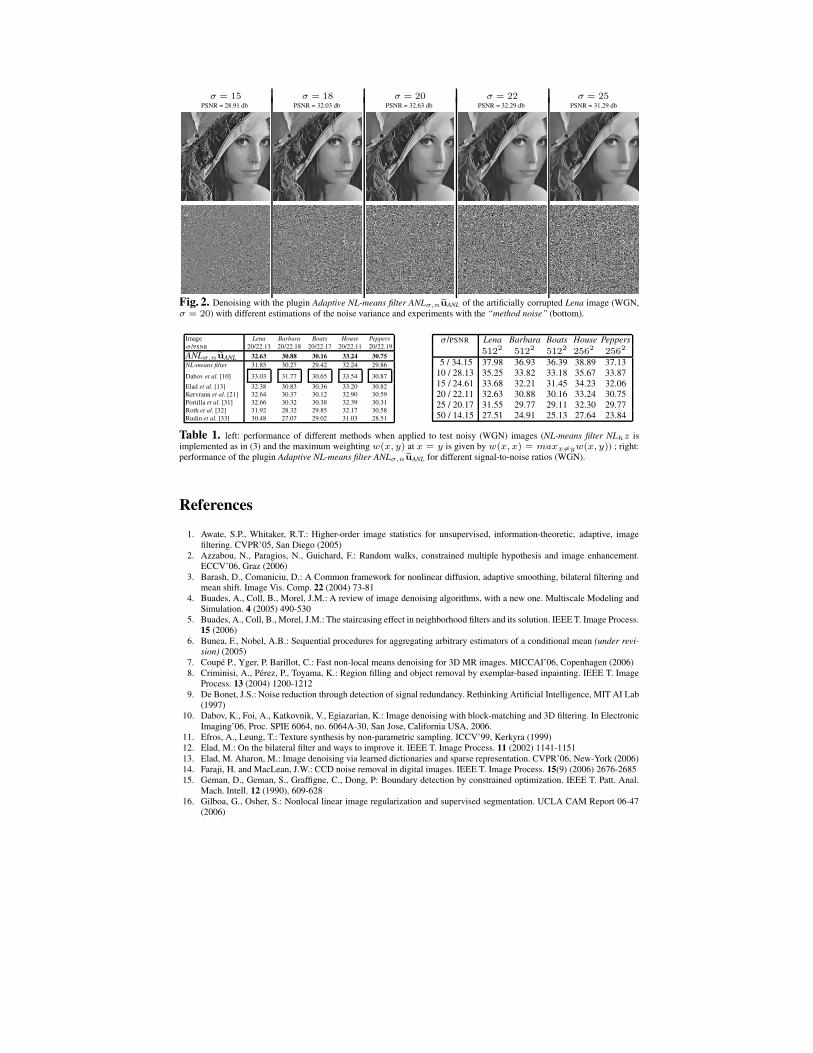
Fig. 2. Denoising with the plugin Adaptive NL-means filter ANLσ,neuANL of the artificially corrupted Lena image (WGN,σ = 20) with different estimations of the noise variance and experiments with the “method noise” (bottom).

Image Lena Barbara Boats House Peppersσ/PSNR 20/22.13 20/22.18 20/22.17 20/22.11 20/22.19ANLσ,neuANL 32.63 30.88 30.16 33.24 30.75NL-means filter 31.85 30.27 29.42 32.24 29.86

Dabov et al. [10] 33.03 31.77 30.65 33.54 30.87

Elad et al. [13] 32.38 30.83 30.36 33.20 30.82Kervrann et al. [21] 32.64 30.37 30.12 32.90 30.59Portilla et al. [31] 32.66 30.32 30.38 32.39 30.31Roth et al. [32] 31.92 28.32 29.85 32.17 30.58Rudin et al. [33] 30.48 27.07 29.02 31.03 28.51

σ/PSNR Lena Barbara Boats House Peppers5122 5122 5122 2562 2562

5 / 34.15 37.98 36.93 36.39 38.89 37.1310 / 28.13 35.25 33.82 33.18 35.67 33.8715 / 24.61 33.68 32.21 31.45 34.23 32.0620 / 22.11 32.63 30.88 30.16 33.24 30.7525 / 20.17 31.55 29.77 29.11 32.30 29.7750 / 14.15 27.51 24.91 25.13 27.64 23.84

Table 1. left: performance of different methods when applied to test noisy (WGN) images (NL-means filter NLhz isimplemented as in (3) and the maximum weighting w(x, y) at x = y is given by w(x, x) = maxx6=yw(x, y)) ; right:performance of the plugin Adaptive NL-means filter ANLσ,neuANL for different signal-to-noise ratios (WGN).

References

1. Awate, S.P., Whitaker, R.T.: Higher-order image statistics for unsupervised, information-theoretic, adaptive, imagefiltering. CVPR’05, San Diego (2005)

2. Azzabou, N., Paragios, N., Guichard, F.: Random walks, constrained multiple hypothesis and image enhancement.ECCV’06, Graz (2006)

3. Barash, D., Comaniciu, D.: A Common framework for nonlinear diffusion, adaptive smoothing, bilateral filtering andmean shift. Image Vis. Comp. 22 (2004) 73-81

4. Buades, A., Coll, B., Morel, J.M.: A review of image denoising algorithms, with a new one. Multiscale Modeling andSimulation. 4 (2005) 490-530

5. Buades, A., Coll, B., Morel, J.M.: The staircasing effect in neighborhood filters and its solution. IEEE T. Image Process.15 (2006)

6. Bunea, F., Nobel, A.B.: Sequential procedures for aggregating arbitrary estimators of a conditional mean (under revi-sion) (2005)

7. Coupe P., Yger, P. Barillot, C.: Fast non-local means denoising for 3D MR images. MICCAI’06, Copenhagen (2006)8. Criminisi, A., Perez, P., Toyama, K.: Region filling and object removal by exemplar-based inpainting. IEEE T. Image

Process. 13 (2004) 1200-12129. De Bonet, J.S.: Noise reduction through detection of signal redundancy. Rethinking Artificial Intelligence, MIT AI Lab

(1997)10. Dabov, K., Foi, A., Katkovnik, V., Egiazarian, K.: Image denoising with block-matching and 3D filtering. In Electronic

Imaging’06, Proc. SPIE 6064, no. 6064A-30, San Jose, California USA, 2006.11. Efros, A., Leung, T.: Texture synthesis by non-parametric sampling. ICCV’99, Kerkyra (1999)12. Elad, M.: On the bilateral filter and ways to improve it. IEEE T. Image Process. 11 (2002) 1141-115113. Elad, M. Aharon, M.: Image denoising via learned dictionaries and sparse representation. CVPR’06, New-York (2006)14. Faraji, H. and MacLean, J.W.: CCD noise removal in digital images. IEEE T. Image Process. 15(9) (2006) 2676-268515. Geman, D., Geman, S., Graffigne, C., Dong, P: Boundary detection by constrained optimization. IEEE T. Patt. Anal.

Mach. Intell. 12 (1990), 609-62816. Gilboa, G., Osher, S.: Nonlocal linear image regularization and supervised segmentation. UCLA CAM Report 06-47

(2006)

Fig. 3. Denoising of real noisy images. From top to bottom: original images, denoised images, “method noise” experiments.The old photograph (left) has been denoised using an usual additive noise and the four other images (right) are denoised usingthe image-dependent noise model (γ = 0.5, see text).

17. Godtliebsen, F., Spjotvoll, E., Marron, J.S.: A nonlinear Gaussian filter applied to images with discontinuities. J. Non-parametric Stat. 8 (1997) 21-43

18. Hirakawa, K., Parks, T.W.: Image denoising using total least squares. IEEE T. Image Process. 15(9) (2006) 2730-274219. Katkovnik, V., Egiazarian, K., Astola, J.: Adaptive window size image denoising based on intersection of confidence

intervals (ICI) rule. J. Math. Imag. Vis. 16 (2002) 223-23520. Kervrann, C., Heitz, F.: A Markov random field model-based approach to unsupervised texture segmentation using

local and global spatial statistics. IEEE T. Image Process. 4 (1995) 856-86221. Kervrann, C., Boulanger, J. Unsupervised patch-based image regularization and representation. ECCV’06, Graz (2006)22. Kinderman, S., Osher, S. Jones, P.W.: Deblurring and denoising of images by nonlocal functionals. Multiscale Modeling

and Simulation. 4 (2005) 1091-111523. Lee, J.S.: Digital image smoothing and the sigma filter. Comp. Vis. Graph. Image Process. 24 (1983) 255-26924. Loupas, T., McDicken, W.N., Allan, P.L.: An adaptive weighted median filter for speckle suppression in medical ultra-

sonic images. IEEE T. Circ. Syst. 36 (1989) 129-13525. Lukin, A.: A multiresolution approach for improving quality of image denoising algorithms. ICASSP’06, Toulouse

(2006)26. Mahmoudi, M.; Sapiro, G.: Fast image and video denoising via nonlocal means of similar neighborhoods. IEEE Signal

Processing Letters. 12 (2205) 839-84227. Mrazek, P., Weickert, J., Bruhn, A.: On robust estimation and smoothing with spatial and tonal kernels. Preprint 51, U.

Bremen (2004)28. Mumford, D., Shah, J.: Optimal approximations by piecewise smooth functions and variational problems. Comm. Pure

and Appl. Math. 42 (1989) 577-68529. Perona. P., Malik, J.: Scale space and edge detection using anisotropic diffusion. IEEE T. Patt. Anal. Mach. Intell. 12

(1990) 629-23930. Polzehl, J., Spokoiny, V.: Adaptive weights smoothing with application to image restoration. J. Roy. Stat. Soc. B 62

(2000) 335-35431. Portilla, J., Strela, V., Wainwright, M., Simoncelli, E.: Image denoising using scale mixtures of Gaussians in the wavelet

domain. IEEE T. Image Process. 12 (2003) 1338-135132. Roth, S., Black, M.J.: Fields of experts: a framework for learning image priors with applications. CVPR’05, San Diego

(2005)33. Rudin, L., Osher, S., Fatemi, E.: Nonlinear Total Variation based noise removal algorithms. Physica D (2992) 60 (1992)

259-26834. Tomasi, C., Manduchi, R.: Bilateral filtering for gray and color images. ICCV’98, Bombay (1998)35. Tschumperle, D.: Curvature-preserving regularization of multi-valued images using PDE’s. ECCV’06, Graz (2006)36. Wang, Z., Zhang, D.: Restoration of impulse noise corrupted images using long-range correlation. IEEE Signal Pro-

cessing Letters. 5 (1998) 4-637. Weickert, J.: Anisotropic Diffusion in Image Processing. Teubner-Verlag, Stuttgart (1998)38. van de Weijer, J., van den Boomgaard, R.: Local mode filtering. CVPR’01, Kauai (2001)39. Zhang, D., Wang, Z.: Image information restoration based on long-range correlation. IEEE T. Circ. Syst. Video Technol.

12 (2002) 331-341