Bayesian Models II

Outline   Review   Continuation of exercises from last time

2

Review of terms from last time   Probability density function – aka pdf or density   Likelihood function – aka likelihood   Conditional probability distribution   Marginal probability distribution   Bayes’ Theorem   Priors   Posterior   Gibbs sampling/MCMC   Burn in   Convergence

€

p( θ | D ) = p( θ ) p( D | θ )p(D)

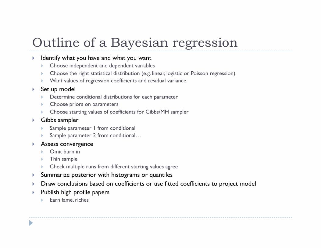
Outline of a Bayesian regression   Identify what you have and what you want

  Choose independent and dependent variables   Choose the right statistical distribution (e.g. linear, logistic or Poisson regression)   Want values of regression coefficients and residual variance

  Set up model   Determine conditional distributions for each parameter   Choose priors on parameters   Choose starting values of coefficients for Gibbs/MH sampler

  Gibbs sampler   Sample parameter 1 from conditional   Sample parameter 2 from conditional…

  Assess convergence   Omit burn in   Thin sample   Check multiple runs from different starting values agree

  Summarize posterior with histograms or quantiles   Draw conclusions based on coefficients or use fitted coefficients to project model   Publish high profile papers

  Earn fame, riches

Outline   Review   Continuation of exercises from last time

5

Exercise   Regression with Gibbs sampling from Clark 2007

  Models for Ecological Data   Statistical Computation for Environmental

Sciences with R

  Bonus Concepts/Jargon   Conjugate prior

Really Awesome

6

7

Conjugate Priors

€

The binomial pdf : Y = # success, n =# observations, Θ = prob of successBin(Y |θ)∝θ Y (1−θ )n−Y The beta pdf :Beta(θ |α,β)∝θα−1(1−θ)β −1

If the prior = Beta, likelihood = Binom, thenposterior =

p(θ |Y )∝θ Y (1−θ)n−Y [θα−1(1−θ )β −1] =θ Y +α−1(1−θ)n−Y +β −1

= Beta(θ |Y +α,n −Y + β)

What values of alpha and beta return the binomial distribution?

α=Y+1 β=n-Y+1

Binomial x Beta

8

Conjugate priors

0.1 0.3 0.5 0.7 0.9x

0

1

2

3

4

5

0.0 0.2 0.4 0.6 0.8 1.0

x

01

23

prior

0.0 0.2 0.4 0.6 0.8 1.0

x

01

23

prior

0.0 0.2 0.4 0.6 0.8 1.0

x

02

46

810

prior

Prior:

Beta(5,5)

Post:

Beta(22,12)

Prior:

Beta(10,3)

Post:

Beta(27,10)

Prior:

Beta(3,10)

Post:

Beta(20,17)

Prior:

Beta(100,30)

Post:

Beta(117,37)

Prior= grey, Post = red The mean of Beta (a,b) is a/(a+b)

Conjugate priors

From: http://www.johndcook.com/conjugate_prior_diagram.html#geometric 9

Arrow points from the distribution to its conjugate prior

A Bayesian regression model For the normal linear model, we have: yi ~ N(µi, σ2) for i ∈ 1,…,n

where µi is just an indicator for the expression: µi = B0 + B1X1i … + BkXki

The object of statistical inference is the posterior distribution of the parameters B0,…,Bk and σ2.

By Bayes Rule, we know that this is simply: p(B0,…,Bk, σ2 | Y, X) ∝ p(B0,…,Bk, σ2) × ∏i p(yi | µi, σ2) posterior prior likelihood

11

Bayesian regression with standard non-informative priors

  Posterior: p(B0,…,Bk, σ2 | Y, X) ∝ p(B0,…,Bk, σ2) × ∏i p(yi | µi, σ2)

  To make inferences about the regression coefficients, we need to choose a prior distribution for B, σ2.

  A conjugate prior for the Betas is a multivariate normal distribution – we choose large varaince to make it uninformative

  A conjugate prior for the variance is an inverse gamma distribution, also chosen to be uninformative.

Useful code for regression Exercise #This code is in the text, I’m just saving you some typing because its not critical to understand the mathematical details right now.

#b.update and v.update combine the likelihood and priors for the regression coeeficients and residual variance, respectively, and sample from the conditionals

b.update=function(y,sinv){

#y is the data vector

#sinv is the inverse of the variance

if(length(sinv)==1){ # if single variance parameter

sx=crossprod(x)*sinv

sy=crossprod(x,y)*sinv

}

if(length(sinv)>1){ # if covariance matrix

sx=t(x) %*% sinv %*% x

sy=t(x) %*% sinv %*% y

}

#the density of the betas are distributed as N(betas | bigv*smallv, bigV)

bigv=solve(sx+vinvert)

smallv=sy+vinvert %*% bprior

b=t(rmvnorm(1,bigv%*%smallv,bigv))

return(b)

}

v.update=function(y,rinverse){

#if no inverse correlation matrix (rinverse) use 1

if( length(rinverse)==1){ sx=crossprod((y-x%*%b))}

if( length(rinverse)>1){ sx=t(y-x%*%b) %*% rinverse %*% (y-x%*%b)}

u1=s1+.5*n

u2=s2+.5*sx

return(1/rgamma(1,u1,u2))

}

12

Exercise   Generalized Linear Regression from Clark 2007   Bonus Concepts/Jargon

  Nonconjugate priors   Metropolis-Hastings sampling   Jump distribution   Acceptance rates

13

Nonconjugate priors and Metropolis-Hastings (MH) sampling

  Sometimes the prior that describes your previous knowledge doesn’t have a functional form that combines nicely with with the likelihood

  In this example of logistic regression, a normal prior is used with the binomial likelihood

  Nonconjugate priors can lead to complex probability surfaces that would take a long time to explore, so MH makes the process more efficient

14

15

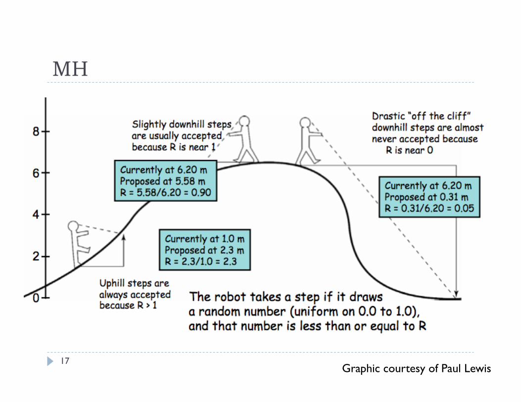
Metropolis-Hastings Sampling   In MH we reject some proposed steps that head toward

lower posterior density to save time by wandering mostly around high density regions

  Gibbs sampling is a special case of Metropolis -Hastings sampling but the value is always accepted

16

MH

Graphic courtesy of Paul Lewis

17

MH

Graphic courtesy of Paul Lewis

18

The Jump (Proposal) Distribution   One of most important and finicky parts of a successful

MH is the jump distribution   The jump distribution defines the proposed values and

you choose its parameters   Choose parameters so acceptance is 30-45%   A Metropolis step can be embedded within a Gibbs

sampling scheme to save time by performing the extra Metropolis calculations only when necessary

MH

19 Slide courtesy of Paul Lewis

MH

20 Slide courtesy of Paul Lewis

MH

21 Slide courtesy of Paul Lewis

GLM Exercise -Instructions and Useful code This is bonus code to analyze the model output

#acceptance rates

#note that either both parameters get accepted or neither do and it might be more efficient

# to accept each separately

n=2:ngibbs

sum(bgibbs[n,1]==bgibbs[n-1,1])/ngibbs

#to see the entire chain use the following

burn.and.thin=1:ngibbs

#to see the portion of the chain that you’d use for inference, with the burnin removed

#and thinning to avoid autocorrelation, use the following

# burnin sample thinning rate

#burn.and.thin=seq( .5*ngibbs , ngibbs , by=10)

beta.post=bgibbs[burn.and.thin,]

#plot diagnostics

par(mfcol=c(2,2))

#intercept

plot(beta.post[,1],type='l')

abline(h=b0,col='red')

plot(density(beta.post[,1],width=.4),type='l')

abline(v=quantile(beta.post[,1],c(.5,.025,.975)),col='blue')

#slope

plot(beta.post[,2],type='l')

abline(h=b1,col='red')

plot(density(beta.post[,2],width=.4),type='l')

abline(v=quantile(beta.post[,2],c(.5,.025,.975)),col='blue’)

#table summary outpar=matrix(NA,2,5) outpar[,1]=c(b0,b1) outpar[,2]=apply(beta.post,2,mean) outpar[,3]=apply(beta.post,2,sd) outpar[,4:5]=t(apply(beta.post,2,quantile,c(.025,.975))) colnames(outpar)=c('true','estimate','se','.025','.975') rownames(outpar)=c('b0','b1') signif(outpar,3)

Instructions: 1.  Start with 10,000 Gibbs samples here to

speed things up – this took about 20 s on my laptop

2.  Use this code after you’ve run the Gibbs sampler from the handout to look at the model output.

3.  See next slide for homework questions.

22

Exercise 2 - Questions   Notice anything funny about the model output? It doesn’t

appear to converge. Tinker around with model input to try to get the model to settle down. You want to see that (1) the posterior densities are relatively smooth, (2) that there are no long term trends in the trace plots, (3) acceptance rates are .3 - .45, (4) that the mean posterior parameter estimates are pretty close to the true parameter values (since we used simulated data). Once you think you’re in the right ballpark, run the model for 40,000 steps to check. You can adjust   Starting values   Jump distribution   Priors   Simulated data   Number of samples (don’t go crazy with this, it shouldn’t take more

than 20,000 to see some improvement) Continue to next slide….

23

Homework   Provide a 1-2 paragraph explanation of

  Why the model isn’t converging   Some of your attempted changes and why they might not have

worked   How you tried to solve those issues (you don’t have to make it

converge perfectly but you should be able to improve it)   Any relevant supporting model output

  Combine you answers with those from the hierarchical normal model that we’ll see shortly

  Email me a word doc with your answers with the subject heading ‘homework 2’

24