Bayesian DeepLearning

Mohammad Emtiyaz KhanAIP (RIKEN), Tokyo

http://emtiyaz.github.io

emtiyaz.khan@riken.jp

June 06, 2018

©Mohammad Emtiyaz Khan 2018

1

What will you learn?

Why is Bayesian inference useful?

1. It allows for computation of uncertainty.

2. It can prevent overfitting in a principled way.

Why is it computationally challenging?

3. It usually requires solving hard integrals.

How does Variational Inference (VI) simplify thecomputational challenge?

4. Integration is converted to an optimization problem.

5. Optimization gives a lower bound to the integral.

How to perform variational inference?

6. By using stochastic gradient descent.

1

1 Why be Bayesian?

Why be Bayesian

What are the main reasons behindthe recent success of Machine-learning and deep-learning meth-ods, e.g., in fields such as computervision, speech recognition, andrecommendation systems?

Existing methods focus on fittingthe data well (e.g., using maximumlikelihood), but this may be prob-lematic.

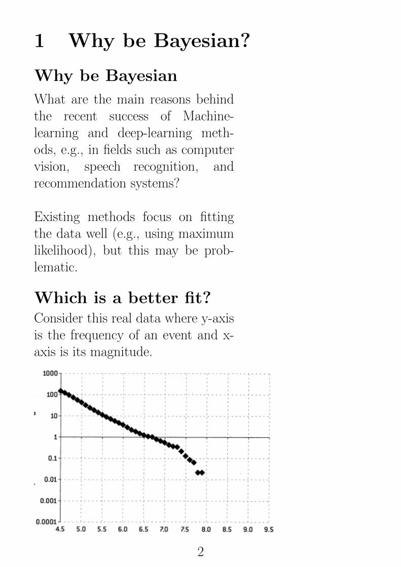
Which is a better fit?Consider this real data where y-axisis the frequency of an event and x-axis is its magnitude.

2

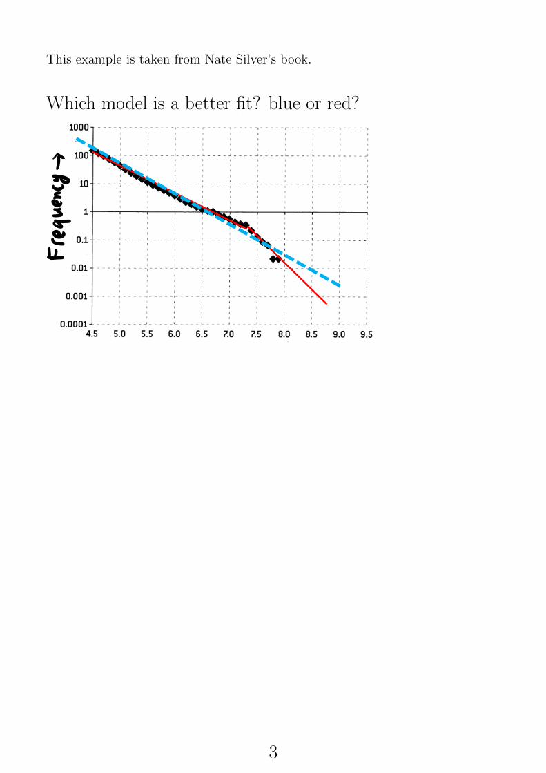
This example is taken from Nate Silver’s book.

Which model is a better fit? blue or red?

3

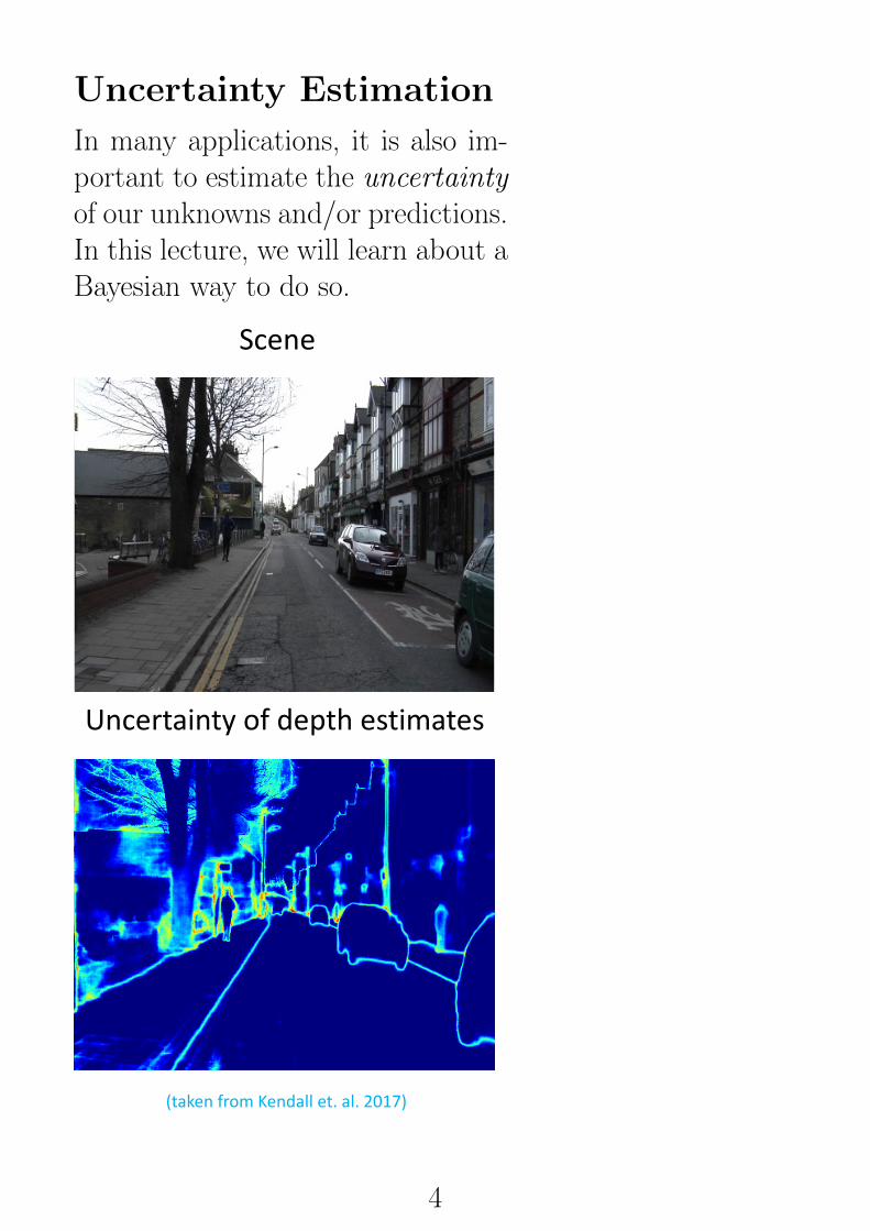
Uncertainty Estimation

In many applications, it is also im-portant to estimate the uncertaintyof our unknowns and/or predictions.In this lecture, we will learn about aBayesian way to do so.

(a) Input Image (b) Ground Truth (c) SemanticSegmentation

(d) AleatoricUncertainty

(e) EpistemicUncertainty

Figure 1: Illustrating the difference between aleatoric and epistemic uncertainty for semantic segmentationon the CamVid dataset [8]. Aleatoric uncertainty captures noise inherent in the observations. In (d) our modelexhibits increased aleatoric uncertainty on object boundaries and for objects far from the camera. Epistemicuncertainty accounts for our ignorance about which model generated our collected data. This is a notablydifferent measure of uncertainty and in (e) our model exhibits increased epistemic uncertainty for semanticallyand visually challenging pixels. The bottom row shows a failure case of the segmentation model when themodel fails to segment the footpath due to increased epistemic uncertainty, but not aleatoric uncertainty.

which captures our ignorance about which model generated our collected data. This uncertaintycan be explained away given enough data, and is often referred to as model uncertainty. Aleatoricuncertainty can further be categorized into homoscedastic uncertainty, uncertainty which stays con-stant for different inputs, and heteroscedastic uncertainty. Heteroscedastic uncertainty depends onthe inputs to the model, with some inputs potentially having more noisy outputs than others. Het-eroscedastic uncertainty is especially important for computer vision applications. For example, fordepth regression, highly textured input images with strong vanishing lines are expected to result inconfident predictions, whereas an input image of a featureless wall is expected to have very highuncertainty.

In this paper we make the observation that in many big data regimes (such as the ones commonto deep learning with image data), it is most effective to model aleatoric uncertainty, uncertaintywhich cannot be explained away. This is in comparison to epistemic uncertainty which is mostlyexplained away with the large amounts of data often available in machine vision. We further showthat modeling aleatoric uncertainty alone comes at a cost. Out-of-data examples, which can beidentified with epistemic uncertainty, cannot be identified with aleatoric uncertainty alone.

For this we present a unified Bayesian deep learning framework which allows us to learn map-pings from input data to aleatoric uncertainty and compose these together with epistemic uncer-tainty approximations. We derive our framework for both regression and classification applicationsand present results for per-pixel depth regression and semantic segmentation tasks (see Figure 1 andthe supplementary video for examples). We show how modeling aleatoric uncertainty in regressioncan be used to learn loss attenuation, and develop a complimentary approach for the classificationcase. This demonstrates the efficacy of our approach on difficult and large scale tasks.

The main contributions of this work are;

1. We capture an accurate understanding of aleatoric and epistemic uncertainties, in particularwith a novel approach for classification,

2. We improve model performance by 1 � 3% over non-Bayesian baselines by reducing theeffect of noisy data with the implied attenuation obtained from explicitly representingaleatoric uncertainty,

3. We study the trade-offs between modeling aleatoric or epistemic uncertainty by character-izing the properties of each uncertainty and comparing model performance and inferencetime.

2

Scene

(a) Input Image (b) Ground Truth (c) SemanticSegmentation

(d) AleatoricUncertainty

(e) EpistemicUncertainty

Figure 1: Illustrating the difference between aleatoric and epistemic uncertainty for semantic segmentationon the CamVid dataset [8]. Aleatoric uncertainty captures noise inherent in the observations. In (d) our modelexhibits increased aleatoric uncertainty on object boundaries and for objects far from the camera. Epistemicuncertainty accounts for our ignorance about which model generated our collected data. This is a notablydifferent measure of uncertainty and in (e) our model exhibits increased epistemic uncertainty for semanticallyand visually challenging pixels. The bottom row shows a failure case of the segmentation model when themodel fails to segment the footpath due to increased epistemic uncertainty, but not aleatoric uncertainty.

which captures our ignorance about which model generated our collected data. This uncertaintycan be explained away given enough data, and is often referred to as model uncertainty. Aleatoricuncertainty can further be categorized into homoscedastic uncertainty, uncertainty which stays con-stant for different inputs, and heteroscedastic uncertainty. Heteroscedastic uncertainty depends onthe inputs to the model, with some inputs potentially having more noisy outputs than others. Het-eroscedastic uncertainty is especially important for computer vision applications. For example, fordepth regression, highly textured input images with strong vanishing lines are expected to result inconfident predictions, whereas an input image of a featureless wall is expected to have very highuncertainty.

In this paper we make the observation that in many big data regimes (such as the ones commonto deep learning with image data), it is most effective to model aleatoric uncertainty, uncertaintywhich cannot be explained away. This is in comparison to epistemic uncertainty which is mostlyexplained away with the large amounts of data often available in machine vision. We further showthat modeling aleatoric uncertainty alone comes at a cost. Out-of-data examples, which can beidentified with epistemic uncertainty, cannot be identified with aleatoric uncertainty alone.

For this we present a unified Bayesian deep learning framework which allows us to learn map-pings from input data to aleatoric uncertainty and compose these together with epistemic uncer-tainty approximations. We derive our framework for both regression and classification applicationsand present results for per-pixel depth regression and semantic segmentation tasks (see Figure 1 andthe supplementary video for examples). We show how modeling aleatoric uncertainty in regressioncan be used to learn loss attenuation, and develop a complimentary approach for the classificationcase. This demonstrates the efficacy of our approach on difficult and large scale tasks.

The main contributions of this work are;

1. We capture an accurate understanding of aleatoric and epistemic uncertainties, in particularwith a novel approach for classification,

2. We improve model performance by 1 � 3% over non-Bayesian baselines by reducing theeffect of noisy data with the implied attenuation obtained from explicitly representingaleatoric uncertainty,

3. We study the trade-offs between modeling aleatoric or epistemic uncertainty by character-izing the properties of each uncertainty and comparing model performance and inferencetime.

2

(takenfromKendallet.al.2017)

Uncertaintyofdepthestimates

4

2 Bayesian Model for Regression

Regression

Regression is to relate input vari-ables to the output variable, to ei-ther predict outputs for new inputsand/or to understand the effect ofthe input on the output.

Dataset for regression

In regression, data consists of pairs(xn, yn), where xn is a vector of Dinputs and yn is the n’th output.Number of pairs N is the data-sizeand D is the dimensionality.

PredictionIn prediction, we wish to predictthe output for a new input vec-tor, i.e., find a regression functionthat approximates the output “wellenough” given inputs.

yn ≈ fθ(xn), for all n

where θ is the parameter of the re-gression model.

5

LikelihoodAssume yn to be independent sam-ples from an exponential family dis-tribution, whose mean parameter isequal to fθ(xn):

p(y|X) =

N∏n=1

p(yn|fθ(xn))

For example, when p is a Gaussian,the log-likelihood results in mean-square error.

Examples of fθ

Linear model: θ>xn

Generalized: f (θ>xn)

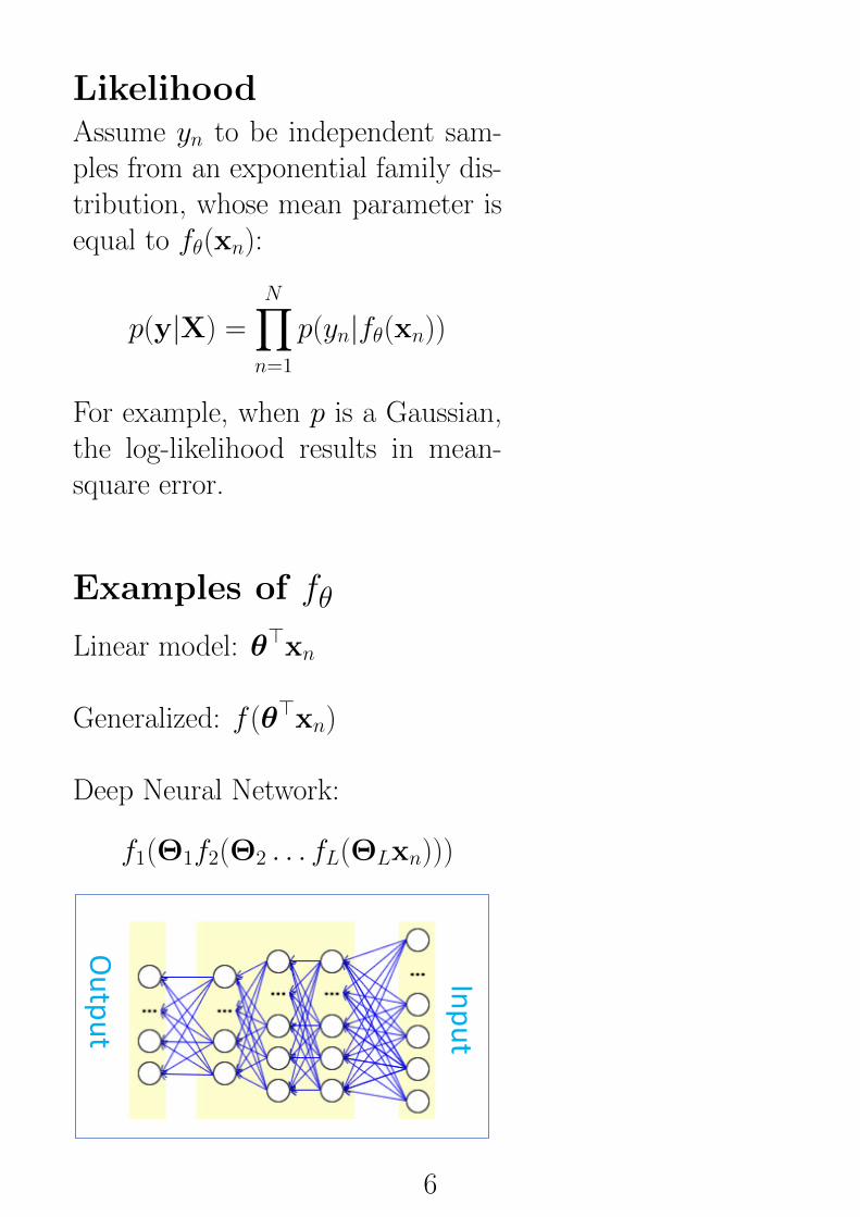
Deep Neural Network:

f1(Θ1f2(Θ2 . . . fL(ΘLxn)))

Input

Output

6

Maximum A Posteriori (MAP)

By using a regularizer log p(θ),we can estimate θ by maximiz-ing the following loss denoted byLMAP (θ) :=

N∑n=1

log p(yn|fθ(xn)) + log p(θ)

Example: an L2 regularizer. TheθMAP obtained by maximizingLMAP is known as the maximum-a-posteriori estimate.

Stochastic Gradient Descent (SGD)

When N is large, choose a randompair (xn, yn) in the training set andapproximate the gradient:

∂LMAP

∂θ≈ ∂

∂θ[N log p(yn|fθ(xn)) + log p(θ)]

Using the above stochastic gradient,take a step:

θt+1 = θt + ρt∂̂LMAP

∂θ

where t is the iteration, and ρt is alearning rate.

7

The Joint DistributionHow can we obtain a distributionover θ? We can make use of theBayes’ rule.

We can view p(θ) as a prior distri-bution to define the following jointdistribution:

log p(y,θ|X)

:=

N∑n=1

log p(yn|fθ(xn)) + log p(θ) + cnst

= log

[N∏n=1

p(yn|fθ(xn))

]p(θ)

For example: L2 loss corresponds toa Gaussian prior distribution.

8

The Posterior DistributionThe posterior distribution is definedusing the Bayes’ rule:

p(θ|y,X) =p(y,θ|X)

p(y|X)

=

[∏Nn=1 p(yn|fθ(xn))

]p(θ)∫ [∏N

n=1 p(yn|fθ(xn))]p(θ)dθ

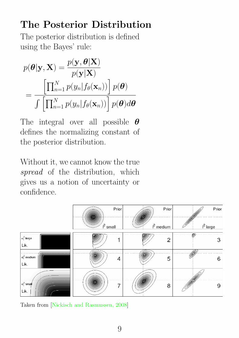
The integral over all possible θdefines the normalizing constant ofthe posterior distribution.

Without it, we cannot know the truespread of the distribution, whichgives us a notion of uncertainty orconfidence.

Taken from [Nickisch and Rasmussen, 2008]

9

Difficult Integral

The normalizing constant of the pos-terior distribution is difficult to com-pute in general:

p(y|X) =

∫ [ N∏n=1

p(yn|fθ(xn))

]p(θ)dθ

There are (at least) three reasonsbehind it:

1) Too many factors (large N)2) Too many dimensions (large D)3) Nonconjugacy (e.g., non Gaussianlikelihood with a Gaussian prior)

10

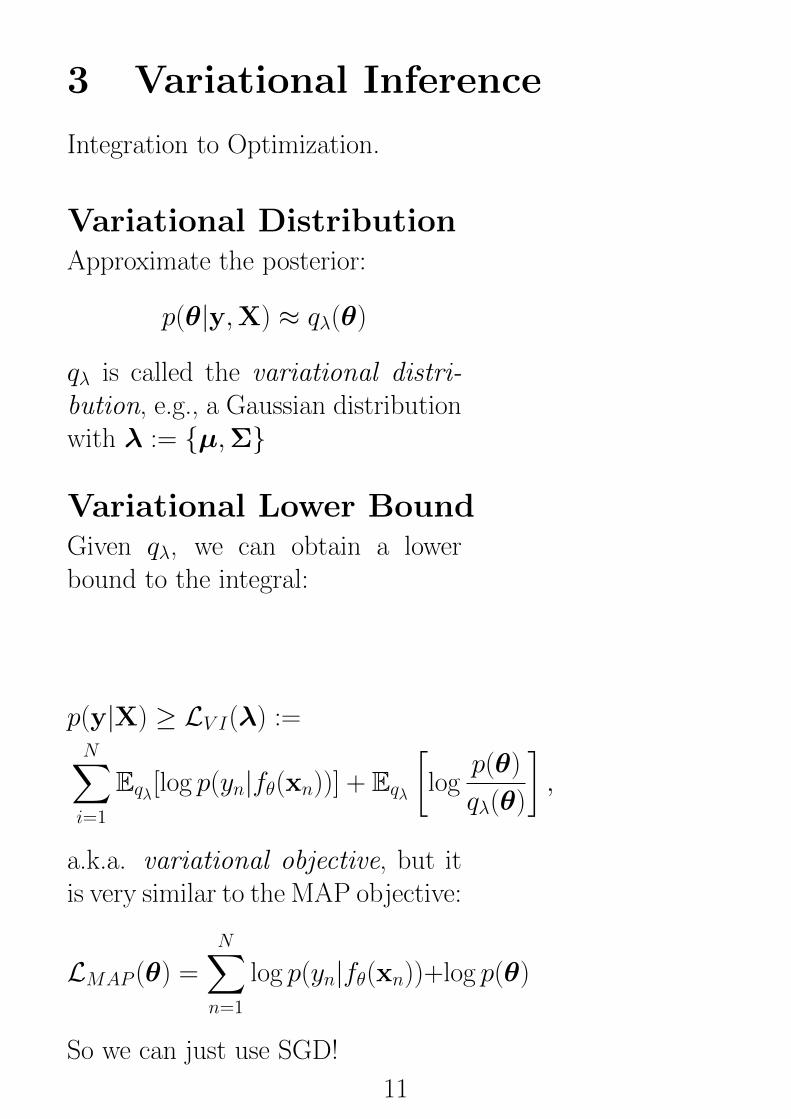
3 Variational Inference

Integration to Optimization.

Variational DistributionApproximate the posterior:

p(θ|y,X) ≈ qλ(θ)

qλ is called the variational distri-bution, e.g., a Gaussian distributionwith λ := {µ,Σ}

Variational Lower BoundGiven qλ, we can obtain a lowerbound to the integral:

p(y|X) ≥ LV I(λ) :=N∑i=1

Eqλ[log p(yn|fθ(xn))] + Eqλ

[log

p(θ)

qλ(θ)

],

a.k.a. variational objective, but itis very similar to the MAP objective:

LMAP (θ) =

N∑n=1

log p(yn|fθ(xn))+log p(θ)

So we can just use SGD!

11

Stochastic Gradients IHow do we compute a stochasticgradient of LV I? The reparameter-ization trick is one method to doso [Kingma and Welling, 2013]. Letqλ := N (z|µ, diag(σ2)), then

θ(λ) = µ + σ ◦ ε, ε ∼ N (ε|0, I)

is a sample from qλ. We have writtenθ as a function of λ := {µ,σ}.

Here is a stochastic gradient withone Monte-Carlo sample θ(λ):

∂LV I(λ)

∂λ≈ ∂θ

∂λ

∂LMAP (θ)

∂θ

− ∂θ

∂λ

∂log qλ(θ)

∂θ− ∂log qλ(θ)

∂λ

This can be done whenever qλ isreparameterizable.

12

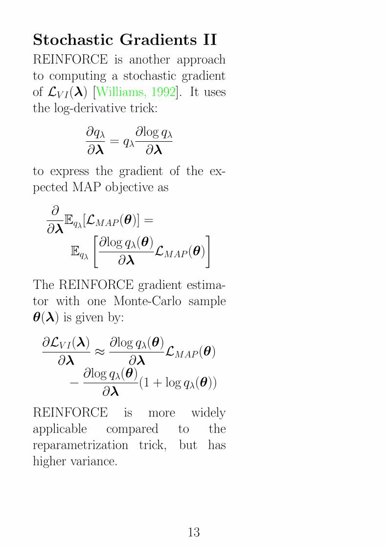
Stochastic Gradients IIREINFORCE is another approachto computing a stochastic gradientof LV I(λ) [Williams, 1992]. It usesthe log-derivative trick:

∂qλ∂λ

= qλ∂log qλ∂λ

to express the gradient of the ex-pected MAP objective as

∂

∂λEqλ[LMAP (θ)] =

Eqλ

[∂log qλ(θ)

∂λLMAP (θ)

]The REINFORCE gradient estima-tor with one Monte-Carlo sampleθ(λ) is given by:

∂LV I(λ)

∂λ≈ ∂log qλ(θ)

∂λLMAP (θ)

− ∂log qλ(θ)

∂λ(1 + log qλ(θ))

REINFORCE is more widelyapplicable compared to thereparametrization trick, but hashigher variance.

13

Homework

1. Derive the expression for REINFORCE.

2. VI for Linear regression

(a) Derive the variational lower bound for a linear-regression

problem. Assume a Gaussian prior on θ.

(b) What kind of posterior approximation is appropriate in this

case?

(c) When will the lower bound be tight?

(d) What is the memory and computational complexity of SGD?

14

References

[Kingma and Welling, 2013] Kingma, D. P. and Welling, M.

(2013). Auto-encoding variational Bayes. arXiv preprint

arXiv:1312.6114.

[Nickisch and Rasmussen, 2008] Nickisch, H. and Ras-

mussen, C. (2008). Approximations for binary Gaussian

process classification. Journal of Machine Learning

Research, 9(10).

[Williams, 1992] Williams, R. J. (1992). Simple statistical

gradient-following algorithms for connectionist reinforce-

ment learning. Machine learning, 8(3-4):229–256.

15

Extra space

16

Extra space

17