a uniÞed approach to building and controlling spiking...

LETTER Communicated by Daniel Durstewitz

A Unified Approach to Building and Controlling SpikingAttractor Networks

Chris EliasmithceliasmithuwaterloocaDepartment of Philosophy and Department of Systems Design EngineeringUniversity of Waterloo Waterloo Ontario Canada

Extending work in Eliasmith and Anderson (2003) we employ a generalframework to construct biologically plausible simulations of the threeclasses of attractor networks relevant for biological systems static (pointline ring and plane) attractors cyclic attractors and chaotic attractors Wediscuss these attractors in the context of the neural systems that they havebeen posited to help explain eye control working memory and head di-rection locomotion (specifically swimming) and olfaction respectivelyWe then demonstrate how to introduce control into these models Theaddition of control shows how attractor networks can be used as subsys-tems in larger neural systems demonstrates how a much larger class ofnetworks can be related to attractor networks and makes it clear howattractor networks can be exploited for various information processingtasks in neurobiological systems

1 Introduction

Persistent activity has been thought to be important for neural computa-tion at least since Hebb (1949) who suggested that it may underlie short-term memory Amit (1989) following work on attractors in artificial neuralnetworks (eg that of Hopfield 1982) suggested that persistent neural ac-tivity in biological networks is a result of dynamical attractors in the statespace of recurrent networks Since then attractor networks have become amainstay of computational neuroscience and have been used in a widevariety of models (see eg Zhang 1996 Seung Lee Reis amp Tank 2000Touretzky amp Redish 1996 Laing amp Chow 2001 Hansel amp Sompolinsky 1998Eliasmith Westover amp Anderson 2002) Despite a general agreementamong theoretical neuroscientists that attractor networks form a large andbiologically relevant class of networks there is no general method for con-structing and controlling the behavior of such networks In this letter wepresent such a method and explore several examples of its application sig-nificantly extending work described in Eliasmith and Anderson (2003) Weargue that this framework can both unify the current use of attractor net-works and show how to extend the range of applicability of attractor models

Neural Computation 17 1276ndash1314 (2005) copy 2005 Massachusetts Institute of Technology

Controlling Spiking Attractor Networks 1277

Most important perhaps we describe in detail how complex control can beintegrated with standard attractor models This allows us to begin to an-swer the kinds of pressing questions now being posed by neuroscientistsincluding for example how to account for the dynamics of working mem-ory (see eg Brody Romo amp Kepecs 2003 Fuster 2001 Rainer amp Miller2002)

We briefly summarize the general framework and then demonstrate itsapplication to the construction of spiking networks that exhibit line planering cyclic and chaotic attractors Subsequently we describe how to inte-grate control signals into each of these models significantly increasing thepower and range of application of these networks

2 Framework

This section briefly summarizes the methods described in Eliasmith andAnderson (2003) which we will refer to as the neural engineering frame-work (NEF) Subsequent sections discuss the application of these methodsto the construction and control of attractor networks The following threeprinciples describe the approach

1 Neural representations are defined by the combination of nonlinearencoding (exemplified by neuron tuning curves and neural spiking)and weighted linear decoding (over populations of neurons and overtime)

2 Transformations of neural representations are functions of the vari-ables represented by neural populations Transformations are deter-mined using an alternately weighted linear decoding

3 Neural dynamics are characterized by considering neural representa-tions as control-theoretic state variables Thus the dynamics of neu-robiological systems can be analyzed using control theory

In addition to these main principles the following addendum is taken to beimportant for analyzing neural systems

Neural systems are subject to significant amounts of noise Thereforeany analysis of such systems must account for the effects of noise

Each of the next three sections describes one of the principles in the con-text of the addendum in more detail (For detailed justifications of theseprinciples see Eliasmith amp Anderson 2003) They are presented here tomake clear both the terminology and assumptions in the subsequent net-work derivations The successes of the subsequent models help to justifythe adoption of these principles

1278 C Eliasmith

21 Representation Consider a population of neurons whose activitiesai (x) encode some vector x These activities can be written as

ai (x) = Gi [J i (x)] (21)

where Gi is the nonlinear function describing the neuronrsquos response func-tion and J i (x) is the current entering the soma The somatic current is givenby

J i (x) = αi 〈x middot φi 〉 + J biasi (22)

where αi is a gain and conversion factor x is the vector variable to be en-coded φi determines the preferred stimulus of the neuron and J bias

i is abias current that accounts for background activity This equation providesa standard description of the effects of a current arriving at the soma ofneuron i as a result of presenting a stimulus x

The nonlinearity Gi that describes the neuronrsquos activity as a result ofthis current can be left undefined for the moment In general it should bedetermined experimentally and thus based on the intrinsic physiologicalproperties of the neuron(s) being modeled The result of applying Gi to thesoma current J i (x) over the range of stimuli gives the neuronrsquos tuning curveai (x) So ai (x) defines the encoding of the stimulus into neural activity

Given this encoding the original stimulus vector can be estimated bydecoding those activities for example

x =sum

i

ai (x)φi (23)

These decoding vectors φi can be found by a least-squares method (see theappendix Salinas amp Abbott 1994 Eliasmith amp Anderson 2003) Togetherthe nonlinear encoding in equation 21 and the linear decoding in equation23 define a neural population code for the representation of x

To incorporate a temporal code into this population code we can draw onwork that has shown that most of the information in neural spike trains canbe extracted by linear decoding (Rieke Warland de Ruyter van Steveninckamp Bialek 1997) Let us first consider the temporal code in isolation by takingthe neural activities ai (t) to be decoded spike trains that is

ai (t) =sum

n

hi (t) lowast δi (t minus tn) =sum

n

hi (t minus tn) (24)

where δi (middot) are the spikes at times tn for neuron i and hi (t) are the lineardecoding filters which for reasons of biological plausibility we can take tobe the (normalized) postsynaptic currents (PSCs) in the subsequent neuronElsewhere it has been shown that the information loss under this assumptionis minimal and can be alleviated by increasing population size (Eliasmith


amp Anderson 2003) As before the encoding on which this linear decodingoperates is defined as in equation 21 where Gi is now taken to be a spikingnonlinearity

We can now combine this temporal code with the previously definedpopulation code to give a general population temporal code for vectors

δ(t minus tin) = Gi[αi 〈x middot φi 〉 + J bias

i

]Encoding

x = sumin hi (t minus tn)φi Decoding

22 Transformation For such representations to be useful they mustbe used to define transformations (ie functions of the vector variables)Fortunately we can again find (least-squares optimal) decoders φ

f (x)i to

perform a transformation f (x) So instead of finding the optimal decodersφi to extract the originally encoded variable x from the encoding we canreweight the decoding to give some function f (x) other than identity (see theappendix) To distinguish the representational decoders φi from φ

f (x)i we

refer to the latter as transformational decoders Given this characterizationit is a simple matter to rewrite the encoding and decoding equations forestimating some function of the vector variable


i

]Encoding

f (x) = sumin hi (t minus tn)φ f (x)

i Decoding

Notably both linear and nonlinear functions of the encoded variable canbe computed in this manner (see Eliasmith amp Anderson 2003 for furtherdiscussion)

23 Dynamics Dynamics of neural systems can be described using theprevious characterizations of representation and transformation by employ-ing modern control theory Specifically we can allow the higher-level vectorvariables represented by a neural population to be control-theoretic statevariables

Let us first consider linear time-invariant (LTI) systems Recall that thestate equation in modern control theory describing LTI dynamics is

x(t) = Ax(t) + Bu(t) (25)

The input matrix B and the dynamics matrix A completely describe thedynamics of the LTI system given the state variables x(t) and the input u(t)Taking the Laplace transform of equation 25 gives

x(s) = h(s) [Ax(s) + Bu(s)]

where h(s) = 1s Any LTI control system can be written in this form

1280 C Eliasmith

In the case of neural systems the transfer function h(s) is not 1s but is

determined by the intrinsic properties of the component cells Because it isreasonable to assume that the dynamics of the synaptic PSC dominate thedynamics of the cellular response as a whole (Eliasmith amp Anderson 2003)it is reasonable to characterize the dynamics of neural populations basedon their synaptic dynamics that is using hi (t) from equation 24

A simple model of a synaptic PSC is given by

hprime(t) = 1τ

eminustτ (26)

where τ is the synaptic time constant The Laplace transform of this filter is

hprime(s) = 11 + sτ

Given the change in filters from h(s) to hprime(s) we now need to determinehow to change A and B in order to preserve the dynamics defined in theoriginal system (ie the one using h(s)) In other words letting the neu-ral dynamics be defined by Aprime and Bprime we need to determine the relationbetween matrices A and Aprime and matrices B and Bprime given the differences be-tween h(s) and hprime(s) To do so we can solve for x(s) in both cases and equatethe resulting expressions for x(s) This gives

Aprime = τA + I (27)

Bprime = τB (28)

This procedure assumes nothing about A or B so we can construct a neu-robiologically realistic implementation of any dynamical system definedusing the techniques of modern control theory applied to LTI systems (con-strained by the neuronsrsquo intrinsic dynamics) Note also that this derivationis independent of the spiking nonlinearity since that process is both veryrapid and dedicated to encoding the resultant somatic voltage (not filteringit in any significant way) Importantly the same approach can be used tocharacterize the broader class of time-varying and nonlinear control systems(examples are provided below)

24 Synthesis Combining the preceding characterizations of represen-tation transformation and dynamics results in the generic neural subsys-tem shown in Figure 1 With this formulation the synaptic weights neededto implement some specified control system can be directly computed Notethat the formulation also provides for simulating the same model at variouslevels of description (eg at the level of neural populations or individualneurons using either rate neurons or spiking neurons and so on) This isuseful for fine-tuning a model before introducing the extra computationaloverhead involved with modeling complex spiking neurons


Mαβ

Mαβ

1jFβ

jFβ

iα Gi[]

Jiα(t)

synaptic weights

soma

higher-level description

neural description

1

sim

PSCs

dendrites

Fαβ[xβ(t)]

Fαβ[xβ(t)]1+sτij

Σδα(t-tin)n

Σδβ

Σδβ

(t-tjn)n

(t-tjn)n

αβ

1+sτijαβ

φ

φ

φ

Figure 1 A generic neural population systems diagram This figure is a combi-nation of a higher-level (control-theoretic) and a neural-level system description(denoted by dotted lines) The solid boxes highlight the dendritic elements Theright-most solid box decomposes the synaptic weights into the relevant matri-ces See the text for further discussion (Adapted from Eliasmith amp Anderson2003)

In Figure 1 the solid lines highlight the dendritic components whichhave been separated into postsynaptic filtering by the PSCs (ie temporaldecoding) and the synaptic weights (population decoding and encoding)The weights themselves are determined by three matrices (1) the decodingmatrix whose elements are the decoders φ

Fβ

i for some (nonlinear) functionF of the signal xβ (t) that comes from a preceding population β (2) the en-coding matrix whose elements are the encoders φα

i for this population and(3) the generalized transformation matrix Mαβ which defines the transfor-mations necessary for implementing the desired control system

Essentially this diagram summarizes the three principles and their in-terrelations The generality of the diagram hints at the generality of the un-derlying framework In the remainder of the article however I focus onlyon its application to the construction and control of attractor networks

3 Building Attractor Networks

The most obvious feature of attractor networks is their tendency towarddynamic stability That is given a momentary input they will settle on aposition or a recurring sequence of positions in state space This kind ofstability can be usefully exploited by biological systems in a number ofways For instance it can help the system react to environmental changes

1282 C Eliasmith

on multiple timescales That is stability permits systems to act on longertimescales than they might otherwise be able to which is essential fornumerous behaviors including prediction navigation and social interac-tion In addition stability can be used as an indicator of task completionsuch as in the case of stimulus categorization (Hopfield 1982) As wellstability can make the system more robust (ie more resistant to undesir-able perturbations) Because these networks are constructed so as to haveonly a certain set of stable states random perturbations to nearby statescan quickly dissipate to a stable state As a result attractor networks havebeen shown to be effective for noise reduction (Pouget Zhang Deneve ampLatham 1998) Similarly attractors over a series of states (eg cyclic attrac-tors) can be used to robustly support repetitive behaviors such as walkingswimming flying or chewing

Given these kinds of useful computational properties and their naturalanalogs in biological behavior it is unsurprising that attractor networkshave become a staple of computational neuroscience More than this asthe complexity of computational models continues to increase attractornetworks are likely to form important subnetworks in larger models Thisis because the ability of attractor networks to for example categorize filternoise and integrate signals makes them good candidates for being some ofthe basic building blocks of complex signal processing systems As a resultthe networks described here should prove useful for a wide class of morecomplex models

To maintain consistency all of the results of subsequent models weregenerated using networks of leaky integrate-and-fire neurons with abso-lute refractory periods of 1 ms membrane time constants of 10 ms andsynaptic time constants of 5 ms Intercepts and maximum firing rates werechosen from even distributions The intercept intervals are normalized over[minus1 1] unless otherwise specified (For a detailed discussion of the effectsof changing these parameters see Eliasmith amp Anderson 2003)

For each example presented below the presentation focuses specificallyon the construction of the relevant model As a result there is minimaldiscussion of the justification for mapping particular kinds of attractors ontovarious neural systems and behaviors although references are provided

31 Line Attractor The line attractor or neural integrator has recentlybeen implicated in decision making (Shadlen amp Newsome 2001 Wang2002) but is most extensively explored in the context of oculomotor con-trol (Fukushima Kaneko amp Fuchs 1992 Seung 1996 Askay GamkrelidzeSeung Baker amp Tank 2001) It is interesting to note that the terms line attrac-tor and neural integrator actually describe different aspects of the network Inparticular the network is called an integrator because the low-dimensionalvariable (eg horizontal eye position) x(t) describing the networkrsquos outputreflects the integration of the input signal (eg eye movement velocity) u(t)to the system In contrast the network is called a line attractor because in


u(t)

x(t)

A

B

bk(t) aj(t)

Figure 2 Line attractor network architecture The underline denotes variablesthat are part of the neuron-level description The remaining variables are partof the higher-level description

the high-dimensional activity space of the network (where the dimensionis equal to the number of neurons in the network) the organization of thesystem collapses network activity to lie on a one-dimensional subspace (iea line) As a result only input that moves the network along this line changesthe networkrsquos output

In a sense then these two terms reflect a difference between what canbe called higher-level and neuron-level descriptions of the system (seeFigure 2) As modelers of the system we need a method that allows usto integrate these two descriptions Adopting the principles outlined ear-lier does precisely this Notably the resulting derivation is simple and issimilar to that presented in Eliasmith and Anderson (2003) However all ofthe steps needed to generate the far more complex circuits discussed laterare described here so it is useful as an introduction (and referred to for someof the subsequent derivations)

We can begin by describing the higher-level behavior as integrationwhich has the state equation

x = Ax(t) + Bu(t) (31)

x(s) = 1s

[Ax(s) + Bu(s)] (32)

where A = 0 and B = 1 Given principle 3 we can determine Aprime and B primewhich are needed to implement this behavior in a system with neural dy-namics defined by hprime(t) (see equation 26) The result is

B prime = τ

Aprime = 1

1284 C Eliasmith

-1 -08 -06 -04 -02 0 02 04 06 08 10

50

100

150

200

250

x

Firi

ng R

ate

(Hz)

Figure 3 Sample tuning curves for a population of neurons used to implementthe line attractor These are the equivalent steady-state tuning curves of thespiking neurons used in this example They are found by solving the differentialequations for the leaky integrate-and-fire neuron assuming a constant inputcurrent and are described by a j (x) = 1

τrefj minusτRC

j ln(

1minus Jthresholda j x+J bias

)

where τ is the time constant of the PSC of neurons in the population repre-senting x(t)

To use this description in a neural model we must define the representa-tion of the state variable of the system x(t) Given principle 1 let us definethis representation using the following encoding and decoding

a j (t) = G j[α j 〈x(t)φ j 〉 + J bias

j

](33)

and

x(t) =sum

j

a j (t)φxj (34)

Note that the encoding weight φ j plays the same role as the encoding vectorin equation 22 but is simply plusmn1 (for on and off neurons) in the scalar caseFigure 3 shows a population of neurons with this kind of encoding Let usalso assume an analogous representation for u(t)

Working in the time domain we can take our description of the dynamics

x(t) = hprime(t) lowast [Aprimex(t) + B primeu(t)

]


and substitute it into equation 33 to give

a j (t) = G j[α j 〈φ j hprime(t) lowast [Aprimex(t) + B primeu(t)]〉 + J bias

j

] (35)

Substituting our decoding equation 34 into 35 for both populations gives

a j (t) = G j

[α j

langhprime(t) lowast φ j

[Aprime sum

i

ai (t)φxi + B prime sum

k

bk(t)φuk

]rang+ J bias

j

]

(36)

= G j

[hprime(t) lowast

[sumi

ω j i ai (t) +sum

k

ω jkbk(t)

]+ J bias

j

] (37)

where ω j i = α j Aprimeφxi φ j andω jk = α j B primeφu

k φ j are the recurrent and input con-nection weights respectively Note that i is used to index population activityat the previous time step1 and Gi is a spiking nonlinearity It is importantto keep in mind that the temporal filtering is done only once despite thisnotation That is hprime(t) is the same filter as that defining the decoding of bothx(t) and u(t) More precisely this equation should be written as

sumn

δ j (t minus tn) = G j

[sumin

ω j i hprimei (t) lowast δi (t minus tn) + (38)

sumkn

ω jkhprimek(t) lowast δk(t minus tn) + J bias

j

] (39)

The dynamics of this system when hprimei (t) = hprime

k(t) are as written inequation 35 which is the case of most interest as it best approximates a trueintegrator Nevertheless they do not have to be equal and model a broaderclass of dynamics when this is included in the higher-level analysis

For completeness we can write the subthreshold dynamical equationsfor an individual LIF neuron voltage Vj (t) in this population as follows

dVj

dt= minus 1

τRCj

(Vj minus Rj

[sumin


sumkn


j

]) (311)

1 In fact there are no discrete time steps since this is a continuous system Howeverthe PSC effectively acts as a time step as it determines the length of time that previousinformation is available

1286 C Eliasmith

0 01 02 03 04 05 06 07 08 09 1

0

1

0

1

u(t)

A)

B)

Time (s)

0

10

20

30

40

50

60

70

Neu

ron

Time (s)

C)

x(t)

-1

0 01 02 03 04 05 06 07 08 09 10 01 02 03 04 05 06 07 08 09 1

Figure 4 (A) The decoded input u(t) (B) the decoded integration x(t) of a spik-ing line attractor with 200 neurons under 10 noise and (C) spike rasters of athird of the neurons in the population

where τRCj = Rj C j Rj is the membrane resistance and C j the membrane

capacitance As usual the spikes are determined by choosing a thresholdvoltage for the LIF neuron (Vth) and placing a spike when Vj gt Vth In ourmodels we also include a refractory time constant τ

refj which captures the

absolute refractory period observed in real neurons Figure 4 shows a briefsample run for this network

To gain insight into the networkrsquos function as both an attractor and anintegrator it is important to derive measures of the networkrsquos behavior Thishas already been done to some extent for line attractors so I will not discusssuch measures here (Seung et al 2000 Eliasmith amp Anderson 2003) Whatthese analyses make clear however is how higher-level properties such asthe effective time constant of the network are related to neuron-level prop-erties such as membrane and synaptic time constants Because the previousderivation is part of a general method for building more complex attractornetworks (as I discuss next) it becomes evident how these same analysescan apply in the more complex cases This is a significant benefit of generat-ing models with a set of unified principles More important from a practicalstandpoint constructing this network by employing control theory makesit evident how to control some of the high-level properties such as the effec-tive network time constant (see section 4) It is this kind of control that beginsto make clear how important such simple networks are for understandingneural signal processing

32 Plane Attractor Perhaps the most obvious generalization of a lineattractor is to a plane attractor that is from a one-dimensional to a multidi-mensional attractor In this section I perform this generalization Howeverto demonstrate the representational generality of the NEF I consider plane


attractors in the context of function representation (rather than vector repre-sentation) This has the further benefit of demonstrating how the ubiquitousbump attractor networks relate to the methods described here

Networks that have sustained gaussian-like bumps of activity have beenposited in various neural systems including frontal working memory areas(Laing amp Chow 2001 Brody et al 2003) the head direction system (Zhang1996 Redish 1999) visual feature selection areas (Hansel amp Sompolinsky1998) arm control systems (Snyder Batista amp Andersen 1997) and the pathintegration system (Conklin amp Eliasmith 2005) The prevalence of this kindof attractor suggests that it is important to account for such networks in ageneral framework However it is not immediately obvious how the stablerepresentation of functions relates to either vector or scalar representationas I have so far described it

Theoretically continuous function representation demands an infinitenumber of degrees of freedom Neural systems of course are finite As aresult it is natural to assume that understanding function representationin neural systems can be done using a finite basis for the function spaceaccessible by that system Given a finite basis the finite set of coefficients ofsuch a basis determines the function being represented by the system at anytime As a result function representation can be treated as the representationof a vector of coefficients over some basis that is

x(ν A) =Msum

m=1

xmm(ν) (312)

where ν is the dimension the function is defined over (eg spatial position)x is the vector of M coefficients xm and m are the set of M orthonormalbasis functions needed to define the function space Notably this basis doesnot need to be accessible in any way by the neural system itself it is merely away for us to conveniently write the function space that can be representedby the system

The neural representation depends on an overcomplete representationof this same space where the overcomplete basis is defined by the tuningcurves of the relevant neurons More specifically we can define the encodingof a function space analogous to that for a vector space by writing

ai (x(ν x)) = ai (x) = Gi[αi 〈x(ν x)φi (ν)〉ν + J bias

i

] (313)

Here the encoded function x(ν x) (eg a gaussian-like bump) and the en-coding function φi (ν) which is inferred from the tuning curve determinethe activity of the neuron Because of the integration over ν in this encodingit is only changes in the coefficients x that affect neural firing again making

1288 C Eliasmith

it clear that we can treat neural activity as encoding a vector of coefficientsThe decoding for function representation is as expected

x(ν x) =sum

i

ai (x)φi (ν) (314)

where the decoders φi (ν) can be determined like the vector decoders dis-cussed earlier

Having defined the function representation in this way we are in a po-sition to explicitly relate it to an equivalent vector representation This isimportant because it allows us to use the control-theoretic techniques dis-cussed in section 23 to define the dynamics of the representation Let usbegin by writing the decoders φi (ν) using the orthonormal basis that de-fines the function space x(ν x)

φi (ν) =Msumm

qimm(ν)

where qim are elements of the matrix of coefficients defining each of the iencoding functions with respect to the basis m(ν) This ensures that therepresentation of a given function will not lie outside the original func-tion space Similarly the encoding functions φi (ν) should encode functionsx(ν x) only in such a way that they can be decoded by these decoders sowe may assume

φi (ν) =Msumm

qimm(ν) (315)

Together these definitions determine the equivalent of the function rep-resentation in a vector space In particular the encoding is given by

ai (x) = Gi

[αi

langsumnm

xmm(ν)qinn(ν)

rangν

+ J biasi

]

= Gi

[αi

(sumnm

xmqinδnm

)+ J bias

i

]

= Gi

[αi

(summ

xmqim

)+ J bias

i

]

= Gi[αi 〈xqi 〉m + J bias

i

]


-1 -08 -06 -04 -02 0 02 04 06 08 1

-01

0

01

ν

Φ(ν

)

Φ1Φ2Φ3Φ4Φ5

-3 -2 -1 0 1 2 3-01

0

01

ν

Φ1Φ2Φ3ΦΦ

4

5

A) B)

Φ(ν

)

Figure 5 The orthonormal bases for the representational spaces for (A) the ringattractor in the head direction system and (B) LIP working memory Note thatthe former is cyclic and the latter is not

and the decoding is given by

x =sum

i

ai (x)qi

Essentially these equations simply convert the encoding and decoding func-tions into their equivalent encoding and decoding vectors in the functionspace whose dimensions are determined by m Our description of a neuralsystem in this space will have all the same properties as it did in the originalfunction space The advantage as already mentioned is that control theoryis more easily applied to finite vector spaces When we introduce control insection 4 we demonstrate this advantage in more detail

To see the utility of this formulation let us consider two different neuralsystems in parallel working memory in lateral intraparietal (LIP) cortexand the ring attractor in the head direction system2 These can be consideredin parallel because the dominant dynamics in both systems are the sameThat is just like the integrator LIP working memory and the ring attractormaintain a constant value with no input x = 0

The difference between these systems is that LIP working memory issometimes taken to have a bounded domain of representation (eg betweenplusmn60 degrees from midline) whereas the ring attractor has a cyclic domainof representation Given equation 312 this difference will show up as adifference in the orthonormal basis (ν) that spans the representationalspace Figure 5 shows this difference

2 The first of these is considered in Eliasmith amp Anderson (2003) although without theintegration of the data as described here

1290 C Eliasmith

A) B)

Figure 6 Samples of the (A) encoding functions and (B) resultant tuning curvesfor LIP neurons based on the data provided in Platt and Glimcher (1998)

In fact these orthonormal basis functions can be inferred from the neuraldata To do so we first need to construct the neural encoding functions φi (ν)by looking at the experimentally determined tuning curves of the neuronsThat is we can generate a population of neurons with tuning curves thathave the same distribution of widths and heights as observed in the systemwe are modeling and then use the encoding functions necessary for gen-erating that population as an overcomplete basis for the representationalspace We can then determine using singular value decomposition theorthonormal basis that spans that same space and use it as our orthonor-mal basis (ν) For example using data from Platt and Glimcher (1998)we have applied this method to get the tuning curves shown in Figure 6Athe encoders shown in Figure 6B and thus arrive at the orthonormal basisshown in Figure 5B for LIP representation

Given an orthonormal basis we now need to determine which set ofcoefficients x on that basis is relevant for the neural system of interest Thestandard representations in both LIP working memory and the ring attractorare generally characterized as gaussian-like bumps at any position How-ever in LIP there is evidence that this bump can be further parameterizedby nonpositional dimensions (Sereno amp Maunsell 1998) This kind of para-metric working memory has also been found in frontal systems (RomoBrody Hernandez amp Lemus 1999) So the representation in LIP will begaussian-like bumps but of varying heights

Ideally we need to specify some probability density ρ(x) on the coeffi-cients that appropriately picks out just the gaussian-like functions centeredat every value of ν (and those of various heights for the LIP model) This es-sentially specifies the range of functions that are permissible in our functionspace It is clearly undesirable to have all functions that can be representedby the orthonormal basis as candidate representations Given ρ(x) we can


π

ν-π-101

0

05

1

ν0

10005001

0

05

110005001

Neuron Neuron

Tim

e (s)T

ime (s)

A) B )

Figure 7 Simulation results for (A) LIP working memory encoding two differ-ent bump heights at two locations and (B) a head direction ring attractor Thetop graph shows the decoded function representation and the bottom graph theactivity of the neurons in the population (The activity plots are calculated fromspiking data using a 20 ms time window with background activity removed andare smoothed by a 50-point moving average) Both models use 1000 spiking LIFneurons with 10 noise added

use the methods described in the appendix to find the decoders In particu-lar the average over x in equation A2 is replaced by an average over ρ(x)In practice it can be difficult to compactly define ρ(x) so it is often con-venient to use a Monte Carlo method for approximating this distributionwhen performing the average which we have done for these examples

Having fully defined the representational space for the system we canapply the methods described earlier for the line attractor to generate afully recurrent spiking model of these systems The resulting behaviors ofthese two models are shown in Figure 7 Note that although it is natural tointerpret the behavior of this network as a function attractor (as demon-strated by the activity of the population of neurons) the model can also beunderstood as implementing a (hyper-)plane attractor in the x vector space

Being able to understand the models of two different neural systems withone approach can be very useful This is because we can transfer analyses

1292 C Eliasmith

of one model to the other with minimal effort As well it highlights possi-ble basic principles of neural organization (in this case integration) Theseobservations provide a first hint that the NEF stands to unify diverse de-scriptions of neural systems and help identify general principles underlyingthe dynamics and representations in those systems

33 Cyclic Attractor The kinds of attractors presented to this point arein a sense static because once the system has settled to a stable point itwill remain there unless perturbed However there is another broad classof attractors with dynamic periodic stability In such cases settling into theattractor results in a cyclic progression through a closed set of points Thesimplest example of this kind of attractor is the ideal oscillator

Because cyclic attractors are used to describe oscillators and many neu-ral systems seem to include oscillatory behavior it is natural to use cyclicattractors to describe oscillatory behavior in neural systems Such behav-ior may include any repetitive motion such as walking swimming flyingor chewing The natural mapping between oscillators and repetitive be-havior is at the heart of most work on central pattern generators (CPGsSelverston 1980 Kopell amp Ermentrout 1998) However this work typicallycharacterizes oscillators as interactions between only a few neighboringneurons In contrast the NEF can help us in understanding cyclic attractorsat the network level Comparing the results of an NEF characterization withthat of the standard approach to CPGs shows that there are advantages tothe higher-level NEF characterization To effect this comparison let us ex-tend a previously described model of lamprey swimming (for more detailson the mechanical model see Eliasmith amp Anderson 2000 2003)3 Later weextend this model by introducing control

When the lamprey swims the resulting motion resembles a standingwave of one period over the lampreyrsquos length The tensions T in the musclesneeded to give rise to this motion can be described by

T(z t) = κ(sin(ωt minus kz) minus sin(ωt)) (316)

where κ = γ ηωAk k = 2π

L A = 1 is the wave amplitude η = 1 is the normal-ized viscosity coefficient γ = 1 is the ratio of intersegmental and vertebraelength L = 1 is the length of the lamprey and ω is the swimming frequency

As for the LIP model we can define an orthogonal representation ofthe dynamic pattern of tensions in terms of the coefficients xn(t) and the

3 Unlike the previous model this one includes noisy spiking neurons Parameters forthese neurons and their distribution are based on data in el Manira Tegner amp Grillner(1994) This effectively demonstrates that the bursting observed in lamprey spinal cord isobserved in the model as well


harmonic functions n(z)

T(z t x) = κ

(x0 +

Nsumn=1

x2nminus1(t) sin(2πnz) + x2n(t) cos(2πnz)

)

The appropriate x coefficients are found by setting the mean squareerror between T(z t x) and T(z t) to be zero Doing so we find thatx0(t) = minus sin(ωt) x1(t) = minus cos(ωt) x2(t) = sin(ωt) and for n gt 2 xn(t) = 0This defines the representation in a higher-level function space whosedynamics we can implement by describing the dynamics of the coeffi-cients x

In this case it is evident that the coefficients x0 and x1 implement astandard oscillator The coefficient x2 is an additional counterphase sinewave This additional term simply tilts the two-dimensional cyclic attractorin phase space so we essentially have just a standard oscillator We canwrite the control equations as usual

x = Ax

where

A =

0 ω 0minusω 0 00 minusω 0

(317)

for some frequency ωBefore we embed this control description into a neural population it

makes sense to take into account the known anatomical structure of thesystem we are describing In the case of the lamprey we know that therepresentation of the tension T is spread down the length of the animal ina series of 100 or so segments (Grillner Wallen Brodin amp Lansner 1991)As a result we can define a representation that is intermediate between aneural representation and the orthogonal representation that captures thisstructure In particular let us define an overcomplete representation alongthe length z with gaussian-like encoding functions The encoding into thisintermediate representation is thus

b j (t) = 〈φ j (z)T(z t)〉z

and the decoding is

T(z t) =sum

j

b j (t)φ j (z)

1294 C Eliasmith

This representation is not essential but has one very useful propertyit allows us to simulate some parts of the model at the neural level andother parts at this intermediate level resulting in significant computationalsavings while selectively simplifying the model Of course to use this rep-resentation we need to associate the intermediate representation to boththe neural and orthogonal representations The relation to the neural rep-resentation is defined by the standard neural representation described insection 22 with the encoding given by

δ j (t minus tin) = Gi[αi 〈b j φi 〉 + J bias

i

]and the decoding by

b j =sumin

hij(t minus tn)φi

Essentially these equations describe how the intermediate populationactivity b j is related to the actual neurons indexed by i in the variouspopulations along the length of the lamprey4

To relate the intermediate and orthogonal spaces we can use the projec-tion operator = [φ] That is we can project the control description intothe intermediate space as follows

x = Ax

minus1b = Aminus1b

b = Abb

where Ab = Aminus1Having provided these descriptions we can now selectively convert

segments of the intermediate representation into spiking neurons to seehow single cells perform in the context of the whole dynamic spinal cordFigure 8A shows single cells that burst during swimming and Figure 8Bshows the average spike rate of an entire population of neurons in a seg-ment Given this characterization of neural representation these graphsreflect different levels of description of the neural activity during the samesimulation

It should be clear that this model does not adopt the standard CPG ap-proach to modeling this system As a result the question arises as to whether

4Because the lamprey spinal cord is effectively continuous assignment of neuronsto particular populations is somewhat arbitrary although constrained by the part of thelamprey over which they encode muscle tension So the resulting model is similarly con-tinuous


0 05 1 15 2 25 30

05

1

15

2

25

3

35

0 05 1 15 2 250

5

10

15

20

Right side

Left sideRight sideLeft side

A) B)

Firi

ng R

ate

(Hz)

Time(s)

Neu

ron

Time(s)

Figure 8 Results from the lamprey modeled as a cyclic attractor The middlesegment of the lamprey was modeled at the single cell level by a population of200 neurons under 10 noise (A) The spikes from 20 (10 left 10 right) single cellsin the population (B) The average rate in the two (left and right) subpopulations

the results of this simulation match the known neuroanatomy as well as theCPG approach While there is much that remains unknown about the lam-prey these three constraints on the anatomy are well established

1 Connectivity is mostly local but spans several segments

2 Connectivity is asymmetric

3 Individual neurons code muscle tension over small regions

By introducing the intermediate level of representation we have enforcedthe third constraint explicitly Looking at the intermediate-level weight ma-trix for this system shown in Figure 9 we can see that constraint 2 clearlyholds and that constraint 1 is approximately satisfied

The NEF can be used to embed high-level descriptions of cyclic attrac-tors into biologically plausible networks that are consistent with the relevantanatomical constraints Undoubtedly different systems will impose differ-ent anatomical constraints but the NEF methods are clearly not determinedby the particular constraints found in the lamprey

Equally important as discussed in section 4 because the NEF allows theintegration of control into the high-level description it is straightforward tocharacterize (and enforce) essential high-level properties like stability andcontrollability in the generated models This has often proved a dauntingtask for the standard bottom-up CPG approach (Marder Kopell amp Sigvardt1997) So again it is the ease with which this model can be extended toaccount for important but complex behaviors that demonstrates the utilityof the NEF

1296 C Eliasmith

Neuron

Neu

ron

0 20 40 60 80 1000

20

40

60

80

100

Figure 9 The connectivity matrix between segments in the lamprey modelConnectivity is asymmetric and mostly local in agreement with the knownanatomy The darker the image the stronger the weights Zero weights are thelarge gray-hatched areas

34 Chaotic Attractor The final class of attractors considered are alsodynamic attractors but they unlike the cyclic attractors are not periodicInstead any nearby trajectories in chaotic (or strange) attractors divergeexponentially over time Nevertheless they are attractors in that there is abounded subspace of the state space toward which trajectories regardlessof initial conditions tend over time

In the context of neurobiological systems there have been some sug-gestions that chaos or chaotic attractors can be useful for describing certainneural systems (Matsugu Duffin amp Poon 1998 Kelso amp Fuchs 1995 Skardaamp Freeman 1987) For example Skarda amp Freeman (1987) suggest that theolfactory bulb before odor recognition rests in a chaotic state The fact thatthe state is chaotic rather than merely noisy permits more rapid convergenceto limit cycles that aid in the recognition of odors These kinds of informationprocessing effects themselves are well documented For instance a numberof practical control problems can be more efficiently solved if a system canexploit chaotic attractors effectively (Bradley 1995) However the existenceof chaos in neural systems is subject to much debate (Lai Harrison Frei ampOsorio 2003 Biswal amp Dasgupta 2002)


As a result we consider chaotic attractors here largely for the purposesof completeness that is to show that this approach is general enough tocapture such phenomena should they exist For this example we havechosen to use the familiar Lorenz attractor described by

x1

x2

x3

=

minusa a 0b minus1 x1

x2 0 minusc

x1

x2

x3

(318)

If a = 10 b = 28 and c = 83 this system of equations gives the well-known butterfly chaotic attractor It is clear from this set of equations thatthe system to be considered is nonlinear So unlike the previous exampleswe need to compute nonlinear functions of the state variables meaning thisis not an LTI system As discussed in more detail in section 41 there arevarious possible architectures for computing the necessary transformations

Here we compute the necessary cross-terms by extracting them directlyfrom the population representing the vector space x Specifically we can finddecoding vectors for x1x3 (ie φx1x3 ) and x1x2 (ie φx1x2 ) using the methoddiscussed in the appendix where for example f (x) = x1x3 These decodingvectors can be used to provide an expression for the recurrent updating ofthe populationrsquos firing rate

ai (x) = Gi[αi 〈φi l(x)〉 + J bias

i

] (319)

where the vector function l(x) is defined by the Lorenz equations in equa-tion 318 Substituting the appropriate neural-level characterizations of thistransformation into equation 319 gives

ai (x) = Gi

[sumj

(ω

ax1ij minus ω

ax2ij + ω

bx1ij minus ω

x2ij

minus ωx1x3ij + ω

x1x2ij minus ω

cx3ij

)a j (x) + J bias

i

]

where ωax1ij = αi φi1aφ

x1j ω

ax2ij = αi φi1aφ

x1j ω

bx1ij = αi φi2bφ

x1j ω

x2ij = αi φi2φ

x2j

ωx1x3ij = αi φi2φ

x1x3j ω

x1x2ij = αi φi3φ

x1x2j and ω

cx3ij = αi φi3cφx3

j As usual theconnection weights are found by combining the encoding and decodingvectors as appropriate Note that despite implementing a higher-level non-linear system there are no multiplications between neural activities in theneural-level description This demonstrates that the neural nonlinearitiesalone result in the nonlinear behavior of the network That is no additionalnonlinearities (eg dendritic nonlinearities) are needed to give rise to thisbehavior

1298 C Eliasmith

0 0 5 1 1 5 2 2 5 3 3 5 4 4 5 5

-4 0

-3 0

-2 0

-1 0

0

10

20

30

40

50xyz

0 0 1 0 2 0 3 0 4 05 0 6 0 7 0 8 0 9 10

2

4

6

8

10

12

14

16

18

20

-2 0 -1 5 -10 -5 0 5 10 15 20 25

0

5

10

15

20

25

30

35

40

45

50

z

x

A)

B)

Am

plitu

deN

euro

n

Time(s)

Time(s)

C)

Figure 10 The Lorenz attractor implemented in a spiking network of 2000 LIFneurons under 10 noise (A) The decoded output from the three dimensions(B) Spike trains from 20 sample neurons in the population for the first second ofthe run display irregular firing (C) Typical Lorenz attractor-type motions (iethe butterfly shape) are verified by plotting the state space For clarity only thelast 45 s are plotted removing the start-up transients

Running this simulation in a spiking network of 2000 LIF neurons undernoise gives the results shown in Figure 10 Because this is a simulation ofa chaotic network under noise it is essential to demonstrate that a chaoticsystem is in fact being implemented and the results are not just noisy spik-ing from neurons Applying the noise titration method (Poon amp Barahona2001) on the decoded spikes verifies the presence of chaos in the system(p-value lt 10minus15 with a noise limit of 54 where the noise limit indicateshow much more noise could be added before the nonlinearity was no longer


detectable) Notably the noise titration method is much better at detectingchaos in time series than most other methods even in highly noisy contextsAs a result we can be confident that the simulated system is implement-ing a chaotic attractor as expected This can also be qualitatively verifiedby plotting the state space of the decoded network activity which clearlypreserves the butterfly look of the Lorenz attractor (see Figure 10C)

4 Controlling Attractor Networks

To this point we have demonstrated how three main classes of attractornetworks can be embedded into neurobiologically plausible systems andhave indicated in each case which specific systems might be well modeledby these various kinds of attractors However in each case we have notdemonstrated how a neural system could use this kind of structure effec-tively Merely having an attractor network in a system is not itself necessarilyuseful unless the computational properties of the attractor can be taken ad-vantage of Taking advantage of an attractor can be done by moving thenetwork either into or out of an attractor moving between various attrac-tor basins or destroying and creating attractors within the networkrsquos statespace Performing these actions means controlling the attractor network insome way Some of these behaviors can be effected by simply changing theinput to the network But more generally we must be able to control theparameters defining the attractor properties

In what follows we focus on this second more powerful kind of controlSpecifically we revisit examples from each of the three classes of attractornetworks and show how control can be integrated into these models Forthe neural integrator we show how it can be turned into a more generalcircuit that acts as a controllable filter For the ring attractor we demon-strate how to build a nonlinear control model that moves the current headdirection estimate given a vestibular control signal and does not rely onmultiplicative interactions at the neural level In the case of the cyclic at-tractor we construct a control system that permits variations in the speedof the orbit And finally in the case of the chaotic attractor we demonstratehow to build a system that can be moved between chaotic cyclic and pointattractor regimes

41 The Neural Integrator as a Controllable Filter As described insection 31 a line attractor is implemented in the neural integrator in virtueof the dynamics matrix Aprime being set to 1 While the particular output valueof the attractor depends on the input the dynamics of the attractor are con-trolled by Aprime Hence it is natural to inquire as to what happens as Aprime variesover time Since Aprime is unity feedback it is fairly obvious what the answer tothis question is as Aprime goes over 1 the resulting positive feedback will causethe circuit to saturate as Aprime becomes less than one the circuit begins to actas a low-pass filter with the cutoff frequency determined by the precise

1300 C Eliasmith

u(t)

x(t)

Bx

A(t)

c(t)

u(t)

x(t)

Ax

Bx

A(t)

Bc

A) B)

Figure 11 Two possible network architectures for implementing the control-lable filter The B variables modify the inputs to the populations representingtheir subscripted variable The A variables modify the relevant recurrent con-nections The architecture in A is considered in Eliasmith and Anderson (2003)the more efficient architecture in B is considered here

value of Aprime Thus we can build a tunable filter by using the same circuit andallowing direct control over Aprime

To do so we can introduce another population of neurons dl that encodethe value of Aprime(t) Because Aprime is no longer static the product Aprimex must beconstantly recomputed This means that our network must support multi-plication at the higher level The two most obvious architectures for buildingthis computation into the network are shown in Figure 11 Both architecturesare implementations of the same high-level dynamics equation

x(t) = hprime(t) lowast (Aprime(t)x(t) + τu(t)) (41)

which is no longer LTI as it is clearly a time-varying system Notably whileboth architectures demand multiplication at the higher level this does notmean that there needs to be multiplication between activities at the neu-ral level This is because as mentioned in section 22 and demonstrated insection 34 nonlinear functions can be determined using only linear decod-ing weights

As described in Eliasmith and Anderson (2003) the first architecture canbe implemented by constructing an intermediate representation of the vec-tor c = [Aprime x] from which the product is extracted using linear decodingThe result is then used as the recurrent input to the ai population represent-ing x This circuit is successful but performance is improved by adoptingthe second architecture

In the second architecture the representation in ai population is takento be a 2D representation of x in which the first element is the integratedinput and the second element is Aprime The product is extracted directly from


this representation using linear decoding and then used as feedback Thishas the advantage over the first architecture of not introducing extra delaysand noise

Specifically let x = [x1 x2] (where x1 = x and x2 = Aprime in equation 41)A more accurate description of the higher-level dynamics equation for thissystem is

x = hprime(t) lowast (Aprimex + Bprimeu

)[

x1

x2

]= hprime(t) lowast

([x2 00 0

] [x1

x2

]+

[τ 00 τ

] [uAprime

]) (42)

which makes the nonlinear nature of this implementation explicit Notablyhere the desired Aprime is provided as input from a preceding population as isthe signal to be integrated u To implement this system we need to computethe transformation

p(t) =sum

i

ai (t)φpi

where p(t) is the product of the elements of x Substituting this transforma-tion into equation 36 gives

a j = G j

[α j

langhprime lowast φ j

[sumi

ai (t)φpi + B prime sum

k

bkφuk

]rang+ J bias

j

]

= G j

[sumi

ωijai (t) +sum

k

ωk j bk(t) + J biasj

] (43)

where ωij = α j φ jφpi ωk j = α j φ j B primeφu

k and

ai (t) = hprime lowast Gi[αi 〈x(t)φi 〉 + J bias

i

]

The results of simulating this nonlinear control system are shown inFigure 12 This run demonstrates a number of features of the network Inthe first tenth of a second the control signal 1 minus Aprime is nonzero helping toeliminate any drift in the network for zero input The control signal thengoes to zero turning the network into a standard integrator over the nexttwo-tenths of a second when a step input is provided to the network Thecontrol signal is then increased to 3 rapidly forcing the integrated signalto zero The next step input is filtered by a low-pass filter since the controlsignal is again nonzero The third step input is also integrated as the controlsignal is zero Like the first input this input is forced to zero by increasingthe control signal but this time the decay is much slower because the control

1302 C Eliasmith

0 01 02 03 04 05 06 07 08 09 1

-02

0

02

04

06

08

1

Time (s)

Con

trol

led

Filte

r

0 01 02 03 04 05 06 07 08 09 1-15

-1

-05

0

05

1

15

Inpu

t

u(t)1-A(t)

x1(t)

x2(t)

A)

B)

Figure 12 The results of simulating the second architecture for a controllablefilter in a spiking network of 2000 neurons under 10 noise (A) Input signalsto the network (B) High-level decoded response of the spiking neural networkThe network encodes both the integrated result and the control signal directlyto efficiently support the necessary nonlinearity See the text for a description ofthe behavior

signal is lower (1) These behaviors show how the control signal can be usedas a reset signal (by simply making it nonzero) or as a means of determiningthe properties of a tunable low-pass filter

The introduction of control into the system gave us a means of radicallyaltering the attractive properties of the system It is only while Aprime = 1 thatwe have an approximate line attractor For positive values less than onethe system no longer acts as a line attractor but rather as a point attractorwhose basin properties (eg steepness) vary as the control signal

As can be seen in equation 43 there is no multiplication of neural ac-tivities There is of course significant debate about whether and to whatextent dendritic nonlinearities might be able to support multiplication ofneural activity (see eg Koch amp Poggio 1992 Mel 1994 1999 Salinas ampAbbott 1996 von der Heydt Peterhans amp Dursteler 1991) As a resultit is useful to demonstrate that it is possible to generate circuits without


multiplication of neural activities that support network-level nonlinearitiesIf dendritic nonlinearities are discovered in the relevant systems these net-works would become much simpler (essentially we would not need to con-struct the intermediate c population)

42 Controlling Bump Movement Around the Ring Attractor Of thetwo models presented in section 32 the role of control is most evident forthe head direction system In order to be useful this system must be ableto update its current estimate of the heading of the animal given vestibularinformation about changes in the animalrsquos heading In terms of the ringattractor this means that the system must be able to rotate the bump ofactivity around the ring in various directions and at various speeds givensimple left-right angular velocity commands (For a generalization of thismodel to the control of a two-dimensional bump that very effectively char-acterizes behavioral and single-cell data from path integration in subiculumsee Conklin amp Eliasmith 2005)

To design a system that behaves in this way we can first describe theproblem in the function space x(ν) for a velocity command δτ and thenwrite this in terms of the coefficients x in the orthonormal Fourier space

x(ν t + τ ) = x(ν + δ t)

=sum

m

xmeim(ν+δ)

=sum

m

xmeimνeimδ

Rotation of the bump can be effected by applying the matrix Em = eimδ where δ determines the speed of rotation Written for real-valued functionsE becomes

E =

1 0 0 00 cos(mδ) sin(mδ) 0

0 minus sin(mδ) cos(mδ)

0 0 middot middot middot

To derive the dynamics matrix A for the state equation 25 it is im-portant to note that E defines the new function at t + τ not just thechange δx As well we would like to control the speed of rotationso we can introduce a scalar on [minus1 1] that changes the velocity of

1304 C Eliasmith

rotation with δ defining the maximum velocity Taking these into accountgives

A = C(t) (E minus I)

where C(t) is the left-right velocity command5

As in section 41 we can include the time-varying scalar variable C(t) inthe state vector x and perform the necessary multiplication by extractinga nonlinear function that is the product of that element with the rest ofthe state vector Doing so again means there is no need to multiply neuralactivities Constructing a ring attractor without multiplication is a problemthat was only recently solved by Goodridge and Touretzky (2000) Thatsolution however is specific to a one-dimensional single bump attractordoes not use spiking neurons and does not include noise As well thesolution posits single left-right units that together project to every cell in thepopulation necessitates the setting of normalization factors and demandsnumerical experiments to determine the appropriate value of a number ofthe parameters In sum the solution is somewhat nonbiological and veryspecific to the problem being addressed In contrast the solution we havepresented here is subject to none of these concerns it is both biologicallyplausible and very general The behavior of the fully spiking version of thismodel is shown in Figure 13

In this case the control parameters simply move the system throughthe attractorrsquos phase space rather than altering the phase space itself as inthe previous example However to accomplish the same movement usingthe input u(t) we would have to provide the appropriate high-dimensionalvector input (ie the new bump position minus the old bump position)Using the velocity commands in this nonlinear control system we need onlyprovide a scalar input to appropriately update the systems state variablesIn other words the introduction of this kind of control greatly simplifiesupdating the systemrsquos current position in phase space

5 There is more subtlety than one might think to this equation For values of C(t) = 1 thesystem does not behave as one might expect For negative values two bumps are createdone negative bump in the direction opposite the desired direction of motion and the otherat the current bump location This results in the current bump being effectively pushedaway from the negative bump For values less than one a proportionally scaled bump iscreated in the location as if C(t) = 1 and a proportionally scaled bump is subtracted fromthe current position resulting in proportionally scaled movement There are two reasonsthis works as expected The first is that the movements are very small so the resultingbumps in all cases are approximately gaussian (though subtly bimodal) The second isthat the attractor dynamics built into the network clean-up any nongaussianity of theresulting states The result is a network that displays bumps moving in either directionproportional to C(t) as desired


0

1

2

Tim

e (s)

πν-πLeft Right

A) B)

Figure 13 The controlled ring attractor in a spiking network of 1000 neuronswith 10 noise The left-right velocity control signal is shown on the left andthe corresponding behavior of the bump is shown on the right

43 Controlling the Speed of the Cyclic Attractor As mentioned insection 33 one advantage of our synthesis of top-down and bottom-up data is that it permits the inclusion of strong top-down constraintson model building In the context of lamprey locomotion introduc-ing control over swimming speed and guaranteeing stable oscillationto CPG-based models were problems that had to be tackled separatelytook much extra work and resulted in solutions specific to this kindof network (Marder et al 1997) In contrast stability control andother top-down constraints can be included in the cyclic attractor modeldirectly

In this example we consider control over swimming speed Giventhe two previous examples we know that this kind of control can becharacterized as the introduction of nonlinear or time-varying parame-ters into our state equations For instance we can make the frequencyterm ω in equation 317 a function of time For simplicity we will con-sider the standard oscillator although it is closely related to the swimmingmodel as discussed earlier (see Kuo amp Eliasmith 2004 for an anatomicallyand physiologically plausible model of zebrafish swimming with speedcontrol)

To change the speed of an oscillator we need to implement

x =[

0 ω(t)minusω(t) 0

] [x1

x2

]+ Bu(t)

1306 C Eliasmith

0 05 1 15 2 25 3-15

-1

-05

0

05

1

15

Time (s)

x1x2ω

Figure 14 The controlled oscillator in a spiking network of 800 neurons with10 noise The control signal varies ω causing the oscillator to double its speedand then slow down to the original speed

For this example we can construct a nonlinear model but unlike equation42 we do not have to increase the dimension of the state space Insteadwe can increase the dimension of the input space so the third dimensioncarries the time-varying frequency signal giving

x =[

0 u3(t)minusu3(t) 0

] [x1

x2

]+ Bu(t) (44)

As before this can be translated into a neural dynamics matrix usingequation 27 and implemented in a neural population using the methodsanalogous to those in section 41 In fact the architecture used for the neu-ral implementation is the same despite the alternate way of expressing thecontrol system in equation 44 That is in order to perform the necessarymultiplication the dimensionality of the space encoded by the popula-tion is increased by one In this case the extra dimension is assigned tothe input vector rather than the state vector It should not be surprisingthen that we can successfully implement a controlled cyclic attractor (seeFigure 14)

In this example control is used to vary a property of the attractor theperiod of the orbit Because the previous two examples are static attractors


this kind of control does not apply to them However it should be clearthat this example adds nothing new theoretically Nevertheless it helps todemonstrate that the methods introduced earlier apply broadly Notablythe introduction of this kind of control into a neural model of swimmingresults in connectivity that matches the known anatomy (Kuo amp Eliasmith2004)

44 Moving Between Chaotic Cyclic and Point Attractors BothSkarda and Freeman (1987) and Kelso and Fuchs (1995) have suggested thatbeing in a chaotic attractor may help to improve the speed of response of aneural system to various perturbations In other words they suggest that ifchaotic dynamics are to be useful to a neural system it must be possible tomove into and out of the chaotic regime Conveniently the bifurcations andattractor structures in the Lorenz equations 318 are well characterizedmaking them ideal for introducing the kind of control needed to enter andexit the chaotic attractor

For instance changing the b parameter over the range [1 300] causesthe system to exhibit point chaotic and cyclic attractors Constructing aneural control system with an architecture analogous to that of the controlledintegrator discussed earlier would allow us to move the system betweenthese kinds of states However an implementational difficulty arises Assuggested by Figure 10 the mean of the x3 variable is roughly equal to bThus for largely varying values of b the neural system will have to representa large range of values necessitating a very wide dynamic range with a goodsignal-to-noise ratio This can be achieved with enough neurons but it ismore efficient to rewrite the Lorenz equations to preserve the dynamics buteliminate the scaling problem To do so we can simply subtract and add bas appropriate to remove the scaling effect This gives

x1

x2

x3

=

a (x2 minus x1)bx1 minus x2 minus x1(x3 + b)x1x2 minus c(x3 + b) minus b

=

minusa a 00 minus1 minusx1

x2 0 minusc

x1

x2

x3

+

0 0 00 0 0

minus(c + 1) 0 0

b00

Given this characterization of the Lorenz system it is evident that con-veniently introduction of the controlled signal b no longer requires multi-plication making the problem simpler than the previous control examplesImplementing these equations in a spiking neural population can be doneas in section 34

The results of simulating this network under noise are shown in Figure 15After the start-up transient the network displays chaotic behavior as with

1308 C Eliasmith

0 1 2 3 4 5 6 7 8 9 10-50

0

50

100

Time (s)

xyzControl

Am

plitu

de

Figure 15 The controlled chaotic attractor in a spiking network of 1000 neuronswith 10 noise The system clearly moves from the chaotic regime to an oscil-latory one and finally to a point attrator Noise titration verifies this result (seethe text for discussion)

no control (see Figure 10) However in this case it is the value of the controlsignal b(t) that forces the system to be in the chaotic regime After 6 secondsthe control signal changes moving the system to a stable limit cycle At 8seconds the control signal changes again moving the system to a fixed-point attractor To verify that these different regimes are as described datafrom each of the regimes were titrated as before The noise titration duringthe chaotic regime verified the presence of the nonlinearity (p-value lt 10minus15noise limit 39) During the limit cycle and the point attractor regimes noisetitration did not detect any nonlinearity as expected

Interestingly despite the highly nonlinear nature of the system itself thekind of control that might be useful for information processing turns outto be quite simple Unlike the previous examples this one demonstrateshow nonmultiplicative control can be very powerful It serves to move anonlinear system through very different attractor regimes some linear andsome not However unlike previous examples it is unclear how useful thiskind of network is for understanding neural systems better Neverthelessit serves to illustrate the generality of the NEF for understanding a widevariety of attractors and control systems in the context of constraints specificto neural systems


5 Conclusion

We have presented several examples of biologically plausible attractornetworks that cover a wide variety of attractors These examples em-ploy a variety of representations including scalars vectors and functionsThey also exemplify a variety of control systems including linear timevarying and nonlinear Some of the examples on their own are not particu-larly novel What is novel is demonstrating how they relate to more complex(and novel) models In other words it is this wide diversity of examples thatshows that the NEF can help us systematize the functionality of neural sys-tems That is despite differences in tuning curves kinds of representationneural response properties intrinsic dynamics and so on it is possible toclassify various networks as variations on themes of integration filteringand oscillation among others all of which can be derived from simple gen-eral principles Furthermore characterizing high-level dynamics and howlower-level properties affect those dynamics can provide a window intothe purpose of neural subsystems Compiling this knowledge should aid inmore quickly understanding the likely functions of larger more complexand less familiar systems

This kind of systematization can be useful in a number of ways For oneit suggests that perhaps the kinds of networks described here can serve asfunctional parts of larger networksmdashnetworks that we can construct usingthese same methods One example of this is presented in Eliasmith et al(2002) where an integrator is one of nine subnetworks used to estimatethe true translational velocity of an animal given the responses of semicir-cular canals and otoliths to a variety of acceleration profiles So while wehave used the NEF here to construct a specific class of networks the samemethods are more broadly applicable

A second benefit of systematization is that it supports the transfer ofknowledge and analyses regarding well-understood neural systems tolesser understood ones For instance understanding a useful control struc-ture for the ring attractor suggests a useful control structure for path in-tegration a lesser-studied and more complex neural system (Conklin ampEliasmith 2005) More generally if we can see the close relation betweentwo high-level descriptions of different neural systems (eg working mem-ory and the neural integrator or path integration and the head directionsystem) what we have learned about one may often be translated into im-plications for the other This can greatly speed up the development of novelmodels and focus our attention on the important characteristics of new sys-tems (be they similarities to or differences from other known systems)

Finally by being able to provide the high-level characterizations of neuralsystems on which such systematization depends we can carefully introducenew complexities into existing models For instance the recent surge ofinterest in the observed dynamics of working memory (Romo et al 1999Brody et al 2003 Miller Brody amp Romo 2003) can be captured by simple

1310 C Eliasmith

extensions of the models described earlier (Singh amp Eliasmith 2004) Againthis can greatly aid the construction of novel modelsmdashmodels that maybe able to address more complicated phenomena than otherwise possible(Eliasmith 2004 presents a neuron-level model of a well-studied deductiveinference taskmdashthe Wason card selection taskmdashwith 14 subsystems)

So while this discussion has focused on characterizing a class of networksthat is clearly important for understanding neural systems the methods un-derlying this approach have much broader application They can help usbegin to better understand the general control and routing of informationthrough the brain in a way responsible to neural constraints With contin-uing improvement in experimental techniques for examining large-scalenetworks theoretical tools for understanding networks on the same scalebecome essential The examples provided here hint that the NEF may be auseful attempt at beginning to develop such tools

Appendix Least-Squares Optimal Linea Decoders

Consider determining the optimal linear decoders φi in equation 23 undernoise (see also Salinas amp Abbott 1994 and Eliasmith amp Anderson 2003)To include noise we introduce the noise term ηi which is drawn from agaussian independent identically distributed zero mean distribution Thenoise is added to the neuron activity ai resulting in a decoding of

x =Nsum

i=1

(ai (x) + ηi ) φi (A1)

To find the least-squares-optimal φi we construct and minimize the meansquare error averaging over the expected noise and the vector x

E = 12

lang[x minus

Nsumi=1

(ai (x) + ηi ) φi

]2rangxη

= 12

lang[x minus

(Nsum

i=1

ai (x)φi minusNsum

i=1

ηiφi

)]2rangxη

(A2)

where 〈middot〉x indicates integration over the range of x Because the noise isindependent on each neuron the noise averages out except when i = j Sothe average of the ηiη j noise is equal to the variance σ 2 of the noise on theneurons Thus the error with noise becomes

E = 12

lang[x minus

Nsumi=1

ai (x)φi

]2rangx

+ 12σ 2

Nsumi=1

φ2i (A3)


Taking the derivative of the error gives

δEδφi

= minus12

lang2

[x minus

Nsumj

a j (x)φ j

]ai (x)

rangx

+ σ 2φ jδij

= minus 〈ai (x)x〉x +lang

Nsumj

ai (x)a j (x)φ j

rangx

+ σ 2φ jδij (A4)

Setting the derivative to zero gives

〈ai (x)x〉x =Nsumj

(langai (x)a j (x)

rangx + σ 2δij

)φ j (A5)

or in matrix form

ϒ = φ

The decoding vectors φi are given by

φ = minus1ϒ

where

ij =langai (x)a j (x)

rangx + σ 2δij

ϒi = 〈xai (x)〉x

Notice that the matrix will be nonsingular because of the noise term onthe diagonal

This same procedure can be followed to find the optimal linear decodersφ f (x) for some linear or nonlinear function f (x) The error to be minimizedthen becomes

E = 12

lang[f (x) minus

Nsumi=1

(ai (x) + ηi ) φf (x)

i

]2rangxη

The minimization is analogous with only a differing result for ϒ

ϒi = 〈 f (x)ai (x)〉x

Acknowledgments

Special thanks to Charles H Anderson Valentin Zhigulin and JohnConklin for helpful discussions on this project John Conklin coded the sim-ulations for controlling the ring attractor The code for detecting chaos wasgraciously provided by Chi-Sang Poon This work is supported by grants

1312 C Eliasmith

from the National Science and Engineering Research Council of Canadathe Canadian Foundation for Innovation the Ontario Innovation Trust andthe McDonnell Project in Philosophy and the Neurosciences

References

Amit D J (1989) Modeling brain function The world of attractor neural networks Cam-bridge Cambridge University Press

Askay E Gamkrelidze G Seung H S Baker R amp Tank D (2001) In vivo intra-cellular recording and perturbation of persistent activity in a neural integratorNature Neuroscience 4 184ndash193

Biswal B amp Dasgupta C (2002) Neural network model for apparent deterministicchaos in spontaneously bursting hippocampal slices Physical Review Letters 88088102

Bradley E (1995) Autonomous exploration and control of chaotic systems Cyber-netics and Systems 26 299ndash319

Brody C D Romo R amp Kepecs A (2003) Basic mechanisms for graded persistentactivity Discrete attractors continuous attractors and dynamic representationsCurrent Opinion in Neurobiology 13 204ndash211

Conklin J amp Eliasmith C (2005) A controlled attractor network model of pathintegration in the rat Journal of Computational Neuroscience 18 183ndash203

el Manira A Tegner J amp Grillner S (1994) Calcium-dependent potassium channelsplay a critical role for burst termination in the locomotor network in lampreyJournal of Neurophysiology 72 1852ndash1861

Eliasmith C amp Anderson C H (2000) Rethinking central pattern generators Ageneral approach Neurocomputing 32 735ndash740

Eliasmith C amp Anderson C H (2003) Neural engineering Computation representa-tion and dynamics in neurobiological systems Cambridge MA MIT Press

Eliasmith C (2004) Learning context sensitive logical inference in a neurobiologicalsimulation In S Levy amp R Gayler (Eds) Compositional connectionism in cognitivescience (pp 17ndash20) Menlo Park CA AAAI Press

Eliasmith C Westover M B amp Anderson C H (2002) A general framework forneurobiological modeling An application to the vestibular system Neurocomput-ing 46 1071ndash1076

Fukushima K Kaneko C R S amp Fuchs A F (1992) The neuronal substrate ofintegration in the oculomotor system Progress in Neurobiology 39 609ndash639

Fuster J M (2001) The prefrontal cortexmdashan update Time is of the essence Neuron30 319ndash333

Goodridge J P amp Touretzky D S (2000) Modeling attractor deformation in therodent head-direction system Journal of Neurophysiology 83 3402ndash3410

Grillner S Wallen P Brodin I amp Lansner A (1991) The neuronal network generat-ing locomotor behavior in lamprey Circuitry transmitters membrane propertiesand simulation Annual Review of Neuroscience 14 169ndash199

Hansel D amp Sompolinsky H (1998) Modeling feature selectivity in local corticalcircuits In C Koch amp I Segev (Eds) Methods in neuronal modeling CambridgeMA MIT Press


Hebb D O (1949) The organization of behavior New York WileyHopfield J J (1982) Neural networks and physical systems with emergent

collective computational abilities Proceedings of the National Academy of Sciences79 2554ndash2558

Kelso J A S amp Fuchs A (1995) Self-organizing dynamics of the human brainCritical instabilities and Silnikov chaos Chaos 5 64ndash69

Koch C amp Poggio T (1992) Multiplying with synapses and neurons InT McKenna J Davis amp S F Zornetzer (Eds) Single neuron computation OrlandoFL Academic Press

Kopell N amp Ermentrout G B (1988) Coupled oscillators and the design of centralpattern generators Mathematical Biosciences 90 87ndash109

Kuo D amp Eliasmith C (2004) Understanding interactions between networks con-trolling distinct behaviors Escape and swimming in larval zebrafish Neurocom-puting 58ndash60 541ndash547

Lai Y-C Harrison M A Frei M G amp Osorio I (2003) Inability of Lyapunovexponents to predict epileptic seizures Physical Review Letters 91 068012

Laing C R amp Chow C C (2001) Stationary bumps in networks of spiking neuronsNeural Computation 13 1473ndash1494

Marder E Kopell N amp Sigvardt K (1997) How computation aids in understandingbiological networks In P Stein S Grillner A Selverston amp D Stuart (Eds)Neurons networks and motor behavior Cambridge MA MIT Press

Matsugu M Duffin J amp Poon C (1998) Entrainment instability quasi-periodicityand chaos in a compound neural oscillator Journal of Computational Neuroscience5 35ndash51

Mel B (1994) Information processing in dendritic trees Neural Computation 6 1031ndash1085

Mel B (1999) Why have dendrites A computational perspective In G StuartN Spruston amp M Hausser (Eds) Dendrites New York Oxford University Press

Miller P Brody C amp Romo R (2003) A recurrent network model of somatosensoryparametric working memory in the prefrontal cortex Cerebral Cortex 13 1208ndash1218

Platt M L amp Glimcher G W (1998) Response fields of intraparietal neurons quan-tified with multiple saccadic targets Experimental Brain Research 121 65ndash75

Poon C-S amp Barahona M (2001) Titration of chaos with added noise Proceedingsof the National Academy of Science 98 7107ndash7112

Pouget A Zhang K Deneve S amp Latham P E (1998) Statistically efficient esti-mation using population coding Neural Computation 10 373ndash401

Rainer G amp Miller E K (2002) Timecourse of object-related neural activity in theprimate prefrontal cortex during a short-term memory task European Journal ofNeuroscience 15 1244ndash1254

Redish A D (1999) Beyond the cognitive map Cambridge MA MIT PressRieke F Warland D de Ruyter van Steveninck R R amp Bialek W (1997) Spikes

Exploring the neural code Cambridge MA MIT PressRomo R Brody C D Hernandez A amp Lemus L (1999) Neuronal correlates of

parametric working memory in the prefrontal cortex Nature 399 470ndash473Salinas E amp Abbott L F (1994) Vector reconstruction from firing rates Journal of

Computational Neuroscience 1 89ndash107

1314 C Eliasmith

Salinas E amp Abbott L F (1996) A model of multiplicative neural responses inparietal cortex Proceedings of the National Academy of Sciences USA 93 11956ndash11961

Selverston A I (1980) Are central pattern generators understandable Behavioraland Brain Sciences 3 535ndash571

Sereno A B amp Maunsell J H R (1998) Shape selectivity in primate lateral intra-parietal cortex Nature 395 500ndash503

Seung H S (1996) How the brain keeps the eyes still Proceedings of the NationalAcademy of Sciences USA 93 13339ndash13344

Seung H S Lee D Reis B amp Tank D (2000) Stability of the memory of eyeposition in a recurrent network of conductance-based model neurons Neuron 26259ndash271

Shadlen N N amp Newsome W T (2001) Neural basis of a perceptual decision inthe parietal cortex (area lip) of the rhesus monkey Journal of Neurophysiology 861916ndash1936

Singh R amp Eliasmith C (2004 March 24ndash28) A dynamic model of working memory in thePFC during a somatosensory discrimination task Paper presented at Computationaland Systems Neuroscience 2004 Cold Spring Harbor NY

Skarda C A amp Freeman W J (1987) How brains make chaos in order to makesense of the world Behavioral and Brain Sciences 10 161ndash195

Snyder L H Batista A P amp Andersen R A (1997) Coding of intention in theposterior parietal cortex Nature 386 167ndash170

Touretzky D S amp Redish A D (1996) Theory of rodent navigation based on inter-acting representations of space Hippocampus 6 247ndash270

von der Heydt R Peterhans E amp Dursteler M (1991) Grating cells in monkeyvisual cortex Coding texture In B Blum (Ed) Channels in the visual nervoussystem Neurophysiology psychophysics and models London Freund

Wang X J (2002) Probabilistic decision making by slow reverberation in corticalcircuits Neuron 36 955ndash968

Zhang K (1996) Representation of spatial orientation by the intrinsic dynamics ofthe head-direction cell ensemble A theory Journal of Neuroscience 16 2112ndash2126

Received June 3 2004 accepted November 15 2004


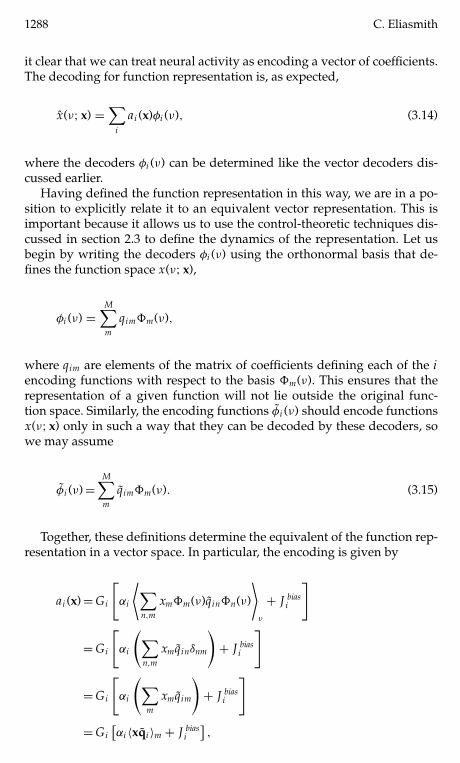
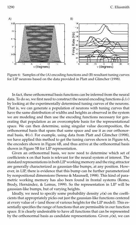
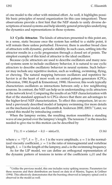
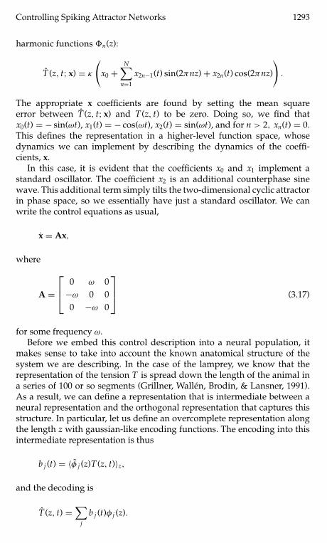
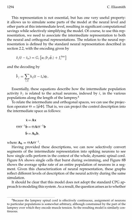
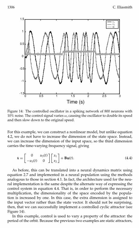
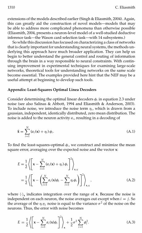Most important perhaps we describe in detail how complex control can beintegrated with standard attractor models This allows us to begin to an-swer the kinds of pressing questions now being posed by neuroscientistsincluding for example how to account for the dynamics of working mem-ory (see eg Brody Romo amp Kepecs 2003 Fuster 2001 Rainer amp Miller2002)

We briefly summarize the general framework and then demonstrate itsapplication to the construction of spiking networks that exhibit line planering cyclic and chaotic attractors Subsequently we describe how to inte-grate control signals into each of these models significantly increasing thepower and range of application of these networks

2 Framework

This section briefly summarizes the methods described in Eliasmith andAnderson (2003) which we will refer to as the neural engineering frame-work (NEF) Subsequent sections discuss the application of these methodsto the construction and control of attractor networks The following threeprinciples describe the approach

1 Neural representations are defined by the combination of nonlinearencoding (exemplified by neuron tuning curves and neural spiking)and weighted linear decoding (over populations of neurons and overtime)

2 Transformations of neural representations are functions of the vari-ables represented by neural populations Transformations are deter-mined using an alternately weighted linear decoding

3 Neural dynamics are characterized by considering neural representa-tions as control-theoretic state variables Thus the dynamics of neu-robiological systems can be analyzed using control theory

In addition to these main principles the following addendum is taken to beimportant for analyzing neural systems

Neural systems are subject to significant amounts of noise Thereforeany analysis of such systems must account for the effects of noise

Each of the next three sections describes one of the principles in the con-text of the addendum in more detail (For detailed justifications of theseprinciples see Eliasmith amp Anderson 2003) They are presented here tomake clear both the terminology and assumptions in the subsequent net-work derivations The successes of the subsequent models help to justifythe adoption of these principles

1278 C Eliasmith


ai (x) = Gi [J i (x)] (21)







x =sum

i

ai (x)φi (23)



ai (t) =sum

n


n







i

]Encoding



f (x)i to


f (x)i we



i

]Encoding


i Decoding




x(t) = Ax(t) + Bu(t) (25)


x(s) = h(s) [Ax(s) + Bu(s)]


1280 C Eliasmith




hprime(t) = 1τ

eminustτ (26)





Bprime = τB (28)




Mαβ

Mαβ

1jFβ

jFβ

iα Gi[]

Jiα(t)

synaptic weights

soma


neural description

1

sim

PSCs

dendrites

Fαβ[xβ(t)]


Σδα(t-tin)n

Σδβ

Σδβ

(t-tjn)n

(t-tjn)n

αβ

1+sτijαβ

φ

φ

φ



Fβ






1282 C Eliasmith







u(t)

x(t)

A

B

bk(t) aj(t)





x = Ax(t) + Bu(t) (31)

x(s) = 1s

[Ax(s) + Bu(s)] (32)


B prime = τ

Aprime = 1

1284 C Eliasmith

-1 -08 -06 -04 -02 0 02 04 06 08 10

50

100

150

200

250

x

Firi

ng R

ate

(Hz)


τrefj minusτRC

j ln(


)




j

](33)

and

x(t) =sum

j

a j (t)φxj (34)




]




j

] (35)


a j (t) = G j

[α j


[Aprime sum

i


k

bk(t)φuk

]rang+ J bias

j

]

(36)

= G j

[hprime(t) lowast

[sumi

ω j i ai (t) +sum

k

ω jkbk(t)

]+ J bias

j

] (37)



sumn


[sumin


sumkn


j

] (39)




dVj

dt= minus 1

τRCj

(Vj minus Rj

[sumin


sumkn


j

]) (311)


1286 C Eliasmith

0 01 02 03 04 05 06 07 08 09 1

0

1

0

1

u(t)

A)

B)

Time (s)

0

10

20

30

40

50

60

70

Neu

ron

Time (s)

C)

x(t)

-1

0 01 02 03 04 05 06 07 08 09 10 01 02 03 04 05 06 07 08 09 1












x(ν A) =Msum

m=1

xmm(ν) (312)




i

] (313)


1288 C Eliasmith


x(ν x) =sum

i

ai (x)φi (ν) (314)



φi (ν) =Msumm

qimm(ν)


φi (ν) =Msumm

qimm(ν) (315)


ai (x) = Gi

[αi

langsumnm

xmm(ν)qinn(ν)

rangν

+ J biasi

]

= Gi

[αi

(sumnm

xmqinδnm

)+ J bias

i

]

= Gi

[αi

(summ

xmqim

)+ J bias

i

]


i

]


-1 -08 -06 -04 -02 0 02 04 06 08 1

-01

0

01

ν

Φ(ν

)

Φ1Φ2Φ3Φ4Φ5

-3 -2 -1 0 1 2 3-01

0

01

ν

Φ1Φ2Φ3ΦΦ

4

5

A) B)

Φ(ν

)



x =sum

i

ai (x)qi





1290 C Eliasmith

A) B)






π

ν-π-101

0

05

1

ν0

10005001

0

05

110005001

Neuron Neuron

Tim

e (s)T

ime (s)

A) B )





1292 C Eliasmith












T(z t x) = κ

(x0 +

Nsumn=1


)



x = Ax

where

A =


(317)



b j (t) = 〈φ j (z)T(z t)〉z

and the decoding is

T(z t) =sum

j

b j (t)φ j (z)

1294 C Eliasmith



i


b j =sumin

hij(t minus tn)φi



x = Ax

minus1b = Aminus1b

b = Abb






0 05 1 15 2 25 30

05

1

15

2

25

3

35

0 05 1 15 2 250

5

10

15

20

Right side


A) B)

Firi

ng R

ate

(Hz)

Time(s)

Neu

ron

Time(s)









1296 C Eliasmith

Neuron

Neu

ron

0 20 40 60 80 1000

20

40

60

80

100






x1

x2

x3

=


x2 0 minusc

x1

x2

x3

(318)




i

] (319)


ai (x) = Gi

[sumj

(ω

ax1ij minus ω

ax2ij + ω

bx1ij minus ω

x2ij

minus ωx1x3ij + ω

x1x2ij minus ω

cx3ij

)a j (x) + J bias

i

]


x1j ω

ax2ij = αi φi1aφ

x1j ω

bx1ij = αi φi2bφ

x1j ω

x2ij = αi φi2φ

x2j


x1x3j ω

x1x2ij = αi φi3φ

x1x2j and ω



1298 C Eliasmith

0 0 5 1 1 5 2 2 5 3 3 5 4 4 5 5

-4 0

-3 0

-2 0

-1 0

0

10

20

30

40

50xyz

0 0 1 0 2 0 3 0 4 05 0 6 0 7 0 8 0 9 10

2

4

6

8

10

12

14

16

18

20

-2 0 -1 5 -10 -5 0 5 10 15 20 25

0

5

10

15

20

25

30

35

40

45

50

z

x

A)

B)

Am

plitu

deN

euro

n

Time(s)

Time(s)

C)









1300 C Eliasmith

u(t)

x(t)

Bx

A(t)

c(t)

u(t)

x(t)

Ax

Bx

A(t)

Bc

A) B)












)[

x1

x2

]= hprime(t) lowast

([x2 00 0

] [x1

x2

]+

[τ 00 τ

] [uAprime

]) (42)


p(t) =sum

i

ai (t)φpi


a j = G j

[α j


[sumi


k

bkφuk

]rang+ J bias

j

]

= G j

[sumi

ωijai (t) +sum

k


] (43)


k and


i

]


1302 C Eliasmith

0 01 02 03 04 05 06 07 08 09 1

-02

0

02

04

06

08

1

Time (s)

Con

trol

led

Filte

r

0 01 02 03 04 05 06 07 08 09 1-15

-1

-05

0

05

1

15

Inpu

t

u(t)1-A(t)

x1(t)

x2(t)

A)

B)









x(ν t + τ ) = x(ν + δ t)

=sum

m

xmeim(ν+δ)

=sum

m

xmeimνeimδ


E =

1 0 0 00 cos(mδ) sin(mδ) 0




1304 C Eliasmith








0

1

2

Tim

e (s)

πν-πLeft Right

A) B)





x =[

0 ω(t)minusω(t) 0

] [x1

x2

]+ Bu(t)

1306 C Eliasmith

0 05 1 15 2 25 3-15

-1

-05

0

05

1

15

Time (s)

x1x2ω



x =[

0 u3(t)minusu3(t) 0

] [x1

x2

]+ Bu(t) (44)







x1

x2

x3

=


=


x2 0 minusc

x1

x2

x3

+

0 0 00 0 0

minus(c + 1) 0 0

b00



1308 C Eliasmith

0 1 2 3 4 5 6 7 8 9 10-50

0

50

100

Time (s)

xyzControl

Am

plitu

de





5 Conclusion





1310 C Eliasmith





x =Nsum

i=1

(ai (x) + ηi ) φi (A1)


E = 12

lang[x minus

Nsumi=1

(ai (x) + ηi ) φi

]2rangxη

= 12

lang[x minus

(Nsum

i=1

ai (x)φi minusNsum

i=1

ηiφi

)]2rangxη

(A2)


E = 12

lang[x minus

Nsumi=1

ai (x)φi

]2rangx

+ 12σ 2

Nsumi=1

φ2i (A3)



δEδφi

= minus12

lang2

[x minus

Nsumj

a j (x)φ j

]ai (x)

rangx

+ σ 2φ jδij


Nsumj

ai (x)a j (x)φ j

rangx

+ σ 2φ jδij (A4)



(langai (x)a j (x)

rangx + σ 2δij

)φ j (A5)

or in matrix form

ϒ = φ


φ = minus1ϒ

where


rangx + σ 2δij




E = 12

lang[f (x) minus

Nsumi=1

(ai (x) + ηi ) φf (x)

i

]2rangxη



Acknowledgments


1312 C Eliasmith


References







































1314 C Eliasmith















1278 C Eliasmith


ai (x) = Gi [J i (x)] (21)







x =sum

i

ai (x)φi (23)



ai (t) =sum

n


n







i

]Encoding



f (x)i to


f (x)i we



i

]Encoding


i Decoding




x(t) = Ax(t) + Bu(t) (25)


x(s) = h(s) [Ax(s) + Bu(s)]


1280 C Eliasmith




hprime(t) = 1τ

eminustτ (26)





Bprime = τB (28)




Mαβ

Mαβ

1jFβ

jFβ

iα Gi[]

Jiα(t)

synaptic weights

soma


neural description

1

sim

PSCs

dendrites

Fαβ[xβ(t)]


Σδα(t-tin)n

Σδβ

Σδβ

(t-tjn)n

(t-tjn)n

αβ

1+sτijαβ

φ

φ

φ



Fβ






1282 C Eliasmith







u(t)

x(t)

A

B

bk(t) aj(t)





x = Ax(t) + Bu(t) (31)

x(s) = 1s

[Ax(s) + Bu(s)] (32)


B prime = τ

Aprime = 1

1284 C Eliasmith

-1 -08 -06 -04 -02 0 02 04 06 08 10

50

100

150

200

250

x

Firi

ng R

ate

(Hz)


τrefj minusτRC

j ln(


)




j

](33)

and

x(t) =sum

j

a j (t)φxj (34)




]




j

] (35)


a j (t) = G j

[α j


[Aprime sum

i


k

bk(t)φuk

]rang+ J bias

j

]

(36)

= G j

[hprime(t) lowast

[sumi

ω j i ai (t) +sum

k

ω jkbk(t)

]+ J bias

j

] (37)



sumn


[sumin


sumkn


j

] (39)




dVj

dt= minus 1

τRCj

(Vj minus Rj

[sumin


sumkn


j

]) (311)


1286 C Eliasmith

0 01 02 03 04 05 06 07 08 09 1

0

1

0

1

u(t)

A)

B)

Time (s)

0

10

20

30

40

50

60

70

Neu

ron

Time (s)

C)

x(t)

-1

0 01 02 03 04 05 06 07 08 09 10 01 02 03 04 05 06 07 08 09 1












x(ν A) =Msum

m=1

xmm(ν) (312)




i

] (313)


1288 C Eliasmith


x(ν x) =sum

i

ai (x)φi (ν) (314)



φi (ν) =Msumm

qimm(ν)


φi (ν) =Msumm

qimm(ν) (315)


ai (x) = Gi

[αi

langsumnm

xmm(ν)qinn(ν)

rangν

+ J biasi

]

= Gi

[αi

(sumnm

xmqinδnm

)+ J bias

i

]

= Gi

[αi

(summ

xmqim

)+ J bias

i

]


i

]


-1 -08 -06 -04 -02 0 02 04 06 08 1

-01

0

01

ν

Φ(ν

)

Φ1Φ2Φ3Φ4Φ5

-3 -2 -1 0 1 2 3-01

0

01

ν

Φ1Φ2Φ3ΦΦ

4

5

A) B)

Φ(ν

)



x =sum

i

ai (x)qi





1290 C Eliasmith

A) B)






π

ν-π-101

0

05

1

ν0

10005001

0

05

110005001

Neuron Neuron

Tim

e (s)T

ime (s)

A) B )





1292 C Eliasmith












T(z t x) = κ

(x0 +

Nsumn=1


)



x = Ax

where

A =


(317)



b j (t) = 〈φ j (z)T(z t)〉z

and the decoding is

T(z t) =sum

j

b j (t)φ j (z)

1294 C Eliasmith



i


b j =sumin

hij(t minus tn)φi



x = Ax

minus1b = Aminus1b

b = Abb






0 05 1 15 2 25 30

05

1

15

2

25

3

35

0 05 1 15 2 250

5

10

15

20

Right side


A) B)

Firi

ng R

ate

(Hz)

Time(s)

Neu

ron

Time(s)









1296 C Eliasmith

Neuron

Neu

ron

0 20 40 60 80 1000

20

40

60

80

100






x1

x2

x3

=


x2 0 minusc

x1

x2

x3

(318)




i

] (319)


ai (x) = Gi

[sumj

(ω

ax1ij minus ω

ax2ij + ω

bx1ij minus ω

x2ij

minus ωx1x3ij + ω

x1x2ij minus ω

cx3ij

)a j (x) + J bias

i

]


x1j ω

ax2ij = αi φi1aφ

x1j ω

bx1ij = αi φi2bφ

x1j ω

x2ij = αi φi2φ

x2j


x1x3j ω

x1x2ij = αi φi3φ

x1x2j and ω



1298 C Eliasmith

0 0 5 1 1 5 2 2 5 3 3 5 4 4 5 5

-4 0

-3 0

-2 0

-1 0

0

10

20

30

40

50xyz

0 0 1 0 2 0 3 0 4 05 0 6 0 7 0 8 0 9 10

2

4

6

8

10

12

14

16

18

20

-2 0 -1 5 -10 -5 0 5 10 15 20 25

0

5

10

15

20

25

30

35

40

45

50

z

x

A)

B)

Am

plitu

deN

euro

n

Time(s)

Time(s)

C)









1300 C Eliasmith

u(t)

x(t)

Bx

A(t)

c(t)

u(t)

x(t)

Ax

Bx

A(t)

Bc

A) B)












)[

x1

x2

]= hprime(t) lowast

([x2 00 0

] [x1

x2

]+

[τ 00 τ

] [uAprime

]) (42)


p(t) =sum

i

ai (t)φpi


a j = G j

[α j


[sumi


k

bkφuk

]rang+ J bias

j

]

= G j

[sumi

ωijai (t) +sum

k


] (43)


k and


i

]


1302 C Eliasmith

0 01 02 03 04 05 06 07 08 09 1

-02

0

02

04

06

08

1

Time (s)

Con

trol

led

Filte

r

0 01 02 03 04 05 06 07 08 09 1-15

-1

-05

0

05

1

15

Inpu

t

u(t)1-A(t)

x1(t)

x2(t)

A)

B)









x(ν t + τ ) = x(ν + δ t)

=sum

m

xmeim(ν+δ)

=sum

m

xmeimνeimδ


E =

1 0 0 00 cos(mδ) sin(mδ) 0




1304 C Eliasmith








0

1

2

Tim

e (s)

πν-πLeft Right

A) B)





x =[

0 ω(t)minusω(t) 0

] [x1

x2

]+ Bu(t)

1306 C Eliasmith

0 05 1 15 2 25 3-15

-1

-05

0

05

1

15

Time (s)

x1x2ω



x =[

0 u3(t)minusu3(t) 0

] [x1

x2

]+ Bu(t) (44)







x1

x2

x3

=


=


x2 0 minusc

x1

x2

x3

+

0 0 00 0 0

minus(c + 1) 0 0

b00



1308 C Eliasmith

0 1 2 3 4 5 6 7 8 9 10-50

0

50

100

Time (s)

xyzControl

Am

plitu

de





5 Conclusion





1310 C Eliasmith





x =Nsum

i=1

(ai (x) + ηi ) φi (A1)


E = 12

lang[x minus

Nsumi=1

(ai (x) + ηi ) φi

]2rangxη

= 12

lang[x minus

(Nsum

i=1

ai (x)φi minusNsum

i=1

ηiφi

)]2rangxη

(A2)


E = 12

lang[x minus

Nsumi=1

ai (x)φi

]2rangx

+ 12σ 2

Nsumi=1

φ2i (A3)



δEδφi

= minus12

lang2

[x minus

Nsumj

a j (x)φ j

]ai (x)

rangx

+ σ 2φ jδij


Nsumj

ai (x)a j (x)φ j

rangx

+ σ 2φ jδij (A4)



(langai (x)a j (x)

rangx + σ 2δij

)φ j (A5)

or in matrix form

ϒ = φ


φ = minus1ϒ

where


rangx + σ 2δij




E = 12

lang[f (x) minus

Nsumi=1

(ai (x) + ηi ) φf (x)

i

]2rangxη



Acknowledgments


1312 C Eliasmith


References







































1314 C Eliasmith



















i

]Encoding



f (x)i to


f (x)i we



i

]Encoding


i Decoding




x(t) = Ax(t) + Bu(t) (25)


x(s) = h(s) [Ax(s) + Bu(s)]


1280 C Eliasmith




hprime(t) = 1τ

eminustτ (26)





Bprime = τB (28)




Mαβ

Mαβ

1jFβ

jFβ

iα Gi[]

Jiα(t)

synaptic weights

soma


neural description

1

sim

PSCs

dendrites

Fαβ[xβ(t)]


Σδα(t-tin)n

Σδβ

Σδβ

(t-tjn)n

(t-tjn)n

αβ

1+sτijαβ

φ

φ

φ



Fβ






1282 C Eliasmith







u(t)

x(t)

A

B

bk(t) aj(t)





x = Ax(t) + Bu(t) (31)

x(s) = 1s

[Ax(s) + Bu(s)] (32)


B prime = τ

Aprime = 1

1284 C Eliasmith

-1 -08 -06 -04 -02 0 02 04 06 08 10

50

100

150

200

250

x

Firi

ng R

ate

(Hz)


τrefj minusτRC

j ln(


)




j

](33)

and

x(t) =sum

j

a j (t)φxj (34)




]




j

] (35)


a j (t) = G j

[α j


[Aprime sum

i


k

bk(t)φuk

]rang+ J bias

j

]

(36)

= G j

[hprime(t) lowast

[sumi

ω j i ai (t) +sum

k

ω jkbk(t)

]+ J bias

j

] (37)



sumn


[sumin


sumkn


j

] (39)




dVj

dt= minus 1

τRCj

(Vj minus Rj

[sumin


sumkn


j

]) (311)


1286 C Eliasmith

0 01 02 03 04 05 06 07 08 09 1

0

1

0

1

u(t)

A)

B)

Time (s)

0

10

20

30

40

50

60

70

Neu

ron

Time (s)

C)

x(t)

-1

0 01 02 03 04 05 06 07 08 09 10 01 02 03 04 05 06 07 08 09 1












x(ν A) =Msum

m=1

xmm(ν) (312)




i

] (313)


1288 C Eliasmith


x(ν x) =sum

i

ai (x)φi (ν) (314)



φi (ν) =Msumm

qimm(ν)


φi (ν) =Msumm

qimm(ν) (315)


ai (x) = Gi

[αi

langsumnm

xmm(ν)qinn(ν)

rangν

+ J biasi

]

= Gi

[αi

(sumnm

xmqinδnm

)+ J bias

i

]

= Gi

[αi

(summ

xmqim

)+ J bias

i

]


i

]


-1 -08 -06 -04 -02 0 02 04 06 08 1

-01

0

01

ν

Φ(ν

)

Φ1Φ2Φ3Φ4Φ5

-3 -2 -1 0 1 2 3-01

0

01

ν

Φ1Φ2Φ3ΦΦ

4

5

A) B)

Φ(ν

)



x =sum

i

ai (x)qi





1290 C Eliasmith

A) B)






π

ν-π-101

0

05

1

ν0

10005001

0

05

110005001

Neuron Neuron

Tim

e (s)T

ime (s)

A) B )





1292 C Eliasmith












T(z t x) = κ

(x0 +

Nsumn=1


)



x = Ax

where

A =


(317)



b j (t) = 〈φ j (z)T(z t)〉z

and the decoding is

T(z t) =sum

j

b j (t)φ j (z)

1294 C Eliasmith



i


b j =sumin

hij(t minus tn)φi



x = Ax

minus1b = Aminus1b

b = Abb






0 05 1 15 2 25 30

05

1

15

2

25

3

35

0 05 1 15 2 250

5

10

15

20

Right side


A) B)

Firi

ng R

ate

(Hz)

Time(s)

Neu

ron

Time(s)









1296 C Eliasmith

Neuron

Neu

ron

0 20 40 60 80 1000

20

40

60

80

100






x1

x2

x3

=


x2 0 minusc

x1

x2

x3

(318)




i

] (319)


ai (x) = Gi

[sumj

(ω

ax1ij minus ω

ax2ij + ω

bx1ij minus ω

x2ij

minus ωx1x3ij + ω

x1x2ij minus ω

cx3ij

)a j (x) + J bias

i

]


x1j ω

ax2ij = αi φi1aφ

x1j ω

bx1ij = αi φi2bφ

x1j ω

x2ij = αi φi2φ

x2j


x1x3j ω

x1x2ij = αi φi3φ

x1x2j and ω



1298 C Eliasmith

0 0 5 1 1 5 2 2 5 3 3 5 4 4 5 5

-4 0

-3 0

-2 0

-1 0

0

10

20

30

40

50xyz

0 0 1 0 2 0 3 0 4 05 0 6 0 7 0 8 0 9 10

2

4

6

8

10

12

14

16

18

20

-2 0 -1 5 -10 -5 0 5 10 15 20 25

0

5

10

15

20

25

30

35

40

45

50

z

x

A)

B)

Am

plitu

deN

euro

n

Time(s)

Time(s)

C)









1300 C Eliasmith

u(t)

x(t)

Bx

A(t)

c(t)

u(t)

x(t)

Ax

Bx

A(t)

Bc

A) B)












)[

x1

x2

]= hprime(t) lowast

([x2 00 0

] [x1

x2

]+

[τ 00 τ

] [uAprime

]) (42)


p(t) =sum

i

ai (t)φpi


a j = G j

[α j


[sumi


k

bkφuk

]rang+ J bias

j

]

= G j

[sumi

ωijai (t) +sum

k


] (43)


k and


i

]


1302 C Eliasmith

0 01 02 03 04 05 06 07 08 09 1

-02

0

02

04

06

08

1

Time (s)

Con

trol

led

Filte

r

0 01 02 03 04 05 06 07 08 09 1-15

-1

-05

0

05

1

15

Inpu

t

u(t)1-A(t)

x1(t)

x2(t)

A)

B)









x(ν t + τ ) = x(ν + δ t)

=sum

m

xmeim(ν+δ)

=sum

m

xmeimνeimδ


E =

1 0 0 00 cos(mδ) sin(mδ) 0




1304 C Eliasmith








0

1

2

Tim

e (s)

πν-πLeft Right

A) B)





x =[

0 ω(t)minusω(t) 0

] [x1

x2

]+ Bu(t)

1306 C Eliasmith

0 05 1 15 2 25 3-15

-1

-05

0

05

1

15

Time (s)

x1x2ω



x =[

0 u3(t)minusu3(t) 0

] [x1

x2

]+ Bu(t) (44)







x1

x2

x3

=


=


x2 0 minusc

x1

x2

x3

+

0 0 00 0 0

minus(c + 1) 0 0

b00



1308 C Eliasmith

0 1 2 3 4 5 6 7 8 9 10-50

0

50

100

Time (s)

xyzControl

Am

plitu

de





5 Conclusion





1310 C Eliasmith





x =Nsum

i=1

(ai (x) + ηi ) φi (A1)


E = 12

lang[x minus

Nsumi=1

(ai (x) + ηi ) φi

]2rangxη

= 12

lang[x minus

(Nsum

i=1

ai (x)φi minusNsum

i=1

ηiφi

)]2rangxη

(A2)


E = 12

lang[x minus

Nsumi=1

ai (x)φi

]2rangx

+ 12σ 2

Nsumi=1

φ2i (A3)



δEδφi

= minus12

lang2

[x minus

Nsumj

a j (x)φ j

]ai (x)

rangx

+ σ 2φ jδij


Nsumj

ai (x)a j (x)φ j

rangx

+ σ 2φ jδij (A4)



(langai (x)a j (x)

rangx + σ 2δij

)φ j (A5)

or in matrix form

ϒ = φ


φ = minus1ϒ

where


rangx + σ 2δij




E = 12

lang[f (x) minus

Nsumi=1

(ai (x) + ηi ) φf (x)

i

]2rangxη



Acknowledgments


1312 C Eliasmith


References







































1314 C Eliasmith















1280 C Eliasmith




hprime(t) = 1τ

eminustτ (26)





Bprime = τB (28)




Mαβ

Mαβ

1jFβ

jFβ

iα Gi[]

Jiα(t)

synaptic weights

soma


neural description

1

sim

PSCs

dendrites

Fαβ[xβ(t)]


Σδα(t-tin)n

Σδβ

Σδβ

(t-tjn)n

(t-tjn)n

αβ

1+sτijαβ

φ

φ

φ



Fβ






1282 C Eliasmith







u(t)

x(t)

A

B

bk(t) aj(t)





x = Ax(t) + Bu(t) (31)

x(s) = 1s

[Ax(s) + Bu(s)] (32)


B prime = τ

Aprime = 1

1284 C Eliasmith

-1 -08 -06 -04 -02 0 02 04 06 08 10

50

100

150

200

250

x

Firi

ng R

ate

(Hz)


τrefj minusτRC

j ln(


)




j

](33)

and

x(t) =sum

j

a j (t)φxj (34)




]




j

] (35)


a j (t) = G j

[α j


[Aprime sum

i


k

bk(t)φuk

]rang+ J bias

j

]

(36)

= G j

[hprime(t) lowast

[sumi

ω j i ai (t) +sum

k

ω jkbk(t)

]+ J bias

j

] (37)



sumn


[sumin


sumkn


j

] (39)




dVj

dt= minus 1

τRCj

(Vj minus Rj

[sumin


sumkn


j

]) (311)


1286 C Eliasmith

0 01 02 03 04 05 06 07 08 09 1

0

1

0

1

u(t)

A)

B)

Time (s)

0

10

20

30

40

50

60

70

Neu

ron

Time (s)

C)

x(t)

-1

0 01 02 03 04 05 06 07 08 09 10 01 02 03 04 05 06 07 08 09 1












x(ν A) =Msum

m=1

xmm(ν) (312)




i

] (313)


1288 C Eliasmith


x(ν x) =sum

i

ai (x)φi (ν) (314)



φi (ν) =Msumm

qimm(ν)


φi (ν) =Msumm

qimm(ν) (315)


ai (x) = Gi

[αi

langsumnm

xmm(ν)qinn(ν)

rangν

+ J biasi

]

= Gi

[αi

(sumnm

xmqinδnm

)+ J bias

i

]

= Gi

[αi

(summ

xmqim

)+ J bias

i

]


i

]


-1 -08 -06 -04 -02 0 02 04 06 08 1

-01

0

01

ν

Φ(ν

)

Φ1Φ2Φ3Φ4Φ5

-3 -2 -1 0 1 2 3-01

0

01

ν

Φ1Φ2Φ3ΦΦ

4

5

A) B)

Φ(ν

)



x =sum

i

ai (x)qi





1290 C Eliasmith

A) B)






π

ν-π-101

0

05

1

ν0

10005001

0

05

110005001

Neuron Neuron

Tim

e (s)T

ime (s)

A) B )





1292 C Eliasmith












T(z t x) = κ

(x0 +

Nsumn=1


)



x = Ax

where

A =


(317)



b j (t) = 〈φ j (z)T(z t)〉z

and the decoding is

T(z t) =sum

j

b j (t)φ j (z)

1294 C Eliasmith



i


b j =sumin

hij(t minus tn)φi



x = Ax

minus1b = Aminus1b

b = Abb






0 05 1 15 2 25 30

05

1

15

2

25

3

35

0 05 1 15 2 250

5

10

15

20

Right side


A) B)

Firi

ng R

ate

(Hz)

Time(s)

Neu

ron

Time(s)









1296 C Eliasmith

Neuron

Neu

ron

0 20 40 60 80 1000

20

40

60

80

100






x1

x2

x3

=


x2 0 minusc

x1

x2

x3

(318)




i

] (319)


ai (x) = Gi

[sumj

(ω

ax1ij minus ω

ax2ij + ω

bx1ij minus ω

x2ij

minus ωx1x3ij + ω

x1x2ij minus ω

cx3ij

)a j (x) + J bias

i

]


x1j ω

ax2ij = αi φi1aφ

x1j ω

bx1ij = αi φi2bφ

x1j ω

x2ij = αi φi2φ

x2j


x1x3j ω

x1x2ij = αi φi3φ

x1x2j and ω



1298 C Eliasmith

0 0 5 1 1 5 2 2 5 3 3 5 4 4 5 5

-4 0

-3 0

-2 0

-1 0

0

10

20

30

40

50xyz

0 0 1 0 2 0 3 0 4 05 0 6 0 7 0 8 0 9 10

2

4

6

8

10

12

14

16

18

20

-2 0 -1 5 -10 -5 0 5 10 15 20 25

0

5

10

15

20

25

30

35

40

45

50

z

x

A)

B)

Am

plitu

deN

euro

n

Time(s)

Time(s)

C)









1300 C Eliasmith

u(t)

x(t)

Bx

A(t)

c(t)

u(t)

x(t)

Ax

Bx

A(t)

Bc

A) B)












)[

x1

x2

]= hprime(t) lowast

([x2 00 0

] [x1

x2

]+

[τ 00 τ

] [uAprime

]) (42)


p(t) =sum

i

ai (t)φpi


a j = G j

[α j


[sumi


k

bkφuk

]rang+ J bias

j

]

= G j

[sumi

ωijai (t) +sum

k


] (43)


k and


i

]


1302 C Eliasmith

0 01 02 03 04 05 06 07 08 09 1

-02

0

02

04

06

08

1

Time (s)

Con

trol

led

Filte

r

0 01 02 03 04 05 06 07 08 09 1-15

-1

-05

0

05

1

15

Inpu

t

u(t)1-A(t)

x1(t)

x2(t)

A)

B)









x(ν t + τ ) = x(ν + δ t)

=sum

m

xmeim(ν+δ)

=sum

m

xmeimνeimδ


E =

1 0 0 00 cos(mδ) sin(mδ) 0




1304 C Eliasmith








0

1

2

Tim

e (s)

πν-πLeft Right

A) B)





x =[

0 ω(t)minusω(t) 0

] [x1

x2

]+ Bu(t)

1306 C Eliasmith

0 05 1 15 2 25 3-15

-1

-05

0

05

1

15

Time (s)

x1x2ω



x =[

0 u3(t)minusu3(t) 0

] [x1

x2

]+ Bu(t) (44)







x1

x2

x3

=


=


x2 0 minusc

x1

x2

x3

+

0 0 00 0 0

minus(c + 1) 0 0

b00



1308 C Eliasmith

0 1 2 3 4 5 6 7 8 9 10-50

0

50

100

Time (s)

xyzControl

Am

plitu

de





5 Conclusion





1310 C Eliasmith





x =Nsum

i=1

(ai (x) + ηi ) φi (A1)


E = 12

lang[x minus

Nsumi=1

(ai (x) + ηi ) φi

]2rangxη

= 12

lang[x minus

(Nsum

i=1

ai (x)φi minusNsum

i=1

ηiφi

)]2rangxη

(A2)


E = 12

lang[x minus

Nsumi=1

ai (x)φi

]2rangx

+ 12σ 2

Nsumi=1

φ2i (A3)



δEδφi

= minus12

lang2

[x minus

Nsumj

a j (x)φ j

]ai (x)

rangx

+ σ 2φ jδij


Nsumj

ai (x)a j (x)φ j

rangx

+ σ 2φ jδij (A4)



(langai (x)a j (x)

rangx + σ 2δij

)φ j (A5)

or in matrix form

ϒ = φ


φ = minus1ϒ

where


rangx + σ 2δij




E = 12

lang[f (x) minus

Nsumi=1

(ai (x) + ηi ) φf (x)

i

]2rangxη



Acknowledgments


1312 C Eliasmith


References







































1314 C Eliasmith
















Mαβ

Mαβ

1jFβ

jFβ

iα Gi[]

Jiα(t)

synaptic weights

soma


neural description

1

sim

PSCs

dendrites

Fαβ[xβ(t)]


Σδα(t-tin)n

Σδβ

Σδβ

(t-tjn)n

(t-tjn)n

αβ

1+sτijαβ

φ

φ

φ



Fβ






1282 C Eliasmith







u(t)

x(t)

A

B

bk(t) aj(t)





x = Ax(t) + Bu(t) (31)

x(s) = 1s

[Ax(s) + Bu(s)] (32)


B prime = τ

Aprime = 1

1284 C Eliasmith

-1 -08 -06 -04 -02 0 02 04 06 08 10

50

100

150

200

250

x

Firi

ng R

ate

(Hz)


τrefj minusτRC

j ln(


)




j

](33)

and

x(t) =sum

j

a j (t)φxj (34)




]




j

] (35)


a j (t) = G j

[α j


[Aprime sum

i


k

bk(t)φuk

]rang+ J bias

j

]

(36)

= G j

[hprime(t) lowast

[sumi

ω j i ai (t) +sum

k

ω jkbk(t)

]+ J bias

j

] (37)



sumn


[sumin


sumkn


j

] (39)




dVj

dt= minus 1

τRCj

(Vj minus Rj

[sumin


sumkn


j

]) (311)


1286 C Eliasmith

0 01 02 03 04 05 06 07 08 09 1

0

1

0

1

u(t)

A)

B)

Time (s)

0

10

20

30

40

50

60

70

Neu

ron

Time (s)

C)

x(t)

-1

0 01 02 03 04 05 06 07 08 09 10 01 02 03 04 05 06 07 08 09 1












x(ν A) =Msum

m=1

xmm(ν) (312)




i

] (313)


1288 C Eliasmith


x(ν x) =sum

i

ai (x)φi (ν) (314)



φi (ν) =Msumm

qimm(ν)


φi (ν) =Msumm

qimm(ν) (315)


ai (x) = Gi

[αi

langsumnm

xmm(ν)qinn(ν)

rangν

+ J biasi

]

= Gi

[αi

(sumnm

xmqinδnm

)+ J bias

i

]

= Gi

[αi

(summ

xmqim

)+ J bias

i

]


i

]


-1 -08 -06 -04 -02 0 02 04 06 08 1

-01

0

01

ν

Φ(ν

)

Φ1Φ2Φ3Φ4Φ5

-3 -2 -1 0 1 2 3-01

0

01

ν

Φ1Φ2Φ3ΦΦ

4

5

A) B)

Φ(ν

)



x =sum

i

ai (x)qi





1290 C Eliasmith

A) B)






π

ν-π-101

0

05

1

ν0

10005001

0

05

110005001

Neuron Neuron

Tim

e (s)T

ime (s)

A) B )





1292 C Eliasmith












T(z t x) = κ

(x0 +

Nsumn=1


)



x = Ax

where

A =


(317)



b j (t) = 〈φ j (z)T(z t)〉z

and the decoding is

T(z t) =sum

j

b j (t)φ j (z)

1294 C Eliasmith



i


b j =sumin

hij(t minus tn)φi



x = Ax

minus1b = Aminus1b

b = Abb






0 05 1 15 2 25 30

05

1

15

2

25

3

35

0 05 1 15 2 250

5

10

15

20

Right side


A) B)

Firi

ng R

ate

(Hz)

Time(s)

Neu

ron

Time(s)









1296 C Eliasmith

Neuron

Neu

ron

0 20 40 60 80 1000

20

40

60

80

100






x1

x2

x3

=


x2 0 minusc

x1

x2

x3

(318)




i

] (319)


ai (x) = Gi

[sumj

(ω

ax1ij minus ω

ax2ij + ω

bx1ij minus ω

x2ij

minus ωx1x3ij + ω

x1x2ij minus ω

cx3ij

)a j (x) + J bias

i

]


x1j ω

ax2ij = αi φi1aφ

x1j ω

bx1ij = αi φi2bφ

x1j ω

x2ij = αi φi2φ

x2j


x1x3j ω

x1x2ij = αi φi3φ

x1x2j and ω



1298 C Eliasmith

0 0 5 1 1 5 2 2 5 3 3 5 4 4 5 5

-4 0

-3 0

-2 0

-1 0

0

10

20

30

40

50xyz

0 0 1 0 2 0 3 0 4 05 0 6 0 7 0 8 0 9 10

2

4

6

8

10

12

14

16

18

20

-2 0 -1 5 -10 -5 0 5 10 15 20 25

0

5

10

15

20

25

30

35

40

45

50

z

x

A)

B)

Am

plitu

deN

euro

n

Time(s)

Time(s)

C)









1300 C Eliasmith

u(t)

x(t)

Bx

A(t)

c(t)

u(t)

x(t)

Ax

Bx

A(t)

Bc

A) B)












)[

x1

x2

]= hprime(t) lowast

([x2 00 0

] [x1

x2

]+

[τ 00 τ

] [uAprime

]) (42)


p(t) =sum

i

ai (t)φpi


a j = G j

[α j


[sumi


k

bkφuk

]rang+ J bias

j

]

= G j

[sumi

ωijai (t) +sum

k


] (43)


k and


i

]


1302 C Eliasmith

0 01 02 03 04 05 06 07 08 09 1

-02

0

02

04

06

08

1

Time (s)

Con

trol

led

Filte

r

0 01 02 03 04 05 06 07 08 09 1-15

-1

-05

0

05

1

15

Inpu

t

u(t)1-A(t)

x1(t)

x2(t)

A)

B)









x(ν t + τ ) = x(ν + δ t)

=sum

m

xmeim(ν+δ)

=sum

m

xmeimνeimδ


E =

1 0 0 00 cos(mδ) sin(mδ) 0




1304 C Eliasmith








0

1

2

Tim

e (s)

πν-πLeft Right

A) B)





x =[

0 ω(t)minusω(t) 0

] [x1

x2

]+ Bu(t)

1306 C Eliasmith

0 05 1 15 2 25 3-15

-1

-05

0

05

1

15

Time (s)

x1x2ω



x =[

0 u3(t)minusu3(t) 0

] [x1

x2

]+ Bu(t) (44)







x1

x2

x3

=


=


x2 0 minusc

x1

x2

x3

+

0 0 00 0 0

minus(c + 1) 0 0

b00



1308 C Eliasmith

0 1 2 3 4 5 6 7 8 9 10-50

0

50

100

Time (s)

xyzControl

Am

plitu

de





5 Conclusion





1310 C Eliasmith





x =Nsum

i=1

(ai (x) + ηi ) φi (A1)


E = 12

lang[x minus

Nsumi=1

(ai (x) + ηi ) φi

]2rangxη

= 12

lang[x minus

(Nsum

i=1

ai (x)φi minusNsum

i=1

ηiφi

)]2rangxη

(A2)


E = 12

lang[x minus

Nsumi=1

ai (x)φi

]2rangx

+ 12σ 2

Nsumi=1

φ2i (A3)



δEδφi

= minus12

lang2

[x minus

Nsumj

a j (x)φ j

]ai (x)

rangx

+ σ 2φ jδij


Nsumj

ai (x)a j (x)φ j

rangx

+ σ 2φ jδij (A4)



(langai (x)a j (x)

rangx + σ 2δij

)φ j (A5)

or in matrix form

ϒ = φ


φ = minus1ϒ

where


rangx + σ 2δij




E = 12

lang[f (x) minus

Nsumi=1

(ai (x) + ηi ) φf (x)

i

]2rangxη



Acknowledgments


1312 C Eliasmith


References







































1314 C Eliasmith















1282 C Eliasmith







u(t)

x(t)

A

B

bk(t) aj(t)





x = Ax(t) + Bu(t) (31)

x(s) = 1s

[Ax(s) + Bu(s)] (32)


B prime = τ

Aprime = 1

1284 C Eliasmith

-1 -08 -06 -04 -02 0 02 04 06 08 10

50

100

150

200

250

x

Firi

ng R

ate

(Hz)


τrefj minusτRC

j ln(


)




j

](33)

and

x(t) =sum

j

a j (t)φxj (34)




]




j

] (35)


a j (t) = G j

[α j


[Aprime sum

i


k

bk(t)φuk

]rang+ J bias

j

]

(36)

= G j

[hprime(t) lowast

[sumi

ω j i ai (t) +sum

k

ω jkbk(t)

]+ J bias

j

] (37)



sumn


[sumin


sumkn


j

] (39)




dVj

dt= minus 1

τRCj

(Vj minus Rj

[sumin


sumkn


j

]) (311)


1286 C Eliasmith

0 01 02 03 04 05 06 07 08 09 1

0

1

0

1

u(t)

A)

B)

Time (s)

0

10

20

30

40

50

60

70

Neu

ron

Time (s)

C)

x(t)

-1

0 01 02 03 04 05 06 07 08 09 10 01 02 03 04 05 06 07 08 09 1












x(ν A) =Msum

m=1

xmm(ν) (312)




i

] (313)


1288 C Eliasmith


x(ν x) =sum

i

ai (x)φi (ν) (314)



φi (ν) =Msumm

qimm(ν)


φi (ν) =Msumm

qimm(ν) (315)


ai (x) = Gi

[αi

langsumnm

xmm(ν)qinn(ν)

rangν

+ J biasi

]

= Gi

[αi

(sumnm

xmqinδnm

)+ J bias

i

]

= Gi

[αi

(summ

xmqim

)+ J bias

i

]


i

]


-1 -08 -06 -04 -02 0 02 04 06 08 1

-01

0

01

ν

Φ(ν

)

Φ1Φ2Φ3Φ4Φ5

-3 -2 -1 0 1 2 3-01

0

01

ν

Φ1Φ2Φ3ΦΦ

4

5

A) B)

Φ(ν

)



x =sum

i

ai (x)qi





1290 C Eliasmith

A) B)






π

ν-π-101

0

05

1

ν0

10005001

0

05

110005001

Neuron Neuron

Tim

e (s)T

ime (s)

A) B )





1292 C Eliasmith












T(z t x) = κ

(x0 +

Nsumn=1


)



x = Ax

where

A =


(317)



b j (t) = 〈φ j (z)T(z t)〉z

and the decoding is

T(z t) =sum

j

b j (t)φ j (z)

1294 C Eliasmith



i


b j =sumin

hij(t minus tn)φi



x = Ax

minus1b = Aminus1b

b = Abb






0 05 1 15 2 25 30

05

1

15

2

25

3

35

0 05 1 15 2 250

5

10

15

20

Right side


A) B)

Firi

ng R

ate

(Hz)

Time(s)

Neu

ron

Time(s)









1296 C Eliasmith

Neuron

Neu

ron

0 20 40 60 80 1000

20

40

60

80

100






x1

x2

x3

=


x2 0 minusc

x1

x2

x3

(318)




i

] (319)


ai (x) = Gi

[sumj

(ω

ax1ij minus ω

ax2ij + ω

bx1ij minus ω

x2ij

minus ωx1x3ij + ω

x1x2ij minus ω

cx3ij

)a j (x) + J bias

i

]


x1j ω

ax2ij = αi φi1aφ

x1j ω

bx1ij = αi φi2bφ

x1j ω

x2ij = αi φi2φ

x2j


x1x3j ω

x1x2ij = αi φi3φ

x1x2j and ω



1298 C Eliasmith

0 0 5 1 1 5 2 2 5 3 3 5 4 4 5 5

-4 0

-3 0

-2 0

-1 0

0

10

20

30

40

50xyz

0 0 1 0 2 0 3 0 4 05 0 6 0 7 0 8 0 9 10

2

4

6

8

10

12

14

16

18

20

-2 0 -1 5 -10 -5 0 5 10 15 20 25

0

5

10

15

20

25

30

35

40

45

50

z

x

A)

B)

Am

plitu

deN

euro

n

Time(s)

Time(s)

C)









1300 C Eliasmith

u(t)

x(t)

Bx

A(t)

c(t)

u(t)

x(t)

Ax

Bx

A(t)

Bc

A) B)












)[

x1

x2

]= hprime(t) lowast

([x2 00 0

] [x1

x2

]+

[τ 00 τ

] [uAprime

]) (42)


p(t) =sum

i

ai (t)φpi


a j = G j

[α j


[sumi


k

bkφuk

]rang+ J bias

j

]

= G j

[sumi

ωijai (t) +sum

k


] (43)


k and


i

]


1302 C Eliasmith

0 01 02 03 04 05 06 07 08 09 1

-02

0

02

04

06

08

1

Time (s)

Con

trol

led

Filte

r

0 01 02 03 04 05 06 07 08 09 1-15

-1

-05

0

05

1

15

Inpu

t

u(t)1-A(t)

x1(t)

x2(t)

A)

B)









x(ν t + τ ) = x(ν + δ t)

=sum

m

xmeim(ν+δ)

=sum

m

xmeimνeimδ


E =

1 0 0 00 cos(mδ) sin(mδ) 0




1304 C Eliasmith








0

1

2

Tim

e (s)

πν-πLeft Right

A) B)





x =[

0 ω(t)minusω(t) 0

] [x1

x2

]+ Bu(t)

1306 C Eliasmith

0 05 1 15 2 25 3-15

-1

-05

0

05

1

15

Time (s)

x1x2ω



x =[

0 u3(t)minusu3(t) 0

] [x1

x2

]+ Bu(t) (44)







x1

x2

x3

=


=


x2 0 minusc

x1

x2

x3

+

0 0 00 0 0

minus(c + 1) 0 0

b00



1308 C Eliasmith

0 1 2 3 4 5 6 7 8 9 10-50

0

50

100

Time (s)

xyzControl

Am

plitu

de





5 Conclusion





1310 C Eliasmith





x =Nsum

i=1

(ai (x) + ηi ) φi (A1)


E = 12

lang[x minus

Nsumi=1

(ai (x) + ηi ) φi

]2rangxη

= 12

lang[x minus

(Nsum

i=1

ai (x)φi minusNsum

i=1

ηiφi

)]2rangxη

(A2)


E = 12

lang[x minus

Nsumi=1

ai (x)φi

]2rangx

+ 12σ 2

Nsumi=1

φ2i (A3)



δEδφi

= minus12

lang2

[x minus

Nsumj

a j (x)φ j

]ai (x)

rangx

+ σ 2φ jδij


Nsumj

ai (x)a j (x)φ j

rangx

+ σ 2φ jδij (A4)



(langai (x)a j (x)

rangx + σ 2δij

)φ j (A5)

or in matrix form

ϒ = φ


φ = minus1ϒ

where


rangx + σ 2δij




E = 12

lang[f (x) minus

Nsumi=1

(ai (x) + ηi ) φf (x)

i

]2rangxη



Acknowledgments


1312 C Eliasmith


References







































1314 C Eliasmith
















u(t)

x(t)

A

B

bk(t) aj(t)





x = Ax(t) + Bu(t) (31)

x(s) = 1s

[Ax(s) + Bu(s)] (32)


B prime = τ

Aprime = 1

1284 C Eliasmith

-1 -08 -06 -04 -02 0 02 04 06 08 10

50

100

150

200

250

x

Firi

ng R

ate

(Hz)


τrefj minusτRC

j ln(


)




j

](33)

and

x(t) =sum

j

a j (t)φxj (34)




]




j

] (35)


a j (t) = G j

[α j


[Aprime sum

i


k

bk(t)φuk

]rang+ J bias

j

]

(36)

= G j

[hprime(t) lowast

[sumi

ω j i ai (t) +sum

k

ω jkbk(t)

]+ J bias

j

] (37)



sumn


[sumin


sumkn


j

] (39)




dVj

dt= minus 1

τRCj

(Vj minus Rj

[sumin


sumkn


j

]) (311)


1286 C Eliasmith

0 01 02 03 04 05 06 07 08 09 1

0

1

0

1

u(t)

A)

B)

Time (s)

0

10

20

30

40

50

60

70

Neu

ron

Time (s)

C)

x(t)

-1

0 01 02 03 04 05 06 07 08 09 10 01 02 03 04 05 06 07 08 09 1












x(ν A) =Msum

m=1

xmm(ν) (312)




i

] (313)


1288 C Eliasmith


x(ν x) =sum

i

ai (x)φi (ν) (314)



φi (ν) =Msumm

qimm(ν)


φi (ν) =Msumm

qimm(ν) (315)


ai (x) = Gi

[αi

langsumnm

xmm(ν)qinn(ν)

rangν

+ J biasi

]

= Gi

[αi

(sumnm

xmqinδnm

)+ J bias

i

]

= Gi

[αi

(summ

xmqim

)+ J bias

i

]


i

]


-1 -08 -06 -04 -02 0 02 04 06 08 1

-01

0

01

ν

Φ(ν

)

Φ1Φ2Φ3Φ4Φ5

-3 -2 -1 0 1 2 3-01

0

01

ν

Φ1Φ2Φ3ΦΦ

4

5

A) B)

Φ(ν

)



x =sum

i

ai (x)qi





1290 C Eliasmith

A) B)






π

ν-π-101

0

05

1

ν0

10005001

0

05

110005001

Neuron Neuron

Tim

e (s)T

ime (s)

A) B )





1292 C Eliasmith












T(z t x) = κ

(x0 +

Nsumn=1


)



x = Ax

where

A =


(317)



b j (t) = 〈φ j (z)T(z t)〉z

and the decoding is

T(z t) =sum

j

b j (t)φ j (z)

1294 C Eliasmith



i


b j =sumin

hij(t minus tn)φi



x = Ax

minus1b = Aminus1b

b = Abb






0 05 1 15 2 25 30

05

1

15

2

25

3

35

0 05 1 15 2 250

5

10

15

20

Right side


A) B)

Firi

ng R

ate

(Hz)

Time(s)

Neu

ron

Time(s)









1296 C Eliasmith

Neuron

Neu

ron

0 20 40 60 80 1000

20

40

60

80

100






x1

x2

x3

=


x2 0 minusc

x1

x2

x3

(318)




i

] (319)


ai (x) = Gi

[sumj

(ω

ax1ij minus ω

ax2ij + ω

bx1ij minus ω

x2ij

minus ωx1x3ij + ω

x1x2ij minus ω

cx3ij

)a j (x) + J bias

i

]


x1j ω

ax2ij = αi φi1aφ

x1j ω

bx1ij = αi φi2bφ

x1j ω

x2ij = αi φi2φ

x2j


x1x3j ω

x1x2ij = αi φi3φ

x1x2j and ω



1298 C Eliasmith

0 0 5 1 1 5 2 2 5 3 3 5 4 4 5 5

-4 0

-3 0

-2 0

-1 0

0

10

20

30

40

50xyz

0 0 1 0 2 0 3 0 4 05 0 6 0 7 0 8 0 9 10

2

4

6

8

10

12

14

16

18

20

-2 0 -1 5 -10 -5 0 5 10 15 20 25

0

5

10

15

20

25

30

35

40

45

50

z

x

A)

B)

Am

plitu

deN

euro

n

Time(s)

Time(s)

C)









1300 C Eliasmith

u(t)

x(t)

Bx

A(t)

c(t)

u(t)

x(t)

Ax

Bx

A(t)

Bc

A) B)












)[

x1

x2

]= hprime(t) lowast

([x2 00 0

] [x1

x2

]+

[τ 00 τ

] [uAprime

]) (42)


p(t) =sum

i

ai (t)φpi


a j = G j

[α j


[sumi


k

bkφuk

]rang+ J bias

j

]

= G j

[sumi

ωijai (t) +sum

k


] (43)


k and


i

]


1302 C Eliasmith

0 01 02 03 04 05 06 07 08 09 1

-02

0

02

04

06

08

1

Time (s)

Con

trol

led

Filte

r

0 01 02 03 04 05 06 07 08 09 1-15

-1

-05

0

05

1

15

Inpu

t

u(t)1-A(t)

x1(t)

x2(t)

A)

B)









x(ν t + τ ) = x(ν + δ t)

=sum

m

xmeim(ν+δ)

=sum

m

xmeimνeimδ


E =

1 0 0 00 cos(mδ) sin(mδ) 0




1304 C Eliasmith








0

1

2

Tim

e (s)

πν-πLeft Right

A) B)





x =[

0 ω(t)minusω(t) 0

] [x1

x2

]+ Bu(t)

1306 C Eliasmith

0 05 1 15 2 25 3-15

-1

-05

0

05

1

15

Time (s)

x1x2ω



x =[

0 u3(t)minusu3(t) 0

] [x1

x2

]+ Bu(t) (44)







x1

x2

x3

=


=


x2 0 minusc

x1

x2

x3

+

0 0 00 0 0

minus(c + 1) 0 0

b00



1308 C Eliasmith

0 1 2 3 4 5 6 7 8 9 10-50

0

50

100

Time (s)

xyzControl

Am

plitu

de





5 Conclusion





1310 C Eliasmith





x =Nsum

i=1

(ai (x) + ηi ) φi (A1)


E = 12

lang[x minus

Nsumi=1

(ai (x) + ηi ) φi

]2rangxη

= 12

lang[x minus

(Nsum

i=1

ai (x)φi minusNsum

i=1

ηiφi

)]2rangxη

(A2)


E = 12

lang[x minus

Nsumi=1

ai (x)φi

]2rangx

+ 12σ 2

Nsumi=1

φ2i (A3)



δEδφi

= minus12

lang2

[x minus

Nsumj

a j (x)φ j

]ai (x)

rangx

+ σ 2φ jδij


Nsumj

ai (x)a j (x)φ j

rangx

+ σ 2φ jδij (A4)



(langai (x)a j (x)

rangx + σ 2δij

)φ j (A5)

or in matrix form

ϒ = φ


φ = minus1ϒ

where


rangx + σ 2δij




E = 12

lang[f (x) minus

Nsumi=1

(ai (x) + ηi ) φf (x)

i

]2rangxη



Acknowledgments


1312 C Eliasmith


References







































1314 C Eliasmith















1284 C Eliasmith

-1 -08 -06 -04 -02 0 02 04 06 08 10

50

100

150

200

250

x

Firi

ng R

ate

(Hz)


τrefj minusτRC

j ln(


)




j

](33)

and

x(t) =sum

j

a j (t)φxj (34)




]




j

] (35)


a j (t) = G j

[α j


[Aprime sum

i


k

bk(t)φuk

]rang+ J bias

j

]

(36)

= G j

[hprime(t) lowast

[sumi

ω j i ai (t) +sum

k

ω jkbk(t)

]+ J bias

j

] (37)



sumn


[sumin


sumkn


j

] (39)




dVj

dt= minus 1

τRCj

(Vj minus Rj

[sumin


sumkn


j

]) (311)


1286 C Eliasmith

0 01 02 03 04 05 06 07 08 09 1

0

1

0

1

u(t)

A)

B)

Time (s)

0

10

20

30

40

50

60

70

Neu

ron

Time (s)

C)

x(t)

-1

0 01 02 03 04 05 06 07 08 09 10 01 02 03 04 05 06 07 08 09 1












x(ν A) =Msum

m=1

xmm(ν) (312)




i

] (313)


1288 C Eliasmith


x(ν x) =sum

i

ai (x)φi (ν) (314)



φi (ν) =Msumm

qimm(ν)


φi (ν) =Msumm

qimm(ν) (315)


ai (x) = Gi

[αi

langsumnm

xmm(ν)qinn(ν)

rangν

+ J biasi

]

= Gi

[αi

(sumnm

xmqinδnm

)+ J bias

i

]

= Gi

[αi

(summ

xmqim

)+ J bias

i

]


i

]


-1 -08 -06 -04 -02 0 02 04 06 08 1

-01

0

01

ν

Φ(ν

)

Φ1Φ2Φ3Φ4Φ5

-3 -2 -1 0 1 2 3-01

0

01

ν

Φ1Φ2Φ3ΦΦ

4

5

A) B)

Φ(ν

)



x =sum

i

ai (x)qi





1290 C Eliasmith

A) B)






π

ν-π-101

0

05

1

ν0

10005001

0

05

110005001

Neuron Neuron

Tim

e (s)T

ime (s)

A) B )





1292 C Eliasmith












T(z t x) = κ

(x0 +

Nsumn=1


)



x = Ax

where

A =


(317)



b j (t) = 〈φ j (z)T(z t)〉z

and the decoding is

T(z t) =sum

j

b j (t)φ j (z)

1294 C Eliasmith



i


b j =sumin

hij(t minus tn)φi



x = Ax

minus1b = Aminus1b

b = Abb






0 05 1 15 2 25 30

05

1

15

2

25

3

35

0 05 1 15 2 250

5

10

15

20

Right side


A) B)

Firi

ng R

ate

(Hz)

Time(s)

Neu

ron

Time(s)









1296 C Eliasmith

Neuron

Neu

ron

0 20 40 60 80 1000

20

40

60

80

100






x1

x2

x3

=


x2 0 minusc

x1

x2

x3

(318)




i

] (319)


ai (x) = Gi

[sumj

(ω

ax1ij minus ω

ax2ij + ω

bx1ij minus ω

x2ij

minus ωx1x3ij + ω

x1x2ij minus ω

cx3ij

)a j (x) + J bias

i

]


x1j ω

ax2ij = αi φi1aφ

x1j ω

bx1ij = αi φi2bφ

x1j ω

x2ij = αi φi2φ

x2j


x1x3j ω

x1x2ij = αi φi3φ

x1x2j and ω



1298 C Eliasmith

0 0 5 1 1 5 2 2 5 3 3 5 4 4 5 5

-4 0

-3 0

-2 0

-1 0

0

10

20

30

40

50xyz

0 0 1 0 2 0 3 0 4 05 0 6 0 7 0 8 0 9 10

2

4

6

8

10

12

14

16

18

20

-2 0 -1 5 -10 -5 0 5 10 15 20 25

0

5

10

15

20

25

30

35

40

45

50

z

x

A)

B)

Am

plitu

deN

euro

n

Time(s)

Time(s)

C)









1300 C Eliasmith

u(t)

x(t)

Bx

A(t)

c(t)

u(t)

x(t)

Ax

Bx

A(t)

Bc

A) B)












)[

x1

x2

]= hprime(t) lowast

([x2 00 0

] [x1

x2

]+

[τ 00 τ

] [uAprime

]) (42)


p(t) =sum

i

ai (t)φpi


a j = G j

[α j


[sumi


k

bkφuk

]rang+ J bias

j

]

= G j

[sumi

ωijai (t) +sum

k


] (43)


k and


i

]


1302 C Eliasmith

0 01 02 03 04 05 06 07 08 09 1

-02

0

02

04

06

08

1

Time (s)

Con

trol

led

Filte

r

0 01 02 03 04 05 06 07 08 09 1-15

-1

-05

0

05

1

15

Inpu

t

u(t)1-A(t)

x1(t)

x2(t)

A)

B)









x(ν t + τ ) = x(ν + δ t)

=sum

m

xmeim(ν+δ)

=sum

m

xmeimνeimδ


E =

1 0 0 00 cos(mδ) sin(mδ) 0




1304 C Eliasmith








0

1

2

Tim

e (s)

πν-πLeft Right

A) B)





x =[

0 ω(t)minusω(t) 0

] [x1

x2

]+ Bu(t)

1306 C Eliasmith

0 05 1 15 2 25 3-15

-1

-05

0

05

1

15

Time (s)

x1x2ω



x =[

0 u3(t)minusu3(t) 0

] [x1

x2

]+ Bu(t) (44)







x1

x2

x3

=


=


x2 0 minusc

x1

x2

x3

+

0 0 00 0 0

minus(c + 1) 0 0

b00



1308 C Eliasmith

0 1 2 3 4 5 6 7 8 9 10-50

0

50

100

Time (s)

xyzControl

Am

plitu

de





5 Conclusion





1310 C Eliasmith





x =Nsum

i=1

(ai (x) + ηi ) φi (A1)


E = 12

lang[x minus

Nsumi=1

(ai (x) + ηi ) φi

]2rangxη

= 12

lang[x minus

(Nsum

i=1

ai (x)φi minusNsum

i=1

ηiφi

)]2rangxη

(A2)


E = 12

lang[x minus

Nsumi=1

ai (x)φi

]2rangx

+ 12σ 2

Nsumi=1

φ2i (A3)



δEδφi

= minus12

lang2

[x minus

Nsumj

a j (x)φ j

]ai (x)

rangx

+ σ 2φ jδij


Nsumj

ai (x)a j (x)φ j

rangx

+ σ 2φ jδij (A4)



(langai (x)a j (x)

rangx + σ 2δij

)φ j (A5)

or in matrix form

ϒ = φ


φ = minus1ϒ

where


rangx + σ 2δij




E = 12

lang[f (x) minus

Nsumi=1

(ai (x) + ηi ) φf (x)

i

]2rangxη



Acknowledgments


1312 C Eliasmith


References







































1314 C Eliasmith


















j

] (35)


a j (t) = G j

[α j


[Aprime sum

i


k

bk(t)φuk

]rang+ J bias

j

]

(36)

= G j

[hprime(t) lowast

[sumi

ω j i ai (t) +sum

k

ω jkbk(t)

]+ J bias

j

] (37)



sumn


[sumin


sumkn


j

] (39)




dVj

dt= minus 1

τRCj

(Vj minus Rj

[sumin


sumkn


j

]) (311)


1286 C Eliasmith

0 01 02 03 04 05 06 07 08 09 1

0

1

0

1

u(t)

A)

B)

Time (s)

0

10

20

30

40

50

60

70

Neu

ron

Time (s)

C)

x(t)

-1

0 01 02 03 04 05 06 07 08 09 10 01 02 03 04 05 06 07 08 09 1












x(ν A) =Msum

m=1

xmm(ν) (312)




i

] (313)


1288 C Eliasmith


x(ν x) =sum

i

ai (x)φi (ν) (314)



φi (ν) =Msumm

qimm(ν)


φi (ν) =Msumm

qimm(ν) (315)


ai (x) = Gi

[αi

langsumnm

xmm(ν)qinn(ν)

rangν

+ J biasi

]

= Gi

[αi

(sumnm

xmqinδnm

)+ J bias

i

]

= Gi

[αi

(summ

xmqim

)+ J bias

i

]


i

]


-1 -08 -06 -04 -02 0 02 04 06 08 1

-01

0

01

ν

Φ(ν

)

Φ1Φ2Φ3Φ4Φ5

-3 -2 -1 0 1 2 3-01

0

01

ν

Φ1Φ2Φ3ΦΦ

4

5

A) B)

Φ(ν

)



x =sum

i

ai (x)qi





1290 C Eliasmith

A) B)






π

ν-π-101

0

05

1

ν0

10005001

0

05

110005001

Neuron Neuron

Tim

e (s)T

ime (s)

A) B )





1292 C Eliasmith












T(z t x) = κ

(x0 +

Nsumn=1


)



x = Ax

where

A =


(317)



b j (t) = 〈φ j (z)T(z t)〉z

and the decoding is

T(z t) =sum

j

b j (t)φ j (z)

1294 C Eliasmith



i


b j =sumin

hij(t minus tn)φi



x = Ax

minus1b = Aminus1b

b = Abb






0 05 1 15 2 25 30

05

1

15

2

25

3

35

0 05 1 15 2 250

5

10

15

20

Right side


A) B)

Firi

ng R

ate

(Hz)

Time(s)

Neu

ron

Time(s)









1296 C Eliasmith

Neuron

Neu

ron

0 20 40 60 80 1000

20

40

60

80

100






x1

x2

x3

=


x2 0 minusc

x1

x2

x3

(318)




i

] (319)


ai (x) = Gi

[sumj

(ω

ax1ij minus ω

ax2ij + ω

bx1ij minus ω

x2ij

minus ωx1x3ij + ω

x1x2ij minus ω

cx3ij

)a j (x) + J bias

i

]


x1j ω

ax2ij = αi φi1aφ

x1j ω

bx1ij = αi φi2bφ

x1j ω

x2ij = αi φi2φ

x2j


x1x3j ω

x1x2ij = αi φi3φ

x1x2j and ω



1298 C Eliasmith

0 0 5 1 1 5 2 2 5 3 3 5 4 4 5 5

-4 0

-3 0

-2 0

-1 0

0

10

20

30

40

50xyz

0 0 1 0 2 0 3 0 4 05 0 6 0 7 0 8 0 9 10

2

4

6

8

10

12

14

16

18

20

-2 0 -1 5 -10 -5 0 5 10 15 20 25

0

5

10

15

20

25

30

35

40

45

50

z

x

A)

B)

Am

plitu

deN

euro

n

Time(s)

Time(s)

C)









1300 C Eliasmith

u(t)

x(t)

Bx

A(t)

c(t)

u(t)

x(t)

Ax

Bx

A(t)

Bc

A) B)












)[

x1

x2

]= hprime(t) lowast

([x2 00 0

] [x1

x2

]+

[τ 00 τ

] [uAprime

]) (42)


p(t) =sum

i

ai (t)φpi


a j = G j

[α j


[sumi


k

bkφuk

]rang+ J bias

j

]

= G j

[sumi

ωijai (t) +sum

k


] (43)


k and


i

]


1302 C Eliasmith

0 01 02 03 04 05 06 07 08 09 1

-02

0

02

04

06

08

1

Time (s)

Con

trol

led

Filte

r

0 01 02 03 04 05 06 07 08 09 1-15

-1

-05

0

05

1

15

Inpu

t

u(t)1-A(t)

x1(t)

x2(t)

A)

B)









x(ν t + τ ) = x(ν + δ t)

=sum

m

xmeim(ν+δ)

=sum

m

xmeimνeimδ


E =

1 0 0 00 cos(mδ) sin(mδ) 0




1304 C Eliasmith








0

1

2

Tim

e (s)

πν-πLeft Right

A) B)





x =[

0 ω(t)minusω(t) 0

] [x1

x2

]+ Bu(t)

1306 C Eliasmith

0 05 1 15 2 25 3-15

-1

-05

0

05

1

15

Time (s)

x1x2ω



x =[

0 u3(t)minusu3(t) 0

] [x1

x2

]+ Bu(t) (44)







x1

x2

x3

=


=


x2 0 minusc

x1

x2

x3

+

0 0 00 0 0

minus(c + 1) 0 0

b00



1308 C Eliasmith

0 1 2 3 4 5 6 7 8 9 10-50

0

50

100

Time (s)

xyzControl

Am

plitu

de





5 Conclusion





1310 C Eliasmith





x =Nsum

i=1

(ai (x) + ηi ) φi (A1)


E = 12

lang[x minus

Nsumi=1

(ai (x) + ηi ) φi

]2rangxη

= 12

lang[x minus

(Nsum

i=1

ai (x)φi minusNsum

i=1

ηiφi

)]2rangxη

(A2)


E = 12

lang[x minus

Nsumi=1

ai (x)φi

]2rangx

+ 12σ 2

Nsumi=1

φ2i (A3)



δEδφi

= minus12

lang2

[x minus

Nsumj

a j (x)φ j

]ai (x)

rangx

+ σ 2φ jδij


Nsumj

ai (x)a j (x)φ j

rangx

+ σ 2φ jδij (A4)



(langai (x)a j (x)

rangx + σ 2δij

)φ j (A5)

or in matrix form

ϒ = φ


φ = minus1ϒ

where


rangx + σ 2δij




E = 12

lang[f (x) minus

Nsumi=1

(ai (x) + ηi ) φf (x)

i

]2rangxη



Acknowledgments


1312 C Eliasmith


References







































1314 C Eliasmith















1286 C Eliasmith

0 01 02 03 04 05 06 07 08 09 1

0

1

0

1

u(t)

A)

B)

Time (s)

0

10

20

30

40

50

60

70

Neu

ron

Time (s)

C)

x(t)

-1

0 01 02 03 04 05 06 07 08 09 10 01 02 03 04 05 06 07 08 09 1












x(ν A) =Msum

m=1

xmm(ν) (312)




i

] (313)


1288 C Eliasmith


x(ν x) =sum

i

ai (x)φi (ν) (314)



φi (ν) =Msumm

qimm(ν)


φi (ν) =Msumm

qimm(ν) (315)


ai (x) = Gi

[αi

langsumnm

xmm(ν)qinn(ν)

rangν

+ J biasi

]

= Gi

[αi

(sumnm

xmqinδnm

)+ J bias

i

]

= Gi

[αi

(summ

xmqim

)+ J bias

i

]


i

]


-1 -08 -06 -04 -02 0 02 04 06 08 1

-01

0

01

ν

Φ(ν

)

Φ1Φ2Φ3Φ4Φ5

-3 -2 -1 0 1 2 3-01

0

01

ν

Φ1Φ2Φ3ΦΦ

4

5

A) B)

Φ(ν

)



x =sum

i

ai (x)qi





1290 C Eliasmith

A) B)






π

ν-π-101

0

05

1

ν0

10005001

0

05

110005001

Neuron Neuron

Tim

e (s)T

ime (s)

A) B )





1292 C Eliasmith












T(z t x) = κ

(x0 +

Nsumn=1


)



x = Ax

where

A =


(317)



b j (t) = 〈φ j (z)T(z t)〉z

and the decoding is

T(z t) =sum

j

b j (t)φ j (z)

1294 C Eliasmith



i


b j =sumin

hij(t minus tn)φi



x = Ax

minus1b = Aminus1b

b = Abb






0 05 1 15 2 25 30

05

1

15

2

25

3

35

0 05 1 15 2 250

5

10

15

20

Right side


A) B)

Firi

ng R

ate

(Hz)

Time(s)

Neu

ron

Time(s)









1296 C Eliasmith

Neuron

Neu

ron

0 20 40 60 80 1000

20

40

60

80

100






x1

x2

x3

=


x2 0 minusc

x1

x2

x3

(318)




i

] (319)


ai (x) = Gi

[sumj

(ω

ax1ij minus ω

ax2ij + ω

bx1ij minus ω

x2ij

minus ωx1x3ij + ω

x1x2ij minus ω

cx3ij

)a j (x) + J bias

i

]


x1j ω

ax2ij = αi φi1aφ

x1j ω

bx1ij = αi φi2bφ

x1j ω

x2ij = αi φi2φ

x2j


x1x3j ω

x1x2ij = αi φi3φ

x1x2j and ω



1298 C Eliasmith

0 0 5 1 1 5 2 2 5 3 3 5 4 4 5 5

-4 0

-3 0

-2 0

-1 0

0

10

20

30

40

50xyz

0 0 1 0 2 0 3 0 4 05 0 6 0 7 0 8 0 9 10

2

4

6

8

10

12

14

16

18

20

-2 0 -1 5 -10 -5 0 5 10 15 20 25

0

5

10

15

20

25

30

35

40

45

50

z

x

A)

B)

Am

plitu

deN

euro

n

Time(s)

Time(s)

C)









1300 C Eliasmith

u(t)

x(t)

Bx

A(t)

c(t)

u(t)

x(t)

Ax

Bx

A(t)

Bc

A) B)












)[

x1

x2

]= hprime(t) lowast

([x2 00 0

] [x1

x2

]+

[τ 00 τ

] [uAprime

]) (42)


p(t) =sum

i

ai (t)φpi


a j = G j

[α j


[sumi


k

bkφuk

]rang+ J bias

j

]

= G j

[sumi

ωijai (t) +sum

k


] (43)


k and


i

]


1302 C Eliasmith

0 01 02 03 04 05 06 07 08 09 1

-02

0

02

04

06

08

1

Time (s)

Con

trol

led

Filte

r

0 01 02 03 04 05 06 07 08 09 1-15

-1

-05

0

05

1

15

Inpu

t

u(t)1-A(t)

x1(t)

x2(t)

A)

B)









x(ν t + τ ) = x(ν + δ t)

=sum

m

xmeim(ν+δ)

=sum

m

xmeimνeimδ


E =

1 0 0 00 cos(mδ) sin(mδ) 0




1304 C Eliasmith








0

1

2

Tim

e (s)

πν-πLeft Right

A) B)





x =[

0 ω(t)minusω(t) 0

] [x1

x2

]+ Bu(t)

1306 C Eliasmith

0 05 1 15 2 25 3-15

-1

-05

0

05

1

15

Time (s)

x1x2ω



x =[

0 u3(t)minusu3(t) 0

] [x1

x2

]+ Bu(t) (44)







x1

x2

x3

=


=


x2 0 minusc

x1

x2

x3

+

0 0 00 0 0

minus(c + 1) 0 0

b00



1308 C Eliasmith

0 1 2 3 4 5 6 7 8 9 10-50

0

50

100

Time (s)

xyzControl

Am

plitu

de





5 Conclusion





1310 C Eliasmith





x =Nsum

i=1

(ai (x) + ηi ) φi (A1)


E = 12

lang[x minus

Nsumi=1

(ai (x) + ηi ) φi

]2rangxη

= 12

lang[x minus

(Nsum

i=1

ai (x)φi minusNsum

i=1

ηiφi

)]2rangxη

(A2)


E = 12

lang[x minus

Nsumi=1

ai (x)φi

]2rangx

+ 12σ 2

Nsumi=1

φ2i (A3)



δEδφi

= minus12

lang2

[x minus

Nsumj

a j (x)φ j

]ai (x)

rangx

+ σ 2φ jδij


Nsumj

ai (x)a j (x)φ j

rangx

+ σ 2φ jδij (A4)



(langai (x)a j (x)

rangx + σ 2δij

)φ j (A5)

or in matrix form

ϒ = φ


φ = minus1ϒ

where


rangx + σ 2δij




E = 12

lang[f (x) minus

Nsumi=1

(ai (x) + ηi ) φf (x)

i

]2rangxη



Acknowledgments


1312 C Eliasmith


References







































1314 C Eliasmith



















x(ν A) =Msum

m=1

xmm(ν) (312)




i

] (313)


1288 C Eliasmith


x(ν x) =sum

i

ai (x)φi (ν) (314)



φi (ν) =Msumm

qimm(ν)


φi (ν) =Msumm

qimm(ν) (315)


ai (x) = Gi

[αi

langsumnm

xmm(ν)qinn(ν)

rangν

+ J biasi

]

= Gi

[αi

(sumnm

xmqinδnm

)+ J bias

i

]

= Gi

[αi

(summ

xmqim

)+ J bias

i

]


i

]


-1 -08 -06 -04 -02 0 02 04 06 08 1

-01

0

01

ν

Φ(ν

)

Φ1Φ2Φ3Φ4Φ5

-3 -2 -1 0 1 2 3-01

0

01

ν

Φ1Φ2Φ3ΦΦ

4

5

A) B)

Φ(ν

)



x =sum

i

ai (x)qi





1290 C Eliasmith

A) B)






π

ν-π-101

0

05

1

ν0

10005001

0

05

110005001

Neuron Neuron

Tim

e (s)T

ime (s)

A) B )





1292 C Eliasmith












T(z t x) = κ

(x0 +

Nsumn=1


)



x = Ax

where

A =


(317)



b j (t) = 〈φ j (z)T(z t)〉z

and the decoding is

T(z t) =sum

j

b j (t)φ j (z)

1294 C Eliasmith



i


b j =sumin

hij(t minus tn)φi



x = Ax

minus1b = Aminus1b

b = Abb






0 05 1 15 2 25 30

05

1

15

2

25

3

35

0 05 1 15 2 250

5

10

15

20

Right side


A) B)

Firi

ng R

ate

(Hz)

Time(s)

Neu

ron

Time(s)









1296 C Eliasmith

Neuron

Neu

ron

0 20 40 60 80 1000

20

40

60

80

100






x1

x2

x3

=


x2 0 minusc

x1

x2

x3

(318)




i

] (319)


ai (x) = Gi

[sumj

(ω

ax1ij minus ω

ax2ij + ω

bx1ij minus ω

x2ij

minus ωx1x3ij + ω

x1x2ij minus ω

cx3ij

)a j (x) + J bias

i

]


x1j ω

ax2ij = αi φi1aφ

x1j ω

bx1ij = αi φi2bφ

x1j ω

x2ij = αi φi2φ

x2j


x1x3j ω

x1x2ij = αi φi3φ

x1x2j and ω



1298 C Eliasmith

0 0 5 1 1 5 2 2 5 3 3 5 4 4 5 5

-4 0

-3 0

-2 0

-1 0

0

10

20

30

40

50xyz

0 0 1 0 2 0 3 0 4 05 0 6 0 7 0 8 0 9 10

2

4

6

8

10

12

14

16

18

20

-2 0 -1 5 -10 -5 0 5 10 15 20 25

0

5

10

15

20

25

30

35

40

45

50

z

x

A)

B)

Am

plitu

deN

euro

n

Time(s)

Time(s)

C)









1300 C Eliasmith

u(t)

x(t)

Bx

A(t)

c(t)

u(t)

x(t)

Ax

Bx

A(t)

Bc

A) B)












)[

x1

x2

]= hprime(t) lowast

([x2 00 0

] [x1

x2

]+

[τ 00 τ

] [uAprime

]) (42)


p(t) =sum

i

ai (t)φpi


a j = G j

[α j


[sumi


k

bkφuk

]rang+ J bias

j

]

= G j

[sumi

ωijai (t) +sum

k


] (43)


k and


i

]


1302 C Eliasmith

0 01 02 03 04 05 06 07 08 09 1

-02

0

02

04

06

08

1

Time (s)

Con

trol

led

Filte

r

0 01 02 03 04 05 06 07 08 09 1-15

-1

-05

0

05

1

15

Inpu

t

u(t)1-A(t)

x1(t)

x2(t)

A)

B)









x(ν t + τ ) = x(ν + δ t)

=sum

m

xmeim(ν+δ)

=sum

m

xmeimνeimδ


E =

1 0 0 00 cos(mδ) sin(mδ) 0




1304 C Eliasmith








0

1

2

Tim

e (s)

πν-πLeft Right

A) B)





x =[

0 ω(t)minusω(t) 0

] [x1

x2

]+ Bu(t)

1306 C Eliasmith

0 05 1 15 2 25 3-15

-1

-05

0

05

1

15

Time (s)

x1x2ω



x =[

0 u3(t)minusu3(t) 0

] [x1

x2

]+ Bu(t) (44)







x1

x2

x3

=


=


x2 0 minusc

x1

x2

x3

+

0 0 00 0 0

minus(c + 1) 0 0

b00



1308 C Eliasmith

0 1 2 3 4 5 6 7 8 9 10-50

0

50

100

Time (s)

xyzControl

Am

plitu

de





5 Conclusion





1310 C Eliasmith





x =Nsum

i=1

(ai (x) + ηi ) φi (A1)


E = 12

lang[x minus

Nsumi=1

(ai (x) + ηi ) φi

]2rangxη

= 12

lang[x minus

(Nsum

i=1

ai (x)φi minusNsum

i=1

ηiφi

)]2rangxη

(A2)


E = 12

lang[x minus

Nsumi=1

ai (x)φi

]2rangx

+ 12σ 2

Nsumi=1

φ2i (A3)



δEδφi

= minus12

lang2

[x minus

Nsumj

a j (x)φ j

]ai (x)

rangx

+ σ 2φ jδij


Nsumj

ai (x)a j (x)φ j

rangx

+ σ 2φ jδij (A4)



(langai (x)a j (x)

rangx + σ 2δij

)φ j (A5)

or in matrix form

ϒ = φ


φ = minus1ϒ

where


rangx + σ 2δij




E = 12

lang[f (x) minus

Nsumi=1

(ai (x) + ηi ) φf (x)

i

]2rangxη



Acknowledgments


1312 C Eliasmith


References







































1314 C Eliasmith















1288 C Eliasmith


x(ν x) =sum

i

ai (x)φi (ν) (314)



φi (ν) =Msumm

qimm(ν)


φi (ν) =Msumm

qimm(ν) (315)


ai (x) = Gi

[αi

langsumnm

xmm(ν)qinn(ν)

rangν

+ J biasi

]

= Gi

[αi

(sumnm

xmqinδnm

)+ J bias

i

]

= Gi

[αi

(summ

xmqim

)+ J bias

i

]


i

]


-1 -08 -06 -04 -02 0 02 04 06 08 1

-01

0

01

ν

Φ(ν

)

Φ1Φ2Φ3Φ4Φ5

-3 -2 -1 0 1 2 3-01

0

01

ν

Φ1Φ2Φ3ΦΦ

4

5

A) B)

Φ(ν

)



x =sum

i

ai (x)qi





1290 C Eliasmith

A) B)






π

ν-π-101

0

05

1

ν0

10005001

0

05

110005001

Neuron Neuron

Tim

e (s)T

ime (s)

A) B )





1292 C Eliasmith












T(z t x) = κ

(x0 +

Nsumn=1


)



x = Ax

where

A =


(317)



b j (t) = 〈φ j (z)T(z t)〉z

and the decoding is

T(z t) =sum

j

b j (t)φ j (z)

1294 C Eliasmith



i


b j =sumin

hij(t minus tn)φi



x = Ax

minus1b = Aminus1b

b = Abb






0 05 1 15 2 25 30

05

1

15

2

25

3

35

0 05 1 15 2 250

5

10

15

20

Right side


A) B)

Firi

ng R

ate

(Hz)

Time(s)

Neu

ron

Time(s)









1296 C Eliasmith

Neuron

Neu

ron

0 20 40 60 80 1000

20

40

60

80

100






x1

x2

x3

=


x2 0 minusc

x1

x2

x3

(318)




i

] (319)


ai (x) = Gi

[sumj

(ω

ax1ij minus ω

ax2ij + ω

bx1ij minus ω

x2ij

minus ωx1x3ij + ω

x1x2ij minus ω

cx3ij

)a j (x) + J bias

i

]


x1j ω

ax2ij = αi φi1aφ

x1j ω

bx1ij = αi φi2bφ

x1j ω

x2ij = αi φi2φ

x2j


x1x3j ω

x1x2ij = αi φi3φ

x1x2j and ω



1298 C Eliasmith

0 0 5 1 1 5 2 2 5 3 3 5 4 4 5 5

-4 0

-3 0

-2 0

-1 0

0

10

20

30

40

50xyz

0 0 1 0 2 0 3 0 4 05 0 6 0 7 0 8 0 9 10

2

4

6

8

10

12

14

16

18

20

-2 0 -1 5 -10 -5 0 5 10 15 20 25

0

5

10

15

20

25

30

35

40

45

50

z

x

A)

B)

Am

plitu

deN

euro

n

Time(s)

Time(s)

C)









1300 C Eliasmith

u(t)

x(t)

Bx

A(t)

c(t)

u(t)

x(t)

Ax

Bx

A(t)

Bc

A) B)












)[

x1

x2

]= hprime(t) lowast

([x2 00 0

] [x1

x2

]+

[τ 00 τ

] [uAprime

]) (42)


p(t) =sum

i

ai (t)φpi


a j = G j

[α j


[sumi


k

bkφuk

]rang+ J bias

j

]

= G j

[sumi

ωijai (t) +sum

k


] (43)


k and


i

]


1302 C Eliasmith

0 01 02 03 04 05 06 07 08 09 1

-02

0

02

04

06

08

1

Time (s)

Con

trol

led

Filte

r

0 01 02 03 04 05 06 07 08 09 1-15

-1

-05

0

05

1

15

Inpu

t

u(t)1-A(t)

x1(t)

x2(t)

A)

B)









x(ν t + τ ) = x(ν + δ t)

=sum

m

xmeim(ν+δ)

=sum

m

xmeimνeimδ


E =

1 0 0 00 cos(mδ) sin(mδ) 0




1304 C Eliasmith








0

1

2

Tim

e (s)

πν-πLeft Right

A) B)





x =[

0 ω(t)minusω(t) 0

] [x1

x2

]+ Bu(t)

1306 C Eliasmith

0 05 1 15 2 25 3-15

-1

-05

0

05

1

15

Time (s)

x1x2ω



x =[

0 u3(t)minusu3(t) 0

] [x1

x2

]+ Bu(t) (44)







x1

x2

x3

=


=


x2 0 minusc

x1

x2

x3

+

0 0 00 0 0

minus(c + 1) 0 0

b00



1308 C Eliasmith

0 1 2 3 4 5 6 7 8 9 10-50

0

50

100

Time (s)

xyzControl

Am

plitu

de





5 Conclusion





1310 C Eliasmith





x =Nsum

i=1

(ai (x) + ηi ) φi (A1)


E = 12

lang[x minus

Nsumi=1

(ai (x) + ηi ) φi

]2rangxη

= 12

lang[x minus

(Nsum

i=1

ai (x)φi minusNsum

i=1

ηiφi

)]2rangxη

(A2)


E = 12

lang[x minus

Nsumi=1

ai (x)φi

]2rangx

+ 12σ 2

Nsumi=1

φ2i (A3)



δEδφi

= minus12

lang2

[x minus

Nsumj

a j (x)φ j

]ai (x)

rangx

+ σ 2φ jδij


Nsumj

ai (x)a j (x)φ j

rangx

+ σ 2φ jδij (A4)



(langai (x)a j (x)

rangx + σ 2δij

)φ j (A5)

or in matrix form

ϒ = φ


φ = minus1ϒ

where


rangx + σ 2δij




E = 12

lang[f (x) minus

Nsumi=1

(ai (x) + ηi ) φf (x)

i

]2rangxη



Acknowledgments


1312 C Eliasmith


References







































1314 C Eliasmith
















-1 -08 -06 -04 -02 0 02 04 06 08 1

-01

0

01

ν

Φ(ν

)

Φ1Φ2Φ3Φ4Φ5

-3 -2 -1 0 1 2 3-01

0

01

ν

Φ1Φ2Φ3ΦΦ

4

5

A) B)

Φ(ν

)



x =sum

i

ai (x)qi





1290 C Eliasmith

A) B)






π

ν-π-101

0

05

1

ν0

10005001

0

05

110005001

Neuron Neuron

Tim

e (s)T

ime (s)

A) B )





1292 C Eliasmith












T(z t x) = κ

(x0 +

Nsumn=1


)



x = Ax

where

A =


(317)



b j (t) = 〈φ j (z)T(z t)〉z

and the decoding is

T(z t) =sum

j

b j (t)φ j (z)

1294 C Eliasmith



i


b j =sumin

hij(t minus tn)φi



x = Ax

minus1b = Aminus1b

b = Abb






0 05 1 15 2 25 30

05

1

15

2

25

3

35

0 05 1 15 2 250

5

10

15

20

Right side


A) B)

Firi

ng R

ate

(Hz)

Time(s)

Neu

ron

Time(s)









1296 C Eliasmith

Neuron

Neu

ron

0 20 40 60 80 1000

20

40

60

80

100






x1

x2

x3

=


x2 0 minusc

x1

x2

x3

(318)




i

] (319)


ai (x) = Gi

[sumj

(ω

ax1ij minus ω

ax2ij + ω

bx1ij minus ω

x2ij

minus ωx1x3ij + ω

x1x2ij minus ω

cx3ij

)a j (x) + J bias

i

]


x1j ω

ax2ij = αi φi1aφ

x1j ω

bx1ij = αi φi2bφ

x1j ω

x2ij = αi φi2φ

x2j


x1x3j ω

x1x2ij = αi φi3φ

x1x2j and ω



1298 C Eliasmith

0 0 5 1 1 5 2 2 5 3 3 5 4 4 5 5

-4 0

-3 0

-2 0

-1 0

0

10

20

30

40

50xyz

0 0 1 0 2 0 3 0 4 05 0 6 0 7 0 8 0 9 10

2

4

6

8

10

12

14

16

18

20

-2 0 -1 5 -10 -5 0 5 10 15 20 25

0

5

10

15

20

25

30

35

40

45

50

z

x

A)

B)

Am

plitu

deN

euro

n

Time(s)

Time(s)

C)









1300 C Eliasmith

u(t)

x(t)

Bx

A(t)

c(t)

u(t)

x(t)

Ax

Bx

A(t)

Bc

A) B)












)[

x1

x2

]= hprime(t) lowast

([x2 00 0

] [x1

x2

]+

[τ 00 τ

] [uAprime

]) (42)


p(t) =sum

i

ai (t)φpi


a j = G j

[α j


[sumi


k

bkφuk

]rang+ J bias

j

]

= G j

[sumi

ωijai (t) +sum

k


] (43)


k and


i

]


1302 C Eliasmith

0 01 02 03 04 05 06 07 08 09 1

-02

0

02

04

06

08

1

Time (s)

Con

trol

led

Filte

r

0 01 02 03 04 05 06 07 08 09 1-15

-1

-05

0

05

1

15

Inpu

t

u(t)1-A(t)

x1(t)

x2(t)

A)

B)









x(ν t + τ ) = x(ν + δ t)

=sum

m

xmeim(ν+δ)

=sum

m

xmeimνeimδ


E =

1 0 0 00 cos(mδ) sin(mδ) 0




1304 C Eliasmith








0

1

2

Tim

e (s)

πν-πLeft Right

A) B)





x =[

0 ω(t)minusω(t) 0

] [x1

x2

]+ Bu(t)

1306 C Eliasmith

0 05 1 15 2 25 3-15

-1

-05

0

05

1

15

Time (s)

x1x2ω



x =[

0 u3(t)minusu3(t) 0

] [x1

x2

]+ Bu(t) (44)







x1

x2

x3

=


=


x2 0 minusc

x1

x2

x3

+

0 0 00 0 0

minus(c + 1) 0 0

b00



1308 C Eliasmith

0 1 2 3 4 5 6 7 8 9 10-50

0

50

100

Time (s)

xyzControl

Am

plitu

de





5 Conclusion





1310 C Eliasmith





x =Nsum

i=1

(ai (x) + ηi ) φi (A1)


E = 12

lang[x minus

Nsumi=1

(ai (x) + ηi ) φi

]2rangxη

= 12

lang[x minus

(Nsum

i=1

ai (x)φi minusNsum

i=1

ηiφi

)]2rangxη

(A2)


E = 12

lang[x minus

Nsumi=1

ai (x)φi

]2rangx

+ 12σ 2

Nsumi=1

φ2i (A3)



δEδφi

= minus12

lang2

[x minus

Nsumj

a j (x)φ j

]ai (x)

rangx

+ σ 2φ jδij


Nsumj

ai (x)a j (x)φ j

rangx

+ σ 2φ jδij (A4)



(langai (x)a j (x)

rangx + σ 2δij

)φ j (A5)

or in matrix form

ϒ = φ


φ = minus1ϒ

where


rangx + σ 2δij




E = 12

lang[f (x) minus

Nsumi=1

(ai (x) + ηi ) φf (x)

i

]2rangxη



Acknowledgments


1312 C Eliasmith


References







































1314 C Eliasmith















1290 C Eliasmith

A) B)






π

ν-π-101

0

05

1

ν0

10005001

0

05

110005001

Neuron Neuron

Tim

e (s)T

ime (s)

A) B )





1292 C Eliasmith












T(z t x) = κ

(x0 +

Nsumn=1


)



x = Ax

where

A =


(317)



b j (t) = 〈φ j (z)T(z t)〉z

and the decoding is

T(z t) =sum

j

b j (t)φ j (z)

1294 C Eliasmith



i


b j =sumin

hij(t minus tn)φi



x = Ax

minus1b = Aminus1b

b = Abb






0 05 1 15 2 25 30

05

1

15

2

25

3

35

0 05 1 15 2 250

5

10

15

20

Right side


A) B)

Firi

ng R

ate

(Hz)

Time(s)

Neu

ron

Time(s)









1296 C Eliasmith

Neuron

Neu

ron

0 20 40 60 80 1000

20

40

60

80

100






x1

x2

x3

=


x2 0 minusc

x1

x2

x3

(318)




i

] (319)


ai (x) = Gi

[sumj

(ω

ax1ij minus ω

ax2ij + ω

bx1ij minus ω

x2ij

minus ωx1x3ij + ω

x1x2ij minus ω

cx3ij

)a j (x) + J bias

i

]


x1j ω

ax2ij = αi φi1aφ

x1j ω

bx1ij = αi φi2bφ

x1j ω

x2ij = αi φi2φ

x2j


x1x3j ω

x1x2ij = αi φi3φ

x1x2j and ω



1298 C Eliasmith

0 0 5 1 1 5 2 2 5 3 3 5 4 4 5 5

-4 0

-3 0

-2 0

-1 0

0

10

20

30

40

50xyz

0 0 1 0 2 0 3 0 4 05 0 6 0 7 0 8 0 9 10

2

4

6

8

10

12

14

16

18

20

-2 0 -1 5 -10 -5 0 5 10 15 20 25

0

5

10

15

20

25

30

35

40

45

50

z

x

A)

B)

Am

plitu

deN

euro

n

Time(s)

Time(s)

C)









1300 C Eliasmith

u(t)

x(t)

Bx

A(t)

c(t)

u(t)

x(t)

Ax

Bx

A(t)

Bc

A) B)












)[

x1

x2

]= hprime(t) lowast

([x2 00 0

] [x1

x2

]+

[τ 00 τ

] [uAprime

]) (42)


p(t) =sum

i

ai (t)φpi


a j = G j

[α j


[sumi


k

bkφuk

]rang+ J bias

j

]

= G j

[sumi

ωijai (t) +sum

k


] (43)


k and


i

]


1302 C Eliasmith

0 01 02 03 04 05 06 07 08 09 1

-02

0

02

04

06

08

1

Time (s)

Con

trol

led

Filte

r

0 01 02 03 04 05 06 07 08 09 1-15

-1

-05

0

05

1

15

Inpu

t

u(t)1-A(t)

x1(t)

x2(t)

A)

B)









x(ν t + τ ) = x(ν + δ t)

=sum

m

xmeim(ν+δ)

=sum

m

xmeimνeimδ


E =

1 0 0 00 cos(mδ) sin(mδ) 0




1304 C Eliasmith








0

1

2

Tim

e (s)

πν-πLeft Right

A) B)





x =[

0 ω(t)minusω(t) 0

] [x1

x2

]+ Bu(t)

1306 C Eliasmith

0 05 1 15 2 25 3-15

-1

-05

0

05

1

15

Time (s)

x1x2ω



x =[

0 u3(t)minusu3(t) 0

] [x1

x2

]+ Bu(t) (44)







x1

x2

x3

=


=


x2 0 minusc

x1

x2

x3

+

0 0 00 0 0

minus(c + 1) 0 0

b00



1308 C Eliasmith

0 1 2 3 4 5 6 7 8 9 10-50

0

50

100

Time (s)

xyzControl

Am

plitu

de





5 Conclusion





1310 C Eliasmith





x =Nsum

i=1

(ai (x) + ηi ) φi (A1)


E = 12

lang[x minus

Nsumi=1

(ai (x) + ηi ) φi

]2rangxη

= 12

lang[x minus

(Nsum

i=1

ai (x)φi minusNsum

i=1

ηiφi

)]2rangxη

(A2)


E = 12

lang[x minus

Nsumi=1

ai (x)φi

]2rangx

+ 12σ 2

Nsumi=1

φ2i (A3)



δEδφi

= minus12

lang2

[x minus

Nsumj

a j (x)φ j

]ai (x)

rangx

+ σ 2φ jδij


Nsumj

ai (x)a j (x)φ j

rangx

+ σ 2φ jδij (A4)



(langai (x)a j (x)

rangx + σ 2δij

)φ j (A5)

or in matrix form

ϒ = φ


φ = minus1ϒ

where


rangx + σ 2δij




E = 12

lang[f (x) minus

Nsumi=1

(ai (x) + ηi ) φf (x)

i

]2rangxη



Acknowledgments


1312 C Eliasmith


References







































1314 C Eliasmith
















π

ν-π-101

0

05

1

ν0

10005001

0

05

110005001

Neuron Neuron

Tim

e (s)T

ime (s)

A) B )





1292 C Eliasmith












T(z t x) = κ

(x0 +

Nsumn=1


)



x = Ax

where

A =


(317)



b j (t) = 〈φ j (z)T(z t)〉z

and the decoding is

T(z t) =sum

j

b j (t)φ j (z)

1294 C Eliasmith



i


b j =sumin

hij(t minus tn)φi



x = Ax

minus1b = Aminus1b

b = Abb






0 05 1 15 2 25 30

05

1

15

2

25

3

35

0 05 1 15 2 250

5

10

15

20

Right side


A) B)

Firi

ng R

ate

(Hz)

Time(s)

Neu

ron

Time(s)









1296 C Eliasmith

Neuron

Neu

ron

0 20 40 60 80 1000

20

40

60

80

100






x1

x2

x3

=


x2 0 minusc

x1

x2

x3

(318)




i

] (319)


ai (x) = Gi

[sumj

(ω

ax1ij minus ω

ax2ij + ω

bx1ij minus ω

x2ij

minus ωx1x3ij + ω

x1x2ij minus ω

cx3ij

)a j (x) + J bias

i

]


x1j ω

ax2ij = αi φi1aφ

x1j ω

bx1ij = αi φi2bφ

x1j ω

x2ij = αi φi2φ

x2j


x1x3j ω

x1x2ij = αi φi3φ

x1x2j and ω



1298 C Eliasmith

0 0 5 1 1 5 2 2 5 3 3 5 4 4 5 5

-4 0

-3 0

-2 0

-1 0

0

10

20

30

40

50xyz

0 0 1 0 2 0 3 0 4 05 0 6 0 7 0 8 0 9 10

2

4

6

8

10

12

14

16

18

20

-2 0 -1 5 -10 -5 0 5 10 15 20 25

0

5

10

15

20

25

30

35

40

45

50

z

x

A)

B)

Am

plitu

deN

euro

n

Time(s)

Time(s)

C)









1300 C Eliasmith

u(t)

x(t)

Bx

A(t)

c(t)

u(t)

x(t)

Ax

Bx

A(t)

Bc

A) B)












)[

x1

x2

]= hprime(t) lowast

([x2 00 0

] [x1

x2

]+

[τ 00 τ

] [uAprime

]) (42)


p(t) =sum

i

ai (t)φpi


a j = G j

[α j


[sumi


k

bkφuk

]rang+ J bias

j

]

= G j

[sumi

ωijai (t) +sum

k


] (43)


k and


i

]


1302 C Eliasmith

0 01 02 03 04 05 06 07 08 09 1

-02

0

02

04

06

08

1

Time (s)

Con

trol

led

Filte

r

0 01 02 03 04 05 06 07 08 09 1-15

-1

-05

0

05

1

15

Inpu

t

u(t)1-A(t)

x1(t)

x2(t)

A)

B)









x(ν t + τ ) = x(ν + δ t)

=sum

m

xmeim(ν+δ)

=sum

m

xmeimνeimδ


E =

1 0 0 00 cos(mδ) sin(mδ) 0




1304 C Eliasmith








0

1

2

Tim

e (s)

πν-πLeft Right

A) B)





x =[

0 ω(t)minusω(t) 0

] [x1

x2

]+ Bu(t)

1306 C Eliasmith

0 05 1 15 2 25 3-15

-1

-05

0

05

1

15

Time (s)

x1x2ω



x =[

0 u3(t)minusu3(t) 0

] [x1

x2

]+ Bu(t) (44)







x1

x2

x3

=


=


x2 0 minusc

x1

x2

x3

+

0 0 00 0 0

minus(c + 1) 0 0

b00



1308 C Eliasmith

0 1 2 3 4 5 6 7 8 9 10-50

0

50

100

Time (s)

xyzControl

Am

plitu

de





5 Conclusion





1310 C Eliasmith





x =Nsum

i=1

(ai (x) + ηi ) φi (A1)


E = 12

lang[x minus

Nsumi=1

(ai (x) + ηi ) φi

]2rangxη

= 12

lang[x minus

(Nsum

i=1

ai (x)φi minusNsum

i=1

ηiφi

)]2rangxη

(A2)


E = 12

lang[x minus

Nsumi=1

ai (x)φi

]2rangx

+ 12σ 2

Nsumi=1

φ2i (A3)



δEδφi

= minus12

lang2

[x minus

Nsumj

a j (x)φ j

]ai (x)

rangx

+ σ 2φ jδij


Nsumj

ai (x)a j (x)φ j

rangx

+ σ 2φ jδij (A4)



(langai (x)a j (x)

rangx + σ 2δij

)φ j (A5)

or in matrix form

ϒ = φ


φ = minus1ϒ

where


rangx + σ 2δij




E = 12

lang[f (x) minus

Nsumi=1

(ai (x) + ηi ) φf (x)

i

]2rangxη



Acknowledgments


1312 C Eliasmith


References







































1314 C Eliasmith















1292 C Eliasmith












T(z t x) = κ

(x0 +

Nsumn=1


)



x = Ax

where

A =


(317)



b j (t) = 〈φ j (z)T(z t)〉z

and the decoding is

T(z t) =sum

j

b j (t)φ j (z)

1294 C Eliasmith



i


b j =sumin

hij(t minus tn)φi



x = Ax

minus1b = Aminus1b

b = Abb






0 05 1 15 2 25 30

05

1

15

2

25

3

35

0 05 1 15 2 250

5

10

15

20

Right side


A) B)

Firi

ng R

ate

(Hz)

Time(s)

Neu

ron

Time(s)









1296 C Eliasmith

Neuron

Neu

ron

0 20 40 60 80 1000

20

40

60

80

100






x1

x2

x3

=


x2 0 minusc

x1

x2

x3

(318)




i

] (319)


ai (x) = Gi

[sumj

(ω

ax1ij minus ω

ax2ij + ω

bx1ij minus ω

x2ij

minus ωx1x3ij + ω

x1x2ij minus ω

cx3ij

)a j (x) + J bias

i

]


x1j ω

ax2ij = αi φi1aφ

x1j ω

bx1ij = αi φi2bφ

x1j ω

x2ij = αi φi2φ

x2j


x1x3j ω

x1x2ij = αi φi3φ

x1x2j and ω



1298 C Eliasmith

0 0 5 1 1 5 2 2 5 3 3 5 4 4 5 5

-4 0

-3 0

-2 0

-1 0

0

10

20

30

40

50xyz

0 0 1 0 2 0 3 0 4 05 0 6 0 7 0 8 0 9 10

2

4

6

8

10

12

14

16

18

20

-2 0 -1 5 -10 -5 0 5 10 15 20 25

0

5

10

15

20

25

30

35

40

45

50

z

x

A)

B)

Am

plitu

deN

euro

n

Time(s)

Time(s)

C)









1300 C Eliasmith

u(t)

x(t)

Bx

A(t)

c(t)

u(t)

x(t)

Ax

Bx

A(t)

Bc

A) B)












)[

x1

x2

]= hprime(t) lowast

([x2 00 0

] [x1

x2

]+

[τ 00 τ

] [uAprime

]) (42)


p(t) =sum

i

ai (t)φpi


a j = G j

[α j


[sumi


k

bkφuk

]rang+ J bias

j

]

= G j

[sumi

ωijai (t) +sum

k


] (43)


k and


i

]


1302 C Eliasmith

0 01 02 03 04 05 06 07 08 09 1

-02

0

02

04

06

08

1

Time (s)

Con

trol

led

Filte

r

0 01 02 03 04 05 06 07 08 09 1-15

-1

-05

0

05

1

15

Inpu

t

u(t)1-A(t)

x1(t)

x2(t)

A)

B)









x(ν t + τ ) = x(ν + δ t)

=sum

m

xmeim(ν+δ)

=sum

m

xmeimνeimδ


E =

1 0 0 00 cos(mδ) sin(mδ) 0




1304 C Eliasmith








0

1

2

Tim

e (s)

πν-πLeft Right

A) B)





x =[

0 ω(t)minusω(t) 0

] [x1

x2

]+ Bu(t)

1306 C Eliasmith

0 05 1 15 2 25 3-15

-1

-05

0

05

1

15

Time (s)

x1x2ω



x =[

0 u3(t)minusu3(t) 0

] [x1

x2

]+ Bu(t) (44)







x1

x2

x3

=


=


x2 0 minusc

x1

x2

x3

+

0 0 00 0 0

minus(c + 1) 0 0

b00



1308 C Eliasmith

0 1 2 3 4 5 6 7 8 9 10-50

0

50

100

Time (s)

xyzControl

Am

plitu

de





5 Conclusion





1310 C Eliasmith





x =Nsum

i=1

(ai (x) + ηi ) φi (A1)


E = 12

lang[x minus

Nsumi=1

(ai (x) + ηi ) φi

]2rangxη

= 12

lang[x minus

(Nsum

i=1

ai (x)φi minusNsum

i=1

ηiφi

)]2rangxη

(A2)


E = 12

lang[x minus

Nsumi=1

ai (x)φi

]2rangx

+ 12σ 2

Nsumi=1

φ2i (A3)



δEδφi

= minus12

lang2

[x minus

Nsumj

a j (x)φ j

]ai (x)

rangx

+ σ 2φ jδij


Nsumj

ai (x)a j (x)φ j

rangx

+ σ 2φ jδij (A4)



(langai (x)a j (x)

rangx + σ 2δij

)φ j (A5)

or in matrix form

ϒ = φ


φ = minus1ϒ

where


rangx + σ 2δij




E = 12

lang[f (x) minus

Nsumi=1

(ai (x) + ηi ) φf (x)

i

]2rangxη



Acknowledgments


1312 C Eliasmith


References







































1314 C Eliasmith

















T(z t x) = κ

(x0 +

Nsumn=1


)



x = Ax

where

A =


(317)



b j (t) = 〈φ j (z)T(z t)〉z

and the decoding is

T(z t) =sum

j

b j (t)φ j (z)

1294 C Eliasmith



i


b j =sumin

hij(t minus tn)φi



x = Ax

minus1b = Aminus1b

b = Abb






0 05 1 15 2 25 30

05

1

15

2

25

3

35

0 05 1 15 2 250

5

10

15

20

Right side


A) B)

Firi

ng R

ate

(Hz)

Time(s)

Neu

ron

Time(s)









1296 C Eliasmith

Neuron

Neu

ron

0 20 40 60 80 1000

20

40

60

80

100






x1

x2

x3

=


x2 0 minusc

x1

x2

x3

(318)




i

] (319)


ai (x) = Gi

[sumj

(ω

ax1ij minus ω

ax2ij + ω

bx1ij minus ω

x2ij

minus ωx1x3ij + ω

x1x2ij minus ω

cx3ij

)a j (x) + J bias

i

]


x1j ω

ax2ij = αi φi1aφ

x1j ω

bx1ij = αi φi2bφ

x1j ω

x2ij = αi φi2φ

x2j


x1x3j ω

x1x2ij = αi φi3φ

x1x2j and ω



1298 C Eliasmith

0 0 5 1 1 5 2 2 5 3 3 5 4 4 5 5

-4 0

-3 0

-2 0

-1 0

0

10

20

30

40

50xyz

0 0 1 0 2 0 3 0 4 05 0 6 0 7 0 8 0 9 10

2

4

6

8

10

12

14

16

18

20

-2 0 -1 5 -10 -5 0 5 10 15 20 25

0

5

10

15

20

25

30

35

40

45

50

z

x

A)

B)

Am

plitu

deN

euro

n

Time(s)

Time(s)

C)









1300 C Eliasmith

u(t)

x(t)

Bx

A(t)

c(t)

u(t)

x(t)

Ax

Bx

A(t)

Bc

A) B)












)[

x1

x2

]= hprime(t) lowast

([x2 00 0

] [x1

x2

]+

[τ 00 τ

] [uAprime

]) (42)


p(t) =sum

i

ai (t)φpi


a j = G j

[α j


[sumi


k

bkφuk

]rang+ J bias

j

]

= G j

[sumi

ωijai (t) +sum

k


] (43)


k and


i

]


1302 C Eliasmith

0 01 02 03 04 05 06 07 08 09 1

-02

0

02

04

06

08

1

Time (s)

Con

trol

led

Filte

r

0 01 02 03 04 05 06 07 08 09 1-15

-1

-05

0

05

1

15

Inpu

t

u(t)1-A(t)

x1(t)

x2(t)

A)

B)









x(ν t + τ ) = x(ν + δ t)

=sum

m

xmeim(ν+δ)

=sum

m

xmeimνeimδ


E =

1 0 0 00 cos(mδ) sin(mδ) 0




1304 C Eliasmith








0

1

2

Tim

e (s)

πν-πLeft Right

A) B)





x =[

0 ω(t)minusω(t) 0

] [x1

x2

]+ Bu(t)

1306 C Eliasmith

0 05 1 15 2 25 3-15

-1

-05

0

05

1

15

Time (s)

x1x2ω



x =[

0 u3(t)minusu3(t) 0

] [x1

x2

]+ Bu(t) (44)







x1

x2

x3

=


=


x2 0 minusc

x1

x2

x3

+

0 0 00 0 0

minus(c + 1) 0 0

b00



1308 C Eliasmith

0 1 2 3 4 5 6 7 8 9 10-50

0

50

100

Time (s)

xyzControl

Am

plitu

de





5 Conclusion





1310 C Eliasmith





x =Nsum

i=1

(ai (x) + ηi ) φi (A1)


E = 12

lang[x minus

Nsumi=1

(ai (x) + ηi ) φi

]2rangxη

= 12

lang[x minus

(Nsum

i=1

ai (x)φi minusNsum

i=1

ηiφi

)]2rangxη

(A2)


E = 12

lang[x minus

Nsumi=1

ai (x)φi

]2rangx

+ 12σ 2

Nsumi=1

φ2i (A3)



δEδφi

= minus12

lang2

[x minus

Nsumj

a j (x)φ j

]ai (x)

rangx

+ σ 2φ jδij


Nsumj

ai (x)a j (x)φ j

rangx

+ σ 2φ jδij (A4)



(langai (x)a j (x)

rangx + σ 2δij

)φ j (A5)

or in matrix form

ϒ = φ


φ = minus1ϒ

where


rangx + σ 2δij




E = 12

lang[f (x) minus

Nsumi=1

(ai (x) + ηi ) φf (x)

i

]2rangxη



Acknowledgments


1312 C Eliasmith


References







































1314 C Eliasmith















1294 C Eliasmith



i


b j =sumin

hij(t minus tn)φi



x = Ax

minus1b = Aminus1b

b = Abb






0 05 1 15 2 25 30

05

1

15

2

25

3

35

0 05 1 15 2 250

5

10

15

20

Right side


A) B)

Firi

ng R

ate

(Hz)

Time(s)

Neu

ron

Time(s)









1296 C Eliasmith

Neuron

Neu

ron

0 20 40 60 80 1000

20

40

60

80

100






x1

x2

x3

=


x2 0 minusc

x1

x2

x3

(318)




i

] (319)


ai (x) = Gi

[sumj

(ω

ax1ij minus ω

ax2ij + ω

bx1ij minus ω

x2ij

minus ωx1x3ij + ω

x1x2ij minus ω

cx3ij

)a j (x) + J bias

i

]


x1j ω

ax2ij = αi φi1aφ

x1j ω

bx1ij = αi φi2bφ

x1j ω

x2ij = αi φi2φ

x2j


x1x3j ω

x1x2ij = αi φi3φ

x1x2j and ω



1298 C Eliasmith

0 0 5 1 1 5 2 2 5 3 3 5 4 4 5 5

-4 0

-3 0

-2 0

-1 0

0

10

20

30

40

50xyz

0 0 1 0 2 0 3 0 4 05 0 6 0 7 0 8 0 9 10

2

4

6

8

10

12

14

16

18

20

-2 0 -1 5 -10 -5 0 5 10 15 20 25

0

5

10

15

20

25

30

35

40

45

50

z

x

A)

B)

Am

plitu

deN

euro

n

Time(s)

Time(s)

C)









1300 C Eliasmith

u(t)

x(t)

Bx

A(t)

c(t)

u(t)

x(t)

Ax

Bx

A(t)

Bc

A) B)












)[

x1

x2

]= hprime(t) lowast

([x2 00 0

] [x1

x2

]+

[τ 00 τ

] [uAprime

]) (42)


p(t) =sum

i

ai (t)φpi


a j = G j

[α j


[sumi


k

bkφuk

]rang+ J bias

j

]

= G j

[sumi

ωijai (t) +sum

k


] (43)


k and


i

]


1302 C Eliasmith

0 01 02 03 04 05 06 07 08 09 1

-02

0

02

04

06

08

1

Time (s)

Con

trol

led

Filte

r

0 01 02 03 04 05 06 07 08 09 1-15

-1

-05

0

05

1

15

Inpu

t

u(t)1-A(t)

x1(t)

x2(t)

A)

B)









x(ν t + τ ) = x(ν + δ t)

=sum

m

xmeim(ν+δ)

=sum

m

xmeimνeimδ


E =

1 0 0 00 cos(mδ) sin(mδ) 0




1304 C Eliasmith








0

1

2

Tim

e (s)

πν-πLeft Right

A) B)





x =[

0 ω(t)minusω(t) 0

] [x1

x2

]+ Bu(t)

1306 C Eliasmith

0 05 1 15 2 25 3-15

-1

-05

0

05

1

15

Time (s)

x1x2ω



x =[

0 u3(t)minusu3(t) 0

] [x1

x2

]+ Bu(t) (44)







x1

x2

x3

=


=


x2 0 minusc

x1

x2

x3

+

0 0 00 0 0

minus(c + 1) 0 0

b00



1308 C Eliasmith

0 1 2 3 4 5 6 7 8 9 10-50

0

50

100

Time (s)

xyzControl

Am

plitu

de





5 Conclusion





1310 C Eliasmith





x =Nsum

i=1

(ai (x) + ηi ) φi (A1)


E = 12

lang[x minus

Nsumi=1

(ai (x) + ηi ) φi

]2rangxη

= 12

lang[x minus

(Nsum

i=1

ai (x)φi minusNsum

i=1

ηiφi

)]2rangxη

(A2)


E = 12

lang[x minus

Nsumi=1

ai (x)φi

]2rangx

+ 12σ 2

Nsumi=1

φ2i (A3)



δEδφi

= minus12

lang2

[x minus

Nsumj

a j (x)φ j

]ai (x)

rangx

+ σ 2φ jδij


Nsumj

ai (x)a j (x)φ j

rangx

+ σ 2φ jδij (A4)



(langai (x)a j (x)

rangx + σ 2δij

)φ j (A5)

or in matrix form

ϒ = φ


φ = minus1ϒ

where


rangx + σ 2δij




E = 12

lang[f (x) minus

Nsumi=1

(ai (x) + ηi ) φf (x)

i

]2rangxη



Acknowledgments


1312 C Eliasmith


References







































1314 C Eliasmith
















0 05 1 15 2 25 30

05

1

15

2

25

3

35

0 05 1 15 2 250

5

10

15

20

Right side


A) B)

Firi

ng R

ate

(Hz)

Time(s)

Neu

ron

Time(s)









1296 C Eliasmith

Neuron

Neu

ron

0 20 40 60 80 1000

20

40

60

80

100






x1

x2

x3

=


x2 0 minusc

x1

x2

x3

(318)




i

] (319)


ai (x) = Gi

[sumj

(ω

ax1ij minus ω

ax2ij + ω

bx1ij minus ω

x2ij

minus ωx1x3ij + ω

x1x2ij minus ω

cx3ij

)a j (x) + J bias

i

]


x1j ω

ax2ij = αi φi1aφ

x1j ω

bx1ij = αi φi2bφ

x1j ω

x2ij = αi φi2φ

x2j


x1x3j ω

x1x2ij = αi φi3φ

x1x2j and ω



1298 C Eliasmith

0 0 5 1 1 5 2 2 5 3 3 5 4 4 5 5

-4 0

-3 0

-2 0

-1 0

0

10

20

30

40

50xyz

0 0 1 0 2 0 3 0 4 05 0 6 0 7 0 8 0 9 10

2

4

6

8

10

12

14

16

18

20

-2 0 -1 5 -10 -5 0 5 10 15 20 25

0

5

10

15

20

25

30

35

40

45

50

z

x

A)

B)

Am

plitu

deN

euro

n

Time(s)

Time(s)

C)









1300 C Eliasmith

u(t)

x(t)

Bx

A(t)

c(t)

u(t)

x(t)

Ax

Bx

A(t)

Bc

A) B)












)[

x1

x2

]= hprime(t) lowast

([x2 00 0

] [x1

x2

]+

[τ 00 τ

] [uAprime

]) (42)


p(t) =sum

i

ai (t)φpi


a j = G j

[α j


[sumi


k

bkφuk

]rang+ J bias

j

]

= G j

[sumi

ωijai (t) +sum

k


] (43)


k and


i

]


1302 C Eliasmith

0 01 02 03 04 05 06 07 08 09 1

-02

0

02

04

06

08

1

Time (s)

Con

trol

led

Filte

r

0 01 02 03 04 05 06 07 08 09 1-15

-1

-05

0

05

1

15

Inpu

t

u(t)1-A(t)

x1(t)

x2(t)

A)

B)









x(ν t + τ ) = x(ν + δ t)

=sum

m

xmeim(ν+δ)

=sum

m

xmeimνeimδ


E =

1 0 0 00 cos(mδ) sin(mδ) 0




1304 C Eliasmith








0

1

2

Tim

e (s)

πν-πLeft Right

A) B)





x =[

0 ω(t)minusω(t) 0

] [x1

x2

]+ Bu(t)

1306 C Eliasmith

0 05 1 15 2 25 3-15

-1

-05

0

05

1

15

Time (s)

x1x2ω



x =[

0 u3(t)minusu3(t) 0

] [x1

x2

]+ Bu(t) (44)







x1

x2

x3

=


=


x2 0 minusc

x1

x2

x3

+

0 0 00 0 0

minus(c + 1) 0 0

b00



1308 C Eliasmith

0 1 2 3 4 5 6 7 8 9 10-50

0

50

100

Time (s)

xyzControl

Am

plitu

de





5 Conclusion





1310 C Eliasmith





x =Nsum

i=1

(ai (x) + ηi ) φi (A1)


E = 12

lang[x minus

Nsumi=1

(ai (x) + ηi ) φi

]2rangxη

= 12

lang[x minus

(Nsum

i=1

ai (x)φi minusNsum

i=1

ηiφi

)]2rangxη

(A2)


E = 12

lang[x minus

Nsumi=1

ai (x)φi

]2rangx

+ 12σ 2

Nsumi=1

φ2i (A3)



δEδφi

= minus12

lang2

[x minus

Nsumj

a j (x)φ j

]ai (x)

rangx

+ σ 2φ jδij


Nsumj

ai (x)a j (x)φ j

rangx

+ σ 2φ jδij (A4)



(langai (x)a j (x)

rangx + σ 2δij

)φ j (A5)

or in matrix form

ϒ = φ


φ = minus1ϒ

where


rangx + σ 2δij




E = 12

lang[f (x) minus

Nsumi=1

(ai (x) + ηi ) φf (x)

i

]2rangxη



Acknowledgments


1312 C Eliasmith


References







































1314 C Eliasmith















1296 C Eliasmith

Neuron

Neu

ron

0 20 40 60 80 1000

20

40

60

80

100






x1

x2

x3

=


x2 0 minusc

x1

x2

x3

(318)




i

] (319)


ai (x) = Gi

[sumj

(ω

ax1ij minus ω

ax2ij + ω

bx1ij minus ω

x2ij

minus ωx1x3ij + ω

x1x2ij minus ω

cx3ij

)a j (x) + J bias

i

]


x1j ω

ax2ij = αi φi1aφ

x1j ω

bx1ij = αi φi2bφ

x1j ω

x2ij = αi φi2φ

x2j


x1x3j ω

x1x2ij = αi φi3φ

x1x2j and ω



1298 C Eliasmith

0 0 5 1 1 5 2 2 5 3 3 5 4 4 5 5

-4 0

-3 0

-2 0

-1 0

0

10

20

30

40

50xyz

0 0 1 0 2 0 3 0 4 05 0 6 0 7 0 8 0 9 10

2

4

6

8

10

12

14

16

18

20

-2 0 -1 5 -10 -5 0 5 10 15 20 25

0

5

10

15

20

25

30

35

40

45

50

z

x

A)

B)

Am

plitu

deN

euro

n

Time(s)

Time(s)

C)









1300 C Eliasmith

u(t)

x(t)

Bx

A(t)

c(t)

u(t)

x(t)

Ax

Bx

A(t)

Bc

A) B)












)[

x1

x2

]= hprime(t) lowast

([x2 00 0

] [x1

x2

]+

[τ 00 τ

] [uAprime

]) (42)


p(t) =sum

i

ai (t)φpi


a j = G j

[α j


[sumi


k

bkφuk

]rang+ J bias

j

]

= G j

[sumi

ωijai (t) +sum

k


] (43)


k and


i

]


1302 C Eliasmith

0 01 02 03 04 05 06 07 08 09 1

-02

0

02

04

06

08

1

Time (s)

Con

trol

led

Filte

r

0 01 02 03 04 05 06 07 08 09 1-15

-1

-05

0

05

1

15

Inpu

t

u(t)1-A(t)

x1(t)

x2(t)

A)

B)









x(ν t + τ ) = x(ν + δ t)

=sum

m

xmeim(ν+δ)

=sum

m

xmeimνeimδ


E =

1 0 0 00 cos(mδ) sin(mδ) 0




1304 C Eliasmith








0

1

2

Tim

e (s)

πν-πLeft Right

A) B)





x =[

0 ω(t)minusω(t) 0

] [x1

x2

]+ Bu(t)

1306 C Eliasmith

0 05 1 15 2 25 3-15

-1

-05

0

05

1

15

Time (s)

x1x2ω



x =[

0 u3(t)minusu3(t) 0

] [x1

x2

]+ Bu(t) (44)







x1

x2

x3

=


=


x2 0 minusc

x1

x2

x3

+

0 0 00 0 0

minus(c + 1) 0 0

b00



1308 C Eliasmith

0 1 2 3 4 5 6 7 8 9 10-50

0

50

100

Time (s)

xyzControl

Am

plitu

de





5 Conclusion





1310 C Eliasmith





x =Nsum

i=1

(ai (x) + ηi ) φi (A1)


E = 12

lang[x minus

Nsumi=1

(ai (x) + ηi ) φi

]2rangxη

= 12

lang[x minus

(Nsum

i=1

ai (x)φi minusNsum

i=1

ηiφi

)]2rangxη

(A2)


E = 12

lang[x minus

Nsumi=1

ai (x)φi

]2rangx

+ 12σ 2

Nsumi=1

φ2i (A3)



δEδφi

= minus12

lang2

[x minus

Nsumj

a j (x)φ j

]ai (x)

rangx

+ σ 2φ jδij


Nsumj

ai (x)a j (x)φ j

rangx

+ σ 2φ jδij (A4)



(langai (x)a j (x)

rangx + σ 2δij

)φ j (A5)

or in matrix form

ϒ = φ


φ = minus1ϒ

where


rangx + σ 2δij




E = 12

lang[f (x) minus

Nsumi=1

(ai (x) + ηi ) φf (x)

i

]2rangxη



Acknowledgments


1312 C Eliasmith


References







































1314 C Eliasmith

















x1

x2

x3

=


x2 0 minusc

x1

x2

x3

(318)




i

] (319)


ai (x) = Gi

[sumj

(ω

ax1ij minus ω

ax2ij + ω

bx1ij minus ω

x2ij

minus ωx1x3ij + ω

x1x2ij minus ω

cx3ij

)a j (x) + J bias

i

]


x1j ω

ax2ij = αi φi1aφ

x1j ω

bx1ij = αi φi2bφ

x1j ω

x2ij = αi φi2φ

x2j


x1x3j ω

x1x2ij = αi φi3φ

x1x2j and ω



1298 C Eliasmith

0 0 5 1 1 5 2 2 5 3 3 5 4 4 5 5

-4 0

-3 0

-2 0

-1 0

0

10

20

30

40

50xyz

0 0 1 0 2 0 3 0 4 05 0 6 0 7 0 8 0 9 10

2

4

6

8

10

12

14

16

18

20

-2 0 -1 5 -10 -5 0 5 10 15 20 25

0

5

10

15

20

25

30

35

40

45

50

z

x

A)

B)

Am

plitu

deN

euro

n

Time(s)

Time(s)

C)









1300 C Eliasmith

u(t)

x(t)

Bx

A(t)

c(t)

u(t)

x(t)

Ax

Bx

A(t)

Bc

A) B)












)[

x1

x2

]= hprime(t) lowast

([x2 00 0

] [x1

x2

]+

[τ 00 τ

] [uAprime

]) (42)


p(t) =sum

i

ai (t)φpi


a j = G j

[α j


[sumi


k

bkφuk

]rang+ J bias

j

]

= G j

[sumi

ωijai (t) +sum

k


] (43)


k and


i

]


1302 C Eliasmith

0 01 02 03 04 05 06 07 08 09 1

-02

0

02

04

06

08

1

Time (s)

Con

trol

led

Filte

r

0 01 02 03 04 05 06 07 08 09 1-15

-1

-05

0

05

1

15

Inpu

t

u(t)1-A(t)

x1(t)

x2(t)

A)

B)









x(ν t + τ ) = x(ν + δ t)

=sum

m

xmeim(ν+δ)

=sum

m

xmeimνeimδ


E =

1 0 0 00 cos(mδ) sin(mδ) 0




1304 C Eliasmith








0

1

2

Tim

e (s)

πν-πLeft Right

A) B)





x =[

0 ω(t)minusω(t) 0

] [x1

x2

]+ Bu(t)

1306 C Eliasmith

0 05 1 15 2 25 3-15

-1

-05

0

05

1

15

Time (s)

x1x2ω



x =[

0 u3(t)minusu3(t) 0

] [x1

x2

]+ Bu(t) (44)







x1

x2

x3

=


=


x2 0 minusc

x1

x2

x3

+

0 0 00 0 0

minus(c + 1) 0 0

b00



1308 C Eliasmith

0 1 2 3 4 5 6 7 8 9 10-50

0

50

100

Time (s)

xyzControl

Am

plitu

de





5 Conclusion





1310 C Eliasmith





x =Nsum

i=1

(ai (x) + ηi ) φi (A1)


E = 12

lang[x minus

Nsumi=1

(ai (x) + ηi ) φi

]2rangxη

= 12

lang[x minus

(Nsum

i=1

ai (x)φi minusNsum

i=1

ηiφi

)]2rangxη

(A2)


E = 12

lang[x minus

Nsumi=1

ai (x)φi

]2rangx

+ 12σ 2

Nsumi=1

φ2i (A3)



δEδφi

= minus12

lang2

[x minus

Nsumj

a j (x)φ j

]ai (x)

rangx

+ σ 2φ jδij


Nsumj

ai (x)a j (x)φ j

rangx

+ σ 2φ jδij (A4)



(langai (x)a j (x)

rangx + σ 2δij

)φ j (A5)

or in matrix form

ϒ = φ


φ = minus1ϒ

where


rangx + σ 2δij




E = 12

lang[f (x) minus

Nsumi=1

(ai (x) + ηi ) φf (x)

i

]2rangxη



Acknowledgments


1312 C Eliasmith


References







































1314 C Eliasmith















1298 C Eliasmith

0 0 5 1 1 5 2 2 5 3 3 5 4 4 5 5

-4 0

-3 0

-2 0

-1 0

0

10

20

30

40

50xyz

0 0 1 0 2 0 3 0 4 05 0 6 0 7 0 8 0 9 10

2

4

6

8

10

12

14

16

18

20

-2 0 -1 5 -10 -5 0 5 10 15 20 25

0

5

10

15

20

25

30

35

40

45

50

z

x

A)

B)

Am

plitu

deN

euro

n

Time(s)

Time(s)

C)









1300 C Eliasmith

u(t)

x(t)

Bx

A(t)

c(t)

u(t)

x(t)

Ax

Bx

A(t)

Bc

A) B)












)[

x1

x2

]= hprime(t) lowast

([x2 00 0

] [x1

x2

]+

[τ 00 τ

] [uAprime

]) (42)


p(t) =sum

i

ai (t)φpi


a j = G j

[α j


[sumi


k

bkφuk

]rang+ J bias

j

]

= G j

[sumi

ωijai (t) +sum

k


] (43)


k and


i

]


1302 C Eliasmith

0 01 02 03 04 05 06 07 08 09 1

-02

0

02

04

06

08

1

Time (s)

Con

trol

led

Filte

r

0 01 02 03 04 05 06 07 08 09 1-15

-1

-05

0

05

1

15

Inpu

t

u(t)1-A(t)

x1(t)

x2(t)

A)

B)









x(ν t + τ ) = x(ν + δ t)

=sum

m

xmeim(ν+δ)

=sum

m

xmeimνeimδ


E =

1 0 0 00 cos(mδ) sin(mδ) 0




1304 C Eliasmith








0

1

2

Tim

e (s)

πν-πLeft Right

A) B)





x =[

0 ω(t)minusω(t) 0

] [x1

x2

]+ Bu(t)

1306 C Eliasmith

0 05 1 15 2 25 3-15

-1

-05

0

05

1

15

Time (s)

x1x2ω



x =[

0 u3(t)minusu3(t) 0

] [x1

x2

]+ Bu(t) (44)







x1

x2

x3

=


=


x2 0 minusc

x1

x2

x3

+

0 0 00 0 0

minus(c + 1) 0 0

b00



1308 C Eliasmith

0 1 2 3 4 5 6 7 8 9 10-50

0

50

100

Time (s)

xyzControl

Am

plitu

de





5 Conclusion





1310 C Eliasmith





x =Nsum

i=1

(ai (x) + ηi ) φi (A1)


E = 12

lang[x minus

Nsumi=1

(ai (x) + ηi ) φi

]2rangxη

= 12

lang[x minus

(Nsum

i=1

ai (x)φi minusNsum

i=1

ηiφi

)]2rangxη

(A2)


E = 12

lang[x minus

Nsumi=1

ai (x)φi

]2rangx

+ 12σ 2

Nsumi=1

φ2i (A3)



δEδφi

= minus12

lang2

[x minus

Nsumj

a j (x)φ j

]ai (x)

rangx

+ σ 2φ jδij


Nsumj

ai (x)a j (x)φ j

rangx

+ σ 2φ jδij (A4)



(langai (x)a j (x)

rangx + σ 2δij

)φ j (A5)

or in matrix form

ϒ = φ


φ = minus1ϒ

where


rangx + σ 2δij




E = 12

lang[f (x) minus

Nsumi=1

(ai (x) + ηi ) φf (x)

i

]2rangxη



Acknowledgments


1312 C Eliasmith


References







































1314 C Eliasmith





















1300 C Eliasmith

u(t)

x(t)

Bx

A(t)

c(t)

u(t)

x(t)

Ax

Bx

A(t)

Bc

A) B)












)[

x1

x2

]= hprime(t) lowast

([x2 00 0

] [x1

x2

]+

[τ 00 τ

] [uAprime

]) (42)


p(t) =sum

i

ai (t)φpi


a j = G j

[α j


[sumi


k

bkφuk

]rang+ J bias

j

]

= G j

[sumi

ωijai (t) +sum

k


] (43)


k and


i

]


1302 C Eliasmith

0 01 02 03 04 05 06 07 08 09 1

-02

0

02

04

06

08

1

Time (s)

Con

trol

led

Filte

r

0 01 02 03 04 05 06 07 08 09 1-15

-1

-05

0

05

1

15

Inpu

t

u(t)1-A(t)

x1(t)

x2(t)

A)

B)









x(ν t + τ ) = x(ν + δ t)

=sum

m

xmeim(ν+δ)

=sum

m

xmeimνeimδ


E =

1 0 0 00 cos(mδ) sin(mδ) 0




1304 C Eliasmith








0

1

2

Tim

e (s)

πν-πLeft Right

A) B)





x =[

0 ω(t)minusω(t) 0

] [x1

x2

]+ Bu(t)

1306 C Eliasmith

0 05 1 15 2 25 3-15

-1

-05

0

05

1

15

Time (s)

x1x2ω



x =[

0 u3(t)minusu3(t) 0

] [x1

x2

]+ Bu(t) (44)







x1

x2

x3

=


=


x2 0 minusc

x1

x2

x3

+

0 0 00 0 0

minus(c + 1) 0 0

b00



1308 C Eliasmith

0 1 2 3 4 5 6 7 8 9 10-50

0

50

100

Time (s)

xyzControl

Am

plitu

de





5 Conclusion





1310 C Eliasmith





x =Nsum

i=1

(ai (x) + ηi ) φi (A1)


E = 12

lang[x minus

Nsumi=1

(ai (x) + ηi ) φi

]2rangxη

= 12

lang[x minus

(Nsum

i=1

ai (x)φi minusNsum

i=1

ηiφi

)]2rangxη

(A2)


E = 12

lang[x minus

Nsumi=1

ai (x)φi

]2rangx

+ 12σ 2

Nsumi=1

φ2i (A3)



δEδφi

= minus12

lang2

[x minus

Nsumj

a j (x)φ j

]ai (x)

rangx

+ σ 2φ jδij


Nsumj

ai (x)a j (x)φ j

rangx

+ σ 2φ jδij (A4)



(langai (x)a j (x)

rangx + σ 2δij

)φ j (A5)

or in matrix form

ϒ = φ


φ = minus1ϒ

where


rangx + σ 2δij




E = 12

lang[f (x) minus

Nsumi=1

(ai (x) + ηi ) φf (x)

i

]2rangxη



Acknowledgments


1312 C Eliasmith


References







































1314 C Eliasmith



















)[

x1

x2

]= hprime(t) lowast

([x2 00 0

] [x1

x2

]+

[τ 00 τ

] [uAprime

]) (42)


p(t) =sum

i

ai (t)φpi


a j = G j

[α j


[sumi


k

bkφuk

]rang+ J bias

j

]

= G j

[sumi

ωijai (t) +sum

k


] (43)


k and


i

]


1302 C Eliasmith

0 01 02 03 04 05 06 07 08 09 1

-02

0

02

04

06

08

1

Time (s)

Con

trol

led

Filte

r

0 01 02 03 04 05 06 07 08 09 1-15

-1

-05

0

05

1

15

Inpu

t

u(t)1-A(t)

x1(t)

x2(t)

A)

B)









x(ν t + τ ) = x(ν + δ t)

=sum

m

xmeim(ν+δ)

=sum

m

xmeimνeimδ


E =

1 0 0 00 cos(mδ) sin(mδ) 0




1304 C Eliasmith








0

1

2

Tim

e (s)

πν-πLeft Right

A) B)





x =[

0 ω(t)minusω(t) 0

] [x1

x2

]+ Bu(t)

1306 C Eliasmith

0 05 1 15 2 25 3-15

-1

-05

0

05

1

15

Time (s)

x1x2ω



x =[

0 u3(t)minusu3(t) 0

] [x1

x2

]+ Bu(t) (44)







x1

x2

x3

=


=


x2 0 minusc

x1

x2

x3

+

0 0 00 0 0

minus(c + 1) 0 0

b00



1308 C Eliasmith

0 1 2 3 4 5 6 7 8 9 10-50

0

50

100

Time (s)

xyzControl

Am

plitu

de





5 Conclusion





1310 C Eliasmith





x =Nsum

i=1

(ai (x) + ηi ) φi (A1)


E = 12

lang[x minus

Nsumi=1

(ai (x) + ηi ) φi

]2rangxη

= 12

lang[x minus

(Nsum

i=1

ai (x)φi minusNsum

i=1

ηiφi

)]2rangxη

(A2)


E = 12

lang[x minus

Nsumi=1

ai (x)φi

]2rangx

+ 12σ 2

Nsumi=1

φ2i (A3)



δEδφi

= minus12

lang2

[x minus

Nsumj

a j (x)φ j

]ai (x)

rangx

+ σ 2φ jδij


Nsumj

ai (x)a j (x)φ j

rangx

+ σ 2φ jδij (A4)



(langai (x)a j (x)

rangx + σ 2δij

)φ j (A5)

or in matrix form

ϒ = φ


φ = minus1ϒ

where


rangx + σ 2δij




E = 12

lang[f (x) minus

Nsumi=1

(ai (x) + ηi ) φf (x)

i

]2rangxη



Acknowledgments


1312 C Eliasmith


References







































1314 C Eliasmith















1302 C Eliasmith

0 01 02 03 04 05 06 07 08 09 1

-02

0

02

04

06

08

1

Time (s)

Con

trol

led

Filte

r

0 01 02 03 04 05 06 07 08 09 1-15

-1

-05

0

05

1

15

Inpu

t

u(t)1-A(t)

x1(t)

x2(t)

A)

B)









x(ν t + τ ) = x(ν + δ t)

=sum

m

xmeim(ν+δ)

=sum

m

xmeimνeimδ


E =

1 0 0 00 cos(mδ) sin(mδ) 0




1304 C Eliasmith








0

1

2

Tim

e (s)

πν-πLeft Right

A) B)





x =[

0 ω(t)minusω(t) 0

] [x1

x2

]+ Bu(t)

1306 C Eliasmith

0 05 1 15 2 25 3-15

-1

-05

0

05

1

15

Time (s)

x1x2ω



x =[

0 u3(t)minusu3(t) 0

] [x1

x2

]+ Bu(t) (44)







x1

x2

x3

=


=


x2 0 minusc

x1

x2

x3

+

0 0 00 0 0

minus(c + 1) 0 0

b00



1308 C Eliasmith

0 1 2 3 4 5 6 7 8 9 10-50

0

50

100

Time (s)

xyzControl

Am

plitu

de





5 Conclusion





1310 C Eliasmith





x =Nsum

i=1

(ai (x) + ηi ) φi (A1)


E = 12

lang[x minus

Nsumi=1

(ai (x) + ηi ) φi

]2rangxη

= 12

lang[x minus

(Nsum

i=1

ai (x)φi minusNsum

i=1

ηiφi

)]2rangxη

(A2)


E = 12

lang[x minus

Nsumi=1

ai (x)φi

]2rangx

+ 12σ 2

Nsumi=1

φ2i (A3)



δEδφi

= minus12

lang2

[x minus

Nsumj

a j (x)φ j

]ai (x)

rangx

+ σ 2φ jδij


Nsumj

ai (x)a j (x)φ j

rangx

+ σ 2φ jδij (A4)



(langai (x)a j (x)

rangx + σ 2δij

)φ j (A5)

or in matrix form

ϒ = φ


φ = minus1ϒ

where


rangx + σ 2δij




E = 12

lang[f (x) minus

Nsumi=1

(ai (x) + ηi ) φf (x)

i

]2rangxη



Acknowledgments


1312 C Eliasmith


References







































1314 C Eliasmith



















x(ν t + τ ) = x(ν + δ t)

=sum

m

xmeim(ν+δ)

=sum

m

xmeimνeimδ


E =

1 0 0 00 cos(mδ) sin(mδ) 0




1304 C Eliasmith








0

1

2

Tim

e (s)

πν-πLeft Right

A) B)





x =[

0 ω(t)minusω(t) 0

] [x1

x2

]+ Bu(t)

1306 C Eliasmith

0 05 1 15 2 25 3-15

-1

-05

0

05

1

15

Time (s)

x1x2ω



x =[

0 u3(t)minusu3(t) 0

] [x1

x2

]+ Bu(t) (44)







x1

x2

x3

=


=


x2 0 minusc

x1

x2

x3

+

0 0 00 0 0

minus(c + 1) 0 0

b00



1308 C Eliasmith

0 1 2 3 4 5 6 7 8 9 10-50

0

50

100

Time (s)

xyzControl

Am

plitu

de





5 Conclusion





1310 C Eliasmith





x =Nsum

i=1

(ai (x) + ηi ) φi (A1)


E = 12

lang[x minus

Nsumi=1

(ai (x) + ηi ) φi

]2rangxη

= 12

lang[x minus

(Nsum

i=1

ai (x)φi minusNsum

i=1

ηiφi

)]2rangxη

(A2)


E = 12

lang[x minus

Nsumi=1

ai (x)φi

]2rangx

+ 12σ 2

Nsumi=1

φ2i (A3)



δEδφi

= minus12

lang2

[x minus

Nsumj

a j (x)φ j

]ai (x)

rangx

+ σ 2φ jδij


Nsumj

ai (x)a j (x)φ j

rangx

+ σ 2φ jδij (A4)



(langai (x)a j (x)

rangx + σ 2δij

)φ j (A5)

or in matrix form

ϒ = φ


φ = minus1ϒ

where


rangx + σ 2δij




E = 12

lang[f (x) minus

Nsumi=1

(ai (x) + ηi ) φf (x)

i

]2rangxη



Acknowledgments


1312 C Eliasmith


References







































1314 C Eliasmith















1304 C Eliasmith








0

1

2

Tim

e (s)

πν-πLeft Right

A) B)





x =[

0 ω(t)minusω(t) 0

] [x1

x2

]+ Bu(t)

1306 C Eliasmith

0 05 1 15 2 25 3-15

-1

-05

0

05

1

15

Time (s)

x1x2ω



x =[

0 u3(t)minusu3(t) 0

] [x1

x2

]+ Bu(t) (44)







x1

x2

x3

=


=


x2 0 minusc

x1

x2

x3

+

0 0 00 0 0

minus(c + 1) 0 0

b00



1308 C Eliasmith

0 1 2 3 4 5 6 7 8 9 10-50

0

50

100

Time (s)

xyzControl

Am

plitu

de





5 Conclusion





1310 C Eliasmith





x =Nsum

i=1

(ai (x) + ηi ) φi (A1)


E = 12

lang[x minus

Nsumi=1

(ai (x) + ηi ) φi

]2rangxη

= 12

lang[x minus

(Nsum

i=1

ai (x)φi minusNsum

i=1

ηiφi

)]2rangxη

(A2)


E = 12

lang[x minus

Nsumi=1

ai (x)φi

]2rangx

+ 12σ 2

Nsumi=1

φ2i (A3)



δEδφi

= minus12

lang2

[x minus

Nsumj

a j (x)φ j

]ai (x)

rangx

+ σ 2φ jδij


Nsumj

ai (x)a j (x)φ j

rangx

+ σ 2φ jδij (A4)



(langai (x)a j (x)

rangx + σ 2δij

)φ j (A5)

or in matrix form

ϒ = φ


φ = minus1ϒ

where


rangx + σ 2δij




E = 12

lang[f (x) minus

Nsumi=1

(ai (x) + ηi ) φf (x)

i

]2rangxη



Acknowledgments


1312 C Eliasmith


References







































1314 C Eliasmith
















0

1

2

Tim

e (s)

πν-πLeft Right

A) B)





x =[

0 ω(t)minusω(t) 0

] [x1

x2

]+ Bu(t)

1306 C Eliasmith

0 05 1 15 2 25 3-15

-1

-05

0

05

1

15

Time (s)

x1x2ω



x =[

0 u3(t)minusu3(t) 0

] [x1

x2

]+ Bu(t) (44)







x1

x2

x3

=


=


x2 0 minusc

x1

x2

x3

+

0 0 00 0 0

minus(c + 1) 0 0

b00



1308 C Eliasmith

0 1 2 3 4 5 6 7 8 9 10-50

0

50

100

Time (s)

xyzControl

Am

plitu

de





5 Conclusion





1310 C Eliasmith





x =Nsum

i=1

(ai (x) + ηi ) φi (A1)


E = 12

lang[x minus

Nsumi=1

(ai (x) + ηi ) φi

]2rangxη

= 12

lang[x minus

(Nsum

i=1

ai (x)φi minusNsum

i=1

ηiφi

)]2rangxη

(A2)


E = 12

lang[x minus

Nsumi=1

ai (x)φi

]2rangx

+ 12σ 2

Nsumi=1

φ2i (A3)



δEδφi

= minus12

lang2

[x minus

Nsumj

a j (x)φ j

]ai (x)

rangx

+ σ 2φ jδij


Nsumj

ai (x)a j (x)φ j

rangx

+ σ 2φ jδij (A4)



(langai (x)a j (x)

rangx + σ 2δij

)φ j (A5)

or in matrix form

ϒ = φ


φ = minus1ϒ

where


rangx + σ 2δij




E = 12

lang[f (x) minus

Nsumi=1

(ai (x) + ηi ) φf (x)

i

]2rangxη



Acknowledgments


1312 C Eliasmith


References







































1314 C Eliasmith















1306 C Eliasmith

0 05 1 15 2 25 3-15

-1

-05

0

05

1

15

Time (s)

x1x2ω



x =[

0 u3(t)minusu3(t) 0

] [x1

x2

]+ Bu(t) (44)







x1

x2

x3

=


=


x2 0 minusc

x1

x2

x3

+

0 0 00 0 0

minus(c + 1) 0 0

b00



1308 C Eliasmith

0 1 2 3 4 5 6 7 8 9 10-50

0

50

100

Time (s)

xyzControl

Am

plitu

de





5 Conclusion





1310 C Eliasmith





x =Nsum

i=1

(ai (x) + ηi ) φi (A1)


E = 12

lang[x minus

Nsumi=1

(ai (x) + ηi ) φi

]2rangxη

= 12

lang[x minus

(Nsum

i=1

ai (x)φi minusNsum

i=1

ηiφi

)]2rangxη

(A2)


E = 12

lang[x minus

Nsumi=1

ai (x)φi

]2rangx

+ 12σ 2

Nsumi=1

φ2i (A3)



δEδφi

= minus12

lang2

[x minus

Nsumj

a j (x)φ j

]ai (x)

rangx

+ σ 2φ jδij


Nsumj

ai (x)a j (x)φ j

rangx

+ σ 2φ jδij (A4)



(langai (x)a j (x)

rangx + σ 2δij

)φ j (A5)

or in matrix form

ϒ = φ


φ = minus1ϒ

where


rangx + σ 2δij




E = 12

lang[f (x) minus

Nsumi=1

(ai (x) + ηi ) φf (x)

i

]2rangxη



Acknowledgments


1312 C Eliasmith


References







































1314 C Eliasmith



















x1

x2

x3

=


=


x2 0 minusc

x1

x2

x3

+

0 0 00 0 0

minus(c + 1) 0 0

b00



1308 C Eliasmith

0 1 2 3 4 5 6 7 8 9 10-50

0

50

100

Time (s)

xyzControl

Am

plitu

de





5 Conclusion





1310 C Eliasmith





x =Nsum

i=1

(ai (x) + ηi ) φi (A1)


E = 12

lang[x minus

Nsumi=1

(ai (x) + ηi ) φi

]2rangxη

= 12

lang[x minus

(Nsum

i=1

ai (x)φi minusNsum

i=1

ηiφi

)]2rangxη

(A2)


E = 12

lang[x minus

Nsumi=1

ai (x)φi

]2rangx

+ 12σ 2

Nsumi=1

φ2i (A3)



δEδφi

= minus12

lang2

[x minus

Nsumj

a j (x)φ j

]ai (x)

rangx

+ σ 2φ jδij


Nsumj

ai (x)a j (x)φ j

rangx

+ σ 2φ jδij (A4)



(langai (x)a j (x)

rangx + σ 2δij

)φ j (A5)

or in matrix form

ϒ = φ


φ = minus1ϒ

where


rangx + σ 2δij




E = 12

lang[f (x) minus

Nsumi=1

(ai (x) + ηi ) φf (x)

i

]2rangxη



Acknowledgments


1312 C Eliasmith


References







































1314 C Eliasmith















1308 C Eliasmith

0 1 2 3 4 5 6 7 8 9 10-50

0

50

100

Time (s)

xyzControl

Am

plitu

de





5 Conclusion





1310 C Eliasmith





x =Nsum

i=1

(ai (x) + ηi ) φi (A1)


E = 12

lang[x minus

Nsumi=1

(ai (x) + ηi ) φi

]2rangxη

= 12

lang[x minus

(Nsum

i=1

ai (x)φi minusNsum

i=1

ηiφi

)]2rangxη

(A2)


E = 12

lang[x minus

Nsumi=1

ai (x)φi

]2rangx

+ 12σ 2

Nsumi=1

φ2i (A3)



δEδφi

= minus12

lang2

[x minus

Nsumj

a j (x)φ j

]ai (x)

rangx

+ σ 2φ jδij


Nsumj

ai (x)a j (x)φ j

rangx

+ σ 2φ jδij (A4)



(langai (x)a j (x)

rangx + σ 2δij

)φ j (A5)

or in matrix form

ϒ = φ


φ = minus1ϒ

where


rangx + σ 2δij




E = 12

lang[f (x) minus

Nsumi=1

(ai (x) + ηi ) φf (x)

i

]2rangxη



Acknowledgments


1312 C Eliasmith


References







































1314 C Eliasmith
















5 Conclusion





1310 C Eliasmith





x =Nsum

i=1

(ai (x) + ηi ) φi (A1)


E = 12

lang[x minus

Nsumi=1

(ai (x) + ηi ) φi

]2rangxη

= 12

lang[x minus

(Nsum

i=1

ai (x)φi minusNsum

i=1

ηiφi

)]2rangxη

(A2)


E = 12

lang[x minus

Nsumi=1

ai (x)φi

]2rangx

+ 12σ 2

Nsumi=1

φ2i (A3)



δEδφi

= minus12

lang2

[x minus

Nsumj

a j (x)φ j

]ai (x)

rangx

+ σ 2φ jδij


Nsumj

ai (x)a j (x)φ j

rangx

+ σ 2φ jδij (A4)



(langai (x)a j (x)

rangx + σ 2δij

)φ j (A5)

or in matrix form

ϒ = φ


φ = minus1ϒ

where


rangx + σ 2δij




E = 12

lang[f (x) minus

Nsumi=1

(ai (x) + ηi ) φf (x)

i

]2rangxη



Acknowledgments


1312 C Eliasmith


References







































1314 C Eliasmith















1310 C Eliasmith





x =Nsum

i=1

(ai (x) + ηi ) φi (A1)


E = 12

lang[x minus

Nsumi=1

(ai (x) + ηi ) φi

]2rangxη

= 12

lang[x minus

(Nsum

i=1

ai (x)φi minusNsum

i=1

ηiφi

)]2rangxη

(A2)


E = 12

lang[x minus

Nsumi=1

ai (x)φi

]2rangx

+ 12σ 2

Nsumi=1

φ2i (A3)



δEδφi

= minus12

lang2

[x minus

Nsumj

a j (x)φ j

]ai (x)

rangx

+ σ 2φ jδij


Nsumj

ai (x)a j (x)φ j

rangx

+ σ 2φ jδij (A4)



(langai (x)a j (x)

rangx + σ 2δij

)φ j (A5)

or in matrix form

ϒ = φ


φ = minus1ϒ

where


rangx + σ 2δij




E = 12

lang[f (x) minus

Nsumi=1

(ai (x) + ηi ) φf (x)

i

]2rangxη



Acknowledgments


1312 C Eliasmith


References







































1314 C Eliasmith

















δEδφi

= minus12

lang2

[x minus

Nsumj

a j (x)φ j

]ai (x)

rangx

+ σ 2φ jδij


Nsumj

ai (x)a j (x)φ j

rangx

+ σ 2φ jδij (A4)



(langai (x)a j (x)

rangx + σ 2δij

)φ j (A5)

or in matrix form

ϒ = φ


φ = minus1ϒ

where


rangx + σ 2δij




E = 12

lang[f (x) minus

Nsumi=1

(ai (x) + ηi ) φf (x)

i

]2rangxη



Acknowledgments


1312 C Eliasmith


References







































1314 C Eliasmith















1312 C Eliasmith


References







































1314 C Eliasmith





































1314 C Eliasmith















a uniÞed approach to building and controlling spiking...

Documents