bayesian computation via markov chain monte...

ST01CH09-Rosenthal ARI 25 November 2013 13:47

Bayesian Computation ViaMarkov Chain Monte CarloRadu V. Craiu and Jeffrey S. RosenthalDepartment of Statistics, University of Toronto, Toronto, Ontario M5S SG3,Canada; email: [email protected]

Annu. Rev. Stat. Appl. 2014. 1:179–201

First published online as a Review in Advance onOctober 30, 2013

The Annual Review of Statistics and Its Application isonline at statistics.annualreviews.org

This article’s doi:10.1146/annurev-statistics-022513-115540

Copyright c© 2014 by Annual Reviews.All rights reserved

Keywords

Markov chain Monte Carlo, adaptive MCMC, parallel tempering, Gibbssampler, Metropolis sampler

Abstract

Markov chain Monte Carlo (MCMC) algorithms are an indispensable toolfor performing Bayesian inference. This review discusses widely used sam-pling algorithms and illustrates their implementation on a probit regressionmodel for lupus data. The examples considered highlight the importance oftuning the simulation parameters and underscore the important contribu-tions of modern developments such as adaptive MCMC. We then use thetheory underlying MCMC to explain the validity of the algorithms consid-ered and to assess the variance of the resulting Monte Carlo estimators.

179

Ann

ual R

evie

w o

f St

atis

tics

and

Its

App

licat

ion

2014

.1:1

79-2

01. D

ownl

oade

d fr

om w

ww

.ann

ualr

evie

ws.

org

by U

nive

rsity

of

Tor

onto

on

01/1

5/14

. For

per

sona

l use

onl

y.


1. INTRODUCTION

A search for Markov chain Monte Carlo (MCMC) articles on Google Scholar yields over 100,000hits, and a general web search on Google yields 1.7 million hits. These results stem largely fromthe ubiquitous use of these algorithms in modern computational statistics, as we now describe.

MCMC algorithms are used to solve problems in many scientific fields, including physics(where many MCMC algorithms originated), chemistry, and computer science. The widespreadpopularity of MCMC samplers is largely due to their impact on solving statistical computationproblems related to Bayesian inference. Specifically, suppose we are given an independent andidentically distributed (i.i.d.) sample {x1, . . . , xn} from a parametric sampling density f (x|θ ), wherex ∈ X ⊂ Rk and θ ∈ � ⊂ Rd . Suppose we also have some prior density p(θ ). Then, the Bayesianparadigm prescribes that all aspects of inference should be based on the posterior density

π (θ |�x) = p(θ ) f (�x|θ )∫�

p(θ ) f (�x|θ )dθ, 1.

where �x = {x1, . . . , xn}. Of greatest interest are the posterior means of functionals g : X → R,defined by

I =∫

�

g(θ )π (θ |�x)dθ =∫

�g(θ )p(θ ) f (�x|θ )dθ∫�

p(θ ) f (�x|θ )dθ. 2.

Such expectations are usually impossible to compute directly because of the integrals that appearin the denominators of Equations 1 and 2. However, we can still study Equation 2 as long as we cansample from π . In the traditional Monte Carlo paradigm, we generate an i.i.d. sample θ1, . . . , θM

from π and estimate I from Equation 2 using

IM = 1M

M∑i=1

g(θi ). 3.

This estimate generally works well in cases where the i.i.d. sample θ1, . . . , θM can be generated,and in particular IM → I with probability 1 as M → ∞.

However, when π is complicated and high-dimensional, classical methods devised to drawindependent samples from the distribution of interest cannot be implemented. In this case, anMCMC algorithm proceeds instead by constructing an updating algorithm for generating θt+1

once we know θt . MCMC updating algorithms are constructed by specifying a set of transitionprobabilities for an associated Markov chain (e.g., Meyn & Tweedie 1993, Tierney 1994). TheMCMC method then uses the realizations θ1, . . . , θM obtained from the Markov chain as theMonte Carlo sample in Equation 3, or more commonly with the slight modification

IM = 1M − B

M∑i=B+1

g(θi ), 4.

where B is a fixed nonnegative integer (e.g., 1,000) indicating the amount of burn-in, i.e., thenumber of initial samples that will be discarded because they are excessively biased toward the(arbitrary) initial value θ0. If the Markov chain has π as an invariant distribution, and if it satisfiesthe mild technical conditions of being aperiodic and irreducible, then the ergodic theorem impliesthat with probability one, IM → I as M → ∞ (see Section 8.1).

Unlike the traditional Monte Carlo methods, in which the samples are independent, MCMCsamplers yield dependent draws. Thus, the theoretical study of these algorithms is much moredifficult, as is the assessment of their convergence speed and Monte Carlo variance. A compre-hensive evolution of the field can be traced through the articles included in volumes edited bySpiegelhalter et al. (2002) and Brooks et al. (2011) and can be found in books devoted to Monte

180 Craiu · Rosenthal

Ann

ual R

evie

w o

f St

atis

tics

and

Its

App

licat

ion

2014

.1:1

79-2

01. D

ownl

oade

d fr

om w

ww

.ann

ualr

evie

ws.

org

by U

nive

rsity

of

Tor

onto

on

01/1

5/14

. For

per

sona

l use

onl

y.


Table 1 The number of latent membranous lupus nephritis cases (numerator), and the total number of cases(denominator), for each combination of the values of the two covariates

IgA = 0 IgA = 0.5 IgA = 1 IgA = 1.5 IgA = 2�IgG = −3.0 0/1 – – – –�IgG = −2.5 0/3 – – – –�IgG = −2.0 0/7 – – – 0/1�IgG = −1.5 0/6 0/1 – – –�IgG = −1.0 0/6 0/1 0/1 – 0/1�IgG = −0.5 0/4 – – 1/1 –�IgG = 0 0/3 – 0/1 1/1 –�IgG = 0.5 3/4 – 1/1 1/1 1/1�IgG = 1.0 1/1 – 1/1 1/1 4/4�IgG = 1.5 1/1 – – 2/2 –

Carlo methods in statistics, such as those by Chen et al. (2000), Liu (2001), and Robert & Casella(2004, 2010). We recognize that for those scientists who are not familiar with MCMC techniquesbut need to use them for statistical analysis, the wealth of information contained in the literaturecan be overwhelming. Therefore, this review provides a concise overview of the ingredients neededfor using MCMC in most applications. As we discuss these ingredients, we point the reader inneed of more sophisticated methods to the relevant literature.

1.1. Example: Lupus Data

As a specific example, we present lupus data that were analyzed first by van Dyk & Meng (2001)and subsequently by Craiu & Meng (2005) and Craiu & Lemieux (2007). These data, presentedin Table 1, contain disease statuses for 55 patients, 18 of whom have been diagnosed with latentmembranous lupus, together with two clinical covariates, IgA and �IgG (�IgG = IgG3 − IgG4),which are computed from the patients’ levels of immunoglobulin of types A and G, respectively.

To model the data generation process we need to formulate the sampling distribution of thebinary response variable. We can follow van Dyk & Meng (2001) and consider a probit regression(PR) model: For each patient 1 ≤ i ≤ 55, we model the disease indicator variables as independent,

Y i ∼ Bernoulli(�(xT

i β)), 5.

where �(·) is the cumulative distribution function (CDF) of N(0, 1), xi = (1, �IgGi , Ig Ai ) is thecovariate vector, and β is a 3 × 1 parameter vector. We assume a flat prior p(β) ∝ 1 throughoutthe paper.

For the PR model, the posterior is thus

πPR(�β| �Y, �IgA, ��IgG) ∝55∏

i=1

[�(β0 + �IgGiβ1 + Ig Aiβ2)Y i

× (1 − �(β0 + �IgGiβ1 + Ig Aiβ2))(1−Y i )] .

6.

We return to this example several times below.

1.2. Choice of Markov Chain Monte Carlo Algorithm

Not all MCMC samplers are used equally. Ease of implementation (e.g., preexisting software),simplicity of formulation, computational efficiency, and good theoretical properties all contribute

www.annualreviews.org • Bayesian Computation Via MCMC 181

Ann

ual R

evie

w o

f St

atis

tics

and

Its

App

licat

ion

2014

.1:1

79-2

01. D

ownl

oade

d fr

om w

ww

.ann

ualr

evie

ws.

org

by U

nive

rsity

of

Tor

onto

on

01/1

5/14

. For

per

sona

l use

onl

y.


(not necessarily in that order) to an algorithm’s successful and rapid dissemination. In this article,we focus on the most widely used MCMC samplers: the Metropolis–Hastings (MH) algorithm(Section 2), the Gibbs sampler (Section 3), and variable-at-a-time Metropolis (Section 4). We alsodiscuss the optimization and adaptation of MCMC algorithms (Section 5), the use of simulatedtempering (Section 6), the assessment of MCMC errors (Section 7), and the theoretical foundationsof MCMC (Section 8).

2. THE METROPOLIS–HASTINGS ALGORITHM

2.1. Overview of the Metropolis–Hastings Algorithm

The MH algorithm was developed by Metropolis et al. (1953) and Hastings (1970). It updates thestate of the Markov chain as follows. [For simplicity, we write the target (posterior) distribution assimply π (θ ).] Assume that the state of the chain at time t is θt . Then, the updating rule to constructθt+1 (i.e., the transition kernel for the MH chain) is defined by the following two steps:

Step 1: A proposal ωt is drawn from a proposal density q (ω|θt);Step 2: Set

θt+1 ={

ωt with probability rθt with probability 1 − r

,

where

r = min{

1,π (ωt)q (θt |ωt)π (θt)q (ωt |θt)

}. 7.

The acceptance probability generated by Equation 7 is independent of the normalizing constantfor π (i.e., this probability does not require the value of the denominator in Equation 1) and ischosen precisely to ensure that π is an invariant distribution, the key condition to ensure thatIM → I as M → ∞ as discussed above; see Section 8.2.

The most popular variant of the MH algorithm is the random walk Metropolis (RWM) algo-rithm, in which ωt = θt + εt , and εt is generated from a spherically symmetric distribution, e.g.,the Gaussian case for which εt ∼ N (0, ). Another common choice is the independence sampler(IS), in which q (ω|θt) = q (ω); i.e., ωt does not depend on the current state of the chain, θt . Ingeneral, RWM is used in situations for which we have little idea about the shape of the target dis-tribution and therefore need to meander through the parameter space. In the opposite situation,in which we have a pretty good idea about the target π , we are able to produce a credible approxi-mation q that can be used as the proposal in the IS algorithm. Modifications of these MH samplersinclude the delayed-rejection (Green & Mira 2001), multiple-try Metropolis (Casarin et al. 2013,Liu et al. 2000), and reversible-jump algorithms (Green 1995, Richardson & Green 1997), amongothers.

In practice, one must decide which sampler to use and, maybe more importantly, what valuesto choose for the simulation parameters. For instance, in the case of the RWM, the proposalcovariance matrix plays a crucial role in the performance of the sampling algorithm (Robertset al. 1997, Roberts & Rosenthal 2001).

2.2. Application to the Lupus Data

To see the effect of these choices in action, let us consider the lupus data under the PR modelformulation. The target distribution has density given by Equation 6. Because we have little idea ofthe shape of πPR, selecting a suitable independence proposal distribution will be difficult. Instead,


Ann

ual R

evie

w o

f St

atis

tics

and

Its

App

licat

ion

2014

.1:1

79-2

01. D

ownl

oade

d fr

om w

ww

.ann

ualr

evie

ws.

org

by U

nive

rsity

of

Tor

onto

on

01/1

5/14

. For

per

sona

l use

onl

y.


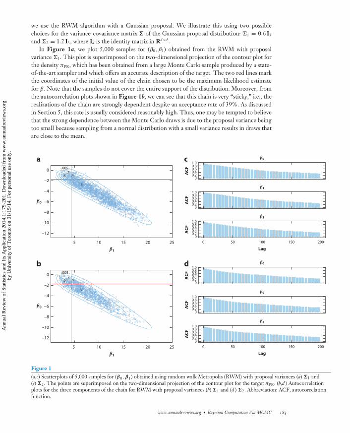
we use the RWM algorithm with a Gaussian proposal. We illustrate this using two possiblechoices for the variance-covariance matrix � of the Gaussian proposal distribution: 1 = 0.6 I3

and 2 = 1.2 I3, where Id is the identity matrix in Rd×d .In Figure 1a, we plot 5,000 samples for (β0, β1) obtained from the RWM with proposal

variance 1. This plot is superimposed on the two-dimensional projection of the contour plot forthe density πPR, which has been obtained from a large Monte Carlo sample produced by a state-of-the-art sampler and which offers an accurate description of the target. The two red lines markthe coordinates of the initial value of the chain chosen to be the maximum likelihood estimatefor β. Note that the samples do not cover the entire support of the distribution. Moreover, fromthe autocorrelation plots shown in Figure 1b, we can see that this chain is very “sticky,” i.e., therealizations of the chain are strongly dependent despite an acceptance rate of 39%. As discussedin Section 5, this rate is usually considered reasonably high. Thus, one may be tempted to believethat the strong dependence between the Monte Carlo draws is due to the proposal variance beingtoo small because sampling from a normal distribution with a small variance results in draws thatare close to the mean.

0

–2

–4

–6

–8

–10

–12

β0

β1

a.005

.2.4

.8

.6

255 10 15 20

c β0

AC

F

1.00.80.60.40.2

0

β1A

CF

1.00.80.60.40.2

0

0 50 100 150 200

Lag

β2

AC

F

1.00.80.60.40.2

0

25

0

–2

–4

–6

–8

–10

–12

5 10 15 20

β0

β1

b.005

.2.4

.8

.6

d β0

AC

F

1.00.80.60.40.2

0

β0

AC

F

1.00.80.60.40.2

0

0 50 100 150 200

Lag

β2

AC

F

1.00.80.60.40.2

0

Figure 1(a,c) Scatterplots of 5,000 samples for (β0,β1) obtained using random walk Metropolis (RWM) with proposal variances (a) �1 and(c) �2. The points are superimposed on the two-dimensional projection of the contour plot for the target πPR. (b,d ) Autocorrelationplots for the three components of the chain for RWM with proposal variances (b) �1 and (d ) �2. Abbreviation: ACF, autocorrelationfunction.


Ann

ual R

evie

w o

f St

atis

tics

and

Its

App

licat

ion

2014

.1:1

79-2

01. D

ownl

oade

d fr

om w

ww

.ann

ualr

evie

ws.

org

by U

nive

rsity

of

Tor

onto

on

01/1

5/14

. For

per

sona

l use

onl

y.


β0

5

5

10

10

–10 –8 –6 –4 –2 0 0 2 4 6 8 10 120

2

4

6

8

10

12

15

15

20

20

0

–2

–4

–6

–8

–10

β1

β2

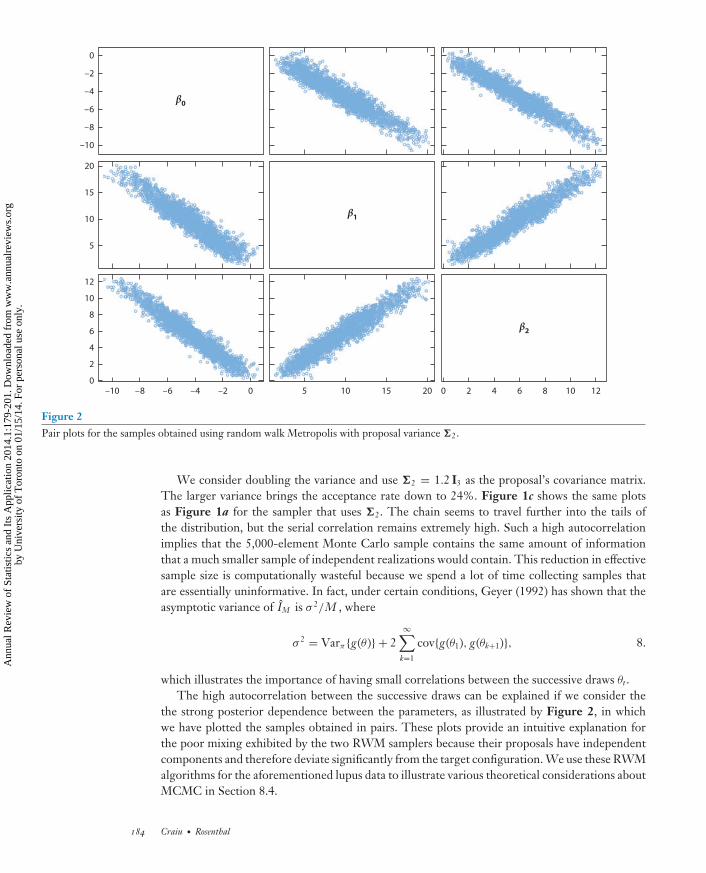
Figure 2Pair plots for the samples obtained using random walk Metropolis with proposal variance �2.

We consider doubling the variance and use �2 = 1.2 I3 as the proposal’s covariance matrix.The larger variance brings the acceptance rate down to 24%. Figure 1c shows the same plotsas Figure 1a for the sampler that uses �2. The chain seems to travel further into the tails ofthe distribution, but the serial correlation remains extremely high. Such a high autocorrelationimplies that the 5,000-element Monte Carlo sample contains the same amount of informationthat a much smaller sample of independent realizations would contain. This reduction in effectivesample size is computationally wasteful because we spend a lot of time collecting samples thatare essentially uninformative. In fact, under certain conditions, Geyer (1992) has shown that theasymptotic variance of IM is σ 2/M , where

σ 2 = Varπ {g(θ )} + 2∞∑

k=1

cov{g(θ1), g(θk+1)}, 8.

which illustrates the importance of having small correlations between the successive draws θt .The high autocorrelation between the successive draws can be explained if we consider the

the strong posterior dependence between the parameters, as illustrated by Figure 2, in whichwe have plotted the samples obtained in pairs. These plots provide an intuitive explanation forthe poor mixing exhibited by the two RWM samplers because their proposals have independentcomponents and therefore deviate significantly from the target configuration. We use these RWMalgorithms for the aforementioned lupus data to illustrate various theoretical considerations aboutMCMC in Section 8.4.


Ann

ual R

evie

w o

f St

atis

tics

and

Its

App

licat

ion

2014

.1:1

79-2

01. D

ownl

oade

d fr

om w

ww

.ann

ualr

evie

ws.

org

by U

nive

rsity

of

Tor

onto

on

01/1

5/14

. For

per

sona

l use

onl

y.


3. THE GIBBS SAMPLER

3.1. Overview of the Gibbs Sampler

The Gibbs sampler algorithm was first used by Geman & Geman (1984) in the context of imagerestoration. Subsequently, Gelfand & Smith (1992) and Tanner & Wong (1987) recognized thealgorithm’s power for fitting statistical models. Assume that the vector of parameters θ ∈ Rd ispartitioned into s subvectors so that θ = (η1, . . . , ηs ). Assume that the current state of the chain isθ (t) = (η(t)

1 , . . . , η(t)s ). The transition kernel for the Gibbs chain requires updating each subvector

in turn by sampling it from its conditional distribution, given all of the other subvectors. Moreprecisely, step t + 1 of the sampler involves the following updates:

η(t+1)1 ∼ π

(η1|η(t)

2 , . . . , η(t)s

)η

(t+1)2 ∼ π

(η2|η(t+1)

1 , η(t)3 , . . . , η(t)

s

). . . . . . . . .

η(t+1)s ∼ π

(ηs |η(t+1)

1 , η(t+1)2 , . . . , η

(t+1)s −1

).

9.

Cycling through the blocks in a fixed order defines the Gibbs sampler with deterministic scan;an alternative implementation involves a random scan in which the next block to be updated issampled at random, and each η j has a strictly positive probability of being updated. In general, it isnot known whether the Gibbs sampler with random scan is more efficient than the Gibbs samplerwith deterministic scan (Amit 1991, 1996; Liu et al. 1995). An obvious choice for the blocks η

is obtained when s = d and η j = θ j for 1 ≤ j ≤ d . Whenever possible, however, the blocks η

should contain as many individual components of θ as possible while being able to sample fromthe conditional distributions in Equation 9 (see the analysis of Liu et al. 1994).


The Gibbs sampler cannot be implemented directly because, as can be seen from Equation 6, theconditional distribution of β j given the data and all of the other parameters cannot be sampled di-rectly. However, this difficulty dissolves once we expand the model specification to include auxiliaryvariables (see also Albert & Chib 1993). Specifically, for each i ∈ {1, . . . , 55}, consider the latentvariables ψi ∼ N (xT

i β, 1), of which only the sign Yi is observed [i.e., Y i = 1(ψi > 0)]. Let X be then × p matrix with ith row xi and ψ = (ψ1, . . . , ψn). After introducing ψ , we notice that the con-ditional distributions of β|ψ, X and ψ |β, Y can be sampled directly. Alternatively, sampling fromthese two conditional distributions will yield draws from the conditional distribution p(β,ψ |X, Y ),the marginal of which, in β, is the target π (β). The Monte Carlo approach makes marginalizationeasy because we need only to drop the ψ values from the samples {(βt, ψt); 1 ≤ t ≤ M } drawnfrom p(β,ψ |X, Y ) and thereby retain only the samples {βt ; 1 ≤ t ≤ m} as draws from the targetπ (β). This computational strategy of expanding the model so that conditional distributions areavailable in closed form is known as the data augmentation (DA) algorithm (Tanner & Wong1987).

The Gibbs sampler (or DA algorithm) for the lupus data alternates between sampling from

β|ψ, X ∼ N (β, (XT X)−1),

with β = (XT X)−1XT ψ , and

ψi |β, Y i ∼ TN (xTi β, 1, Y i ),


Ann

ual R

evie

w o

f St

atis

tics

and

Its

App

licat

ion

2014

.1:1

79-2

01. D

ownl

oade

d fr

om w

ww

.ann

ualr

evie

ws.

org

by U

nive

rsity

of

Tor

onto

on

01/1

5/14

. For

per

sona

l use

onl

y.


where TN (μ, σ 2, Y ) is N (μ, σ 2) truncated to be positive if Y = 1 and negative if Y = 0. In thisformulation, η1 = (β0, β1, β2)T and η j+1 = ψ j for every j = 1, . . . , n.

The Gibbs sampling algorithm does not require tuning and does not reject any of the samplesproduced. Despite these apparent advantages, the Gibbs sampler is not always preferred overthe MH algorithm. For instance, in the PR model considered here, the chain moves slowly acrossthe parameter space. In Figure 3a we plot its trajectory for the first 300 samples when started at themaximum likelihood estimate (MLE). The sluggishness suggested by Figure 3a is confirmed bythe autocorrelation plots, which show strong and persistent serial dependence for each parameter(Figure 3b). This dependence is not necessarily a characteristic of Gibbs samplers; the highposterior dependence between parameters in the lupus data makes convergence to the target

.005

.05

.2.4.6

.8

a

β0

β1

0

–2

–4

–6

–8

–10

–12

5 10 15 20 25

b β0

AC

F

1.0

0.20.40.60.8

00 50 100 150 200

β1

AC

F

1.0

0.20.40.60.8

00 50 100 150 200

β2

Lag

AC

F

1.0

0.20.40.60.8

00 50 100 150 200

d β0

AC

F

1.0

0.20.40.60.8

00 50 100 150 200

β1

AC

F

1.0

0.20.40.60.8

00 50 100 150 200

β2

Lag

AC

F

1.0

0.20.40.60.8

00 50 100 150 200

c

β0

β1

0

–2

–4

–6

–8

–10

–12

5 10 15 20 25

.005

.05

.2.4.6

.8

Figure 3(a) Trajectory of the Gibbs chain for 300 updates for (β0, β1) (c) Scatterplots of 5,000 samples for (β0, β1) obtained usingvariable-at-a-time MH. The points are superimposed on the two-dimensional projection of the contour plot for the target πPR.(b,d ) Autocorrelation plots for the three components of the chain for (b) the Gibbs sampler and (d ) variable-at-a-time MH.Abbreviation: ACF, autocorrelation function; MH, Metropolis–Hastings.


Ann

ual R

evie

w o

f St

atis

tics

and

Its

App

licat

ion

2014

.1:1

79-2

01. D

ownl

oade

d fr

om w

ww

.ann

ualr

evie

ws.

org

by U

nive

rsity

of

Tor

onto

on

01/1

5/14

. For

per

sona

l use

onl

y.


difficult because the Gibbs sampler will always attempt to move the chain in directions that areparallel to the coordinate axes.

DA algorithms have been studied extensively owing to their intensive use in statistical mod-elling, e.g., linear and nonlinear mixed models and mixture models for which the auxiliary latentvariables are natural extensions of the model specification. Liu & Wu (1999) and Meng & vanDyk (1999) propose modified versions of the basic DA algorithm that are designed to break theserial dependence between the Monte Carlo samples and that have the potential to drasticallyimprove the mixing of the Markov chain. We refer the reader to van Dyk & Meng (2001) for animplementation of a marginal DA algorithm for the lupus data.

4. VARIABLE-AT-A-TIME METROPOLIS

4.1. Overview of Variable-at-a-Time Metropolis

Metropolis-style moves can be combined with Gibbs-style variable-at-a-time moves to create avariable-at-a-time Metropolis algorithm. [This algorithm is also sometimes called Metropolis-within-Gibbs, but it was actually the original form of the algorithm used by Metropolis et al.(1953).]

Assume again that the vector of parameters θ ∈ Rd is partitioned into s subvectors such thatθ = (η1, . . . , ηs ). Variable-at-a-time Metropolis then proceeds by proposing to move just onecoordinate (or subset of coordinates) at a time, leaving all other coordinates fixed. In its mostcommon form, we might try to move the ith coordinate by proposing a new state ωt+1, whereωt+1, j = ηt, j for all j = i , and where ηt,i ∼ N (ηt,i , σ

2). (Here ωt+1, j is the jth coordinate of ωt+1,etc.) We then accept the proposal ωt+1 according to the MH rule (see Equation 7).

As with the Gibbs sampler, we need to choose which coordinate to update each time.Again, we can proceed either by choosing coordinates in the sequence 1, 2, . . . , d , 1, 2, . . .

(systematic-scan) or by choosing the coordinate to update uniformly from {1, 2, . . . , d } on eachiteration (random-scan). (In this formulation, one systematic-scan iteration is roughly equivalentto d random-scan ones.)

The variable-at-a-time Metropolis algorithm is often a good generic choice. Unlike the fullMetropolis algorithm, it does not require moving all coordinates at once (which can be challengingto do efficiently). In addition, unlike Gibbs sampling, variable-at-a-time Metropolis does notrequire the ability to sample from the full conditional distributions (which could be infeasible).


We now try using a componentwise RWM to update each coordinate of β. Specifically, theproposal ωt+1,h is generated from N (βt,h, σ

2h ) at time t + 1 for each coordinate h and is accepted

with probabilitymin{1, π (ωt+1,h |βt,[−h])/π (βt,h |βt,[−h])}, 10.

where βt,[−h] is the vector of the most recent updates for all the components of β except βh . Notethat the ratio involved in Equation 10 is identical to π (ωt+1,h, βt,[−h])/π (βt,h, βt,[−h]) and can becomputed in closed form because it is independent of any unknown normalizing constants.

We have implemented the algorithm using σ = (√

5, 5, 2√

2). These values were chosen toyield acceptance rates for each component of between 20% and 25%. Figure 3c shows the samplesobtained, and Figure 3d presents the autocorrelation functions. Notice that although the serialdependence is smaller than in the full MH implementation, it remains high. Also, the samplescover most of the support of the posterior density π . In the one-at-a-time implementation, we are


Ann

ual R

evie

w o

f St

atis

tics

and

Its

App

licat

ion

2014

.1:1

79-2

01. D

ownl

oade

d fr

om w

ww

.ann

ualr

evie

ws.

org

by U

nive

rsity

of

Tor

onto

on

01/1

5/14

. For

per

sona

l use

onl

y.


no longer forcing all components of the chain to move together simultaneously, which seems toimprove the spread of the resulting sample.

5. OPTIMIZING AND ADAPTING THE RANDOM WALKMETROPOLIS ALGORITHM

Consider the RWM algorithm with proposals ωt = θt + εt , where εt ∼ N (0, ) (i.i.d.). Althoughvery specific, this algorithm still allows for great flexibility in the choice of proposal covariancematrix . This raises the question of what leads to the best performance of the algorithm, whichwe now discuss.

5.1. Optimal Scaling

We first note that if the elements on the diagonal of are very small, then the proposals ωt willusually be very close to the previous states θt . Thus, the proposals will usually be accepted, but thechain will hardly move, which is clearly suboptimal. However, if is very large, then the proposalsωt will usually be very far from the previous states θt . Thus, these proposals (especially in highdimensions) will likely be out in the tails of the target density π in at least one coordinate andthus will likely have much lower π values. This implies that they will almost always be rejected,which is again clearly suboptimal. The optimal scaling, then, is somewhere in between these twoextremes. That is, we want our proposal scaling to be neither too small nor too large. Rather, itshould be “just right” (this is sometimes called the Goldilocks principle).

In a pioneering paper, Roberts and colleagues (1997) took this a step further, proving that (fora certain idealized high-dimensional limit, at least) the optimal acceptance rate (i.e., the limitingfraction of accepted proposed moves) is equal to the specific fraction 0.234, ∼23%. However, anyacceptance rate between ∼15% and 50% is still fairly efficient (see, e.g., Roberts & Rosenthal2001, figure 3). Later optimal scaling results obtained by Roberts & Rosenthal (2001) and Bedard(2006) indicate that (again, for a certain idealized high-dimensional limit) the optimal proposalcovariance should be chosen to be proportional to the true covariance matrix of the targetdistribution π (with the constant of proportionality chosen to achieve the 0.234 acceptance rate).In Figure 4, we compare two RWM chains with similar acceptance rates but different choices of

−15 −10 −5 0 5 10 15

0

1,000

2,000

3,000

4,000

5,000

x

Ite

rati

on

nu

mb

er

a

0

1,000

2,000

3,000

4,000

5,000

x

Ite

rati

on

nu

mb

er

−15 −10 −5 0 5 10 15

b

Figure 4Trace plots of the first coordinate of random walk Metropolis on the same 20-dimensional target. Acceptance rates in both plots areapproximately 0.234, and the proposal covariance matrix is proportional to either (a) the identity I20 or (b) the target covariancematrix. The run in (b) clearly mixes much faster.


Ann

ual R

evie

w o

f St

atis

tics

and

Its

App

licat

ion

2014

.1:1

79-2

01. D

ownl

oade

d fr

om w

ww

.ann

ualr

evie

ws.

org

by U

nive

rsity

of

Tor

onto

on

01/1

5/14

. For

per

sona

l use

onl

y.


the proposal distribution variance. The chain for which the variance of the proposal distributionis proportional to that of the target exhibits considerably better mixing.

5.2. Adaptive Markov Chain Monte Carlo

Unfortunately, one generally has little idea about the true covariance of π at the beginning of asimulation. Thus, direct application of the optimal scaling results of the previous section is difficultor impossible. One possible approach is to first perform a number of exploratory MCMC runsto get an idea of the geography of the target’s important regions and to then use this knowledgeto tune the proposal to be approximately optimal. However, this approach requires restarting thechain multiple times, using each run to tune different subsets of the simulation parameters. Becausethis process can be lengthy and onerous, especially in high-dimensional spaces, it generally haslimited success in complex models.

Alternatively, one can build upon the recent advances in adaptive MCMC (AMCMC) in whichthe proposal distribution is updated continuously at any time t using the information containedin the samples obtained up until that time (see, e.g., Bai et al. 2011, Craiu et al. 2009, Haarioet al. 2001, Roberts & Rosenthal 2009). Such an approach does not require restarting the chainand can be fully automated. However, this approach requires careful theoretical analysis becausethe process loses its Markovian property by using the past realizations of the chain (instead ofusing only its current state), and asymptotic ergodicity must be proven on a case-by-case basis.Fortunately, the general frameworks developed by, e.g., Andrieu et al. (2005) and Roberts &Rosenthal (2007), have made proving the validity of adaptive samplers easier.


We have implemented the adaptive RWM proposed by Haario et al. (2001) (see also Roberts &Rosenthal 2009) in which at each time t > 1,000, we use the following approximation for in theGaussian proposal:

t = (2.4)2

3SamVart + εI3, 11.

where ε = 0.01 and SamVart is the sample variance of all samples drawn up to time t − 1. Thisadaptation attempts to mimic the theoretical optimal scaling results discussed in Section 5.1; ifSamVart happened to equal the true covariance matrix of π and if ε = 0, then Equation 11 wouldindeed be the optimal proposal covariance. Figure 5 shows the same plots as those generatedfor Figure 1a–d. The reduction in serial autocorrelation is apparent. For instance, the mean,median, lower quartile, and upper quartile for the autocorrelations of the RWM sampler with 2

computed up to lag 200 equal 0.537, 0.513, 0.377, and 0.664, respectively; they equal the muchsmaller values 0.065, 0.029, 0.007, and 0.059, respectively, for the adaptive RWM.

6. SIMULATED TEMPERING

Particular challenges arise in MCMC when the target density π is multimodal, i.e., the targetdensity has distinct high-probability regions separated by low-probability barriers that are difficultfor the Markov chain to traverse. In such cases, a simple MCMC algorithm such as RWM mayeasily explore well within any one modal region, but the chain may take an unfeasibly long timeto move between modes. This leads to extremely slow convergence and poor resulting estimates.

Simulated tempering attempts to flatten out the distribution into related distributions with lesspronounced modes that can be sampled more easily. If done carefully, simulated tempering can


Ann

ual R

evie

w o

f St

atis

tics

and

Its

App

licat

ion

2014

.1:1

79-2

01. D

ownl

oade

d fr

om w

ww

.ann

ualr

evie

ws.

org

by U

nive

rsity

of

Tor

onto

on

01/1

5/14

. For

per

sona

l use

onl

y.


β0

AC

F

0.4

0.8

00 50 100 150 200

β0

AC

F

0.4

0.8

00 50 100 150 200

β0

AC

F

0.4

0.8

00 50 100 150 200

Lagβ1

β0

0

–2

–4

–6

–8

–10

–12

5 10 15 20 25

.005

.05

.2.4.6.8

Figure 5Left panel: Scatterplot of 30,000 samples for (β0,β1) obtained using random walk Metropolis (RWM) with adaptive variance. Thepoints are superimposed on the two-dimensional projection of the contour plot for the target πPR. Right panels: Autocorrelation plotsfor the three components of the chain show much lower serial dependence when compared with nonadaptive RWM samplers.Abbreviation: ACF, autocorrelation function.

compensate for this flattening out, ultimately yielding good estimates for expected values fromthe original target density π , as explained below.

Specifically, simulated tempering requires a sequence π1, π2, . . . , πm of target densities, whereπ1 = π is the original density and πτ is flatter for the distributions for which τ is large. (Theparameter τ is usually referred to as the temperature, making π1 the cold density and πτ for largervalues of τ the so-called hot densities.) These different densities can then be combined to definea single joint density π on � × {1, 2, . . . , m}, defined by π (θ, τ ) = 1

m πτ (θ ) for 1 ≤ τ ≤ m andθ ∈ �. (Weights other than the uniform choice, 1

m , may also be used.)Simulated tempering then uses π to define a joint Markov chain (θ, τ ) on � × {1, 2, . . . , m},

with target density π . In the simplest case, this chain is a version of variable-at-a-time Metropolisthat alternates (say) between spatial moves, which propose (say) θ ′ ∼ N (θ, σ 2

θ ) and accept withthe usual Metropolis probability min(1,

π (θ ′,�τ )π (θ,�τ ) ) = min(1,

πτ (θ ′)πτ (θ ) ), and temperature moves, which

propose (say) τ ′ = τ ± 1 (with a probability of 12 each) and accept with the usual Metropolis

probability min(1,π (θ,τ ′)π (θ,τ ) ) = min(1,

πτ ′ (θ )πτ (θ ) ).

As is usual for Metropolis algorithms, this chain should converge in distribution to the densityπ . But, of course, our interest is in the original density π = π1, not in π . The genius of simulatedtempering is that ultimately, we count only those samples corresponding to τ = 1. That is, oncewe have a good sample from π , we simply discard all the sample values corresponding to τ = 1,and what remains is a good sample from π .

6.1. A Simple Example

For a specific example, suppose the target density is given by π (θ ) = 12 N (0, 1; θ ) + 1

2 N (20, 1; θ ).This target density is a mixture of the standard normal density N (0, 1; θ ) and the normal densityN (20, 1; θ ) with mean 20 and variance 1. This chain is highly multimodal (Figure 6a), leading tovery poor mixing of ordinary RWM (Figure 7a).

However, if πτ (θ ) = 12 N (0, τ 2; θ ) + 1

2 N (20, τ 2; θ ), i.e., a mixture of two normal densitieswith means 0 and 20 but with variances τ 2 instead of 1, then π1 = π is the original target


Ann

ual R

evie

w o

f St

atis

tics

and

Its

App

licat

ion

2014

.1:1

79-2

01. D

ownl

oade

d fr

om w

ww

.ann

ualr

evie

ws.

org

by U

nive

rsity

of

Tor

onto

on

01/1

5/14

. For

per

sona

l use

onl

y.


a

0

0.05

0.10

0.15

0.20tf

(x)

–10 0 10 20 30x

b0.05

0.04

0.03

0.02

0.01

–10 0 10 20 30x

c

0.022

0.020

0.018

0.016

0.014

0.012

0.024

–10 0 10 20 30x

Figure 6(a) The highly multimodal target density π (θ ) = 1

2 N (0, 1; θ ) + 12 N (20, 1; θ ). (b) A somewhat flatter density

π4 = 12 N (0, 42; θ ) + 1

2 N (20, 42; θ ). (c) An even flatter density π10 = 12 N (0, 102; θ ) + 1

2 N (20, 102; θ ).

density, but πτ becomes flatter for larger τ (Figure 6a–c). This behavior allows us to define ajoint simulated tempering chain on π (with proposal scaling σθ = 1, say), which mixes much fasterowing to the flattened high-temperature distributions (Figure 7b). We can then identify the θ

values corresponding to τ = 1 in this faster-mixing joint chain to get a very good sample fromπ1 = π (Figure 7c). As with all Monte Carlo sampling, a good sample from π allows us to computegood estimates for expected values I = E(g) for functionals g of interest.

a40

20

–20

0 10,000 20,000 30,000 40,000 50,000

0

Index

xli

st

xli

st

b40

20

–20

0 10,000 20,000 30,000 40,000 50,000

0

Index

c40

20

–20

0 10,000 20,000 30,000 40,000 50,000

0

Index

xli

st (

, 1)

d20

15

10

5

0

10,0008,0006,0004,0002,0000

Index

xli

st

Figure 7Trace plots for the highly multimodal target density π (θ ) = 1

2 N (0, 1; θ ) + 12 N (20, 1; θ ). (a) Ordinary random walk Metropolis gets

stuck in the modal region of π near 20 and cannot find the second modal region near 0. (b) The θ coordinates of simulated temperingfor π . (c) Red circles indicate the θ values of the simulated tempering corresponding to τ = 1 (and hence to π ). (d ) The θ1 coordinatesfor the corresponding parallel tempering algorithm, showing excellent mixing.


Ann

ual R

evie

w o

f St

atis

tics

and

Its

App

licat

ion

2014

.1:1

79-2

01. D

ownl

oade

d fr

om w

ww

.ann

ualr

evie

ws.

org

by U

nive

rsity

of

Tor

onto

on

01/1

5/14

. For

per

sona

l use

onl

y.


6.2. Choosing the Tempered Distributions

Simulated tempering often works quite well, but it raises the question of how to find appropriatetempered distributions πτ . Usually, we will not know convenient choices such as the one givenabove, πτ = 1

2 N (0, τ 2) + 12 N (20, τ 2). Thus, we require more generic choices.

One promising approach is to let the hotter densities πτ (θ ) correspond to taking smaller andsmaller powers of the original target density π (θ ), i.e., to let πτ (θ ) = c τ (π (θ ))1/τ for an appropriatenormalizing constant c τ . (It is common to write β = 1/τ and refer to β as the inverse temperature.)This formula guarantees that π1 = π and that πτ will be flatter for larger τ (because small positivepowers move all positive numbers closer to 1), which is precisely what we need. As a specificexample, if π (θ ) happened to be the density of N (μ, σ 2), then c τ (π (θ ))1/τ would be the density ofN (μ, τσ 2). This is indeed a flatter density, similar to the simple example above, which confirmsthat this approach holds promise.

Unfortunately, this approach has the following problem. If we propose to move τ to τ ′, thenwith this formula, we should accept this proposal with probability

min(

1,πτ ′ (θ )πτ (θ )

)= min

(1,

c τ ′

c τ

(π (θ ))(1/τ ′)−(1/τ ))

.

This formula explicitly depends on the normalizing constants c τ and c τ ′ ; these constants do notcancel as they do in ordinary RWM. This dependence is problematic because the values of c τ areusually unknown and infeasible to calculate. So, what can be done?

6.3. Parallel Tempering

One idea is to use parallel tempering, sometimes called Metropolis-coupled MCMC (MCMCMC).In this algorithm, the state space is �m, corresponding to m different chains, each with its ownvalue of θ . So, the state at time t is given by θt = (θt1, θt2, . . . , θtm). Intuitively, each θtτ is at its owntemperature τ , i.e., converging towards its own target density πτ . The overall target density isnow π (θ ) = π1(θ1)π2(θ2) . . . πm(θm), i.e., the density that makes each coordinate of θ independentand following the density of its own temperature. For any 1 ≤ τ ≤ m, then, the algorithm canupdate the chain θt−1,τ at temperature τ by proposing (say) θ ′

t,τ ∼ N (θt−1,τ , σ2) and accepting this

proposal with the usual Metropolis probability min(1,πτ (θ ′

t,τ )πτ (θt−1,τ ) ).

Crucially, the chain can also choose temperatures τ and τ ′ (perhaps choosing each temperatureuniformly from {1, 2, . . . , m}), and it can then propose to swap the values θn,τ and θt,τ ′ . Thisproposal will then be accepted with its usual Metropolis probability, min(1,

πτ (θt,τ ′ )πτ ′ (θt,τ )πτ (θt,τ )πτ ′ (θt,τ ′ ) ). The

beauty of parallel tempering is that it allows the normalizing constants to cancel. That is, ifπτ (θ ) = c τ (π (θ ))1/τ , then the acceptance probability becomes

min

(1,

c τ π (θt,τ ′ )1/τ c τ ′π (θt,τ )1/τ ′

c τ π (θt,τ )1/τ c τ ′π (θt,τ ′ )1/τ ′

)= min

(1,

π (θt,τ ′ )1/τπ (θt,τ )1/τ ′

π (θt,τ )1/τπ (θt,τ ′ )1/τ ′

).

Thus, the values of c τ and c τ ′ are not required to run the algorithm.As a first test, we can apply parallel tempering to the simple example given above, again using

πτ (θ ) = 12 N (0, τ 2; θ )+ 1

2 N (20, τ 2; θ ) for τ = 1, 2, . . . , 10. Parallel tempering works pretty well inthis case (Figure 7d ). Of course, the normalizing constants in this example were known, so paralleltempering was not really required. However, these constants are unknown in many applications;parallel tempering is often a useful sampling method in such cases.


Ann

ual R

evie

w o

f St

atis

tics

and

Its

App

licat

ion

2014

.1:1

79-2

01. D

ownl

oade

d fr

om w

ww

.ann

ualr

evie

ws.

org

by U

nive

rsity

of

Tor

onto

on

01/1

5/14

. For

per

sona

l use

onl

y.


7. ASSESSING MARKOV CHAIN MONTE CARLO ERRORS

When considering any statistical estimation procedure, the amount of uncertainty in the estimate,e.g., some measure of its standard error, is an important issue. In conventional Monte Carloalgorithms, where the {θi } are i.i.d., as in Equation 3, the standard error is given by 1√

MSD(g(θ )),

where SD(g(θ )) is the usual estimate of the standard deviation of the distribution of the g(θi ).However, with MCMC there is usually extensive serial correlation in the samples θi , so the usuali.i.d.-based estimate of standard error does not apply. So-called perfect sampling algorithms arean exception [see, for example, Propp & Wilson (1996) or Craiu & Meng (2011)], but they arehard to adapt for Bayesian computation. Indeed, the standard error for MCMC is usually bothlarger than in the i.i.d. case (owing to the correlations) and harder to quantify.

The simplest way to estimate standard error from an MCMC estimate is to rerun the entireMarkov chain several times using the same values of run length M and burn-in B as in Equation 4but starting from different initial values θ0 drawn from the same overdispersed (i.e., well spread-out)initial distribution. This process leads to a sequence of i.i.d. estimates of the target expectationI, and standard errors from the resulting sequence of estimates can then be computed in theusual i.i.d. manner. (We illustrate this in Section 8.4 using the RWM algorithms for the lupusdata presented in Section 2.1.) However, such a procedure is often highly inefficient, raising thequestion of how to estimate standard error from a single run of a single Markov chain. Specifically,we would like to estimate v ≡ Var( 1

M −B

∑Mi=B+1 g(θi )).

7.1. Variance Estimate

To estimate the variance of v above, let g(θ ) = g(θ ) − E(g), so E(g) = 0. And, assume that B islarge enough that θi ≈ π for i > B. Then, writing ≈ to mean “equal in the limit as M → ∞,”we compute that

v ≈ E

⎡⎣((

1M − B

M∑i=B+1

g(θi )

)− E(g)

)2⎤⎦ = E

⎡⎣(

1M − B

M∑i=B+1

g(θi )

)2⎤⎦

= 1(M − B)2

[(M − B)E(g(θi )2) + 2(M − B − 1)E(g(θi )g(θi+1))

+ 2(M − B − 2)E(g(θi )g(θi+2)) + · · ·]≈ 1

M − B(E(g(θi )2) + 2E(g(θi )g(θi+1)) + 2E(g(θi )g(θi+2)) + · · ·)

= 1M − B

(Varπ (g) + 2Covπ (g(θi )g(θi+1)) + 2Covπ (g(θi )g(θi+2)) + · · ·)

= 1M − B

Varπ (g) (1 + 2Corrπ (g(θi ), g(θi+1)) + 2Corrπ (g(θi ), g(θi+2)) + · · ·)

≡ 1M − B

Varπ (g)(ACT ) = (i.i.d . variance) (ACT ),

where i.i.d. variance is the value for the variance that we would obtain if the samples {θ i} were infact i.i.d., and

ACT = 1 + 2∞∑

k=1

Corrπ (g(θ0), g(θk)) ≡ 1 + 2∞∑

k=1

ρk =∞∑

k=−∞ρk = 2

( ∞∑k=0

ρk

)− 1

is the factor by which the variance is multiplied owing to the serial correlations from the Markovchain (sometimes called the integrated autocorrelation time). Here, Corrπ refers to the theoreticalcorrelation that would arise from a sequence {θi }∞

i=−∞ that was in stationarity (so each θ i had densityπ ) and that followed the Markov chain transitions. This assumption implies that the correlations


Ann

ual R

evie

w o

f St

atis

tics

and

Its

App

licat

ion

2014

.1:1

79-2

01. D

ownl

oade

d fr

om w

ww

.ann

ualr

evie

ws.

org

by U

nive

rsity

of

Tor

onto

on

01/1

5/14

. For

per

sona

l use

onl

y.


are a function of the time lag between the two variables and, in particular, that ρ−k = ρk as above.The standard error is then given by s e = √

v = (i.i.d . − s e)√

ACT .Now, both the i.i.d. variance and the quantity ACT can be estimated from the sample run. (For

example, the built-in ACF function in R automatically computes the lag correlations ρk. Note alsothat when computing ACT in practice, we do not sum over all k. Rather, we sum only until, say,|ρk| < 0.05 or ρk < 0, because for large k we should have ρk ≈ 0 but the estimates of ρk will alwayscontain some sampling error.) This procedure provides a method of estimating the standard errorof the sample. It also provides a method of comparing different MCMC algorithms because inmost cases, ACT � 1 and better chains would have smaller ACT values. In the most extremecase, one sometimes even tries to design antithetic chains for which ACT < 1 (see Adler 1981,Barone & Frigessi 1990, Craiu & Lemieux 2007, Craiu & Meng 2005, Neal 1995).

7.2. Confidence Intervals

Suppose we estimate u ≡ E(g) by the quantity e = 1M −B

∑Mi=B+1 g(θi ) and obtain an estimate e

and an approximate variance (as above) v. Then what is, say, a 95% confidence interval for u?Well, if a central limit theorem (CLT) applies (as discussed in Section 8), then for large values

of M − B, we have the normal approximation that e ≈ N (u, v). It then follows as usual that(e − u)v−1/2 ≈ N (0, 1), so P(−1.96 < (e − u)v−1/2 < 1.96) ≈ 0.95, so P(−1.96

√v < e − u <

1.96√

v) ≈ 0.95. This gives us our desired confidence interval: With a probability of 95%, theinterval (e −1.96

√v, e +1.96

√v) will contain u. (Strictly speaking, we should use the t distribution,

not the normal distribution. But if M − B is at all large, then the t and normal distributions arevery similar. Thus, we can ignore this issue for now.) Such confidence intervals allow us to moreappropriately assess the uncertainty of our MCMC estimates (e.g., Flegal et al. 2008).

The above analysis raises the question of whether a CLT even holds for Markov chains. Weanswer this and other questions when we consider the theory of MCMC in the following section.

8. THEORETICAL FOUNDATIONS OF MARKOV CHAINMONTE CARLO

We close with some theoretical considerations about MCMC. Specifically, why does MCMCwork? The key is that the distribution of θn converges in various senses to the target distributionπ (·). This convergence follows from basic Markov chain theory, as we discuss below.

8.1. Markov Chain Convergence

A basic fact about Markov chains is that if a Markov chain is irreducible and aperiodic, withstationarity distribution π , then θt converges in distribution to π as t → ∞. More precisely, wehave Theorem 1 (see, e.g., Meyn & Tweedie 1993, Roberts & Rosenthal 2004, Rosenthal 2001,Tierney 1994).

Theorem 1: If a Markov chain is irreducible, with stationarity probability density π ,then for π-a.e. initial value θ0: (a) if g :� → R with E(|g|) < ∞, then lim

n→∞1n

∑ni=1 g(θi ) =

E(g) ≡ ∫g(θ )π (θ )dθ , and (b) if the chain is also aperiodic, then furthermore lim

t→∞P(θt ∈

S) = ∫S π (θ ) dθ for all measurable S ⊆ �.

We now discuss the various conditions of the theorem, one at a time.


Ann

ual R

evie

w o

f St

atis

tics

and

Its

App

licat

ion

2014

.1:1

79-2

01. D

ownl

oade

d fr

om w

ww

.ann

ualr

evie

ws.

org

by U

nive

rsity

of

Tor

onto

on

01/1

5/14

. For

per

sona

l use

onl

y.


Being irreducible means, essentially, that the chain has positive probability of eventually gettingfrom any one location to any other. In the discrete case, we can define irreducibility as sayingthat for all i, j ∈ � there exists t ∈ N such that P(θt = j |θ0 = i ) > 0. In the general case,however, this definition is problematic because the probability of hitting any particular state isusually zero. Instead, we can define irreducibility (or φ-irreducibility) as saying that there is somereference measure φ such that for all ζ ∈ �, and for all A ⊆ � with φ(A) > 0, there existst ∈ N such that P(θt ∈ A|θ0 = ζ ) > 0. This condition is usually satisfied for MCMC (aside fromcertain rare cases in which the state space consists of highly disjoint pieces) and is generally not aconcern.

Being aperiodic means that there are no forced cycles, i.e., that there do not exist disjointnonempty subsets �1,�2, . . . , �d ⊆ � for some d ≥ 2 such that P (θt+1 ∈ �i+1|θt = ζ ) = 1for all ζ ∈ �i (1 ≤ i ≤ d − 1), and P (θt+1 ∈ �1|θt = ζ ) = 1 for all ζ ∈ �d . This conditionvirtually always holds for MCMC. For example, it holds (a) if P (θt+1 = ζ |θt = ζ ) > 0, as forthe Metropolis algorithm (owing to the positive probability of rejection); (b) if two iterations aresometimes equivalent to just one, as for the Gibbs sampler; or (c) if the transition probabilities havepositive densities throughout �, as is often the case. In short, we have never known aperiodicityto be a problem for MCMC.

The condition that the density π be stationary for the chain is the most subtle one, as we discussnext.

8.2. Reversibility and Stationarity of Markov Chains

For ease of notation, this section focuses on discrete Markov chains, although the general case issimilar upon replacing probability mass functions with measures and sums with integrals. We thuslet π be a probability mass function on � and assume for simplicity that π (θ ) > 0 for all θ ∈ �.We also let P (i, j ) = P(θ1 = j |θ0 = i ) be the Markov chain’s transition probabilities.

We say that π is stationary for the Markov chain if it is preserved under the chain’s dynamics,i.e., if the chain has the property that whenever θ0 ∼ π [meaning that P(θ0 = i ) = π (i ) for alli ∈ �], then also θ1 ∼ π [i.e., P(θ1 = i ) = π (i ) for all i ∈ �]. Equivalently,

∑i∈� π (i )P (i, j ) = π ( j )

for all j ∈ �. Intuitively, this means that the probabilities π are left invariant by the chain, whichexplains why the chain might converge to those probabilities in the limit.

We now show that reversibility is automatically satisfied by MH algorithms, thereby explainingwhy the Metropolis acceptance probabilities are defined as they are. Indeed, let q (i, j ) = P(ωt =j |θt−1 = i ) be the proposal distribution, which is then accepted with probability min(1,

π ( j )q ( j,i )π (i )q (i, j ) ).

Then, for i, j ∈ � with i = j ,

P (i, j ) = q (i, j ) min(

1,π ( j )q ( j, i )π (i )q (i, j )

).

It follows that

π (i )P (i, j ) = π (i )q (i, j ) min(

1,π ( j )q ( j, i )π (i )q (i, j )

)= min(π (i )q (i, j ), π ( j )q ( j, i )).

By inspection, this last expression is symmetric in i and j. It then follows that π (i )P (i, j ) =π ( j )P ( j, i ) for all i, j ∈ � (at least for i = j , but the case i = j is trivial). This property isdescribed as π being reversible for the chain. [Intuitively, reversibility implies that if θ0 ∼ π ,then P(θ0 = i, θ1 = j ) = P(θ0 = j, θ1 = i ), i.e., the probability of starting at i and movingto j is the same as that of starting at j and moving to i. This property is also called being timereversible.]


Ann

ual R

evie

w o

f St

atis

tics

and

Its

App

licat

ion

2014

.1:1

79-2

01. D

ownl

oade

d fr

om w

ww

.ann

ualr

evie

ws.

org

by U

nive

rsity

of

Tor

onto

on

01/1

5/14

. For

per

sona

l use

onl

y.


The importance of reversibility is that it implies stationarity of π . Indeed, using reversibility,we compute that if θ0 ∼ π , then

P(θ1 = j ) =∑i∈�

P(θ0 = i )P(i, j ) =∑i∈�

π (i )P (i, j ) =∑i∈�

π ( j )P ( j, i )

= π ( j )∑i∈�

P ( j, i ) = π ( j ).

Thus, θ1 ∼ π , too, so π is stationary.We conclude that the stationarity condition holds automatically for any MH algorithm. Hence,

assuming irreducibility and aperiodicity (which, as noted above, are virtually always satisfied forMCMC), Theorem 1 applies and establishes the asymptotic validity of MCMC.

8.3. Markov Chain Monte Carlo Convergence Rates

Write Pt(ζ, S) = P[θt ∈ S|θ0 = ζ ] for the t-step transition probabilities for the chain, and letD(ζ, t) = ||Pt(ζ, ·) − �(·)|| supS⊆� |Pt(ζ, S) − �(S)| be a measure (specifically, the total variationdistance) of the chain’s distance from stationarity after t steps, where �(S) = ∫

S π (ζ ) dζ is thetarget probability distribution. Then, the chain is said to be ergodic if limt→∞ D(ζ, t) = 0 for π-a.e. ζ ∈ �, i.e., if the chain transition probabilities Pt(ζ, S) converge (uniformly) to � as t → ∞,which Theorem 1 indicates is usually true for MCMC. However, ergodicity alone says nothingabout the convergence rate, i.e., how quickly this convergence occurs.

By contrast, a quantitative bound on convergence is an actual number t∗ such that D(ζ, t∗) <

0.01, i.e., such that the chain’s probabilities are within 0.01 of stationary after t∗ iterations. (Thecutoff value 0.01 is arbitrary but has become fairly standard.) We then sometimes say that the chain“converges in t∗ iterations.” Quantitative bounds, when available, are the most useful because theyprovide precise instructions about how long an MCMC algorithm must be run. Unfortunately,these bounds are often difficult to establish for complicated statistical models, although someprogress has been made (e.g., Douc et al. 2004; Jones & Hobert 2001; Rosenthal 1995, 2002).

Halfway between these two extremes is geometric ergodicity, which is more useful than plainergodicity but which is often easier to compute than are quantitative bounds. A chain is geomet-rically ergodic if there are ρ < 1 and �-a.e.-finite M :� → [0, ∞] such that D(ζ, t) ≤ M (ζ )ρt

for all ζ ∈ � and t ∈ N, i.e., such that the convergence to � happens exponentially quickly.If a Markov chain is geometrically ergodic and g :� → R such that E(|g|2+a ) < ∞ for some

a > 0, then a CLT holds for quantities such as e = 1M −B

∑Mi=B+1 g(θi ) (Geyer 1992, Tierney

1994), and we have the normal approximation that e ≈ N (u, v). [In fact, if the Markov chain isreversible as above, then it suffices to take a = 0 (Roberts & Rosenthal 1997).] As explained inSection 7.2, this approximation is key to obtaining confidence intervals and thus more reliableestimates.

Now, if the state space � is finite, then assuming irreducibility and aperiodicity, any Markovchain on � is always geometrically ergodic. However, this result is not true for infinite statespaces. The RWM algorithm is known to be geometrically ergodic essentially (i.e., under a fewmild technical conditions) if and only if π has exponential tails, i.e., there are a, b, c > 0 such thatπ (θ ) ≤ ae−b |θ | whenever |θ | > c (Mengersen & Tweedie 1996, Roberts & Tweedie 1996). TheGibbs sampler is known to be geometrically ergodic for certain models (e.g., Papaspiliopoulos &Roberts 2008). But in some cases, geometric ergodicity can be difficult to ascertain.

In the absence of theoretical convergence bounds, it is difficult to determine whether the chainhas reached stationarity. One option is to independently run some large number K of chains,each with an initial state drawn from the same overdispersed starting distribution. If M and Bare large enough, we expect the estimators provided by each chain to approximately agree. For


Ann

ual R

evie

w o

f St

atis

tics

and

Its

App

licat

ion

2014

.1:1

79-2

01. D

ownl

oade

d fr

om w

ww

.ann

ualr

evie

ws.

org

by U

nive

rsity

of

Tor

onto

on

01/1

5/14

. For

per

sona

l use

onl

y.


mathematical formalization of this general principle see, e.g., Gelman & Rubin (1992) and Brooks& Gelman (1998).

8.4. Convergence of Random Walk Metropolis for the Lupus Data

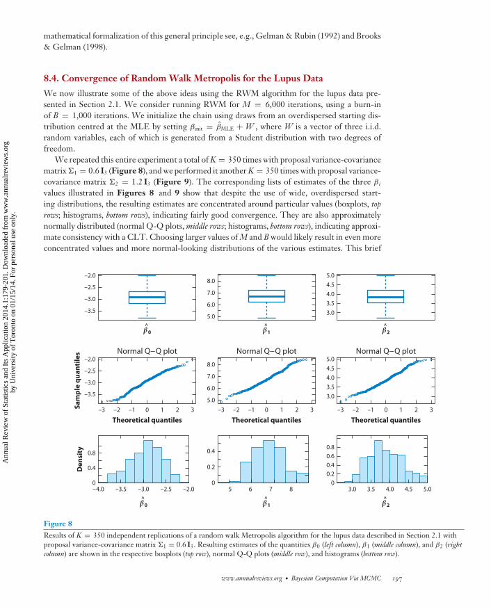
We now illustrate some of the above ideas using the RWM algorithm for the lupus data pre-sented in Section 2.1. We consider running RWM for M = 6,000 iterations, using a burn-inof B = 1,000 iterations. We initialize the chain using draws from an overdispersed starting dis-tribution centred at the MLE by setting βinit = βMLE + W , where W is a vector of three i.i.d.random variables, each of which is generated from a Student distribution with two degrees offreedom.

We repeated this entire experiment a total of K = 350 times with proposal variance-covariancematrix 1 = 0.6 I3 (Figure 8), and we performed it another K = 350 times with proposal variance-covariance matrix 2 = 1.2 I3 (Figure 9). The corresponding lists of estimates of the three β i

values illustrated in Figures 8 and 9 show that despite the use of wide, overdispersed start-ing distributions, the resulting estimates are concentrated around particular values (boxplots, toprows; histograms, bottom rows), indicating fairly good convergence. They are also approximatelynormally distributed (normal Q-Q plots, middle rows; histograms, bottom rows), indicating approxi-mate consistency with a CLT. Choosing larger values of M and B would likely result in even moreconcentrated values and more normal-looking distributions of the various estimates. This brief

–2.0

–2.5

–3.0

–3.5

β^

0

Normal Q−Q plot

Theoretical quantiles

Sa

mp

le q

ua

nti

les

–2.0

–2.5

–3.0

–3.5

–3 –2 –1 1 2 30

De

nsi

ty

β^

0

0

0.4

0.8

–4.0 –3.5 –3.0 –2.5 –2.0

5.0

6.0

7.0

8.0

β^

1

Normal Q−Q plot

5.0

6.0

7.0

8.0


–3 –2 –1 1 2 30

β^

1

0

0.2

0.4

5 6 7 8

β^

2

3.03.54.04.55.0

Normal Q−Q plot


–3 –2 –1 1 2 30

3.03.54.04.55.0

β^

2

0.80.60.40.2

03.0 3.5 4.0 4.5 5.0

Figure 8Results of K = 350 independent replications of a random walk Metropolis algorithm for the lupus data described in Section 2.1 withproposal variance-covariance matrix 1 = 0.6 I3. Resulting estimates of the quantities β0 (left column), β1 (middle column), and β2 (rightcolumn) are shown in the respective boxplots (top row), normal Q-Q plots (middle row), and histograms (bottom row).


Ann

ual R

evie

w o

f St

atis

tics

and

Its

App

licat

ion

2014

.1:1

79-2

01. D

ownl

oade

d fr

om w

ww

.ann

ualr

evie

ws.

org

by U

nive

rsity

of

Tor

onto

on

01/1

5/14

. For

per

sona

l use

onl

y.


–2.0

–2.5

–3.0

–3.5

β^

0

Normal Q−Q plot


Sa

mp

le q

ua

nti

les

–2.0

–2.5

–3.0

–3.5

–3 –2 –1 1 2 30

De

nsi

ty

β^

0

0

0.4

0.8

–4.0 –3.5 –3.0 –2.5 –2.0

5.0

6.0

7.0

8.0

β^

1

Normal Q−Q plot

5.0

6.0

7.0

8.0


–3 –2 –1 1 2 30

β^

1

0

0.2

0.4

5 6 7 8

β^

2

3.03.54.04.55.0

Normal Q−Q plot


–3 –2 –1 1 2 30

3.03.54.04.55.0

β^

2

0.80.60.40.2

03.0 3.5 4.0 4.5 5.0

Figure 9Results of K = 350 independent replications of a random walk Metropolis algorithm for the lupus data described in Section 2.1 withproposal variance-covariance matrix 2 = 1.2 I3. Resulting estimates of the quantities β0 (left column), β1 (middle column), and β2 (rightcolumn) are shown in the resulting boxplots (top row), normal Q-Q plots (middle row), and histograms (bottom row).

experiment illustrates that even in the absence of theoretical convergence bounds, one can usemultiple independent runs from overdispersed starting distributions to assess the convergence,accuracy, and normality of MCMC estimates.

8.5. The Case of the Independence Sampler

When it comes to MCMC convergence rates, one case is particularly tractable, namely the inde-pendence sampler. Unsurprisingly, as long as an independence sampler’s proposal satisfies q (θ ) > 0whenever π (θ ) > 0, irreducibility, aperiodicity, and stationarity all follow easily, and Theorem 1therefore immediately establishes ergodicity. What is remarkable, however, is that the indepen-dence sampler is geometrically ergodic if and only if there is δ > 0 such that q (θ ) ≥ δπ (θ ) forπ-a.e. θ ∈ �, and furthermore in this case D(ζ, n) ≤ (1 − δ)n for π-a.e. ζ ∈ � (Mengersen &Tweedie 1996, Roberts & Tweedie 1996). That is, for the independence sampler, we have notonly an easy test for geometric ergodicity but also a free quantitative bound.

For a simple, specific example, consider an independence sampler on � = [0, ∞) with targetdensity π (θ ) = e−θ . If the proposal density is, say, q (θ ) = 0.01 e−0.01θ , then q (θ ) ≥ 0.01 π (θ )for all θ ∈ �. That is, the above condition for ergodicity holds when δ = 0.01: The chain isgeometrically ergodic with D(ζ, t) ≤ (1− δ)t = (0.99)t and hence converges in t∗ = 459 iterations[because (0.99)459 < 0.01]. By contrast, if q (θ ) = 5e−5θ , then the above condition does not holdfor any value δ > 0. Thus, the chain is not geometrically ergodic. In fact, Rosenthal & Roberts(2011) showed that in this case 4,000,000 ≤ t∗ ≤ 14,000,000, i.e., the chain takes at least four


Ann

ual R

evie

w o

f St

atis

tics

and

Its

App

licat

ion

2014

.1:1

79-2

01. D

ownl

oade

d fr

om w

ww

.ann

ualr

evie

ws.

org

by U

nive

rsity

of

Tor

onto

on

01/1

5/14

. For

per

sona

l use

onl

y.


million iterations to converge. This example illustrates how geometric ergodicity can sometimesmake a tremendous difference between MCMC algorithms that converge efficiently and those thatconverge very poorly. Moreover, it illustrates once again how MCMC methodology can help usexplore target probability distributions and understand their statistical properties. The interplaybetween practical implementation and theoretical analysis involves many novel ideas with greatpotential for future development.

DISCLOSURE STATEMENT

The authors are not aware of any affiliations, memberships, funding, or financial holdings thatmight be perceived as affecting the objectivity of this review.

ACKNOWLEDGMENTS

We thank Nancy Reid for encouraging us to write this review, and we thank the anonymousreferee for a very careful reading that led to many improvements.

LITERATURE CITED

Adler SL. 1981. Over-relaxation methods for the Monte Carlo evaluation of the partition function for multi-quadratic actions. Phys. Rev. D 23:2901–4

Albert JH, Chib S. 1993. Bayesian analysis of binary and polychotomous response data. J. Am. Stat. Assoc.88:669–79

Amit Y. 1991. On rates of convergence of stochastic relaxation for Gaussian and non-Gaussian distributions.J. Multivar. Anal. 38:82–100

Amit Y. 1996. Convergence properties of the Gibbs sampler for perturbations of Gaussians. Ann. Stat. 24:122–40

Andrieu C, Moulines E, Priouret P. 2005. Stability of stochastic approximation under verifiable conditions.SIAM J. Control Optim. 44:283–312

Bai Y, Craiu RV, DiNarzo AF. 2011. Divide and conquer: a mixture-based approach to regional adaptationfor MCMC. J. Comput. Graph. Stat. 20:63–79

Barone P, Frigessi A. 1990. Improving stochastic relaxation for Gaussian random fields. Probab. Eng. Inf. Sci.4:369–89

Bedard M. 2006. On the robustness of optimal scaling for random walk Metropolis algorithms. PhD Thesis, Depart-ment of Statistics, Univ. Toronto

Brooks S, Gelman A, Jones GL, Meng X-L, eds. 2011. Handbook of Markov Chain Monte Carlo. Boca Raton,FL: Chapman & Hall/CRC

Brooks SP, Gelman A. 1998. General methods for monitoring convergence of iterative simulations. J. Comput.Graph. Stat. 7:434–55

Casarin R, Craiu RV, Leisen F. 2013. Interacting multiple try algorithms with different proposal distributions.Stat. Comput. 23:185–200

Chen M-H, Shao Q-M, Ibrahim JG. 2000. Monte Carlo Methods in Bayesian Computation. New York: SpringerCraiu RV, Lemieux C. 2007. Acceleration of the multiple-try Metropolis algorithm using antithetic and

stratified sampling. Stat. Comput. 17:109–20Craiu RV, Meng X-L. 2005. Multi-process parallel antithetic coupling for forward and backward MCMC.

Ann. Stat. 33:661–97Craiu RV, Meng X-L. 2011. Perfection within reach: exact MCMC sampling. In Handbook of Markov Chain

Monte Carlo, ed. S Brooks, A Gelman, GL Jones, X-L Meng, pp. 199–226. Boca Raton, FL: Chapman &Hall/CRC

Craiu RV, Rosenthal JS, Yang C. 2009. Learn from thy neighbor: parallel-chain adaptive and regional MCMC.J. Am. Stat. Assoc. 104:1454–66


Ann

ual R

evie

w o

f St

atis

tics

and

Its

App

licat

ion

2014

.1:1

79-2

01. D

ownl

oade

d fr

om w

ww

.ann

ualr

evie

ws.

org

by U

nive

rsity

of

Tor

onto

on

01/1

5/14

. For

per

sona

l use

onl

y.


Douc R, Moulines E, Rosenthal JS. 2004. Quantitative bounds on convergence of time-inhomogeneousMarkov chains. Ann. Appl. Probab. 14:1643–65

Flegal JM, Haran M, Jones GL. 2008. Markov chain Monte Carlo: Can we trust the third significant figure?Stat. Sci. 23:250–60

Gelfand AE, Smith AFM. 1990. Sampling-based approaches to calculating marginal densities. J. Am. Stat.Assoc. 85:398–409

Gelman A, Rubin DB. 1992. Inference from iterative simulation using multiple sequences. Stat. Sci. 7:457–72Geman S, Geman D. 1984. Stochastic relaxation, Gibbs distributions, and the Bayesian restoration of images.

IEEE Trans. Pattern Anal. Mach. Intell. 6:721–41Geyer CJ. 1992. Practical Markov chain Monte Carlo (with discussion). Stat. Sci. 7:473–83Green PJ. 1995. Reversible jump Markov chain Monte Carlo computation and Bayesian model determination.

Biometrika 82:711–32Green PJ, Mira A. 2001. Delayed rejection in reversible jump Metropolis-Hastings. Biometrika 88:1035–53Haario H, Saksman E, Tamminen J. 2001. An adaptive Metropolis algorithm. Bernoulli 7:223–42Hastings WK. 1970. Monte Carlo sampling methods using Markov chains and their applications. Biometrika

57:97–109Jones G, Hobert J. 2001. Honest exploration of intractable probability distributions via Markov chain Monte

Carlo. Stat. Sci. 16:312–34Liu JS. 2001. Monte Carlo Strategies in Scientific Computing. New York: SpringerLiu JS, Liang F, Wong WH. 2000. The multiple-try method and local optimization in Metropolis sampling.

J. Am. Stat. Assoc. 95:121–34Liu JS, Wong WH, Kong A. 1994. Covariance structure of the Gibbs sampler with applications to the

comparisons of estimators and augmentation schemes. Biometrika 81:27–40Liu JS, Wong WH, Kong A. 1995. Covariance structure and convergence rate of the Gibbs sampler with

various scans. J. R. Stat. Soc. B 57:157–69Liu JS, Wu YN. 1999. Parameter expansion for data augmentation. J. Am. Stat. Assoc. 94:1264–74Meng X-L, van Dyk DA. 1999. Seeking efficient data augmentation schemes via conditional and marginal

augmentation. Biometrika 86:301–20Mengersen KL, Tweedie RL. 1996. Rates of convergence of the Hastings and Metropolis algorithms. Ann.

Stat. 24:101–21Metropolis N, Rosenbluth AW, Rosenbluth MN, Teller AH, Teller E. 1953. Equations of state calculations

by fast computing machines. J. Chem. Phys. 21:1087–92Meyn SP, Tweedie RL. 1993. Markov Chains and Stochastic Stability. London: Springer-VerlagNeal RM. 1995. Suppressing random walks in Markov chain Monte Carlo using ordered overrelaxation. Tech.

Rep. 9508, Univ. Toronto. Dep. Stat., Toronto, Can. http://arxiv.org/pdf/bayes-an/9506004v1.pdfPapaspiliopoulos O, Roberts GO. 2008. Stability of the Gibbs sampler for Bayesian hierarchical models. Ann.

Stat. 36:95–117Propp JG, Wilson DB. 1996. Exact sampling with coupled Markov chains and applications to statistical

mechanics. Random Struct. Algorithms 9:223–52Richardson S, Green PJ. 1997. On Bayesian analysis of mixtures with an unknown number of components

(with discussion). J. R. Stat. Soc. B 59:731–92Robert CP, Casella G. 2004. Monte Carlo Statistical Methods. New York: SpringerRobert CP, Casella G. 2010. Introducing Monte Carlo Methods with R. New York: SpringerRoberts GO, Gelman A, Gilks WR. 1997. Weak convergence and optimal scaling of random walk Metropolis

algorithms. Ann. Appl. Probab. 7:110–20Roberts GO, Rosenthal JS. 1997. Geometric ergodicity and hybrid Markov chains. Electron. Commun. Probab.

2(2):13–25Roberts GO, Rosenthal JS. 2001. Optimal scaling for various Metropolis-Hastings algorithms. Stat. Sci.

16:351–67Roberts GO, Rosenthal JS. 2004. General state space Markov chains and MCMC algorithms. Probab. Surv.

1:20–71Roberts GO, Rosenthal JS. 2007. Coupling and ergodicity of adaptive Markov chain Monte Carlo algorithms.

J. Appl. Probab. 44:458–75


Ann

ual R

evie

w o

f St

atis

tics

and

Its

App

licat

ion

2014

.1:1

79-2

01. D

ownl

oade

d fr

om w

ww

.ann

ualr

evie

ws.

org

by U

nive

rsity

of

Tor

onto

on

01/1

5/14

. For

per

sona

l use

onl

y.

http://arxiv.org/pdf/bayes-an/9506004v1.pdf


Roberts GO, Rosenthal JS. 2009. Examples of adaptive MCMC. J. Comput. Graph. Stat. 18:349–67Roberts GO, Tweedie RL. 1996. Geometric convergence and central limit theorems for multidimensional

Hastings and Metropolis algorithms. Biometrika 83:95–110Rosenthal JS. 1995. Minorization conditions and convergence rates for Markov chain Monte Carlo. J. Am.

Stat. Assoc. 90:558–66Rosenthal JS. 2001. A review of asymptotic convergence for general state space Markov chains. Far East J.

Theor. Stat. 5:37–50Rosenthal JS. 2002. Quantitative convergence rates of Markov chains: a simple account. Electron. Commun.

Probab. 7:123–28Rosenthal JS, Roberts GO. 2011. Quantitative non-geometric convergence bounds for independence samplers.

Methodol. Comput. Appl. Probab. 13:391–403Spiegelhalter DJ, Best NG, Carlin BP, Van Der Linde A. 2002. Bayesian measures of model complexity and

fit (with discussion). J. R. Stat. Soc. B 64:583–639Tanner MA, Wong WH. 1987. The calculation of posterior distributions by data augmentation. J. Am. Stat.

Assoc. 82:528–40Tierney L. 1994. Markov chains for exploring posterior distributions. Ann. Stat. 22:1701–28van Dyk DA, Meng X-L. 2001. The art of data augmentation (with discussion). J. Comput. Graph. Stat.

10:1–111


Ann

ual R

evie

w o

f St

atis

tics

and

Its

App

licat

ion

2014

.1:1

79-2

01. D

ownl

oade

d fr

om w

ww

.ann

ualr

evie

ws.

org

by U

nive

rsity

of

Tor

onto

on

01/1

5/14

. For

per

sona

l use

onl

y.

ST01-FrontMatter ARI 25 November 2013 21:12

Annual Review ofStatistics and ItsApplication

Volume 1, 2014ContentsWhat Is Statistics?

Stephen E. Fienberg � � � � � � � � � � � � � � � � � � � � � � � � � � � � � � � � � � � � � � � � � � � � � � � � � � � � � � � � � � � � � � � � � � � � � � � � � � � 1

A Systematic Statistical Approach to Evaluating Evidence fromObservational StudiesDavid Madigan, Paul E. Stang, Jesse A. Berlin, Martijn Schuemie,

J. Marc Overhage, Marc A. Suchard, Bill Dumouchel, Abraham G. Hartzema,and Patrick B. Ryan � � � � � � � � � � � � � � � � � � � � � � � � � � � � � � � � � � � � � � � � � � � � � � � � � � � � � � � � � � � � � � � � � � � � � � � �11

The Role of Statistics in the Discovery of a Higgs BosonDavid A. van Dyk � � � � � � � � � � � � � � � � � � � � � � � � � � � � � � � � � � � � � � � � � � � � � � � � � � � � � � � � � � � � � � � � � � � � � � � � � � � �41

Brain Imaging AnalysisF. DuBois Bowman � � � � � � � � � � � � � � � � � � � � � � � � � � � � � � � � � � � � � � � � � � � � � � � � � � � � � � � � � � � � � � � � � � � � � � � � � � �61

Statistics and ClimatePeter Guttorp � � � � � � � � � � � � � � � � � � � � � � � � � � � � � � � � � � � � � � � � � � � � � � � � � � � � � � � � � � � � � � � � � � � � � � � � � � � � � � � � �87

Climate Simulators and Climate ProjectionsJonathan Rougier and Michael Goldstein � � � � � � � � � � � � � � � � � � � � � � � � � � � � � � � � � � � � � � � � � � � � � � � � � 103

Probabilistic ForecastingTilmann Gneiting and Matthias Katzfuss � � � � � � � � � � � � � � � � � � � � � � � � � � � � � � � � � � � � � � � � � � � � � � � � 125

Bayesian Computational ToolsChristian P. Robert � � � � � � � � � � � � � � � � � � � � � � � � � � � � � � � � � � � � � � � � � � � � � � � � � � � � � � � � � � � � � � � � � � � � � � � � � 153

Bayesian Computation Via Markov Chain Monte CarloRadu V. Craiu and Jeffrey S. Rosenthal � � � � � � � � � � � � � � � � � � � � � � � � � � � � � � � � � � � � � � � � � � � � � � � � � � � 179

Build, Compute, Critique, Repeat: Data Analysis with LatentVariable ModelsDavid M. Blei � � � � � � � � � � � � � � � � � � � � � � � � � � � � � � � � � � � � � � � � � � � � � � � � � � � � � � � � � � � � � � � � � � � � � � � � � � � � � � � 203

Structured Regularizers for High-Dimensional Problems: Statistical andComputational IssuesMartin J. Wainwright � � � � � � � � � � � � � � � � � � � � � � � � � � � � � � � � � � � � � � � � � � � � � � � � � � � � � � � � � � � � � � � � � � � � � 233

High-Dimensional Statistics with a View Toward Applications in BiologyPeter Buhlmann, Markus Kalisch, and Lukas Meier � � � � � � � � � � � � � � � � � � � � � � � � � � � � � � � � � � � � � 255

v

Ann

ual R

evie

w o

f St

atis

tics

and

Its

App

licat

ion

2014

.1:1

79-2

01. D

ownl

oade

d fr

om w

ww

.ann

ualr

evie

ws.

org

by U

nive

rsity

of

Tor

onto

on

01/1

5/14

. For

per

sona

l use

onl

y.

ST01-FrontMatter ARI 25 November 2013 21:12

Next-Generation Statistical Genetics: Modeling, Penalization, andOptimization in High-Dimensional DataKenneth Lange, Jeanette C. Papp, Janet S. Sinsheimer, and Eric M. Sobel � � � � � � � � � � � � � 279

Breaking Bad: Two Decades of Life-Course Data Analysis inCriminology, Developmental Psychology, and BeyondElena A. Erosheva, Ross L. Matsueda, and Donatello Telesca � � � � � � � � � � � � � � � � � � � � � � � � � � � � 301

Event History AnalysisNiels Keiding � � � � � � � � � � � � � � � � � � � � � � � � � � � � � � � � � � � � � � � � � � � � � � � � � � � � � � � � � � � � � � � � � � � � � � � � � � � � � � � � 333

Statistical Evaluation of Forensic DNA Profile EvidenceChristopher D. Steele and David J. Balding � � � � � � � � � � � � � � � � � � � � � � � � � � � � � � � � � � � � � � � � � � � � � � 361

Using League Table Rankings in Public Policy Formation:Statistical IssuesHarvey Goldstein � � � � � � � � � � � � � � � � � � � � � � � � � � � � � � � � � � � � � � � � � � � � � � � � � � � � � � � � � � � � � � � � � � � � � � � � � � � 385

Statistical EcologyRuth King � � � � � � � � � � � � � � � � � � � � � � � � � � � � � � � � � � � � � � � � � � � � � � � � � � � � � � � � � � � � � � � � � � � � � � � � � � � � � � � � � � � 401

Estimating the Number of Species in Microbial Diversity StudiesJohn Bunge, Amy Willis, and Fiona Walsh � � � � � � � � � � � � � � � � � � � � � � � � � � � � � � � � � � � � � � � � � � � � � � � 427

Dynamic Treatment RegimesBibhas Chakraborty and Susan A. Murphy � � � � � � � � � � � � � � � � � � � � � � � � � � � � � � � � � � � � � � � � � � � � � � � 447

Statistics and Related Topics in Single-Molecule BiophysicsHong Qian and S.C. Kou � � � � � � � � � � � � � � � � � � � � � � � � � � � � � � � � � � � � � � � � � � � � � � � � � � � � � � � � � � � � � � � � � � 465

Statistics and Quantitative Risk Management for Banking and InsurancePaul Embrechts and Marius Hofert � � � � � � � � � � � � � � � � � � � � � � � � � � � � � � � � � � � � � � � � � � � � � � � � � � � � � � � 493

vi Contents

Ann

ual R

evie

w o

f St

atis

tics

and

Its

App

licat

ion

2014

.1:1

79-2

01. D

ownl

oade

d fr

om w

ww

.ann

ualr

evie

ws.

org

by U

nive

rsity

of

Tor

onto

on

01/1

5/14

. For

per

sona

l use

onl

y.

bayesian computation via markov chain monte...

Documents