Baum-Welch and HMM applications

December 4, 2018

Markov chains

3 states of weather: sunny, cloudy, rainyObserved once a day at the same time

All transitions are possible, with some probabilityEach state depends only on the previous state

Hidden Markov Models

All we observe is the dog:

IOOOIPIIIOOOOOPPIIIIIPIWhat’s the underlying weather (the hidden states)?

How likely is this sequence, given our model of how the dog works?

What portion of the sequence was generated by each state?

Hidden Markov Models: the three questions

EvaluationGiven a HMM, M, and a sequence of observations, xFind P(x|M)

DecodingGiven a HMM, M, and a sequence of observations, xFind the sequence Q of hidden states that maximizes P(x, Q|M)

LearningGiven an unknown HMM, M, and a sequence of observations, xFind parameters θ that maximize P(x|θ, M)

review

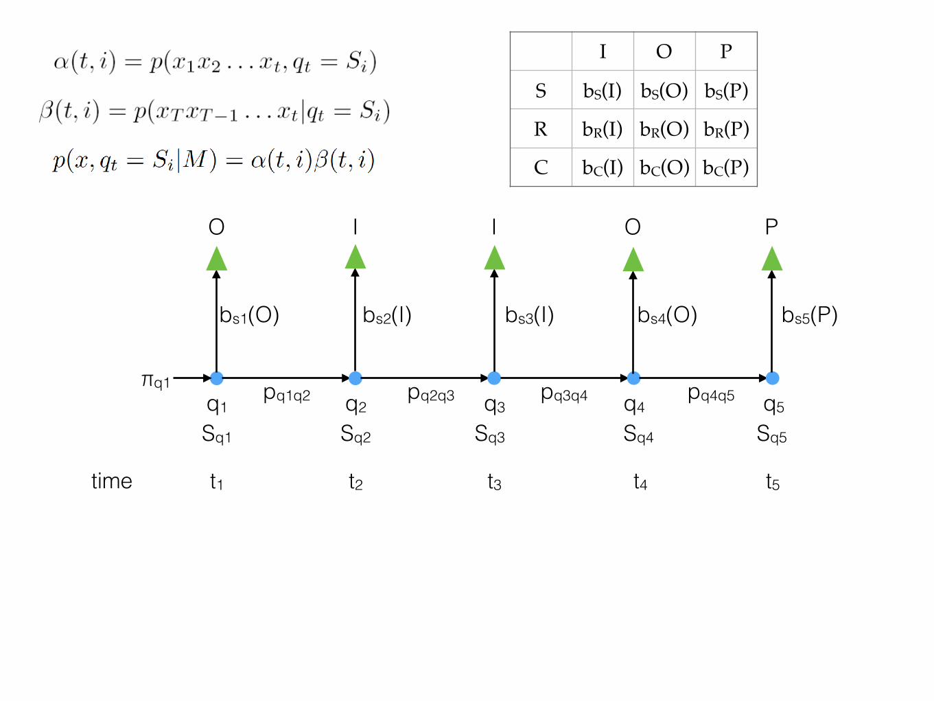
x are observations ∈ A, q1...qn are hidden states ∈ S

time t1 t2 t3 t4 t5

q1 q2 q3 q4 q5

x1 x2 x3 x4 x5

Sq1 Sq2 Sq3 Sq4 Sq5

bs1(x1) bs2(x2) bs3(x3) bs4(x4) bs5(x5)

pq1q2 pq2q3 pq3q4 pq4q5πq1

Baum-Welch expectation maximization algorithm

You have: observed data

You want: parameters of the HMM that generated that data

Problem: the calculation space is too big for exact calculation -> use heuristic method (even though it’s a partial solution it’s very useful!)

We are finding locally optimal parameters.

Baum-Welch expectation maximization algorithm

Assume: data come from some random process that we can fit to a HMM

Assumption #1: alphabet A and the number of states, N, are fixed. Transition, emission and initial distribution probabilities are all unknown.

Baum-Welch expectation maximization algorithm

Assumption #2: data are a set of observed sequences {x(d)} each of which has a hidden state sequence Qd

Assumption #3: we can set all parameters/probabilities to some initial values Can choose from some uniform distributionCan choose to incorporate some prior knowledgeCan just be randomCannot be flat

Baum-Welch expectation maximization algorithm

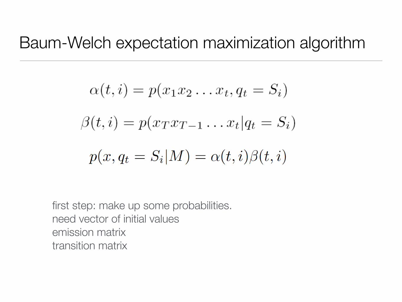
first step: make up some probabilities. need vector of initial values emission matrix transition matrix

Baum-Welch expectation maximization algorithm

x1x2x3...xtxt+1...xT-1xT

q1q2q3...qtqt+1...qT-1qT

...SiSl...

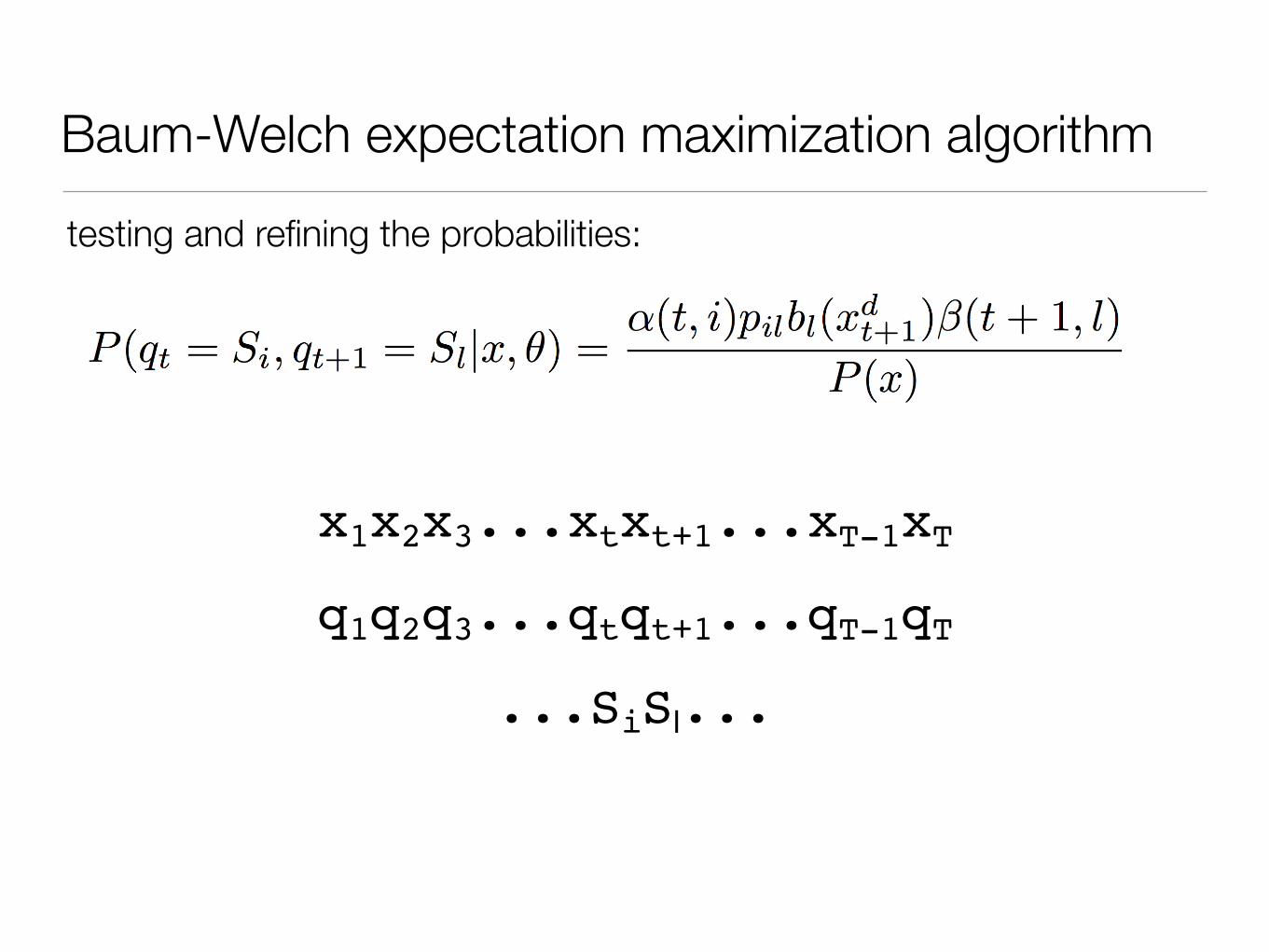
testing and refining the probabilities:

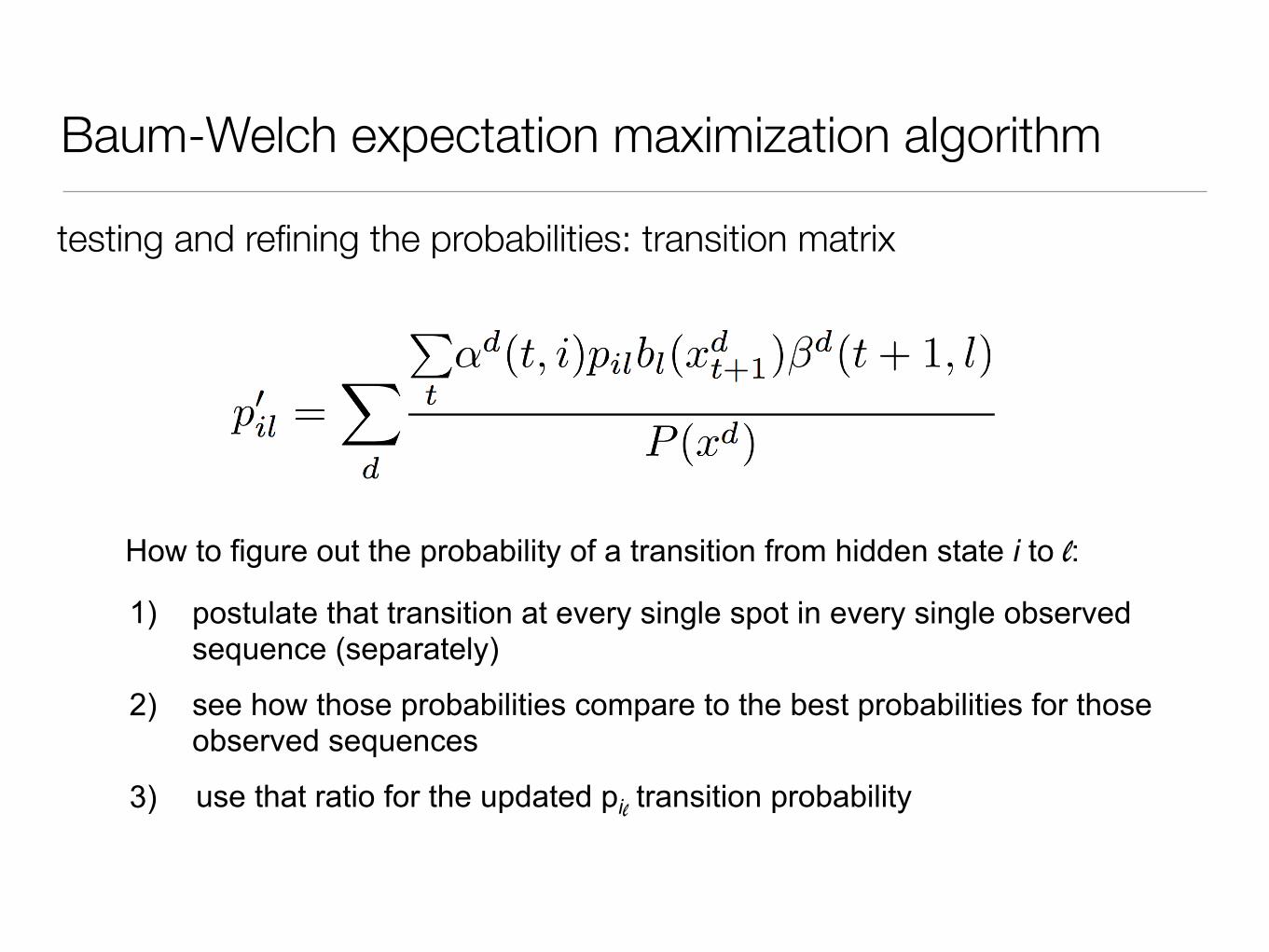
How to figure out the probability of a transition from hidden state i to l:

1) postulate that transition at every single spot in every single observed sequence (separately)

2) see how those probabilities compare to the best probabilities for those observed sequences

3) use that ratio for the updated pil transition probability

Baum-Welch expectation maximization algorithm

testing and refining the probabilities: transition matrix

Figure out the probability of an emission of symbol a from hidden state l 1) postulate that hidden state under every symbol a in every single

observed sequence (separately)

2) see how those probabilities compare to the best probabilities for those observed sequences

3) use that ratio for the updated b’l(a) transition probability

Baum-Welch expectation maximization algorithm

testing and refining the probabilities: emission matrix

Baum-Welch expectation maximization algorithm

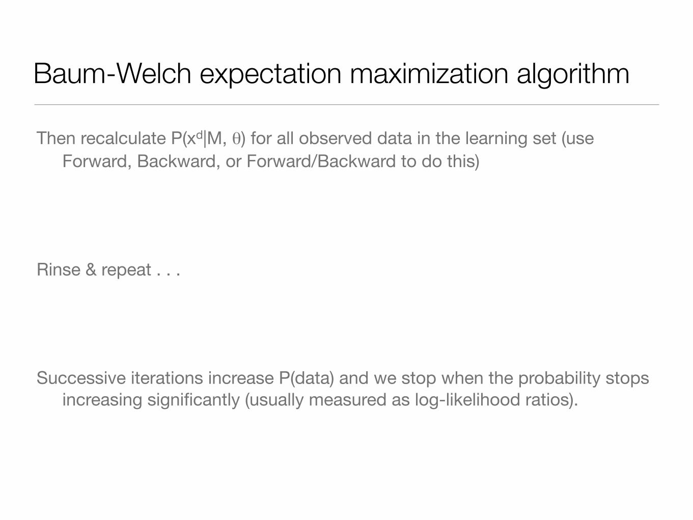
Then recalculate P(xd|M, θ) for all observed data in the learning set (use Forward, Backward, or Forward/Backward to do this)

Rinse & repeat . . .

Successive iterations increase P(data) and we stop when the probability stops increasing significantly (usually measured as log-likelihood ratios).

Baum-Welch example

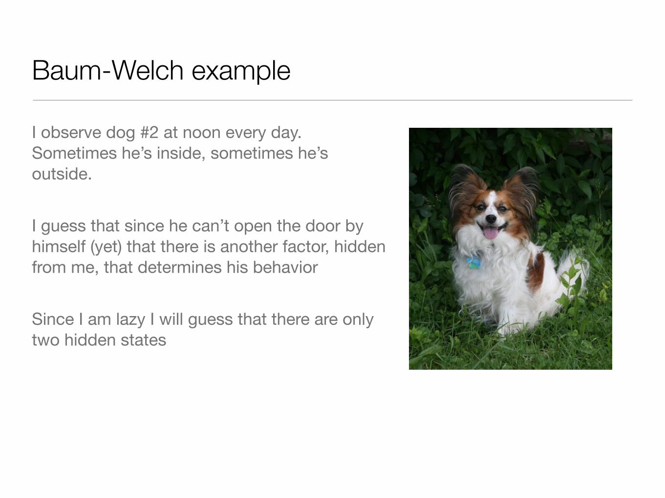
I observe dog #2 at noon every day. Sometimes he’s inside, sometimes he’s outside.

I guess that since he can’t open the door by himself (yet) that there is another factor, hidden from me, that determines his behavior

Since I am lazy I will guess that there are only two hidden states

Baum-Welch example

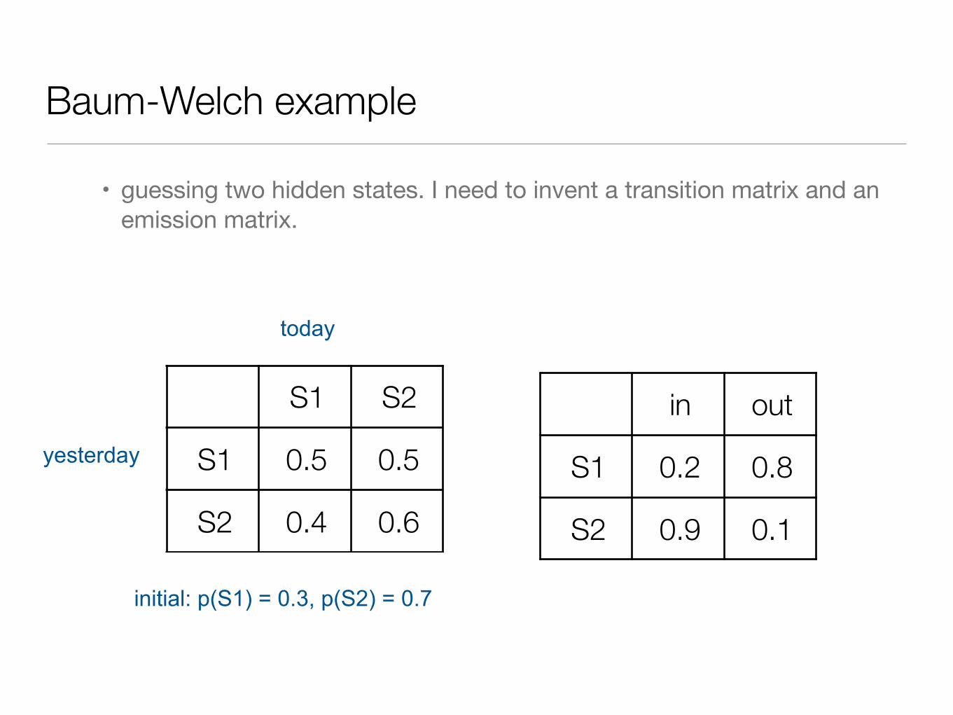
• guessing two hidden states. I need to invent a transition matrix and an emission matrix.

S1 S2

S1 0.5 0.5

S2 0.4 0.6

yesterday

today

in out

S1 0.2 0.8

S2 0.9 0.1

initial: p(S1) = 0.3, p(S2) = 0.7

Baum-Welch example

one set of observations: II, II, II, II, IO, OO, OI, II, II

S1 S2

S1 0.5 0.5

S2 0.4 0.6

yesterday

today

in out

S1 0.2 0.8

S2 0.9 0.1

initial: p(S1) = 0.3, p(S2) = 0.7

Baum-Welch example

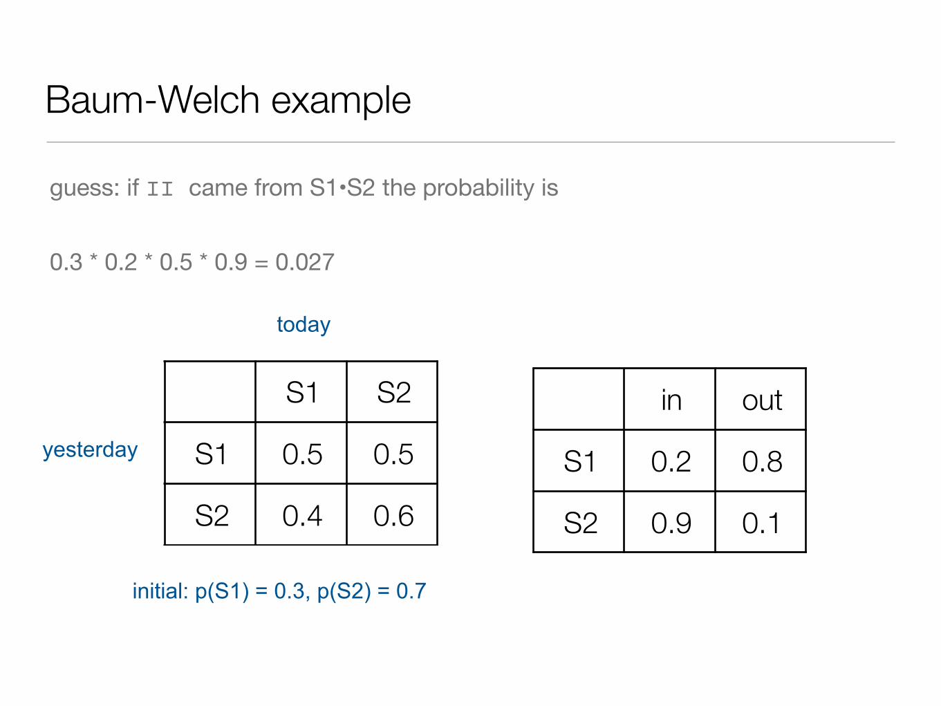
guess: if II came from S1•S2 the probability is

0.3 * 0.2 * 0.5 * 0.9 = 0.027

S1 S2

S1 0.5 0.5

S2 0.4 0.6

yesterday

today

in out

S1 0.2 0.8

S2 0.9 0.1

initial: p(S1) = 0.3, p(S2) = 0.7

Baum-Welch example

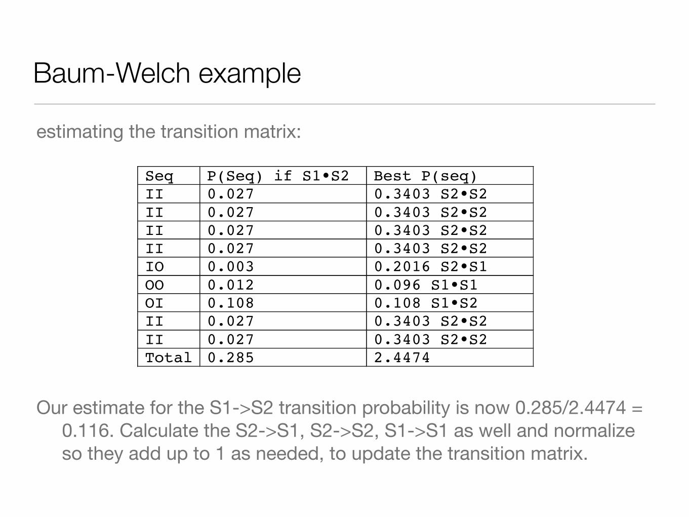
estimating the transition matrix:

Our estimate for the S1->S2 transition probability is now 0.285/2.4474 = 0.116. Calculate the S2->S1, S2->S2, S1->S1 as well and normalize so they add up to 1 as needed, to update the transition matrix.

Seq P(Seq) if S1•S2 Best P(seq) II 0.027 0.3403 S2•S2 II 0.027 0.3403 S2•S2 II 0.027 0.3403 S2•S2 II 0.027 0.3403 S2•S2 IO 0.003 0.2016 S2•S1 OO 0.012 0.096 S1•S1 OI 0.108 0.108 S1•S2 II 0.027 0.3403 S2•S2 II 0.027 0.3403 S2•S2 Total 0.285 2.4474

Baum-Welch example

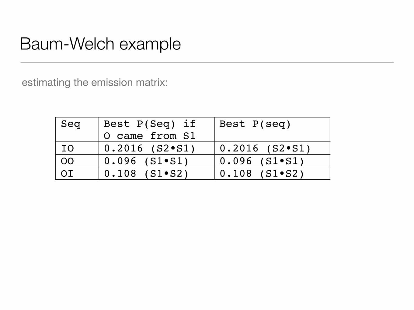
estimating the emission matrix:

Seq Best P(Seq) if O came from S1

Best P(seq)

IO 0.2016 (S2•S1) 0.2016 (S2•S1) OO 0.096 (S1•S1) 0.096 (S1•S1) OI 0.108 (S1•S2) 0.108 (S1•S2)

Baum-Welch example

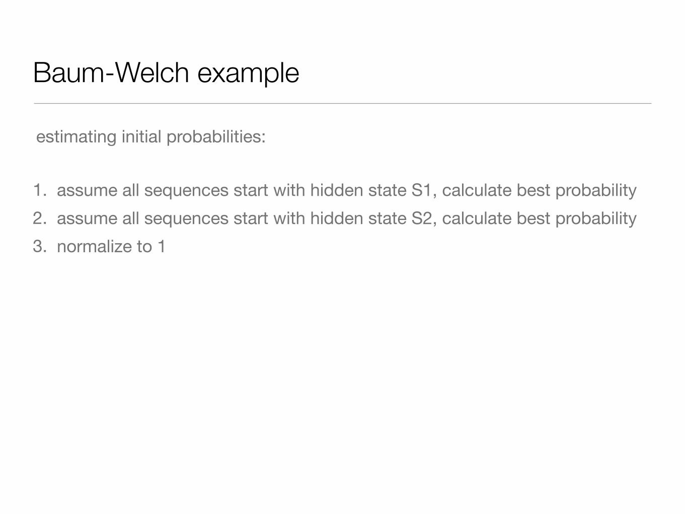
estimating initial probabilities:

1. assume all sequences start with hidden state S1, calculate best probability2. assume all sequences start with hidden state S2, calculate best probability3. normalize to 1

Baum-Welch example

Now we have generated updated transition, emission, and initial probabilities. Repeat this method until those probabilities converge.

If you have guessed the wrong number of hidden states, it will be clear, though it’s a very bad strategy to go through a huge range of possible hidden states to find the best model – you will over-optimize.

time t1 t2 t3 t4 t5

q1 q2 q3 q4 q5

O I I O P

Sq1 C R Sq4 Sq5

bs1(O) bs2(I) bR(I) bs4(O) bs5(P)

pq1q2 pCR pq3q4 pq4q5πq1

time t1 t2 t3 t4 t5

q1 q2 q3 q4 q5

O I I O P

Sq1 CSq2 Sq5

bs1(O) bs2(I) bs5(P)

pq1q2 pCR pq4q5πq1

bs3(I)

pq2q3

R

bR(O)

time t1 t2 t3 t4 t5

q1 q2 q3 q4 q5

O I I O P

Sq1 Sq2 Sq3 Sq4 Sq5

bs1(O) bs2(I) bs3(I) bs4(O) bs5(P)

pq1q2 pq2q3 pq3q4 pq4q5πq1

I O P

S bS(I) bS(O) bS(P)

R bR(I) bR(O) bR(P)

C bC(I) bC(O) bC(P)

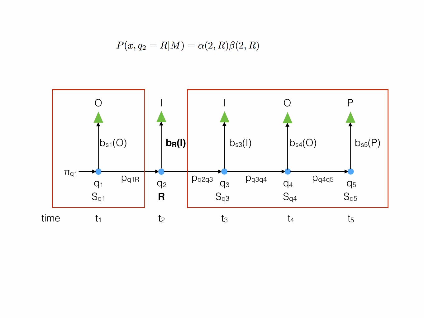
time t1 t2 t3 t4 t5

q1 q2 q3 q4 q5

O I I O P

Sq1 R Sq3 Sq4 Sq5

bs1(O) bR(I) bs3(I) bs4(O) bs5(P)

pq1R pq2q3 pq3q4 pq4q5πq1

time t1 t2 t3 t4 t5

q1 q2 q3 q4 q5

O I I O P

Sq1 RSq2 Sq4 Sq5

bs1(O) bR(I)bs3(I) bs4(O) bs5(P)

pq1q2 pq2R pq3q4 pq4q5πq1

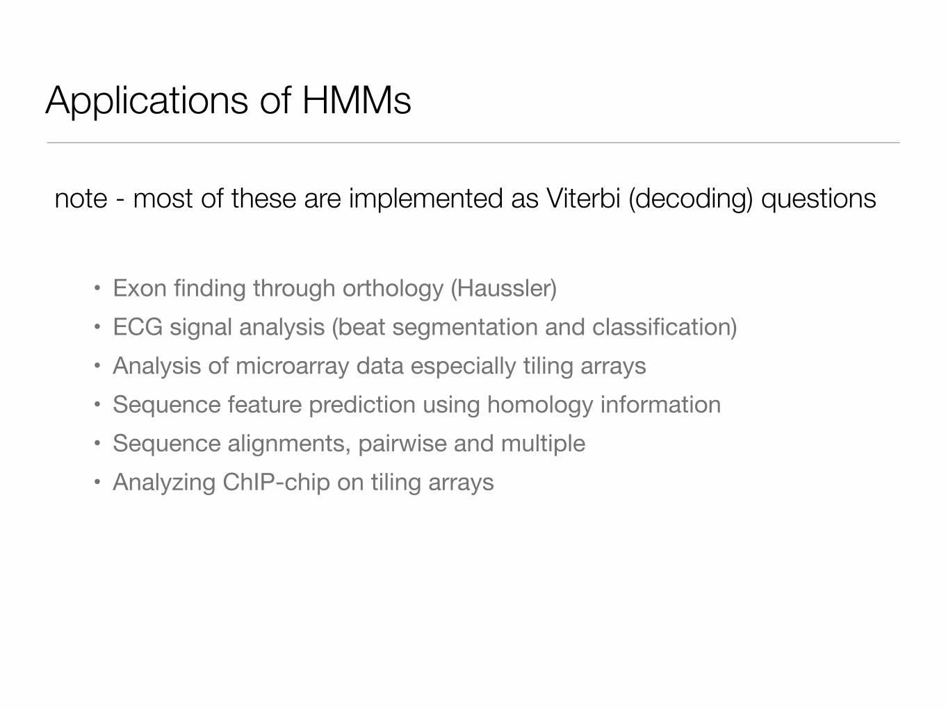
Applications of HMMs

• Exon finding through orthology (Haussler)• ECG signal analysis (beat segmentation and classification)• Analysis of microarray data especially tiling arrays• Sequence feature prediction using homology information• Sequence alignments, pairwise and multiple• Analyzing ChIP-chip on tiling arrays

note - most of these are implemented as Viterbi (decoding) questions

Finding genes

The first gene finders were for prokaryotesNo intronsDistinct and known signals

GLIMMER (1998, Salzberg et al.) was an early gene-finding program and was very successful

Only for prokaryotes (first version)Tested on relatively short sequences

GENSCAN (1997)

• GENSCAN (Burge and Karlin) was a huge breakthrough in eukaryotic gene-finding, and is still used

• How is it different?• Assumes that the input sequence can have no genes, one gene,

multiple genes, or parts of genes• Models all known aspects of a eukaryotic gene• Uses general 3-periodic inhomogeneous fifth-order Markov model of

coding regions• Does not use specific models of protein structure or database

homology

GENSCAN — MDD

Maximal Dependence DecompositionNeed aligned set of several hundred signal sequencesUse conditional probabilities to capture the most significant dependencies between positionsCalculate χ2 for each pair of positions to detect dependencies

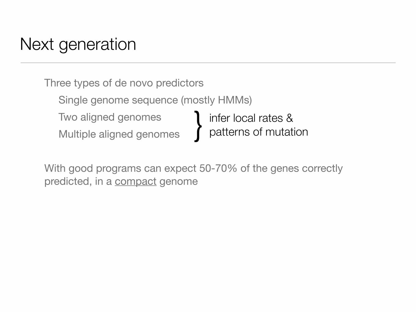
Next generation

Three types of de novo predictorsSingle genome sequence (mostly HMMs)Two aligned genomesMultiple aligned genomes

With good programs can expect 50-70% of the genes correctly predicted, in a compact genome

infer local rates & patterns of mutation}

Next generation

Dual-genome predictors

• Assume that functional regions are more conserved• SLAM (HMM) - uses joint probability for sequence alignment and gene

structure to define types of alignments seen in coding vs noncoding sequence

• More powerful approaches use HMM and dynamic programming• Problem: in closely related species most of the conserved sequences are

noncoding

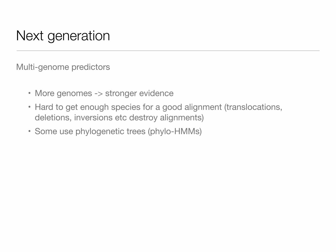
Next generation

Multi-genome predictors

• More genomes -> stronger evidence• Hard to get enough species for a good alignment (translocations,

deletions, inversions etc destroy alignments)• Some use phylogenetic trees (phylo-HMMs)

HMM for copy number variation

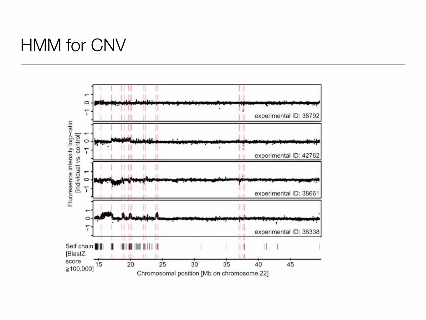
HMM for CNV

detecting pieces of immunoglobulin rearrangements

• infections, neoplasms can stimulate B cell development and antibody production

• antibody production & diversification involves rearranging V(D)J segments of genes

• given an immunoglobulin, what V,D,J segments did it come from?

CpG islands

the CG dinucleotide is extraordinarily underrepresented in vertebrate genomes (about 1/5 the expected frequency)remaining CG dinucleotides cluster in “islands”highly regulatory regions in eukaryotic genomesoverall human genome C+G content is ~42%; CpG island is ~65%

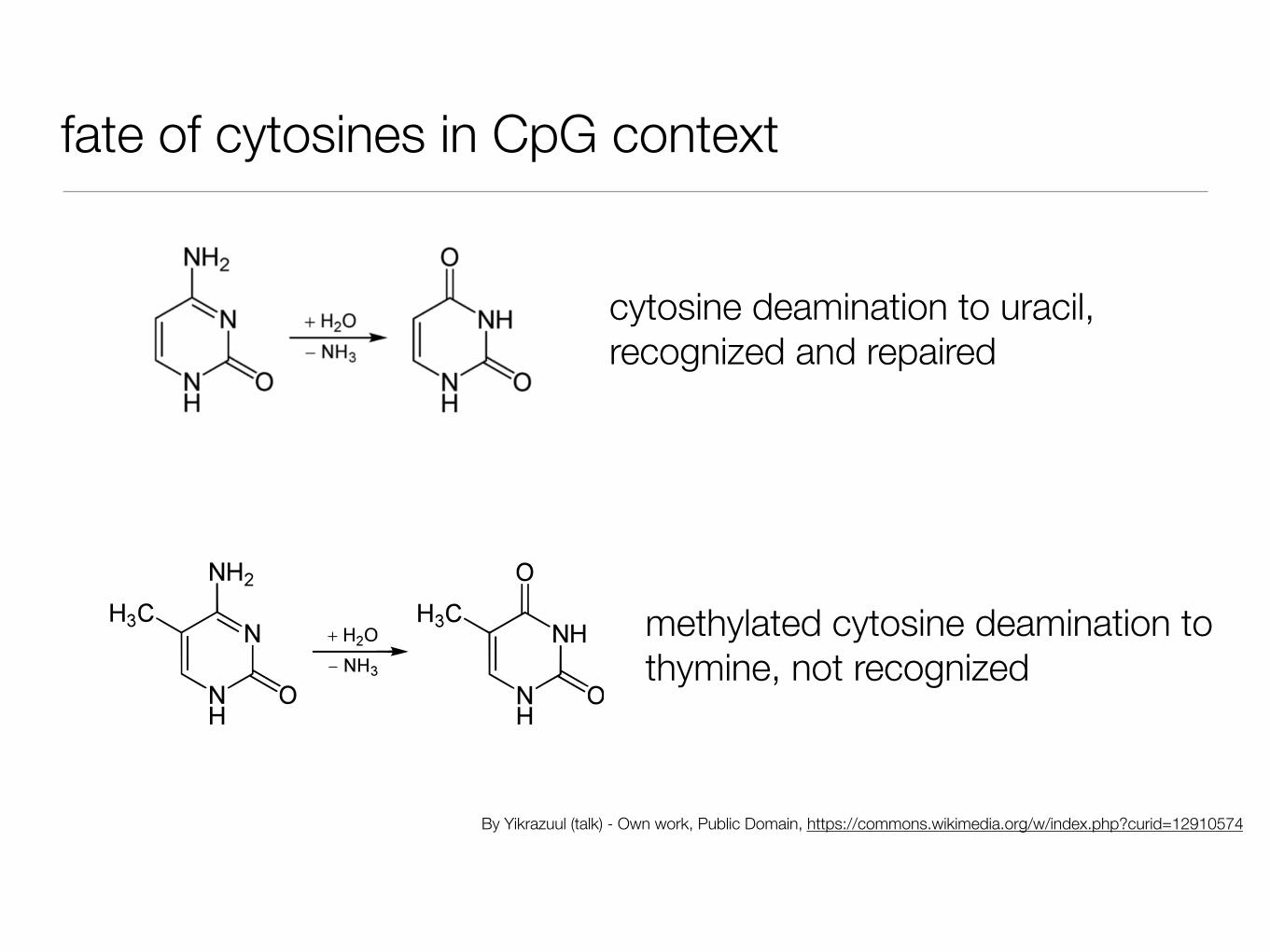
fate of cytosines in CpG context

By Yikrazuul (talk) - Own work, Public Domain, https://commons.wikimedia.org/w/index.php?curid=12910574

cytosine deamination to uracil, recognized and repaired

methylated cytosine deamination to thymine, not recognized

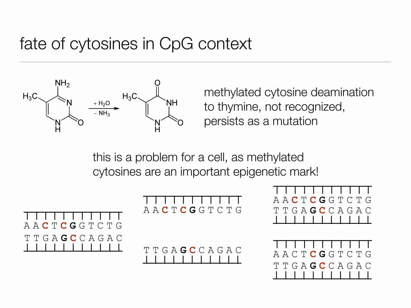
fate of cytosines in CpG context

methylated cytosine deamination to thymine, not recognized, persists as a mutation

this is a problem for a cell, as methylated cytosines are an important epigenetic mark!

A A C T C G G T C T GT T G A G C C A G A C

A A C T C G G T C T G

T T G A G C C A G A C

T T G A G C C A G A CA A C T C G G T C T G

A A C T C G G T C T GT T G A G C C A G A C

CpG islands

200+ nucleotides longG+C content > 50%observed/expected CpG ratio > 0.6

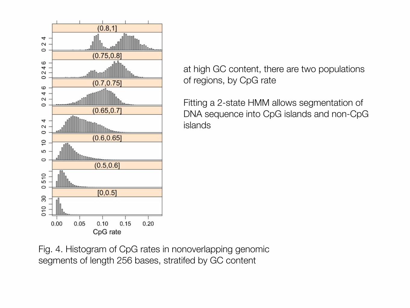
Fig. 4. Histogram of CpG rates in nonoverlapping genomic segments of length 256 bases, stratifed by GC content

at high GC content, there are two populations of regions, by CpG rate

Fitting a 2-state HMM allows segmentation of DNA sequence into CpG islands and non-CpG islands