Basin Analysis 2011-GE-56

1 | P a g e

Figure 1.1 Corel Draw

LAB#01

INTRODUCTION TO BASIN ANALYSIS

1. STATEMENT:

To draw the stratigraphic sequence of different wells by using corel draw

2. SCOPE:

- Using corel draw we correlate the stratigraphy and find the relative ages of different

lithologies.

- The data can be saved in a large no. of extensions.

3. THEORY:

3.1. COREL DRAW:

Corel Corporation developed and released a software program called Corel draw,

a vector graphics editor. The software is more of a graphics suite than just a single, simple

program, providing many features for users to edit graphics, including contrast adjustment, color

balancing, adding special effects like borders to images, and it is capable of working with

multiple layers and multiple pages.

3.2. HISTORY OF COREL DRAW:

In 1987, Corel hired software engineers Michel Bouillon and Pat Beirne to develop a vector-

based illustration program to bundle with their desktop publishing systems. That program,

CorelDraw, was initially released in 1989. CorelDraw 1.x and 2.x runs under Windows 2.x and

Basin Analysis 2011-GE-56

2 | P a g e

3.0. CorelDraw 3.0 came into its own with Microsoft's release of Windows 3.1. The inclusion

of TrueType in Windows 3.1 transformed CorelDraw into a serious illustration program capable

of using system-installed outline fonts without requiring third-party software such as Adobe

Type Manager; paired with a photo editing program (Corel Photo-Paint), a font manager and

several other pieces of software, it was also part of the first all-in-one graphics suite.

3.3. FEATURES OF COREL DRAW:

EXPLANATION OF TOOLS:

- PICK TOOL:

Toll it serves to select or select objects

- SHAPE TOOL:

This tool serves to edit a line or object to the manipulation point

- CROP TOOL:

This tool serves to remove the unwanted part on the object

- ZOOM TOOL:

This tool serves to alter the document window corel we are open

Basin Analysis 2011-GE-56

3 | P a g e

- FREEHAND TOOL:

This tool serves to draw a curve (a curve) and a straight line segment. Freehand may be:

Point line tool: This tool serves to draw a straight line from one point to one point to another

Bezier tool: this tool serves to draw a curved line segment at a time

- SMART FILL TOOL:

This tool serves to make objects from overlapping areas

- RECTANGLE TOOL:

This tool serves to draw rectangles or squares simply by drag and click your mouse

- ELLIPSE TOOL:

This tool serves to draw an ellipse and a circle just by drag and click your mouse

- POLYGON TOOL:

This tool serves to draw a square shape a lot, just by drag and click the mouse

- BASIC SHAPES TOOL:

This tool serves to accelerate the process of drawing a triangle, circle, cylinder, heart, and

many other forms

- TEXT TOOL:

This tool is used to make paper in the drawing area either artistic or description

- TABLE TOOL:

This tool serves to create a table, select and edit table

- BLEND TOOL:

This tool serves to unify the object by creating a lot of objects and colors are housed in the

center

4. STRATIGRAPHIC CORRELATION:

The method of using similarities between geologic units to extend information about geologic

sequences over large geographic areas is called correlation. In lithologic correlation, a unit is

recognized by its lithology (rock type) or a sequence of lithologies.

Basin Analysis 2011-GE-56

4 | P a g e

Figure 1.2 Correlation of US Wells

4.1. TYPES OF CORRELATION:

A) TIME CORRELATION:

Matching of rocks deposited at the same time (e.g. Mesozoic sedimentary rocks in the U.S. with

Mesozoic sedimentary rocks in Mexico). Time correlation requires the use of index fossils to

demonstrate rocks were deposited at the same time.

B) LITHOLOGIC CORRELATION:

Matching rocks of the same character from one place to another. Usually not as accurate as time

correlation, but easier. Doesn't require index fossils, but lithologic correlation may not correlate

rocks deposited at the same time.

4.2. IMPORTANCE OF CORRELATION:

Correlation tells us about:

Sea level changes:

- Transgression

- Regression

Extend of the reservoir

5. APPLICATIONS OF COREL DRAW IN GEOLOGICAL ENGINEERING:

Corel draw can be used in geological engineering for:

- Drawing the stratigraphy of different wells

- Correlation of different stratigraphic beds

- Finding Reservoir and source rock

- Elevation and depression of an area

- 3D Model of an area

REFRENCES:

http://en.wikipedia.org/wiki/CorelDRAW

http://www.computerhope.com/jargon/c/coreldraw.htm

http://homepage.usask.ca/~mjr347/prog/geoe118/geoe118.040.html

http://petrowiki.org/Gamma_ray_logs

Basin Analysis 2011-GE-56

5 | P a g e

http://tool-coreldraw.blogspot.com/2013/03/name-and-function-toolbox-coreldraw.html

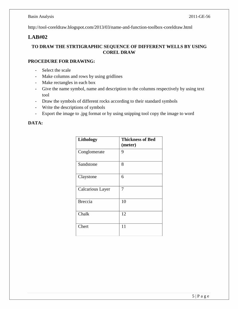
LAB#02

TO DRAW THE STRTIGRAPHIC SEQUENCE OF DIFFERENT WELLS BY USING

COREL DRAW

PROCEDURE FOR DRAWING:

- Select the scale

- Make columns and rows by using gridlines

- Make rectangles in each box

- Give the name symbol, name and description to the columns respectively by using text

tool

- Draw the symbols of different rocks according to their standard symbols

- Write the descriptions of symbols

- Export the image to .jpg format or by using snipping tool copy the image to word

DATA:

Lithology Thickness of Bed

(meter)

Conglomerate 9

Sandstone 8

Claystone 6

Calcarious Layer 7

Breccia 10

Chalk 12

Chert 11

Basin Analysis 2011-GE-56

6 | P a g e

DESCRIPTION OF THE ROCKS:

LAB#03

Basin Analysis 2011-GE-56

7 | P a g e

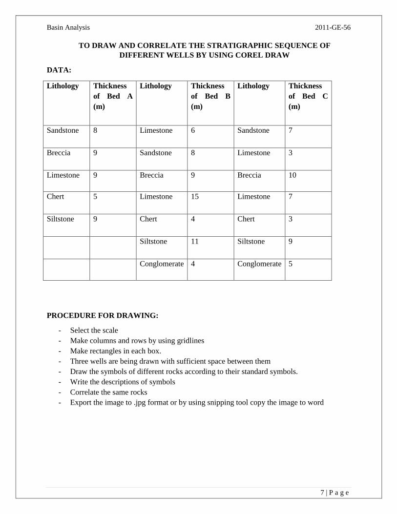
TO DRAW AND CORRELATE THE STRATIGRAPHIC SEQUENCE OF

DIFFERENT WELLS BY USING COREL DRAW

DATA:

Lithology Thickness

of Bed A

(m)

Lithology Thickness

of Bed B

(m)

Lithology Thickness

of Bed C

(m)

Sandstone 8 Limestone 6 Sandstone 7

Breccia 9 Sandstone 8 Limestone 3

Limestone 9 Breccia 9 Breccia 10

Chert 5 Limestone 15 Limestone 7

Siltstone 9 Chert 4 Chert 3

Siltstone 11 Siltstone 9

Conglomerate 4 Conglomerate 5

PROCEDURE FOR DRAWING:

- Select the scale

- Make columns and rows by using gridlines

- Make rectangles in each box.

- Three wells are being drawn with sufficient space between them

- Draw the symbols of different rocks according to their standard symbols.

- Write the descriptions of symbols

- Correlate the same rocks

- Export the image to .jpg format or by using snipping tool copy the image to word

Basin Analysis 2011-GE-56

8 | P a g e

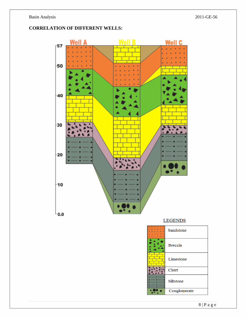
CORRELATION OF DIFFERENT WELLS:

Basin Analysis 2011-GE-56

9 | P a g e

LAB#04

4.1. STATEMENT:

DRAW STRATIGRAPHIC SEQUENCE OF LOWER INDUS BASIN BY USING COREL

DRAW

4.2. SCOPE:

- To get information about the stratigraphic layers of indus basin so that the petroleum reserves

can be identified

- Sequence of deposition is very important for the exploration of petroleum reserves

4.3. THEORY:

4.3.1. SEDIMENTARY BASIN:

Sedimentary basins are regions of the earth of long-term subsidence creating accommodation

space for infilling by sediments. The subsidence results from the thinning of underlying crust,

sedimentary, volcanic, and tectonic loading, and changes in the thickness or density of adjacent

lithosphere. Sedimentary basins occur in diverse geological settings usually associated with plate

tectonic activity.

4.3.2. BASIN MAP OF PAKISTAN:

Figure 4.1

Basin Analysis 2011-GE-56

10 | P a g e

Figure 4.2

4.3.3. MAJOR SEDIMENTARY BASINS OF PAKISTAN:

According to Ministry of petroleum of Pakistan there are 10 basins in Pakistan.

1) Kohat Potwar Basin

2) Central Indus Platform Basin

3) Lower Indus Platform Basin

4) Sulaiman Fold Belt Basin

5) Kirthar Fold Belt Basin

6) Northern Punjab Basin

7) Pishin Fold Belt Basin

8) Balochistan Fold Belt Basin

9) Makran Fold Belt Basin

10) Offshore Indus Basin

However some authers say that there are only three major basins:

Indus Basin

balochistan Basin

Axial Belt

4.3.4. INDUS BASIN OF PAKISTAN:

The catchment area of Indus River is unique and includes 7 worlds’ highest ranking peaks such

as K-2 (28,253 feet), Nanga Parbat (26,600 feet) and Rakaposhi (25,552 feet) in addition to 7

glaciers including Siachin, Hispar, Biafo, Batura, Barpu and Hopper. Indus River originates from

the north side of the Himalayas at Kaillas Parbat in Tibet having altitude of 18000 feet. One of

the important Eastern River draining into the Indus River System is Jhelum River which

originates from Pir Panjal and flows parallel to the Indus at an elevation of 5500 feet. The length

of the main river from the most remote point to the outlet has been estimated to be about 260

miles. Basin shape is numerically calculated with the help of Horton's method and estimated as

0.190. This value indicates an irregular basin with comparatively moderate peaks. Using

different methods commonly used in drainage basin studies, various dimensionless catchment

parameters, useful in predicting inflow in a river have been estimated for the basin.

Basin Analysis 2011-GE-56

11 | P a g e

Figure 2.3

4.3.5. STRATIGRAPHIC LOWER INDUS BASIN:

The Lower Indus Basin (Pakistan) covers an area of about 400,000 km2. It contains several oil

and gas discoveries, the largest of which is the Sui gas field (discovered in 1952, with estimated

initial recoverable reserves of 8.624 tcf gas).

The basin lies on the western margin of the Indian Plate and deepens steeply to the west. Cross

sections of the basin are shown in Kadri (1995). Its eastern margin is formed by the Punjab Shelf

and Thar Platform, which are separated by the Jocobabad and Mari-Kandkhot Highs that lie

partly in India. The central deepest part of the basin is known as the Sulaiman Depression in the

northern part of the basin and the Karachi Trough in the south. The northern and central parts of

its western margin are marked by the thrust faults of the Sulaiman and Kirthar fold belts. To the

south, the basin extends offshore. Shown in fig 4.3.

The Thar Platform contains well developed Early to Middle Cretaceous sands that form the

reservoirs of all the gas fields in this region. The Punjab Shelf contains some major stratigraphic

pinchouts. The Sulaiman depression contains some buried anticlines. The Karachi Trough, which

opens up into the Arabian Sea, contains large numbers of anticlines, some of which form gas

fields.

Basin Analysis 2011-GE-56

12 | P a g e

4.4. LOWER INDUS BASIN FORMATION AND LITHOLOGY MAP:

Basin Analysis 2011-GE-56

13 | P a g e

REFRENCES:

http://en.wikipedia.org/wiki/Sedimentary_basin

http://decarboni.se/publications/regional-assessment-potential-co2-storage-indian-

subcontinent/appendix-3-brief

(www.mpnr.gov.pk)

http://en.allexperts.com/q/Geology-1359/2012/4/sedimentary-basins-pakistan.htm

http://en.allexperts.com/q/Geology-1359/2011/1/Geological-Basins-Pakistan-1.htm

Basin Analysis 2011-GE-56

14 | P a g e

LAB#05

5.1. STATEMENT:

TO CORRELATE THE GIVEN LOG DATA AND IDENTIFY THE DEPOSITIONAL

ENVIRONMENT

5.2. SCOPE:

- Sea level changes can be calculated

- Lithology can also be fined

5.3. RELATED THEORY:

5.3.1. TRANSGRESSION:

Transgression is a geologic event during which sea level rises relative to the land and the

shoreline moves toward higher ground, resulting in flooding.

5.3.2. REGRESSION:

The opposite of transgression is regression, in which the sea level falls relative to the land and

exposes former sea bottom.

5.3.3. CAUSES OF LEVEL CHANGES:

Sea levels change for three main reasons:

1) As water warms and cools it expands and contracts.

2) The amount of water contained as ice on land surfaces changes over time.

3) The Earth’s surface is dynamic and can move vertically.

The first two reasons are directly caused by global temperature changes. More specifically

transgressions and regressions may be caused by tectonic events such as orogenies,

severe climate change such as ice ages or isostatic adjustments following removal of ice or

sediment load.

5.3.4. APPLICATIONS OF TRANSGRESSION AND REGRESSION:

The study of strata deposited along continental margins under the influence of cyclical Earth

processes such as eustatic sea level change is a branch of stratigraphy called sequence

stratigraphy. Development of this geologic sub discipline in the early 1970s is largely attributed

to petroleum industry researchers who first used seismic reflection profiles to map the

distribution of oil and gas bearing strata in sedimentary basins. Because relative sea level change

determines the location and geometry of these oil-bearing strata along continental margins,

sequence stratigraphy is a powerful predictive tool for oil and gas exploration.

Basin Analysis 2011-GE-56

15 | P a g e

TABLE#01

Lithology Thickness of Bed A

(m)

Thickness of Bed B

(m)

Shale 5 -

Transgression Siltstone 7 6.5

Conglomerate 4 5

Sandstone - 11

Regression Coal - 4.5

Limestone 8 7

Siltstone 6.5 4.5

Transgression Shale 4 3.5

Breccia 7.5 -

WELL A WELL B

Basin Analysis 2011-GE-56

16 | P a g e

TABLE#02

Formation Well (A) Well

(B)

Well (C) Remarks

Limestone 5 4 2.5

Transgression Shale 8 8 5.5

Sandstone 6.5 8 4

Coal - - 3

Regression Sandstone - - 4

Siltstone 6.5 5 4

Transgression Dolomite 9 7 4.5

Sandstone - 3 7

WELL A

WELL B

WELL C

Basin Analysis 2011-GE-56

17 | P a g e

REFRENCES:

http://en.wikipedia.org/wiki/Marine_transgression

http://www.dnrec.delaware.gov/coastal/Documents/SLR%20Advisory%20Committee/Adapt

Engage/3WhatCausesSeastoRise.pdf

http://www.bookrags.com/research/marine-transgression-and-marine-reg-woes-

02/#gsc.tab=0

Basin Analysis 2011-GE-56

18 | P a g e

Figure 6.3

LAB#06

6.1. STATEMENT:

INTRODUCTION TO SURFER SOFTWARE AND ITS APPLICATIONS IN THE

FIELD OF GEOLOGICAL ENGINEERING

6.2. SCOPE:

- It is used for volume based and surface based analysis

- Used for analyzing magnetic resonance imaging

6.3. THEORY:

6.3.1. SURFER:

Surfer is a full-function 3D visualization, contouring and surface modeling package that runs

under Microsoft Windows. Founded in 1983, Golden Software is one of the world's oldest

software companies, and the first to market three-dimensional surface and contour mapping

applications for the PC.

Basin Analysis 2011-GE-56

19 | P a g e

6.3.2. HISTORY OF SURFER:

Patrick Madison, a CSM computer science instructor, and Dan Smith, a graduate student, began

a partnership in 1983 with the development of a printer interface language that took advantage of

the full resolution available to dot-matrix printers. Their first commercial program, PlotCall,

transformed plotter instructions into dot-matrix instructions compatible with over 20 commercial

printers. This opened the computer graphing and mapping market to the wider arena of users

with inexpensive commercial printers. Between 1985 and 1986 the company released

two DOS applications: Surfer, surface and contour mapping program, and Grapher, a

spreadsheet-plotting application. In 1990 it released its first Windows program: Map Viewer.

Their next product, Didger was released in 1996. Their most recent

programs, Strater and Voxler began shipping in 2004 and 2006.

Applications of Surfer in Geological Engineering:

Surfer is used extensively for

Terrain modeling

Bathymetric modeling

Landscape visualization

Surface analysis

Contour mapping

Watershed

3d surface mapping

Gridding

Volumetric

It has major role in exploration purposes in petroleum industry. Scientists and engineers

worldwide have discovered Surfer's power and simplicity.

6.3.3. FEATURES OF SURFER SOFTWARE:

- Contour Map

- Base Map

- Post Map

- 3D Surface Map

- 3D Wireframe Map

- Image Map

- Work Sheets

- Map Projections

Basin Analysis 2011-GE-56

20 | P a g e

Figure 6.4 Contour Map

6.3.4. COMMANDS USED IN SURFER:

GRID FILES:

Grid files are created using the Grid | Data command. The Grid | Data command requires data in

three columns: one column containing X data, one column containing Y data, and one column

containing Z data.

NODE:

The grid node editor opens a grid file for editing. Nodes display with a black “+”, blanked nodes

with a blue “x”, and the active node is highlighted with a red diamond.

Break line:

Break lines are used when gridding to show discontinuity in the grid. A breakline is a three

dimensional .BLN boundary file that defines a line with X, Y, and Z values at each vertex.

Overlay Map:

If two maps already existed, a map layer can be dragged to a different map object in the Object

Manager. Alternatively, select both maps and click the Map | Overlay Maps command. All

selected map layers are moved to a single map object.

6.3.5. CONTOUR MAP:

Surfer contour maps give you full control over all map parameters. You can accept the Surfer

intelligent defaults to automatically create a contour map, or double-click a map to easily

customize map features. Display contour maps over any contour range and contour interval, or

specify only the contour levels you want to display on the map. And with Surfer you can add

color fill between contours to produce dazzling displays of your maps, or produce gray scale fills

for dramatic black and white printouts.

Basin Analysis 2011-GE-56

21 | P a g e

Figure 6.5 3D Surface Map

Figure 6.6 Vector Map

6.3.6. 3D SURFACE MAP:

The 3D surface map uses shading and color to emphasize your data features. Change the

lighting, display angle and tilt with a click of the mouse. Overlay several surface maps to

generate informative block diagrams.

6.3.7. VECTOR MAP:

Instantly create vector maps in Surfer to show direction and magnitude of data at points on a

map. You can create vector maps from information in one grid or two separate grids. The two

components of the vector map, direction and magnitude, are automatically generated from a

single grid by computing the gradient of the represented surface. At any given grid node, the

direction of the arrow points in the direction of the steepest descent. The magnitude of the arrow

changes depending on the steepness of the descent.

Basin Analysis 2011-GE-56

22 | P a g e

Figure 6.7 Post Map

Figure 6.8 Base Map

6.3.8. POST MAP:

Post maps show X,Y locations with fixed size symbols or proportionally scaled symbols of any

color. Create post maps independent of other maps on the page, or overlay the posted points on a

base, contour, vector, or surface map. For each posted point, specify the symbol and label type,

size, and angle. Also create classed post maps that identify different ranges of data by

automatically assigning a different symbol or color to each data range. Post your original data

point locations on a contour map to show the distribution of data points on the map, and to

demonstrate the accuracy of the gridding methods you use.

6.3.9. BASE MAP:

Surfer can import maps in many different formats to display geographic information. You can

combine base maps with other maps in map overlays, or can create stand-alone base maps

independent of other maps on the page. You can load any number of base maps on a page. It is

easy to overlay a base map on a contour or surface wireframe map, allowing you to display

geographic information in combination with the three dimensional data.

Basin Analysis 2011-GE-56

23 | P a g e

6.4. REFRENCES:

http://en.wikipedia.org/wiki/Golden_Software

http://www.ssg-surfer.com/html/surfer_details.html

http://www.geomem.com/products/6/surfer.html

Basin Analysis 2011-GE-56

24 | P a g e

LAB#07

7.1. STATEMENT:

BY USING THE LOCATIONS OF DIFFERENT WELLS AD THICKNESS OF GIVEN

FORMATIONS DRAW MAPS OF EACH WELL ON SURFER AND GIVE

INTERPRETATION OF EACH WELL

7.2. GIVEN DATA:

Well

no.

Longitude

Latitude

Thickness of Formation

A B C D E F

1 71.3942 29.112 - - 224 19 317 81

2 72.154 29.2286 817 93 113 - - -

3 71.9303 30.8227 50 89 129 - - 31

4 71.6661 28.1761 140 141 29 - - 230

5 72.1575 30.9958 - - 56 - - 34

6 70.2361 28.1474 - - - - 1306 101

7 71.9507 31.4694 406.5 210 - - - -

8 72.6982 28.9754 251 797 - - - -

9 70.8532 28.032 - - 294 22 856 27

10 71.5203 31.1936 - - 15 - 201 21

11 72.3663 29.9771 906 120 - - - -

12 72.5698 29.2442 1143 99 - - - -

13 71.9291 30.523 - - 134 - -- 43

14 71.9594 30.6841 - - 129 - - 45

15 72.0173 30.3448 - - 127 - - 40

16 71.9277 30.5393 222 306 103 - - 42

17 71.8259 31.2321 - - 24 - - -

18 71.7398 28.5952 332 50 31 161 161 76

19 72.2311 30.2556 - - 121 - - 39

Basin Analysis 2011-GE-56

25 | P a g e

7.3. PROCEDURE:

For contour map:

1) Copy the data from excel file to the New work sheet in the surfer including Longitude,

latitude and thickness and save the file as .bln Extension file.

2) Go to the plot sheet and click on the Grid

and data, insert the .bln file and a grid

file is generated.

3) Now click on the contour map and insert the same grid file that is generated.

Basin Analysis 2011-GE-56

26 | P a g e

4) A contour map is drawn. Where its colour and shape can be changed in its properties.

5) For post map:

The same procedure is done without making its grid file and the .bln file would have well no. in

its sheet file.

6) Once the post map is drawn, drag the post before the contour map (overlay). Now delete the

map (extra).

Basin Analysis 2011-GE-56

27 | P a g e

Figure 7.9

7) This is the final result. Where North arrow can be added from symbol and colour and shape

can be changed from properties

7.4. DIFFERENT WELLS:

7.4.1.

WELL A:

Formation=

Limestone

Basin Analysis 2011-GE-56

28 | P a g e

Figure 7.3

Figure 7.10

7.4.2. WELL B:

Formation=

Silty Shale

7.4.3. Well C:

Formation=Breccia

Basin Analysis 2011-GE-56

29 | P a g e

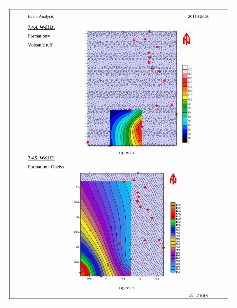
Figure 7.4

Figure 7.5

7.4.4. Well D:

Formation=

Volcanic tuff

7.4.5. Well E:

Formation= Gneiss

Basin Analysis 2011-GE-56

30 | P a g e

Figure 7.6

7.4.6. Well F:

Formation=

Sandstone

7.5. REFRENCES:

- Class Notes

Basin Analysis 2011-GE-56

31 | P a g e

INTERPRETATIONS FROM WELLS

WELL A:

The depocenter lies at the latitude 29.24, longitude 72.6 and thickness is 1143 ft. which shows

that maximum deposition.

WELL B:

The maximum deposition (depocenter) lies at latitude 28.97, longitude 72.69 and the thickness is

797 ft.

WELL C:

The maximum deposition lies at latitude 28.03, longitude 70.85 and max thickness is 224 ft.

WELL D:

The maximum deposition (depocenter) lies at latitude 28.59, longitude 71.73 and the thickness is

161 ft

WELL E:

The maximum deposition lies at latitude 28.14, longitude 70.23 and thickness is 1306 ft.

WELL F:

The maximum deposition lies at latitude 28.17, longitude 71.66 and thickness is 230 ft.

Basin Analysis 2011-GE-56

32 | P a g e

LAB#08

8.1. STATEMENT:

BY USING THE LOCATIONS OF DIFFERENT WELLS AD THICKNESS OF GIVEN

FORMATIONS DRAW MAPS OF EACH WELL ON SURFER AND GIVE

INTERPRETATION OF EACH WELL

8.2. GIVEN DATA:

Well

no.

Longitude

Latitude

Thickness of Formation

A B C D E F

1 71.3942 29.112 - - 224 19 317 81

2 72.154 29.2286 817 93 113 - - -

3 71.9303 30.8227 50 89 129 - - 31

4 71.6661 28.1761 140 141 29 - - 230

5 72.1575 30.9958 - - 56 - - 34

6 70.2361 28.1474 - - - - 1306 101

7 71.9507 31.4694 406.5 210 - - - -

8 72.6982 28.9754 251 797 - - - -

9 70.8532 28.032 - - 294 22 856 27

10 71.5203 31.1936 - - 15 - 201 21

11 72.3663 29.9771 906 120 - - - -

12 72.5698 29.2442 1143 99 - - - -

13 71.9291 30.523 - - 134 - -- 43

14 71.9594 30.6841 - - 129 - - 45

15 72.0173 30.3448 - - 127 - - 40

16 71.9277 30.5393 222 306 103 - - 42

17 71.8259 31.2321 - - 24 - - -

18 71.7398 28.5952 332 50 31 161 161 76

19 72.2311 30.2556 - - 121 - - 39

Basin Analysis 2011-GE-56

33 | P a g e

8.3. PROCEDURE:

- Insert data from the excel to the New work sheet in the surfer, containing longitude, latitude

and thickness of formation and save it as bln. Extension file.

- Now using Grid option make it grid file. A report will be generated

- Now go to the New 3D surface map option and insert the same grid file that is generated. So

the final #d surface map is generated.

Basin Analysis 2011-GE-56

34 | P a g e

8.4. 3D SURFACE MAP OF WELL A:

INTERPRETATIONS:

The depocenter lies at the latitude 29.24o, longitude 72.6

o and thickness is 1143 ft. which shows

that maximum deposition. Also the thickness is very low at latitude 30.82o, longitude 71.93

o and

thickness is 50 ft. There is a gradual increase of thickness in this region.

Figure 8.1 3D Surface Map Of Well A

Basin Analysis 2011-GE-56

35 | P a g e

8.5. 3D SURFACE MAP OF WELL B:

INTERPRETATIONS:

The maximum deposition lies at latitude 28.97o, longitude 72.69

o and the thickness is 797 ft. The

thickness decreases at the latitude 28.59o, longitude 71.73

o and the thickness is 50 ft. There is a

variation of the thickness in this region.

Figure 8.2 3D Surface Map Of Well B

Basin Analysis 2011-GE-56

36 | P a g e

8.6. 3D SURFACE MAP WELL C:

INTERPRETATIONS:

The maximum deposition lies at latitude 28.03o, longitude 70.85

o and max thickness is 224 ft.

The lowest deposition occours at latitude 31.19o, longitude 71.52

o and thickness is 15 ft. There is

not a gradual variation in this region and the thickness increases slowly.

Figure 8.3 3D Surface Map Of Well C

Basin Analysis 2011-GE-56

37 | P a g e

8.7. 3D SURFACE MAP WELL D:

INTERPRETATIONS:

The maximum deposition (Depocenter) lies at latitude 28.59o, longitude 71.73

o and the thickness

is 161 ft. The lowest deposition occours at latitude 29.11o, longitude 71.39

o with thickness of 19

ft. The thickness does’t vary gradually and hence the slope occours in a normal way.

Figure 8.4 3D Surface Map Of Well D

Basin Analysis 2011-GE-56

38 | P a g e

8.8. 3D SURFACE MAP WELL E:

INTERPRETATIONS:

The maximum deposition lies at latitude 28.14o, longitude 70.23

o and thickness is 1306 ft. The

lowest deposition occours at latitude 28.59o, longitude 71.73

o and thickness is 161 ft. There is

not a large gradual variation of thickness.

Figure 8.5 3D Surface Map Of Well E

Basin Analysis 2011-GE-56

39 | P a g e

8.9. 3D SURFACE MAP WELL F:

INTERPRETATIONS:

The maximum deposition lies at latitude 28.17o, longitude 71.66

o and thickness is 230 ft. The

lowest deposition occours at latitude 31.19o, longitude 71.52

o and thickness is 21 ft. There is not

a large gradual variation of thickness.

Figure 8.6 3D Surface Map Of Well F