basic reserving workshop - menu – home (en) · 2014 5,708 10,268 12,699 2015 6,093 11,172 2016...
TRANSCRIPT

BASIC RESERVING WORKSHOP21 August 2017Roger Hayne
Basic Loss Reserving
• Groundwork and Basics– Definitions– Considerations
• Basic Reserving Techniques– Paid Loss Development Method (PLDM)– Incurred Loss Development Method (ILDM)
Definitions
• What is a Loss Reserve?Unpaid amount required to settle all claims, whether reported or not, for which liability exists on a particular accounting date.
• Why are Loss Reserves Important?Needed for accurate evaluation of financial condition & underwriting income
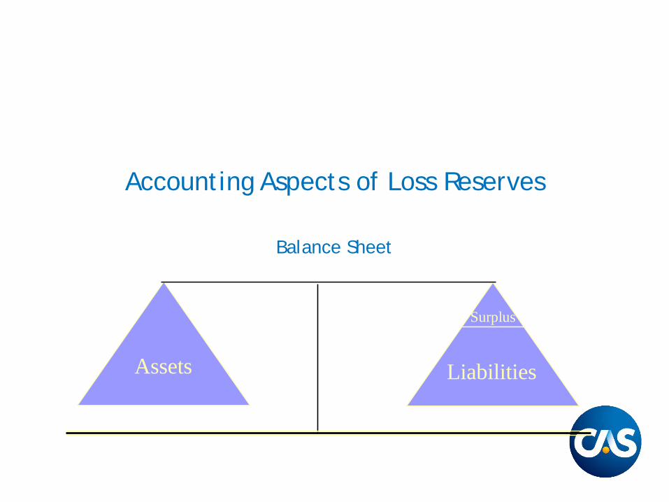
Accounting Aspects of Loss Reserves
Balance Sheet
Assets Liabilities
Surplus
Definitions
• Carried Loss ReserveThe amount shown in a published statement or an internal statement of financial condition.
• Indicated Loss ReserveThe amount that results from the application of a particular loss reserving method.
• Reserve Margin/DeficitThe difference between an indicated loss reserve and a carried loss reserve.
Definitions
• Elements of a Loss Reserve– Incurred But Not Reported (“Pure” IBNR)– Claims in Transit (Reported Not Reserved Yet)– Formula Reserve/Case Reserve– Development on Known Claims– Reopened Claims Reserve
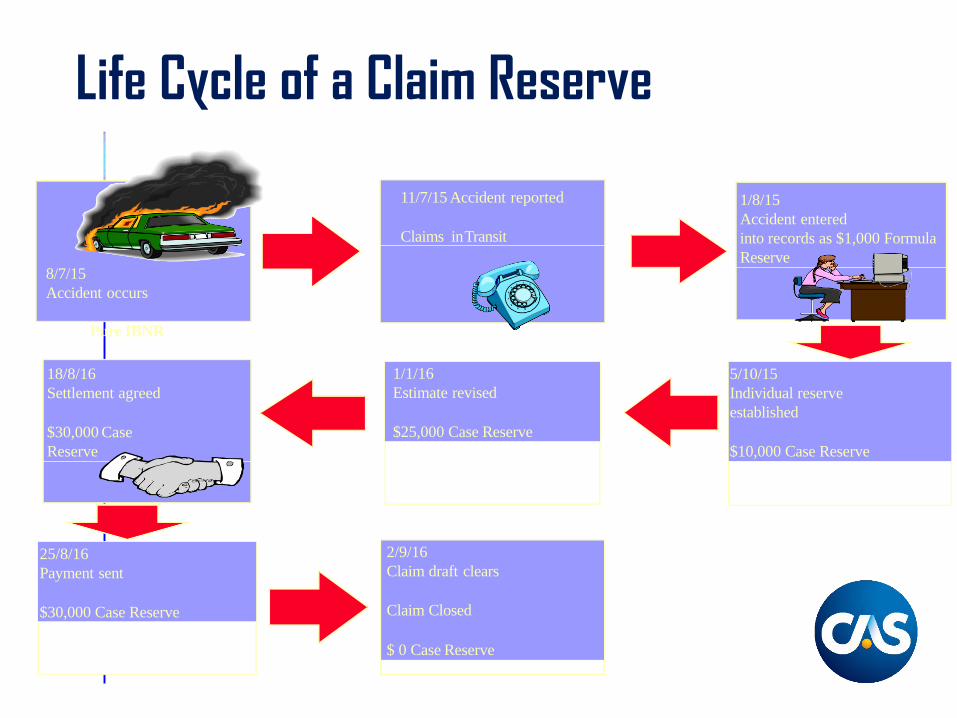
Life Cycle of a Claim Reserve
1/8/15Accident enteredinto records as $1,000 Formula Reserve
11/7/15 Accident reported
Claims inTransit
5/10/15Individual reserve established
$10,000 Case Reserve
1/1/16Estimate revised
$25,000 Case Reserve
18/8/16Settlement agreed
$30,000 Case Reserve
25/8/16Payment sent
$30,000 Case Reserve
2/9/16Claim draft clears
Claim Closed
$ 0 Case Reserve
8/7/15Accident occurs
Pure IBNR
Definitions
• Case Reserves– For specific claim reported but not yet settled– Assigned a value by a claims adjuster or by
formula based on information known for that claim• Bulk + IBNR Reserves
– Reserves for claims not yet reported (“pure” IBNR)– Claims in transit– Development on known claims– Reserves for reopened claims
• Can also include expenses for settling claims
Other Terminology in Use
• Carried Loss Reserve = Unpaid Losses, Outstanding Reserve, Total Reserve
• Indicated Loss Reserve = Unpaid Claim Estimate, Best Estimate, Point Estimate, Actuarial Central Estimate
• Reserve Margin/Deficit = Redundancy/Deficiency• Incurred Losses = Ultimate Losses (incl. IBNR) or
sometimes Reported Losses (excl. IBNR)• Losses may mean Losses and LAE (e.g. Casualty
Loss Reserve Seminar)
Principles
• Actuarially sound reserves– based on estimates– derived from reasonable assumptions– using appropriate methods
• Inherent Uncertainty– a range of reserves can be actuarially sound– true value known only after all claims settled
Principles
• Most appropriate indicated reserve depends on:
– relative likelihood of estimates in range– financial reporting context
Considerations: Data Organization
• Accident Date– The date on which the loss occurred.
• Report Date– The date on which the loss is first reported to the
insurer.
• Recorded Date– The date on which the loss is first entered into
the statistical records of the insurer.
Considerations: Data Organization
• Accounting Date– Defines a group of claims for which liability may
exist.– All claims incurred on or before the accounting
date.
• Valuation Date– Defines the time period for which transactions are
included when evaluating the existing liability.
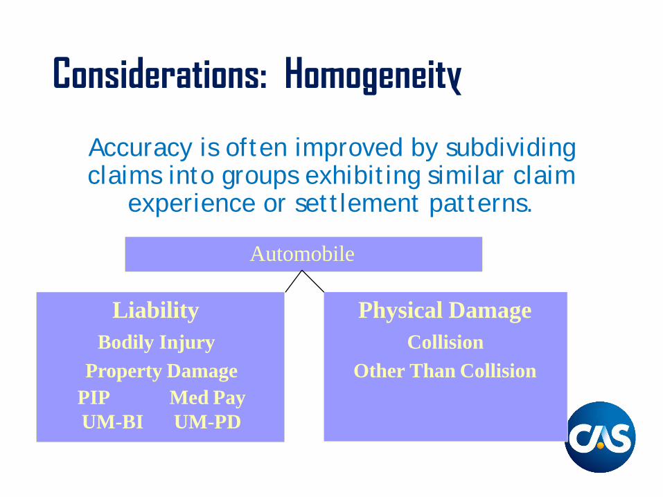
Considerations: Homogeneity
Accuracy is often improved by subdividing claims into groups exhibiting similar claim
experience or settlement patterns.
Automobile
LiabilityBodily Injury
Property DamagePIP Med Pay UM-BI UM-PD
Physical DamageCollision
Other Than Collision
Considerations: Credibility
• A measure of the predictive value that is attached to a body of data.
• A group of claims should be large enough to be statistically reliable.
– May be a point at which subdividing claims will form groups that are too small to provide credible development patterns.
• Use of supplementary data sources– Examples include industry data, countrywide data.

Basic Reserving Techniques: Definitions
• Loss Development– The financial activity on claims from the time they
occur to the time they are eventually settled and paid.
• Triangles– Compiled to measure the changes in cumulative
claim activity over time in order to estimate patterns of future activity.
• Loss Development Factor– The ratio of losses at successive evaluations for a
defined group of claims (e.g. accident year).
Basic Reserving Techniques:Compilation of Paid Loss Triangle
• The losses are sorted by the year in which the accident occurred.
• The payments from inception are summed at the end of each year.
• Losses paid to date are shown on the most recent column (accounting) or diagonal (actuarial).
• Actuarial triangle shows that more recent accident years are at earlier stages of claim life cycle.
• Future development might be similar to historical.
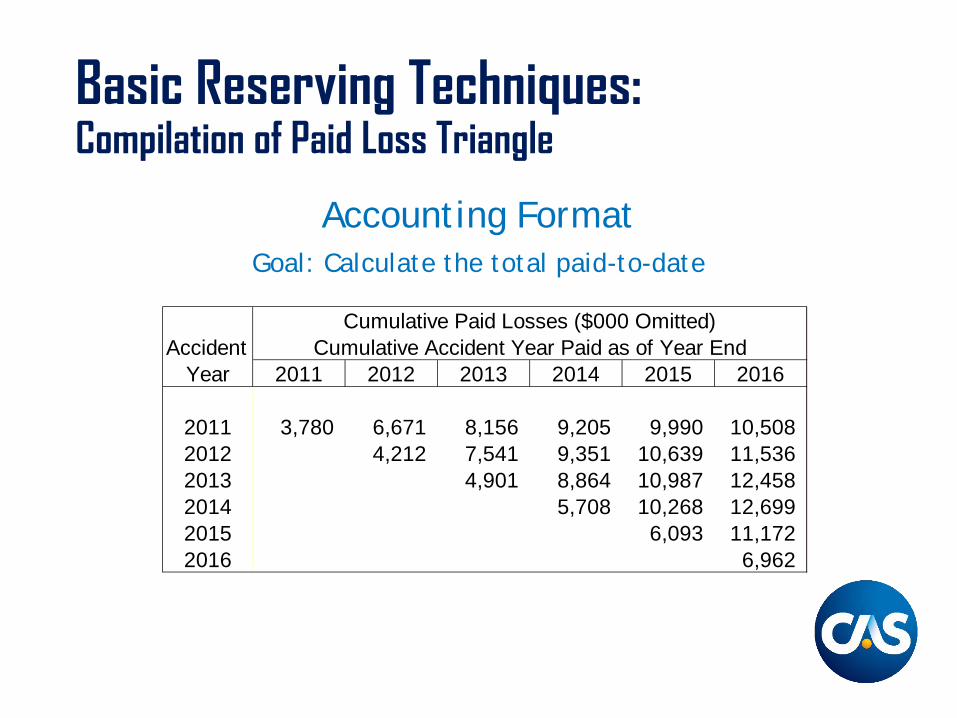
Basic Reserving Techniques:Compilation of Paid Loss Triangle
Accounting FormatGoal: Calculate the total paid-to-date
Cumulative Paid Losses ($000 Omitted)Accident Cumulative Accident Year Paid as of Year End
Year 2011 2012 2013 2014 2015 2016
2011 3,780 6,671 8,156 9,205 9,990 10,508 2012 4,212 7,541 9,351 10,639 11,536 2013 4,901 8,864 10,987 12,458 2014 5,708 10,268 12,699 2015 6,093 11,172 2016 6,962
Basic Reserving Techniques:Compilation of Paid Loss Triangle
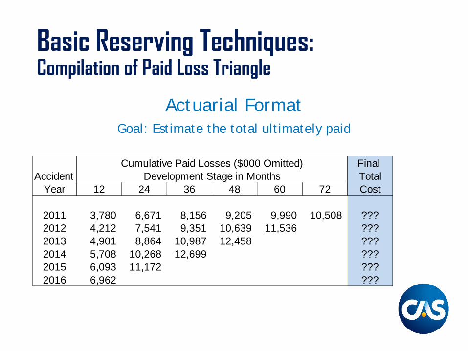
Actuarial FormatGoal: Estimate the total ultimately paid
Cumulative Paid Losses ($000 Omitted) Final Accident Development Stage in Months Total
Year 12 24 36 48 60 72 Cost
2011 3,780 6,671 8,156 9,205 9,990 10,508 ???2012 4,212 7,541 9,351 10,639 11,536 ???2013 4,901 8,864 10,987 12,458 ???2014 5,708 10,268 12,699 ???2015 6,093 11,172 ???2016 6,962 ???
Basic Reserving Techniques:Paid Loss Development Factors
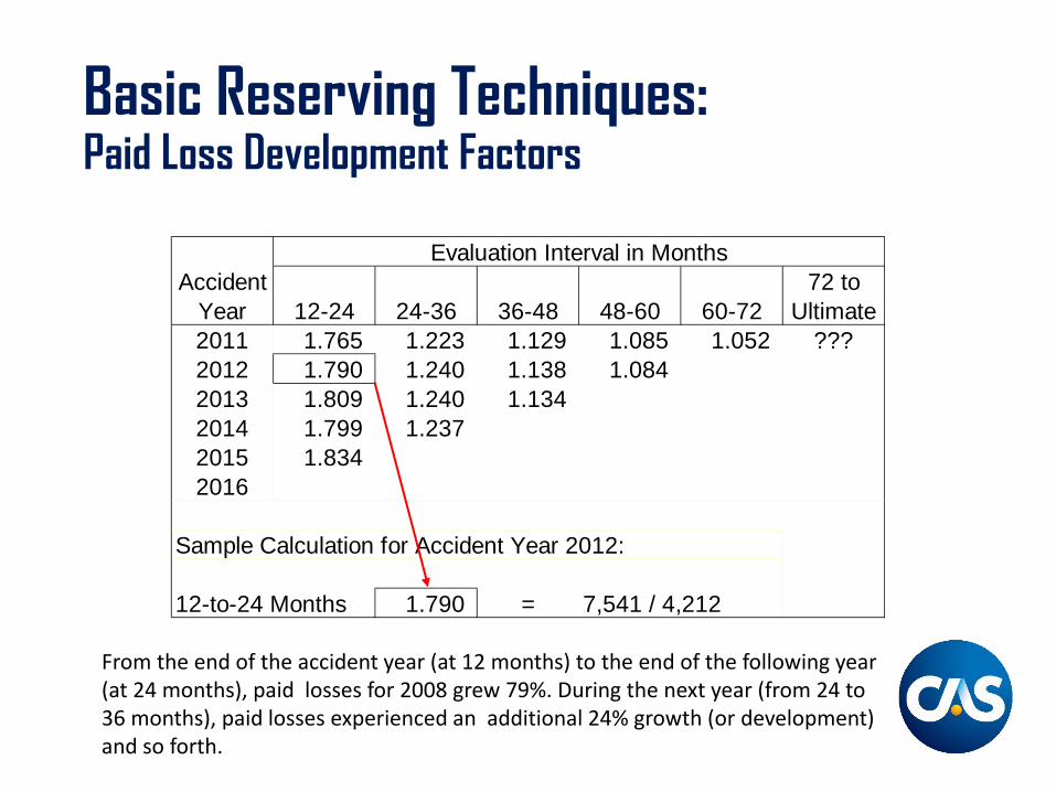
From the end of the accident year (at 12 months) to the end of the following year (at 24 months), paid losses for 2008 grew 79%. During the next year (from 24 to 36 months), paid losses experienced an additional 24% growth (or development) and so forth.
Evaluation Interval in MonthsAccident 72 to
Year 12-24 24-36 36-48 48-60 60-72 Ultimate2011 1.765 1.223 1.129 1.085 1.052 ???2012 1.790 1.240 1.138 1.084 2013 1.809 1.240 1.134 2014 1.799 1.237 2015 1.834 2016
Sample Calculation for Accident Year 2012:
12-to-24 Months 1.790 = 7,541 / 4,212
Basic Reserving Techniques:Compilation of Paid Loss Triangle
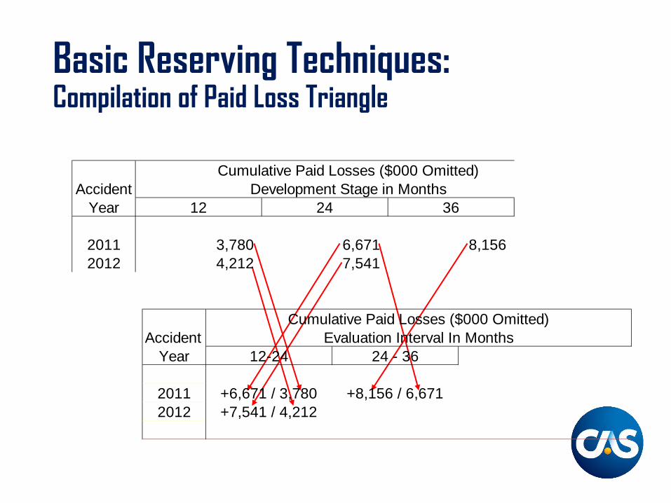
Cumulative Paid Losses ($000 Omitted)Accident Development Stage in Months
Year 12 24 36
2011 3,780 6,671 8,156 2012 4,212 7,541
Cumulative Paid Losses ($000 Omitted)Accident Evaluation Interval In Months
Year 12-24 24 - 36
2011 +6,671 / 3,780 +8,156 / 6,6712012 +7,541 / 4,212
Basic Reserving Techniques:Compilation of Paid Loss Triangle
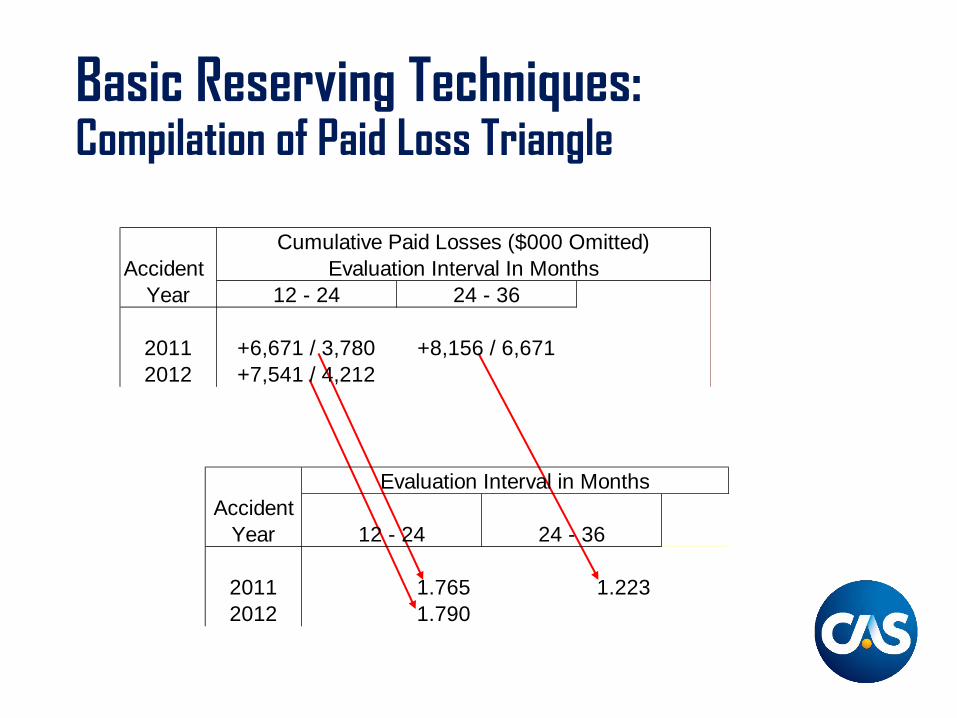
Cumulative Paid Losses ($000 Omitted) Accident Evaluation Interval In Months
Year 12 - 24 24 - 36
2011 +6,671 / 3,780 +8,156 / 6,6712012 +7,541 / 4,212
Evaluation Interval in MonthsAccident
Year 12 - 24 24 - 36
2011 1.765 1.223 2012 1.790
Basic Reserving Techniques:Paid Loss Development Factors
Loss Development Factors (LDFs) are also known as:
– Age-to-Age Factors– Link Ratios
Basic Reserving Techniques:Paid Loss Development Factors
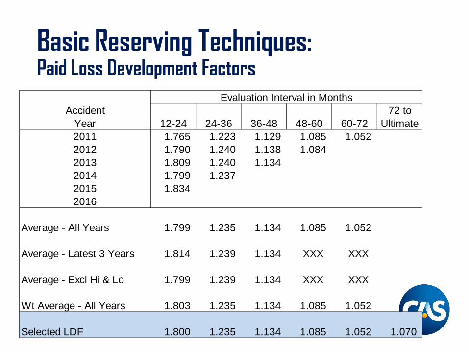
Evaluation Interval in Months
Accident 72 toYear 12-24 24-36 36-48 48-60 60-72 Ultimate2011 1.765 1.223 1.129 1.085 1.052 2012 1.790 1.240 1.138 1.084 2013 1.809 1.240 1.134 2014 1.799 1.237 2015 1.834 2016
Average - All Years 1.799 1.235 1.134 1.085 1.052
Average - Latest 3 Years 1.814 1.239 1.134 XXX XXX
Average - Excl Hi & Lo 1.799 1.239 1.134 XXX XXX
Wt Average - All Years 1.803 1.235 1.134 1.085 1.052
Selected LDF 1.800 1.235 1.134 1.085 1.052 1.070
Basic Reserving Techniques:Application of Paid LDM
Evaluation Interval in Months
72 to12-24 24-36 36-48 48-60 60-72 Ultimate
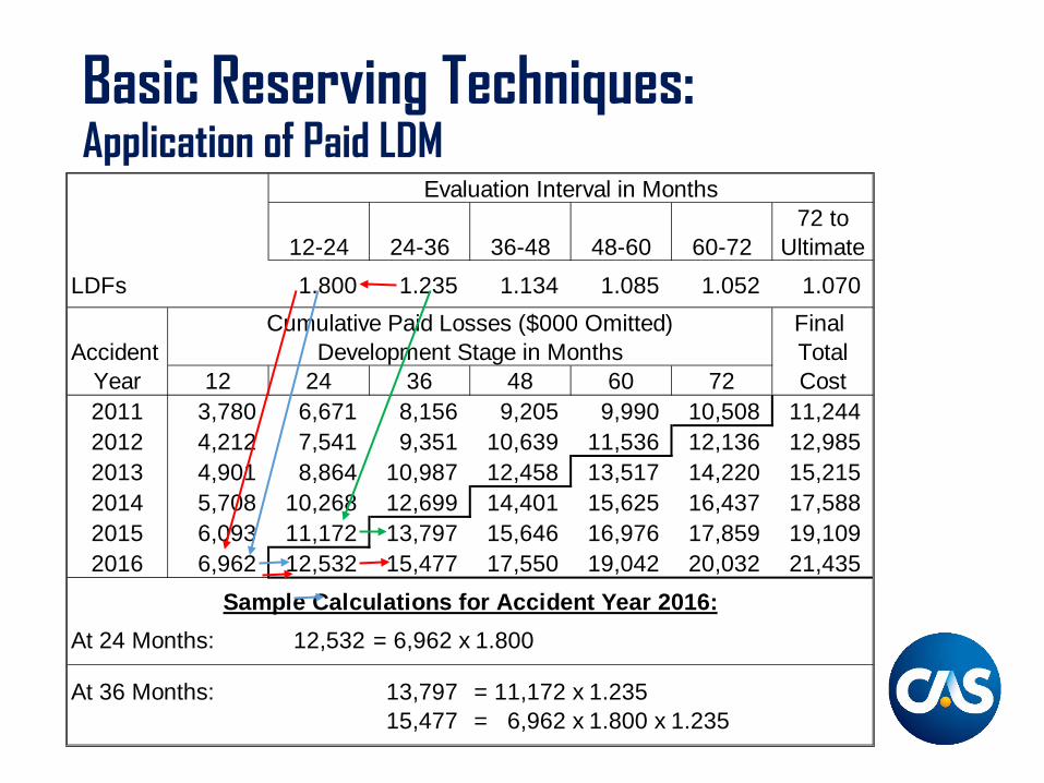
LDFs 1.800 1.235 1.134 1.085 1.052 1.070 Cumulative Paid Losses ($000 Omitted) Final
Accident Development Stage in Months TotalYear 12 24 36 48 60 72 Cost2011 3,780 6,671 8,156 9,205 9,990 10,508 11,244 2012 4,212 7,541 9,351 10,639 11,536 12,136 12,985 2013 4,901 8,864 10,987 12,458 13,517 14,220 15,215 2014 5,708 10,268 12,699 14,401 15,625 16,437 17,588 2015 6,093 11,172 13,797 15,646 16,976 17,859 19,109 2016 6,962 12,532 15,477 17,550 19,042 20,032 21,435
Sample Calculations for Accident Year 2016:
At 24 Months: 12,532 = 6,962 x 1.800
At 36 Months: 13,797 = 11,172 x 1.23515,477 = 6,962 x 1.800 x 1.235

Basic Reserving Techniques:Paid LDM Projections & Reserves
Loss Reserve Estimate @ 12/31/16 = $32.241 million
Actual Cumulative Estimated Actual EstimatedPaid Development Ultimate Paid Loss
Accident Losses Selected Factors to Losses Losses ReservesYear 12/31/16 LDFs Ultimate [(2) x (4)] 12/31/16 [(5) - (6)](1) (2) (3) (4) (5) (6) (7)
2011 10,508 1.070 1.070 11,244 10,508 736 2012 11,536 1.052 1.126 12,985 11,536 1,449 2013 12,458 1.085 1.221 15,215 12,458 2,757 2014 12,699 1.134 1.385 17,588 12,699 4,889 2015 11,172 1.235 1.710 19,109 11,172 7,937 2016 6,962 1.800 3.079 21,435 6,962 14,473
Total 65,335 97,576 65,335 32,241
Basic Reserving Techniques:Issues to Consider for Paid LDM
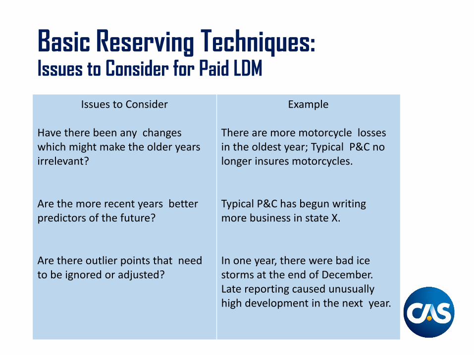
Issues to Consider
Have there been any changes which might make the older years irrelevant?
Are the more recent years better predictors of the future?
Are there outlier points that need to be ignored or adjusted?
Example
There are more motorcycle losses in the oldest year; Typical P&C no longer insures motorcycles.
Typical P&C has begun writing more business in state X.
In one year, there were bad ice storms at the end of December. Late reporting caused unusually high development in the next year.
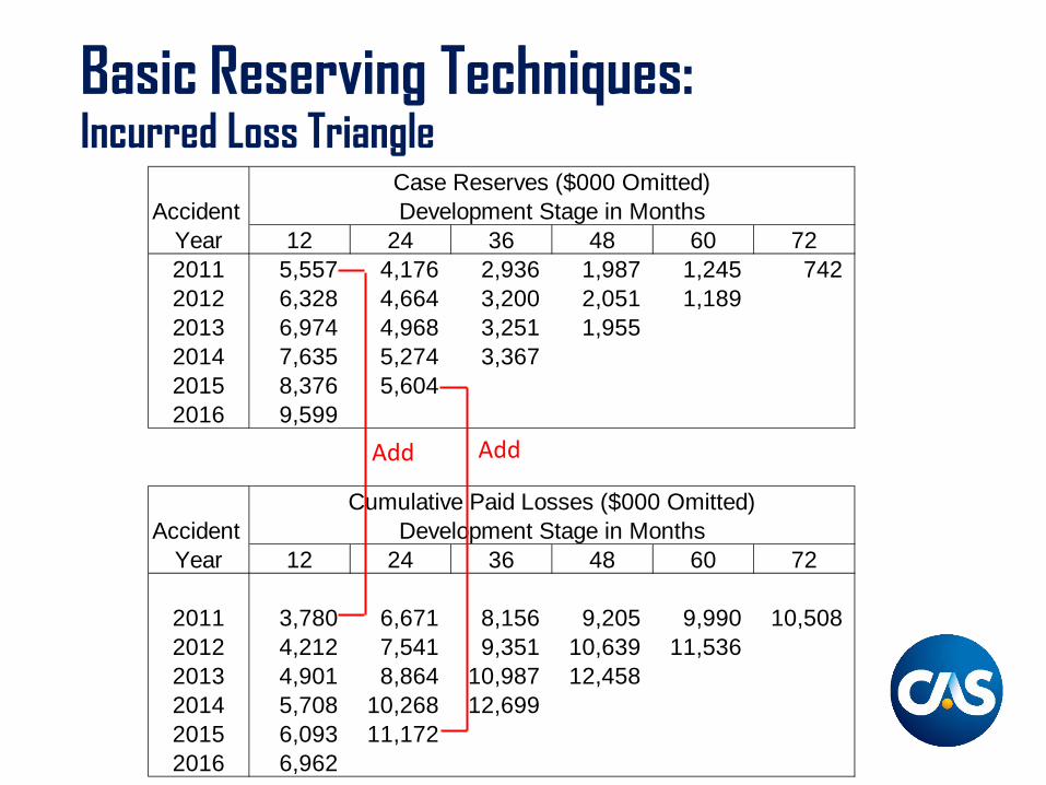
Basic Reserving Techniques:Incurred Loss Triangle
Case Reserves ($000 Omitted)Accident Development Stage in Months
Year 12 24 36 48 60 722011 5,557 4,176 2,936 1,987 1,245 742 2012 6,328 4,664 3,200 2,051 1,189 2013 6,974 4,968 3,251 1,955 2014 7,635 5,274 3,367 2015 8,376 5,604 2016 9,599
Cumulative Paid Losses ($000 Omitted)
Accident Development Stage in MonthsYear 12 24 36 48 60 72
2011 3,780 6,671 8,156 9,205 9,990 10,508 2012 4,212 7,541 9,351 10,639 11,536 2013 4,901 8,864 10,987 12,458 2014 5,708 10,268 12,699 2015 6,093 11,172 2016 6,962
AddAdd
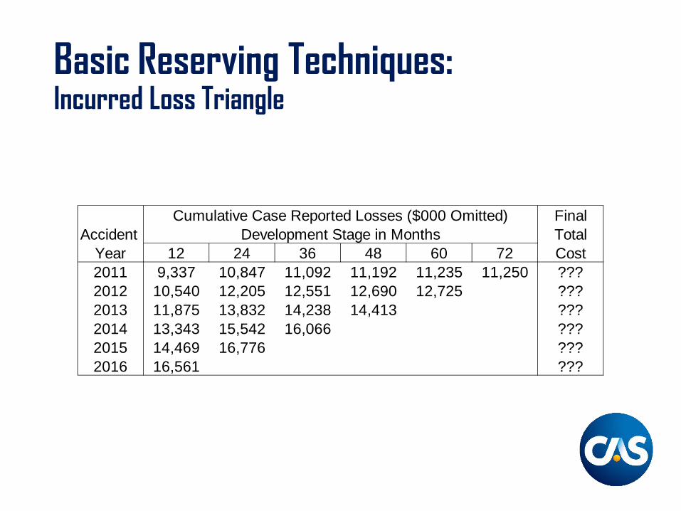
Basic Reserving Techniques:Incurred Loss Triangle
Cumulative Case Reported Losses ($000 Omitted) FinalAccident Development Stage in Months Total
Year 12 24 36 48 60 72 Cost2011 9,337 10,847 11,092 11,192 11,235 11,250 ???2012 10,540 12,205 12,551 12,690 12,725 ???2013 11,875 13,832 14,238 14,413 ???2014 13,343 15,542 16,066 ???2015 14,469 16,776 ???2016 16,561 ???
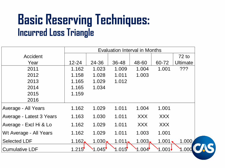
Basic Reserving Techniques:Incurred Loss Triangle
Evaluation Interval in MonthsAccident 72 to
Year 12-24 24-36 36-48 48-60 60-72 Ultimate2011 1.162 1.023 1.009 1.004 1.001 ???2012 1.158 1.028 1.011 1.003 2013 1.165 1.029 1.012 2014 1.165 1.034 2015 1.159 2016
Average - All Years 1.162 1.029 1.011 1.004 1.001 Average - Latest 3 Years 1.163 1.030 1.011 XXX XXX Average - Excl Hi & Lo 1.162 1.029 1.011 XXX XXX Wt Average - All Years 1.162 1.029 1.011 1.003 1.001 Selected LDF 1.162 1.030 1.011 1.003 1.001 1.000 Cumulative LDF 1.215 1.045 1.015 1.004 1.001 1.000

Basic Reserving Techniques:Incurred LDM Projections & Reserves
Actual Estimated Actual EstimatedReported Development Ultimate Paid Loss
Accident Losses Factors to Losses Losses ReservesYear 12/31/16 Ultimate [(2) x (3)] 12/31/16 {(4) - (5)}(1) (2) (3) (4) (5) (6)
2011 11,250 1.000 11,250 10,508 742 2012 12,725 1.001 12,738 11,536 1,202 2013 14,413 1.004 14,471 12,458 2,013 2014 16,066 1.015 16,308 12,699 3,609 2015 16,776 1.045 17,539 11,172 6,367 2016 16,561 1.215 20,119 6,962 13,157
Total 87,791 92,425 65,335 27,090
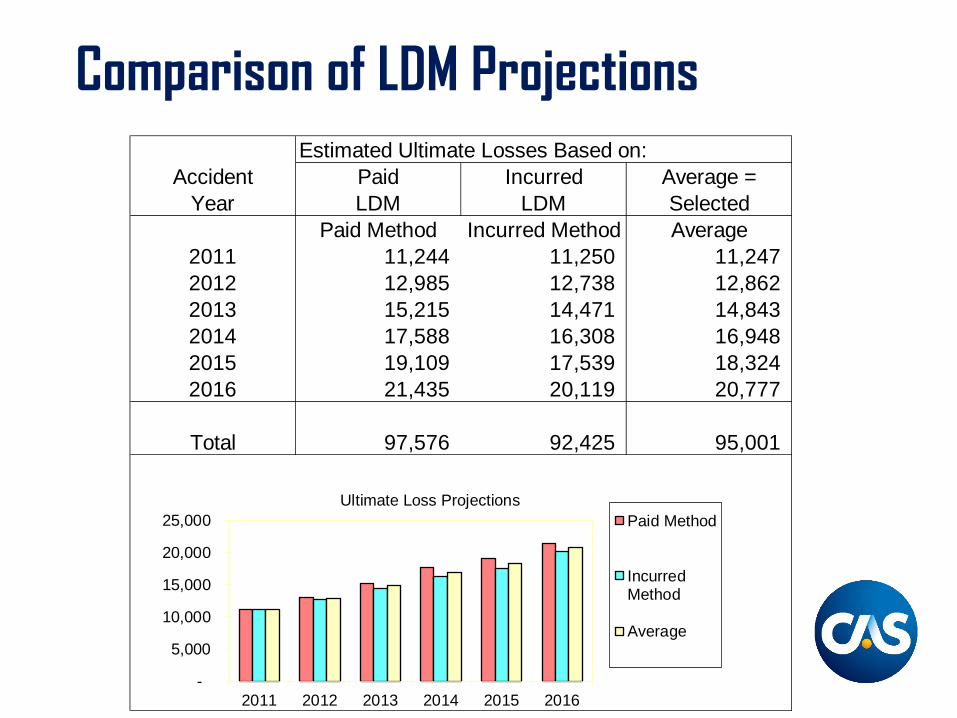
Comparison of LDM ProjectionsEstimated Ultimate Losses Based on:
Accident Paid Incurred Average =Year LDM LDM Selected
Paid Method Incurred Method Average2011 11,244 11,250 11,247 2012 12,985 12,738 12,862 2013 15,215 14,471 14,843 2014 17,588 16,308 16,948 2015 19,109 17,539 18,324 2016 21,435 20,119 20,777
Total 97,576 92,425 95,001
-
5,000
10,000
15,000
20,000
25,000
2011 2012 2013 2014 2015 2016
Ultimate Loss ProjectionsPaid Method
IncurredMethod
Average

Comparison of Loss Development Methods
Underlying Assumptions– PLDM: No changes in the payment pattern– ILDM: No changes in case reserve adequacy
Pro Con
PLDM: “Hard” data; no estimates involved
ILDM: Uses all available information
PLDM: May generate large, volatile loss development factors & take longer to develop to ultimate
ILDM: Uses case reserves, which are estimates, to develop estimates of ultimate losses
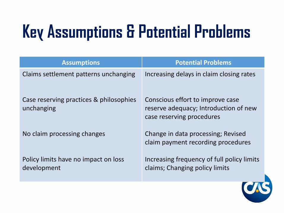
Key Assumptions & Potential Problems
Assumptions Potential Problems
Claims settlement patterns unchanging
Case reserving practices & philosophies unchanging
No claim processing changes
Policy limits have no impact on loss development
Increasing delays in claim closing rates
Conscious effort to improve case reserve adequacy; Introduction of new case reserving procedures
Change in data processing; Revised claim payment recording procedures
Increasing frequency of full policy limits claims; Changing policy limits
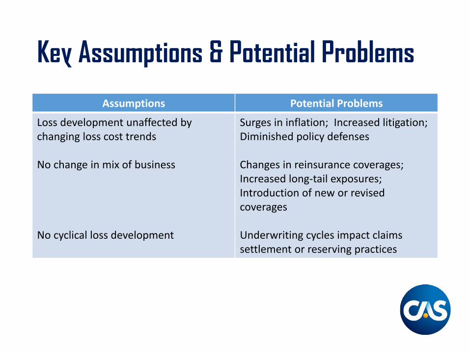
Key Assumptions & Potential Problems
Assumptions Potential Problems
Loss development unaffected by changing loss cost trends
No change in mix of business
No cyclical loss development
Surges in inflation; Increased litigation; Diminished policy defenses
Changes in reinsurance coverages; Increased long-tail exposures; Introduction of new or revised coverages
Underwriting cycles impact claims settlement or reserving practices
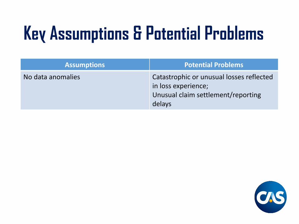
Key Assumptions & Potential Problems
Assumptions Potential Problems
No data anomalies Catastrophic or unusual losses reflected in loss experience;Unusual claim settlement/reporting delays
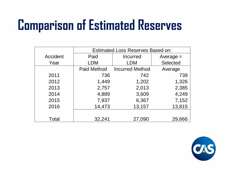
Comparison of Estimated Reserves
Estimated Loss Reserves Based on:Accident Paid Incurred Average =
Year LDM LDM SelectedPaid Method Incurred Method Average
2011 736 742 739 2012 1,449 1,202 1,326 2013 2,757 2,013 2,385 2014 4,889 3,609 4,249 2015 7,937 6,367 7,152 2016 14,473 13,157 13,815
Total 32,241 27,090 29,666
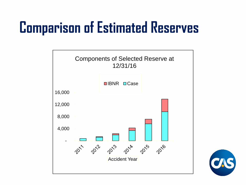
Comparison of Estimated Reserves
-
4,000
8,000
12,000
16,000
Accident Year
Components of Selected Reserve at 12/31/16
IBNR Case

Comparison of Estimated Reserves
• Which estimate is right?• Which estimate is best?• How will you know?• When will you know?
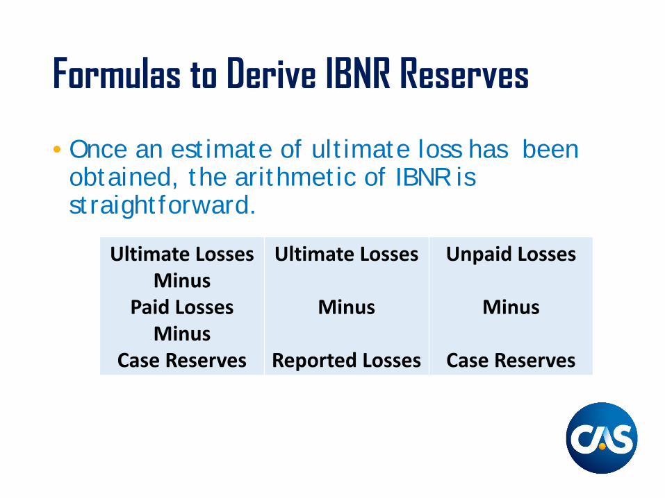
Formulas to Derive IBNR Reserves
• Once an estimate of ultimate loss has been obtained, the arithmetic of IBNR is straightforward.
Ultimate LossesMinus
Paid LossesMinus
Case Reserves
Ultimate Losses
Minus
Reported Losses
Unpaid Losses
Minus
Case Reserves
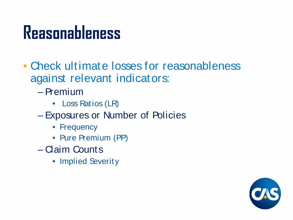
Reasonableness
• Check ultimate losses for reasonableness against relevant indicators:
– Premium• Loss Ratios (LR)
– Exposures or Number of Policies• Frequency• Pure Premium (PP)
– Claim Counts• Implied Severity
Reasonableness
• Assumptions & Methods– Document
• Notes on spreadsheets• Written report detailing assumptions
– Sensitivity analyses• Tests performed• Results of tests
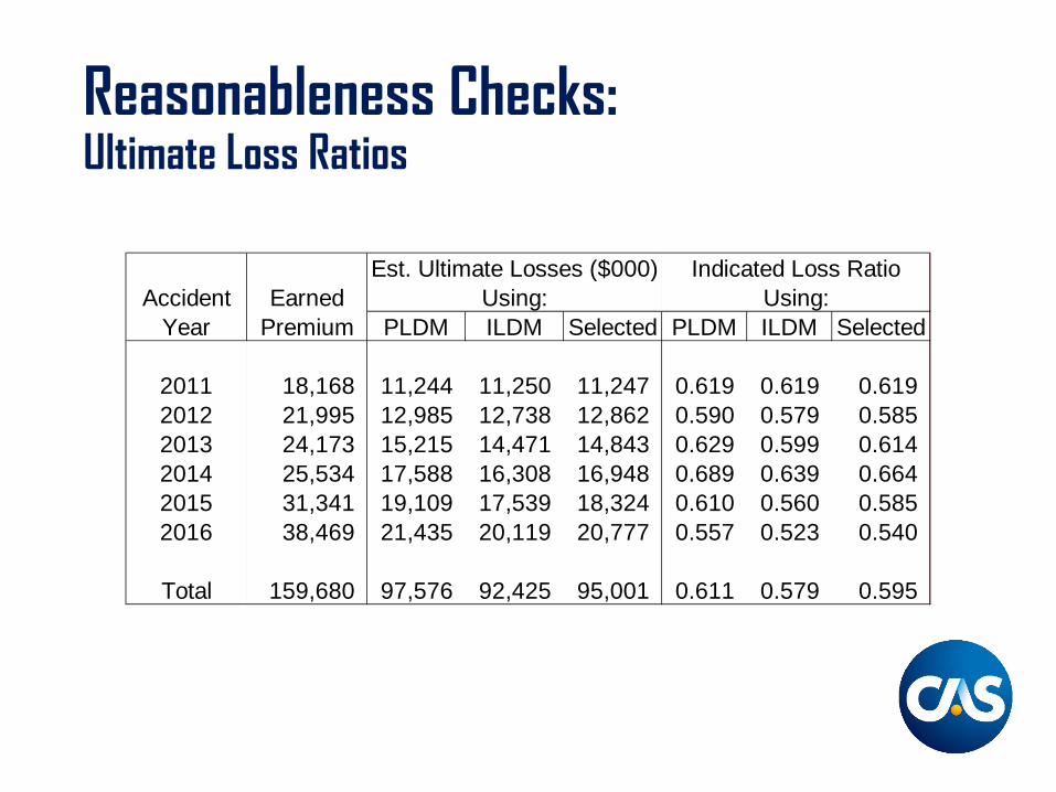
Reasonableness Checks:Ultimate Loss Ratios
Est. Ultimate Losses ($000) Indicated Loss RatioAccident Earned Using: Using:
Year Premium PLDM ILDM Selected PLDM ILDM Selected
2011 18,168 11,244 11,250 11,247 0.619 0.619 0.619 2012 21,995 12,985 12,738 12,862 0.590 0.579 0.585 2013 24,173 15,215 14,471 14,843 0.629 0.599 0.614 2014 25,534 17,588 16,308 16,948 0.689 0.639 0.664 2015 31,341 19,109 17,539 18,324 0.610 0.560 0.585 2016 38,469 21,435 20,119 20,777 0.557 0.523 0.540
Total 159,680 97,576 92,425 95,001 0.611 0.579 0.595
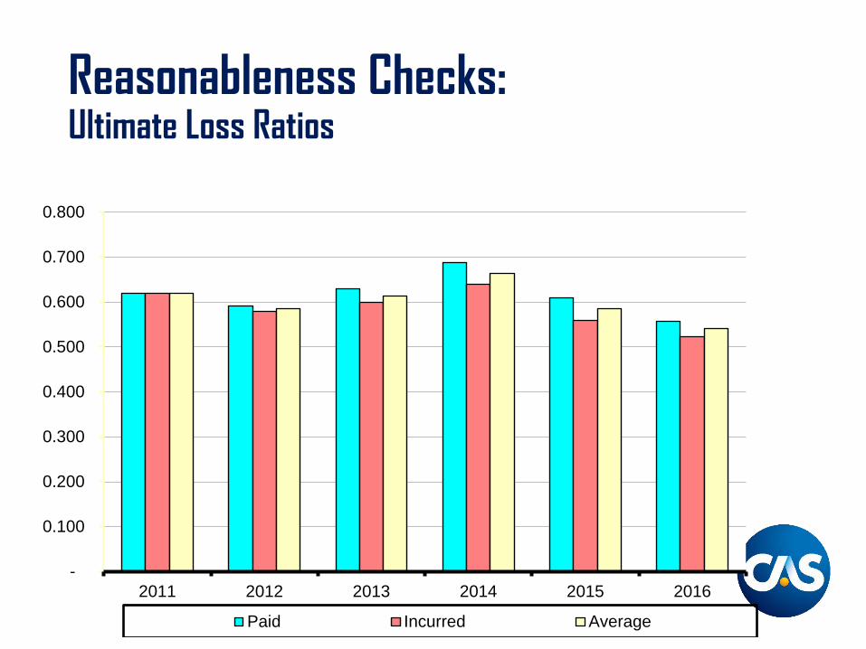
Reasonableness Checks:Ultimate Loss Ratios
-
0.100
0.200
0.300
0.400
0.500
0.600
0.700
0.800
2011 2012 2013 2014 2015 2016
Paid Incurred Average
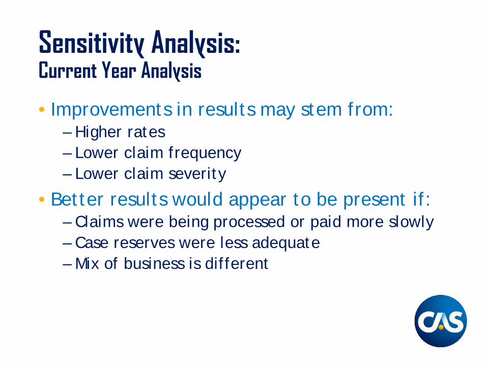
Sensitivity Analysis:Current Year Analysis
• Improvements in results may stem from:– Higher rates– Lower claim frequency– Lower claim severity
• Better results would appear to be present if:– Claims were being processed or paid more slowly– Case reserves were less adequate– Mix of business is different
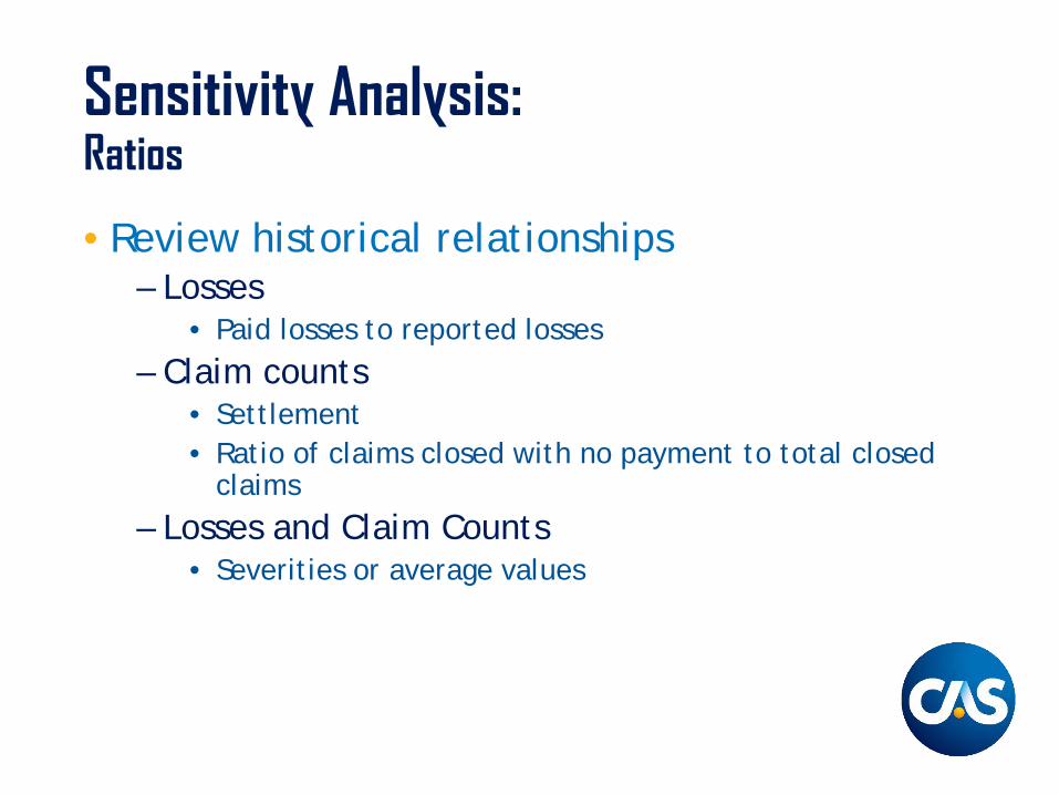
Sensitivity Analysis: Ratios
• Review historical relationships– Losses
• Paid losses to reported losses– Claim counts
• Settlement• Ratio of claims closed with no payment to total closed
claims– Losses and Claim Counts
• Severities or average values
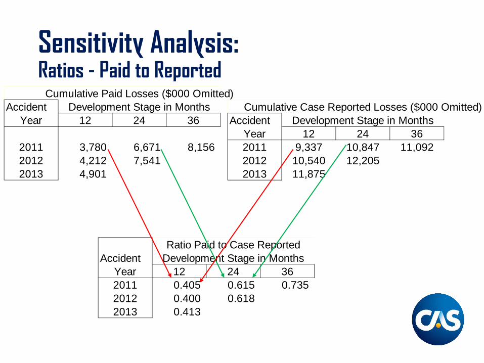
Sensitivity Analysis: Ratios - Paid to Reported
Cumulative Paid Losses ($000 Omitted)Accident Development Stage in Months
Year 12 24 36
2011 3,780 6,671 8,156 2012 4,212 7,541 2013 4,901
Cumulative Case Reported Losses ($000 Omitted)Accident Development Stage in Months
Year 12 24 362011 9,337 10,847 11,0922012 10,540 12,2052013 11,875
Ratio Paid to Case ReportedAccident Development Stage in Months
Year 12 24 362011 0.405 0.615 0.735 2012 0.400 0.618 2013 0.413
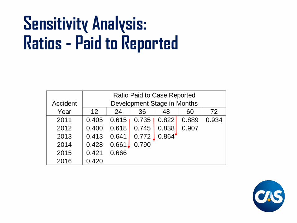
Sensitivity Analysis: Ratios - Paid to Reported
Ratio Paid to Case ReportedAccident Development Stage in Months
Year 12 24 36 48 60 722011 0.405 0.615 0.735 0.822 0.889 0.934 2012 0.400 0.618 0.745 0.838 0.907 2013 0.413 0.641 0.772 0.864 2014 0.428 0.661 0.790 2015 0.421 0.666 2016 0.420
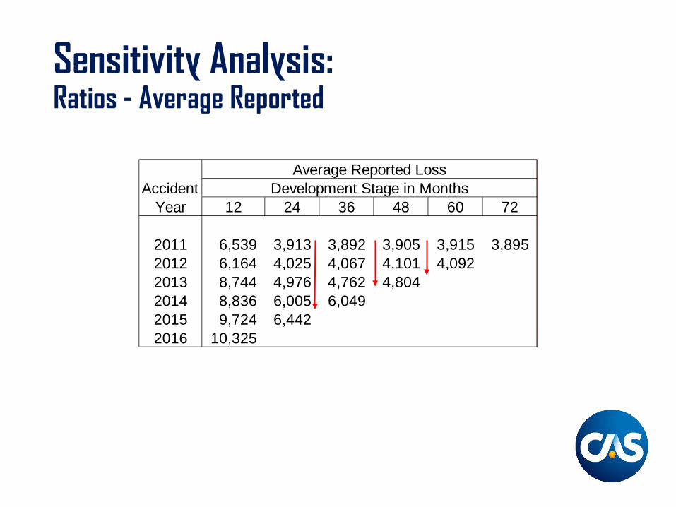
Sensitivity Analysis: Ratios - Average Reported
Average Reported Loss Accident Development Stage in Months
Year 12 24 36 48 60 72
2011 6,539 3,913 3,892 3,905 3,915 3,895 2012 6,164 4,025 4,067 4,101 4,092 2013 8,744 4,976 4,762 4,804 2014 8,836 6,005 6,049 2015 9,724 6,442 2016 10,325
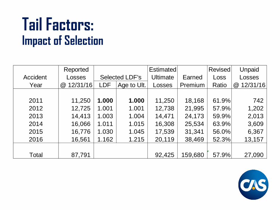
Tail Factors: Impact of Selection
Reported Estimated Revised UnpaidAccident Losses Selected LDF's Ultimate Earned Loss Losses
Year @ 12/31/16 LDF Age to Ult. Losses Premium Ratio @ 12/31/16
2011 11,250 1.000 1.000 11,250 18,168 61.9% 742 2012 12,725 1.001 1.001 12,738 21,995 57.9% 1,202 2013 14,413 1.003 1.004 14,471 24,173 59.9% 2,013 2014 16,066 1.011 1.015 16,308 25,534 63.9% 3,609 2015 16,776 1.030 1.045 17,539 31,341 56.0% 6,367 2016 16,561 1.162 1.215 20,119 38,469 52.3% 13,157
Total 87,791 92,425 159,680 57.9% 27,090

Tail Factors: Impact of Selection
Effect on Estimates Given a 2% Increase in Reported Losses Tail Factor
Reported Estimated Revised UnpaidAccident Losses Selected LDF's Ultimate Earned Loss Losses
Year @12/31/16 LDF Age to Ult. Losses Premium Ratio @12/31/16
2011 11,250 1.020 1.020 11,475 18,168 63.2% 967 2012 12,725 1.001 1.021 12,992 21,995 59.1% 1,456 2013 14,413 1.003 1.024 14,759 24,173 61.1% 2,301 2014 16,066 1.011 1.035 16,628 25,534 65.1% 3,929 2015 16,776 1.030 1.066 17,883 31,341 57.1% 6,711 2016 16,561 1.162 1.239 20,519 38,469 53.3% 13,557
Total 87,791 94,256 159,680 59.0% 28,921
Estimated Unpaid Losses Based on Original ILDM 27,090 (Without the 2% Tail Factor Increase)
Increase in Estimated Unpaid Losses Due to Increased Tail Factor 6.8%
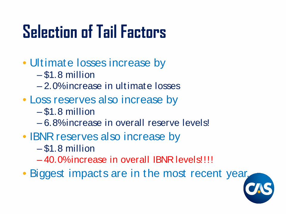
Selection of Tail Factors
• Ultimate losses increase by– $1.8 million– 2.0% increase in ultimate losses
• Loss reserves also increase by– $1.8 million– 6.8% increase in overall reserve levels!
• IBNR reserves also increase by– $1.8 million– 40.0% increase in overall IBNR levels!!!!
• Biggest impacts are in the most recent year.
Other Basic Methods
• Expected Loss– Estimating the ultimate
• Bornhuetter-Ferguson– Estimating the reserve
• Many, many others available
••••
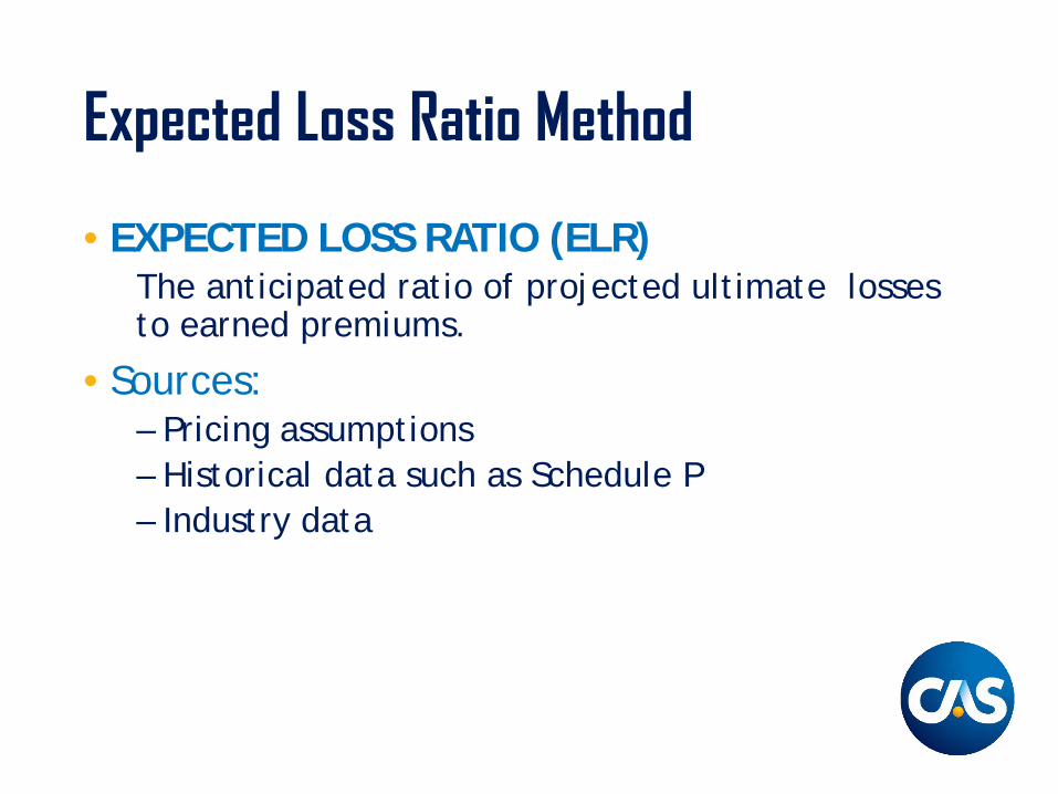
Expected Loss Ratio Method
• EXPECTED LOSS RATIO (ELR)The anticipated ratio of projected ultimate losses to earned premiums.
• Sources:– Pricing assumptions– Historical data such as Schedule P– Industry data
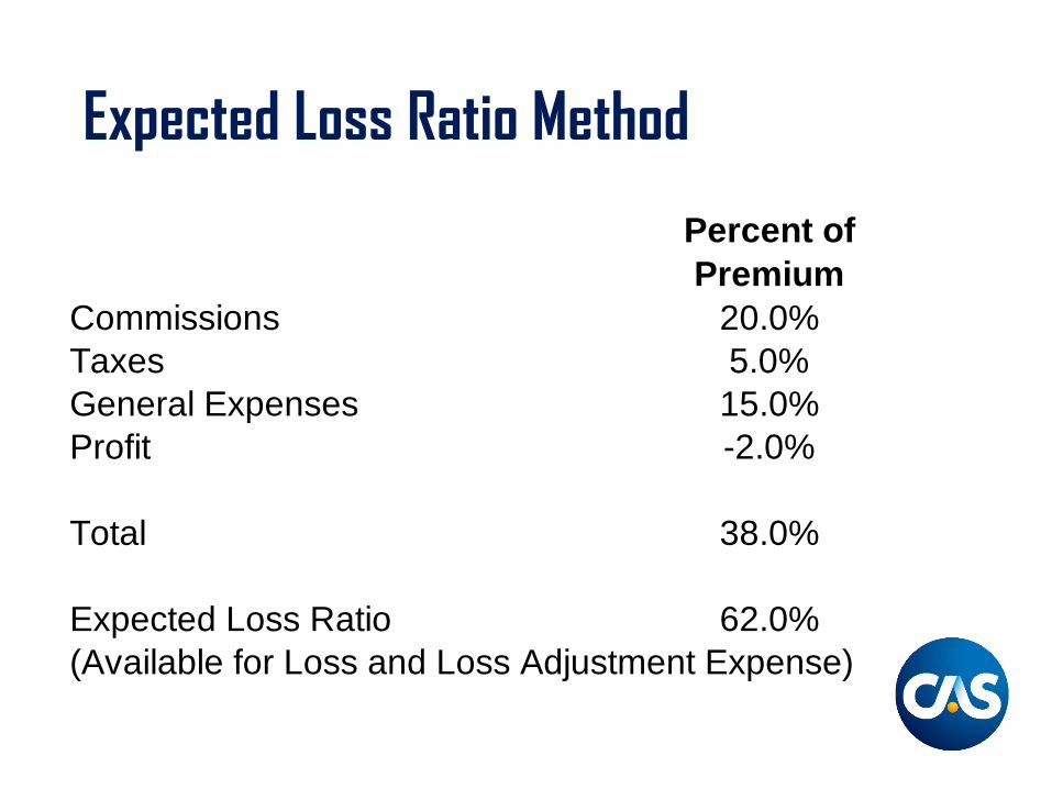
Expected Loss Ratio Method
Percent ofPremium
Commissions 20.0%Taxes 5.0%General Expenses 15.0%Profit -2.0%
Total 38.0%
Expected Loss Ratio 62.0%(Available for Loss and Loss Adjustment Expense)
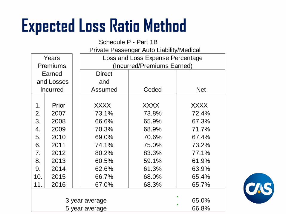
Expected Loss Ratio MethodSchedule P - Part 1B
Private Passenger Auto Liability/MedicalYears Loss and Loss Expense Percentage
Premiums (Incurred/Premiums Earned)Earned Direct
and Losses and Incurred Assumed Ceded Net
1. Prior XXXX XXXX XXXX 2. 2007 73.1% 73.8% 72.4%3. 2008 66.6% 65.9% 67.3%4. 2009 70.3% 68.9% 71.7%5. 2010 69.0% 70.6% 67.4%6. 2011 74.1% 75.0% 73.2%7. 2012 80.2% 83.3% 77.1%8. 2013 60.5% 59.1% 61.9%9. 2014 62.6% 61.3% 63.9%
10. 2015 66.7% 68.0% 65.4%11. 2016 67.0% 68.3% 65.7%
3 year average 65.0% 5 year average 66.8%
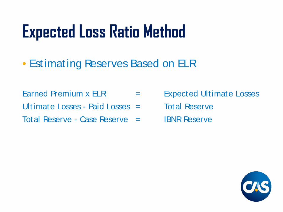
Expected Loss Ratio Method
• Estimating Reserves Based on ELR
Earned Premium x ELR = Expected Ultimate LossesUltimate Losses - Paid Losses = Total ReserveTotal Reserve - Case Reserve = IBNR Reserve
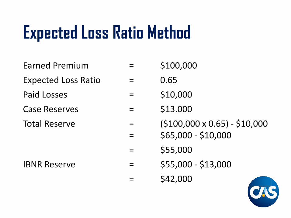
Expected Loss Ratio Method
Earned Premium = $100,000Expected Loss Ratio = 0.65Paid Losses = $10,000Case Reserves = $13.000Total Reserve =
=($100,000 x 0.65) - $10,000$65,000 - $10,000
= $55,000IBNR Reserve = $55,000 - $13,000
= $42,000
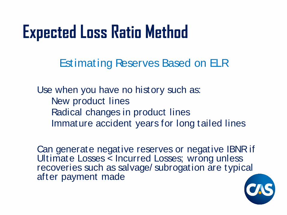
Expected Loss Ratio Method
Estimating Reserves Based on ELR
Use when you have no history such as:New product linesRadical changes in product linesImmature accident years for long tailed lines
Can generate negative reserves or negative IBNR if Ultimate Losses < Incurred Losses; wrong unless recoveries such as salvage/subrogation are typical after payment made
Bornhüetter-Ferguson Method
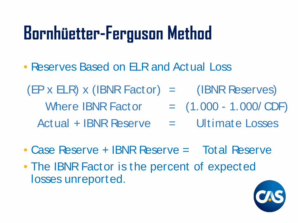
• Reserves Based on ELR and Actual Loss
• Case Reserve + IBNR Reserve = Total Reserve• The IBNR Factor is the percent of expected
losses unreported.
(EP x ELR) x (IBNR Factor) = (IBNR Reserves)Where IBNR Factor = (1.000 - 1.000/CDF)
Actual + IBNR Reserve = Ultimate Losses

Bornhüetter-Ferguson Method
+1.000 - 1.000/1.215 +1.000 - 1.000/1.015
Evaluation Interval in MonthsAccident
Year 12-24 24-36 36-482011 1.162 1.023 1.009 2012 1.158 1.028 1.011 2013 1.165 1.029 1.012 2014 1.165 1.034 2015 1.159 2016
Selected LDF 1.162 1.030 1.011 Cumulative LDF 1.215 1.045 1.015
IBNR Factor = 1.000 - 1.000/Cumulative Loss Development Factor
IBNR Factor 0.177 0.044 0.015

Bornhüetter-Ferguson MethodEvaluation Interval in Months
Accident 72 toYear 12-24 24-36 36-48 48-60 60-72 Ultimate2011 1.162 1.023 1.009 1.004 1.001 ???2012 1.158 1.028 1.011 1.003 2013 1.165 1.029 1.012 2014 1.165 1.034 2015 1.159 2016
Average - All Years 1.162 1.029 1.011 1.004 1.001 Average - Latest 3 Years 1.163 1.030 1.011 XXX XXX Average - Excl Hi & Lo 1.162 1.029 1.011 XXX XXX Wt Average - All Years 1.162 1.029 1.011 1.003 1.001 Selected LDF 1.162 1.030 1.011 1.003 1.001 1.000 Cumulative LDF 1.215 1.045 1.015 1.004 1.001 1.000
IBNR Factor = 1.000 - 1.000/Cumulative Loss Development FactorIBNR Factor 0.177 0.044 0.015 0.004 0.001 -
Bornhüetter-Ferguson Method
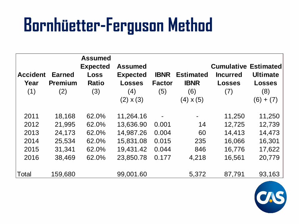
AssumedExpected Assumed Cumulative Estimated
Accident Earned Loss Expected IBNR Estimated Incurred UltimateYear Premium Ratio Losses Factor IBNR Losses Losses(1) (2) (3) (4) (5) (6) (7) (8)
(2) x (3) (4) x (5) (6) + (7)
2011 18,168 62.0% 11,264.16 - - 11,250 11,250 2012 21,995 62.0% 13,636.90 0.001 14 12,725 12,739 2013 24,173 62.0% 14,987.26 0.004 60 14,413 14,473 2014 25,534 62.0% 15,831.08 0.015 235 16,066 16,301 2015 31,341 62.0% 19,431.42 0.044 846 16,776 17,622 2016 38,469 62.0% 23,850.78 0.177 4,218 16,561 20,779
Total 159,680 99,001.60 5,372 87,791 93,163

Comparison of Methods
Expected Twice Expected Half Expected
0
5
10
15
20
25
30
35
ELR B-F LDF ELR B-F LDF ELR B-F LDF
Case Loss IBNR
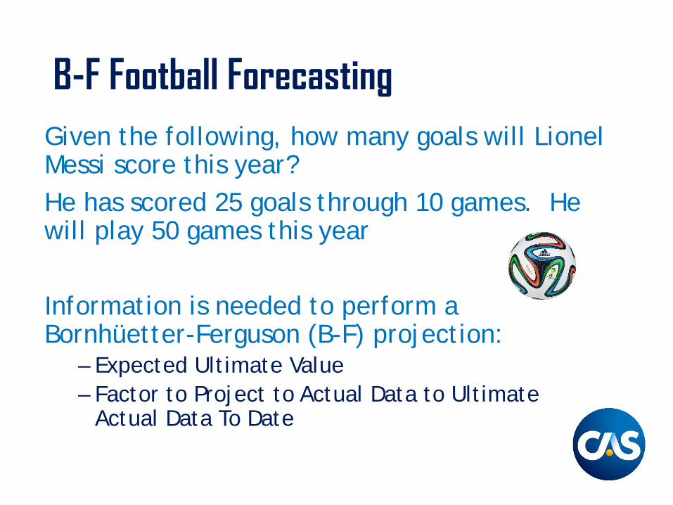
B-F Football ForecastingGiven the following, how many goals will Lionel Messi score this year?He has scored 25 goals through 10 games. He will play 50 games this year
Information is needed to perform a Bornhüetter-Ferguson (B-F) projection:
– Expected Ultimate Value– Factor to Project to Actual Data to Ultimate
Actual Data To Date

B-F Football Forecasting
Information for our example : Career averageBefore the year started, how many goals would we expect Lionel Messi to score?
Expected Ultimate Value = 50
To project season total from current statistics, multiply the current statistics by 5 since the season is 1/5 completed.
Projection Factor = 5.000He has already scored 25 goals.
Actual Goals To Date = 25
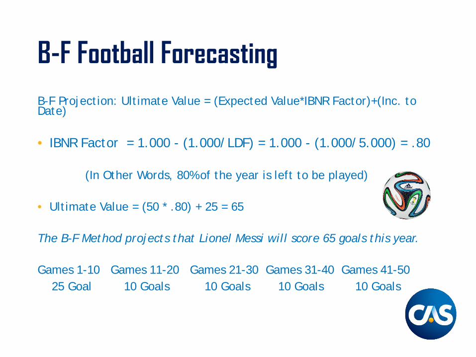
B-F Football ForecastingB-F Projection: Ultimate Value = (Expected Value*IBNR Factor)+(Inc. to Date)
• IBNR Factor = 1.000 - (1.000/LDF) = 1.000 - (1.000/5.000) = .80
(In Other Words, 80% of the year is left to be played)
• Ultimate Value = (50 * .80) + 25 = 65
The B-F Method projects that Lionel Messi will score 65 goals this year.
Games 1-10 Games 11-20 Games 21-30 Games 31-40 Games 41-5025 Goal 10 Goals 10 Goals 10 Goals 10 Goals

B-F Football ForecastingComparison of B-F with Two Other Methods
Incurred Loss Development Method
Ultimate Value = Incurred To Date * Cumulative LDF
= 25 * 5.000 = 125 Goals
Expected Loss Ratio Method
Ultimate Value = Expected Value = 50 Goals
Note: goals previously expected – 25 so far early in the season. Unless Lionel Messi is expected to slump, this method seems inappropriate.
Games 1-10 Games 11-20 Games 21-30 Games 31-40 Games 41-50
25 25 25 25 25
Games 1-10 Games 11-20 Games 21-30 Games 31-40 Games 41-50
10 10 10 10 10

Bornhüetter-Ferguson Method
ASSUMPTIONS PROBLEMSPremium is an accurate measure of exposure
Pricing Inconsistency
Expected loss ratio is predictable
Instability in accident year loss ratios
Constant reporting, case reserving and settling
Introduction of new claim systemsBacklog in processing
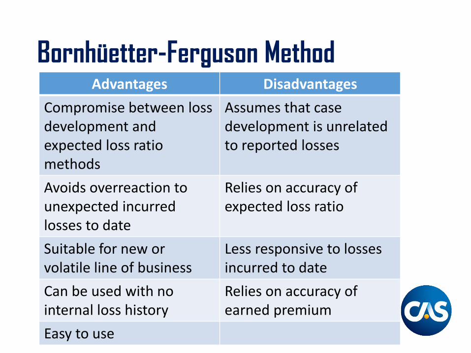
Bornhüetter-Ferguson MethodAdvantages Disadvantages
Compromise between loss development and expected loss ratio methods
Assumes that case development is unrelated to reported losses
Avoids overreaction to unexpected incurred losses to date
Relies on accuracy of expected loss ratio
Suitable for new or volatile line of business
Less responsive to losses incurred to date
Can be used with no internal loss history
Relies on accuracy of earned premium
Easy to use
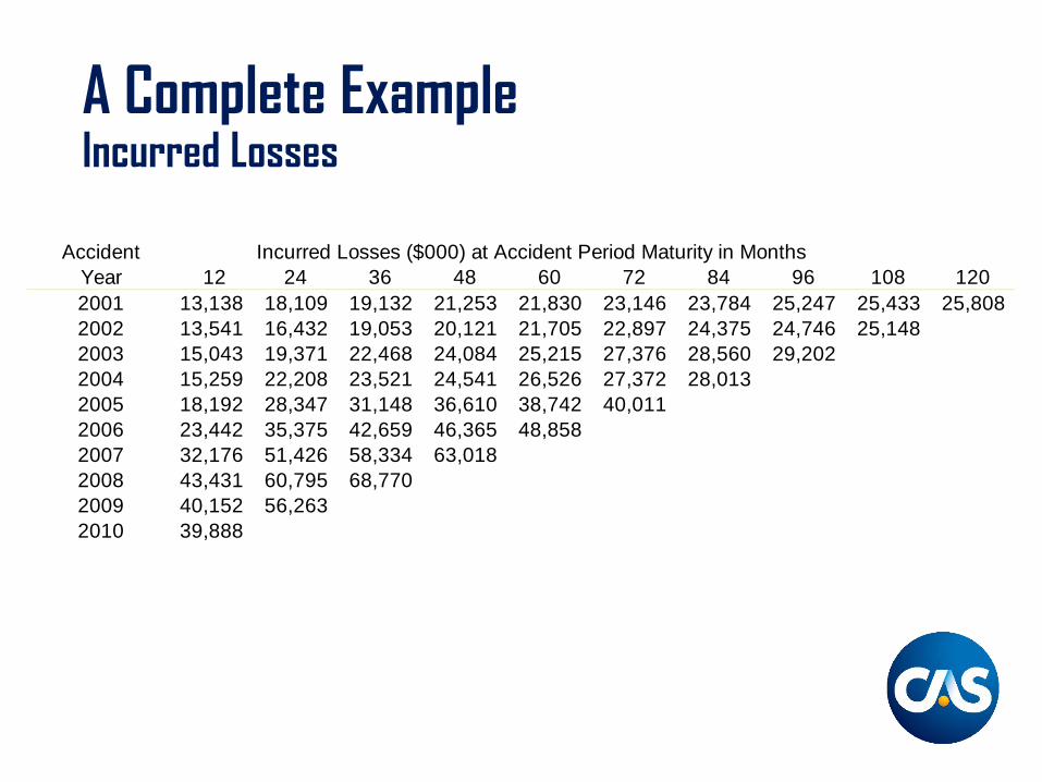
A Complete ExampleIncurred Losses
Accident Incurred Losses ($000) at Accident Period Maturity in MonthsYear 12 24 36 48 60 72 84 96 108 1202001 13,138 18,109 19,132 21,253 21,830 23,146 23,784 25,247 25,433 25,8082002 13,541 16,432 19,053 20,121 21,705 22,897 24,375 24,746 25,1482003 15,043 19,371 22,468 24,084 25,215 27,376 28,560 29,2022004 15,259 22,208 23,521 24,541 26,526 27,372 28,0132005 18,192 28,347 31,148 36,610 38,742 40,0112006 23,442 35,375 42,659 46,365 48,8582007 32,176 51,426 58,334 63,0182008 43,431 60,795 68,7702009 40,152 56,2632010 39,888
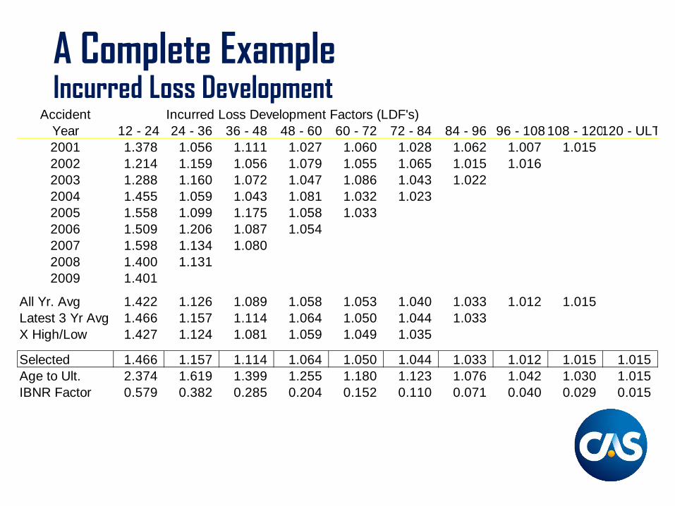
A Complete ExampleIncurred Loss Development
Accident Incurred Loss Development Factors (LDF's)Year 12 - 24 24 - 36 36 - 48 48 - 60 60 - 72 72 - 84 84 - 96 96 - 108 108 - 120120 - ULT2001 1.378 1.056 1.111 1.027 1.060 1.028 1.062 1.007 1.0152002 1.214 1.159 1.056 1.079 1.055 1.065 1.015 1.0162003 1.288 1.160 1.072 1.047 1.086 1.043 1.0222004 1.455 1.059 1.043 1.081 1.032 1.0232005 1.558 1.099 1.175 1.058 1.0332006 1.509 1.206 1.087 1.0542007 1.598 1.134 1.0802008 1.400 1.1312009 1.401
All Yr. Avg 1.422 1.126 1.089 1.058 1.053 1.040 1.033 1.012 1.015Latest 3 Yr Avg 1.466 1.157 1.114 1.064 1.050 1.044 1.033X High/Low 1.427 1.124 1.081 1.059 1.049 1.035
Selected 1.466 1.157 1.114 1.064 1.050 1.044 1.033 1.012 1.015 1.015 Age to Ult. 2.374 1.619 1.399 1.255 1.180 1.123 1.076 1.042 1.030 1.015 IBNR Factor 0.579 0.382 0.285 0.204 0.152 0.110 0.071 0.040 0.029 0.015
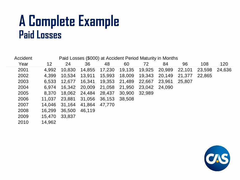
A Complete ExamplePaid Losses
Accident Paid Losses ($000) at Accident Period Maturity in MonthsYear 12 24 36 48 60 72 84 96 108 1202001 4,992 10,830 14,855 17,230 19,135 19,925 20,989 22,101 23,598 24,6362002 4,399 10,534 13,911 15,993 18,009 19,343 20,149 21,377 22,8652003 6,533 12,677 16,341 19,353 21,489 22,667 23,961 25,8072004 6,974 16,342 20,009 21,058 21,950 23,042 24,0902005 8,370 18,062 24,484 28,437 30,900 32,9892006 11,037 23,881 31,056 36,153 38,5082007 14,046 31,164 41,864 47,7702008 16,299 36,500 46,1192009 15,470 33,8372010 14,962

A Complete ExamplePaid Loss DevelopmentAccident Paid Loss Development Factors (LDF's)
Year 12 - 24 24 - 36 36 - 48 48 - 60 60 - 72 72 - 84 84 - 96 96 - 108 108 - 1202001 2.169 1.372 1.160 1.111 1.041 1.053 1.053 1.068 1.0442002 2.394 1.321 1.150 1.126 1.074 1.042 1.061 1.0702003 1.941 1.289 1.184 1.110 1.055 1.057 1.0772004 2.343 1.224 1.052 1.042 1.050 1.0462005 2.158 1.356 1.161 1.087 1.0682006 2.164 1.300 1.164 1.0652007 2.219 1.343 1.1412008 2.239 1.2642009 2.187
All Yr. Avg 2.202 1.309 1.145 1.090 1.058 1.049 1.064 1.069 1.044Latest 3 Yr Avg 2.215 1.302 1.156 1.065 1.057 1.048 1.064X High/Low 2.211 1.312 1.155 1.093 1.057 1.049
Selected 2.215 1.302 1.156 1.065 1.057 1.048 1.064 1.069 1.044 Age to Ult. 4.873 2.200 1.689 1.462 1.373 1.298 1.239 1.165 1.090 Reserve Factor 0.795 0.545 0.408 0.316 0.272 0.230 0.193 0.141 0.083
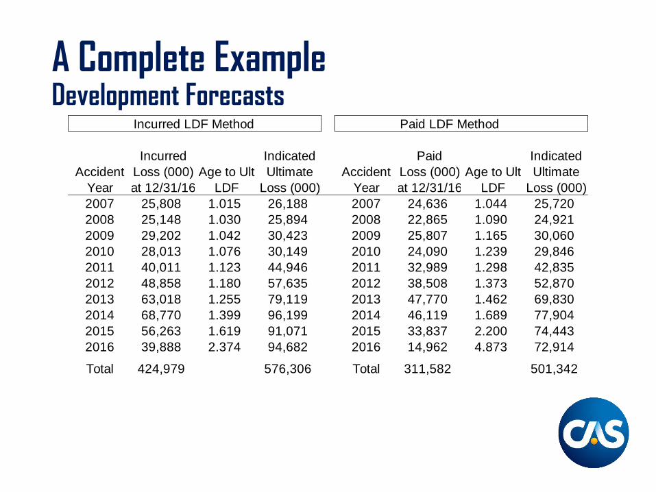
A Complete ExampleDevelopment Forecasts
Incurred LDF Method Paid LDF Method
Incurred Indicated Paid IndicatedAccident Loss (000) Age to Ult Ultimate Accident Loss (000) Age to Ult Ultimate
Year at 12/31/16 LDF Loss (000) Year at 12/31/16 LDF Loss (000)2007 25,808 1.015 26,188 2007 24,636 1.044 25,7202008 25,148 1.030 25,894 2008 22,865 1.090 24,9212009 29,202 1.042 30,423 2009 25,807 1.165 30,0602010 28,013 1.076 30,149 2010 24,090 1.239 29,8462011 40,011 1.123 44,946 2011 32,989 1.298 42,8352012 48,858 1.180 57,635 2012 38,508 1.373 52,8702013 63,018 1.255 79,119 2013 47,770 1.462 69,8302014 68,770 1.399 96,199 2014 46,119 1.689 77,9042015 56,263 1.619 91,071 2015 33,837 2.200 74,4432016 39,888 2.374 94,682 2016 14,962 4.873 72,914
Total 424,979 576,306 Total 311,582 501,342

A Complete ExampleBornhüetter-Ferguson Forecasts
Incurred BF Method Paid BF MethodIncurred Indicated Paid Indicated
Accident Earned Expected IBNR Indicated Loss (000) Ultimate Reserve Indicated Loss (000) UltimateYear Premium ELR Losses Factor IBNR at 12/31/16 Loss (000) Factor Reserve at 12/31/16 Loss (000)2007 47,975 70.0% 33,582 0.015 487 25,808 26,295 0.042 1,415 24,636 26,0512008 47,397 70.0% 33,178 0.029 956 25,148 26,104 0.083 2,737 22,865 25,6032009 46,609 70.0% 32,626 0.040 1,309 29,202 30,511 0.141 4,615 25,807 30,4232010 50,599 70.0% 35,419 0.071 2,510 28,013 30,523 0.193 6,831 24,090 30,9212011 64,637 70.0% 45,246 0.110 4,968 40,011 44,979 0.230 10,400 32,989 43,3892012 69,510 70.0% 48,657 0.152 7,410 48,858 56,268 0.272 13,218 38,508 51,7262013 86,505 70.0% 60,554 0.204 12,323 63,018 75,341 0.316 19,130 47,770 66,8992014 92,564 70.0% 64,795 0.285 18,475 68,770 87,245 0.408 26,436 46,119 72,5552015 97,248 70.0% 68,073 0.382 26,018 56,263 82,281 0.545 37,132 33,837 70,9692016 107,538 70.0% 75,276 0.579 43,563 39,888 83,452 0.795 59,830 14,962 74,792
Total 710,581 497,407 118,019 424,979 542,998 181,744 311,582 493,326

A Complete ExampleComparison of Estimates
Indicated UltimatesAccident Incurred Paid Incurred Paid Selected Selected Selected Selected
Year LDF LDF BF BF Ultimate Reserve IBNR Loss Ratio2007 26,188 25,720 26,295 26,051 26,063 1,427 256 54.3%2008 25,894 24,921 26,104 25,603 25,630 2,765 482 54.1%2009 30,423 30,060 30,511 30,423 30,354 4,547 1,152 65.1%2010 30,149 29,846 30,523 30,921 30,360 6,270 2,347 60.0%2011 44,946 42,835 44,979 43,389 44,037 11,049 4,026 68.1%2012 57,635 52,870 56,268 51,726 54,625 16,117 5,767 78.6%2013 79,119 69,830 75,341 66,899 72,797 25,027 9,779 84.2%2014 96,199 77,904 87,245 72,555 83,475 37,356 14,706 90.2%2015 91,071 74,443 82,281 70,969 79,691 45,854 23,428 81.9%2016 94,682 72,914 83,452 74,792 81,460 66,499 41,572 75.8%
Total 576,306 501,342 542,998 493,326 528,493 216,911 103,514 74.4%
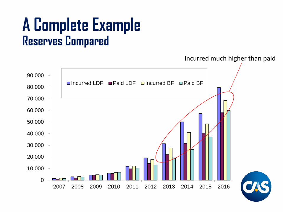
A Complete ExampleReserves Compared
0
10,000
20,000
30,000
40,000
50,000
60,000
70,000
80,000
90,000
2007 2008 2009 2010 2011 2012 2013 2014 2015 2016
Incurred LDF Paid LDF Incurred BF Paid BF
Incurred much higher than paid
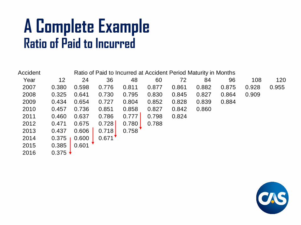
A Complete ExampleRatio of Paid to Incurred
Accident Ratio of Paid to Incurred at Accident Period Maturity in MonthsYear 12 24 36 48 60 72 84 96 108 1202007 0.380 0.598 0.776 0.811 0.877 0.861 0.882 0.875 0.928 0.9552008 0.325 0.641 0.730 0.795 0.830 0.845 0.827 0.864 0.9092009 0.434 0.654 0.727 0.804 0.852 0.828 0.839 0.8842010 0.457 0.736 0.851 0.858 0.827 0.842 0.8602011 0.460 0.637 0.786 0.777 0.798 0.8242012 0.471 0.675 0.728 0.780 0.7882013 0.437 0.606 0.718 0.7582014 0.375 0.600 0.6712015 0.385 0.6012016 0.375
Changing Conditions
• Must go beyond rote application of basic techniques to produce a meaningful reserve estimates.
• Additional considerations and diagnostic tools offer perspective in the effort to understanding risks and uncertainties.
• Communication among operating units is essential.
• Subsequent Intermediate Tracks will provide additional insights and techniques useful in addressing several of these issues.
Considerations
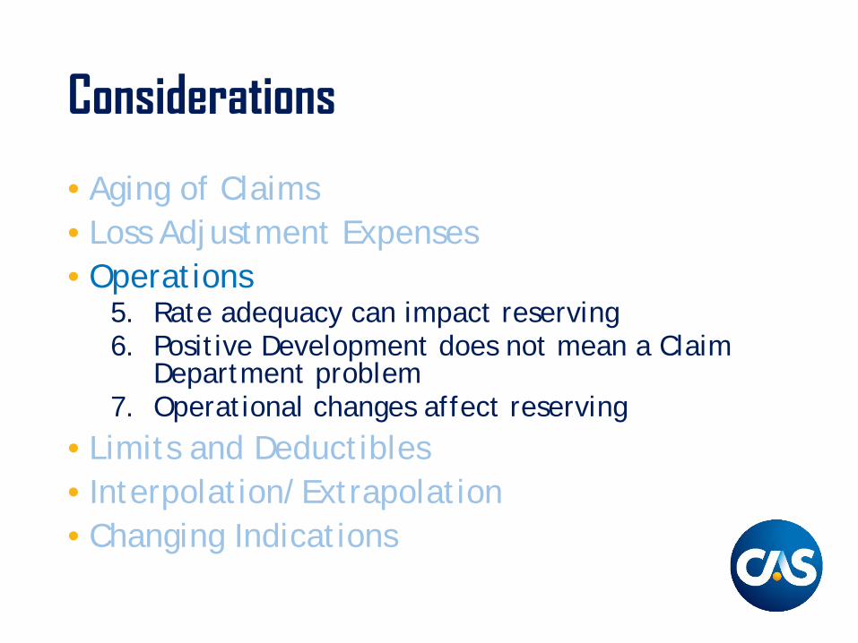
• Aging of Claims• Loss Adjustment Expenses• Operations• Limits and Deductibles• Interpolation/Extrapolation• Changing Indications
Considerations
• Aging of Claims1. Average Closed Value is not the same as Average
Open Value2. Early Reported Claims are not the same as Late
Reported Claims• Loss Adjustment Expenses• Operations• Limits and Deductibles• Interpolation/Extrapolation• Changing Indications
Consideration #1
The average value of claims closed is often a poor estimator of the ultimate average settlement value of claims still open.

Consideration #1
Accident Year 2008
Why might this frequently be true?
Cumulative Paid Number of AverageCalendar on Closed Claims Closed Claims Settlement
Date % of % of Value$ Ultimate No. Ultimate $
12-08 $50,000,000 25% 1,000 50% $50,00012-09 100,000,000 50% 1,500 75% 66,66712-10 150,000,000 75% 1,800 90% 83,333
* * * * * ** * * * * ** * * * * *
12/16 (Ult) 200,000,000 100% 2,000 100% 100,000

Consideration #1
• Claims that close early are smaller• For example in Workers Compensation:
– The cases that close quickly are usually for minor injuries, and may involve just medical-only costs.
– The cases open for a long period represent severe injuries and may include:
• Major Medical Expenses• Lifetime Pension Benefits
Consideration #2
The average costs for late reported claims may differ materially from those reported earlier.
Consideration #2
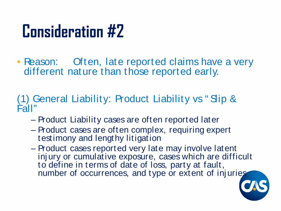
• Reason: Often, late reported claims have a very different nature than those reported early.
(1) General Liability: Product Liability vs “Slip & Fall”
– Product Liability cases are often reported later– Product cases are often complex, requiring expert
testimony and lengthy litigation– Product cases reported very late may involve latent
injury or cumulative exposure, cases which are difficult to define in terms of date of loss, party at fault, number of occurrences, and type or extent of injuries
Consideration #2
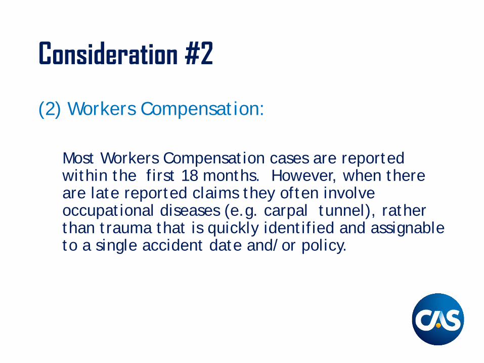
(2) Workers Compensation:
Most Workers Compensation cases are reported within the first 18 months. However, when there are late reported claims they often involve occupational diseases (e.g. carpal tunnel), rather than trauma that is quickly identified and assignable to a single accident date and/or policy.
Considerations
• Aging of Claims• Loss Adjustment Expenses
3. The ratio of Paid Expenses to Settle Individual Claims to Paid Loss increases over time
4. Segregate into Components
• Operations• Limits and Deductibles• Interpolation/Extrapolation• Changing Indications
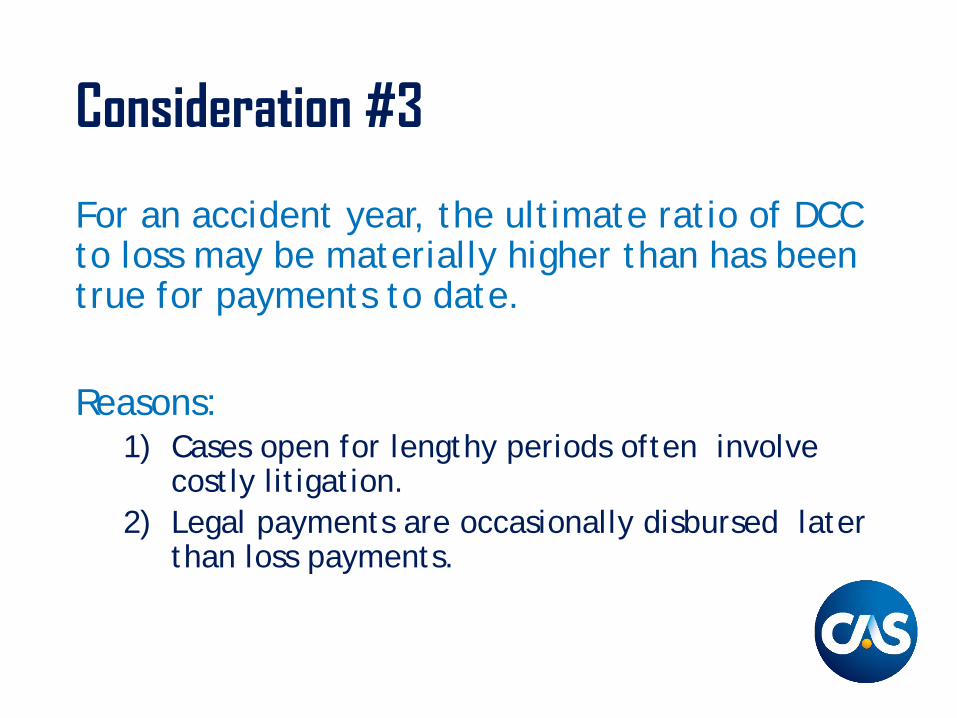
Consideration #3
For an accident year, the ultimate ratio of DCC to loss may be materially higher than has been true for payments to date.
Reasons:1) Cases open for lengthy periods often involve
costly litigation.2) Legal payments are occasionally disbursed later
than loss payments.
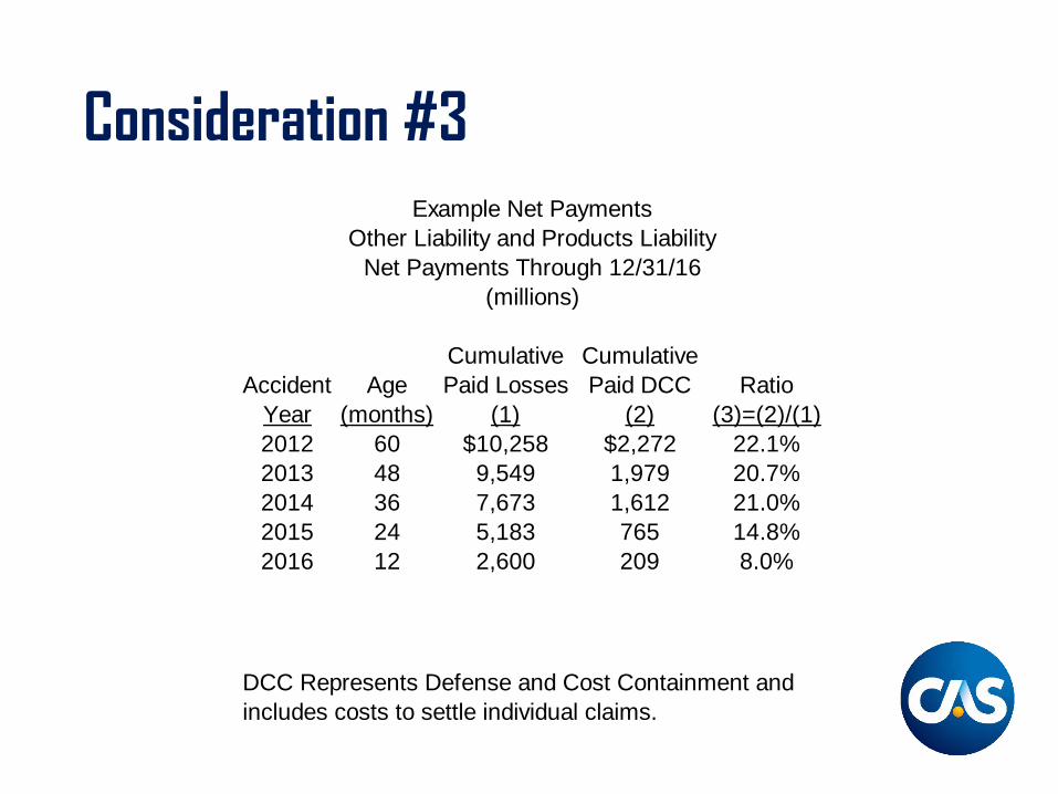
Consideration #3Example Net Payments
Other Liability and Products LiabilityNet Payments Through 12/31/16
(millions)
Cumulative CumulativeAccident Age Paid Losses Paid DCC Ratio
Year (months) (1) (2) (3)=(2)/(1)2012 60 $10,258 $2,272 22.1%2013 48 9,549 1,979 20.7%2014 36 7,673 1,612 21.0%2015 24 5,183 765 14.8%2016 12 2,600 209 8.0%
DCC Represents Defense and Cost Containment and includes costs to settle individual claims.
Consideration #3
• This pattern by company can be influenced by many factors, such as the mode of payment of legal bills, which may vary by company between:
– Interim Case Billing– End of Case Billing
• Other influences can include:– Geographical Differences– Use of Staff Counsel vs. Outside Counsel– Classes of Business– Primary vs. Excess Contracts
Consideration #4
• Where claim defense costs are volatile, it may be useful to split it into components such as:
– Attorney Fees (External or Internal)– Other Legal– Expert Witnesses– Medical Audits/Reviews
Consideration #4
Reasons:1. Legal expense are typically the fastest growing
component of DCC, with a growth rate exceeding trends in loss costs.
2. Many companies have attempted cost savings steps such as:– Use of staff counsel, rather than independent
attorneys, in some situations– Use of companies which audit legal bills– More vigorous defense (which may slow payment
patterns on loss side)– Initiating contact with the claimant sooner
Considerations
• Aging of Claims• Loss Adjustment Expenses• Operations
5. Rate adequacy can impact reserving6. Positive Development does not mean a Claim
Department problem7. Operational changes affect reserving
• Limits and Deductibles• Interpolation/Extrapolation• Changing Indications
Consideration #5
Expected Loss Ratios based on prior years’ experience, used in reserving, must be adjusted for any material changes in rate adequacy.

Consideration #5
If adjustments are not made, severe distortions can result:
Reserves Ratio of ReservesAccident Earned Paid 2013 Loss Using 2013 Actual Rates to Actual Using Actual
Year Premium Losses Ratio Loss Ratio Adequate Rates Loss Ratio Loss Ratio(1) (2) (3) (4) (5)=(2)x(4)-(3) (6) (7)=(4) / (6) (8)=(2)x(7)-(3)
2014 10,000 5,000 50% 0 1.0 50% 02015 9,000 2,700 50% 1,800 0.9 56% 2,3002016 8,000 800 50% 3,200 0.8 63% 4,200Total 8,500 5,000 6,500
Error = $1,500
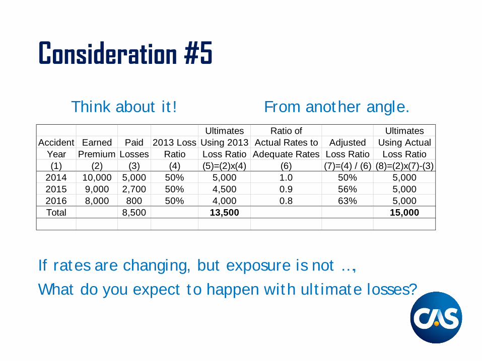
Consideration #5
Think about it! From another angle.
If rates are changing, but exposure is not …,What do you expect to happen with ultimate losses?
Ultimates Ratio of UltimatesAccident Earned Paid 2013 Loss Using 2013 Actual Rates to Adjusted Using Actual
Year Premium Losses Ratio Loss Ratio Adequate Rates Loss Ratio Loss Ratio(1) (2) (3) (4) (5)=(2)x(4) (6) (7)=(4) / (6) (8)=(2)x(7)-(3)
2014 10,000 5,000 50% 5,000 1.0 50% 5,0002015 9,000 2,700 50% 4,500 0.9 56% 5,0002016 8,000 800 50% 4,000 0.8 63% 5,000Total 8,500 13,500 15,000
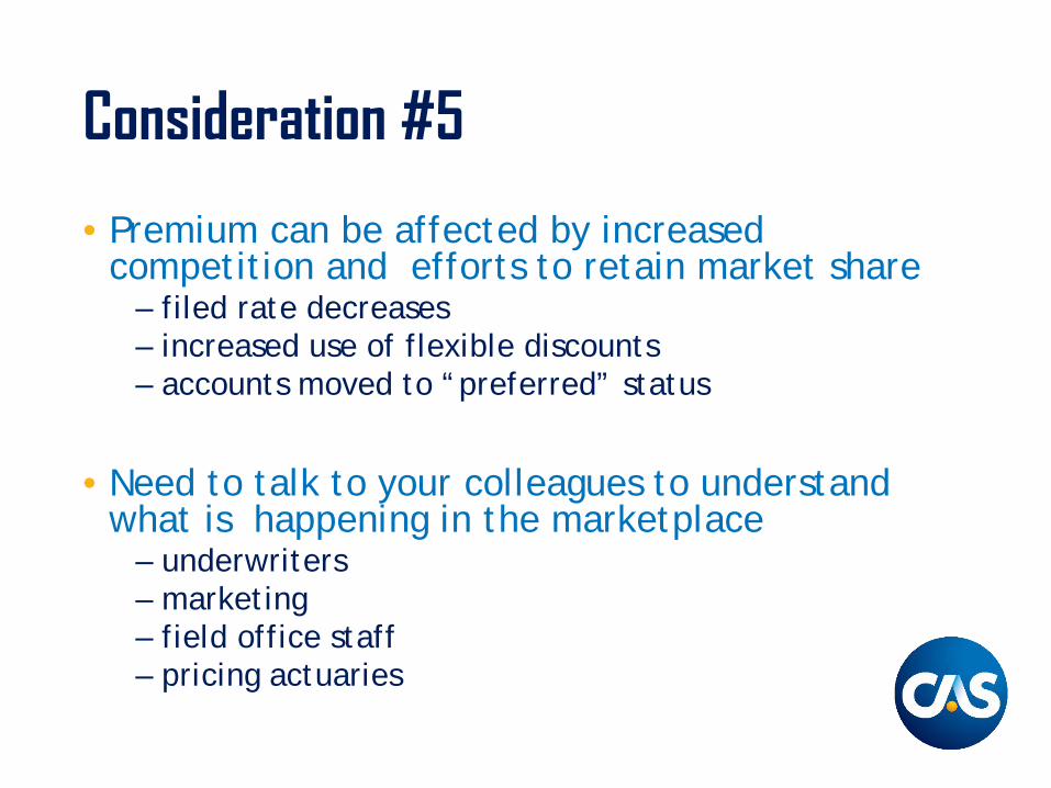
Consideration #5
• Premium can be affected by increased competition and efforts to retain market share
– filed rate decreases– increased use of flexible discounts– accounts moved to “preferred” status
• Need to talk to your colleagues to understand what is happening in the marketplace
– underwriters– marketing– field office staff– pricing actuaries
Consideration #6
Upward case development does not necessarily demonstrate something “needs fixing” in the Claims Department.
Consideration #6
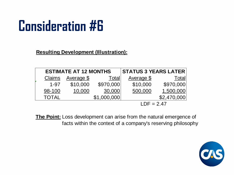
Resulting Development (Illustration):
ESTIMATE AT 12 MONTHS STATUS 3 YEARS LATERClaims Average $ Total Average $ Total
1-97 $10,000 $970,000 $10,000 $970,00098-100 10,000 30,000 500,000 1,500,000TOTAL $1,000,000 $2,470,000
LDF = 2.47
The Point: Loss development can arise from the natural emergence offacts within the context of a company's reserving philosophy
Consideration #7
Internal company changes can dramatically affect patterns in reserving data, and distort the result of basic reserving methodologies.
Consideration #7
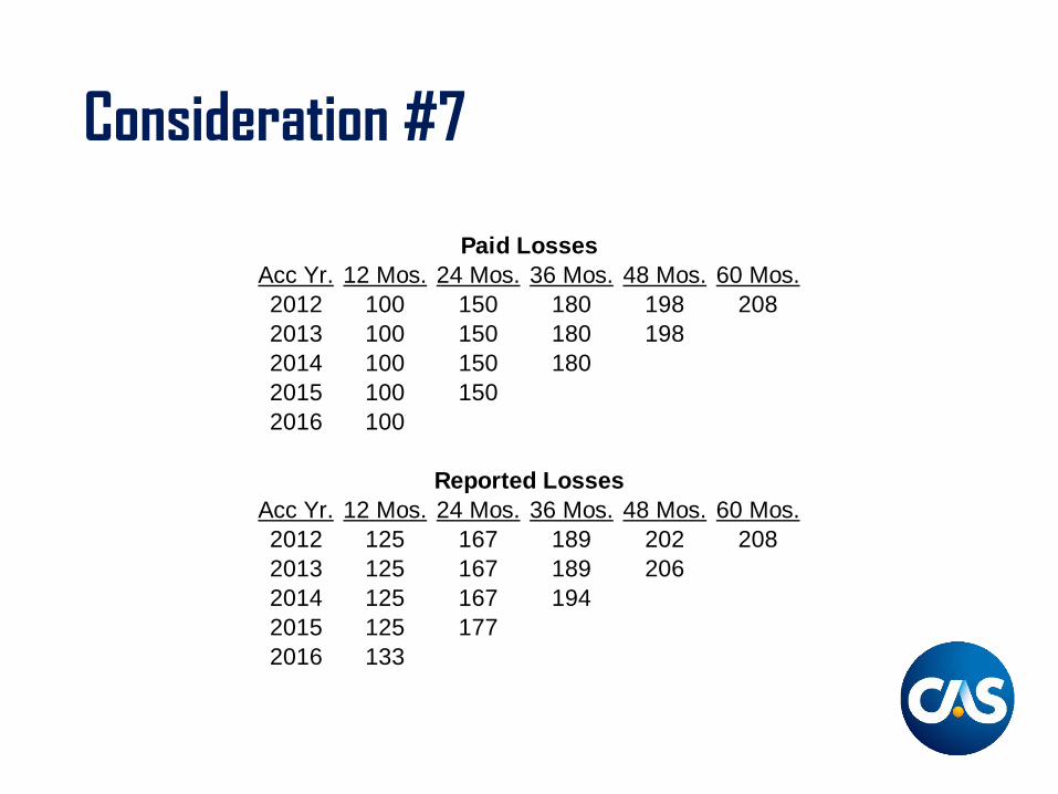
Paid LossesAcc Yr. 12 Mos. 24 Mos. 36 Mos. 48 Mos. 60 Mos.2012 100 150 180 198 2082013 100 150 180 1982014 100 150 1802015 100 1502016 100
Reported LossesAcc Yr. 12 Mos. 24 Mos. 36 Mos. 48 Mos. 60 Mos.2012 125 167 189 202 2082013 125 167 189 2062014 125 167 1942015 125 1772016 133
Consideration #7
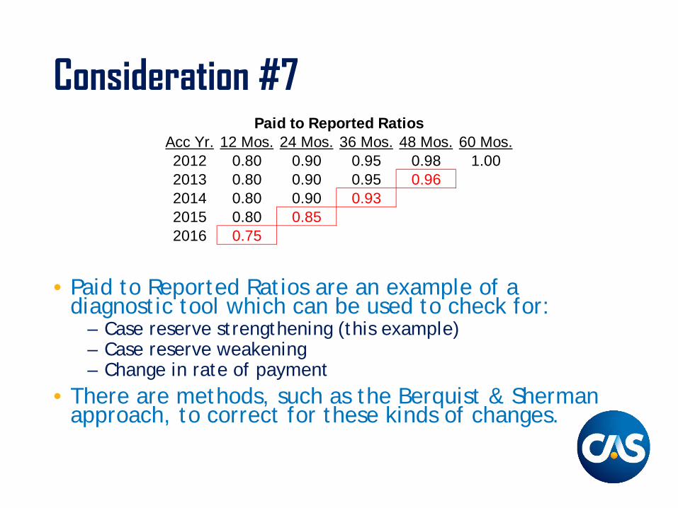
• Paid to Reported Ratios are an example of a diagnostic tool which can be used to check for:
– Case reserve strengthening (this example)– Case reserve weakening– Change in rate of payment
• There are methods, such as the Berquist & Sherman approach, to correct for these kinds of changes.
Paid to Reported RatiosAcc Yr. 12 Mos. 24 Mos. 36 Mos. 48 Mos. 60 Mos.2012 0.80 0.90 0.95 0.98 1.002013 0.80 0.90 0.95 0.962014 0.80 0.90 0.932015 0.80 0.852016 0.75
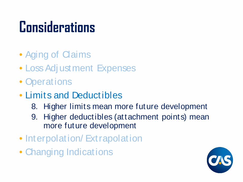
Considerations
• Aging of Claims• Loss Adjustment Expenses• Operations• Limits and Deductibles
8. Higher limits mean more future development9. Higher deductibles (attachment points) mean
more future development
• Interpolation/Extrapolation• Changing Indications
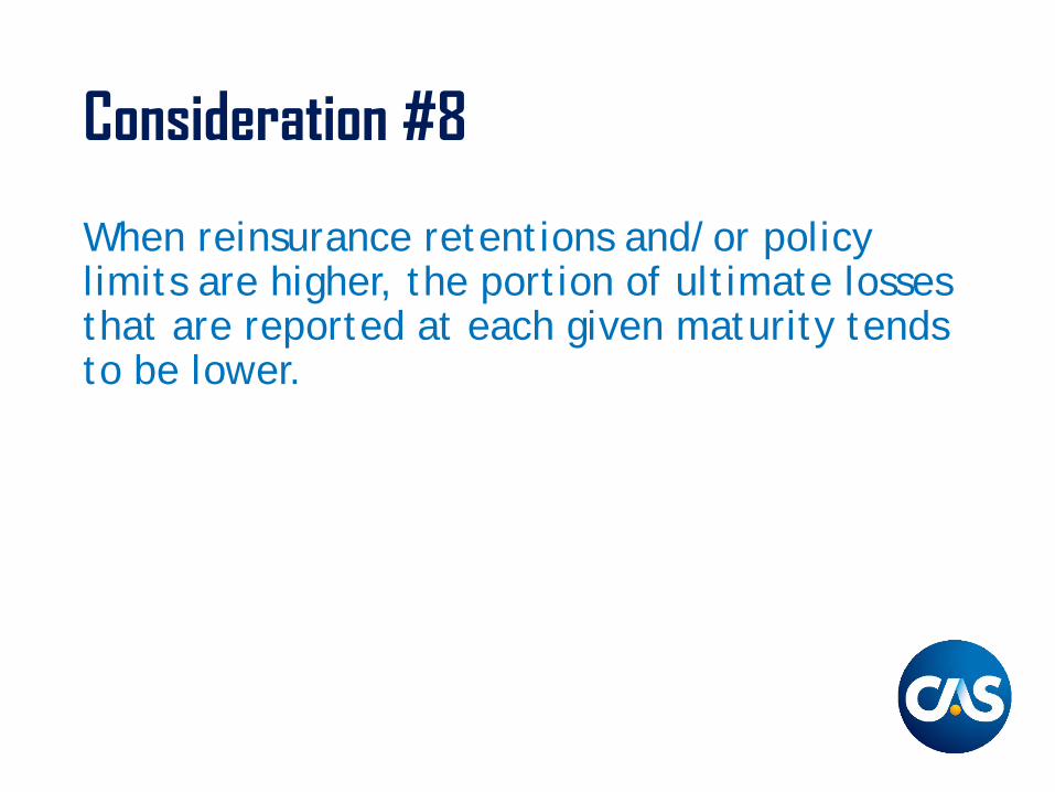
Consideration #8
When reinsurance retentions and/or policy limits are higher, the portion of ultimate losses that are reported at each given maturity tends to be lower.
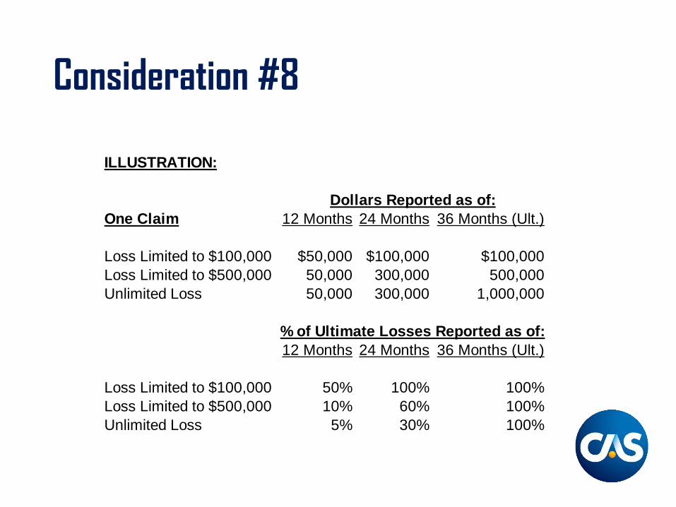
Consideration #8
ILLUSTRATION:
Dollars Reported as of:One Claim 12 Months 24 Months 36 Months (Ult.)
Loss Limited to $100,000 $50,000 $100,000 $100,000Loss Limited to $500,000 50,000 300,000 500,000Unlimited Loss 50,000 300,000 1,000,000
% of Ultimate Losses Reported as of:12 Months 24 Months 36 Months (Ult.)
Loss Limited to $100,000 50% 100% 100%Loss Limited to $500,000 10% 60% 100%Unlimited Loss 5% 30% 100%
Consideration #9
When attachment points are higher for reinsurance, excess, umbrella or self-insured coverages, then the percentage of ultimate dollars that is reported at each given maturity tends to be lower.
Consideration #9
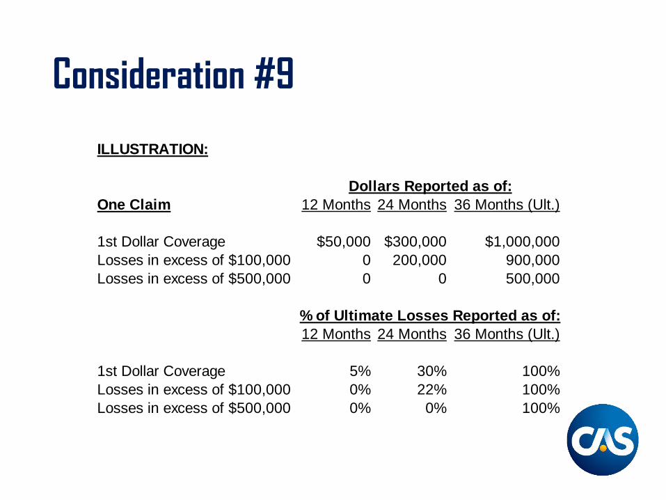
ILLUSTRATION:
Dollars Reported as of:One Claim 12 Months 24 Months 36 Months (Ult.)
1st Dollar Coverage $50,000 $300,000 $1,000,000Losses in excess of $100,000 0 200,000 900,000Losses in excess of $500,000 0 0 500,000
% of Ultimate Losses Reported as of:12 Months 24 Months 36 Months (Ult.)
1st Dollar Coverage 5% 30% 100%Losses in excess of $100,000 0% 22% 100%Losses in excess of $500,000 0% 0% 100%
Considerations
• Aging of Claims• Loss Adjustment Expenses• Operations• Limits and Deductibles• Interpolation/Extrapolation
10.Incomplete accident years can be deceiving11.Tail development is important
• Changing Indications
Consideration #10
Estimating ultimate losses for an incomplete accident year requires special adjustments.
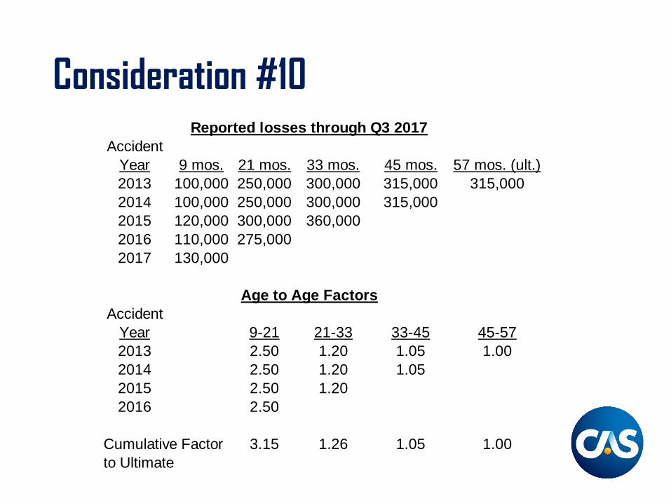
Consideration #10Reported losses through Q3 2017
AccidentYear 9 mos. 21 mos. 33 mos. 45 mos. 57 mos. (ult.)2013 100,000 250,000 300,000 315,000 315,0002014 100,000 250,000 300,000 315,0002015 120,000 300,000 360,0002016 110,000 275,0002017 130,000
Age to Age FactorsAccident
Year 9-21 21-33 33-45 45-572013 2.50 1.20 1.05 1.002014 2.50 1.20 1.052015 2.50 1.202016 2.50
Cumulative Factor 3.15 1.26 1.05 1.00to Ultimate
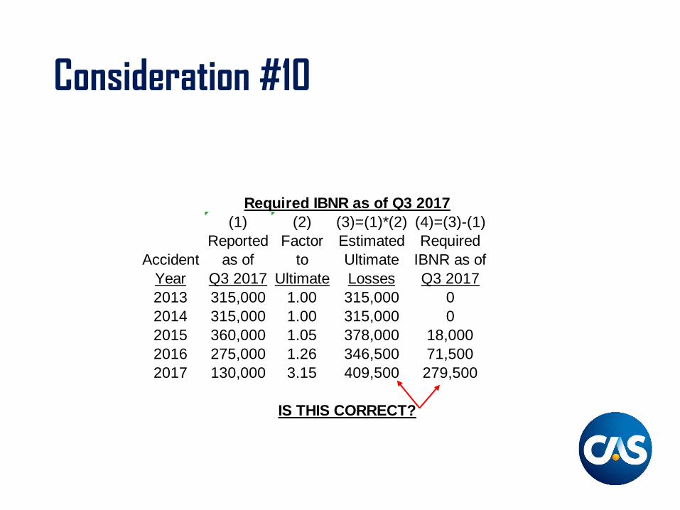
Consideration #10
Required IBNR as of Q3 2017(1) (2) (3)=(1)*(2) (4)=(3)-(1)
Reported Factor Estimated RequiredAccident as of to Ultimate IBNR as of
Year Q3 2017 Ultimate Losses Q3 20172013 315,000 1.00 315,000 02014 315,000 1.00 315,000 02015 360,000 1.05 378,000 18,0002016 275,000 1.26 346,500 71,5002017 130,000 3.15 409,500 279,500
IS THIS CORRECT?
Consideration #10
Estimating ultimate losses for an incomplete accident year requires special adjustments.
The latest year needs to be reduced by .75 for the incomplete policy period. Future claims for the final quarter need to be excluded.
Consideration #11
“Tail Development” can have a dramatic effect on reserve needs.
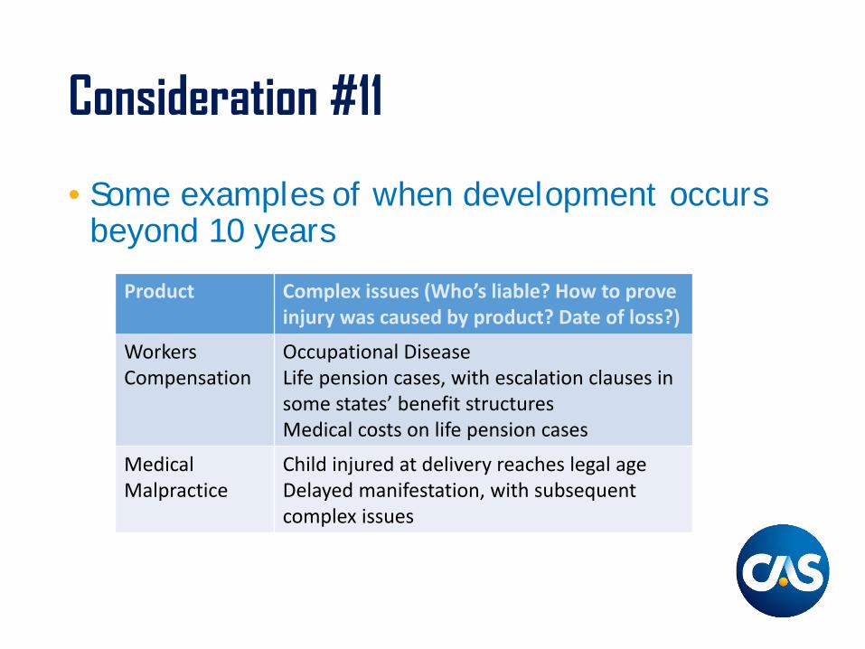
Consideration #11
• Some examples of when development occurs beyond 10 years
Product Complex issues (Who’s liable? How to prove injury was caused by product? Date of loss?)
Workers Compensation
Occupational DiseaseLife pension cases, with escalation clauses in some states’ benefit structuresMedical costs on life pension cases
MedicalMalpractice
Child injured at delivery reaches legal ageDelayed manifestation, with subsequent complex issues
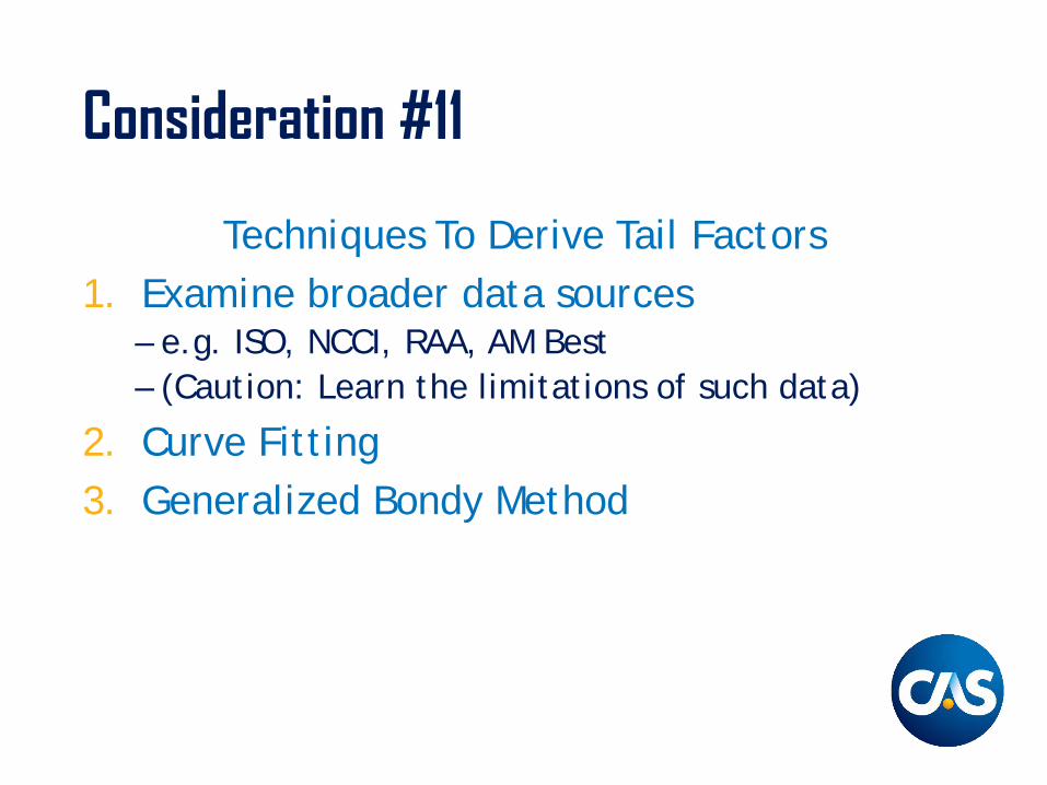
Consideration #11
Techniques To Derive Tail Factors1. Examine broader data sources
– e.g. ISO, NCCI, RAA, AM Best– (Caution: Learn the limitations of such data)
2. Curve Fitting3. Generalized Bondy Method
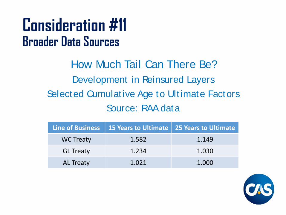
Consideration #11Broader Data Sources
How Much Tail Can There Be?Development in Reinsured Layers
Selected Cumulative Age to Ultimate FactorsSource: RAA data
Line of Business 15 Years to Ultimate 25 Years to Ultimate
WC Treaty 1.582 1.149
GL Treaty 1.234 1.030
AL Treaty 1.021 1.000
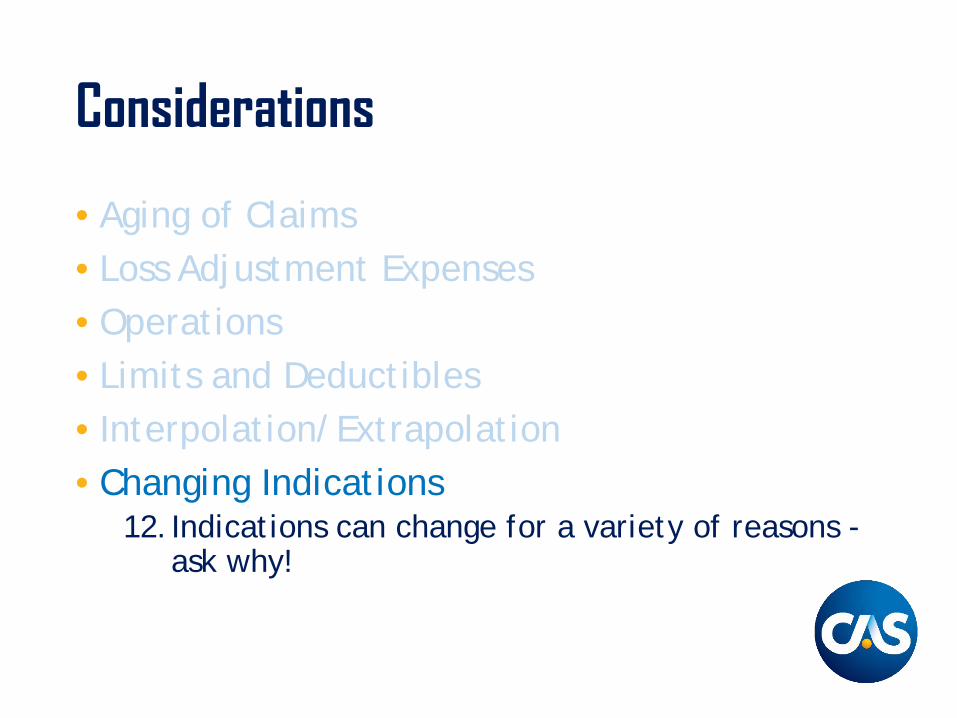
Considerations
• Aging of Claims• Loss Adjustment Expenses• Operations• Limits and Deductibles• Interpolation/Extrapolation• Changing Indications
12.Indications can change for a variety of reasons -ask why!
Consideration #12
• Why do indications change?– Actual losses emergence differs from expected.– Assumptions and/or methods change.
Consideration #12
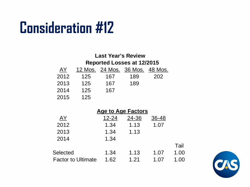
AY 12 Mos. 24 Mos. 36 Mos. 48 Mos.2012 125 167 189 2022013 125 167 1892014 125 1672015 125
Age to Age FactorsAY 12-24 24-36 36-48
2012 1.34 1.13 1.072013 1.34 1.132014 1.34
TailSelected 1.34 1.13 1.07 1.00Factor to Ultimate 1.62 1.21 1.07 1.00
Reported Losses at 12/2015Last Year's Review

Consideration #12
Easy, Right?
Reported FactorLosses to Estimated
AY at 12/2015 Ultimate Ultimate2012 202 1.00 2022013 189 1.07 2022014 167 1.21 2022015 125 1.62 202
Consideration #12
12 months later the actuary returns:
“Bad news, boss...We have to take a big hit to cover deterioration in the prior years.”
Will this be a pleasant discussion? What happened????
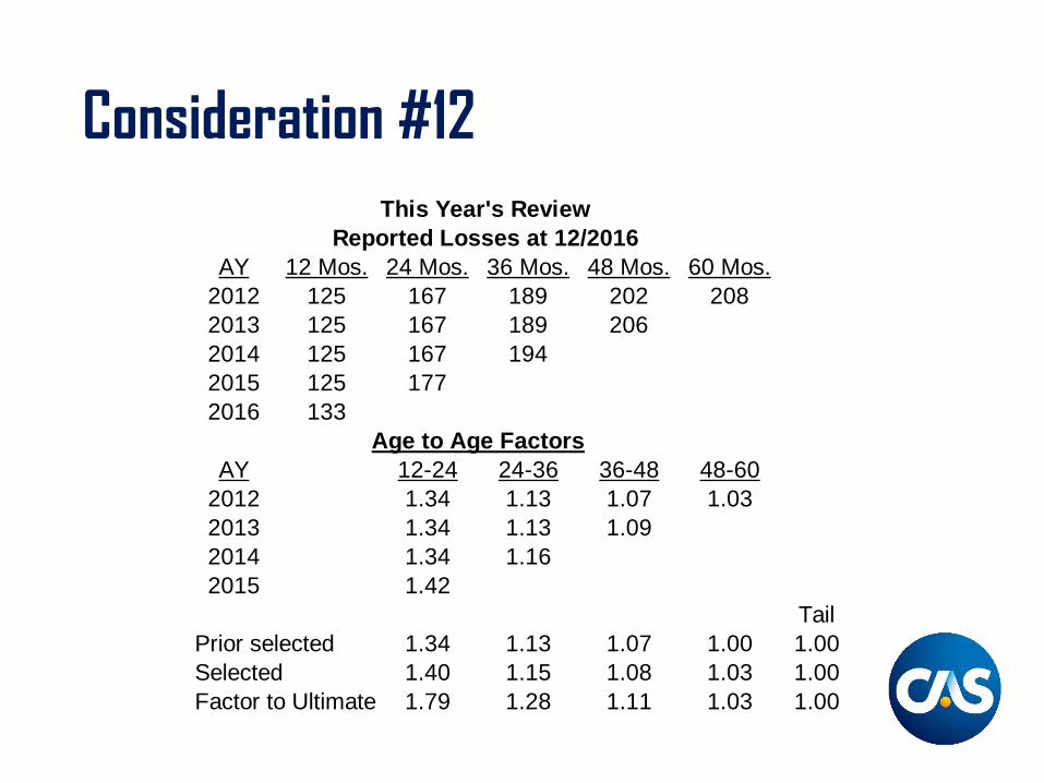
Consideration #12
Reported Losses at 12/2016AY 12 Mos. 24 Mos. 36 Mos. 48 Mos. 60 Mos.
2012 125 167 189 202 2082013 125 167 189 2062014 125 167 1942015 125 1772016 133
Age to Age FactorsAY 12-24 24-36 36-48 48-60
2012 1.34 1.13 1.07 1.032013 1.34 1.13 1.092014 1.34 1.162015 1.42
TailPrior selected 1.34 1.13 1.07 1.00 1.00Selected 1.40 1.15 1.08 1.03 1.00Factor to Ultimate 1.79 1.28 1.11 1.03 1.00
This Year's Review
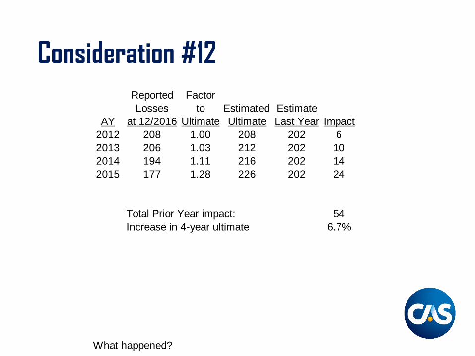
Consideration #12Reported FactorLosses to Estimated Estimate
AY at 12/2016 Ultimate Ultimate Last Year Impact2012 208 1.00 208 202 62013 206 1.03 212 202 102014 194 1.11 216 202 142015 177 1.28 226 202 24
Total Prior Year impact: 54Increase in 4-year ultimate 6.7%
What happened?
Consideration #12
• Did the actuary miss the boat last year? • Did the actuary overreact this year?• What if factors (development assumptions)
remained unchanged?
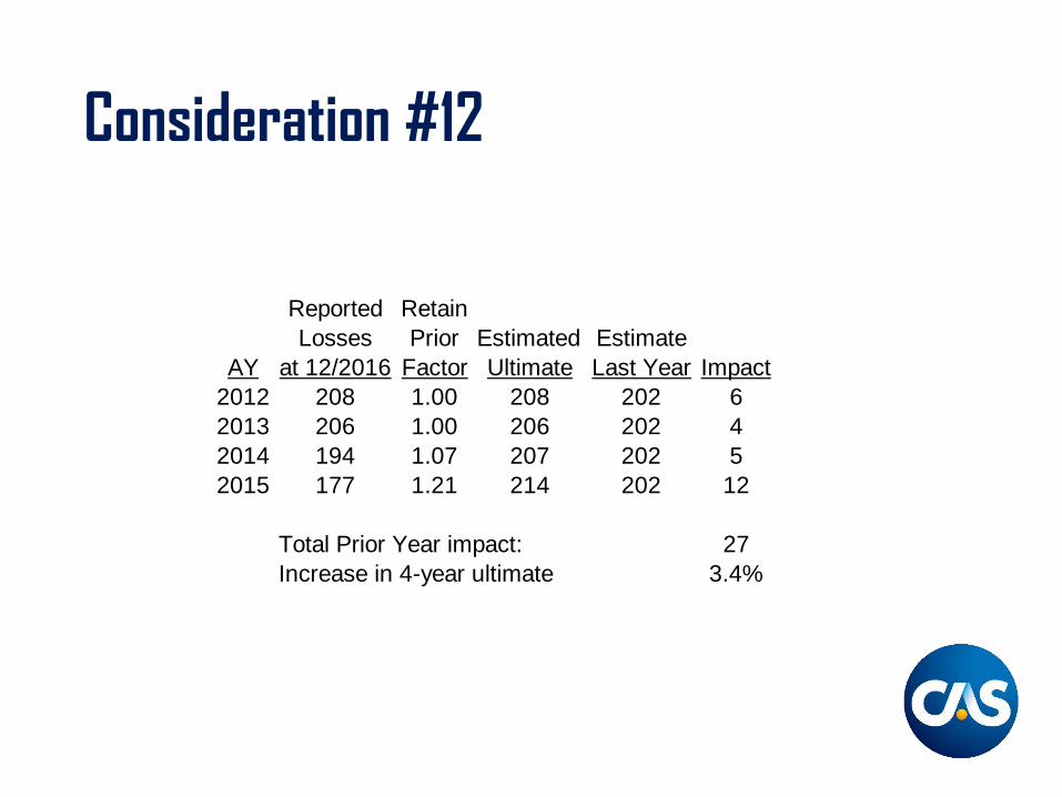
Consideration #12
Reported RetainLosses Prior Estimated Estimate
AY at 12/2016 Factor Ultimate Last Year Impact2012 208 1.00 208 202 62013 206 1.00 206 202 42014 194 1.07 207 202 52015 177 1.21 214 202 12
Total Prior Year impact: 27Increase in 4-year ultimate 3.4%
Consideration #12
• Part of the impact is due to actual losses emerging different from what was expected.
• Should development assumptions change?– If so, that accounts for the remaining impact.
Conclusions
It is seldom sufficient to simply manipulate the numbers. The actuary must actively seek a thorough understanding of...
• ...the loss and claims process• ...the business and the exposures involved
– underwriting– pricing– reinsurance
• …techniques and models to deal with the available data
Conclusions
If professional colleagues are to rely on actuarial advice, they will expect meaningful interpretation of the indications, and the risks and uncertainties in changing estimates.

Investigating and Detecting Change
The Ideal Situation
Loss reserve data should contain a long, stable history of homogeneous claim experience, where no significant operations changes
materially affect either the mix of business or the handling of claims, and there should be a
sufficient number of claims to produce credible loss patterns.

The Reality
• Virtually all elements of “The Ideal” are periodically violated:
1. The Mix Changes2. Claim Handling Changes3. Case Reserves are Strengthened/Weakened4. Other Factors
– Changes in Deductibles, Limits, SIRs– Changes in Reinsurance– Tort Reform, other law changes– New Sources of Loss– Changes in the Economy
We Will Discuss
• The potential impact of mix changes
• Changes in claim closing patterns
• Changes in case reserve adequacy
• What Else?
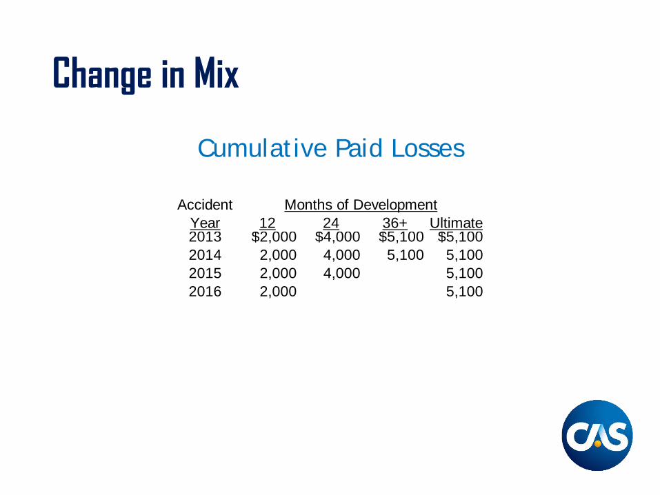
Change in Mix
Cumulative Paid Losses
Accident Months of DevelopmentYear 12 24 36+ Ultimate2013 $2,000 $4,000 $5,100 $5,1002014 2,000 4,000 5,100 5,1002015 2,000 4,000 5,1002016 2,000 5,100
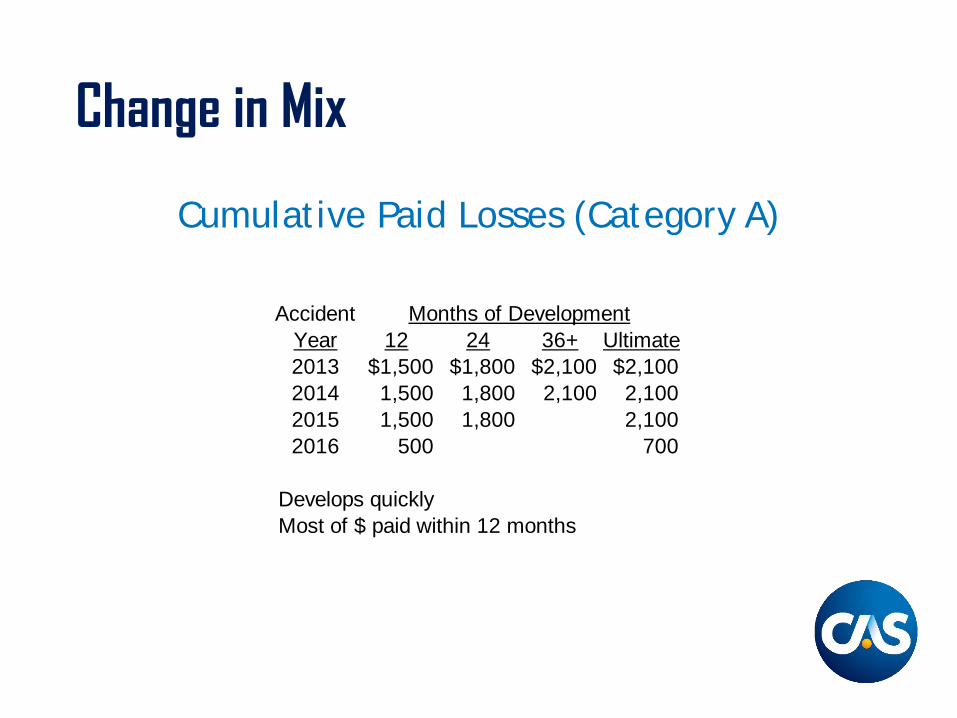
Change in Mix
Cumulative Paid Losses (Category A)
Accident Months of DevelopmentYear 12 24 36+ Ultimate2013 $1,500 $1,800 $2,100 $2,1002014 1,500 1,800 2,100 2,1002015 1,500 1,800 2,1002016 500 700
Develops quicklyMost of $ paid within 12 months
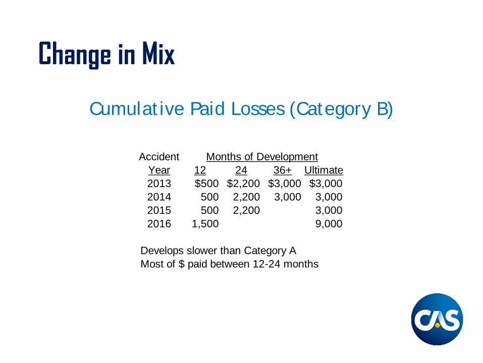
Change in Mix
Cumulative Paid Losses (Category B)
Accident Months of DevelopmentYear 12 24 36+ Ultimate2013 $500 $2,200 $3,000 $3,0002014 500 2,200 3,000 3,0002015 500 2,200 3,0002016 1,500 9,000
Develops slower than Category AMost of $ paid between 12-24 months
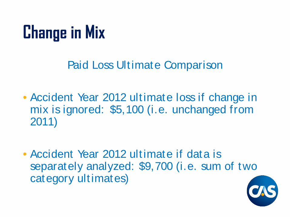
Change in Mix
Paid Loss Ultimate Comparison
• Accident Year 2012 ultimate loss if change in mix is ignored: $5,100 (i.e. unchanged from 2011)
• Accident Year 2012 ultimate if data is separately analyzed: $9,700 (i.e. sum of two category ultimates)
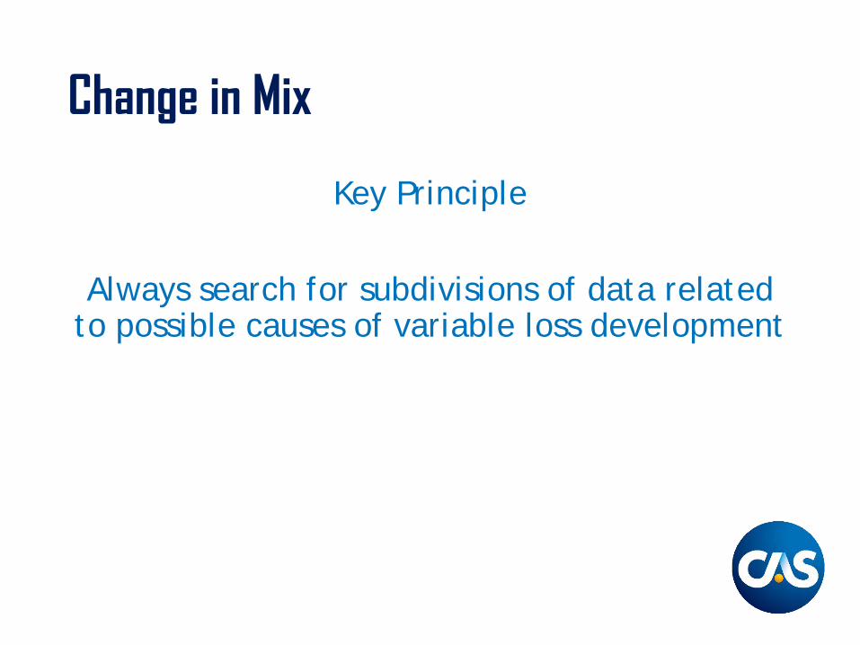
Change in Mix
Key Principle
Always search for subdivisions of data related to possible causes of variable loss development
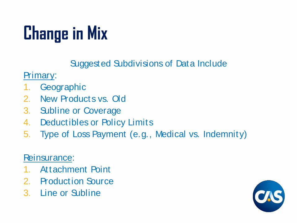
Change in MixSuggested Subdivisions of Data Include
Primary:1. Geographic2. New Products vs. Old3. Subline or Coverage4. Deductibles or Policy Limits5. Type of Loss Payment (e.g., Medical vs. Indemnity)
Reinsurance:1. Attachment Point2. Production Source3. Line or Subline

Change in MixWhat Should be Done if Mix Change Includes New Business
for Which You Have Insufficient Data?Seek Alternative Sources of DataPerhaps general liability book formerly was comprised solely of “OL&T” exposures, but in recent years began adding “M&C” risks. Possible Solution: Relate ISO development patterns for M&C to OL&T and modify development factors for your analysis.Discuss Potential Impacts with Claims, Underwriting, Other Actuaries
– Length of Tail– Frequency– Severity– Loss Ratios
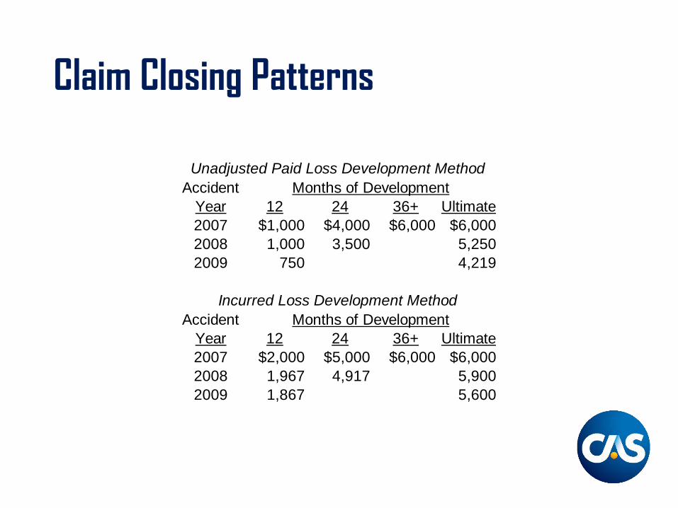
Claim Closing Patterns
Unadjusted Paid Loss Development MethodAccident Months of Development
Year 12 24 36+ Ultimate2007 $1,000 $4,000 $6,000 $6,0002008 1,000 3,500 5,2502009 750 4,219
Incurred Loss Development MethodAccident Months of Development
Year 12 24 36+ Ultimate2007 $2,000 $5,000 $6,000 $6,0002008 1,967 4,917 5,9002009 1,867 5,600
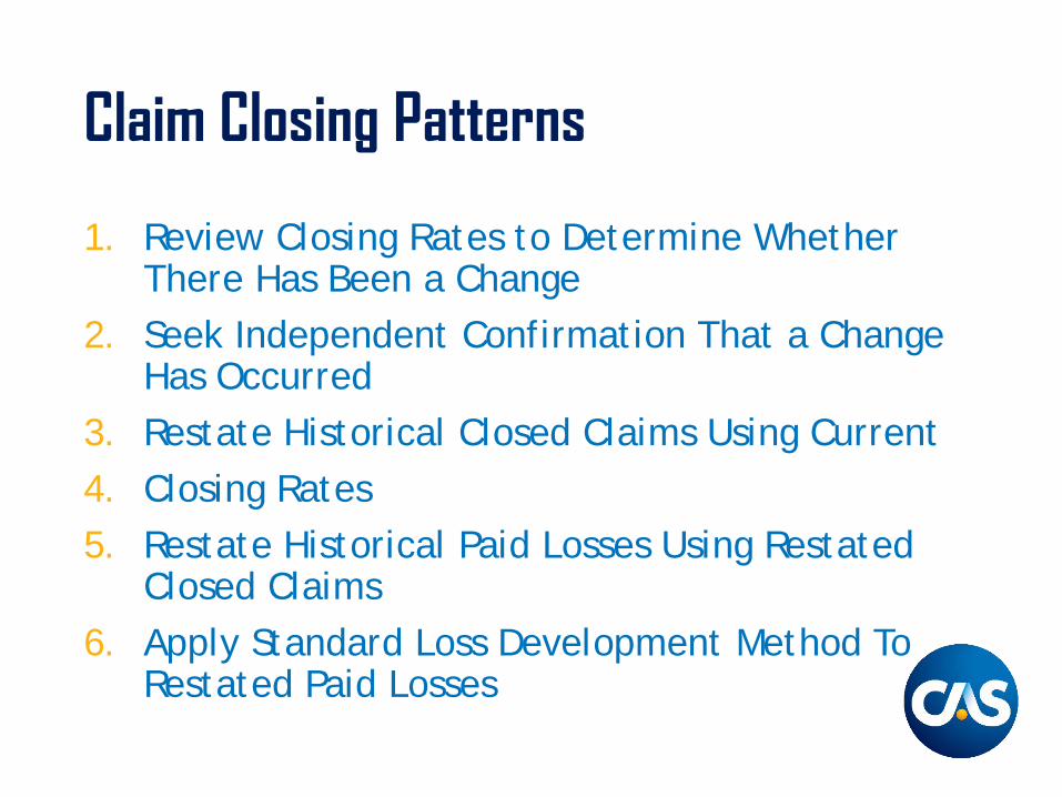
Claim Closing Patterns
1. Review Closing Rates to Determine Whether There Has Been a Change
2. Seek Independent Confirmation That a Change Has Occurred
3. Restate Historical Closed Claims Using Current4. Closing Rates5. Restate Historical Paid Losses Using Restated
Closed Claims6. Apply Standard Loss Development Method To
Restated Paid Losses
Claim Closing Patterns
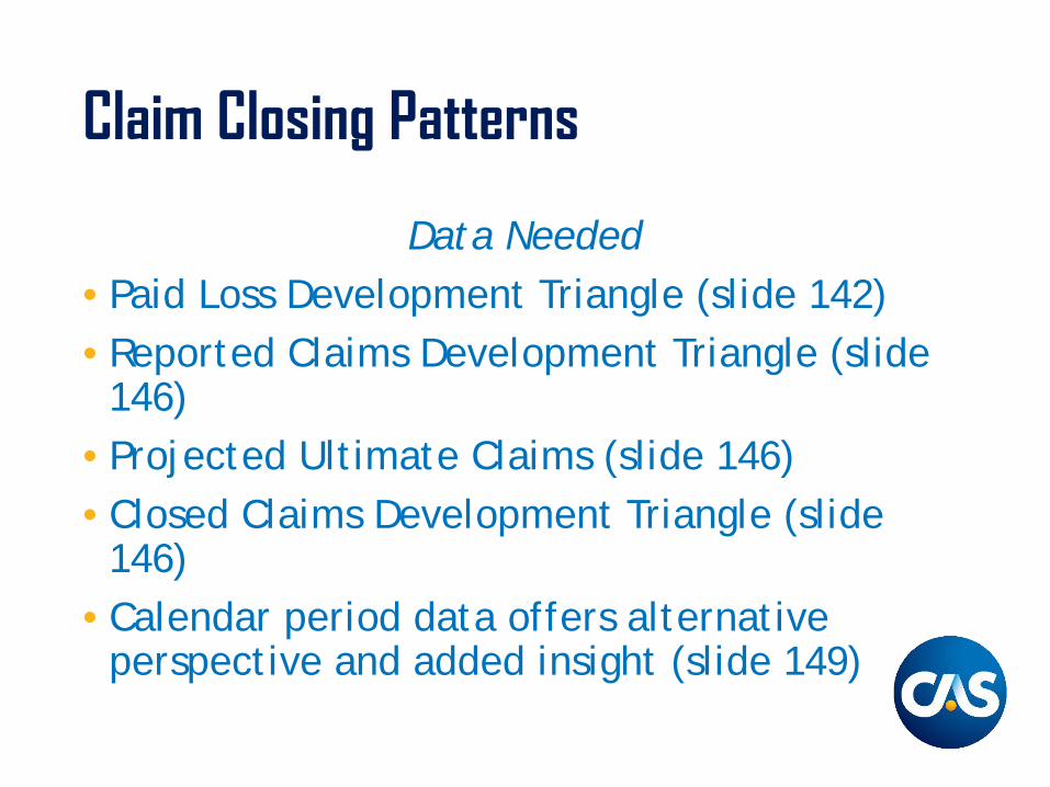
Data Needed• Paid Loss Development Triangle (slide 142)• Reported Claims Development Triangle (slide
146)• Projected Ultimate Claims (slide 146)• Closed Claims Development Triangle (slide
146)• Calendar period data offers alternative
perspective and added insight (slide 149)
Claim Closing Patterns
Step 1: Review Closing Rates to Determine Whether There Has Been a Change
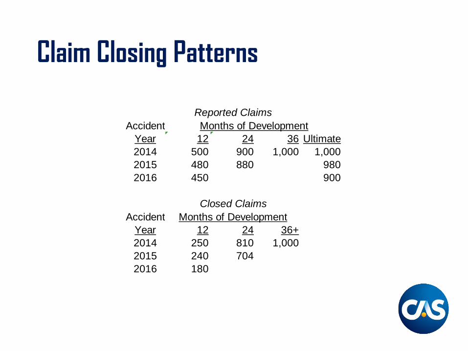
Claim Closing Patterns
Reported ClaimsAccident Months of Development
Year 12 24 36 Ultimate2014 500 900 1,000 1,0002015 480 880 9802016 450 900
Closed ClaimsAccident Months of Development
Year 12 24 36+2014 250 810 1,0002015 240 7042016 180

Claim Closing Patterns
Closed / ReportedAccident Months of Development
Year 12 24 362014 50.0% 90.0% 100.0%2015 50.0% 80.0%2016 40.0%
Closed / UltimateAccident Months of Development
Year 12 24 362014 25.0% 81.0% 100.0%2015 24.5% 71.8%2016 20.0%
Claim Closing Patterns
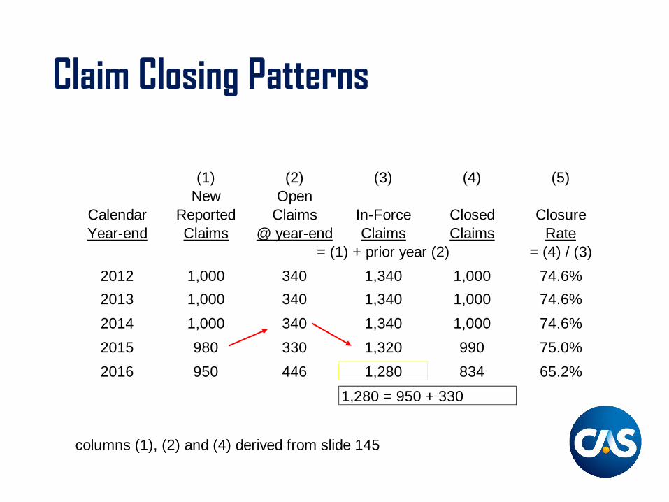
Calendar period data from the Claim Department may also offer a useful tool for monitoring change.
• New Reported Claims• Open Claims• Closed Claims
Claim Closing Patterns
(1) (2) (3) (4) (5)New Open
Calendar Reported Claims In-Force Closed ClosureYear-end Claims @ year-end Claims Claims Rate
= (1) + prior year (2) = (4) / (3)2012 1,000 340 1,340 1,000 74.6%2013 1,000 340 1,340 1,000 74.6%2014 1,000 340 1,340 1,000 74.6%2015 980 330 1,320 990 75.0%2016 950 446 1,280 834 65.2%
1,280 = 950 + 330
columns (1), (2) and (4) derived from slide 145
Claim Closing Patterns
Note that the slowdown in claims closing produces LOWER estimated reserves with the paid development method (will you look a gift horse in the mouth?)
Applies to incurred losses as well
Claim Closing Patterns
Step 2: Seek Independent Confirmation that a Change Has Occurred
Ask the Claims Department About Changes in:– Opening and Closing Practices– The Claims Handling Environment– Levels of Staffing, Reorganizations– Definition of a Claim (e.g., Multiple Claimants)
Claim Closing Patterns
Step 3: Restate Historical Closed Claims Using Current Closing Rates
Claim Closing Patterns
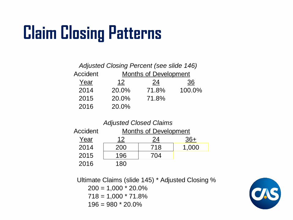
Adjusted Closing Percent (see slide 146)Accident Months of Development
Year 12 24 362014 20.0% 71.8% 100.0%2015 20.0% 71.8%2016 20.0%
Adjusted Closed ClaimsAccident Months of Development
Year 12 24 36+2014 200 718 1,0002015 196 7042016 180
Ultimate Claims (slide 145) * Adjusted Closing % 200 = 1,000 * 20.0% 718 = 1,000 * 71.8% 196 = 980 * 20.0%
Claim Closing Patterns
Step 4: Restate Historical Paid Losses Using Restated Closed Claim
Claim Closing Patterns
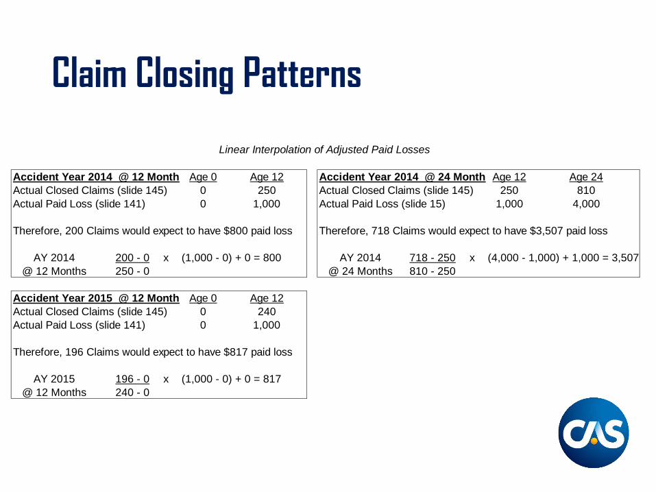
Linear Interpolation of Adjusted Paid Losses
Accident Year 2014 @ 12 Months Age 0 Age 12 Accident Year 2014 @ 24 MonthsAge 12 Age 24Actual Closed Claims (slide 145) 0 250 Actual Closed Claims (slide 145) 250 810Actual Paid Loss (slide 141) 0 1,000 Actual Paid Loss (slide 15) 1,000 4,000
Therefore, 200 Claims would expect to have $800 paid loss Therefore, 718 Claims would expect to have $3,507 paid loss
AY 2014 200 - 0 x (1,000 - 0) + 0 = 800 AY 2014 718 - 250 x (4,000 - 1,000) + 1,000 = 3,507@ 12 Months 250 - 0 @ 24 Months 810 - 250
Accident Year 2015 @ 12 Months Age 0 Age 12Actual Closed Claims (slide 145) 0 240Actual Paid Loss (slide 141) 0 1,000
Therefore, 196 Claims would expect to have $817 paid loss
AY 2015 196 - 0 x (1,000 - 0) + 0 = 817@ 12 Months 240 - 0
Claim Closing Patterns
Step 5: Apply Standard Loss Development Method to Restated Paid Losses
Claim Closing Patterns
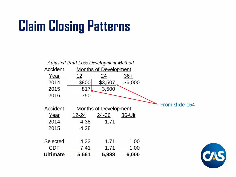
From slide 154
Adjusted Paid Loss Development MethodAccident Months of Development
Year 12 24 36+2014 $800 $3,507 $6,0002015 817 3,5002016 750
Accident Months of DevelopmentYear 12-24 24-36 36-Ult2014 4.38 1.712015 4.28
Selected 4.33 1.71 1.00CDF 7.41 1.71 1.00
Ultimate 5,561 5,988 6,000
Claim Closing Patterns
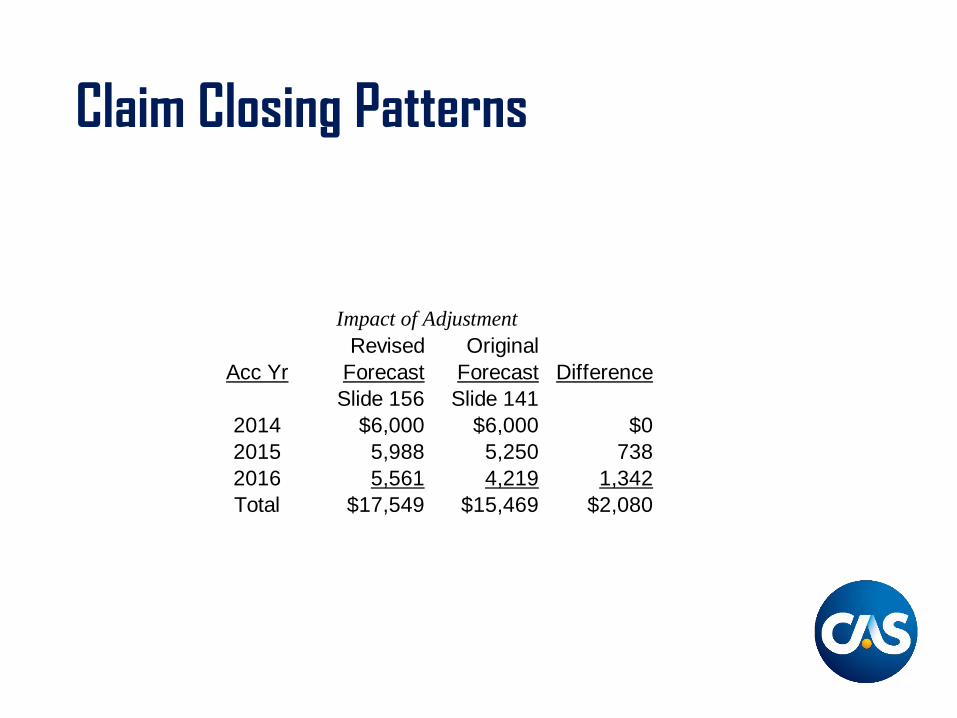
Impact of AdjustmentRevised Original
Acc Yr Forecast Forecast DifferenceSlide 156 Slide 141
2014 $6,000 $6,000 $02015 5,988 5,250 7382016 5,561 4,219 1,342Total $17,549 $15,469 $2,080
Case Reserve Adequacy
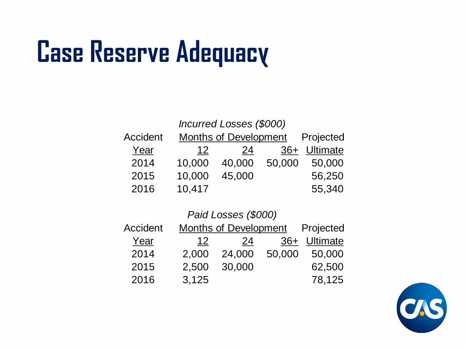
Incurred Losses ($000)Accident Months of Development Projected
Year 12 24 36+ Ultimate2014 10,000 40,000 50,000 50,0002015 10,000 45,000 56,2502016 10,417 55,340
Paid Losses ($000)Accident Months of Development Projected
Year 12 24 36+ Ultimate2014 2,000 24,000 50,000 50,0002015 2,500 30,000 62,5002016 3,125 78,125
Case Reserve Adequacy
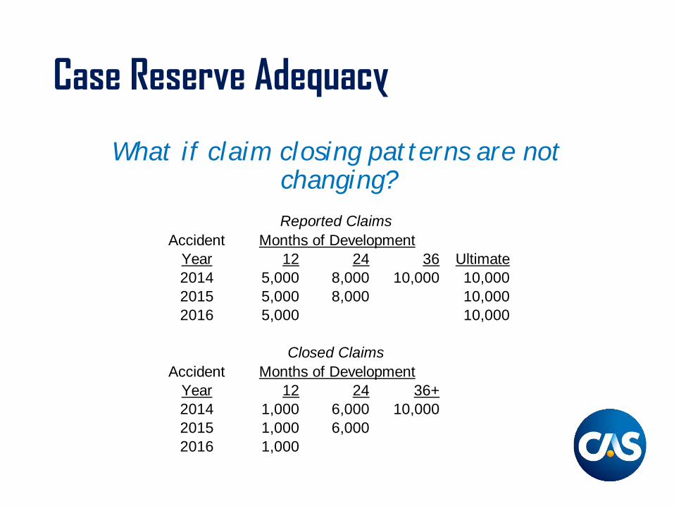
What if claim closing patterns are not changing?Reported Claims
Accident Months of Development Year 12 24 36 Ultimate2014 5,000 8,000 10,000 10,0002015 5,000 8,000 10,0002016 5,000 10,000
Closed ClaimsAccident Months of Development
Year 12 24 36+2014 1,000 6,000 10,0002015 1,000 6,0002016 1,000
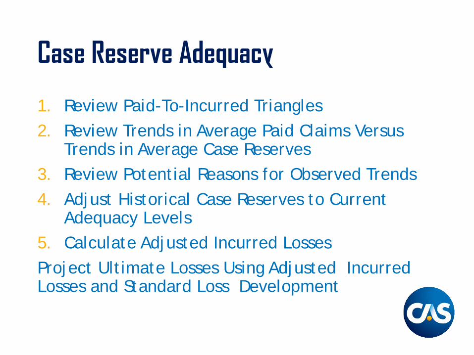
Case Reserve Adequacy
1. Review Paid-To-Incurred Triangles2. Review Trends in Average Paid Claims Versus
Trends in Average Case Reserves3. Review Potential Reasons for Observed Trends4. Adjust Historical Case Reserves to Current
Adequacy Levels5. Calculate Adjusted Incurred LossesProject Ultimate Losses Using Adjusted Incurred Losses and Standard Loss Development
Case Reserve Adequacy
Step 1: Review Paid - To - Incurred Triangles
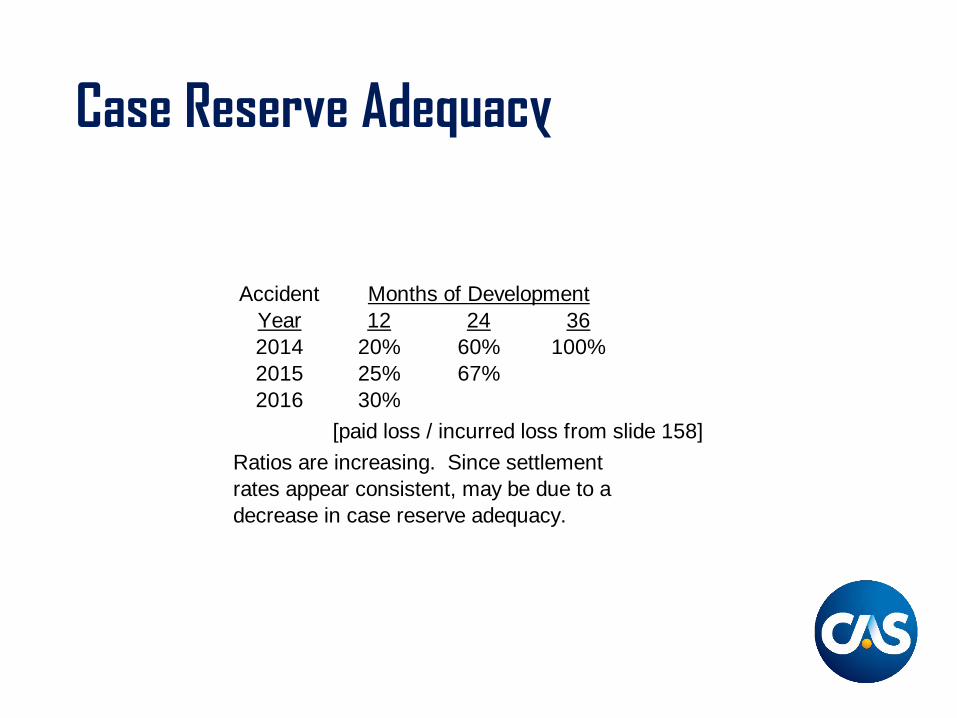
Case Reserve Adequacy
Accident Months of DevelopmentYear 12 24 362014 20% 60% 100%2015 25% 67%2016 30%
[paid loss / incurred loss from slide 158]Ratios are increasing. Since settlementrates appear consistent, may be due to adecrease in case reserve adequacy.
Case Reserve Adequacy
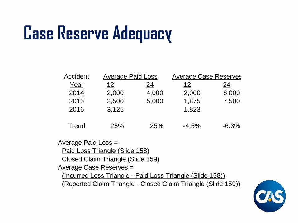
Step 2: Review Trends in Average Paid Claims Versus Trends in Average Case Reserves
Case Reserve Adequacy
Accident Average Paid Loss Average Case ReservesYear 12 24 12 242014 2,000 4,000 2,000 8,0002015 2,500 5,000 1,875 7,5002016 3,125 1,823
Trend 25% 25% -4.5% -6.3%
Average Paid Loss =Paid Loss Triangle (Slide 158)Closed Claim Triangle (Slide 159)
Average Case Reserves =(Incurred Loss Triangle - Paid Loss Triangle (Slide 158))(Reported Claim Triangle - Closed Claim Triangle (Slide 159))
Case Reserve Adequacy
Step 3: Review Potential Reasons for Observed Trends
• Is the book shifting to a lower severity mix?• Have policy limits and/or reinsurance retentions
kept pace with claims inflation?• Has anything material changed in the handling of
claims?• Turnover in claim department staff• Changes in philosophy• If you conclude there has been case reserve
weakening (or strengthening), adjust the data.Here’s one approach.
Case Reserve Adequacy
Step 4: Adjust Historical Case Reserves to Current Adequacy Levels

Case Reserve Adequacy
• Assumption:– 25% is the Actual Rate of Claim Inflation (slide
164)
1,458 = 1,823 / 1.25
Accident Adjusted Average Case ReservesYear 12 24 362014 1,167 6,000 02015 1,458 7,5002016 1,823
1,167 = 1,823 / (1.252)6,000 = 7,500 / 1.25
Case Reserve Adequacy
Step 5: Calculate Adjusted Incurred Losses
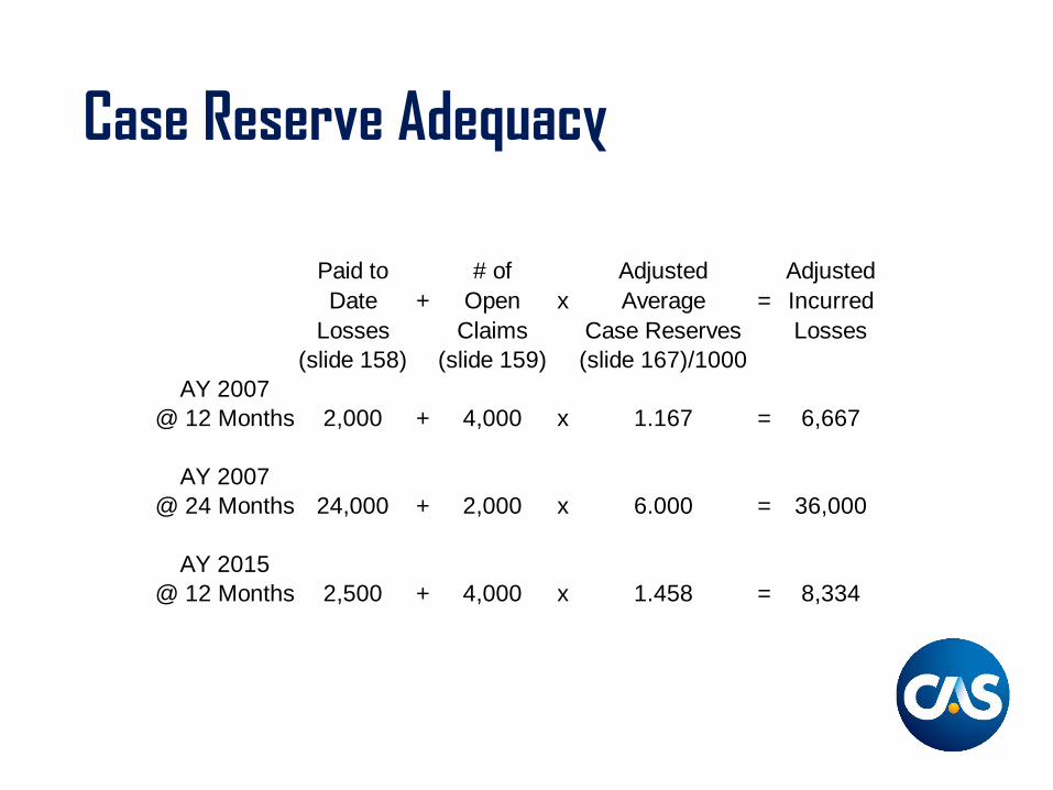
Case Reserve Adequacy
Paid to # of Adjusted AdjustedDate + Open x Average = Incurred
Losses Claims Case Reserves Losses(slide 158) (slide 159) (slide 167)/1000
AY 2007@ 12 Months 2,000 + 4,000 x 1.167 = 6,667
AY 2007@ 24 Months 24,000 + 2,000 x 6.000 = 36,000
AY 2015@ 12 Months 2,500 + 4,000 x 1.458 = 8,334
Case Reserve Adequacy
Step 6: Project Ultimate Losses Using Adjusted Incurred Losses and Standard Loss Development
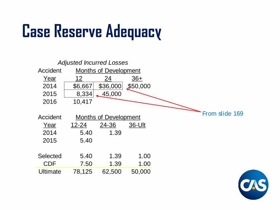
Case Reserve Adequacy
From slide 169
Adjusted Incurred LossesAccident Months of Development
Year 12 24 36+2014 $6,667 $36,000 $50,0002015 8,334 45,0002016 10,417
Accident Months of DevelopmentYear 12-24 24-36 36-Ult2014 5.40 1.392015 5.40
Selected 5.40 1.39 1.00CDF 7.50 1.39 1.00
Ultimate 78,125 62,500 50,000
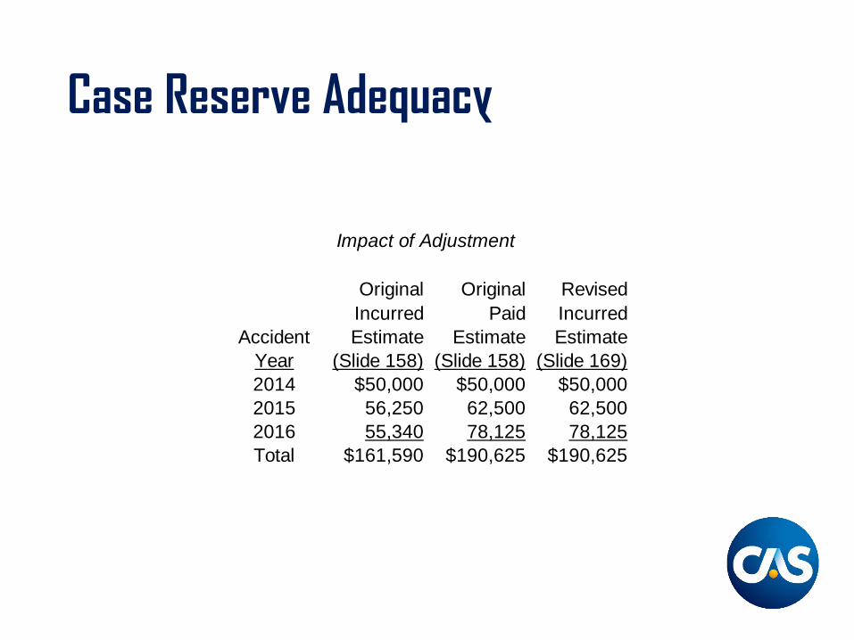
Case Reserve Adequacy
Impact of Adjustment
Original Original RevisedIncurred Paid Incurred
Accident Estimate Estimate EstimateYear (Slide 158) (Slide 158) (Slide 169)2014 $50,000 $50,000 $50,0002015 56,250 62,500 62,5002016 55,340 78,125 78,125Total $161,590 $190,625 $190,625
What Else?
• Deductibles/Limits/SIRs change• Reinsurance Arrangements Change• Tort Reform• New Sources of Loss• Changes in the Economy
Deductibles/Limits/SIRs change
• Deductibles may change the number of claims• May change loss $ as well• Need to review profile of deductibles and
limits – inherent assumption is no change• Treat like change in mix
Reinsurance Arrangements Change
• Effect on total net liability• Might also affect claims handling• e.g., if retention is limited to $100,000 by
reinsurance, is there an incentive to settle a• $500,000 case more quickly than if you were
on the hook for the whole thing?
Tort Reform
• Change in benefits which would affect severity and payout (e.g. cost containment)
• Change in statute of limitations (frequency change, less “tail” development)
• New patterns – e.g., ability to do lump-sum settlements of permanent workers’ comp claims

New Sources of Loss
• Mold• Terrorism• Asbestos – just keeps on running• Stacking of auto limits
Summary
Assumption of long, stable history is often violated.
• The mix of business can change
• Claim closing patterns can change
• Case reserve adequacy can change
• Other factors can change as well