basic plasma physics - descanso

37

Chapter 3

Basic Plasma Physics

3.1 Introduction

Electric propulsion achieves high specific impulse by the acceleration of

charged particles to high velocity. The charged particles are produced by

ionization of a propellant gas, which creates both ions and electrons and forms

what is called a plasma. Plasma is then a collection of the various charged

particles that are free to move in response to fields they generate or fields that

are applied to the collection and, on the average, is almost electrically neutral.

This means that the ion and electron densities are nearly equal, ni ne , a

condition commonly termed “quasi-neutrality.” This condition exists

throughout the volume of the ionized gas except close to the boundaries, and

the assumption of quasi-neutrality is valid whenever the spatial scale length of

the plasma is much larger than the characteristic length over which charges or

boundaries are electrostatically shielded, called the Debye length. The ions and

electrons have distributions in energy usually characterized by a temperature Ti

for ions and Te for electrons, which are not necessarily or usually the same. In

addition, different ion and electron species can exist in the plasma with

different temperatures or different distributions in energy.

Plasmas in electric propulsion devices, even in individual parts of a thruster,

can span orders of magnitude in plasma density, temperature, and ionization

fraction. Therefore, models used to describe the plasma behavior and

characteristics in the thrusters must be formed with assumptions that are valid

in the regime being studied. Many of the plasma conditions and responses in

thrusters can be modeled by fluid equations, and kinetic effects are only

important in specific instances.

There are several textbooks that provide very comprehensive introductions to

plasma physics [1–3] and the generation of ion beams [4]. This chapter is

38 Chapter 3

intended to provide the basic plasma physics necessary to understand the

operation of ion and Hall thrusters. The units used throughout the book are

based on the International System (SI). However, by convention we will

occasionally revert to other metric units (such as A/cm2, mg/s, etc.) commonly

used in the literature describing these devices.

3.2 Maxwell’s Equations

The electric and magnetic fields that exist in electric propulsion plasmas obey

Maxwell’s equations formulated in a vacuum that contains charges and

currents. Maxwell’s equations for these conditions are

E =o

(3.2-1)

E =Bt

(3.2-2)

B = 0 (3.2-3)

B = μo J + oEt

, (3.2-4)

where is the charge density in the plasma, J is the current density in the

plasma, and o and μo are the permittivity and permeability of free space,

respectively. Note that and J comprise all the charges and currents for all the

particle species that are present in the plasma, including multiply charged ions.

The charge density is then

= qsns = e Zni ne( )s

, (3.2-5)

where qs is the charge state of species s, Z is the charge state, ni is the ion

number density, and ne is the electron number density. Likewise, the current

density is

J = qsnsvs = e Znivi neve( )s

, (3.2-6)

where vs is the velocity of the charge species, vi is the ion velocity, and ve is

the electron velocity. For static magnetic fields B t = 0( ) , the electric field

can be expressed as the gradient of the electric potential,

Basic Plasma Physics 39

E = , (3.2-7)

where the negative sign comes from the convention that the electric field

always points in the direction of ion motion.

3.3 Single Particle Motions

The equation of motion for a charged particle with a velocity v in a magnetic

field B is given by the Lorentz force equation:

F = mdvdt

= q E + v B( ) . (3.3-1)

Particle motion in a magnetic field in the ˆ z direction for the case of negligible

electric field is found by evaluating Eq. (3.3-1):

mvx

t= qBvy

mvy

t= –qBvx

mvz

t= 0.

(3.3-2)

Taking the time derivative of Eq. (3.3-2) and solving for the velocity in each

direction gives

2vx

t2=

qB

m

vy

t=

qB

m

2

vx

2vy

t2=

qB

m

vx

t=

qB

m

2

vy .

(3.3-3)

These equations describe a simple harmonic oscillator at the cyclotron

frequency:

c =q B

m. (3.3-4)

For electrons, this is called the electron cyclotron frequency.

The size of the particle orbit for finite particle energies can be found from the

solution to the particle motion equations in the axial magnetic field. In this

case, the solution to Eq. (3.3-3) is

40 Chapter 3

vx,y = v ei ct . (3.3-5)

The equation of motion in the y-direction in Eq. (3.3-2) can be rewritten as

vy =m

qB

vx

t=

1

c

vx

t. (3.3-6)

Utilizing Eq. (3.3-5), Eq. (3.3-6) becomes

vy =1

c

vx

t= iv ei ct =

y

t. (3.3-7)

Integrating this equation gives

y yo =v

cei ct . (3.3-8)

Taking the real part of Eq. (3.3-8) gives

y yo =v

ccos ct = rL cos ct , (3.3-9)

where rL = v / c is defined as the Larmor radius. A similar analysis of the

displacement in the x direction gives the same Larmor radius 90 degrees out of

phase with the y -direction displacement, which then with Eq. (3.3-9) describes

the particle motion as a circular orbit around the field line at xo and yo with a

radius given by rL .

The Larmor radius arises from very simple physics. Consider a charged particle

of mass, m, in a uniform magnetic field with a velocity in one direction, as

illustrated in Fig. 3-1. The charge will feel a Lorentz force

F = qv B . (3.3-10)

Since the charged particle will move under this force in circular orbits in the

v B direction, it feels a corresponding centripetal force such that


��

�

�

�

Fig. 3-1. Positively charged particle

moving in a uniform vertical magnetic field.

Fc = qv B =mv2

r, (3.3-11)

where r is the radius of the cycloidal motion

in the magnetic field. Solving for the radius

of the circle gives

r = rL =mv

qB, (3.3-12)

which is the Larmor radius.

The Larmor radius can be written in a form

simple to remember:

rL =v

c=

1

B

2mV

e, (3.3-13)

using 1 2mv2= eV for the singly charged particle energy in the direction

perpendicular to the magnetic field. The direction of particle gyration is always

such that the induced magnetic field is opposite in direction to the applied field,

which tends to reduce the applied field, an effect called diamagnetism. Any

particle motion along the magnetic field is not affected by the field, but causes

the particle motion to form a helix along the magnetic field direction with a

radius given by the Larmor radius and a pitch given by the ratio of the

perpendicular to parallel velocities.

Next consider the situation in Fig. 3-1, but with the addition of a finite electric

field perpendicular to B. In this case, E is in some direction in the plane of the

page. The equation of motion for the charged particle is given by Eq. (3.3-1).

Considering the drift to be steady-state, the time derivative is equal to zero, and

Eq. (3.3-1) becomes

E = v B . (3.3-14)

Taking the cross product of both sides with B gives

E B = v B( ) B = vB2 B B v( ) . (3.3-15)

The dot product is in the direction perpendicular to B, so the last term in

Eq. (3.3-15) is equal to zero. Solving for the transverse velocity of the particle

gives

42 Chapter 3

v =E B

B2vE , (3.3-16)

which is the “E cross B” drift velocity. In this case, the drift is in the direction

perpendicular to both E and B, and arises from the cycloidal electron motion in

the magnetic field being accelerated in the direction of –E and decelerated in

the direction of E. This elongates the orbit on one-half cycle and shrinks the

orbit on the opposite half cycle, which causes the net motion of the particle in

the E B direction. The units of the E B velocity are

vE =E [V/ m]

B [tesla] (m/ s) . (3.3-17)

Finally, consider the situation of a particle gyrating in a magnetic field that is

changing in magnitude along the magnetic field direction ˆ z . This is commonly

found in electric propulsion thrusters relatively close to permanent magnets or

electromagnetic poles-pieces that produce fields used to confine the electrons.

Since the divergence of B is zero, Eq. (3.2-3), the magnetic field in cylindrical

coordinates is described by

1

r rrBr( ) +

Bz

z= 0 . (3.3-18)

Assuming that the axial component of the field does not vary significantly with

r and integrating yields the radial component of the magnetic field with respect

to r,

Brr

2

Bz

z. (3.3-19)

The Lorentz force on a charged particle has a component along ˆ z given by

Fz qv Br , (3.3-20)

where the azimuthal particle velocity averaged over a Larmor-radius ( r = rL )

gyration is v = v . The average force on the particle is then

F z1

2

mv2

B

Bz

z. (3.3-21)

The magnetic moment of the gyrating particle is defined as


μ =1

2

mv2

B. (3.3-22)

As the particle moves along the magnetic field lines into a stronger magnitude

field, the parallel energy of the particle is converted into rotational energy and

its Larmor radius increases. However, its magnetic moment remains invariant

because the magnetic field does no work and the total kinetic energy of the

particle is conserved. For a sufficiently large increase in the field, a situation

can arise where the parallel velocity of the particle goes to zero and the Lorentz

force reflects the particle from a “magnetic mirror.” By conservation of energy,

particles will be reflected from the magnetic mirror if their parallel velocity is

less than

v|| < v Rm 1 , (3.3-23)

where v|| is the parallel velocity and Rm is the mirror ratio given by

Bmax / Bmin . This effect is used to provide confinement of energetic electrons

in ion-thruster discharge chambers.

There are a number of other particle drifts and motions possible that depend on

gradients in the magnetic and electric fields, and also on time-dependent or

oscillating electric or magnetic fields. These are described in detail in plasma

physics texts such as Chen [1], and while they certainly might occur in the

electric propulsion devices considered here, they are typically not of critical

importance to the thruster performance or behavior.

3.4 Particle Energies and Velocities

In ion and Hall thrusters, the charge particles may undergo a large number of

collisions with each other, and in some cases with the other species (ions,

electrons, and/or neutrals) in the plasma. It is therefore impractical to analyze

the motion of each particle to obtain a macroscopic picture of the plasma

processes that is useful to for assessing the performance and life of these

devices. Fortunately, in most cases it is not necessary to track individual

particles to understand the plasma dynamics. The effect of collisions is to

develop a distribution of the velocities for each species. On the average, and in

the absence of other forces, each particle will then move with a speed that is

solely a function of the macroscopic temperature and mass of that species. The

charged particles in the thruster, therefore, can usually be described by different

velocity distribution functions, and the random motions can be calculated by

taking the moments of those distributions.

44 Chapter 3

Most of the charged particles in electric thrusters have a Maxwellian velocity

distribution, which is the most probable distribution of velocities for a group of

particles in thermal equilibrium. In one dimension, the Maxwellian velocity

distribution function is

f (v) =m

2 kT

1/2

expmv2

2kT, (3.4-1)

where m is the mass of the particle, k is Boltzmann’s constant, and the width of

the distribution is characterized by the temperature T. The average kinetic

energy of a particle in the Maxwellian distribution in one dimension is

Eave =

12

mv2 f (v) dv–

f (v) dv–

. (3.4-2)

By inserting in Eq. (3.4-1) and integrating by parts, the average energy per

particle in each dimension is

Eave =1

2kT . (3.4-3)

If the distribution function is generalized into three dimensions, Eq. (3.2-8)

becomes

f (u,v,w) =m

2 kT

3/2

expm

2kTu2+v2+w2( ) , (3.4-4)

where u, v, and w represent the velocity components in the three coordinate

axes. The average energy in three dimensions is found by inserting Eq. (3.4-2)

in Eq. (3.4-4) and performing the triple integration to give

Eave =3

2kT . (3.4-5)

The density of the particles is found from

n = nf (v) dv–

+

= nm

2 kT

3/2

expm u2+v2+w2( )

2kTdudvdw

–

+.

(3.4-6)


The average speed of a particle in the Maxwellian distribution is

v = v0

m

2 kT

3/2

exp –v2

vth2

4 v2dv , (3.4-7)

where v in Eq. (3.4-7) denotes the particle speed and vth is defined as

(2kT / m)1/2 . Integrating Eq. (3.4-7), the average speed per particle is

v =8kT

m

1/2

. (3.4-8)

The flux of particles in one dimension (say in the ˆ z direction) for a Maxwellian

distribution of particle velocities is given by n < vz > . In this case, the average

over the particle velocities is taken in the positive vz direction because the flux

is considered in only one direction. The particle flux (in one direction) is then

z = nvz f (v)d3v , (3.4-9)

which can be evaluated by integrating the velocities in spherical coordinates

with the velocity volume element given by

d 3v = v2dvd = v2dv sin d d , (3.4-10)

where the d represents the element of the solid angle. If the incident velocity

has a cosine distribution ( vz = vcos ), the one-sided flux is

z = n m

2 kT

3/2

d0

2sin d

0

/2 v cos exp –

v2

vth0v2dv , (3.4-11)

which gives

z =1

4nv =

1

4n

8kT

m

1/2

. (3.4-12)

Since the plasma electrons are very mobile and tend to make a large number of

coulomb collisions with each other, they can usually be characterized by a

Maxwellian temperature Te and have average energies and speeds well

described by the equations derived in this section. The random electron flux

inside the plasma is also well described by Eq. (3.4-12) if the electron

46 Chapter 3

temperature and density are known. The electrons tend to be relatively hot

(compared to the ions and atoms) in ion and Hall thrusters because they

typically are injected into the plasma or heated by external mechanisms to

provide sufficient energy to produce ionization. In the presence of electric and

magnetic fields in the plasma and at the boundaries, the electron motion will no

longer be purely random, and the flux described by Eq. (3.4-12) must be

modified as described in the remainder of this chapter.

The ions in thrusters, on the other hand, are usually relatively cold in

temperature (they may have high directed velocities after being accelerated, but

they usually have low random velocities and temperatures). This occurs

because the ions are not well confined in the plasma generators because they

must be extracted to form the thrust beam, and so they leave the plasma after

perhaps only a single pass. The ions are also not heated efficiently by the

various mechanisms used to ionize the gas. Therefore, the plasmas in ion and

Hall thrusters are usually characterized as having cold ions and Maxwellian

electrons with a high electron-to-ion temperature ratio (Te /Ti 10 ). As a

result, the velocity of the ions in the plasma and the fluxes to the boundaries

tend to be determined by the electric fields generated inside the plasma to

conserve charge, and to be different from the expressions derived here for the

electron velocity and fluxes. This effect will be described in more detail in

Section 3.6.

3.5 Plasma as a Fluid

The behavior of most of the plasma effects in ion and Hall thrusters can be

described by simplified models in which the plasma is treated as a fluid of

neutral particles and electrical charges with Maxwellian distribution functions,

and the interactions and motion of only the fluid elements must be considered.

Kinetic effects that consider the actual velocity distribution of each species are

important in some instances, but will not be addressed here.

3.5.1 Momentum Conservation

In constructing a fluid approach to plasmas, there are three dominant forces on

the charged particles in the plasma that transfer momentum that are considered

here. First, charged particles react to electric and magnetic field by means of the

Lorentz force, which was given by Eq. (3.3-1):

FL = mdvdt

= q E + v B( ) . (3.5-1)

Next, there is a pressure gradient force,


Fp = –p

n= –

nkT( )

n, (3.5-2)

where the pressure is given by P = nkT and should be written more rigorously

as a stress tensor since it can, in general, be anisotropic. For plasmas with

temperatures that are generally spatially constant, the force due to the pressure

gradient is usually written simply as

Fp = –kTn

n. (3.5-3)

Finally, collisions transfer momentum between the different charged particles,

and also between the charged particles and the neutral gas. The force due to

collisions is

Fc = –m ab va – vb( )a,b

, (3.5-4)

where vab is the collision frequency between species a and b.

Using these three force terms, the fluid momentum equation for each species is

mndvdt

= mnvt

+ v( )v = qn E+v B( ) – p – mn v – vo( ) , (3.5-5)

where the convective derivative has been written explicitly and the collision

term must be summed over all collisions.

Utilizing conservation of momentum, it is possible to evaluate how the electron

fluid behaves in the plasma. For example, in one dimension and in the absence

of magnetic fields and collisions with other species, the fluid equation of

motion for electrons can be written as

mnevz

t+ v( )vz = qneEz –

p

z, (3.5-6)

where vz is the electron velocity in the z-direction and p represents the electron

pressure term. Neglecting the convective derivative, assuming that the velocity

is spatially uniform, and using Eq. (3.5-3) gives

mvz

t= –eEz –

kTe

ne

ne

z. (3.5-7)

48 Chapter 3

Assuming that the electrons have essentially no inertia (their mass is small and

so they react infinitely fast to changes in potential), the left-hand side of

Eq. (3.5-7) goes to zero, and the net current in the system is also zero.

Considering only electrons at a temperature Te , and using Eq. (3.2-7) for the

electric field, gives

qEz = ez

=kTe

ne

ne

z. (3.5-8)

Integrating this equation and solving for the electron density produces the

Boltzmann relationship for electrons:

ne = ne(0) e e /kTe( ), (3.5-9)

where is the potential relative to the potential at the location of ne(0) .

Equation (3.5-9) is also sometimes known as the barometric law. This

relationship simply states that the electrons will respond to electrostatic fields

(potential changes) by varying their density to preserve the pressure in the

system. This relationship is generally valid for motion along a magnetic field

and tends to hold for motion across magnetic fields if the field is weak and the

electron collisions are frequent.

3.5.2 Particle Conservation

Conservation of particles and/or charges in the plasma is described by the

continuity equation:

n

t+ nv = ns , (3.5-10)

where ns represents the time-dependent source or sink term for the species

being considered. Continuity equations are sometimes called mass-conservation

equations because they account for the sources and sinks of particles into and

out of the plasma.

Utilizing continuity equations coupled with momentum conservation and with

Maxwell’s equations, it is possible to calculate the response rate and wave-like

behavior of plasmas. For example, the rate at which a plasma responds to

changes in potential is related to the plasma frequency of the electrons. Assume

that there is no magnetic field in the plasma or that the electron motion is along

the magnetic field in the z-direction. To simplify this derivation, also assume

that the ions are fixed uniformly in space on the time scales of interest here due

to their large mass, and that there is no thermal motion of the particles (T = 0).


Since the ions are fixed in this case, only the electron equation of motion is of

interest:

mnevz

t+ v( )vz = –eneEz , (3.5-11)

and the electron equation of continuity is

ne

t+ nev( ) = 0 . (3.5-12)

The relationship between the electric field and the charge densities is given by

Eq. (3.2-1), which for singly ionized particles can be written using Eq. (3.2-5)

as

E =o

=e

oni – ne( ) . (3.5-13)

The wave-like behavior of this system is analyzed by linearization using

E = Eo + E1 (3.5-14)

v = vo + v1 (3.5-15)

n = no + n1 , (3.5-16)

where Eo , vo , and no are the equilibrium values of the electric field, electron

velocity, and electron density, and E1 , B1 , and j1 are the perturbed values of

these quantities. Since quasi-neutral plasma has been assumed, Eo = 0 , and the

assumption of a uniform plasma with no temperature means that no = vo = 0 .

Likewise, the time derivatives of these equilibrium quantities are zero.

Linearizing Eq. (3.5-13) gives

E1 = –e

on1 . (3.5-17)

Using Eqs. (3.5-14), (3.5-15), and (3.5-16) in Eq. (3.5-11) results in

dv1

dt= –

e

mE1 z , (3.5-18)

50 Chapter 3

where the linearized convective derivative has been neglected. Linearizing the

continuity Eq. (3.5-12) gives

dn1

dt= –no v1 z , (3.5-19)

where the quadratic terms, such as n1v1 , etc., have been neglected as small. In

the linear regime, the oscillating quantities will behave sinusoidally:

E1 = E1 ei(kz– t ) z (3.5-20)

v1 = v1 ei(kz– t ) z (3.5-21)

n1 = n1 ei(kz– t ) . (3.5-22)

This means that the time derivates in momentum and continuity equations can

be replaced by i t , and the gradient in Eq. (3.5-17) can be replaced by ik in

the ˆ z direction. Combining Eqs. (3.5-17), (3.5-18), and (3.5-19), using the time

and spatial derivatives of the oscillating quantities, and solving for the

frequency of the oscillation gives

p =nee

2

om

1/2

, (3.5-23)

where p is the electron plasma frequency. A useful numerical formula for the

electron plasma frequency is

fp =p

29 ne , (3.5-24)

where the plasma density is in m–3

. This frequency is one of the fundamental

parameters of a plasma, and the inverse of this value is approximately the

minimum time required for the plasma to react to changes in its boundaries or

in the applied potentials. For example, if the plasma density is 1018

m–3

, the

electron plasma frequency is 9 GHz, and the electron plasma will respond to

perturbations in less than a nanosecond.

In a similar manner, if the ion temperature is assumed to be negligible and the

gross response of the plasma is dominated by ion motions, the ion plasma

frequency can be found to be


p =nee

2

oM

1/2

. (3.5-25)

This equation provides the approximate time scale in which ions move in the

plasma. For our previous example for a 1018

m–3

plasma density composed of

xenon ions, the ion plasma frequency is about 18 MHz, and the ions will

respond to first order in a fraction of a microsecond. However, the ions have

inertia and respond at the ion acoustic velocity given by

va = ikTi + kTe

M, (3.5-26)

where i is the ratio of the ion specific heats and is equal to one for isothermal

ions. In the normal case for ion and Hall thrusters, where Te >> Ti , the ion

acoustic velocity is simply

va =kTe

M. (3.5-27)

It should be noted that if finite-temperature electrons and ions had been

included in the derivations above, the electron-plasma and ion-plasma

oscillations would have produced waves that propagate with finite wavelengths

in the plasma. Electron-plasma waves and ion-plasma waves (sometimes called

ion acoustic waves) occur in most electric thruster plasmas with varying

amplitudes and effects on the plasma behavior. The dispersion relationships for

these waves, which describe the relationship between the frequency and the

wavelength of the wave, are derived in detail in plasma textbooks such as Chen

[1] and will not be re-derived here.

3.5.3 Energy Conservation

The general form of the energy equation for charged species “s,” moving with

velocity vs in the presence of species “n” is given by

t

nsmsvs

2

2+

3

2ps + nsms

vs2

2+

5

2ps vs + s

= qsns E +Rs

qsnsvs + Qs s .

(3.5-28)

For simplicity, Eq. (3.5-28) neglects viscous heating of the species. The

divergence terms on the left-hand side represent the total energy flux, which

52 Chapter 3

includes the work done by the pressure, the macroscopic energy flux, and the

transport of heat by conduction s = s Ts . The thermal conductivity of the

species is denoted by s , which is given in SI units [5] by

s = 3.2 e ne2TeV

m, (3.5-29)

where TeV in this equation is in electron volts (eV). The right-hand side of

Eq. (3.5-28) accounts for the work done by other forces as well for the

generation/loss of heat as a result of collisions with other particles. The term

Rs represents the mean change in the momentum of particles “s” as a result of

collisions with all other particles:

Rs Rsnn

= nsms sn vs vn( )n

. (3.5-30)

The heat-exchange terms are Qs , which is the heat generated/lost in the

particles of species “s” as a result of elastic collisions with all other species, and

s , the energy loss by species “s” as a result of inelastic collision processes

such as ionization and excitation.

It is often useful to eliminate the kinetic energy from Eq. (3.5-28) to obtain a

more applicable form of the energy conservation law. The left-hand side of

Eq. (3.5-28) is expanded as

nsmsvsDvs

Dt+

msvs2

2

Dns

Dt+ nsms

vs2

2vs +

3

2

ps

t+

5

2psvs + s

= qsnsE vs + Rs vs + Qs s .

(3.5-31)

The continuity equation for the charged species is in the form

Dns

Dt=

ns

t+ vs ns = ˙ n ns vs . (3.5-32)

Combining these two equations with the momentum equation dotted with vs

gives

nsmsvsDv s

Dt= nsqsvs E vs ps + vs Rs ˙ n msvs

2. (3.5-33)

The energy equation can now be written as


3

2

ps

t+

5

2psvs + s vs ps = Qs s n

msvs2

2. (3.5-34)

The heat-exchange terms for each species Qs consists of “frictional” (denoted

by superscript R) and “thermal” (denoted by superscript T) contributions:

Qs = QsR

+ QsT ,

QsR Rsn vs

n

,

QsT ns

2ms

masn

3

2

kTs

e

kTn

en

.

(3.5-35)

In a partially ionized gas consisting of electrons, singly charged ions, and

neutrals of the same species, the frictional and thermal terms for the electrons

take the form

Qe

R= Rei + Ren( ) ve =

Rei + Ren

eneJe

QeT

= 3nem

M eik

eTe Ti( ) + en

k

eTe Tn( ) ,

(3.5-36)

where as usual M denotes the mass of the heavy species, and the temperature of

the ions and neutrals is denoted by Ti and Tn , respectively. Using the steady-

state electron momentum equation, in the absence of electron inertia, it is

possible to write

QeR

=Rei + Ren

eneJe = E +

pe

eneJe

. (3.5-37)

Thus Eq. (3.5-34) for the electrons becomes

3

2

pe

t+

5

2peve + e = Qe Je

pe

enneUi

= E Je neUi ,

(3.5-38)

where the inelastic term is expressed as e = enUi to represent the electron

energy loss due to ionization, with Ui (in volts) representing the first ionization

potential of the atom. In Eq. (3.5-38), the meve2 / 2 correction term has been

neglected because usually in ion and Hall thrusters eUi >> meve2 / 2 . If multiple

54 Chapter 3

ionization and/or excitation losses are significant, the inelastic terms in

Eq. (3.5-38) must be augmented accordingly.

In ion and Hall thrusters, it is common to assume a single temperature or

distribution of temperatures for the heavy species without directly solving the

energy equation(s). In some cases, however, such as in the plume of a hollow

cathode for example, the ratio of Te /Ti is important for determining the extent

of Landau damping on possible electrostatic instabilities. The heavy species

temperature is also important for determining the total pressure inside the

cathode. Thus, separate energy equations must be solved directly. Assuming

that the heavy species are slow moving and the inelastic loss terms are

negligible, Eq. (3.5-34) for ions takes the form

3

2

pin

t+

5

2pinvin + in vin pin = Qin , (3.5-39)

where the subscript “in” represents ion-neutral collisions.

Finally, the total heat generated in partially ionized plasmas as a result of the

(elastic) friction between the various species is given by

Qs

R

s= Qe

R+ Qi

R+ Qn

R

= Rei + Ren( ) ve Rie + Rin( ) vi Rne + Rni( ) vn .

(3.5-40)

Since Rsa = Ras , it is possible to write this as

QsR

s= Rei ve vi( ) Ren ve vn( ) Rin vi vn( ) . (3.5-41)

The energy conservation equation(s) can be used with the momentum and

continuity equations to provide a closed set of equations for analysis of plasma

dynamics within the fluid approximations.

3.6 Diffusion in Partially Ionized Gases

Diffusion is often very important in the particle transport in ion and Hall

thruster plasmas. The presence of pressure gradients and collisions between

different species of charged particles and between the charged particles and the

neutrals produces diffusion of the plasma from high density regions to low

density regions, both along and across magnetic field lines.


To evaluate diffusion-driven particle motion in ion and Hall thruster plasmas,

the equation of motion for any species can be written as

mndvdt

= qn E + v B( ) – p – mn v – vo( ) , (3.6-1)

where the terms in this equation have been previously defined and is the

collision frequency between two species in the plasma. In order to apply and

solve this equation, it is first necessary to understand the collisional processes

between the different species in the plasma that determine the applicable

collision frequency.

3.6.1 Collisions

Charged particles in a plasma interact with each other primarily by coulomb

collisions and also can collide with neutral atoms present in the plasma. These

collisions are very important when describing diffusion, mobility, and

resistivity in the plasma.

When a charged particle collides with a neutral atom, it can undergo an elastic

or an inelastic collision. The probability that such a collision will occur can be

expressed in terms of an effective cross-sectional area. Consider a thin slice of

neutral gas with an area A and a thickness dx containing essentially stationary

neutral gas atoms with a density na . Assume that the atoms are simple spheres

of cross-sectional area . The number of atoms in the slice is given by naAdx .

The fraction of the slice area that is occupied by the spheres is

naA dx

A= na dx . (3.6-2)

If the incident flux of particles is o , then the flux that emerges without

making a collision after passing through the slice is

x( ) = o 1– na dx( ) . (3.6-3)

The change in the flux as the particles pass through the slice is

d

dx= – na . (3.6-4)

The solution to Eq. (3.6-4) is

56 Chapter 3

= o exp (–na x) = o exp –x

, (3.6-5)

where is defined as the mean free path for collisions and describes the

distance in which the particle flux would decrease to 1/e of its initial value. The

mean free path is given by

=1

na, (3.6-6)

which represents the mean distance that a relatively fast-moving particle, such

as an electron or ion, will travel in a stationary density of neutral particles.

The mean time between collisions for this case is given by the mean free path

divided by the charged particle velocity:

=1

na v. (3.6-7)

Averaging over all of the Maxwellian velocities of the charged particles, the

collision frequency is then

=1

= na v . (3.6-8)

In the event that a relatively slowly moving particle, such as a neutral atom, is

incident on a density of fast-moving electrons, the mean free path for the

neutral particle to experience a collision is given by

=vn

ne ve, (3.6-9)

where vn is the neutral particle velocity and the reaction rate coefficient in the

denominator is averaged over all the relevant collision cross sections.

Equation (3.6-9) can be used to describe the distance that a neutral gas atom

travels in a plasma before ionization occurs, which is sometimes called the

penetration distance.

Other collisions are also very important in ion and Hall thrusters. The presence

of inelastic collisions between electrons and neutrals can result in either

ionization or excitation of the neutral particle. The ion production rate per unit

volume is given by


dni

dt= nane ive , (3.6-10)

where i is the ionization cross section, ve is the electron velocity, and the

term in the brackets is the reaction rate coefficient, which is the ionization cross

section averaged over the electron velocity distribution function.

Likewise, the production rate per unit volume of excited neutrals, n , is

dn

dt= nane ve j

j

, (3.6-11)

where is the excitation cross section and the reaction rate coefficient is

averaged over the electron distribution function and summed over all possible

excited states j. A complete listing of the ionization and excitation cross

sections for xenon is given in Appendix D, and the reaction rate coefficients for

ionization and excitation averaged over a Maxwellian electron distribution are

given in Appendix E.

Charge exchange [2,6] in ion and Hall thrusters usually describes the resonant

charge transfer between like atoms and ions in which essentially no kinetic

energy is exchanged during the collision. Because this is a resonant process, it

can occur at large distances, and the charge exchange (CEX) cross section is

very large [2]. For example, the charge exchange cross section for xenon is

about 10–18

m2 [7], which is significantly larger than the ionization and

excitation cross sections for this atom. Since the ions in the thruster are often

energetic due to acceleration by the electric fields in the plasma or acceleration

in ion thruster grid structures, charge exchange results in the production of

energetic neutrals and relatively cold ions. Charge exchange collisions are often

a dominant factor in the heating of cathode structures, the mobility and

diffusion of ions in the thruster plasma, and the erosion of grid structures and

surfaces.

While the details of classical collision physics are interesting, they are well

described in several other textbooks [1,2,5] and are not critically important to

understanding ion and Hall thrusters. However, the various collision

frequencies and cross sections are of interest for use in modeling the thruster

discharge and performance.

The frequency of collisions between electrons and neutrals is sometimes written

[8] as

58 Chapter 3

en = en (Te )na8kTe

m, (3.6-12)

where the effective electron–neutral scattering cross section (Te ) for xenon

can be found from a numerical fit to the electron–neutral scattering cross

section averaged over a Maxwellian electron distribution [8]:

en Te( ) = 6.6 10–19

TeV

4–0.1

1+TeV

4

1.6m2[ ] , (3.6-13)

where TeV is in electron volts. The electron–ion collision frequency for

coulomb collisions [5] is given in SI units by

ei = 2.9 10 12 ne ln

TeV3/2

, (3.6-14)

where ln is the coulomb logarithm given in a familiar form [5] by

ln = 23 –1

2ln

10–6 ne

TeV3

. (3.6-15)

The electron–electron collision frequency [5] is given by

ee = 5 10–12 ne ln

TeV3/2

, (3.6-16)

While the values of the electron–ion and the electron–electron collision

frequencies in Eqs. (3.6-14) and (3.6-16) are clearly comparable, the electron–

electron thermalization time is much shorter than the electron–ion

thermalization time due to the large mass difference between the electrons and

ions reducing the energy transferred in each collision. This is a major reason

that electrons thermalize rapidly into a population with Maxwellian

distribution, but do not thermalize rapidly with the ions.

In addition, the ion–ion collision frequency [5] is given by

ii = Z 4 m

M

1/2 Te

Ti

3/2

ee , (3.6-17)


where Z is the ion charge number.

Collisions between like particles and between separate species tend to

equilibrate the energy and distribution functions of the particles. This effect was

analyzed in detail by Spitzer [9] in his classic book. In thrusters, there are

several equilibration time constants of interest. First, the characteristic collision

times between the different charged particles is just one over the average

collision frequencies given above. Second, equilibration times between the

species and between different populations of the same species were calculated

by Spitzer. The time for a monoenergetic electron (sometimes called a primary

electron) to equilibrate with the Maxwellian population of the plasma electrons

is called the slowing time, s . Finally, the time for one Maxwellian population

to equilibrate with another Maxwellian population is called the equilibration

time, eq . Expressions for these equilibration times, and a comparison of the

rates of equilibration by these two effects, are found in Appendix F.

Collisions of electrons with other species in the plasma lead to resistivity and

provide a mechanism for heating. This mechanism is often called ohmic heating

or joule heating. In steady state and neglecting electron inertia, the electron

momentum equation, taking into account electron–ion collisions and electron-

neutral collisions, is

0 = en E + ve B( ) – pe – mn ei ve vi( ) + en ve vn( ) . (3.6-18)

The electron velocity is very large with respect to the neutral velocity, and

Eq. (3.6-18) can be written as

0 = –en E+pe

en– enve B – mn ei + ven( )ve + mn eivi . (3.6-19)

Since charged particle current density is given by J = qnv , Eq. (3.6-19) can be

written as

Je = E +p Je B

en eiJi , (3.6-20)

where Je is the electron current density, Ji is the ion current density, and ei

is the plasma resistivity. Equation (3.6-20) is commonly known as Ohm’s law

for partially ionized plasmas and is a variant of the well-known generalized

Ohm’s law, which usually is expressed in terms of the total current density,

J = en(vi – ve ) , and the ion fluid velocity, vi . If there are no collisions or net

60 Chapter 3

current in the plasma, this equation reduces to Eq. (3.5-7), which was used to

derive the Boltzmann relationship for plasma electrons.

In Eq. (3.6-20), the total resistivity of a partially ionized plasma is given by

=m ei + ven( )

e2n=

1

o e p2

, (3.6-21)

where the total collision time for electrons, accounting for both electron–ion

and electron–neutral collisions, is given by

e =1

ei + en. (3.6-22)

By neglecting the electron–neutral collision terms in Eq. (3.6-19), the well-

known expression for the resistivity of a fully ionized plasma [1,9] is

recovered:

ei =m ei

e2n=

1

o ei p2

. (3.6-23)

In ion and Hall thrusters, the ion current in the plasma is typically much smaller

than the electron current due to the large mass ratio, so the ion current term in

Ohm’s law, Eq. (3.6-20), is sometimes neglected.

3.6.2 Diffusion and Mobility Without a Magnetic Field

The simplest case of diffusion in a plasma is found by neglecting the magnetic

field and writing the equation of motion for any species as

mndvdt

= qnE – p – mn v – vo( ) , (3.6-24)

where m is the species mass and the collision frequency is taken to be a

constant. Assume that the velocity of the particle species of interest is large

compared to the slow species ( v >> vo ), the plasma is isothermal

( p = kT n ), and the diffusion is steady state and occurring with a sufficiently

high velocity that the convective derivative can be neglected. Equation (3.6-24)

can then be solved for the particle velocity:


v =q

mE –

kT

m

n

n. (3.6-25)

The coefficients of the electric field and the density gradient terms in

Eq. (3.6-25) are called the mobility,

μ =q

m [m

2/V-s], (3.6-26)

and the diffusion coefficient,

D =kT

m [m

2/s]. (3.6-27)

These terms are related by what is called the Einstein relation:

μ =q D

kT. (3.6-28)

3.6.2.1 Fick’s Law and the Diffusion Equation. The flux of diffusing

particles in the simple case of Eq. (3.6-25) is

= n v = μn E – D n . (3.6-29)

A special case of this is called Fick’s law, in which the flux of particles for

either the electric field or the mobility term being zero is given by

= –D n . (3.6-30)

The continuity equation, Eq. (3.5-10), without sink or source terms can be

written as

n

t+ = 0 , (3.6-31)

where represents the flux of any species of interest. If the diffusion

coefficient D is constant throughout the plasma, substituting Eq. (3.6-30) into

Eq. (3.6-31) gives the well-known diffusion equation for a single species:

n

t– D 2n = 0 . (3.6-32)

The solution to this equation can be obtained by separation of variables. The

simplest example of this is for a slab geometry of finite width, where the

62 Chapter 3

plasma density can be expressed as having separable spatial and temporal

dependencies:

n(x,t) = X(x)T (t) . (3.6-33)

Substituting into Eq. (3.6-32) gives

XdT

dt= DT

d2X

dx2. (3.6-34)

Separating the terms gives

1

T

dT

dt= D

1

X

d2X

dx2= , (3.6-35)

where each side is independent of the other and therefore can be set equal to a

constant . The time dependent function is then

dT

dt= –

T, (3.6-36)

where the constant will be written as –1/ . The solution to Eq. (3.6-36) is

T = Toe–t . (3.6-37)

Since there is no ionization source term in Eq. (3.6-32), the plasma density

decays exponentially with time from the initial state.

The right-hand side of Eq. (3.6-35) has the spatial dependence of the diffusion

and can be written as

d2X

dx2= –

X

D, (3.6-38)

where again the constant will be written as –1/ . This equation has a solution

of the form

X = AcosX

L+ Bsin

X

L, (3.6-39)

where A and B are constants and L is the diffusion length given by (D )1/2 . If it

is assumed that X is zero at the boundaries at ±d/2, then the lowest-order


solution is symmetric ( B = 0 ) with the diffusion length equal to . The solution

to Eq. (3.6-38) is then

X = cosx

d. (3.6-40)

The lowest-order complete solution to the diffusion equation for the plasma

density is then the product of Eq. (3.6-37) and Eq. (3.6-40):

n = noe–t cosx

d. (3.6-41)

Of course, higher-order odd solutions are possible for given initial conditions,

but the higher-order modes decay faster and the lowest-order mode typically

dominates after a sufficient time. The plasma density decays with time from the

initial value no , but the boundary condition (zero plasma density at the wall)

maintains the plasma shape described by the cosine function in Eq. (3.6-41).

While a slab geometry was chosen for this illustrative example due to its

simplicity, situations in which slab geometries are useful in modeling ion and

Hall thrusters are rare. However, solutions to the diffusion equation in other

coordinates more typically found in these thrusters are obtained in a similar

manner. For example, in cylindrical geometries found in many hollow cathodes

and in ion thruster discharge chambers, the solution to the cylindrical

differential equation follows Bessel functions radially and still decays

exponentially in time if source terms are not considered.

Solutions to the diffusion equation with source or sink terms on the right-hand

side are more complicated to solve. This can be seen in writing the diffusion

equation as

n

t– D 2n = n , (3.6-42)

where the source term is described by an ionization rate equation given by

n = na n ive na n i (Te )v , (3.6-43)

and where v is the average particle speed found in Eq. (3.4-8) and i (Te ) is

the impact ionization cross section averaged over a Maxwellian distribution of

electrons at a temperature Te . Equations for the xenon ionization reaction rate

coefficients averaged over a Maxwellian distribution are found in Appendix E.

64 Chapter 3

A separation of variables solution can still be obtained for this case, but the

time-dependent behavior is no longer purely exponential as was found in

Eq. (3.6-37). In this situation, the plasma density will decay or increase to an

equilibrium value depending on the magnitude of the source and sink terms.

To find the steady-state solution to the cylindrical diffusion equation, the time

derivative in Eq. (3.6-42) is set equal to zero. Writing the diffusion equation in

cylindrical coordinates and assuming uniform radial electron temperatures and

neutral densities, Eq. (3.6-42) becomes

2n

r2+

1

r

n

r+

2n

z2+ C2n = 0, (3.6-44)

where the constant is given by

C2=

na i Te( )v

D. (3.6-45)

This equation can be solved analytically by separation of variables of the form

n = n(0,0) f (r)g(z) . (3.6-46)

Using Eq. (3.6-46), the diffusion equation becomes

1

f

2 f

r2+

1

rf

f

r+ C2

+2

= –1

g

2g

z2+

2= 0 . (3.6-47)

The solution to the radial component of Eq. (3.6-47) is the sum of the zero-

order Bessel functions of the first and second kind, which is written in a general

form as

f (r) = A1Jo r( ) + A2Yo r( ) . (3.6-48)

The Bessel function of the second kind, Yo , becomes infinite as ( r ) goes to

zero, and because the density must always be finite, the constant A2 must equal

zero. Therefore, the solution for Eq. (3.6-47) is the product of the zero-order

Bessel function of the first kind times an exponential term in the axial direction:

n r,z( ) = n 0,0( )Jo C2+

2 r( ) e z. (3.6-49)

Assuming that the ion density goes to zero at the wall,


C2+

2= 01

R, (3.6-50)

where 01 is the first zero of the zero-order Bessel function and R is the internal

radius of the cylinder being considered. Setting = 0 , this eigenvalue results

in an equation that gives a direct relationship between the electron temperature,

the radius of the plasma cylinder, and the diffusion rate:

R

01

2

na i Te( )8kTe

m– D = 0 . (3.6-51)

The physical meaning of Eq. (3.6-51) is that particle balance in bounded plasma

discharges dominated by radial diffusion determines the plasma electron

temperature. This occurs because the generation rate of ions, which is

determined by the electron temperature from Eq. (3.6-43), must equal the loss

rate, which is determined by the diffusion rate to the walls, in order to satisfy

the boundary conditions. Therefore, the solution to the steady-state cylindrical

diffusion equation specifies both the radial plasma profile and the maximum

electron temperature once the dependence of the diffusion coefficient is

specified. This result is very useful in modeling the plasma discharges in

hollow cathodes and in various types of electric thrusters.

3.6.2.2 Ambipolar Diffusion Without a Magnetic Field. In many

circumstances in thrusters, the flux of ions and electrons from a given region or

the plasma as a whole are equal. For example, in the case of microwave ion

thrusters, the ions and electrons are created in pairs during ionization by the

plasma electrons heated by the microwaves, so simple charge conservation

states that the net flux of both ions and electrons out of the plasma must be the

same. The plasma will then establish the required electric fields in the system to

slow the more mobile electrons such that the electron escape rate is the same as

the slower ion loss rate. This finite electric field affects the diffusion rate for

both species.

Since the expression for the flux in Eq. (3.6-29) was derived for any species of

particles, a diffusion coefficient for ions and electrons can be designated

(because D contains the mass) and the fluxes equated to obtain

μinE – Di n = –μenE – De n , (3.6-52)

where quasi-neutrality ( ni ne ) in the plasma has been assumed. Solving for

the electric field gives

66 Chapter 3

E =Di – De

μi + μe

n

n. (3.6-53)

Substituting E into Eq. (3.6-29) for the ion flux,

= –μiDe + μeDi

μi + μen = –Da n , (3.6-54)

where Da is the ambipolar diffusion coefficient given by

Da =μiDe + μeDi

μi + μe. (3.6-55)

Equation (3.6-54) was expressed in the form of Fick’s law, but with a new

diffusion coefficient reflecting the impact of ambipolar flow on the particle

mobilities. Substituting Eq. (3.6-54) into the continuity equation without

sources or sinks gives the diffusion equation for ambipolar flow:

n

t– Da

2n = 0 . (3.6-56)

Since the electron and ion mobilities depend on the mass

μe =e

m>> μi =

e

M, (3.6-57)

it is usually possible to neglect the ion mobility. In this case, Eq. (3.6-55)

combined with Eq. (3.6-28) gives

Da Di +μi

μeDe = Di 1+

Te

Ti. (3.6-58)

Since the electron temperature in thrusters is usually significantly higher than

the ion temperature ( Te >> Ti ), ambipolar diffusion greatly enhances the ion

diffusion coefficient. Likewise, the smaller ion mobility significantly decreases

the ambipolar electron flux leaving the plasma.

3.6.3 Diffusion Across Magnetic Fields

Charged particle transport across magnetic fields is described by what is called

classical diffusion theory and non-classical or anomalous diffusion. Classical

diffusion, which will be presented below, includes both the case of particles of

one species moving across the field due to collisions with another species of


particles, and the case of ambipolar diffusion across the field where the fluxes

are constrained by particle balance in the plasma. Anomalous diffusion can be

caused by a number of different effects. In ion and Hall thrusters, the

anomalous diffusion is usually described by Bohm diffusion [10].

3.6.3.1 Classical Diffusion of Particles Across B Fields. The fluid

equation of motion for isothermal electrons moving in the perpendicular

direction across a magnetic field is

mndvdt

= qn E + v xB( ) – kTe n – mn v . (3.6-59)

The same form of this equation can be written for ions with a mass M and

temperature Ti . Consider steady-state diffusion and set the time and convective

derivatives equal to zero. Separating Eq. (3.6-59) into x and y coordinates gives

mn vx = qnEx + qnvyBo – kTen

x (3.6-60)

and

mn vy = qnEy + qnvxBo – kTen

y, (3.6-61)

where B = Bo(z) . The x and y velocity components are then

vx = ±μEx + c vy –D

n

n

x (3.6-62)

and

vy = ±μEy + c vx –D

n

n

y. (3.6-63)

Solving Eqs. (3.6-62) and (3.6-63), the velocities in the two directions are

1+ c2 2 vx = ±μEx –

D

n

n

x+ c

2 2 Ey

Bo– c

2 2 kTe

qBo

1

n

n

y (3.6-64)

and

68 Chapter 3

1+ c2 2 vy = ±μEy –

D

n

n

y+ c

2 2 Ex

Bo– c

2 2 kTe

qBo

1

n

n

x, (3.6-65)

where = 1 / is the average collision time.

The perpendicular electron mobility is defined as

μ =μ

1+ c2 2

=μ

1+ e2

, (3.6-66)

where the perpendicular mobility is written in terms of the electron Hall

parameter defined as e = eB / m . The perpendicular diffusion coefficient is

defined as

D =D

1+ c2 2

=D

1+ e2

. (3.6-67)

The perpendicular velocity can then be written in vector form again as

v = ±μ E – Dn

n+

vE + vD

1+2 / c

2( ). (3.6-68)

This is a form of Fick’s law with two additional terms, the azimuthal

E B drift,

vE =E B

Bo2

, (3.6-69)

and the diamagnetic drift,

vD = –kT

qBo2

n Bn

, (3.6-70)

both reduced by the fluid drag term (1+2 / c

2 ). In the case of a thruster, the

perpendicular cross-field electron flux flowing toward the wall or toward the

anode is then

e = nv = ±μ nE – D n , (3.6-71)

which has the form of Fick’s law but with the mobility and diffusion

coefficients modified by the magnetic field.


The “classical” cross-field diffusion coefficient D , derived above and found

in the literature [1,2], is proportional to 1/B2. However, in measurements in

many plasma devices, including in Kaufman ion thrusters and in Hall thrusters,

the perpendicular diffusion coefficient in some regions is found to be close to

the Bohm diffusion coefficient:

DB =1

16

kTe

eB, (3.6-72)

which scales as 1/B. Therefore, Bohm diffusion often progresses at orders of

magnitude higher rates than classical diffusion. It has been proposed that Bohm

diffusion results from collective instabilities in the plasma. Assume that the

perpendicular electron flux is proportional to the E B drift velocity,

e = nv nE

B. (3.6-73)

Also assume that the maximum electric field that occurs in the plasma due to

Debye shielding is proportional to the electron temperature divided by the

radius of the plasma:

Emax = max

r=

kTe

qr. (3.6-74)

The electron flux to the wall is then

e Cn

r

kTe

qB– C

kTe

qBn = –DB n . (3.6-75)

where C is a constant less than 1. The Bohm diffusion coefficient has an

empirically determined value of C =1/16, as shown in Eq. (3.6-72), which fits

most experiments with some uncertainty. As pointed out in Chen [1], this is

why it is no surprise that Bohm diffusion scales as kTe / eB .

3.6.3.2 Ambipolar Diffusion Across B Fields. Ambipolar diffusion

across magnetic fields is much more complicated than the diffusion cases just

covered because the mobility and diffusion coefficients are anisotropic in the

presence of a magnetic field. Since both quasi-neutrality and charge balance

must be satisfied, ambipolar diffusion dictates that the sum of the cross field

and parallel to the field loss rates for both the ions and electrons must be the

same. This means that the divergence of the ion and electron fluxes must be

equal. While it is a simple matter to write equations for the divergence of these

70 Chapter 3

two species and equate them, the resulting equation cannot be easily solved

because it depends on the behavior both in the plasma and at the boundaries

conditions.

A special case in which only the ambipolar diffusion toward a wall in the

presence of a transverse magnetic field is now considered. In this situation,

charge balance is conserved separately along and across the magnetic field

lines. The transverse electron equation of motion for isothermal electrons,

including electron–neutral and electron–ion collisions, can be written as

mn

ve

t+ (ve )ve = –en(E + ve B) – kTe n

– mn en (ve – vo ) – mn ei (ve – vi ),

(3.6-76)

where vo is the neutral particle velocity. Taking the magnetic field to be in the

z-direction, and assuming the convective derivative to be negligibly small, then

in steady-state this equation can be separated into the two transverse electron

velocity components:

vx + μeEx +e

m evyB +

kTe

mn e

n

x– ei

evi = 0 (3.6-77)

vy + μeEy –e

m evxB +

kTe

mn e

n

y– ei

evi = 0 , (3.6-78)

where e = en + ei is the total collision frequency, μe = e / mve is the

electron mobility including both ion and neutral collisional effects, and vo is

neglected as being small compared to the electron velocity ve . Solving for vy

and eliminating the E B and diagmagnetic drift terms in the x-direction, the

transverse electron velocity is given by

ve 1+ μe2B2( ) = μe E +

kTe

e

n

n+ ei

evi , (3.6-79)

Since ambipolar flow and quasi-neutrality are assumed everywhere in the

plasma, the transverse electron and ion transverse velocities must be equal,

which gives

vi 1+ μe2B2 – ei

e= μe E +

kTe

e

n

n. (3.6-80)


The transverse velocity of each species is then

vi = ve =μe

1+ μe2B2 – ei

e

E +kTe

e

n

n. (3.6-81)

In this case, the electron mobility is reduced by the magnetic field (the first

term on the right-hand side of this equation), and so an electric field E is

generated in the plasma to actually slow down the ion transverse velocity in

order to balance the pressure term and maintain ambipolarity. This is exactly

the opposite of the normal ambipolar diffusion without magnetic fields or along

the magnetic field lines covered in Section 3.6.2, where the electric field

slowed the electrons and accelerated the ions to maintain ambipolarity.

Equation (3.6-81) can be written in terms of the transverse flux as

=μe

1+ μe2B2 – ei e( )

enE + kTe n( ) . (3.6-82)

3.7 Sheaths at the Boundaries of Plasmas

While the motion of the various particles in the plasma is important in

understanding the behavior and performance of ion and Hall thrusters, the

boundaries of the plasma represent the physical interface through which energy

and particles enter and leave the plasma and the thruster. Depending on the

conditions, the plasma will establish potential and density variations at the

boundaries in order to satisfy particle balance or the imposed electrical

conditions at the thruster walls. This region of potential and density change is

called the sheath, and understanding sheath formation and behavior is also very

important in understanding and modeling ion and Hall thruster plasmas.

Consider the generic plasma in Fig. 3-2, consisting of quasi-neutral ion and

electron densities with temperatures given by Ti and Te , respectively. The ion

current density to the boundary “wall” for singly charged ions, to first order, is

given by nievi , where vi is the ion velocity. Likewise, the electron flux to the

boundary wall, to first order, is given by neeve , where ve is the electron

velocity. The ratio of the electron flux to the ion current density going to the

boundary, assuming quasi-neutrality, is

Je

Ji=

neeve

nievi=

ve

vi. (3.7-1)

72 Chapter 3

��

�� ~~

Fig. 3-2. Generic quasi-neutral plasma enclosed in a boundary.

In the absence of an electric field in the plasma volume, conservation of energy

for the electrons and ions is given by

1

2mve

2=

kTe

e,

1

2Mvi

2=

kTi

e.

If it is assumed that the electrons and ions have the same temperature, the ratio

of current densities to the boundary is

Je

Ji=

ve

vi=

M

m. (3.7-2)

Table 3-1 shows the mass ratio M/m for several gas species. It is clear that the

electron current out of the plasma to the boundary under these conditions is

orders of magnitude higher than the ion current due to the much higher electron

mobility. This would make it impossible to maintain the assumption of quasi-

neutrality in the plasma used in Eq. (3.7-1) because the electrons would leave

the volume much faster than the ions.

If different temperatures between the ions and electrons are allowed, the ratio of

the current densities to the boundary is

Je

Ji=

ve

vi=

M

m

Te

Ti. (3.7-3)

To balance the fluxes to the wall to satisfy charge continuity (an ionization

event makes one ion and one electron), the ion temperature would have to again


Table 3-1. Ion-to-electron mass ratios for several gas species.

Gas Mass ratio M/m Square root of the

mass ratio M/m

Protons (H+) 1836 42.8

Argon 73440 270.9

Xenon 241066.8 490.9

be orders of magnitude higher than the electron temperatures. In ion and Hall

thrusters, the opposite is true and the electron temperature is normally about an

order of magnitude higher than the ion temperature, which compounds the

problem of maintaining quasi-neutrality in a plasma.

In reality, if the electrons left the plasma volume faster than the ions, a charge

imbalance would result due to the large net ion charge left behind. This would

produce a positive potential in the plasma, which creates a retarding electric

field for the electrons. The electrons would then be slowed down and retained

in the plasma. Potential gradients in the plasma and at the plasma boundary are

a natural consequence of the different temperatures and mobilities of the ions

and electrons. Potential gradients will develop at the wall or next to electrodes

inserted into the plasma to maintain quasi-neutrality between the charged

species. These regions with potential gradients are called sheaths.

3.7.1 Debye Sheaths

To start an analysis of sheaths, assume that the positive and negative charges in

the plasma are fixed in space, but have any arbitrary distribution. It is then

possible to solve for the potential distribution everywhere using Maxwell’s

equations. The integral form of Eq. (3.2-1) is Gauss’s law:

E dss

=1

o dV =

Q

oV, (3.7-4)

where Q is the total enclosed charge in the volume V and s is the surface

enclosing that charge. If an arbitrary sphere of radius r is drawn around the

enclosed charge, the electric field found from integrating over the sphere is

E =Q

4 or2 r . (3.7-5)

Since the electric field is minus the gradient of the potential, the integral form

of Eq. (3.2-5) can be written

74 Chapter 3

2 – 1 = – E d lp1

p2, (3.7-6)

where the integration proceeds along the path d l from point p1 to point p2.

Substituting Eq. (3.7-5) into Eq. (3.7-6) and integrating gives

=Q

4 or. (3.7-7)

The potential decreases as 1/r moving away from the charge.

However, if the plasma is allowed to react to a test charge placed in the plasma,

the potential has a different behavior than predicted by Eq. (3.7-7). Utilizing

Eq. (3.2-7) for the electric field in Eq. (3.2-1) gives Poisson’s equation:

2

= –o

= –e

oZni ne( ) , (3.7-8)

where the charge density in Eq. (3.2-5) has been used. Assume that the ions are

singly charged and that the potential change around the test charge is small

( e << kTe ), such that the ion density is fixed and ni no . Writing Poisson’s

equation in spherical coordinates and using Eq. (3.5-9) to describe the

Boltzmann electron density behavior gives

1

r2 rr2

r= –

e

ono – no exp

e

kTe=

eno

oexp

e

kTe–1 . (3.7-9)

Since e << kTe was assumed, the exponent can be expanded in a Taylor

series:

1

r2 rr2

r=

eno

o

e

kTe+

1

2

e

kTe

2

+ ... . (3.7-10)

Neglecting all the higher-order terms, the solution of Eq. (3.7-10) can be

written

=e

4 orexp –r okTe

noe2. (3.7-11)

By defining


D = okTe

noe2 (3.7-12)

as the characteristic Debye length, Eq. (3.7-12) can be written

=e

4 orexp –

r

D. (3.7-13)

This equation shows that the potential would normally fall off away from the

test charge inserted in the plasma as 1/r, as previously found, except that the

electrons in the plasma have reacted to shield the test charge and cause the

potential to decrease exponentially away from it. This behavior of the potential

in the plasma is, of course, true for any structure such as a grid or probe that is

placed in the plasma and that has a net charge on it.

The Debye length is the characteristic distance over which the potential changes

for potentials that are small compared to kTe . It is common to assume that the

sheath around an object will have a thickness of the order of a few Debye

lengths in order for the potential to fall to a negligible value away from the

object. As an example, consider a plasma with a density of 1017

m–3

and an

electron temperature of 1 eV. Boltzmann’s constant k is 1.3807 10–23

J/K and

the charge is 1.6022 10–19

coulombs, so the temperature corresponding to

1 electron volt is

T = 1 e

k=

1.6022 10–19

1.3807 10–23= 11604.3 K.

The Debye length, using the permittivity or free space as 8.85 10–12

F/m is

then

D =

8.85 10–12( ) 1.38 10–23( )11604

1017 1.6 10–19( )2

1/2

= 2.35 10–5 m = 23.5μm .

A simplifying step to note in this calculation is that kTe / e in Eq. (3.7-12) has

units of electron volts. A handy formula for the Debye length

is D (cm) 740 Tev / no , where Tev is in electron volts and no is in cm–3

.

76 Chapter 3

��

��

��

��

Φ

Φ�

Fig. 3-3. Plasma in contact with a boundary.

3.7.2 Pre-Sheaths

In the previous section, the sheath characteristics for the case of the potential

difference between the plasma and an electrode or boundary being small

compared to the electron temperature ( e << kTe ) was analyzed and resulted in

Debye shielding sheaths. What happens for the case of potential differences on

the order of the electron temperature? Consider a plasma in contact with a

boundary wall, as illustrated in Fig. 3-3. Assume that the plasma is at a

reference potential at the center (which can be arbitrarily set), and that cold

ions fall through an arbitrary potential of o as they move toward the

boundary. Conservation of energy states that the ions arrived at the sheath edge

with an energy given by

1

2Mvo

2= e o . (3.7-14)

This potential drop between the center of the plasma and the sheath edge, o , is

called the pre-sheath potential. Once past the sheath edge, the ions then gain an

additional energy given by

1

2Mv2

=1

2Mvo

2 – e (x) , (3.7-15)

where v is the ion velocity in the sheath and is the potential in the sheath

(becoming more negative relative to the center of the plasma). Using

Eq. (3.7-14) in Eq. (3.7-15) and solving for the ion velocity in the sheath gives


v =2e

M o –[ ]

1/2. (3.7-16)

However, from Eq. (3.7-14), vo = 2e o M , so Eq. (3.7-16) can be rearranged

to give

vo

v= o

o –, (3.7-17)

which represents an acceleration of the ions toward the wall. The ion flux

during this acceleration is conserved:

niv = novo

ni = novo

v. (3.7-18)

Using Eq. (3.7-17) in Eq. (3.7-18), the ion density in the sheath is

ni = noo

o –. (3.7-19)

Examining the potential structure close to the sheath edge such that is small

compared to the pre-sheath potential o , Eq. (3.7-19) can be expanded in a

Taylor series to give

ni = no 1 – 1

2 o +... , (3.7-20)

where the higher-order terms in the series will be neglected.

The electron density through the sheath is given by the Boltzmann relationship

in Eq. (3.5-9). If it is also assumed that the change in potential right at the

sheath edge is small compared to the electron temperature, then the exponent in

Eq. (3.5-9) can be expanded in a Taylor series to give

ne = no expe

kTe= no 1

e

kTe+ ... . (3.7-21)

Using Eqs. (3.7-20) and (3.7-21) in Poisson’s equation, Eq. (3.7-8), for singly

charged ions in one dimension gives

78 Chapter 3

d2

dx2= –

e

oni – ne( ) = –

eno

o1–

1

2 o–1+

e

kTe

=eno

o

1

2 o–

e

kTe.

(3.7-22)

In order to avoid a positive-going inflection in the potential at the sheath edge,

which would then slow or even reflect the ions going into the sheath, the right-

hand side of Eq. (3.7-22) must always be positive, which implies

1

2 o>

e

kTe. (3.7-23)

This expression can be rewritten as

o >kTe

2e, (3.7-24)

which is the Bohm sheath criterion [10] that states that the ions must fall

through a potential in the plasma of at least Te / 2 before entering the sheath to

produce a monotonically decreasing sheath potential. Since vo = 2e o M ,

Eq. (3.7-24) can be expressed in familiar form as

vokTe

M. (3.7-25)

This is usually called the Bohm velocity for ions entering a sheath. Equation

(3.2-25) states that the ions must enter the sheath with a velocity of at least

kTe / M (known as the acoustic velocity for cold ions) in order to have a

stable (monotonic) sheath potential behavior. The plasma produces a potential

drop of at least Te / 2 prior to the sheath (in the pre-sheath region) in order to

produce this ion velocity. While not derived here, if the ions have a temperature

Ti , it is easy to show that the Bohm velocity will still take the form of the ion

acoustic velocity given by

vo = ikTi + kTe

M. (3.7-26)

It is important to realize that the plasma density decreases in the pre-sheath due

to ion acceleration toward the wall. This is easily observed from the Boltzmann

behavior of the plasma density. In this case, the potential at the sheath edge has


fallen to a value of kTe / 2e relative to the plasma potential where the density

is no (far from the edge of the plasma). The electron density at the sheath edge

is then

ne = no exp

e o

kTe= no exp

e

kTe

–kTe

2e

= 0.606 no.

(3.7-27)

Therefore, the plasma density at the sheath edge is about 60% of the plasma

density in the center of the plasma.

The current density of ions entering the sheath at the edge of the plasma can be

found from the density at the sheath edge in Eq. (3.7-27) and the ion velocity at

the sheath edge in Eq. (3.7-25):

Ji = 0.6 noevi1

2ne

kTe

M, (3.7-28)

where n is the plasma density at the start of the pre-sheath, which is normally

considered to be the center of a collisionless plasma or one collision-mean-free

path from the sheath edge for collisional plasmas. It is common to write

Eq. (3.7-28) as

Ii =1

2ne

kTe

MA , (3.7-29)

where A is the ion collection area at the sheath boundary. This current is called

the Bohm current. For example, consider a xenon ion thruster with a 1018

m–3

plasma density and an electron temperature of 3 eV. The current density of ions

to the boundary of the ion acceleration structure is found to be 118 A/m2, and

the Bohm current to an area of 10–2

m2 is 1.18 A.

3.7.3 Child–Langmuir Sheaths

The simplest case of a sheath in a plasma is obtained when the potential across

the sheath is sufficiently large that the electrons are repelled over the majority

of the sheath thickness. This will occur if the potential is very large compared

to the electron temperature ( >> kTe / e ). This means that the electron density

goes to essentially zero relatively close to the sheath edge, and the electron

space charge does not significantly affect the sheath thickness. The ion velocity

through the sheath is given by Eq. (3.7-16). The ion current density is then

80 Chapter 3

Ji = niev = nie2e

M o –[ ]

1/2. (3.7-30)

Solving Eq. (3.7-30) for the ion density, Poisson’s equation in one dimension

and with the electron density contribution neglected is

d2

dx2= –

eni

o= –

Ji

o

M

2e o( )

1/2

. (3.7-31)

The first integral can be performed by multiplying both sides of this equation

by d / dx and integrating to obtain

1

2

d

dx

2

–d

dx x=o

2

=2Ji

o

M o( )2e

1/2

. (3.7-32)

Assuming that the electric field ( d / dx ) is negligible at x = 0 , Eq. (3.7-32)

becomes

d

dx= 2

Ji

o

1/2M o( )

2e

1/4

. (3.7-33)

Integrating this equation and writing the potential across the sheath of

thickness d as the voltage V gives the familiar form of the Child–Langmuir law:

Ji =4 o

9

2e

M

1/2 V 3/2

d2. (3.7-34)

This equation was originally derived by Child [11] in 1911 and independently

derived by Langmuir [12] in 1913. Equation (3.7-34) states that the current per

unit area that can pass through a planar sheath is limited by space-charge effects

and is proportional to the voltage to the 3/2 power divided by the sheath

thickness squared. In ion thrusters, the accelerator structure can be designed to

first order using the Child–Langmuir equation where d is the gap between the

accelerator electrodes. The Child–Langmuir equation can be conveniently

written as


Je = 2.33 10–6 V 3/2

d2 electrons

Ji = 5.45 10–8

Ma

V 3/2

d2 singly charged ions

= 4.75 10–9 V 3/2

d2 xenon ions,

(3.7-35)

where Ma is the ion mass in atomic mass units. For example, the space-

charge-limited xenon ion current density across a planar 1-mm grid gap with

1000 V applied is 15 mA/cm2.

3.7.4 Generalized Sheath Solution

To find the characteristics of any sheath without the simplifying assumptions

used in the above sections, the complete solution to Poisson’s equation at a

boundary must be obtained. The ion density through a planar sheath, from

Eq. (3.7-19), can be written as

ni = no 1–o

–1/2

, (3.7-36)

and the electron density is given by Eq. (3.5-9),

ne = no expe

kTe. (3.7-37)

Poisson’s equation (3.7-8) for singly charged ions then becomes

d2

dx2= –

e

oni – ne( ) = –

eno

o1–

o

–1/2

– expe

kTe. (3.7-38)

Defining the following dimensionless variables,

82 Chapter 3

= –e

kTe,

o =e o

kTe,

=x

D,

Poisson’s equation becomes

d2

d 2= 1+

o

–1/2

– e– . (3.7-39)

This equation can be integrated once by multiplying both sides by the first

derivative of and integrating from 1 = 0 to 1 = :

2

2 d 1 =

01+

o

–1/2

0– e– d

0. (3.7-40)

where 1 is a dummy variable. The solution to Eq. (3.7-40) is

1

2

2

–=0

2

= 2 o 1+o

1/2

–1 + e– –1 . (3.7-41)

Since the electric field ( d / dx ) is zero away from the sheath where = 0 ,

rearrangement of Eq. (3.7-41) yields

= 4 o 1+o

1/2

+ 2e– – 2 2 o –1( )

1/2

. (3.7-42)

To obtain a solution for ( ) , Eq. (3.7-42) must be solved numerically.

However, as was shown earlier for Eq. (3.7-22), the right-hand side must

always be positive or the potential will have an inflection at or near the sheath

edge. Expanding the right-hand side in a Taylor series and neglecting the

higher-order terms, this equation will also produce the Bohm sheath criterion

and specify that the ion velocity at the sheath edge must equal or exceed the ion

acoustic (or Bohm) velocity. An examination of Eq. (3.7.42) shows that the

Bohm sheath criterion forces the ion density to always be larger than the


��

� ��−��

��

� � � � � � � � � � ��

χ��φ��

�

�

!

�

"

�

#

�

Fig. 3-4. Normalized sheath thickness as a function of the normalized sheath potential showing the transition to a Child–Langmuir sheath as the potential becomes large compared to the electron temperature.

electron density through the pre-sheath and sheath, which results in the

physically realistic monotonically decreasing potential behavior through the

sheath.

Figure 3-4 shows a plot of the sheath thickness d normalized to the Debye

length versus the potential drop in the sheath normalized to the electron

temperature. The criterion for a Debye sheath derived in Section 3.7.1 was that

the potential drop be much less than the electron temperature ( e << kTe ),

which is on the far left-hand side of the graph. The criterion for a Child–

Langmuir sheath derived in Section 3.7.3 is that the sheath potential be large

compared to the electron temperature ( e >> kTe ), which occurs on the right-

hand side of the graph. This graph illustrates the rule-of-thumb that the sheath

thickness is several Debye lengths until the full Child–Langmuir conditions are

established. Beyond this point, the sheath thickness varies as the potential to the

3/2 power for a given plasma density.

The reason for examining this general case is because sheaths with potential

drops on the order of the electron temperature or higher are typically found at

both the anode and insulating surfaces in ion and Hall thrusters. For example, it

will be shown later that an insulating surface exposed to a xenon plasma will

self-bias to a potential of about 6Te , which is called the floating potential. For

a plasma with an electron temperature of 4 eV and a density of 1018

m–3

, the

Debye length from Eq. (3.7-12) is 1.5 10–5

m. Since the potential is actually

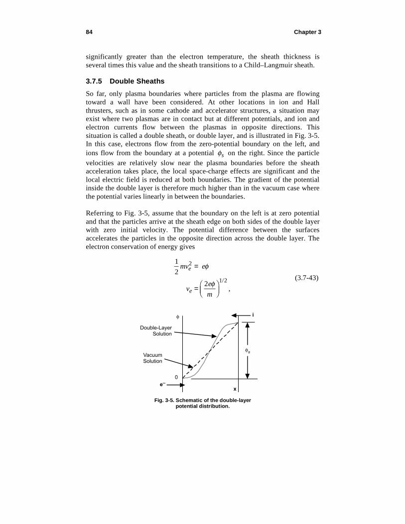
84 Chapter 3

��$��%��

&�'��

�

φ�

�

�−�

φ

Fig. 3-5. Schematic of the double-layer potential distribution.

significantly greater than the electron temperature, the sheath thickness is

several times this value and the sheath transitions to a Child–Langmuir sheath.

3.7.5 Double Sheaths

So far, only plasma boundaries where particles from the plasma are flowing

toward a wall have been considered. At other locations in ion and Hall

thrusters, such as in some cathode and accelerator structures, a situation may

exist where two plasmas are in contact but at different potentials, and ion and

electron currents flow between the plasmas in opposite directions. This

situation is called a double sheath, or double layer, and is illustrated in Fig. 3-5.

In this case, electrons flow from the zero-potential boundary on the left, and

ions flow from the boundary at a potential s on the right. Since the particle

velocities are relatively slow near the plasma boundaries before the sheath

acceleration takes place, the local space-charge effects are significant and the

local electric field is reduced at both boundaries. The gradient of the potential

inside the double layer is therefore much higher than in the vacuum case where

the potential varies linearly in between the boundaries.

Referring to Fig. 3-5, assume that the boundary on the left is at zero potential

and that the particles arrive at the sheath edge on both sides of the double layer

with zero initial velocity. The potential difference between the surfaces

accelerates the particles in the opposite direction across the double layer. The

electron conservation of energy gives

1

2mve

2= e

ve =2e

m

1/2

,

(3.7-43)


and the ion energy conservation gives

1

2Mvi

2= e s –( )

vi =2e

M s –( )1/2

.

(3.7-44)

The charge density in Eq. (3.2-5) can be written

= i + e

=Ji

vi–

Je

ve=

Ji

s –

M

2e –

Je m

2e. (3.7-45)

Poisson’s equation can then be written in one dimension as

dE

dx=

o=

Ji

o s –

M

2e –

Je

o

m

2e. (3.7-46)

Integrating once gives

o

2E2

= 2JiM

2e s – s –( )1/2 – 2Je

m

2e1/2 . (3.7-47)

For space-charge-limited current flow, the electric field at the right-hand

boundary (the edge of the plasma) is zero and the potential is = s . Putting

that into Eq. (3.7-47) and solving for the current density gives

Je =M

m Ji . (3.7-48)

If the area of the two plasmas in contact with each other is the same, the

electron current crossing the double layer is the square root of the mass ratio

times the ion current crossing the layer. This situation is called the Langmuir

condition (1929) and describes the space-charge-limited flow of ions and

electrons between two plasmas or between a plasma and an electron emitter.

For finite initial velocities, Eq. (3.7-48) was corrected by Andrews and Allen

[13] to give

Je = M

m Ji , (3.7-49)

86 Chapter 3

where is a constant that varies from 0.8 to 0.2 for Te /Ti changing from 2 to

about 20. For typical thruster plasmas where Te /Ti 10 , k is about 0.5.

While the presence of free-standing double layers in the plasma volume in

thrusters is often debated, the sheath at a thermionic cathode surface certainly

satisfies the criteria of counter-streaming ion and electron currents and can be

viewed as a double layer. In this case, Eq. (3.7-49) describes the space-charge-

limited current density that a plasma can accept from an electron-emitting

cathode surface. This is useful in that the maximum current density that can be

drawn from a cathode can be evaluated if the plasma parameters at the sheath

edge in contact with the cathode are known (such that Ji can be evaluated from

the Bohm current), without requiring that the actual sheath thickness be known.

Finally, there are several conditions for the formation of the classic double

layer described here. In order to achieve a potential difference between the

plasmas that is large compared to the local electron temperature, charge

separation must occur in the layer. This, of course, violates quasi-neutrality

locally. The current flow across the layer is space-charge limited, which means

that the electric field is essentially zero at both boundaries. Finally, the flow

through the layer discussed here is collisionless. Collisions cause resistive

voltage drops where current is flowing, which can easily be confused with the

potential difference across a double layer.

3.7.6 Summary of Sheath Effects

It is worthwhile to summarize here some of the important equations in this

section related to sheaths because these will be very useful later in describing

thruster performance. These equations were derived in the sections above, and

alternative derivations can be found in [1–3].

The current density of ions entering the sheath at the edge of the plasma is

given by

Ji = 0.6 nevi1

2ne

kTe

M, (3.7-50)

where n is the plasma density at the start of the pre-sheath far from the

boundary, which was considered to be the center of the plasma by Langmuir for

his collisionless plasmas. The convention of approximating the coefficient 0.6

as 1/2 was made by Bohm in defining what is now called the “Bohm current.”


If there is no net current to the boundary, the ion and electron currents must be

equal. The Bohm current of ions through the sheath is given by the current

density in Eq. (3.7-50) times the wall area A:

Ii =1

2ni e

kTe

MA . (3.7-51)

The electron current through the sheath is the random electron flux times the

Boltzmann factor:

Ie =1

4

8kTe

m ne eA exp –

e

kTe, (3.7-52)

where the potential is by convention a positive number in this formulation.

Equating the total ion and electron currents ( Ii = Ie ), assuming quasi-neutrality

in the plasma ( ni = ne ), and solving for the potential gives

=kTe

eln

2M

m. (3.7-53)

This is the potential at which the plasma will self-bias in order to have zero net

current to the walls and thereby conserve charge and is often called the floating

potential. Note that the floating potential is negative relative to the plasma

potential.

For sheath potentials less than the electron temperature, the sheath thickness is

given by the Debye length:

D = okTe

noe2. (3.7-54)

For sheath potentials greater than the electron temperature ( e > kTe ), a pre-

sheath forms to accelerate the ions into the sheath to avoid any inflection in the

potential at the sheath edge. The collisionless pre-sheath has a potential

difference from the center of the plasma to the sheath edge of Te / 2 and a

density decrease from the center of the plasma to the sheath edge of 0.61 no .

The Te / 2 potential difference accelerates the ions to the Bohm velocity:

vBohm = vB =kTe

M. (3.7-55)

88 Chapter 3

The sheath thickness at the wall depends on the plasma parameters and the

potential difference between the plasma and the wall, and is found from the

solution of Eq. (3.7-42).

For the case of sheath potentials that are large compared to the electron

temperature ( e >> kTe ), the current density through the sheath is described by

the Child–Langmuir equation:

Ji =4eo

9

2e

M

1/2 3/2

d2. (3.7-56)

Finally, for the case of double sheaths where ion and electrons are

counterstreaming across the boundary between two plasmas, the relationship

between the two currents is

Je = M

m Ji . (3.7-57)

If one boundary of the double layer is the sheath edge at a thermionic cathode,

Eq. (3.7-51) can be used for the Bohm current to the opposite boundary to give

the maximum emission current density as

Je =2

ni ekTem

1

4ne e

kTem

. (3.7-58)

This is the maximum electron current density that can be accepted by a plasma

due to space-charge effects at the cathode double sheath. For example, the

maximum space-charge-limited cathode emission current into a xenon plasma

with a density of 1018

m–3

and an electron temperature of 5 eV is about

3.8 A/cm2.

These summary equations are commonly seen in the literature on the design

and analysis of ion sources, plasma processing sources, and, of course, many

electric propulsion thrusters.

References

[1] F. F. Chen, Introduction to Plasma Physics and Controlled Fusion, vol. 1,

New York: Plenum Press, 1984.

[2] M. Lieberman and A. Lichtenberg, Principles of Plasma Discharges and

Materials Processing, New York: John Wiley and Sons, 1994.


[3] R. J. Goldston and P. H. Rutherford, Introduction to Plasma Physics,

London: Institute of Physics Publishing, 1995.

[4] A. T. Forrester, Large Ion Beams, New York: John Wiley and Sons, 1988.

[5] D. L. Book, NRL Plasma Formulary, Washington, D.C.: Naval Research

Laboratory, 1987.

[6] E. A. Mason and E. W. McDaniel, Transport Properties of Ions in Gases,

New York: John Wiley and Sons, 1988.

[7] J. S. Miller, S. H. Pullins, D. J. Levandier, Y. Chiu, and R. A. Dressler,

“Xenon Charge Exchange Cross Sections for Electrostatic Thruster

Models,” Journal of Applied Physics, vol. 91, no. 3, pp. 984–991, 2002.

[8] I. Katz, J. Anderson, J. Polk and J. Brophy, “One Dimensional Hollow

Cathode Model,” Journal of Propulsion and Power, vol. 19, no. 4,

pp. 595–600, 2003.

[9] L. Spitzer, Jr., Physics of Fully Ionized Gases, New York: Interscience,

pp. 127–135, 1962.

[10] D. Bohm, Chapter 1, The Characteristics of Electric Discharges in

Magnetic Fields, edited by A. Guthrie and R. Wakerling, New York:

McGraw-Hill, pp. 1–76, 1949.

[11] C. D. Child, “Discharge from Hot CaO,” Physical Review, vol. 32, p. 492,

1911.

[12] I. Langmuir, “The Effect of Space Charge and Residual Gases on

Thermionic Currents in High Vacuum,” Physical Review, vol. 2, p. 450,

1913.

[13] J. G. Andrews and J. E. Allen, “Theory of a Double Sheath Between Two

Plasmas,” Proceedings of the Royal Society of London, series A, vol. 320,

pp. 459–472, 1971.

Homework Problems

1. Show that Eq. (3.2-7) becomes E = – – A/ t when B is varying with

time, where A is the “vector potential.” How are A and B related?

2. Derive Eq. (3.3-21) for the force on a particle in a magnetic mirror.

3. Show that the magnetic moment is invariant and derive Eq. (3.3-23).

4. Derive the expression for ion acoustic velocity in Eq. (3.5-26).

90 Chapter 3

5. Answer the following question that might be brought up by a student

working in the lab: “In a plasma discharge set up in my vacuum chamber

the other day, I measured an increase in the plasma potential with an

electrostatic probe. How do I know if it’s a double layer or just a potential

gradient within which the ionized gas is quasi-neutral?”

6. Derive Eq. (3.6-9) for the penetration distance of neutral particles in a

plasma.

7. Derive the expression for Ohm’s law for partially ionized plasmas,

Eq. (3.6-20).

8. Derive Eq. (3.6-81) for the transverse ambipolar ion velocity across

magnetic field lines.

9. Derive the Bohm sheath criteria including the presence of double ions.

10. Derive an expression equivalent to the Child–Langmuir law for the

condition where the initial ion velocity entering the sheath is not neglected

(ions have an initial velocity vo at the sheath edge at z = 0 ).

11. A 2-mm by 2-mm square probe is immersed in a 3 eV xenon plasma.

a. If the probe collects 1 mA of ion current, what is the plasma density?

(Hint: the probe has two sides and is considered infinitely thin.)

b. What is the floating potential?

c. What is the probe current collected at the plasma potential?

12. A 2-mm-diameter cylindrical probe 5 mm long in a xenon plasma with

Te = 3 eV collects 1 mA of ion saturation current.

a. What is the average plasma density?

b. How much electron current is collected if the probe is biased to the

plasma potential?

c. Why is this electron current the same as the solution to Problem 11.c

when the plasma densities are so different?

13. An electron emitter capable of emitting up to 10 A/cm2 is in contact with an

Xe+ plasma with an electron temperature of 2 eV. Plot the emission current

density versus plasma density over the range from 1010

to 1013

cm–3

. At

what density does the emission become thermally limited (the maximum

current density that the electron emitter can emit)?

basic plasma physics - descanso

Documents