basic computability theory - universiteit utrechtooste110/syllabi/compthmoeder.pdf · basic...
TRANSCRIPT

Basic Computability Theory
Jaap van Oosten
Department of Mathematics
Utrecht University
1993, revised 2013

ii
Introduction
The subject of this course is the theory of computable or recursive functions. Computability Theoryand Recursion Theory are two names for it; the former being more popular nowadays.
0.1 Why Computability Theory?
The two most important contributions Logic has made to Mathematics, are formal definitions ofproof and of algorithmic computation.
How useful is this? Mathematicians are trained in understanding and constructing proofs fromtheir first steps in the subject, and surely they can recognize a valid proof when they see one;likewise, algorithms have been an essential part of Mathematics for as long as it exists, and atthe most elementary levels (think of long division, or Euclid’s algorithm for the greatest commondivisor function). So why do we need a formal definition here?
The main use is twofold. Firstly, a formal definition of proof (or algorithm) leads to an analysisof proofs (programs) in elementary reasoning steps (computation steps), thereby opening up thepossibility of numerical classification of proofs (programs)1. In Proof Theory, proofs are assignedordinal numbers, and theorems are classified according to the complexity of the proofs they need.In Complexity Theory, programs are analyzed according to the number of elementary computationsteps they require (as a function of the input), and programming problems are classified in termsof these complexity functions.
Secondly, a formal definition is needed once one wishes to explore the boundaries of the topic:what can be proved at all? Which kind of problems can be settled by an algorithm? It is thisaspect that we will focus on in this course.
There are, of course, other reasons for studying a formal definition of algorithms and compu-tations: for example, the definition leads to generalizations (for example, where computation isdone not on numbers, but on objects of higher type such as functions, or functionals (see, e.g.,[33]); or where basic properties of algorithms are taken as axioms for an abstract theory, such asin the study of Partial Combinatory Algebras (see chapter 1 of [41])).
After settling on a definition of ‘algorithm’ (a program in an extremely simple language), wedefine what we call a ‘computable function’ (a function whose values can be computed using analgorithm). This leads to an indexing of computable functions, and we study the structure of thisindexed collection. We learn techniques for proving that for certain problems there cannot exist analgorithm. A further topic is the classification of problems according to ‘relative computability’:can I solve problem A on the assumption that I can solve B? Suppose an ‘oracle’ tells me how tosolve B, can I then construct an algorithm for A?
In the meantime, we shall also learn about a class of functions (the primitive recursive functionswhich are of importance in other areas of Logic, such as the analysis of systems of Arithmetic (andGodel’s Incompleteness Theorems).
1Contrary to a widely held misconception, the aim of Logic is not to tell people how they should reason; thepurpose of Logic is to understand how correct reasoning can be analyzed
iii

iv
0.2 A bit of early history
I have taken most of this section from the paper [9], which I highly recommend.Calculation by a machine was thought of by the universal genius Gottfried Wilhelm Leibniz
(1646–1716), who conceived the Calculus ratiocinator which is seen by some as a precursor toTuring’s universal machine. But the first one who not only thought of such calculation but actuallyconstructed calculating machines was Charles Babbage (1791–1871), an English mathematicianand engineer. Babbage did not publish his ideas; this was done by Luigi Menabrea (1809–1896)2,whose French text was translated, with notes, by Lady Ada Augusta Lovelace3 (1815–1852).
It is, however, perhaps ironic that the theoretical work which immediately preceded the con-struction of the modern computer, focused not on what a machine can calculate, but on what ahuman being (a mathematician, following a precise routine) can calculate4. Although Babbagecame quite close to formulating the notion of a computable function in the later sense of Church-Kleene-Turing-Post, it is argued in [9] that it may have been because of the focus on “hardware”that his work was not very influential5.
Instead, another stream of thought played an important role. Mathematics became moreand more the study of abstract axiomatic systems in the 19th century, and with axiom systemscome questions such as: is the axiom system consistent (i.e., free of contradiction)? How canone determine the consequences of the axioms? No one was more influential in stressing theimportance of such questions than David Hilbert (1862-1943). Hilbert was one of the greatestmathematicians of his time. He was a very modern mathematician; he embraced wholeheartedlyCantor’s theory of sets with its higher infinities and transfinite recursions6. In 1900, Hilbertaddressed the International Congress of Mathematicians in Paris and proposed 23 problems forthe new century. Some are about Logic, for example:
1 Settle the Continuum Hypothesis
2 Prove that the axioms of arithmetic are consistent
and some have been resolved using techniques from Logic, such as
10 Find an algorithm to determine whether a polynomial equation with integer coefficients hasa solution in the integers
17 Prove that a positive definite rational function is a sum of squares
We see, Hilbert often asked for an “algorithm”. Another problem he posed, came to be known(also in English-language texts) as the “Entscheidungsproblem”: find an algorithm to decidewhether a given sentence of first-order logic is valid.
There were also other, foundational issues which influenced Hilbert. Some mathematicians(like Kronecker and Brouwer) openly doubted the existence of infinite objects in Mathematicsand adopted the philosophical stance of Finitism (Brouwer called his philosophy Intuitionism).Hilbert’s plan of attack on these positions was imaginative: he created Proof Theory7. His ideawas as follows: let us analyze proofs, which are finite objects; and in analyzing proofs let us restrictourselves to methods that are completely unproblematic from the finitist point of view. The kindof methods permitted is laid out in [12]8. And then, using these unproblematic methods, let usprove that classical mathematics is consistent. This became known as Hilbert’s Program. When
2Apart from being a mathematician, Menabrea was also a general who played an important role in the Unificationof Italy; after conflicts with Garibaldi, he became Prime Minister
3A daughter of the poet Byron. The programming language Ada is named after her. Babbage named her “theEnchantress of Numbers”
4In Turing’s seminal paper [40], the word “computer” refers to a human5As [9] convincingly argues, Turing was probably not aware of Babbage’s work when he wrote [40]6He coined the phrase Cantor’s Paradise7Beweistheorie8Some people have concluded from the discussion there of the “finitary point of view” that Hilbert was a finitist;
in my opinion, he was certainly not
0.3. SOME LATER DEVELOPMENTS v
the finitist mathematician had to work with functions (which are usually infinite), these wouldhave to have a finite presentation, that is: an algorithm. So, Hilbert became interested in thestudy of functions which can be produced by algorithms, and togethr with Ackermann ([11]) hedeveloped the class of functions that Godel later would call “recursive”, and Kleene “primitiverecursive”, the terminology still in use today.
There is an enormous literature on Hilbert’s discussion with the Finitists/Intuitionists, a dis-cussion which came to be referred to as Grundlagenstreit (Battle of Foundations). For a bit ofintroduction, read Chapter III, section 1, of [37]. Also see [36, 7].
Godel proved that if one took the “finitary point of view” to mean “first-order arithmetic”, thenHilbert’s program was bound to fail since first-order arithmetic cannot prove its own consistency,let alone that of Mathematics. But still, Hilbert’s program and Hilbert’s continued interest infoundational matters was extremely fruitful.
In the meantime, in the 1920’s, the American mathematician Alonzo Church (1903–1995) haddeveloped the Lambda Calculus (see [2] for an introduction) as a formalism for doing Mathematics.
In 1936, four papers appeared, each proposing a definition of “algorithmically computable”:[5, 40, 19, 29]. Church proposed for “algorithmically computable”: representable by a λ-term.Kleene proposed a definition in the form of schemes for constructing functions. Post’s paper isvery short and poor on details. The paper by Turing stands out in readability and novelty ofapproach; highly recommended reading! Read [14] for an account of Alan Turing’s dramatic life.
It was soon realized that the four approaches all defined the same class of functions. Churchand Turing moreover noted that with the new, precise definition of algorithmically computableand Godel’s results, one could settle the Entscheidungsproblem in the negative: there cannot existsuch an algorithm.
0.3 Some later developments
Of the four pioneers in 1936 (Church, Kleene, Turing and Post), only Kleene and Post developedthe theory of “recursive functions” (as they were now called) further. The most important wasStephen Cole Kleene (1909–1994), who shaped much of it single-handedly. In particular, hediscovered the Recursion Theorem (see theorem 2.4.3 below).
Here, I just mention a number of topics that were investigated.
Definability Recursion theory studies definable sets , subsets of Nk for some k which havea logical description. By a technique called many-one reducibility such sets can be classifiedin an Arithmetical Hierarchy. We shall see that in these notes. The classification of arith-metically definable sets is carried further in the study of the Analytical Hierarchy, and alsoin the field of Descriptive Set Theory.
Subrecursion There is a hierarchy, indexed by the countable ordinals, of classes of com-putable functions. In this hierarchy, the primitive recursive functions arise at level ω and thefunctions which are provably total in Peano Arithmetic (see section 2.1.2 for an explanationof this notion) arise at level ε0. For an exposition of this area, see [32].
Degrees of Unsolvabiity We can ask ourselves which problems can be effectively solvedprovided a given problem is solved for us, in whatever way (Turing used the word “oracle”).This leads to the important notion of “Turing reducibility”, which we shall also meet in thiscourse. This relation divides the subsets of N into equivalence classes, called “Turing de-grees”. The degrees form an upper semilattice, which is vast and very complicated. Alreadyfor degrees of ‘recursively enumerable sets’ (the lowest class of non-computable sets) thereis a lot of theory; see the excellent books [38, 13].
Recursion in Higher Types When is a function on functions, that is, a functional oftype 1, to be called computable? And a function on functionals of type 1, and so forth?Kleene started thinking about this in the 1950’s and produced a number of deep papers([20, 21] among others) about it. Apart from the already mentioned book by Sanchis, an
vi
introduction to this area can be found in [17]. The study of recursive functionals of highertype was revived when theoretical computer scientists studied the programming languagePCF and “fully abstract” models for it.
Realizability Kleene also observed, that the theory of computable functions can be usedto give a model for a form of reasoning (advocated by Brouwer) in which the ‘principle ofexcluded third’, A∨¬A, need not be valid. The basic paper is [18]. Realizability, originally aproof-theoretic tool, turned into an independent field of study with M. Hyland’s paper [15],which connects the world of partial recursive functions with Topos Theory. See also [41].
Recursive Mathematics This is the study of familiar mathematical structures (groups,rings, lattices, CW-complexes, real analysis) from the point of computability. For analysis,see [30]
Hilbert 10 and Number Theory In 1970, Yuri Matiyasevich used notions of Computabil-ity Theory to show that Hilbert’s 10-th Problem cannot be solved: there is no algorithmwhich decides, for a given polynomial equation with integer coefficients, whether it has asolution in the integers. This result was extremely important and has applications through-out Logic, for example in the theory of Models of Peano Arithmetic ([16]). But even moreinterestingly, number theorists have been thinking about replacing Z by other number ringsand number fields (for example, Q). Some introduction can be found in the very readablepaper [28].
0.4 What is in these notes?
These notes consist of 6 chapters.
The first chapter treats our preferred model of computation, Register Machines. We define thenotion of an (RM)-computable function and prove some closure properties of these functions.
Chapter 2 starts with the theory of primitive recursive functions. We develop coding of sequences,then coding of programs for the Register Machine; the Kleene T -predicate; Smn-Theorem andRecursion Theorem.
Chapter 3 introduces unsolvable problems and then moves on to recursively enumerable sets. Wegive the “Kleene tree”. We treat extensional sets and prove the Myhill-Shepherdson, Rice-Shapiroand Kreisel-Lacombe-Shoenfield Theorems. Examples of r.e. sets outside Recursion Theory aregiven.
Chapter 4 deals with many-one reducibility and the Arithmetical Hierarchy. We practice someexact classifications. A final section treats the equivalence: m-complete ⇔ creative, via Myhill’sIsomorphism Theorem. Post’s construction of a simple set is given.
Chapter 5 gives the concept of computability relative to an oracle. The jump is defined and itsbasic properties are derived. We prove a theorem by Friedberg saying that the jump operation issurjective on the degrees above the junp of the empty set.
Chapter 6 provides a glimpse at the Analytical Hierarchy. Starting with recursive functionals, wedefine the notion Σ1
n-set. We show that the collection of indices of recursive well-founded trees ism-complete in Π1
1. We prove that the set of (codes of) true arithmetical sentences is ∆11. Without
proof, we mention the “Kleene tree” analogue for ∆11 and the Suslin-Kleene Theorem.
0.5 Literature
Authoritative monographs on the general theory of computable functions are [31] and [26, 27]. Anoutline is [35]. Good introductory text books are [6] and [3].
0.6. ACKNOWLEDGEMENTS vii
0.6 Acknowledgements
I learned Recursion Theory from Dick de Jongh, who was a student of Kleene. De Jongh had hisown notes, but also used a set of lecture notes prepared by Robin Grayson. My lecture notes grewout of these notes by De Jongh and Grayson, but gradually I reworked the material and added toit.
viii
Contents
0.1 Why Computability Theory? . . . . . . . . . . . . . . . . . . . . . . . . . . . . . . iii
0.2 A bit of early history . . . . . . . . . . . . . . . . . . . . . . . . . . . . . . . . . . . iv
0.3 Some later developments . . . . . . . . . . . . . . . . . . . . . . . . . . . . . . . . . v
0.4 What is in these notes? . . . . . . . . . . . . . . . . . . . . . . . . . . . . . . . . . vi
0.5 Literature . . . . . . . . . . . . . . . . . . . . . . . . . . . . . . . . . . . . . . . . . vi
0.6 Acknowledgements . . . . . . . . . . . . . . . . . . . . . . . . . . . . . . . . . . . . vii
1 Register Machines and Computable Functions 1
1.1 Register Machines . . . . . . . . . . . . . . . . . . . . . . . . . . . . . . . . . . . . 1
1.2 Partial computable functions . . . . . . . . . . . . . . . . . . . . . . . . . . . . . . 3
2 Recursive Functions 7
2.1 Primitive recursive functions and relations . . . . . . . . . . . . . . . . . . . . . . . 7
2.1.1 Coding of pairs and tuples . . . . . . . . . . . . . . . . . . . . . . . . . . . . 10
2.1.2 A Logical Characterization of the Primitive Recursive Functions . . . . . . 16
2.2 Partial recursive functions . . . . . . . . . . . . . . . . . . . . . . . . . . . . . . . . 16
2.3 Coding of RM-programs and the equality Computable = Recursive . . . . . . . . . 17
2.4 Smn-Theorem and Recursion Theorem . . . . . . . . . . . . . . . . . . . . . . . . . 20
3 Undecidability and Recursively Enumerable Sets 25
3.1 Solvable Problems . . . . . . . . . . . . . . . . . . . . . . . . . . . . . . . . . . . . 25
3.2 Recursively Enumerable Sets . . . . . . . . . . . . . . . . . . . . . . . . . . . . . . 28
3.2.1 The Kleene Tree . . . . . . . . . . . . . . . . . . . . . . . . . . . . . . . . . 31
3.3 Extensional r.e. sets and effective operations . . . . . . . . . . . . . . . . . . . . . . 33
3.3.1 Theorems of Myhill-Shepherdson, Rice-Shapiro and Kreisel-Lacombe-Shoenfield 34
3.4 Strict r.e. sets in Mathematics and Logic . . . . . . . . . . . . . . . . . . . . . . . . 39
3.4.1 Hilbert’s Tenth Problem . . . . . . . . . . . . . . . . . . . . . . . . . . . . . 39
3.4.2 Word Problems: Groups . . . . . . . . . . . . . . . . . . . . . . . . . . . . . 39
3.4.3 Theorems by Church and Trakhtenbrot . . . . . . . . . . . . . . . . . . . . 40
4 Reduction and Classification 43
4.1 Many-one reducibility . . . . . . . . . . . . . . . . . . . . . . . . . . . . . . . . . . 43
4.2 The Arithmetical Hierarchy . . . . . . . . . . . . . . . . . . . . . . . . . . . . . . . 45
4.2.1 Some exact classifications . . . . . . . . . . . . . . . . . . . . . . . . . . . . 50
4.3 R.e. sets again: recursive, m-complete, and in-between . . . . . . . . . . . . . . . . 52
4.3.1 Extensional r.e. sets . . . . . . . . . . . . . . . . . . . . . . . . . . . . . . . 53
4.3.2 m-Complete r.e. sets . . . . . . . . . . . . . . . . . . . . . . . . . . . . . . . 53
4.3.3 Simple r.e. sets: neither recursive, nor m-complete . . . . . . . . . . . . . . 56
4.3.4 Non-Arithmetical Sets; Tarski’s Theorem . . . . . . . . . . . . . . . . . . . 56
ix
x CONTENTS
5 Relative Computability and Turing Reducibility 595.1 Functions partial recursive in F . . . . . . . . . . . . . . . . . . . . . . . . . . . . . 595.2 Sets r.e. in F ; the jump operation . . . . . . . . . . . . . . . . . . . . . . . . . . . . 615.3 The Relativized Arithmetical Hierrarchy . . . . . . . . . . . . . . . . . . . . . . . . 63
6 A Glimpse Beyond the Arithmetical Hierarchy 656.1 Partial Recursive Functionals . . . . . . . . . . . . . . . . . . . . . . . . . . . . . . 656.2 The Analytical Hierarchy . . . . . . . . . . . . . . . . . . . . . . . . . . . . . . . . 676.3 Well-founded trees: an m-complete Π1
1-set of numbers . . . . . . . . . . . . . . . . 686.4 Hyperarithmetical Sets and Functions . . . . . . . . . . . . . . . . . . . . . . . . . 70
Bibliography 72
Index 74
Chapter 1
Register Machines and
Computable Functions
In his pioneering paper [40], Alan Turing set out to isolate the essential features of a calculation,done by a human (the “computer”), who may use pen and paper, and who is working followinga definite method. Turing argues that at any given moment of the calculation, the mind of the“computer” can be in only one of a finite collection of states, and that in each state, given theintermediate results thus far obtained, the next calculation step is completely determined.
A mathematical formulation of this is the Turing machine. Turing machines still have aprominent place in text books on Computability Theory and Complexity Theory, but for thiscourse we prefer a concept which is closed to present-day programming on an actual computer: theRegister Machine, developed in the 1960s. There are many names associated with this development(Cook, Elgot, Hartmanis, Lambek, Melzak, Minsky, Reckhow, Robinson) but the most cited isthat of Marvin Lee Minsky (born 1927).
The notions of Turing Machine and Register Machine give rise to the same notion of ‘com-putable function’.
1.1 Register Machines
We picture ourselves a machine, the Register Machine, which has an infinite, numbered collectionof memory storage places or registers R1, R2, . . ., each of which can store a natural number ofarbitrary size. The number stored in register Ri is denoted ri.
Furthermore the Register Machine modifies the contents of its registers in response to com-mands in a program. Such a program is a finite list of commands which all have one of the followingtwo forms:
the command r+i ⇒ n (which is read as: “add 1 to ri, and move to the n-th command”)
the command r−i ⇒ n,m (which is read as: “if ri > 0, subtract 1 from ri and move to then-th command; otherwise, move to the m-th command”)
It may happen that the ‘move to the n-th command’ is impossible to execute because there is non-th command; in that case, the machine stops.
Let us, before formulating a more mathematical definition, see a few simple programs and theirintended effects. In these examples, we put numbers before the commands for clarity; these arenot part of the programming language.
Example 1.1.1 a) 1 r+i ⇒ 2
The machine adds 1 to ri, and stops.
1

2 CHAPTER 1. REGISTER MACHINES AND COMPUTABLE FUNCTIONS
b) 1 r+i ⇒ 1
The machine keeps on adding 1 to ri.
c) 1 r−i ⇒ 1, 2
The machine empties register Ri, and stops.
d)1 r−i ⇒ 2, 32 r+j ⇒ 1
The machine carries the content of Ri over to Rj .
e)
1 r−i ⇒ 2, 42 r+j ⇒ 3
3 r+k ⇒ 1
The machine carries the content of Ri simultaneously over to Rj and Rk.
Exercise 1 An alternative notion of machine, the Unlimited Register Machine of [6] has 4 typesof commands:
1) The command Z(i) is read as: “empty Ri, and move to the next command”
2) The command S(i) is read as: “add 1 to ri, and move to the next command”
3) The command T (m,n) is read as: “replace rn by rm and move to the next command”
4) The command J(m,n, q) is read as: “if rm = rn, move to the q-th command; otherwise,move to the next command”
For each of these commands, write a short RM-program which has the same effect.
Clearly, the Register Machine is not really a mathematical object. A program, on the other hand,can be seen as a finite list of which each item is either an ordered pair or an ordered triple ofpositive integers.
We now define the notion of a computation of the RM with input a1, . . . , ak and program P .
Definition 1.1.2 Let P be a program for the RM, and a1, . . . , ak a list of natural numbers. Acomputation of the Register Machine with program P and input a1, . . . , ak is a finite or infinite listof l+ 1-tuples
(ni, ri1, . . . , r
il )i≥1
with the following properties:
a) l ≥ k, and (n1, r11 , . . . , r
1l ) = (1, a1, . . . , ak, 0, . . . , 0)
b) If ni = m then exactly one of the following three situations occurs:
b1 The program P does not have an m-th command, and the i-th tuple is the last item ofthe list (so the computation is finite);
b2 The m-th command of P is r+j ⇒ u, j ≤ l, ni+1 = u and
(ri+11 , . . . , ri+1
l ) = (ri1, . . . , rij−1, r
ij + 1, rij+1, . . . , r
il)
b3 The m-th command of P is r−j ⇒ u, v, j ≤ l, and now either rij > 0 and
(ni+1, ri+11 , . . . , ri+1
l ) = (u, ri1, . . . , rij − 1, . . . , ril )
or rij = 0 and
(ni+1, ri+11 , . . . , ri+1
l ) = (v, ri1, . . . , ril )

1.2. PARTIAL COMPUTABLE FUNCTIONS 3
If a computation is finite, with last element (nK , rK1 , . . . , r
Kl ), then the number rK1 is the output
or result of the computation.
Remark 1.1.3 Clearly, if (ni, ri1, . . . , r
il )i≥1 is a computation with P and input a1, . . . , ak, and
l′ ≥ l, then the list of l′ + 1-tuples
(ni, ri1, . . . , r
il , 0, . . . , 0)i≥1
is also a computation with P and input a1, . . . , ak. But once l is fixed, computations are unique:the RM is deterministic.
A program can be the empty list. Clearly, the list consisting of the single l + 1-tuple
(1, a1, . . . , ak, 0, . . . , 0)
is the unique computation with the empty program and input a1, . . . , ak.
Definition 1.1.4 (Composition of programs) If P and Q are programs, there is a composi-tion PQ, defined as follows. Suppose P has k commands. First modify P to P ′ by replacing everycommand number n > k by k+1 (so r+i ⇒ n becomes r+i ⇒ k+1, etc.). Then modify Q to obtainQ′′ by replacing each command number m in Q by k+m (so r+i ⇒ m becomes r+i ⇒ k+m, etc.)
The program PQ is now the list of commands P ′ followed by the list of commands Q′′.
Exercise 2 Show that the operation of composition on programs is associative. Show also thatif Q is the empty program, QP = P for any program P . What about PQ?
Notation for computations. We write
a1 a2 · · · ak⇓ P
b1 b2 · · · bm
or
~a⇓ P~b
when there is a finite computation (ni, ri1, . . . , r
il )Ki=1 with program P and input a1, . . . , ak, such
that (rK1 , . . . , rKl ) = (b1, . . . , bm, 0, . . . , 0).
Clearly,
if
~a⇓ P~b
and
~b⇓ Q~c
then~a⇓ PQ~c
1.2 Partial computable functions
A function f : A → N with A ⊆ Nk is called a partial function of k arguments, or a k-ary partialfunction. For k = 1, 2, 3 we say unary, binary, ternary, respectively. The set A is the domain off , written dom(f). If dom(f) = Nk then f is called total; for us, a total function is a special caseof a partial function.
Definition 1.2.1 Let f be a k-ary partial function. Then f is called RM-computable or com-putable for short, if there is a program P such that for every k-tuple a1, . . . , ak of natural numberswe have:
i) if ~a ∈ dom(f) then there is a finite computation (ni, ri1, . . . , r
il )Ki=1 with P and input ~a, such
that rK1 = f(~a);
ii) if ~a 6∈ dom(f) then there is no finite computation with P and input ~a.
We say that the program P computes f .

4 CHAPTER 1. REGISTER MACHINES AND COMPUTABLE FUNCTIONS
Note, that it does not follow from definition 1.2.1 that if f is computable, then the restriction off to a smaller domain is also computable!
Exercise 3 Suppose f is a computable function of k variables. Show that there is a program Pwhich computes f in such a way that for every ~a ∈ dom(f),
~a⇓ P
f(~a)~a
We derive some closure properties of the class of computable functions.
Definition 1.2.2 Suppose g1, . . . , gl are partial k-ary functions and h is partial l-ary. The partialk-ary function f with domain
{~x ∈ Nk | ~x ∈l⋂
i=1
dom(gi) and (g1(~x), . . . , gl(~x)) ∈ dom(h)}
and defined by f(~x) = h(g1(~x, . . . , gl(~x)) is said to be defined from g1, . . . , gl, h by composition.
Definition 1.2.3 Suppose g is a partial k-ary function and h is partial k + 2-ary. Let f be theleast partial k + 1-ary function with the properties:
i) if (x1, . . . , xk) ∈ dom(g) then (0, x1, . . . , xk) ∈ dom(f), and
f(0, x1, . . . , xk) = g(x1, . . . , xk)
ii) if (y, x1, . . . , xk) ∈ dom(f) and (y, f(y, x1, . . . , xk), x1, . . . , xk) ∈ dom(h) then (y+1, x1, . . . , xk) ∈dom(f) and
f(y + 1, x1, . . . , xk) = h(y, f(y, x1, . . . , xk), x1, . . . , xk)
(Here, partial functions are seen as relations; so f is the intersection of all partial functionssatisfying i) and ii))Then f is said to be defined from g and h by primitive recursion.
Exercise 4 Suppose f is defined by primitive recursion from g and h as above. Show that if(y, ~x) ∈ dom(f) then for all w < y, (w, ~x) ∈ dom(f).
Remark 1.2.4 In definition 1.2.3 we do not exclude the case k = 0; a ‘partial 0-ary function’is either a number, or undefined. Clearly, if g is the undefined partial 0-ary function and f isdefined by primitive recursion from g and h, dom(f) = ∅ (f is the empty function). In the casethat g = n we have: f(0) = n, and if y ∈ dom(f) and (y, f(y)) ∈ dom(h), then y + 1 ∈ dom(f)and f(y + 1) = h(y, f(y)).
Definition 1.2.5 Suppose g is partial k + 1-ary. Let f be the partial k-ary function such that(x1, . . . , xk) ∈ dom(f) precisely if there is a number y such that the k + 1-tuples (0, ~x), . . . , (y, ~x)all belong to dom(g) and g(y, ~x) = 0; and f(~x) is the least such y, in that case. Then f is said tobe defined from g by minimalization.
Theorem 1.2.6 The class of partial computable functions is closed under definition by composi-tion, primitive recursion and minimalization.
Proof. Recall the result of exercise 3: if f is partial computable then there is a program P whichcomputes f and is such that for all ~a ∈ dom(f),
~a⇓ P
f(~a)~a
1.2. PARTIAL COMPUTABLE FUNCTIONS 5
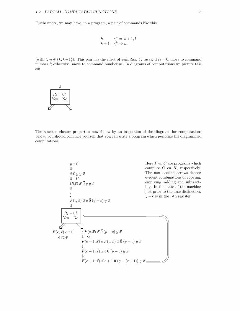
Furthermore, we may have, in a program, a pair of commands like this:
k r−i ⇒ k + 1, lk + 1 r+i ⇒ m
(with l,m 6∈ {k, k+1}). This pair has the effect of definition by cases: if ri = 0, move to commandnumber l; otherwise, move to command number m. In diagrams of computations we picture thisas:
Ri = 0?Yes No
⇓
The asserted closure properties now follow by an inspection of the diagrams for computationsbelow; you should convince yourself that you can write a program which performs the diagrammedcomputations.
y ~x ~0⇓
~x ~0 y y ~x⇓ P
G(~x) ~x ~0 y y ~x⇓...
F (c, ~x) ~x c ~0 (y − c) y ~x
Ri = 0?Yes No
⇓
F (c, ~x) c ~x ~0
STOP
c F (c, ~x) ~x ~0 (y − c) y ~x⇓ Q
F (c+ 1, ~x) c F (c, ~x) ~x ~0 (y − c) y ~x⇓
F (c+ 1, ~x) ~x c ~0 (y − c) y ~x⇓
F (c+ 1, ~x) ~x c+ 1 ~0 (y − (c+ 1)) y ~x
<
Here P en Q are programs whichcompute G en H , respectively.The non-labelled arrows denoteevident combinations of copying,emptying, adding and subtract-ing. In the state of the machinejust prior to the case distinction,y − c is in the i-th register
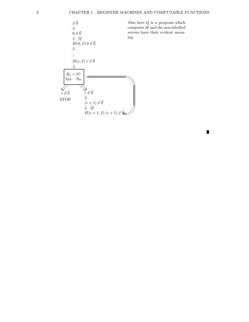
6 CHAPTER 1. REGISTER MACHINES AND COMPUTABLE FUNCTIONS
~x ~0⇓0 ~x ~0⇓ Q
H(0, ~x) 0 ~x ~0⇓...
H(c, ~x) c ~x ~0
R1 = 0?Yes No
⇓
c ~x ~0
STOP
c ~x ~0⇓
(c+ 1) ~x ~0⇓ Q
H(c+ 1, ~x) (c+ 1) ~x ~0
<
Also here Q is a program whichcomputesH and the non-labelledarrows have their evident mean-ing
Chapter 2
Recursive Functions
2.1 Primitive recursive functions and relations
Notation for functions. In mathematical texts, it is common to use expressions containingvariables, such as x+ y, x2, x log y etc., both for a (variable) number and for the function of theoccurring variables: we say “the function x+ y”. However, in Computability Theory, which is toa large extent about ways of defining functions, it is better to distinguish these different meaningsby different notations. The expression x log y may mean, for example:
• a real number
• a function of (x, y), that is a function: R2 → R
• a function of (y, x), i.e. another function: R2 → R
• a function of y (with parameter x, so actually a parametrized family of functions: R → R)
• a function of (x, y, z), that is a function: R3 → R
In order to distinguish these meanings we employ the so-called λ-notation: if ~x is a sequence ofvariables x1 · · ·xk which might occur in the expression G, then λ~x.G denotes the function whichassigns to the k-tuple n1 · · ·nk the value G(n1, . . . , nk) (substitute the ni for xi in G). In thisnotation the 5 meanings above can be distuinguished by notation as follows: x log(y), λxy.x log(y),λyx.x log(y), λy.x log(y) and λxyz.x log(y).
Definition 2.1.1 The class of primitive recursive functions Nk → N (where k is allowed to varyover N) is generated by the following clauses:
i) the number 0 is a 0-ary primitive recursive function;
ii) the zero function Z = λx.0 is primitive recursive;
iii) the successor function S = λx.x+ 1 is primitive recursive;
iv) the projections Πki = λx1 · · ·xk.xi (for 1 ≤ i ≤ k) are primitive recursive;
v) the primitive recursive functions are closed under definition by composition and primitiverecursion.
Recall remark 1.2.4: if H : N2 → N is primitive recursive and n ∈ N, then the function F , definedby
F (0) = nF (y + 1) = H(y, F (y))
is also primitive recursive. The constant n is a primitive recursive 0-ary function, being thecomposition of 0 and n times the function S.
7
8 CHAPTER 2. RECURSIVE FUNCTIONS
Exercise 5 Prove that the primitive recursive functions are total. Prove also that the primitiverecursive functions are computable.
When we speak of a k-ary relation, we mean a subset of Nk. We shall stick to the followingconvention for the characteristic function χA : Nk → N of the k-ary relation A:
χA(~x) =
{0 if ~x ∈ A1 else
A relation is said to be primitive recursive if its characteristic function is.
Examples of primitive recursive functions. The following derivations show for a couple ofsimple functions that they are primitive recursive:
a) λxy.x+ y. For, 0 + y = y = Π11(y), and
(x+1)+ y = S(x+ y) = S(Π32(x, x+ y, y)), hence λxy.x+ y is defined by primitive recursion
from Π11 and a function defined by composition form S and Π3
2;
b) λxy.xy. For, 0y = 0 = Z(y), and(x+1)y = xy+y = (λxy.x+y)(Π3
2(x, xy, y),Π33(x, xy, y)), hence λxy.xy is defined by primi-
tive recursion from Z and a function defined by composition from λxy.x+y and projections;
c) λx.pd(x) (the predecessor function: pd(x) = x− 1 if x > 0, and pd(0) = 0). For, pd(0) = 0,andpd(x+ 1) = x = Π2
1(x, pd(x))
Exercise 6 Prove that the following functions are primitive recursive:
i) λxy.xy
ii) λxy.x−y. This is cut-off subtraction: x−y = x− y if x ≥ y, and x−y = 0 if x < y.
iii) λxy.min(x, y)
iv) sg (the sign function), where
sg(x) =
{1 if x > 00 else
v) sg, where
sg(x) =
{0 if x > 01 else
vi) λxy.|x− y|
vii) λx.n for fixed n
viii) λx.x!
ix) λxy.rm(x, y) where rm(x, y) = 0 if y = 0, and the remainder of x on division by y otherwise.
Exercise 7 Prove that if A is a primitive recursive relation, so is the complement of A.
Exercise 8 Prove that the following relations are primitive recursive:
i) {(x, y) | x = y}
ii) {(x, y) | x ≤ y}
iii) {(x, y) | x|y}
2.1. PRIMITIVE RECURSIVE FUNCTIONS AND RELATIONS 9
iv) {x | x is a prime number}
Exercise 9 Show that the function C is primitive recursive, where C is given by
C(x, y, z) =
{x if z = 0y else
Therefore, we can define primitive recursive functions by ‘cases’, using primitive recursive relations.
Proposition 2.1.2
i) If the function F : Nk+1 → N is primitive recursive, then so are the functions:
λ~xz.∑
y<z F (~x, y)
λ~xz.∏
y<z F (~x, y)
λ~xz.(µy < z.F (~x, y) = 0)
The last of these is said to be defined from F by bounded minimalization, and produces theleast y < z for which F (~x, y) = 0; if such an y < z does not exist, it outputs z);
ii) If A and B are primitive recursive k-ary relations, then so are A ∩B, A ∪B and A−B;
iii) If A is a primitive recursive k + 1-ary relation, then the relations{(~x, z) | ∃y < z(~x, y) ∈ A} and {(~x, z) | ∀y < z(~x, y) ∈ A} are also primitive recursive.
Proof.
a)∑
y<0 F (~x, y) = 0 and∑
y<z+1 F (~x, y) =∑
y<z F (~x, y) + F (~x, z);∏
y<0 F (~x, y) = 1 and∏
y<z+1 F (~x, y) = (∏
y<z F (~x, y))F (~x, z);(µy < 0.F (~x, y) = 0) = 0 and (µy < z + 1.F (~x, y) = 0) = (µy < z.F (~x, y) = 0) +sg(
∏
y<z+1 F (~x, y))
b) χA∩B = λx.sg(χA(x) + χB(x))χA∪B = λx.χA(x)χB(x)
Exercise 10 Finish the proof of Proposition 2.1.2.
Exercise 11 If F : N2 → N is primitive recursive, then so is λn.∑
k<n F (n, k).
Proposition 2.1.3 If G1, G2 and H are primitive recursive functions Nn → N, then so is thefunction F , defined by
F (~x) =
{G1(~x) if H(~x) = 0G2(~x) else
Proof. For, F (~x) = C(G1(~x), G2(~x), H(~x)), where C is the function from exercise 9.
Exercise 12 Let p0, p1, . . . be the sequence of prime numbers: 2, 3, 5, . . . Show that the functionλn.pn is primitive recursive.
10 CHAPTER 2. RECURSIVE FUNCTIONS
2.1.1 Coding of pairs and tuples
One of the basic techniques in Computability Theory is the coding of programs and computationsas numbers.
We shall code sequences of numbers as one number, in such a way that important operationson sequences, such as: taking the length of a sequence, the i-th element of the sequence, forminga sequence out of two sequences by putting one after the other (concatenating two sequences), areprimitive recursive in their codes. This is carried out below.
Any bijection N × N → N is called a pairing function: if f : N × N→N is bijective we saythat f(x, y) codes the pair (x, y). An example of such an f is the primitive recursive functionλxy.2x(2y + 1) − 1.
Exercise 13 Let f(x, y) = 2x(2y+ 1)− 1. Prove that the functions k1 : N → N and k2 : N → N
which satisfy f(k1(x), k2(x)) = x for all x, are primitive recursive.
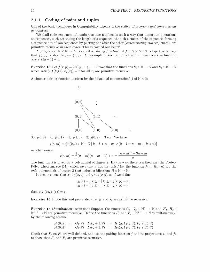
A simpler pairing function is given by the “diagonal enumeration” j of N × N:
...
(0, 2)
""EEEE
EEEE
E...
(0, 1)
##GGGGGGGG(1, 1)
##GGGGGGGG· · ·
(0, 0)
OO
(1, 0)
YY3333333333333333
(2, 0) · · ·
So, j(0, 0) = 0, j(0, 1) = 1, j(1, 0) = 2, j(0, 2) = 3 etc. We have:
j(n,m) = #{(k, l) ∈ N × N | k + l < n+m ∨ (k + l = n+m ∧ k < n)}
in other words
j(n,m) =1
2(n+m)(n+m+ 1) + n =
(n+m)2 + 3n+m
2
The function j is given by a polynomial of degree 2. By the way, there is a theorem (the Fueter-Polya Theorem, see [37]) which says that j and its ‘twist’ i.e. the function λnm.j(m,n) are theonly polynomials of degree 2 that induce a bijection: N × N → N.
It is convenient that x ≤ j(x, y) and y ≤ j(x, y), so if we define:
j1(z) = µx ≤ z.[∃y ≤ z.j(x, y) = z]j2(z) = µy ≤ z.[∃x ≤ z.j(x, y) = z]
then j(j1(z), j2(z)) = z.
Exercise 14 Prove this and prove also that j1 and j2 are primitive recursive.
Exercise 15 (Simultaneous recursion) Suppose the functions G1, G2 : Nk → N and H1, H2 :Nk+3 → N are primitive recursive. Define the functions F1 and F2 : Nk+1 → N ‘simultaneously’by the following scheme:
F1(0, ~x) = G1(~x) F1(y + 1, ~x) = H1(y, F1(y, ~x), F2(y, ~x), ~x)F2(0, ~x) = G2(~x) F2(y + 1, ~x) = H2(y, F1(y, ~x), F2(y, ~x), ~x)
Check that F1 en F2 are well-defined, and use the pairing function j and its projections j1 and j2to show that F1 and F2 are primitive recursive.
2.1. PRIMITIVE RECURSIVE FUNCTIONS AND RELATIONS 11
We are also interested in good bijections: Nn → N for n > 2. In general, such bijections can begiven by polynomials of degree n, but we shall use polynomials of higher degree:
Definition 2.1.4 The bijections jm : Nm → N for m ≥ 1 are defined by:
j1 is the identity functionjm+1(x1, . . . , xm, xm+1) = j(jm(x1, . . . , xm), xm+1)
Then we also have projection functions jmi : N → N for 1 ≤ i ≤ m, satisfying
jm(jm1 (z), . . . , jmm(z)) = z
for all z ∈ N, and given by:
j11(z) = z
jm+1i (z) =
{jmi (j1(z)) if 1 ≤ i ≤ m
j2(z) if i = m+ 1
Exercise 16 Prove:
i) jmi (jm(x1, . . . , xm)) = xi for 1 ≤ i ≤ m; and
ii) the functions jm and jmi are primitive recursive.
Exercise 16 states that for every m and i, the function jmi is primitive recursive. However, thefunctions jmi are connected in such a way, that one is led to suppose that there is also one bigprimitive recursive function which takes m and i as variables. This is articulated more preciselyin the following proposition.
Proposition 2.1.5 The function F , defined by
F (x, y, z) =
{0 if y = 0 or y > x
jxy (z) else
is primitive recursive.
Proof. We first note that the function G(w, z) = (j1)w(z) (the function j1 iterated w times) is
primitive recursive. Indeed: G(0, z) = z and G(w + 1, z) = j1(G(w, z)). Now we have:
F (x, y, z) =
0 if y = 0 or y > xG(x − 1, z) if y = 1
j2(G(x− y, z)) if y > 1
Hence F is defined from the primitive recursive function G by means of repeated distinction bycases.
Exercise 17 Fill in the details of this proof. That is, show that the given definition of F iscorrect, and that from this definition it follows that F is a primitive recursive function
The functions jm and their projections jmi give primitive recursive bijections: Nm → N. Usingproposition 2.1.5 we can now define a bijection:
⋃
m≥0 Nm → N with good properties. An elementof Nm for m ≥ 1 is an ordered m-tuple or sequence (x1, . . . , xm) of elements of N; the uniqueelement of N0 is the empty sequence (−). The result of the function
⋃
m≥0 Nm → N to be defined,on input (x1, . . . , xm) or (−) will be written as 〈x1, . . . , xm〉 or 〈 〉 and will be called the code ofthe sequence.
Definition 2.1.6
〈 〉 = 0〈x0, . . . , xm−1〉 = j(m− 1, jm(x0, . . . , xm−1)) + 1 if m > 0

12 CHAPTER 2. RECURSIVE FUNCTIONS
Exercise 18 Prove that for every y ∈ N the following holds: either y = 0 or there is a uniquem > 0 and a unique sequence (x0, . . . , xm−1) such that y = 〈x0, . . . , xm−1〉.
Remark. In coding arbitrary sequences we have started the convention of letting the indices runfrom 0; this is more convenient and also consistent with the convention that the natural numbersstart at 0.
We now need a few primitive recursive functions for the effective manipulation of sequences.
Definition 2.1.7 The function lh(x) gives us the length of the sequence with code x, and is givenas follows:
lh(x) =
{0 if x = 0
j1(x− 1) + 1 if x > 0
The functions (x)i give us the i-th element of the sequence with code x (count from 0) if 0 ≤ i <lh(x), and 0 otherwise, and is given by
(x)i =
{
jlh(x)i+1 (j2(x− 1)) if 0 ≤ i < lh(x)
0 else
Exercise 19 Prove that the functions λx.lh(x) and λxi.(x)i are primitive recursive;Show that (〈x0, . . . , xm−1〉)i = xi and that (〈 〉)i = 0;Show that for all x: either x = 0 or x = 〈(x)0, . . . , (x)lh(x)−1〉.
The concatenation function gives for each x and y the code of the sequence which we obtain byputting the sequences coded by x and y after each other, and is written x ⋆ y. That means:
〈 〉 ⋆ y = yx ⋆ 〈 〉 = x
〈(x)0, . . . , (x)lh(x)−1〉 ⋆ 〈(y)0, . . . (y)lh(y)−1〉 = 〈(x)0, . . . (x)lh(x)−1, (y)0,. . . , (y)lh(y)−1〉
Exercise 20 Show that λxy.x ⋆ y primitive recursive. (Hint: you can first define a primitiverecursive function λxy.x ◦ y, satisfying
x ◦ y = x ⋆ 〈y〉
Then, define by primitive recursion a function F (x, y, w) by putting
F (x, y, 0) = xF (x, y, w + 1) = F (x, y, w) ◦ (y)w
Finally, put x ⋆ y = F (x, y, lh(y)). )
Course-of-values recursion The scheme of primitive recursion:
F (y + 1, ~x) = H(y, F (y, ~x), ~x)
allows us to define the value of F (y+ 1, ~x) directly in terms of F (y, ~x). Course-of-values recursionis a scheme which defines F (y + 1, ~x) in terms of all previous values F (0, ~x), . . . , F (y, ~x).
Definition 2.1.8 Let G : Nk → N and H : Nk+2 → N be functions. The function F : Nk+1 → N,defined by the clauses
F (0, ~x) = G(~x)
F (y + 1, ~x) = H(y, F (y, ~x), ~x)
where F (y, ~x) = 〈F (0, ~x), . . . , F (y, ~x)〉
is said to be defined from G and H by course-of-values recursion.
2.1. PRIMITIVE RECURSIVE FUNCTIONS AND RELATIONS 13
Proposition 2.1.9 Suppose G : Nk → N and H : Nk+2 → N are primitive recursive functionsand F : Nk+1 → N is defined from G and H by course-of-values recursion. Then F is primitiverecursive.
Proof. SinceF (0, ~x) = 〈G(~x)〉
F (y + 1, ~x) = F (y, ~x) ∗ 〈H(y, F (y, ~x), ~x)〉
the function F is primitive recursive. Now
F (y, ~x) = (F (y, ~x))y
so F is primitive recursive too.
We might also consider the following generalization of the course-of-values recursion scheme: in-stead of allowing only the values F (w, ~x) for w ≤ y to be used in the definition of F (y + 1, ~x), we
could allow all values F (w, ~x′) (for w ≤ y). This should be well-defined, for inductively we havealready defined all functions Fw = λ~x.F (w, ~x) when we are defining Fy+1. That this is indeed
possible (and does not lead us outside the class of primitive recursive functions) if ~x′ is a primitiverecursive function of ~x, is shown in the following exercise.
Exercise 21 Let K : N → N, G : Nk+1 → N and H : Nk+3 → N be functions. Define F by:
F (0, ~y, x) = G(~y, x)F (z + 1, ~y, x) = H(z, F (z, ~y,K(x)), ~y, x)
Suppose that G, H and K are primitive recursive.
a) Prove directly, suitably adapting the proof of proposition 2.1.9: if ∀x(K(x) ≤ x), then F isprimitive recursive.
b) Define a new function F ′ by:
F ′(0,m, ~y, x) = G(~y,Km(x))
F ′(n+ 1,m, ~y, x) = H(n, F ′(n,m, ~y, x), ~y,Km−(n+1)(x))
Recall that Km−(n+1) means: the function K applied m−(n+ 1) times.
Prove: if n ≤ m then ∀k[F ′(n,m+ k, ~y, x) = F ′(n,m, ~y,Kk(x))]
c) Prove by induction: F (z, ~y, x) = F ′(z, z, ~y, x) and conclude that F is primitive recursive,also without the assumption that K(x) ≤ x.
Double recursion. However, the matter is totally different if, in the definition of F (y+1, ~x), weallow values of Fy at arguments in which already known values of Fy+1 may appear. In this casewe speak of double recursion. We treat a simple case, with a limited number of variables.
Definition 2.1.10 Let G : N → N, H : N2 → N, K : N4 → N, J : N → N, en L : N3 → N befunctions; the function F is said to be defined from these by double recursion if
F (0, z) = G(z)F (y + 1, 0) = H(y, F (y, J(y)))
F (y + 1, z + 1) = K(y, z, F (y + 1, z), F (y, L(y, z, F (y+ 1, z))))
Proposition 2.1.11 If G, H, K, J and L are primitive recursive and F is defined from these bydouble recursion as in definition 2.1.10 then all functions Fy = λz.F (y, z) are primitive recursive,but F itself need not be primitive recursive.
14 CHAPTER 2. RECURSIVE FUNCTIONS
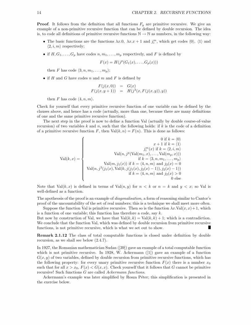
Proof. It follows from the definition that all functions Fy are primitive recursive. We give anexample of a non-primitive recursive function that can be defined by double recursion. The ideais, to code all definitions of primitive recursive functions N → N as numbers, in the following way:
• The basic functions are the functions λx.0, λx.x + 1 and jmi , which get codes 〈0〉, 〈1〉 and〈2, i,m〉 respectively;
• if H,G1, . . . , Gp have codes n,m1, . . . ,mp respectively, and F is defined by
F (x) = H(jp(G1(x), . . . , Gp(x)))
then F has code 〈3, n,m1, . . . ,mp〉;
• if H and G have codes n and m and F is defined by
F (j(x, 0)) = G(x)F (j(x, y + 1)) = H(j3(x, F (j(x, y)), y))
then F has code 〈4, n,m〉.
Check for yourself that every primitive recursive function of one variable can be defined by theclauses above, and hence has a code (actually, more than one, because there are many definitionsof one and the same primitive recursive function).
The next step in the proof is now to define a function Val (actually by double course-of-valuerecursion) of two variables k and n, such that the following holds: if k is the code of a definitionof a primitive recursive function F , then Val(k, n) = F (n). This is done as follows:
Val(k, x) =
0 if k = 〈0〉x+ 1 if k = 〈1〉
jmi (x) if k = 〈2, i,m〉Val(n, jp(Val(m1, x), . . . ,Val(mp, x)))
if k = 〈3, n,m1, . . . ,mp〉Val(m, j1(x)) if k = 〈4, n,m〉 and j2(x) = 0
Val(n, j3(j1(x),Val(k, j(j1(x), j2(x) − 1)), j2(x) − 1))if k = 〈4, n,m〉 and j2(x) > 0
0 else
Note that Val(k, x) is defined in terms of Val(n, y) for n < k or n = k and y < x; so Val iswell-defined as a function.
The apotheosis of the proof is an example of diagonalisation, a form of reasoning similar to Cantor’sproof of the uncountability of the set of real numbers; this is a technique we shall meet more often.
Suppose the function Val is primitive recursive. Then so is the function λx.Val(x, x)+1, whichis a function of one variable; this function has therefore a code, say k.But now by construction of Val, we have that Val(k, k) = Val(k, k) + 1; which is a contradiction.We conclude that the function Val, which was defined by double recursion from primitive recursivefunctions, is not primitive recursive, which is what we set out to show.
Remark 2.1.12 The class of total computable functions is closed under definition by doublerecursion, as we shall see below (2.4.7).
In 1927, the Romanian mathematician Sudan ([39]) gave an example of a total computable functionwhich is not primitive recursive. In 1928, W. Ackermann ([1]) gave an example of a functionG(x, y) of two variables, defined by double recursion from primitive recursive functions, which hasthe following property: for every unary primitive recursive function F (x) there is a number x0
such that for all x > x0, F (x) < G(x, x). Check yourself that it follows that G cannot be primitiverecursive! Such functions G are called Ackermann functions.
Ackermann’s example was later simplified by Rosza Peter; this simplification is presented inthe exercise below.

2.1. PRIMITIVE RECURSIVE FUNCTIONS AND RELATIONS 15
Exercise 22 (Ackermann-Peter) Define by double recursion:
A(0, x) = x+ 1A(n+ 1, 0) = A(n, 1)
A(n+ 1, x+ 1) = A(n,A(n+ 1, x))
Again we write An for λx.A(n, x). For a primitive recursive function F : Nk → N, we say that F isbounded by An, written F ∈ B(An), if for all x1, . . . , xk we have F (x1, . . . , xk) < An(x1 + · · ·+xk).Prove by inductions on n and x:
i) n+ x < An(x)
ii) An(x) < An(x+ 1)
iii) An(x) < An+1(x)
iv) An(An+1(x)) ≤ An+2(x)
v) nx+ 2 ≤ An(x) for n ≥ 1
vi) λx.x+ 1, λx.0 and λ~x.xi ∈ B(A1)
vii) if F = λ~x.H(G1(~x), . . . , Gp(~x)) and H,G1, . . . , Gp ∈ B(An) for some n > p, then F ∈B(An+2)
viii) for every n ≥ 1 we have: if F (0, ~x) = G(~x) and F (y + 1, ~x) = H(y, F (y, ~x), ~x) and G,H ∈B(An), then F ∈ B(An+3)
Concluide that for every primitive recursive function F there is a number n such that F ∈ B(An);hence, that A is an Ackermann function.
Exercise 23 Define a sequence of functions G0, G1, . . . : N → N by
G0(y) = y + 1Gx+1(y) = (Gx)
y+1(y)
and then define G by putting G(x, y) = Gx(y). Give a definition of G by double rcursion andcomposition (use a definition scheme for double recursion which allows an extra variable) andprove that G is an Ackermann function.
A few simple exercises to conclude this section:
Exercise 24 Show that the following “recursion scheme” does not define a function:
F (0, 0) = 0F (x+ 1, y) = F (y, x+ 1)F (x, y + 1) = F (x+ 1, y)
Exercise 25 Show that the following “recursion scheme” is not satisfied by any function:
F (0, 0) = 0F (x+ 1, y) = F (x, y + 1) + 1F (x, y + 1) = F (x+ 1, y) + 1
16 CHAPTER 2. RECURSIVE FUNCTIONS
2.1.2 A Logical Characterization of the Primitive Recursive Functions
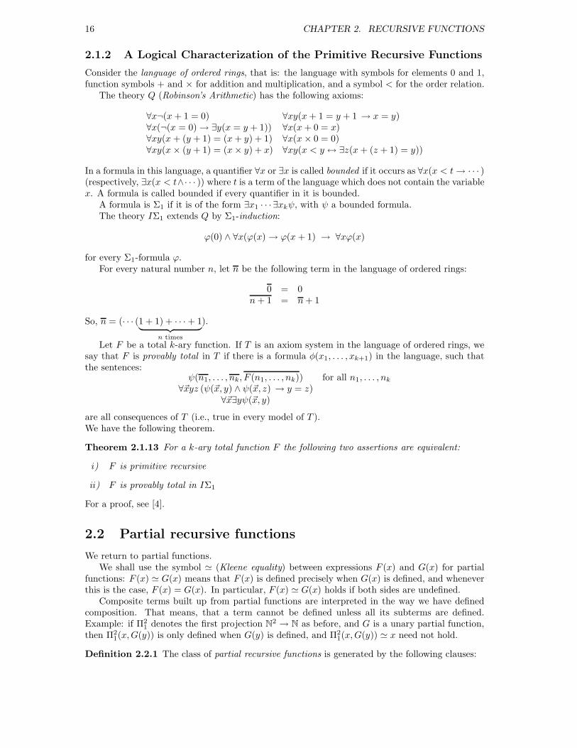
Consider the language of ordered rings, that is: the language with symbols for elements 0 and 1,function symbols + and × for addition and multiplication, and a symbol < for the order relation.
The theory Q (Robinson’s Arithmetic) has the following axioms:
∀x¬(x + 1 = 0) ∀xy(x+ 1 = y + 1 → x = y)∀x(¬(x = 0) → ∃y(x = y + 1)) ∀x(x + 0 = x)∀xy(x + (y + 1) = (x+ y) + 1) ∀x(x × 0 = 0)∀xy(x × (y + 1) = (x× y) + x) ∀xy(x < y ↔ ∃z(x+ (z + 1) = y))
In a formula in this language, a quantifier ∀x or ∃x is called bounded if it occurs as ∀x(x < t→ · · · )(respectively, ∃x(x < t∧· · · )) where t is a term of the language which does not contain the variablex. A formula is called bounded if every quantifier in it is bounded.
A formula is Σ1 if it is of the form ∃x1 · · · ∃xkψ, with ψ a bounded formula.The theory IΣ1 extends Q by Σ1-induction:
ϕ(0) ∧ ∀x(ϕ(x) → ϕ(x + 1) → ∀xϕ(x)
for every Σ1-formula ϕ.For every natural number n, let n be the following term in the language of ordered rings:
0 = 0n+ 1 = n+ 1
So, n = (· · · (1 + 1) + · · · + 1︸ ︷︷ ︸
n times
).
Let F be a total k-ary function. If T is an axiom system in the language of ordered rings, wesay that F is provably total in T if there is a formula φ(x1, . . . , xk+1) in the language, such thatthe sentences:
ψ(n1, . . . , nk, F (n1, . . . , nk)) for all n1, . . . , nk∀~xyz (ψ(~x, y) ∧ ψ(~x, z) → y = z)
∀~x∃yψ(~x, y)
are all consequences of T (i.e., true in every model of T ).We have the following theorem.
Theorem 2.1.13 For a k-ary total function F the following two assertions are equivalent:
i) F is primitive recursive
ii) F is provably total in IΣ1
For a proof, see [4].
2.2 Partial recursive functions
We return to partial functions.We shall use the symbol ≃ (Kleene equality) between expressions F (x) and G(x) for partial
functions: F (x) ≃ G(x) means that F (x) is defined precisely when G(x) is defined, and wheneverthis is the case, F (x) = G(x). In particular, F (x) ≃ G(x) holds if both sides are undefined.
Composite terms built up from partial functions are interpreted in the way we have definedcomposition. That means, that a term cannot be defined unless all its subterms are defined.Example: if Π2
1 denotes the first projection N2 → N as before, and G is a unary partial function,then Π2
1(x,G(y)) is only defined when G(y) is defined, and Π21(x,G(y)) ≃ x need not hold.
Definition 2.2.1 The class of partial recursive functions is generated by the following clauses:
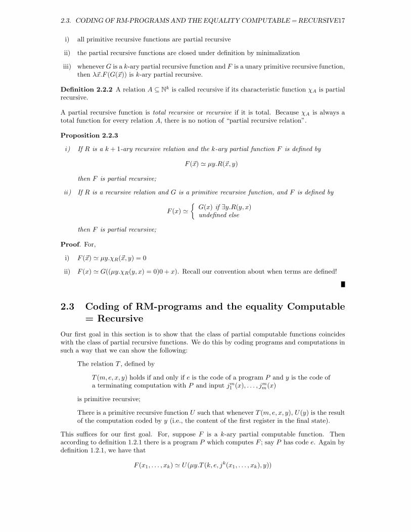
2.3. CODING OF RM-PROGRAMS AND THE EQUALITY COMPUTABLE = RECURSIVE17
i) all primitive recursive functions are partial recursive
ii) the partial recursive functions are closed under definition by minimalization
iii) wheneverG is a k-ary partial recursive function and F is a unary primitive recursive function,then λ~x.F (G(~x)) is k-ary partial recursive.
Definition 2.2.2 A relation A ⊆ Nk is called recursive if its characteristic function χA is partialrecursive.
A partial recursive function is total recursive or recursive if it is total. Because χA is always atotal function for every relation A, there is no notion of “partial recursive relation”.
Proposition 2.2.3
i) If R is a k + 1-ary recursive relation and the k-ary partial function F is defined by
F (~x) ≃ µy.R(~x, y)
then F is partial recursive;
ii) If R is a recursive relation and G is a primitive recursive function, and F is defined by
F (x) ≃
{G(x) if ∃y.R(y, x)undefined else
then F is partial recursive;
Proof. For,
i) F (~x) ≃ µy.χR(~x, y) = 0
ii) F (x) ≃ G((µy.χR(y, x) = 0)0 + x). Recall our convention about when terms are defined!
2.3 Coding of RM-programs and the equality Computable
= Recursive
Our first goal in this section is to show that the class of partial computable functions coincideswith the class of partial recursive functions. We do this by coding programs and computations insuch a way that we can show the following:
The relation T , defined by
T (m, e, x, y) holds if and only if e is the code of a program P and y is the code ofa terminating computation with P and input jm1 (x), . . . , jmm(x)
is primitive recursive;
There is a primitive recursive function U such that whenever T (m, e, x, y), U(y) is the resultof the computation coded by y (i.e., the content of the first register in the final state).
This suffices for our first goal. For, suppose F is a k-ary partial computable function. Thenaccording to definition 1.2.1 there is a program P which computes F ; say P has code e. Again bydefinition 1.2.1, we have that
F (x1, . . . , xk) ≃ U(µy.T (k, e, jk(x1, . . . , xk), y))
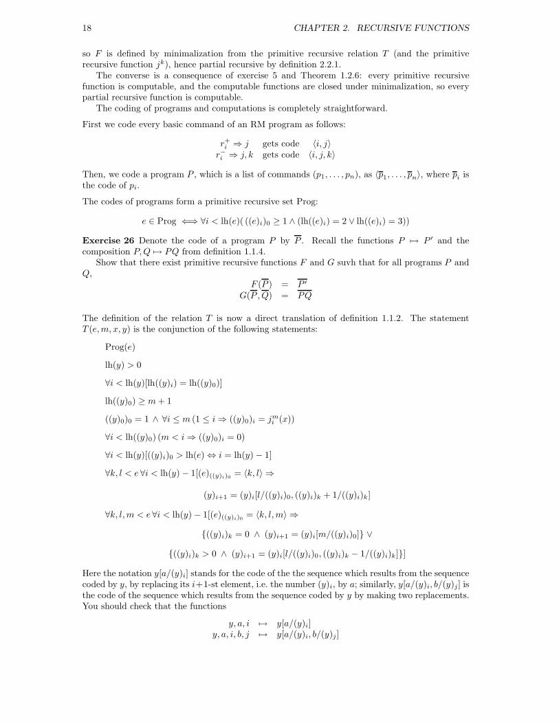
18 CHAPTER 2. RECURSIVE FUNCTIONS
so F is defined by minimalization from the primitive recursive relation T (and the primitiverecursive function jk), hence partial recursive by definition 2.2.1.
The converse is a consequence of exercise 5 and Theorem 1.2.6: every primitive recursivefunction is computable, and the computable functions are closed under minimalization, so everypartial recursive function is computable.
The coding of programs and computations is completely straightforward.
First we code every basic command of an RM program as follows:
r+i ⇒ j gets code 〈i, j〉r−i ⇒ j, k gets code 〈i, j, k〉
Then, we code a program P , which is a list of commands (p1, . . . , pn), as 〈p1, . . . , pn〉, where pi isthe code of pi.
The codes of programs form a primitive recursive set Prog:
e ∈ Prog ⇐⇒ ∀i < lh(e)( ((e)i)0 ≥ 1 ∧ (lh((e)i) = 2 ∨ lh((e)i) = 3))
Exercise 26 Denote the code of a program P by P . Recall the functions P 7→ P ′ and thecomposition P,Q 7→ PQ from definition 1.1.4.
Show that there exist primitive recursive functions F and G suvh that for all programs P andQ,
F (P ) = P ′
G(P ,Q) = PQ
The definition of the relation T is now a direct translation of definition 1.1.2. The statementT (e,m, x, y) is the conjunction of the following statements:
Prog(e)
lh(y) > 0
∀i < lh(y)[lh((y)i) = lh((y)0)]
lh((y)0) ≥ m+ 1
((y)0)0 = 1 ∧ ∀i ≤ m (1 ≤ i⇒ ((y)0)i = jmi (x))
∀i < lh((y)0) (m < i⇒ ((y)0)i = 0)
∀i < lh(y)[((y)i)0 > lh(e) ⇔ i = lh(y) − 1]
∀k, l < e ∀i < lh(y) − 1[(e)((y)i)0 = 〈k, l〉 ⇒
(y)i+1 = (y)i[l/((y)i)0, ((y)i)k + 1/((y)i)k]
∀k, l,m < e ∀i < lh(y) − 1[(e)((y)i)0 = 〈k, l,m〉 ⇒
{((y)i)k = 0 ∧ (y)i+1 = (y)i[m/((y)i)0]} ∨
{((y)i)k > 0 ∧ (y)i+1 = (y)i[l/((y)i)0, ((y)i)k − 1/((y)i)k]}]
Here the notation y[a/(y)i] stands for the code of the the sequence which results from the sequencecoded by y, by replacing its i+1-st element, i.e. the number (y)i, by a; similarly, y[a/(y)i, b/(y)j] isthe code of the sequence which results from the sequence coded by y by making two replacements.You should check that the functions
y, a, i 7→ y[a/(y)i]y, a, i, b, j 7→ y[a/(y)i, b/(y)j]

2.3. CODING OF RM-PROGRAMS AND THE EQUALITY COMPUTABLE = RECURSIVE19
are primitive recursive.Convince yourself, by going over these statements, that T (e,m, x, y) has the intended meaning,
and that it is primitive recursive.Because the result of a computation is the number stored in the first register when the machine
stops, the functionU(y) = ((y)lh(y)−1)1
gives the result; and U is clearly primitive recursive.The letters T and U are standard in Computability Theory. The relation T is also called the
Kleene T -predicate and U is often called the output function.We summarize our observations in the following theorem.
Theorem 2.3.1 (Enumeration Theorem)
i) A partial function is computable if and only if it is partial recursive.
ii) Define the partial recursive function Φ by
Φ(m, e, x) ≃ U(µy.T (m, e, x, y))
Then for every k-ary partial recursive function F there is a number e such that for allk-tuples x1, . . . , xk:
F (x1, . . . , xk) ≃ Φ(k, e, jk(x1, . . . , xk))
In other words, we have a partial recursive enumeration of the partial recursive functions.
Corollary 2.3.2 The partial recursive functions are closed under composition and primitive re-cursion.
Since the function Φ from Theorem 2.3.1 is partial recursive, there is a program which computesit; such a program is called a universal program.
By contrast, there is no analogous theorem for total recursive functions:
Proposition 2.3.3 There is no total recursive function Ψ(m, e, x) witrh the property that forevery k-ary total recursive function F there is a number e such that
F = λx1 · · ·xm.Ψ(m, e, jm(x1, . . . , xm))
Proof. For suppose such a function Ψ exists; we argue by diagonalization as in the proof ofproposition 2.1.11. The function
G(x1 · · ·xm) = Ψ(m, jm(x1, . . . , xm), jm(x1, . . . , xm)) + 1
is total recursive, and therefore there should be an e such that for all x1, . . . , xm: G(x1 · · ·xm) =Ψ(m, e, jm(x1, . . . , xm)). However, for such e we would have
Ψ(m, e, e) = Ψ(m, e, jm(jm1 (e), . . . , jmm(e))) = G(jm1 (e), . . . , jmm(e)) = Ψ(m, e, e) + 1
which is a clear contradiction.
Exercise 27 Show that for every m-ary partial recursive function F there exist infinitely manynumbers e such that
F = λx1 · · ·xm.Φ(m, e, jm(x1, . . . , xm))
Exercise 28 Let R1, . . . , Rn ⊆ Nk be recursive relations such that Ri ∩ Rj = ∅ for i 6= j; letG1, . . . , Gn be k-ary partial recursive functions. Then the partial function F , defined by
F (~x) ≃
G1(~x) if R1(~x)...
...Gn(~x) if Rn(~x)
undefined else
is also partial recursive; prove this.
20 CHAPTER 2. RECURSIVE FUNCTIONS
2.4 Smn-Theorem and Recursion Theorem
If F = λx1 · · ·xm.Φ(m, e, jm(x1, . . . , xm)), then e is called an index for F , and we write φe (or
sometimes φ(m)e if we want to make the arity of F explicit) for F .
However, subscripts are a bore, especially in compound terms, and therefore we shall writee·(x1, . . . , xm) for φe(x1, . . . , xm)1.
The following theorem has an odd name: “Smn-theorem”. A better name would be “para-metrization theorem”. If we have an (m + n)-ary partial recursive function φe and m numbersa1, . . . , am, then the n-ary partial function (x1, . . . , xn) 7→ φe(a1, . . . , am, x1, . . . , xn) is also par-tial recursive. The theorem says that an index for this last partial function can be obtainedprimitive-recursively in e and a1, . . . , am. We sketch a proof.
Theorem 2.4.1 (Smn-theorem; Kleene) For every m ≥ 1 and n ≥ 1 there is an m + 1-aryprimitive recursive function Smn such that for all e, x1, . . . , xm, y1, . . . , yn:
Smn (e, x1, . . . , xm)·(y1, . . . , yn) ≃ e·(x1, . . . , xm, y1, . . . , yn)
Proof. If e is not the code of an RM-program we put Smn (e, x1, . . . , xm) = e. If e codes a programP , then for every x1, . . . , xm, the number Smn (e, x1, . . . , xm) should code a program that performsthe following computation:
b1 · · · bnremove junk ⇓
b1 · · · bn~0input register contents ~x ⇓ (R+
1 )x1 · · · (R+m)xm
x1 · · ·xm b1 · · · bn⇓ Pe·(x1, . . . , xm, b1, . . . bn)~c
(Here, (R+i )n is the program that adds 1 to the i-th register n times) It is left to you to convince
yourself that Smn is primitive recursive.
The result of the following exercise will be used in the sequel!
Exercise 29 Show, by modifying the proof of Theorem 2.4.1 a bit, that the function Smn can beassumed to be injective.
We have already noted (corollary 2.3.2) that the partial recursive functions are closed undercomposition. The following corollary of Theorem 2.4.1 states that one can find an index fora composition G◦F of partial recursive functions, primitive-recursively in indices for G and F .We restrict to the case of composition of two unary functions; the general case is left to you toformulate and prove.
Corollary 2.4.2 There is a primitive recursive function H such that for all e, f, x the followingholds:
H(e, f)·x ≃ e·(f ·x)
Proof. The function λefx.e·(f ·x) is partial recursive. Indeed,
e·(f ·x) ≃ U(j2(µz.[T (1, f, x, j1(z)) ∧ T (1, e, U(j1(z)), j2(z))]))
Therefore, there exists a number g such that e·(f ·x) ≃ g·(e, f, x) for all e, f, x; put H(e, f) =S2
1(g, e, f)
Exercise 30 Formulate and prove a generalization of corollary 2.4.2 for arbitrary compositions(as in definition 1.2.2).
1Kleene invented the terrible notation {e}(x1, . . . , xm)
2.4. SMN -THEOREM AND RECURSION THEOREM 21
The following theorem is a surprising consequence of the Smn-theorem. It allows us to define apartial recursive function F in terms of an index for F !
Theorem 2.4.3 (Recursion Theorem, Kleene 1938) For every k ≥ 1 and k + 1-ary partialrecursive function F there exists an index e such that for all x1, . . . , xk the following holds:
e·(x1, . . . xk) ≃ F (x1, . . . , xk, e)
Moreover, there is a primitive recursive function which produces such an e for every index of F .
Proof. Suppose f is an index for F , so f ·(x1, . . . , xk+1) ≃ F (x1, . . . , xk+1) for all x1, . . . , xk+1.Now, choose an index g satisfying for all h, y, x1, . . . , xk:
g·(h, y, x1, . . . , xk) ≃ h·(x1, . . . , xk, S1k(y, y))
(Such g exists because the function on the right hand side is clearly partial recursive)Now let
e = S1k(S
1k+1(g, f), S1
k+1(g, f))
Clearly, e depends primitive-recursively on f . Moreover,
e·(x1, . . . , xk) ≃S1k(S
1k+1(g, f), S1
k+1(g, f))·(x1, . . . , xk) ≃ by the Smn-theoremS1k+1(g, f)·(S1
k+1(g, f), x1, . . . , xk) ≃g·(f, S1
k+1(g, f), x1, . . . , xk) ≃ by choice of gf ·(x1, . . . , xk, S
1k(S
1k+1(g, f), S1
k+1(g, f))) ≃ by definition of ef ·(x1, . . . , xk, e) ≃ by assumption on fF (x1, . . . , xk, e)
Theorem 2.4.3 is often called (e.g. in [26]) the Second Recursion Theorem. The First RecursionTheorem is Theorem 2.4.5 below.
Corollary 2.4.4 Let G be k-ary partial recursive, and H k + 2-ary partial recursive. Then anindex for the function F which is defined from G and H by primitive recursion, can be foundprimitive-recursively in indices for G and H.
Proof. The function
L(g, h, y, ~x, f) ≃
{g·(~x) if y = 0h·(y − 1, f ·(y − 1, ~x), ~x) if y > 0
is clearly partial recursive; let l be an index for L. By Theorem 2.4.3 we can find an indexf such that for all y, ~x we have: f ·(y, ~x) ≃ S2
k+2(l, g, h)·(y, ~x, f). And moreover, f is foundprimitive-recursively in S2
k+2(l, g, h) hence primitive rcursively in g, h.Applying the Smn-theorem, we find that f ·(y, ~x) ≃ L(g, h, y, ~x, f) and thus, if g and h are indicesfor G and H respectively, that f is an index for the function defined from G and H by primitiverecursion.
The recursive relations are closed under bounded quantifiers: if R ⊆ Nk+1 is recursive, then soare
{(~x, y) | ∀w < y.R(~x,w)}
and{(~x, y) | ∃w < y.R(~x,w)}
because their characteristic functions are defined by primitive recursion from those of R (seeproposition 2.1.2iii) ). And again, an index for the characteristic function of a relation definedby bounded quantification from R can be obtained primitive-recursively from an index for thecharacteristic function of R.

22 CHAPTER 2. RECURSIVE FUNCTIONS
Exercise 31
i) Show that for every recursive relation R, there is an e such that for all ~x:
e·(~x) ≃
{0 if R(~x, e)1 else
ii) Show that for every recursive relation R and every partial recursive function F , there is ane such that for all ~x:
e·(~x) ≃
{F (~x) if ∃y.R(~x, y, e)
undefined else
The following theorem is often called (e.g. in [26]) the First Recursion Theorem, or FixpointTheorem.
Corollary 2.4.5 (Fixpoint Theorem) For every total recursive function F and every n thereis a number e such that e and F (e) are indices for the same n-ary partial recursive function:
φ(n)e = φ
(n)F (e)
Proof. Let G be the partial recursive function defined by
G(~x, e) ≃ F (e)·(~x)
Apply Theorem 2.4.3 to find an index e satisfying
e·(~x) ≃ G(~x, e)
Remark 2.4.6 Of course, Corollary 2.4.5 is not a “Fixpoint Theorem” in the usual sense of theword: there is no operation of which it is asserted that this operation has a fixed point. Observethat the function F is not an operation on partial recursive functions, but only on indices.
Exercise 32 Prove the primitive recursive version of corollary 2.4.5. That is: there is a primitiverecursive function T satisfying for all f and ~x:
T (f)·(~x) ≃ (f ·T (f))·(~x)
Exercise 33 Prove the recursion theorem with parameters : there is a primitive recursive functionF satisfying for all f, ~y, ~x:
F (f, ~y)·(~x) ≃ f ·(F (f, ~y), ~y, ~x)
and also: there is a primitive recursive F ′ such that for all f, ~y, ~x:
F ′(f, ~y)·(~x) ≃ (f ·(F ′(f, ~y), ~y))·(~x)
Remark 2.4.7 We conclude this chapter with the promised proof that the class of total com-putable functions is closed under definition by double recursion. Assume therefore that G,H, J,Kand L are total recursive, and that the function F is defined by:
F (0, z) = G(z)F (y + 1, 0) = H(y, F (y, J(y)))
F (y + 1, z + 1) = K(y, z, F (y + 1, z), F (y, L(y, z, F (y+ 1, z))))
Then F is total recursive, for by theorem 2.4.3 we can find an index f satisfying
f ·(y, z) ≃
G(z) if y = 0H(y − 1, f ·(y − 1, J(y − 1))) if y > 0
and z = 0K(y − 1, z − 1, f ·(y, z − 1), f ·(y − 1, L(y − 1, z − 1, f ·(y, z − 1)))) if y > 0
and z > 0
2.4. SMN -THEOREM AND RECURSION THEOREM 23
Exercise 34 Prove by double induction (on y and z) that the function φf is total and equal toF .
One more exercise.
Exercise 35 Prove Smullyan’s Simultaneous Recursion Theorem: given two binary partial recur-sive functions F and G, for every k there exist indices a and b satisfying for all x1, . . . , xk:
a·(x1, . . . , xk) ≃ F (a, b)·(x1, . . . , xk)
andb·(x1, . . . , xk) ≃ G(a, b)·(x1, . . . , xk)
24 CHAPTER 2. RECURSIVE FUNCTIONS
Chapter 3
Undecidability and Recursively
Enumerable Sets
3.1 Solvable Problems
Every subset of Nk constitutes a “problem”: the problem of determining whether a given k-tupleof natural numbers belongs to the set. For example the set
{(f, x) | ∃zT (1, f, x, z)}
is the problem of deciding whether or not f ·x is defined.We call a problem (i.e., set) solvable if the set is recursive. Another word is decidable.The above mentioned problem: is f ·x defined?, is classical and is called the Halting Problem
(Turing): is the computation on the RM with program coded by f and input x finite?
Proposition 3.1.1 The Halting Problem is not solvable.
Proof. Suppose for a contradiction that we have a total recursive function F satisfying for allf, x:
F (f, x) ≃
{0 if f ·x is defined1 otherwise
Let G be a partial recursive function such that dom(G) = N−{0} (for example, G(x) ≃ µz.xz > 1).Then by the Recursion Theorem (2.4.3) there is an index f such that for all x the following holds:
f ·x ≃ G(F (f, x))
But then, surely f ·x is defined if and only if F (f, x) 6= 0; which is the case if and only if f ·x isundefined. We have the desired contradiction.
There is a simpler proof. The Standard Problem is: is x·x defined?Clearly, if we can solve the Halting problem, then we can solve the Standard Problem, as you
can check for yourself. Now suppose the Standard Problem is solvable. Then we have a totalrecursive function F such that for all x the following holds:
F (x) ≃
{0 if x·x is defined1 otherwise
LetG be as in the proof of 3.1.1, and let f be an index for the partial recursive function λx.G(F (x)).We then have: f ·f is defined if and only if F (f) = 0, which is the case if and only if G(F (f)),
which is equal to f ·f , is undefined; contradiction. So it was not really necessary to appeal to theRecursion Theorem in the proof of 3.1.1.
25
26 CHAPTER 3. UNDECIDABILITY AND RECURSIVELY ENUMERABLE SETS
The relation between the Standard Problem and the Halting Problem is an example of reducibilityof one problem to another: if R ⊆ Nm and S ⊆ Nk are problems then R is said to be reducibleto S if there exist k m-ary total recursive functions F1, . . . , Fk such that for every m-tuple ~x wehave:
~x ∈ R ⇔ (F1(~x), . . . , Fk(~x)) ∈ S
Exercise 36 Show: if R is reducible to S and S is solvable, then so is R.
Later on, we shall deal with reducibility in more detail. A variation of the notion of solvability issolvability with respect to. The problem is then, to determine whether ~x ∈ R for ~x ∈ A. We say:is R solvable with respect to A?
Definition 3.1.2 LetR and A be subsets of Nk. We say thatR is solvable with respect to A if thereis a k-ary partial recursive function F such that A ⊆ dom(F ) and for all ~x ∈ A, F (~x) = χR(~x).
Example 3.1.3 Denote the range of a function F by rge(F ). The problem: is 0 ∈ rge(φe)?, isnot solvable with respect to {e |φe is total}.
Proof. We must show that there is no partial recursive function F which satisfies the following:whenever φe is total, F (e) is defined and we have:
F (e) =
{0 if there exists a z such that e·z = 01 otherwise
Let g be an index such that for all x, y:
g·(x, y) ≃
{0 if T (1, x, x, y)1 otherwise
Then S11(g, x) is the index of a total recursive function, for S1
1(g, x)·y ≃ g·(x, y). We have:
0 ∈ rge(φS11(g,x)) ⇔ ∃y.T (1, x, x, y) ⇔ x·x is defined
Therefore, if such an F existed, the function G = λx.F (S11 (g, x)) would be a solution of the
Standard Problem; which contradicts 3.1.1.
Exercise 37 Prove that the problem: is φe total?, is not solvable.[Hint: first define a total recursive function F such that for all e the following holds: e·e is definedif and only if φF (e) is total. Then conclude the statement from this]
Exercise 38 Prove that the following problems are undecidable:
i) dom(φe) = ∅?
ii) rge(φe) infinite?
iii) φe = φf?
Exercise 39 Determine which of the following problems are solvable with respect to indices oftotal functions:
i) ∃x.e·x 6= 0
ii) ∃x.e·x ≤ e·(x+ 1)
iii) ∃x.e·x ≥ e·(x+ 1)
iv) e·x = y (as ternary relation)
3.1. SOLVABLE PROBLEMS 27
v) φe has infinite range
Exercise 40 Show that there is no binary total recursive function F such that for all e, x thefollowing holds:
e·x is defined =⇒ ∃y(T (1, e, x, y) ∧ lh(y) ≤ F (e, x))
[Hint: show that there is a primitive recursive function S(e, x, n) such that S(e, x, n) gives the firstn stages of a computation of the RM with a program with code e and input x, provided Prog(e);then, conclude from existence of an F as described, that the Halting Problem is decidable]
Exercise 41 Show that there is no total recursive function F which satisfies the following, for alle: if φe is the characteristic function of a finite set, then F (e) is an upper bound for this set.
[Hint: consider the set {lh(µy.T (1, e, x, y))}. Show that an index for the characteristic function ofthis set can be obtained primitive-recursively in e and x]
Definition 3.1.4 A subset X of N is called extensional for indices of partial recursive functions(or extensional for short) if for all e, f ∈ N the following holds:
if φe = φf and e ∈ X then also f ∈ X
Another terminology one encounters in the literature, is index set.
Note, that the properties in exercise 39 are all extensional.
Rice’s Theorem says that nontrivial extensional properties of indices for partial recursive functionscan never be decidable:
Theorem 3.1.5 (Rice) If X ⊆ N is recursive and extensional, then X = ∅ or X = N.
Proof. Note that if X is recursive and extensional, then so is its complement; therefore, ifX 6= ∅, X 6= N then we may assume that all indices for the empty partial function are notmembers of X . Let f be such an index, and pick e ∈ X .By the Smn-Theorem there is a primitive recursive function F such that for all x, y:
F (x)·y ≃
{e·y if ∃zT (1, x, x, z)
undefined else
We have:If x·x is defined then φF (x) = φe, so F (x) ∈ X ; and if x·x is undefined, then φF (x) = φf , soF (x) 6∈ X . Therefore the Standard Set {x |x·x is defined} is reducible to X via F . Hence Xcannot ne decidable.
For lovers of the Recursion Theorem an alternative proof of Theorem 3.1.5: Let X be recursiveand extensional, e ∈ X, f 6∈ X with f an index for the empty function. By the Recursion Theoremthere is an index g such that for all x the following holds:
g·x ≃
{f ·x if g ∈ Xe·x otherwise
Since X is extensional we then have:
g ∈ X ⇒ φg = φf ⇒ g 6∈ Xg 6∈ X ⇒ φg = φe ⇒ g ∈ X
which is a contradiction.
28 CHAPTER 3. UNDECIDABILITY AND RECURSIVELY ENUMERABLE SETS
3.2 Recursively Enumerable Sets
From our point of view the recursive sets are the simplest problems: they are solvable. One stepup, we find the recursively enumerable (also called: computably enumerable) sets.
Definition 3.2.1 A subset X of N is called recursively enumerable (abbreviated: r.e.) if there isa partial recursive function ψ such that R = dom(ψ).
Proposition 3.2.2 The following four statements are equivalent for a subset R of N:
i) R is recursively enumerable
ii) There is a recursive relation S ⊆ N2 such that R = {x | ∃y((x, y) ∈ S)}
iii) There is a partial recursive function F such that R = rge(F )
iv) R = ∅ or there is a primitive recursive function F such that R = rge(F )
Moreover, the implications i)⇒ii)⇒iii)⇒i) are primitive-recursively uniform in indices. Thismeans, for example, for i)⇒ii), that there is a primitive recursive function G such that, wheneverf is an index for a partial recursive function which testifies that R is recursively enumerable, thenG(f) is an index for the characteristic function of a relation S which testifies ii).
Proof. i)⇒ii). Suppose R = dom(ψ); let f be an index for ψ. Then R = {x | ∃yT (1, f, x, y)};because T is primitive recursive, there is an index g such that for all h, x, y:
g·(h, x, y) ≃
{0 if T (1, f, x, y)1 otherwise
It follows that dom(φf ) = {x | ∃y(S12(g, f)·(x, y) = 0)}, and φS1
2(g,f) is always an index for a
characteristic function.
ii)⇒iii). We can choose an index g, such that whenever f is an index for a characteristic functionF and R = {x | ∃y(f ·(x, y) = 0)}, then for all x the following holds:
g·(f, x) ≃
{x if ∃y(f ·(x, y) = 0)
undefined otherwise
It is left to you to check that R = rge(φS11(g,f)).
iii)⇒i). Suppose R = rge(φf ). Then R = dom(φS11(g,f)), where g is an index such that for all f, x:
g·(f, x) ≃
{0 if ∃y[T (1, f, j1(y), j2(y)) and U(j2(y)) = x]
undefined otherwise
iv)⇒iii) is clear.
iii)⇒iv). If R = rge(F ) then either R = ∅ or there is some a ∈ R. In the first case we are done;in the other case, let f be an index for F , and let g be an index such that
g·(f, y) ≃
{a if ¬T (1, f, j1(y), j2(y))
U(j2(y)) if T (1, f, j1(y), j2(y))
Then R = rge(φS11(g,f)), and φS1
1(g,f) is clearly primitive recursive.
The equivalence of statement iv) of proposition 3.2.2 to the other statements cannot be madeprimitive-recursively uniform in indices, because of the case distinction whether rge(φf ) = ∅ ornot. This cannot be decided recursively, as we saw (exercise 38i) ).
3.2. RECURSIVELY ENUMERABLE SETS 29
Remark 3.2.3 We extend the definition of r.e. sets to subsets of Nk by saying that a k-ary relationR is r.e. if R is the domain of a k-ary partial recursive function.We have the following notation for r.e. sets:
W ke = dom(φ(k)
e )
If R = W ke then e is said to be an r.e. index for R.
We often write We instead of W(1)e .
Exercise 42 Prove: a k-ary relation R is r.e. if and only if {jk(x1, . . . , xk) | ~x ∈ R} is an r.e.subset of N.
Example 3.2.4
i) The unsolvability of the Standard Problem means that the set
K = {x | x·x is defined}
is not recursive; K is r.e. for K = {x | ∃y.T (1, x, x, y)} hence satisfies ii) of proposition 3.2.2(the symbol K is standard in the literature, for this set).
ii) Every recursive set is r.e.
Exercise 43 Prove: if S is r.e. and R is reducible to S, then R is r.e.
Exercise 44 Prove that {e | φe is total} is not r.e.
Exercise 45 Prove that every r.e. set is of the form {x | ∃y((x, y) ∈ S)} for some primitiverecursive S ⊆ N2.
Proposition 3.2.5 (Post)
i) R ⊆ Nk is recursive if and only if both R and its complement are r.e.;
ii) N −K = {x | x·x is undefined} is not r.e.;
iii) A k-ary partial function is partial recursive if and only if its graph: {(~x, y) | F (~x) = y}, isr.e.;
iv) if a k-ary function is total recursive, then its graph is recursive.
Proof.
i) If R is recursive, then so is its complement, so both are r.e.
Conversely, if R = {~x | ∃yS(~x, y)} and Nk−R = {~x | ∃y.T (~x, y)} for recursive S and T , thendefine a partial recursive k-ary function F by F (~x) ≃ µy.(S(~x, y) ∨ T (~x, y)). The functionF is total and we have: ~x ∈ R if and only if (~x, F (~x)) ∈ S. Hence R is recursive.
ii) This follows from i) because if N −K were r.e. then K would be recursive, which is not thecase.
iii) Let f be an index for F . The graph of F is
{(~x, y) | y = F (~x)} = {(~x, y) | ∃w[T (k, f, jk(~x), w) and U(w) = y]}
and is therefore r.e.; conversely, if
{(~x, y) | y = F (~x)} = {(~x, y) | ∃zS(~x, y, z)}
for some recursive S, then F = φg, where g is an index such that
∀~x[g·(~x) ≃ j1(µz.S(~x, j1(z), j2(z)))]
30 CHAPTER 3. UNDECIDABILITY AND RECURSIVELY ENUMERABLE SETS
iv) The graph of F is r.e. by iii) but since F is total, the complement of the graph of F is
{(~x, y) | ∃z[T (k, f, jk(~x), z) and U(z) 6= y]}
for any index f for F ; and is therefore also r.e. Hence the graph of F is recursive by i).
Exercise 46 Prove that statement i) van proposition 3.2.5 holds primitive-recursively uniform inindices, that is: there is a binary primitive recursive function T such that, whenever Wx is thecomplement of Wy then χWx
= φT (x,y).
Exercise 47
i) Use the Recursion Theorem in order to show that for every total recursive function F thereis a number n such that WF (n) = Wn; deduce from this that there exists an n such thatWn = {n} and that there is an n such that Wn = {m | m > n}.
ii) Prove, using the Recursion Theorem, that there is a total recursive function F with theproperties ∀n(F (n) < F (n+ 1)) and ∀n(WF (n) = {F (n+ 1)}).
Exercise 48 Prove:
i) If a total recursive function F is nondecreasing and has infinite range, then rge(F ) is recur-sive.
ii) Every infinite r.e. set contains an infinite recursive subset.
Do these results hold primitive-recursively uniform in indices?
Propositie 3.2.5ii) shows that the r.e. are not closed under complements. Exercise 44 implies thatthey are neither closed under arbitrary intersections (for {e | ϕe is total} =
⋂
x∈N{e | ∃yT (1, e, x, y)})
or unions (for A =⋃
x∈A{x} for every set A, and every singleton set is of course r.e.). We do havethe following:
Proposition 3.2.6
i) If R and S are r.e. then so are R ∪ S and R ∩ S;
ii) if R ⊆ Nk+1 is r.e. then so is
{(~x, z) ∈ Nk+1 | ∀w < zR(~x,w)}
iii) if R ⊆ N is r.e. then so is⋃
x∈RWx.
These results are primitive-recursively uniform in indices (that is, e.g. for i): Wx ∩Wy = WF (x,y)
and Wx ∪Wy = WG(x,y) for primitive recursive functions F and G.).
Exercise 49 Prove proposition 3.2.6. For ii): use coding of sequences in order to replace aquantifier combination ∀w < z∃y by a combination ∃y∀w < z.
Exercise 50 [Reduction Theorem] Prove that for every couple of r.e. sets X,Y ⊆ N there existr.e. sets X ′ en Y ′ such that the following hold:
i) X ′ ⊆ X and Y ′ ⊆ Y ;
ii) X ′ ∩ Y ′ = ∅;
iii) X ′ ∪ Y ′ = X ∪ Y .
3.2. RECURSIVELY ENUMERABLE SETS 31
Hint: if X = We and Y = Wf , let
X ′ = {x | ∃y(T (1, e, x, y) and ∀z < y¬T (1, f, x, z))}
Definition 3.2.7 Two r.e. sets X,Y are called recursively inseparable if there is no recursive setR with X ⊆ R and R ∩ Y = ∅ (equivalently, if there is no total recursive function F such thatF (x) = 0 for all x ∈ X and F (x) > 0 for all x ∈ Y ).
Proposition 3.2.8 Recursively inseparable r.e. sets exist.
Proof. Define
X = {x | x·x = 0} = {x | ∃y[T (1, x, x, y) and U(y) = 0]}Y = {x | x·x = 1}
We shall show that there is a primitive recursive function F with the following property: alsX ⊆ We, Y ⊆ Wf and We ∩ Wf = ∅, then F (e, f) 6∈ We ∪ Wf (Check that this implies thestatement! Use proposition 3.2.5i)).Let g be an index such that for all e, f, x:
g·(e, f, x) ≃
1 if ∃y[T (1, e, x, y) and ∀w ≤ y¬T (1, f, x, w)]0 if ∃y[T (1, f, x, y) and ∀w < y¬T (1, e, x, w)]
undefined otherwise
Define F (e, f) = S21(g, e, f) and let e and f be such that X ⊆ We, Y ⊆ Wf and We ∩Wf = ∅.
Then we have:if S2
1(g, e, f) ∈ We then
S21(g, e, f)·S2
1(g, e, f) = g·(e, f, S21(g, e, f)) = 1
hence S21(g, e, f) ∈ Y , contradiction;
if S21(g, e, f) ∈ Wf then
S21(g, e, f)·S2
1(g, e, f) = 0
hence S21(g, e, f) ∈ X ; with a similar contradiction.
We conclude that S21(g, e, f) 6∈ We ∪Wf , as desired.
Exercise 51 [Extension Problem] Show that there exist partial recursive functions which cannotbe extended to a total recursive function.
Exercise 52 An r.e. set X is called creative via a partial recursive function F if for every e thefollowing holds:
If We ∩X = ∅ then F (e) is defined and F (e) 6∈ X ∪We
Show that for the sets X en Y from the proof of proposition 3.2.8 there exist partial recursivefunctions F and G such that X and Y are creative via F and G, respectively.
3.2.1 The Kleene Tree
A tree is (for us, here) a set T of finite sequences of natural numbers which is closed under initialsegments: if (s0, . . . , sn) ∈ T and m ≤ n then also (s0, . . . , sm) ∈ T . We also consider the emptysequence (−), which is an initial segment of any sequence.A tree is finitely branching if for every sequence (s0, . . . , sn−1) ∈ T there are only finitely manynumbers a such that (s0, . . . , sn−1, a) ∈ T .A path through a tree T is a total function F such that for all n, (F (0), . . . , F (n)) ∈ T .A tree is called recursive if the set of codes of elements of T (in the sense of coding of sequences)is recursive.In the context of arbitrary (not necessarily recursive) trees we have the following classical fact:

32 CHAPTER 3. UNDECIDABILITY AND RECURSIVELY ENUMERABLE SETS
Proposition 3.2.9 (Konig’s Lemma) Let T be a finitely branching tree. If T is infinite, thenthere is a path through T .
Proof. If s is an element of T , by Ts we denote the set of those elements of T which are eitheran initial segment of s or have s as initial segment. Clearly, Ts is a tree.Assume T is finitely branching and infinite. Then T is nonempty so the empty sequence is in T ;since T is finitely branching there are finitely many numbers a such that (a) ∈ T ; say a0, . . . , ak.Then
T =
k⋃
i=0
T(ai)
which is a finite union of sets; since T is infinite we can find an i such that T(ai) is infinite; letF (0) = ai for the least such i.Inductively, we have defined F (0), . . . , F (n) in such a way that T(F (0),...,F (n)) is infinite. This treeis also finitely branching, so again, there are finitely many a0, . . . , ak such that
T(F (0),...,F (n)) =k⋃
i=0
T(F (0),...,F (n),ai)
and again we can pick F (n+ 1) = ai such that T(F (0),...,F (n),ai) is infinite.
You can check that the function F is well-defined and a path through T .
The situation is different when we consider recursive trees and recursive paths:
Theorem 3.2.10 (Kleene Tree) There is an infinite, finitely branching, recursive tree throughwhich there is no recursive path.
Proof. Let T be the set of those sequences (a0, . . . , an−1) which satisfy:
for all i < n, ai ≤ 1for all i, k < n, if T (1, i, i, k) and U(k) ≤ 1, then ai = U(k)
Convince yourself that T is a tree, and that it is recursive. By the first requirement on elements ofT , T is finitely branching. In order to construct an element of T of length n, simply run throughall i, k < n and check whether T (i, 1, i, k) and U(k) ≤ 1. If so, put ai = U(k). This gives afinite number of constraints on the sequence we wish to construct; if there is no such constraintinvolving the number i, simply put ai = 0. So we get a legitimate element of T of length n; henceT is infinite.Now suppose F is a recursive path through T . Suppose x·x = 0. Let k be such that T (1, x, x, k).Let n > max(x, k). Then since (F (0), . . . , F (n)) ∈ T we must have F (x) = 0. Similarly, whenx·x = 1 we must have F (x) = 1. Also, F takes values in {0, 1}. We conclude that F is a recursiveseparation of the sets X and Y in the proof of proposition 3.2.8, contradicting that proposition.
3.3. EXTENSIONAL R.E. SETS AND EFFECTIVE OPERATIONS 33
3.3 Extensional r.e. sets and effective operations
In this section you’ll find three important theorems on extensional r.e. sets of indices of partialrecursive functions and indices of r.e. sets, and “effective operations” on these things. Let usclarify what we mean by this.
Definition 3.3.1 A subset A of N is called extensional for indices of r.e. sets if whenever e ∈ Aand We = Wf , then f ∈ A.
Write PR for the set of all partial recursive functions, R for the set of total recursive functions,and RE for the set of r.e. subsets of N. A function H : PR → PR, R → R or RE → RE is calledan effective operation if there is a partial recursive function F such that:
if H : PR → PR then F is total, and for all e, H(φe) = φF (e)
if H : R → R then {e |φe is total} ⊆ dom(F ) and for all e, H(φe) = φF (e)
if H : RE → RE then F is total and for all e: H(We) = WF (e)
In a similar way, one can define effective operations RE → PR, R → N etc.In this section we shall show that there exist very natural topologies on the sets PR, R and RE ,such that the following statements are true:
every r.e. extensional set for indices of partial recursive functions is open in PR
every r.e. extensional set for indices of r.e. sets is open in RE
every effective operation is continuous
The topology we take on R is straightforward. Give N the discrete topology, and then the set offunctions NN, which is the same as the infinite profuct
∏
n∈NN, the product topology. A basis for
this topology is given by the sets
Us = {f : N → N | f(0) = s0, . . . , f(n− 1) = sn−1}
for every finite sequence s = (s0, . . . , sn−1) of numbers.The set R, as subset of NN, now gets the subspace topology, which has as basis the sets Us∩R.
For RE , we do something more subtle. When we have numbers n and e, the problem “is n anelement of We?” is, as we know, in general undecidable. We do have a program that, on inputs nand e, outputs 0 if n ∈We (the program searches for the first y such that T (1, e, n, y) and outputs0 if such y is found); but for n 6∈ We the program will never tell us anything. We therefore choosea topology on RE which mirrors this fact.
Identify P(N), the powerset of N, with the set of functions N → {0, 1} via characteristicfunctions. This is also a product:
∏
n∈N{0, 1}, but this time we do not give {0, 1} the discrete
topology; instead, we give it the Sierpinski topology which has 3 open sets: ∅, {0} and {0, 1}.Then, endow {0, 1}N with the product topology. This results in a topology on P(N) for which thefollowing sets form a basis:
UA = {X ⊆ N |A ⊆ X}
where A ⊂ N is finite.Finally, RE , as subset of P(N), gets the subspace topology.
Exercise 53 Let V ⊆ RE . Prove that V is open in RE if and only if the following two statementshold:
i) V is upwards closed: if X ∈ V , Y ∈ RE and X ⊆ Y , then Y ∈ V
ii) whenever X ∈ V , there is a finite subset A ⊆ X such that A ∈ V .
34 CHAPTER 3. UNDECIDABILITY AND RECURSIVELY ENUMERABLE SETS
For PR we note that this set can be seen as a subset of RE via the map which sends a partialrecursive function to its graph (which as an r.e. set). Therefore, we give PR the subspace topologyof RE . A basis for the topology on PR is given by sets
Us = {ϕ partial recursive | ∀i < lh(s) (ϕ(j1(si)) = j2(si))}
where s is such that for all i, j < lh(s), if j1(si) = j1(sj) then si = sj.
Again, a set of V of partial recursive functions is open if and only if V is upwards closed andsatisfies the condition that whenever a function F is in V , there is a finite subfunction G of Fwhich is in V .
Proposition 3.3.2
a) A function F : R → R is continuous if and only if for every total recursive function f andevery finite sequence s such that F (f) ∈ Us, there is a finite sequence t such that f ∈ Ut andF maps Ut into Us.
b) A function F : RE → RE or PR → PR is continuous if and only if the following twoconfitions hold:
i) F is monotone: whenever S ⊆ T , F (S) ⊆ F (T )
ii) F is compact: whenever A ⊆ F (S) is finite, there is a finite subset B of S such thatA ⊆ F (B)
Exercise 54 Prove proposition 3.3.2.
3.3.1 Theorems of Myhill-Shepherdson, Rice-Shapiro and Kreisel-Lacombe-
Shoenfield
In the following theorem, parts 1 and 2 are known as the Myhill-Shepherdson Theorem, and 3 and4 form the Rice-Shapiro Theorem
Theorem 3.3.3 (Myhill-Shepherdson; Rice-Shapiro)
1) Let R be r.e. and extensional for indices of partial recursive functions. Then the set
{φe | e ∈ R}
is open in PR
2) Let F : PR → PR be an effective operation. Then F is continuous
3) Let R be r.e. and extensional for indices of r.e. sets. Then the set
{We | e ∈ R}
is open in RE
4) Let F : RE → RE be an effective operation. Then F is continuous
Proof. 1). We have to show the following two things:
a) If e ∈ R and φe ⊆ φf then f ∈ R
b) If e ∈ R then there is a number e′ such that φe′ is finite, φe′ ⊆ φe, and e′ ∈ R
3.3. EXTENSIONAL R.E. SETS AND EFFECTIVE OPERATIONS 35
Let h be an index for the r.e. set R.For a), use the Recursion Theorem to pick an index g such that for all e, f, x the following
holds:
g·(e, f, x) ≃U(j2(µz.[j1z = 0 and T (1, e, x, j2z)] or
[T (1, h, S21(g, e, f), j1z) and T (1, f, x, j2z)]))
Now suppose e ∈ R. First we see that S21(g, e, f) ∈ R. For if not, no z will ever satisfy the second
part of the disjunction in the definition of g·(e, f, x). That means that for all x,
S21(g, e, f)·x ≃ U(j2(µz.[j1z = 0 and T (1, e, x, j2z)])) ≃ e·x
so φS21(g,e,f) = φe. But e ∈ R, and R is extensional. This is a contradiction. Therefore,
S21(g, e, f) ∈ R.
Now suppose furthermore that φe ⊆ φf . We observe that g·(e, f, x) ≃ f ·x always (check!), soφS2
1(g,e,f) = φf . Since S2
1(g, e, f) ∈ R and R is extensional, we have f ∈ R, as desired.For b), use the Recursion Theorem to pick an index g such that for all e, x:
g·(e, x) ≃
{e·x if for no k ≤ x, T (1, h, S1
1(g, e), k)undefined otherwise
Assume e ∈ R. Again, we see that S11(g, e) must be an element of R, for otherwise we have
S11(g, e)·x ≃ g·(e, x) ≃ e·x
so φS11(g,e) = φe, and we get a contradiction with the extensionality of R.
Now we know that S11(g, e) ∈ R, let k be the least such that T (1, h, S1
1(g, e), k). Then from thedefinition we see that g·(e, x) is undefined for x ≥ k, so S1
1(g, e) is the index of a finite function.Moreover, the inclusion φS1
1(g,e) ⊆ φe is immediate from the definition.
2). We show directly that the preimage F−1(Us) is open in PR, where Us is a typical basis elementfor the topology on PR:
Us = {ϕ partial recursive | ∀i < lh(s) (ϕ(j1(si)) = j2(si))}
where s is such that for all i, j < lh(s), if j1(si) = j1(sj) then si = sj.Let f be an index such that F (φe) = φf ·e for all e. Then we have that φe ∈ F−1(Us) if and
only if
∀i < lh(s) ((f ·e)·j1(si) is defined and equal to j2(si))
We see that {e |φe ∈ F−1(Us)} is r.e. It is also clearly extensional, because F is an effectiveoperation. So the openness of F−1(Us) follows from part 1.
3). Suppose R is r.e. and extensional for indices of r.e. sets. Then R is also extensional for indicesof partial recursive functions, because φe = φf implies We = Wf . Hence, by 1), the set
P = {φe | e ∈ R}
is open in PR. Therefore, if e ∈ R there is some e′ ∈ R such that φe′ ⊆ φe and φe′ is finite. Thenalso We′ is finite, and We′ ⊆We.
Furthermore, if e ∈ R and We ⊆Wf , we have the partial recursive functions
ϕe(x) ≃
{0 if x ∈ We
undefined otherwiseand ϕf (x) ≃
{0 if x ∈Wf
undefined otherwise
Any index for ϕe belongs to R since dom(ϕe) = We; so by openness of the set P , any index forϕf belongs to R. Hence f ∈ R.
36 CHAPTER 3. UNDECIDABILITY AND RECURSIVELY ENUMERABLE SETS
4). We have continuous maps I : RE → PR and J : PR → RE defined by: I(We) is the functionϕe from the proof of 3), and J(ϕ) = dom(ϕ). An index for ϕe can be found primitive-recursivelyin e: if g is an index such that
g·(e, x) ≃
{0 if x ∈We
undefined otherwise
then S11(g, e) is an index for ϕe. Also, J(φe) = We. It follows from this, that when F : RE → RE
is an effective operation, then the composition IFJ : PR → PR is also an effective operation, andhence continuous by 2). Because the functions I and J are continuous, the composition J(IFJ)Iis a continuous map RE → RE . But this map is just F , because the composition JI is the identitymap on RE .
Note that we have actually proven a primitive-recursively uniformity result: there is a primitiverecursive function S(h, e) such that whenever R = Wh is extensional and e ∈ R, then S(h, e) is anindex for a finite set (or function) which is in R and contained in We (φe).
Exercise 55 Conclude from Theorem 3.3.3 that there cannot exist a total recursive function Fwhich is such that for all e: φe is constant on its domain if and only if F (e) ∈ K.
Exercise 56 Conclude from Theorem 3.3.3 that there cannot exist a total recursive function Fwhich is such that for all e: We is a singleton set precisely when F (e) ∈ K.
Exercise 57 Conclude from Theorem 3.3.3 that neither {x |Wx is finite} nor {x |Wx is infinite}are r.e.
The situation for R is a bit more subtle. Recall that the basic opens are of the form Us zijn, met
Us = {f ∈ R | ∀i < lh(s) f(i) = (s)i}
Call a set X extensioneel for indices of total functions, if for every pair e, e′ of indices of totalfunctions we have:
If φe = φe′ then (e ∈ X ⇔ e′ ∈ X)
The result on r.e. extensional sets being open, fails in this context. First of all we have:
Exercise 58 Show: if X is an r.e. set of indices of total recursive functions and X is extensionalfor indices of total recursive functions, then X = ∅.
But we can modify the question: suppose we do not require that X consist only of indices fortotal functions. Do we have that if X is r.e. and extensional for indices of total functions, the set
{φe |φe is total and e ∈ X}
is open in R? The answer is no, as the following proposition shows.
Proposition 3.3.4 (Friedberg, 1958) There exists an r.e. set X which is extensional for in-dices of total functions, such that {φe |φe is total and e ∈ X} is not open in R.
Proof. Define sets Y and Z by
Y = {e | ∀x ≤ e.e·x = 0}Z = {e | ∃z[e·z > 0 and ∀y < z.e·y = 0 and
∃e′ < z∀u ≤ z.e′·u = e·u]}
Let X = Y ∪Z. Since both Y and Z are r.e., so is X . Also, note that Z is extensional for indicesof total functions. In order to see that X is extensional for indices of total functions, supposeφe = φe′ , φe and φe′ are total, and e ∈ X .
If φe′ = λx.0 then e′ ∈ Y , hence e′ ∈ X . If not, let y′ the minimal x for which φe′ (x) > 0. Wedistinguish two cases:
3.3. EXTENSIONAL R.E. SETS AND EFFECTIVE OPERATIONS 37
a) e ∈ Y . Then since φe = φe′ , we have ∀x ≤ e.e′·x = 0, so e < y′.
If y′ ≤ e′ then e′ ∈ Z (switch the roles of e and e′ in the definition of Z, and take y′ for z).
If e′ < y′, then e′ ∈ Y . We conclude that if e ∈ Y then always e′ ∈ X .
b) e ∈ Z. Then e′ ∈ Z by extensionality of Z, hence also e′ ∈ X .
However, the set T = {φe ∈ R | e ∈ X} is not open in R: because λx.0 ∈ T we would have, if Twere open, an s such that ∀i < lh(s).(s)i = 0 ∧ Us ⊆ T ; choose such an s and let n = lh(s). Nowlet g be an index such that for all x:
g·x ≃
{0 if x < nk otherwise
where k 6= 0 is determined in such a way that no partial recursive function with index < n hasthe same values as φg on the set {0, . . . , n}. We have: φg ∈ Us, but n ≤ g (check!), and g 6∈ X .
Exercise 59 Show that if X is r.e. and extensional for indices of partial recursive functions, thenthe set
{φe |φe is total and e ∈ X}
is open in R.
We do have the continuity result, for which the most important building block is the theorem ofKreisel-Lacombe-Shoenfield (independently also proved by the Russian Ceitin).
Theorem 3.3.5 (Kreisel, Lacombe, Shoenfield (1957)) There is a partial recursive functionK with the following property: for every effective operation F : R → N (effective in the sense thatF (φe) = f ·e for a certain index f) and every f satisfying
{e | φe is total} ⊆ dom(φf ) and ∀e(if φe is total then f ·e = F (φe))
and for every e such that φe is total, K(f, e) is defined, and the following holds:
1. φe ∈ UK(f,e)
2. ∀e′(if φe′ is total and φe′ ∈ UK(f,e) then F (φe) = F (φe′ ))
Proof. Let s◦ = λx.(s)x (Recall that by convention, (s)x = 0 for x ≥ lh(s), so s◦ is a totalfunction); let G be primitive recursive such that s◦ = φG(s). We define a partial recursive functionof 4 variables as follows:
η(f, y, z, x) ≃
undefined if f ·y is undefined (1)y·x if ¬∃w ≤ x(T (1, f, z, w) and U(w) = f ·y) (2)
s◦(x) if w ≤ x is minimal such that T (1, f, z, w) and U(w) = f ·y,and 〈s, t〉 is minimal such that lh(s) > w andand ∀i < w∃v < t(T (1, y, i, v) and U(v) = (s)i) and (3)and ∃v < t(T (1, f, G(s), v) and U(v) 6= f ·y)
undefined if in (3) such a 〈s, t〉 does not exist
We apply the Recursion Theorem to find an index z such that for all f, y, x:
z·(f, y, x) ≃ η(f, y, S21(z, f, y), x)
Now suppose that F is an effective operation, and f an index such that F (ϕe) = f ·e for everyindex e of a total recursive function, and assume φy is total. Then f ·y is defined. Moreover wehave:
i) There exists a w such that T (1, f, S21(z, f, y), w) and U(w) = f ·y. For if not, then S2
1(z, f, y)·xequals y·x for all x (this follows from the definition of η, for S2
1(z, f, y)·x ≃ η(f, y, S21(z, f, y), x)),
i.e. φS21(z,f,y) = φy , but then we should have f ·S2
1(z, f, y) = f ·y, by the assumption on f .
38 CHAPTER 3. UNDECIDABILITY AND RECURSIVELY ENUMERABLE SETS
ii) Let w be minimal such that T (1, f, S21(z, f, y), w). Then there cannot exist an s such that
w ≤ lh(s) and ∀i < w.y·i = (s)i and f ·G(s) 6= f ·y
For suppose such s existed. Then there would be 〈s, t〉 as in (3) of the definition of η, whichwould imply that φS2
1(z,f,y) = φG(s) = s◦ so f ·S2
1(z, f, y) = f ·G(s) 6= f ·y, which contradictsi).
iii) With w as in ii) we have: if φy′ is total ∀i < w.y′·i = y·i, then f ·y = f ·y′; for if w′ satisfiesT (1, f, S2
1(z, f, y′), w′) and w′′ is the maximum of w and w′we have:
f ·y′ = f ·G(〈y′·0, . . . , y′·(w′ − 1)〉)
because of ii) with y′ substituted for y; this also equals f ·G(〈y′·0, . . . , y′·(w′′ − 1)〉) = f ·y,for 〈y′·0, . . . , y′·(w′′ − 1)〉 is an extension of the sequence 〈y·0, . . . , y·(w − 1)〉.
So if we put:K(f, y) ≃ 〈y·0, . . . , y·(v − 1)〉
where v = µw.T (1, f, S21(z, f, y), w), then K has the stated properties of the theorem. Check
yourself that K is partial recursive.
Corollary 3.3.6 Let F : R → R be an effective operation. Then F is continuous.
Proof. This is immediate from Theorem 3.3.5: for each n, the function which sends f to F (f)(n)is an effective operation R → N, hence continuous. Therefore, by the defining property of theproduct topology, F is continuous as map R → NN; and since it lands in R and R has the subspacetopology, F is continuous as map R → R.
However, we can make a stronger statement. Call a map F : R → R effectively continuous if thereis a partial recursive function ϕ such that for every pair (e, n) with φe total, ϕ(e, n) is defined andthe following holds:
F [U〈e·0,...,e·ϕ(e,n)〉 ⊆ U〈F (φe)(0),...,F (φe)(n)〉
Corollary 3.3.7 Let F : R → R be an effective operation. Then F is effectively continuous.
Proof. We must show that for every f ∈ R and every s such that F (f) ∈ Us, there is a v suchthat f ∈ Uv and F [Uv] ⊆ Us.Because F is an effective operation, there is a partial recursive function ψ such that for all i andall indices of total recursive functions e:
ψ(e, i) = F (ϕe)(i)
Let G be primitive recursive, such that G(i) is an index for λe.ψ(e, i); we have:
φe = φe′ ⇒ G(i)·e = G(i)·e′
for all i and all indices for total recursive functions e, e′; therefore we can apply Theorem 3.3.5 toG(i). Let f ∈ R, f = φy . Let
w = max{lh(K(G(i), y)) | 0 ≤ i < lh(u)}
Then the following holds:If g ∈ U〈y·0,...,y·(w−1)〉 then F (g) ∈ Us
(check!)
Remark 3.3.8 The number w = wy,s = max{lh(K(G(i), y)) | 0 ≤ i < lh(s)} is sometimes calleda modulus of continuity of F at φy. However we should keep in mind that it crucially depends onthe index y; that is, in general there is no partial recursive function N which satisfies: N(y, u) isa modulus van continuity, and if φy = φy′ then N(y, s) = N(y′, s).
Exercise 60 Show that there does not exist a subset A ⊆ N and an effective operation F : R → N
which satisfies for all indices for total recursive functions e:
0 ∈ rge(φe) if and only if F (e) ∈ A

3.4. STRICT R.E. SETS IN MATHEMATICS AND LOGIC 39
3.4 Strict r.e. sets in Mathematics and Logic
In this section we discuss a number of problems in Mathematics and Logic, the unsolvability ofwhich has been demonstrated using techniques from Recursion Theory. In every example there isa suitable coding of the problem in terms of natural numbers.
3.4.1 Hilbert’s Tenth Problem
As mentioned in the Introduction, in 1900 David Hilbert presented a list with problems for the20th century. The tenth problem was about Diophantine equations , that is: equations of theform P (X1, . . . , Xn) = 0, waar P ∈ Z[X1, . . . , Xn] is a polynomial with integer coefficients. Theproblem reads:
10. Given a Diophantine equation in an arbitrary number of variables and with integercoefficients; design a procedure by which it can be deternmined in a finite number ofsteps whether the equation has a solution in the integers.
Now every polynomial in n variables can of course be coded as a sequence of n + 1-tuples (forcoefficients and powers), for example: give 4X4
1X2 + 5X22X3 +X1X3 code
〈〈4, 4, 1, 0〉, 〈5, 0, 2, 1〉, 〈1, 1, 0, 1〉〉
in such a way that if pPq denotes the code of the polynomial P , the function
λx1 · · ·xn.P (x1, . . . , xn)
is primitive recursive in pPq and x1, . . . , xn. The set
{u | u = pPq and ∃~x.P (~x) = 0}
is then obviously r.e. A solution to Hilbert’s Tenth Problem presupposes that the set of all u suchthat u codes a polynomial P for which the equation P (~x) = 0 has integer solutions, is recursive.
In 1970, after much preparatory work by Davis, Julia Robinson, and Putnam, the Russian YuriMatyasevich proved that for every e and n there is a polynomial P in at least n + 1 variabblesand with integer coefficients, such that
Wne = {(x1, . . . , xn) | ∃an+1 · · ·an+kP (x1, . . . , xn, an+1, . . . , an+k) = 0}
It now follows that
the setWne is nonempty, precisely when the corresponding polynomial P (X1, . . . , Xn+k)
has integer zeroes
and therefore, a solution of Hilbert’s Tenth Problem in full generality would yield a decisionprocedure for the problem: is Wn
e = ∅? But we have seen, that this problem is unsolvable.A proof of Matyasevich’s Theorem can be found in the very accessible book [24]; there is also
a proof in [37].Interestingly, this theorem initiated a development that is still going on today. Number-
theorists got interested in the question: what if one replaces (in the statement of Hilbert’s problem)Z by Q? Or, if one replaces Z by the ring of integers of a number field? These problems are morecomplicated than the original one, and involve study of elliptic curves and algebraic geometry. Fora survey of results and open questions, see [28].
3.4.2 Word Problems: Groups
Word problems arise with every type of mathematical structure which is defined by generatorsand relations. As an example, I sketch the word problem for groups.
40 CHAPTER 3. UNDECIDABILITY AND RECURSIVELY ENUMERABLE SETS
Let A = {a1, . . . , an} be a finite set. Let f : A → B be a bijection, where B is disjoint fromA. We shall write A−1 for B and a−1 for f(a).
A word on A is a sequence of elements of A ∪ A−1 in which never two elements ai, a−1i (or
a−1i , ai appear consecutively. We also consider the empty sequence as a word. Let [A] be the
collection of words on AWe can concatenate two words: if σ = b1 · · · bm and τ = c1 · · · cl are words, let σ ∗ τ =
b1 · · · bmc1 · · · cl. This need not be a word, but by successively removing adjacent elements ai, a−1i
or a−1i , ai from it, we do get a word, which we denote by στ .
Proposition 3.4.1 With the operation σ, τ 7→ στ , [A] is a group.
Exercise 61 Prove proposition 3.4.1.
[A] is called the free group generated by the set A. It has the following universal property: forevery group G and every function f : A→ G there is a unique group homomorphism Ff : [A] → Gwhich sends each one-element sequence (a) to f(a).
A relation on A is an expression X = Y , with X,Y ∈ [A]. If R is a set of relations on A, wedenote by [A;R] the quotient group [A]/K where K is the least normal subgroup of [A] whichcontains all elements X−1Y for X,Y such that X = Y is in R.
A finite presentation of a group G is a pair (A,R) with A a finite set and R a finite set ofrelations on A, which satisfies G ∼= [A;R]. We say that G is finitely presented, if it has a finitepresentation.
Let G = [A;R] and φR : [A] → G be the quotient map. We say that the word problem for Gis solvable, if there is an algorithm which determines for each word X on A whether φ(X) is theunit element of G.
At first glance, the solvability of the word problem for G appears to depend on the presentation;however, it is not too hard to see that in fact it is independent of it.
Novikov’s Theorem (1955) states that there exists a finitely presented group with an unsolvableword problem.
For a proof, see the appendix of [34], or the book [23].
3.4.3 Theorems by Church and Trakhtenbrot
In section 2.1.2 we mentioned that all primitive recursive functions are provably total in IΣ1. Inparticular, there is a formula ϕT (x, y, z, w) of the language of ordered rings, which is such that forevery quadruple k, l,m, n of elements of N we have:
IΣ1 |= ϕT (k, l,m, n) if and only if T (k, l,m, n)
where T denotes the Kleene T -predicate. Let ψ(x, y) be the formula ϕT (1, x, x, y).
Exercise 62 Prove that for every natural number n the following holds:
IΣ1 |= ∃yψ(n, y) if and only if n ∈ K
It can be shown that IΣ1 is finitely axiomatized: it is equivalent to a theory in the same language,with only finitely many axioms. Denote the conjunction of these axioms by A.Hilbert’s Entscheidungsproblem called for an algorithm which would determine, for an arbitraryformula in first-order logic, whether or not this formula is valid. Church’s Theorem states that itis impossible to have such an algorithm, and this is why: from the remarks and the exercise aboveit folows that for all n the following statements are equivalent:
a) n ∈ K
b) IΣ1 |= ∃yψ(n, y)
c) the formula A → ∃yψ(n, y) is valid
3.4. STRICT R.E. SETS IN MATHEMATICS AND LOGIC 41
Hence, an algorithm as asked for by Hilbert would solve the problem n ∈ K?, which we know isunsolvable.
A stronger statement is possible. It is possible to code terms and formulas in first-order logic (letus assume countably infinite sets of function symbols, of all arities, relation symbols of all arities,and constants) as numbers in such a way that elementary properties (such as for example: n isthe code of a variable v and m is the code of a formula ϕ, and v occurs freely in ϕ) are given byprimitive recursive relations on the codes. It can then be shown that the set of those numbers nwhich are codes of provable sentences, is r.e. Let us call this set V (of “valid sentences”).
One can also code finite structures for finite languages: a finite structure consists of a numbern and for every k-ary function symbol of the language, a function {0, . . . , n}k → {0, . . . , n} etc.This can be done in such a way that the set P of those pairs (n,m) where n codes a sentenceψ in first-order logic, m codes a finite structure M for the language of ψ, and ψ is false in M ,is recursive. Then the set FR of “finitely refutable” sentences is the set of those numbers n forwhich there exists a number m such that (n,m) ∈ P , is also r.e.
Trakhtenbrot’s Theorem states that V and FR are recursively inseparable r.e. sets (we shall seelater in this course that this is stronger than just “not recursive”). For more information: see [37].

42 CHAPTER 3. UNDECIDABILITY AND RECURSIVELY ENUMERABLE SETS
Chapter 4
Reduction and Classification
This chapter is about definable subsets of Nk. A subset A ⊆ Nk is definable if the assertion“~x ∈ A” is equivalent to a statement that can be written down using only primitive recursiverelations, propositional logical symbols as ∧, → etc., and quantifiers ∀x, ∃x. Equivalently, theclass of definable sets is the least class D such that:
Every primitive recursive subset of Nk is in D;
if D ⊆ Nk is in D, then Nk −D is in D;
if D1, D2 ⊆ Nk are in D then D1 ∩D2 is in D;
if D ⊆ Nk+1 is in D and π : Nk+1 → Nk is the projection on the first k coordinates, thenπ[D] is in D.
Clearly, every r.e. set is definable, since it is the projection of a primitive recursive set (3.2.2).The definable sets can be classified according to the complexity of the simplest possible definition.We get a layered structure which is called the arithmetical hierarchy. An important instrument fordetermining the precise position of a set within the arithmetical hierarchy is the notion of ‘reduc-tion’ we already saw in chapter 3, and which we shall study further in this chapter. Reducibilityalso serves to refine the structure of the hierarchy; we shall see a bit of this in section 4.3 for r.e.sets.
4.1 Many-one reducibility
Definition 4.1.1 A preorder on a set is a reflexive and transitive relation.
We usually denote the preorder relation by ≤. Note that if ≤ denotes a preorder on X , then therelation ≡ defined by:
x ≡ y if and only if x ≤ y and y ≤ x
is an equivalence relation on X . The preorder ≤ then induces a partial order on the set ofequivalence classes of ≡. We call x and y isomorphic if x ≡ y.
Definition 4.1.2 Let ≤ be a preorder on a set X , and assume x, y, z ∈ X . We say that z is ajoin (or least upper bound) of x and y, if for every w ∈ X we have:
z ≤ w if and only if x ≤ w and y ≤ w
In a preorder, a join of two elements (if it exists) is unique up to isomorphism.A preordered set (X,≤) with the property that every two elements of X have a join, is called
an upper pre-semilattice.We now repeat the definition of chapter 3 and define a preorder on P(N):
43

44 CHAPTER 4. REDUCTION AND CLASSIFICATION
Definition 4.1.3 Let X and Y be subsets of N. We call X many-one reducible to Y , and writeX ≤m Y , if there is a total recursive function F such that
X = F−1(Y ) = {x |F (x) ∈ Y }
Given such F , we also say that X is many-one reducible to Y via F .We write X ≡m Y for the corresponding equivalence relation: X ≡m Y if X ≤m Y and Y ≤m X .
The subscript m (for “many-one”) emphasizes that the function F need not be one-to-one.
We summarize the most important features of the relation ≤m in an exercise:
Exercise 63
a) Prove that ≤m is a preorder on P(N).
b) Prove that if X ≤m Y then N −X ≤m N − Y .
c) Prove that for all subsets X of N the following hold:
N ≤m X if and only if X 6= ∅∅ ≤m X if and only if X 6= N
d) Suppose X 6= ∅, X 6= N and X is recursive. Prove that X is a join of ∅ and N.
e) Let X,Y be subsets of N. Define the set X ⊔ Y by:
X ⊔ Y = {2x |x ∈ X} ∪ {2x+ 1 |x ∈ Y }
Prove that X ⊔ Y is a join of X and Y .
f) Suppose X ≤m Y . Prove: if Y is recursive, so is X ; and if Y is r.e., so is X .
g) Prove: if X is r.e. and not recursive, then X 6≤m N −X .
h) Prove: if Y 6= ∅ and Y 6= N and X is recursive, then X ≤m Y .
Among other things, we see from this exercise that P(N) with the preorder ≤m is an upper pre-semilattice. The “bottom side” of the preorder ≤m looks like this (at least, if we restrict ourselvesto the definable subsets of N:
...
RE∗ co-RE∗
REC∗
HHHHHHHHH
ttttttttt
∅
vvvvvvvvvvN
JJJJJJJJJJ
where:REC∗ = {X |X 6= ∅, X 6= N, X is recursive}
RE∗ = {X |X is r.e., but not recursive}co-RE∗ = {X |N −X is r.e., but not recursive}
Furthermore, REC∗ forms a clique w.r.t. ≤m: that means that for all X,Y ∈ REC∗ we haveX ≡m Y . Later (in section 4.3) we shall see that this is not the case for RE∗!
The following exercise lets you pratice a bit with the relation ≤m.
4.2. THE ARITHMETICAL HIERARCHY 45
Exercise 64 Prove:
{x |Wx is infinite} ≡m {x |φx is total} ≡m {x | rge(φx) is infinite}
Let X be a collection of subsets of N. An element X ∈ X is called m-complete in X , if for everyY ∈ X we have Y ≤m X (X is “the largest element” van X ).
Exercise 65 Prove that K is m-complete in RE∗.
By coding of sequences we extend the relation ≤m to sets of k- and n-tuples: if X ⊆ Nk andY ⊆ Nn we say that X ≤m Y if
{jk(~x) | ~x ∈ X} ≤m {jn(~y) | ~y ∈ Y }
Equivalently: there are total recursive functions F1, . . . , Fn : Nk → N, satisfying
X = {~x | (F1(~x), . . . , Fn(~x)) ∈ Y }
4.2 The Arithmetical Hierarchy
Definition 4.2.1 The classes of Σn-, Πn- and ∆n-relations R ⊆ Nk (for all k) are defined asfollows:
i) R ⊆ Nk is a Σ0-relation if and only if R is a Π0-relation, if and only if R is primitive recursive;
ii) R is a Σn+1-relation if and only if there is a Πn-relation R′ such that
R = {~x | ∃y((~x, y) ∈ R′)}
iii) R is a Πn+1-relation if and only if there is a Σn-relation R′ such that
R = {~x | ∀y((~x, y) ∈ R′)}
iv) R is a ∆n-relation if and only if R is both a Σn-relation and a Πn-relation.
We also write Σn (Πn, ∆n) for the class of all Σn (c.q. Πn-,∆n-)-relations; and the notations “Ris a Σn-relation” and “R ∈ Σn” have the same meaning.
Note the following:
∆1 is the class of recursive relations;
Σ1 is the class of r.e. relations;
Π1 is the class of complements of r.e. rlations.
Proposition 4.2.2 Σn ∪ Πn ⊆ ∆n+1
Proof. This is based on the logical trick of “dummy variables”: for S ⊆ Nm, let S × N ={(x1, . . . , xm+1) | (x1, . . . , xm) ∈ S}. Then
S = {~x | ∀xm+1((~x, xm+1) ∈ S × N)} = {~x | ∃xm+1((~x, xm+1) ∈ S × N)}
By induction one easily verifies: if S ∈ Σn(Πn) then S ×N ∈ Σn(Πn). The statement now followsby induction:
Σ0 = Σ0 ∪ Π0 ⊆ ∆1 since all primitive recursive relations are recursive.Suppose S ∈ Σn+1, so S = {~x | ∃y((~x, y) ∈ S′)} for some S′ ∈ Πn. Then
S = {~x | ∀z∃y((~x, y, z) ∈ S′ × N)} ∈ Πn+2
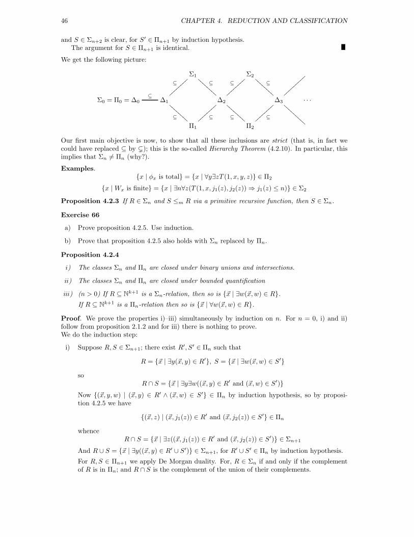
46 CHAPTER 4. REDUCTION AND CLASSIFICATION
and S ∈ Σn+2 is clear, for S′ ∈ Πn+1 by induction hypothesis.The argument for S ∈ Πn+1 is identical.
We get the following picture:
Σ1
⊆
BBBB
BBBB
Σ2
⊆
BBBB
BBBB
Σ0 = Π0 = ∆0⊆
∆1
⊆||||||||
⊆ BBBB
BBBB
∆2
⊆||||||||
⊆ BBBB
BBBB
∆3
|||||||||
BBBB
BBBB
B. . .
Π1
⊆
||||||||
Π2
⊆
||||||||
Our first main objective is now, to show that all these inclusions are strict (that is, in fact wecould have replaced ⊆ by (); this is the so-called Hierarchy Theorem (4.2.10). In particular, thisimplies that Σn 6= Πn (why?).
Examples.{x | φx is total} = {x | ∀y∃zT (1, x, y, z)} ∈ Π2
{x | Wx is finite} = {x | ∃n∀z(T (1, x, j1(z), j2(z)) ⇒ j1(z) ≤ n)} ∈ Σ2
Proposition 4.2.3 If R ∈ Σn and S ≤m R via a primitive recursive function, then S ∈ Σn.
Exercise 66
a) Prove proposition 4.2.5. Use induction.
b) Prove that proposition 4.2.5 also holds with Σn replaced by Πn.
Proposition 4.2.4
i) The classes Σn and Πn are closed under binary unions and intersections.
ii) The classes Σn and Πn are closed under bounded quantification
iii) (n > 0) If R ⊆ Nk+1 is a Σn-relation, then so is {~x | ∃w(~x,w) ∈ R}.
If R ⊆ Nk+1 is a Πn-relation then so is {~x | ∀w(~x,w) ∈ R}.
Proof. We prove the properties i)–iii) simultaneously by induction on n. For n = 0, i) and ii)follow from proposition 2.1.2 and for iii) there is nothing to prove.We do the induction step:
i) Suppose R,S ∈ Σn+1; there exist R′, S′ ∈ Πn such that
R = {~x | ∃y(~x, y) ∈ R′}, S = {~x | ∃w(~x,w) ∈ S′}
soR ∩ S = {~x | ∃y∃w((~x, y) ∈ R′ and (~x,w) ∈ S′)}
Now {(~x, y, w) | (~x, y) ∈ R′ ∧ (~x,w) ∈ S′} ∈ Πn by induction hypothesis, so by proposi-tion 4.2.5 we have
{(~x, z) | (~x, j1(z)) ∈ R′ and (~x, j2(z)) ∈ S′} ∈ Πn
whenceR ∩ S = {~x | ∃z((~x, j1(z)) ∈ R′ and (~x, j2(z)) ∈ S′)} ∈ Σn+1
And R ∪ S = {~x | ∃y((~x, y) ∈ R′ ∪ S′)} ∈ Σn+1, for R′ ∪ S′ ∈ Πn by induction hypothesis.
For R,S ∈ Πn+1 we apply De Morgan duality. For, R ∈ Σn if and only if the complementof R is in Πn; and R ∩ S is the complement of the union of their complements.

4.2. THE ARITHMETICAL HIERARCHY 47
ii) Suppose R ∈ Σn+1. Then for some R′ ∈ Πn we have that R = {~x | ∃y(~x, y) ∈ R′}. It followsthat
{(~x, y) | ∀w ≤ y(~x,w) ∈ R} ={(~x, y) | ∀w ≤ y∃z(~x,w, z) ∈ R′} ={(~x, y) | ∃σ(lh(σ) = y + 1 and ∀i ≤ y(~x, i, (σ)i) ∈ R′)}
Now apply the induction hypothesis and proposition 4.2.5.
iii) Use coding of pairs and proposition 4.2.5:
{~x | ∃y∃w(~x, y, w) ∈ R} = {~x | ∃y(~x, j1(y), j2(y)) ∈ R}
Proposition 4.2.5 Let n > 0. Then proposition 4.2.3 also holds without the restriction to re-ducibility via primitive recursive functions: if S ∈ Σn and R ≤m S, then R ∈ Σn.
Exercise 67
i) Prove proposition 4.2.5. Hint: if R ≤m S via φf , then the statement “x ∈ R” is equivalentto both of the following statements:
∃y (T (1, f, x, y) ∧ U(y) ∈ S)∀y(T (1, f, x, y) → U(y) ∈ S)
ii) Show that the proposition also holds with Σn replaced by Πn or ∆n.
iii) Why is the condition n > 0 necessary?
In order to find some n for which a given relation is in Σn or Πn, we apply the so-called Tarski-Kuratowski algorithm: first write R as a combination of primitive recursive relations, using thelogical symbols ∧,∨,¬,→, ∃, ∀. Then move the quantifiers to the front of the definition using thefamiliar logical laws:
i) ¬∀xφ↔ ∃x¬φ¬∃xφ↔ ∀x¬φ
ii) (∀xφ) ∧ ψ ↔ ∀x(φ ∧ ψ)(∀xφ) ∨ ψ ↔ ∀x(φ ∨ ψ)if the variable x does not occur in ψ; similarly for ∃;
iii) ((∀xφ) → ψ) ↔ ∃x(φ→ ψ)((∃xφ) → ψ) ↔ ∀x(φ→ ψ)if x does not occur in ψ.
The conditions in ii) and iii) make it sometimes necessary to “rename bound variables” (i.e., write∀yφ(y) instead of ∀xφ(x)). The result is what logicians call a prenex normal form: all quantifiersare at the front. Now one can say:
if the formula starts with ∃ and there are n quantifier alternations, the relation is Σn+1;
if the formula starts with ∀ and there are n quantifier alternations, the relation is Πn+1;
if the formula is quantifier-free, the relation is Σ0.
Example. Let R = {x | φx is total and bounded} =
= {x | ∀y∃zT (1, x, y, z)∧ ∃n∀y∀z(T (1, x, y, z) → U(z) ≤ n)}= (rename bound variables)
{x | ∀y∃zT (1, x, y, z)∧ ∃n∀v∀w(T (1, x, v, w) → U(w) ≤ n)}= {x | ∀y∃z(T (1, x, y, z)∧ ∃n∀v∀w(· · · ))}= {x | ∀y∃z∃n∀v∀w(· · · )}
48 CHAPTER 4. REDUCTION AND CLASSIFICATION
with (· · · ) primitive recursive; so R is a Π3-relation. But after renaming the bound variables, wecould also have started by moving the quantifiers from the second part to the front. Then we get:
{x | ∃n∀v∀w∀y∃z(· · · )}
and we conclude that R is also a Σ3-relation. We see that this R is a ∆3-relation.The Tarski-Kuratowski algorithm always gives us some n such that our relation is Σn or Πn
(provided our relation can be defined in logical terms), but seldom the most ‘economical’; and itdoes not tell us anything about ∆n-relations (as in the example).In order to prove that a given relation R (about which one knows, for example, that it is a∆n+1-relation) is not Σn or Πn, the algorithm offers no help, and we have to get to work.
Example 4.2.6 The relation R = {x | φx is total and bounded} is not a Π2-relation.
Proof. Suppose for a contradiction that R ∈ Π2. Then we would have for some primitive recursiverelation S(x, y, z):
φx is total and bounded ↔ ∀y∃zS(x, y, z)
Using the Recursion Theorem, pick an index e satisfying, for all y:
e·y ≃ max({w ≤ y | ∀v ≤ w∃z ≤ yS(e, v, z)})
where, by convention, max(∅) = 0. Then φe is total. However, by choice of e one can check that
φe is bounded ↔ ∃y∀z¬S(e, y, z)
On the other hand, from the assumed property of S it follows that
∃y∀z¬S(e, y, z) ↔ φe is not total and bounded
hence, we have obtained the desired contradiction.
Exercise 68 Prove that {x | φx is total and bounded} is also not Σ2.[Hint: the definition of “total and bounded” consists of a Σ2-part and a Π2-part. In the Example,in order to prove that the relation is not Π2, the Σ2-part is exploited. In this exercise, you mustwork with the Π2-component]
The given example shows us, that the inclusions Π2 ⊆ ∆3 and Σ2 ⊆ ∆3 are strict. We shall nowsee that all inclusions Πn ⊆ ∆n+1, Σn ⊆ ∆n+1, ∆n ⊆ Σn, ∆n ⊆ Πn are strict.
Definition 4.2.7 Define for all n, k ≥ 1 a Σn-relation E(k)n ⊆ Nk+1 as follows:
E(k)n = {(z, x1, . . . , xk) | ∃y1∀y2 · · · ∃ynT (n+ k − 1, z, jn+k−1(x1, . . . , xk, y1, . . . , yn−1), yn)}
if n is odd, and
E(k)n = {(z, x1, . . . , xk) | ∃y1∀y2 · · · ∀yn¬T (n+ k − 1, z, jn+k−1(x1, . . . , xk, y1, . . . , yn−1), yn)}
if n is even.
Theorem 4.2.8 (Kleene Normal Form Theorem) Let n > 0.For every Σn-relation R ⊆ Nk there is a number z such that
R = {~x ∈ Nk | (z, ~x) ∈ E(k)n }
and for every Πn-relation S ⊆ Nk there is a z such that
S = {~x ∈ Nk | (z, ~x) 6∈ E(k)n }
4.2. THE ARITHMETICAL HIERARCHY 49
If R ⊆ Nk is a Σn-relation, then the representation of R as {~x | (z, ~x) ∈ E(k)n } is called a Σn-normal
form of R, and z is a Σn-index for R. Analogously, we have Πn-normal forms and indices.
Proof. The statement about the Πn-relations follows immediately from the one about Σn-relations. We prove this one by induction on n ≥ 1:
Every Σ1-relation isW(k)e for a certain e; in other words, it can be written as {~x | ∃yT (k, e, jk(~x), y)}.
Suppose R is a Σn+1-relation. Then R = {~x | ∃yS(~x, y)} for some Πn-relation S ⊆ Nk+1; hence
Nk+1 − S is Σn and by induction hypothesis we have (~x, y) 6∈ S ↔ (z, ~x, y) ∈ E(k+1)n for some z.
Now assume that n is odd (the other case is proved in the same way). We get:
~x ∈ R ↔
∃y[(z, ~x, y) 6∈ E(k+1)n ] ↔
∃y¬∃y1∀y2 · · · ∃ynT (k + n, z, jk+n(~x, y, y1, . . . , yn−1), yn) ↔∃y∀y1 · · · ∀yn¬T (k + n, z, jk+n(~x, y, y1, . . . , yn−1), yn) ↔
(z, ~x) ∈ E(k)n+1
Proposition 4.2.9 The relation E(k)n is Σn but not Πn.
Proof. We do this for k = 1. Suppose E(1)n ∈ Πn, then also {x | (x, x) ∈ E
(1)n } ∈ Πn, and by the
Normal Form Theorem there is a z such that for all x:
(x, x) ∈ E(1)n if and only if (z, x) 6∈ E(1)
n
But of course, this yields a contradiction for x = z.
Corollary 4.2.10 (Hierarchy Theorem) All inclusions in the arithmetical hierarchy are strict.
Proof. Indeed, the fact that E(k)n ∈ Σn − Πn implies that ∆n ( Σn and that Πn ( ∆n+1. And
from the fact that Nk+1 − E(k)n ) ∈ Πn − Σn it follows that ∆n ( Πn and Σn ( ∆n+1.
Exercise 69 Prove: if R is m-complete in Σn, then R 6∈ Πn.
Exercise 70 Prove: if A is m-complete in Σn and B is m-complete in Πn, then A ⊔B ∈ ∆n+1 \Σn ∪ Πn.
Proposition 4.2.11 The relations E(k)n are m-complete in Σn en their complements are therefore
m-complete in Πn.
Proof. This is immediate from the Normal Form Theorem (4.2.8).
The classification of a set X ⊆ Nk is determining its exact position in the arithmetical hierarchy.A straightforward way to proceed is as follows: by the Tarski-Kuratowski algorithm one tries tofind a smallest possible n such that X ∈ Σn or Πn of ∆n. If one knows that X ∈ Σn and doesn’t
succeed in proving that X ∈ Πn, then one tries to prove that for appropriate k, E(k)n ≤m X holds.
Example 4.2.12 The set {x | φx is total} is strictly Π2.
Proof. Let us call this set Tot. We shall show that N2 − (E(1)2 ) ≤m X .
Recall that N2 − (E(1)2 ) = {(z, x) | ∀y1∃y2T (2, z, j(x, y1), y2)}. Let g be an index which satisfies
for all z, x, y1:
g·(z, x, y1) ≃ z·(x, y1)
50 CHAPTER 4. REDUCTION AND CLASSIFICATION
We now have:(w1, w2) 6∈ E
(1)2 if and only if
∀y1∃y2T (2, w1, j(w2, y1), y2) if and only if∀y1∃y2T (1, S2
1(g, w1, w2), y1, y2) if and only ifφS2
1(g,w1,w2) is total
Dus N2 − (E(1)2 ) ≤m X , as desired.
Exercise 71 Show that {e |We is a singleton set} is strictly ∆2.
Exercise 72 Find for each of the following relations an n, as small as you can, such that theyare in Σn, Πn or ∆n:
i) {e |We is finite}
ii) {e | rge(φe) is infinite}
iii) {e | φe is constant (possibly partial)} = {e | φe has at most one value}
iv) {j(e, f) |We ≤m Wf}
v) {e |We is m-complete in Σ1}
Then, classify the first three of these completely, by showing that they are m-complete in the classyou found.
4.2.1 Some exact classifications
In this section I treat two examples of exact classifications, which are not so immediate. Thereis extensive theory about obtaining such classifications: see [38]. However, this goes beyond thescope of this course. Therefore, the classifications below are done with “bare hands”.
Functions with no total extension
Our first example is the set
X = {x | φx cannot be extended to a total recursive function}
By exercise 51, the set X is nonempty.
Exercise 73 Prove that X is not Σ1:
a) using the Myhill-Shepherdson Theorem (3.3.3)
b) without using the Myhill-Shepherdson Theorem
By the Tarski-Kuratowski algorithm we easily find out that X is a Π3-set: we have that e ∈ X ifand only if the following condition holds:
∀f(if φf is total then φe is not a subfunction of φf )
We can rewrite this as
∀f(∀x∃yT (1, f, x, y) → ∃uvw(T (1, e, u, v) ∧ T (1, f, u, w) ∧ U(v) 6= U(w)))
which we bring in prenex normal form:
∀f∃uvwx∀y(T (1, f, x, y) → (T (1, e, u, v) ∧ T (1, f, u, w) ∧ U(v) 6= U(w)))
hence X ∈ Π3.
4.2. THE ARITHMETICAL HIERARCHY 51
Proposition 4.2.13 X is m-complete in Π3.
Proof. Let A be an arbitrary Π3-set:
A = {f | ∀x∃y∀zR(f, x, y, z)}
where R is some primitive recursive predicate. We have to find a total recursive function G suchthat A = G−1(X).By the Smn-theorem there is a primitive recursive function G such that for all f and z, G(f)·z isgiven by the following instructions:
Find the least W such that either (1) or (2) below holds:
1) ∃x ≤ j1(z)∀y ≤ j2(z)∃w ≤W¬R(f, x, y, w)
2) ∀y ≤ j2(z)∃w ≤WT (1, j1(z), j(j1(z), y), w)
Let G(f)·z be undefined if such a W is not found.
If W has been found, put G(f)·z = W if (1) holds.
If (1) does not hold, find the least w satisfying T (1, j1(z), z, w), and put G(f)·z =U(w) + 1.
Now suppose f ∈ A so ∀x∃y∀zR(f, x, y, z), and suppose φu is a total function.For every x let nx = max({m | ∀y < m∃z¬R(f, x, y, z)}); and define
N(u) = max({nx | x ≤ u}) + 1
Then G(f)·j(u,N(u)) is always defined (the required W is always found by (2), because φu istotal), but the obtained W can never satisfy (1) (check this yourself); so G(f)·j(u,N(u)) =u·j(u,N(u)) + 1, and therefore φu is not a total function which extends φG(f). This holds forevery index u such that φu is total, and hence G(f) ∈ X .
If f 6∈ A then ∃x∀y∃z¬R(f, x, y, z); let N be minimal such that ∀y∃z¬R(f,N, y, z). Then wehave:
If j1(z) ≥ N , then G(f)·z is defined (the required W will be found because (1) will occur).
If j1(z) < N then the partial function φG(f) depends on j1(z):
The function λn.G(f)·j(j1(z), n) is total if the function λx.j1(z)·j(j1(z), x) is total, and hasfinite domain if λx.j1(z)·j(j1(z), x) is not total. In both cases, the function λn.G(f)·j(j1(z), n)has a total recursive extension Fj1(z).
Now define
H(z) =
F0(j2(z)) if j1(z) = 0...
...FN−1(j2(z)) if j1(z) = N − 1G(f)·z otherwise
Then H is a total recursive function which extends φG(f).
Primitive recursive functions
Our second example is the set
PRIM = {e |φe is primitive recursive}
Proposition 4.2.14 The set PRIM is strictly ∆3.

52 CHAPTER 4. REDUCTION AND CLASSIFICATION
Proof. In the proof of 2.1.11 we have defined codes for definitions of primitive recursive functions.From this definition it is not hard to see, that the set of such codes, let’s call it C, is recursive (infact, primitive recursive).
Moreover, since the partial recursive functions are closed under double recursion (2.4.7), thereis a partial recursive function ψ such that for all n ∈ C and m arbitrary, ψ(n,m) = Fn(m), whereFn denotes the primitive recursive function whose definition is coded by n.
Define a total recursive function E as follows:
E(n,m) =
{0 if n 6∈ C
Fn(m) + 1 if n ∈ C
Now we can write the set PRIM as intersection:
PRIM =
{e |φe is total}∩
{e | ∃n∀m∀k(T (1, e,m, k) → E(n,m) = U(k) + 1)}
We see that PRIM is the intersection of a Π2-set and a Σ2-set. Hence, by proposition 4.2.4, PRIMis in ∆3 (check!). We need to show that PRIM is neither a Σ2, nor a Πs-set.
We show that PRIM is not Σ2 by showing that every Π2-set is many-one reducible to PRIM. LetA be an arbitrary Π2-set, so A = {e | ∀x∃yR(e, x, y)} with R recursive. Choose an index g suchthat
g·(e, x) ≃
{0 if ∃yR(e, x, y)
undefined otherwise
Then clearly, since the function φS11(g,e) is constant 0 on its domain, it is primitive recursive if and
only if it is total. Hence we have: S11(g, e) ∈ PRIM if and only if ∀x∃yR(e, x, y), in other words:
if and only if e ∈ A. So the function e 7→ S11(g, e) reduces A to PRIM.
Similarly, we show that PRIM is not Π2 by showing that every Σ2-set is many-one reducible toPRIM. We use the recursive function ψ(n,m) = Fn(m) from above. Suppose A = {e | ∃x∀yR(e, x, y)}with R recursive.
Let, for any number n, M(n) be the least m ≤ n such that for all k ≤ n, R(e,m, k) holds.Of course, M(n) need not exist, but this can be decided recursively. Let g be an index of thefollowing total recursive function:
φg(e, n) =
0 if n = 00 if n > 0, M(n) and M(n− 1) both
exist, and M(n) = M(n− 1)Fk(n) + 1 otherwise, where k is such that n is
the k + 1-st number for which the first clause fails
Now suppose e ∈ A. Let N be the least number such that ∀yR(e,N, y). Then for all i < N thereis a least number yi such that ¬R(e, i, yi). Therefore if m > max{yi | i < N} + 1, then alwaysM(m) = M(m−1) will hold, so φg(e,m) = 0. We see that φS1
1(g,e)(m) will be 0 for all but finitely
many m, hence φS11(g,e) is primitive recursive: S1
1(g, e) ∈ PRIM.Conversely, suppose e 6∈ A. Then the first clause in the definition og φg(e, n) will fail infinitely
often. Tha means that for all k there will be an n such that φS11(g,e)(n) differs from Fk(n).
Therefore φS11(g,e) cannot be primitive recursive. We conclude that the function e 7→ S1
1(g, e)
reduces A to PRIM, as desired.
4.3 R.e. sets again: recursive, m-complete, and in-between
In this section we shall see that the concept of many-one reducibility gives a nontrivial structureon the class of all r.e. sets.
4.3. R.E. SETS AGAIN: RECURSIVE, M -COMPLETE, AND IN-BETWEEN 53
First we consider r.e. sets which are extensional for indices of r.e. sets (see section 3.3). Thesesets will turn out to be either recursive or m-complete in Σ1.
Then we characterize the m-complete r.e. sets: these are “recursively isomorphic” to K, thestandard set. Moreover, they are precisely the creative sets (see Exercise 52): this is Corollary 4.3.6below.
Finally we show that there exist r.e. sets which are neither recursive, nor m-complete. Thestructure of the preordered set (RE ,≤m) is quite complicated, and topic of ongoing research.
4.3.1 Extensional r.e. sets
Exercise 74 Show the following corollary of Rice’s Theorem: if X ⊆ N is recursive and exten-sional for indices of r.e. sets, then X = ∅ or X = N.
Proposition 4.3.1 If X ⊆ N is r.e. and extensional for indices of r.e. sets, then X is eitherrecursive, or m-complete in Σ1.
Proof. Suppose X satisfies the assumptions of the proposition, and suppose also that X 6= ∅,X 6= N. Then by Exercise 74 we have that X is not recursive, so we show that X is m-completein Σ1.
The Rice-Shapiro Theorem implies that if n ∈ X for some n such that Wn = ∅, then X = N.So we may assume that indices for the empty set are not elements of X . On the other hand wehave assumed X nonempty; choose e ∈ X . Let g ∈ N be arbitrary.
By the Smn-theorem there exists a primitive recursive function F satisfying for all x, y:
F (x)·y ≃ µz.[T (1, e, y, j1(z)) ∧ T (1, g, x, j2(z))]
Then the following holds:
WF (x) =
{We if x ∈Wg
∅ otherwise
In other words, by the assumptions on X we have for all x: x ∈ Wg if and only if F (x) ∈ X . SoWg ≤m X via F , and since g was arbitrary we have proved that X is m-complete in Σ1.
4.3.2 m-Complete r.e. sets
We recall from Exercise 52: a set X ⊆ N is called creative if X is r.e. and there is a partialrecursive function ψ with the following property:
Whenever We ∩X = ∅ then ψ(e) is defined and ψ(e) 6∈We ∪X
(X is said to be creative via ψ)
Exercise 75 Prove that K is creative.
In this section we shall show that an r.e. set is m-complete precisely when it is creative.
Definition 4.3.2 By the notation X ≤1 Y we mean that X is many-one reducible to Y via aninjective total recursive function. We say X is 1-complete in a class of sets, if for every set Y inthat class we have Y ≤1 X .
We call subsets X,Y of N recursively isomorphic if there is a total recursive bijective functionh : N → N with h[X ] = Y .
The following theorem is sometimes called the “recursive analogue of the Cantor-Bernstein Theo-rem” (in set theory, the Cantor-Bernstein Theorem says that whenever there are injective functionsX → Y and Y → X , there is also a bijection from X to Y ).
Theorem 4.3.3 (Myhill’s Isomorphism Theorem) For any two sets A,B ⊆ N we have: ifA ≤1 B and B ≤1 A then A and B are recursively isomorphic.
54 CHAPTER 4. REDUCTION AND CLASSIFICATION
Proof. Suppose A ≤1 B via f and B ≤1 A via g, so f and g are total recursive injective functionssatisfying A = f−1(B) and B = g−1(A). We now construct, by primitive recursion, a sequence(hs)s≥0 of coded sequences, such that for every i < k < lh(hs) we have: if j1((hs)i) = j1((hs)i′ )then (hs)i = (hs)i′ , and j2((hs)i) = j2((hs)i′) then (hs)i = (hs)i′ . We can therefore think of thesequences hs as graphs of finite injective functions; we shall use the notation hs also to denotethese functions. Note, that we can recursively from hs, obtain its domain, range and inverse:
x ∈ dom(hs) if and only if ∃i < lh(hs) j1((hs)i) = xx ∈ rge(hs) if and only if ∃i < lh(hs) j2((hs)i) = x
(hs)−1(y) = µx < hs.∃i < lh(hs) (hs)i = j(x, y)
In the end, the finite injective functions hs will be pieced together to form a bijection h : N → N.
Let h0 be the code of the empty sequence. Now suppose hs is given, such that hs is the graph ofa finite injective function, and for every x ∈ dom(hs) we have x ∈ A if and only if hs(x) ∈ B.
If s+1 = 2x+1 we define h(x). If already x ∈ dom(hs) we put hs+1 = hs. Otherwise, we computethe sequence f(x), f(h−1
s (f(x))), . . . , f(h−1s f)n(x), . . ., until the first element y is found which
satisfies y 6∈ rge(hs). Such a y must exist because f and hs are injective and x 6∈ dom(hs). Puths+1 = hs∗〈j(x, y)〉. Check yourself that hs+1 is still injective and still satisfies for n ∈ dom(hs+1):n ∈ A if and only if hs+1(n) ∈ B.
If s+ 1 = 2x+ 2, we define h−1(x). This is done in the same way, with f, hs, dom en rge replacedby (respectively) g, h−1
s , rge en dom.
Proposition 4.3.4 If a set X is creative, then there is an injective total recursive function Psuch that X is creative via P .
Proof. Let X be creative via φ. Check that there is a primitive recursive function G is satisfying
WG(x) =
{Wx if φ(x) is defined∅ otherwise
Define Q by: Q(x) = φ(x) or Q(x) = φ(G(x)), whichever computation terminates first. Then thefunction Q is total, for if φ(x) is undefined, then WG(x) = ∅, hence φ(G(x)) is defined because Xis creative via φ.
We also have that if Wx ∩ X = ∅ then φ(x) is defined, hence Wx = WG(x), so in this caseφ(x) 6∈ X ∪Wx and φ(G(x)) 6∈ X ∪Wx. This means that X is also creative via Q, and Q is total.It remains to modify Q to an injective function P .
Let H be a primitive recursive function satisfying for all x:
WH(x) = Wx ∪ {Q(x)}
It now folows that:WHn+1(x) = Wx ∪ {Q(x), QH(x), . . . , QHn(x)}
Define the function P as follows:
- P (0) = Q(0)
- Suppose P (0), . . . , P (x) have been defined. Now enumerate the sequence Q(x+ 1), QH(x+1), . . . , QHn(x + 1), . . ., until a) or b) occurs:
a) For some n, QHn(x+ 1) 6∈ {P (0), . . . , P (x)}. Put P (x+ 1) = QHn(x+ 1).
b) A repitition occurs: for some n, we have QHn+1(x + 1) ∈ {Q(x + 1), . . . , QHn(x +1)}. Then we must have Wx+1 ∩ X 6= ∅ (check); simply let P (x + 1) = µy.[y 6∈{P (0), . . . , P (x)}].
Convince yourself that P is injective and total, and that X is creative via P .
4.3. R.E. SETS AGAIN: RECURSIVE, M -COMPLETE, AND IN-BETWEEN 55
Proposition 4.3.5 (Myhill) If a set X is creative, then K ≤1 X
Proof. Choose (by proposition 4.3.4) an injective and total recursive function P such that X iscreative via P . Let F be a primitive recursive function satisfying
WF (x,y) =
{{P (x)} if y ∈ K∅ otherwise
By the Recursion Theorem, there is a primitive recursive, injective function N satisfying for all y:
WN(y) = WF (N(y),y) =
{{P (N(y))} if y ∈ K∅ otherwise
(Choose by the Recursion Theorem an n such that for all y, x, n·(y, x) ≃ F (S11(n, y), y)·x. Let
N(y) = S11(n, y). Then WN(y) = WF (N(y),y) and N can be assumed to be injective because it is
an Smn-function (Exercise 29))The following hold:
If y ∈ K then WN(y) = {P (N(y))} hence WN(y) ∩X 6= ∅ hence P (N(y)) ∈ X
If y 6∈ K then WN(y) = ∅ hence WN(y) ∩X = ∅ hence P (N(y)) 6∈ X
so we conclude that K ≤1 X via the composition PN .
Exercise 76 Prove:
i) If X is creative then X is strictly r.e.
ii) If X is creative, then there is an infinite r.e. set which is disjoint from X
iii) If X is creative and Y is r.e. and X ≤m Y , then Y is creative
Corollary 4.3.6 For a set X ⊆ N the following assertions are equivalent:
i) X is creative
ii) X is 1-complete in Σ1;
iii) X is m-complete in Σ1;
iv) There is a total recursive bijective function h such that h[X ] = K
Exercise 77 Prove Corollary 4.3.6. Hint: first prove that K is 1-complete in Σ1. Use Exercise 76,proposition 4.3.5 and Theorem 4.3.3.
Exercise 78 Call a disjoint pair (A,B) of r.e. sets effectively inseparable if there exists a partialrecursive function ψ which is such that for all x and y: if A ⊆Wx and B ⊆Wy and Wx ∩Wy = ∅,then ψ(〈x, y〉) is defined and ψ(〈x, y〉) 6∈ Wx ∪Wy.
a) Show: we may assume that ψ is total and injective.
b) Show: the sets A = {x | x·x = 0} and B = {x | x·x = 1} are effectively inseparable.
c) Show: if (A,B) is effectively inseparable then A and B are creative.
Exercise 79 Show that there exist disjoint r.e. sets A,B ⊆ N such that (A,B) is recursivelyinseparable, but not effectively inseparable.

56 CHAPTER 4. REDUCTION AND CLASSIFICATION
4.3.3 Simple r.e. sets: neither recursive, nor m-complete
Definition 4.3.7 An r.e. set A is called simple if N−A is infinite but does not contain an infiniter.e. subset (in other words: A intersects every infinite r.e. set).
Exercise 80 Show: if A is a simple r.e. set, then A is neither recursive, nor creative.
Since we know from Corollary 4.3.6 that the m-complete sets are precisely the creative sets, itsuffices for us to show that simple sets exist.
Theorem 4.3.8 (Post, 1944) There exists a simple set.
Proof. Definne the partial recursive function ψ by:
ψ(e) ≃ j1(µz.[T (1, e, j1z, j2z) ∧ j1z > 2e])
Let S = rge(ψ). Then S is certainly r.e. Because always ψ(e) > 2e (if ψ(e) is defined), the set Scontains, for each e, at most e elements from the set {0, 1, . . . , 2e}; and therefore the set N − S isinfinite.Moreover, if B = We is an infinite r.e. set, then ψ(e) is defined, and ψ(e) ∈ S ∩We (check this!).So S intersects every infinite r.e. set. This implies that N − S, being infinite and disjoint from S,cannot be r.e.; so S is not recursive.We conclude that S is simple, as claimed.
4.3.4 Non-Arithmetical Sets; Tarski’s Theorem
In section 2.1.2 we introduced the language of ordered rings, also called the language of arithmeticby logicians. We formulated the theory IΣ1 in this language, and stated that for every k-aryprimitive recursive function F there is a formula φ(x1, . . . , xk+1) in the language, such that thesentences:
ψ(n1, . . . , nk, F (n1, . . . , nk)) for all n1, . . . , nk∀~xyz (ψ(~x, y) ∧ ψ(~x, z) → y = z)
∀~x∃yψ(~x, y)
are all consequences of IΣ1 (i.e., true in every model of IΣ1).This means, that for every set A ⊆ Nk in the Arithmetical Hierarchy, there is a formula
ψA(x1, . . . , xk) in the language of arithmetic, such that for every k-tuple n1, . . . , nk of naturalnumbers the following holds:
(n1, . . . , nk) ∈ A ⇔ N |= ψA(n1, . . . , nk)
where N is the obvious structure for the language of arithmetic.In the course of proving his famous Incompleteness Theorems, Godel constructed a coding of
formulas of the arithmetical language; assigning to every formula ϕ a number pϕq. This codingwas done in such a way that he was able to prove the following lemma (we present a simplifiedversion):
Lemma 4.3.9 (Diagonalization Lemma; Godel, 1930) For every formula ϕ(x) in one freevariable x there exists a sentence ψ such that the sentence
ψ ↔ ϕ(pψq)
is a consequence of IΣ1.
The logician Alfred Tarski extracted the following consequence of this lemma:
Theorem 4.3.10 (Tarski’s Theorem, 1936) The set
T = {pψq |ψ is an arithmetical sentence such that N |= ψ}
is not arithmetical (i.e., does not belong to the Arithmetical Hierarchy).
4.3. R.E. SETS AGAIN: RECURSIVE, M -COMPLETE, AND IN-BETWEEN 57
Proof. Suppose T were arithmetical. Then there would be a formula χT (x) in one variable, suchthat for any number n we would have: n ∈ T if and only if χT (n) is true in the model N.
But now apply the Diagonalization Lemma 4.3.9 to the formula ¬χT . We obtain a sentenceψ such that the equivalence ψ ↔ ¬χT (pψq) is a consequence of IΣ1, and therefore true in N. Weobtain:
N |= ψ ⇔pψq ∈ T ⇔N |= χT (pψq) ⇔N |= ¬ψ
which is a clear contradiction.
58 CHAPTER 4. REDUCTION AND CLASSIFICATION

Chapter 5
Relative Computability and
Turing Reducibility
The stratification of subsets of N in ≡m-classes was important because of the close connectionwith the Arithmetical Hierarchy.
However, for other important issues in Computability Theory we need a different type ofreduction. The question we shall deal with in this chapter is: which functions are computable, ifa certain function F is “given” to me as computable, for example by some infinite database?
In other words, which functions can be computed partial-recursively from F?
5.1 Functions partial recursive in F
Definition 5.1.1 The class of functions primitive recursive in a given function F is the least classof functions which contains the basic functions from Definition 2.1.1, as well as F , and is closedunder definition by composition and primitive recursion.
Exercise 81 Show that the function λx.FF (0)(x) is primitive recursive in F .
Definition 5.1.2 The class of functions partial recursive in F is defined as in Definition 2.2.1,with ‘primitive recursive’ replaced by ‘primitive recursive in F ’.
We can also introduce the notion ‘computable in F ’, by extending the concept of Register Machine.We now think of a machine which is able to produce the values of F in a ‘magical’ way, whichexplains the name “oracle” in the next definition.
Definition 5.1.3 The programming language for the Register Machine with oracle F has, inaddition to the commands r+i ⇒ j and r−i ⇒ j, k of section 1.1, also commands of the form
ri = F (rj) ⇒ k
which are read as follows: replace the content of the i-th register by F (rj) (leaving all otherregister contents unchanged) and move to the k-th command.
If we code the command ri = F (rj) ⇒ k by 〈i, j, k, 0〉 then we can rewrite section 2.4 as follows:
There is a primitive recursive set Prog′ of codes of programs for the RM with oracle: e ∈ Prog′
if and only if
lh(e) > 0 ∧ ∀i < lh(e)[lh((e)i) ∈ {2, 3} ∨ (lh((e)i) = 4 ∧ ((e)i)3 = 0)]
By φFm,e we denote the m-ary partial function which is computed by the program with codee and with oracle F .
59
60 CHAPTER 5. RELATIVE COMPUTABILITY AND TURING REDUCIBILITY
There is a ternary partial function ΦF defined by
ΦF (m, e, x) ≃
{undefined if ¬Prog′(e)φFm,e(j
m1 (x), . . . , jmm(x)) otherwise
In full analogy to 2.3.1 we have:
Proposition 5.1.4 ΦF is partial recursive in F . Moreover, for every k-ary partial function Gwhich is partial recursive in F there is a number e such that
G(x1, . . . , xk) ≃ ΦF (k, e, jk(x1, . . . , xk))
for all x1, . . . , xk.
The proof constructs a relation TF (m, e, jm(x1, . . . , xm), y) which holds if and only if y codes acomputation on the RM with oracle F , with a program with code e and input x1, . . . , xm.
The relation TF is not simply primitive recursive, but primitive recursive in F , because inorder to check whether it holds, we must verify that the commands ri = F (rj) ⇒ k have beencorrectly executed.
The output function U(y) = ((y)lh(y)−1)1 remains the same, and is primitive recursive.
Corollary 5.1.5 The class of partial functions of the form φFm,e coincides with the class of func-tions partial recursive in F .
We also have the Smn-theorem and the Recursion Theorem in this more general context:
Proposition 5.1.6 (Smn-theorem) There are primitive recursive functions Smn , satisfying
φFn,Smn (e,x1,...,xm)(y1, . . . , yn) ≃ φFm+n,e(x1, . . . , xm, y1, . . . , yn)
Proposition 5.1.7 (Recursion Theorem, primitive-recursively uniform version) There ex-ists a primitive recursive function T satisfying, for all f and x1, . . . , xm:
φFm,T (f)(x1, . . . , xm) ≃ φFm+1,f (x1, . . . , xm, T (f))
The reason that the functions Smn (and the function T in the Recursion Theorem) are primitiverecursive (you might have expected: primitive recursive in F ) is that they manipulate codes ofprograms and don’t act on computations; and the code for a program for the RM with oracleF does not depend on F . And the function T in the Recursion Theorem is a composition ofSmn-functions (see the proof of theorem 2.4.3).
Exercise 82 Use the fact (which is known as the Use Principle) that every computation ofφFm,e(x1, . . . , xm) uses only finitely many values of F , in order to show that the partial function
Φe,x1,...,xm: NN → N
defined by Φe,x1,...,xm(F ) ≃ φFm,e(x1, . . . , xm), is continuous on its domain (where we give NN the
same topology as in section 3.3).
When one defines functions partial recursive in F one writes the same sort of equations as withordinary partial recursive functions; the only difference is that one can use F as if it were recursive.
The following consideration is also useful: define the relation
T σ(m, e, jm(x1, . . . , xm), y)
as: y codes a computation “with oracle σ” for a coded finite sequence σ; that is, every time acommand ri = F (rj) appears we have rj < lh(σ) and ri is replaced by (σ)rj
.This relation is of course primitive recursive. Now in any computation on the RM with oracle
F we can separate the partial recursive part from the oracle:
5.2. SETS R.E. IN F ; THE JUMP OPERATION 61
Proposition 5.1.8 The statement φFm,e(x1, . . . , xm) = y is equivalent to the statement
∃σ[∀i < lh(σ)(σ)i = F (i) ∧ ∃w(T σ(m, e, jm(x1, . . . , xm), w) ∧ U(w) = y)]
So apart from the quantifier ∃σ we have a conjunction of something primitive recursive in F andsomething recursively enumerable.
Definition 5.1.9 For total functions F and G we say that F is Turing reducible to G, and wewrite F ≤T G, if F is recursive in G. For subsets A and B of N (Nk) we say that A is Turingreducible to B (and write A ≤T B) if χA ≤T χB.
Exercise 83 Prove that the relation ≤T is a preorder on NN.
Exercise 84 Prove:If A ≤m B then A ≤T B
(N −A) ≤T AA ≤T B does not imply A ≤m B
Just as with ≤m, we can divide P(N) in ≡T -equivalence classes. The ≡T -class of a subset A ⊆ N
is called the degree of unsolvability (or Turing degree) of A.
Exercise 85 Prove that every pair A,B ⊆ N has a join w.r.t. ≤T .
Exercise 86 Prove that the following does not hold: if A ≤T B and B is r.e., then so is A.
Exercise 87 Given sets A and B, prove that the following assertions are equivalent:
i) B ≤T A
ii) There exist total recursive functions F and G such that the following holds:
x ∈ B if and only if ∃σ(σ ∈ WF (x) ∧ ∀i < lh(σ)(σ)i = χA(i))x 6∈ B if and only if ∃σ(σ ∈ WG(x) ∧ ∀i < lh(σ)(σ)i = χA(i))
(Hint: use proposition 5.1.8)
5.2 Sets r.e. in F ; the jump operation
Also a considerable part of Chapter 3 can be rewritten in the context of “recursive in F”. Inparticular, we have:
Proposition 5.2.1 Let KF = {e | φF1,e(e) is defined}. Then KF is not recursive in F .
The proof is analogous to the standard case.
Definition 5.2.2 A set A is called r.e. in F if A = dom(φF1,e) for some e (equivalently: one of theother conditions in proposition 3.2.2, suitably relativized to F ). The set A is called r.e. in B ⊆ N
if A is r.e. in χB.
Definition 5.2.3 For a set A, the set KχA is called the jump of A; we write A′ for this set.
The operation A 7→ A′ preserves ≡T -equivalence, as we shall see in proposition 5.2.4 below, andinduces therefore an operation on ≡T -equivalence classes. It is a tool for the study of the partialorder on Turing degrees.
Proposition 5.2.4 (Jump Theorem)
i) For every set A, A′ is r.e. in A
62 CHAPTER 5. RELATIVE COMPUTABILITY AND TURING REDUCIBILITY
ii) A′ is not recursive in A
iii) B r.e. in A if and only if B ≤m A′
iv) If A is r.e. in B and B ≤T C then A is r.e. in C
v) B ≤T A if and only if B′ ≤m A′
vi) A is r.e. in B if and only if A is r.e. in N −B
Proof. i) is evident.ii) This is proposition 5.2.1.iii) ‘Only if’ follows by a suitable relativization of the statement that K is m-complete in Σ1, and‘if’ follows from i) and the statement that if A is r.e. in C and B ≤m A, then B is r.e. in C.iv) If A is of the form {x | ∃yP (x, y)} with P recursive in B, then P is also recursive in C, so Ais r.e. in C.v) ‘Only if’ follows from iii), for B ≤T A implies that B′ is r.e. in A. For the ‘if’-direction,relativize proposition 3.2.5i) to: B ≤T A holds precisely if both B and N −B are r.e. in A. Fromiii) we can deduce that B ≤m B′ and (N−B) ≤m B′. We conclude: if B′ ≤m A′ then B is r.e. inA and N −B is r.e. in A, so B ≤T A.vi) This follows from Exercise 84.
Proposition 5.2.4 not only connects the notions ≤m and ≤T ; we also have as a direct consequenceof v) and Exercise 84 that B ≤T A implies B′ ≤T A′ (hence also: if B ≡T A then B′ ≡T A′).As stated before proposition 5.2.4, the mapping (−)′ is well-defined on Turing degrees, and isorder-preserving
We shall indicate Turing degrees by lower-case Greek letters: α, β, . . .The ≡T -class of ∅ is written O; this class consists precisely of the recursive sets. It is obvious
that O is the least element in the ordering of Turing degrees. The structure of the partial ordering of≡T -classes is quite complicated; much advanced Computability Theory (so-called Degree Theory)studies this partial order.
Exercise 88 Prove that K′ ∈ Σ2.
If we write A(n) for the n-fold jump of A, then the following holds in general: ∅(n) is m-completein Σn.
In the early 1940’s, E. Post whether every r.e. set is either recursive, or ≡T -equivalent to K; inother words, whether every r.e. set belongs to O ∪ O′.
For some time this was referred to as Post’s Problem. In 1956/57, Friedberg and Muchnikindependently answered this question in the negative: there exists an r.e. set A such that ∅ <TA <T K (here <T means: ≤T and 6≡T ). There also exist r.e. sets A and B whose degreesare incomparable w.r.t. ≤T . For such A and B we must then also have ∅ <T A <T K and∅ <T B <T K.
Exercise 89 Prove this last sentence.
Since we know that A ≤m B implies A ≤T B, this gives us another proof that there exist r.e.sets which are neither recursive, nor m-complete in Σ1. However, the Friedberg-Muchnik result issubstantially stronger (and harder) than Theorem 4.3.8.
We also conclude from the Friedberg-Muchnik result that there exist Turing degrees α which arenot of the form β′: the jump operation is not surjective.
We conclude this section with a theorem which says that the jump operation is surjective ondegrees ≥ O′:
Theorem 5.2.5 (Friedberg) Suppose β ≥ O′. Then there is an α satisfying α′ = α ⊔ O′ = β.
5.3. THE RELATIVIZED ARITHMETICAL HIERRARCHY 63
Proof. Choose B ∈ β. Because β ≥ O′ every r.e. set is recursive in B. We now define a B-recursive sequence of coded sequences (fs|s ∈ N), such that, whenever s ≤ t, then the sequencecoded by fs is an initial segment of the sequence coded by ft (which we denote by fs � ft). Thisis done as follows: f0 = 〈〉, the code of the empty sequence. Suppose fs has been defined.
- If s is even, s = 2e, determine whether
∃σ∃t[fs � σ ∧ T σ(1, e, e, t) ∧ ∀i < lh(σ)(σ)i ∈ {0, 1}] (∗)
If there exists a σ satisfying (∗), let fs+1 be the minimal such σ; otherwise, put fs+1 = fs.
- If s is odd, s = 2e+ 1, put fs+1 = fs ⋆ 〈χB(e)〉.
Observe that fs � fs+1 always holds and that the length of fs increases at every odd step, so thecollection of all fs determines a total function f (which takes values in {0, 1}).
Because condition (∗) is r.e. and therefore recursive in O′, hence recursive in B, and at oddsteps we use only χB, the resulting function f is recursive in B.
Let A = {x | f(x) = 0} and α the ≡T -class of A. Then A ≤T B, so the inequality α⊔O′ ≤T βis clear. We also always have α ⊔ O′ ≤T α′ (as you can check for yourself). Therefore, it remainsto show:
1) α′ ≤T β
2) β ≤T α ⊔ O′
For 1): in order to decide whether e ∈ A′ = {e | φA1,e(e) is defined}, determine whether (∗) holdsfor s = 2e. If (∗) holds, then there is a minimal 0-1 sequence σ such that f2e � σ and T σ(1, e, e, t)for some t; but then we have e ∈ A′ by definition.
If (∗) does not hold for s = 2e then clearly e 6∈ A′. Because condition (∗) is recursive in O′
and (fs)s≥0 is recursive in B, it follows that A′ ≤T B, hence α′ ≤ β.
For 2): χB(e) is the last element of the sequence coded by f2e+2, so B is recursive in the sequence(fs|s ∈ N).
Now f2e+1 is obtained recursively in O′ from f2e, and f2e+2 is obtained recursively in A fromf2e+1 (for f = χA, so f2e+2 = f2e+1 ⋆ 〈χA(lh(f2e+1))〉), so the enumeration (fs|s ∈ N) is recursivein A ⊔ ∅′, in other words B ≤T A ⊔ ∅′, so β ≤ α ⊔ O′.
5.3 The Relativized Arithmetical Hierrarchy
There are completely straightforward definitions of ΣFn , ΠFn : in the definition of Σn and Πn, replace
‘recursive’ by ‘recursive in F ’, and the T -predicate by TF .All theorems of section 4.2 generalize: we have Kleene Normaal Forms for ΣFn , which are
m-complete in ΣFn ; the hierarchy does not collapse.We call a set A arithmetical in F if A ∈
⋃
n∈NΣFn . We can represent the subsets of N which are
arithmetical in F , also in the following way: augment the language of arithmetic or ordered rings(see section 2.1.2) by a new function symbol F , and make the standard model N into a structurefor the new language by interpreting F as F . Again we have: A is arithmetical in F precisely ifthere exists a formula ϕ(x) in one free variable in the extended language, such that
A = {n ∈ N | N |= ϕ(n)}
One last exercise:
Exercise 90 Prove that for all n ≥ 1:
X ∈ ΣYn if and only if X ≤m Y (n)
Hint: use induction.
64 CHAPTER 5. RELATIVE COMPUTABILITY AND TURING REDUCIBILITY
Chapter 6
A Glimpse Beyond the
Arithmetical Hierarchy
In this final chapter of these notes, we shall have a look at sets which can be defined in “second-order logic”; that is, logic which has, in addition to variables for numbers (and quantifiers overthese variables) also variables and quantifiers for functions.
We have a hierarchy which extends the Arithmetical Hierarchy and which is called the Ana-lytical Hierarchy because traditionally, logicians refer to second order arithmetic as “analysis”.
6.1 Partial Recursive Functionals
We extend the concept of an RM with oracle of definition 5.1.3 to one with multiple oraclesF1, . . . , Fk: we have extra commands
ri = Fm(rj) ⇒ n (1 ≤ m ≤ k)
whose intended meaning is: replace ri by Fm(rj) and move to command n.We can code this command as 〈i, j, n, k〉 and again, we have a primitive recursive set of codes ofprograms, and we have partial functions
φF1,...,Fm
l,e (x1, . . . , xl)
which we call partial recursive in F1, . . . , Fm. This extension is completely straightforward; whatis new in this chapter is that we regard the expression φF1,...,Fm
l,e (x1, . . . , xl) as a partial functionalso of the variables F1, . . . , Fm.
Definition 6.1.1 A partial recursive k, l-ary functional is a partial function (NN)k × Nl → N ofthe form
(~F , ~x) 7→ φF1,...,Fk
l,e (x1, . . . , xl)
A partial recursive k, l-ary functional into NN is a partial function Φ : (NN)k ×Nl → NN such thatfor some partial recursive functional Ψ : (NN)k × Nl+1 → N we have:
a) Φ(~F , ~x) is defined if and only if for all y, Ψ(~F , ~x, y) is defined, and
b) If Φ(~F , ~x) is defined, then for all y we have
Φ(~F , ~x)(y) = Ψ(~F , ~x, y)
The word “functional” is often used for a function some of whose arguments are functions.Without developing an elaborate theory of these functionals, we state the following (which shouldbe intuitively clear) without proof:
65

66 CHAPTER 6. A GLIMPSE BEYOND THE ARITHMETICAL HIERARCHY
Proposition 6.1.2 The partial recursive functionals enjoy the following closure under composi-tion: if
Ψ1, . . . ,Ψk : (NN)m × Nn → NN
Φ1, . . . ,Φl : (NN)m × Nn → N
Ξ : (NN)k × Nl → N
are partial recursive functionals and Ψ1, . . . ,Ψk are total, then the map
(~F , ~x) 7→ Ξ(Ψ1(~F , ~x), . . . ,Ψk(~F , ~x),Φ1(~F , ~x), . . . ,Φl(~F , ~x))
is a partial recursive functional.
Example 6.1.3 Without the requirement that Ψ1, . . . ,Ψk be total in proposition 6.1.2, the resultis no longer true. The following example is instructive: let Φ be the partial recursive function
Φ(e, x) ≃
{0 if ∀y ≤ x¬T (1, e, e, y)
undefined otherwise
and let Ψ : N → NN be the partial recursive functional defined by Ψ(e) = λx.Φ(e, x). Note thatthe domain of Ψ is {e | e 6∈ K}, so if we compose Ψ with the (total) functional F 7→ F (0), we geta partial function N → N with domain N −K. This is not a partial recursive functional.
If we have an expression ϕ(~F , ~x) for a number or a function, we say that it is recursive in ~F , ~x if
it is the result of applying a partial recursive functional to ~F , ~x
Exercise 91 For a function F and number u, define Fu(x) = F (j(u, x)). Show that Fu is recursivein F, u.
For F, u let 〈u〉 ∗F be the function such that (〈u〉 ∗F )(0) = u and (〈u〉 ∗ F )(n+ 1) = F (n). Showthat 〈u〉 ∗ F is recursive in F, u.
For functions F,G let j(F,G) be the function such that j(F,G)(n) = j(F (n), G(n)). Show thatj(F,G) is recursive in F,G.
Definition 6.1.4 A subset of (NN)k×Nl is called recursive if its characteristic function is a (total)recursive functional.
From proposition 6.1.2 we immediately derive the following consequence:
Corollary 6.1.5 If X ⊆ (NN)k × Nl is recursive and
Ψ1, . . . ,Ψk : (NN)m × Nn → NN
Φ1, . . . ,Φl : (NN)m × Nn → N
are total recursive functionals, then the set
{(~F , ~x) | (Ψ1(~F , ~x), . . . ,Ψk(~F , ~x),Φ1(~F , ~x), . . . ,Φl(~F , ~x)) ∈ X}
is a recursive subset of (NN)m × Nn.
Exercise 92 Let us say that a function F : N → N is torsion-free if for all n > 0 and x, we haveFn(x) 6= x (Fn(x) is F applied n times).
Show that the set {F |F is torsion-free} is not recursive. Hint: use Exercise 82.
6.2. THE ANALYTICAL HIERARCHY 67
6.2 The Analytical Hierarchy
We repeat definition 4.2.1 for the context of sets of functions and numbers.
Definition 6.2.1 Let n ≥ 1. A subset X ⊆ (NN)k × Nl is in Σ0n if there is a recursive subset Y
of (NN)k × Nl+n such that:
either n is odd and
X = {(~F , ~x) | ∃y1∀y2 · · · ∀yn−1∃yn (~F , ~x, ~y) ∈ Y }
or n is even andX = {(~F , ~x) | ∃y1∀y2 · · · ∃yn−1∀yn (~F , ~x, ~y) ∈ Y }
A set is in Π0n if its complement is in Σ0
n; and a set is in ∆0n if it is both in Σ0
n and in Π0n.
A set is arithmetical if it is in Σ0n for some n.
Exercise 93
i) Show that X is in ∆01 if and only if X is recursive.
ii) Show that the set {F |F is torsion-free} of Exercise 92 is in Π01.
iii) Show that the set {F |F is recursive} is in Σ03.
iv) Show that the set {F | rge(F ) is infinite} is in Π02.
Definition 6.2.2 (Analytical Hierarchy) A subsetX ⊆ (NN)k×Nl is in Σ10 if it is arithmetical.
We put Σ10 = Π1
0 = ∆10.
A set X ⊆ (NN)k × Nl is in Σ1n+1 if there is a subset Y ⊆ (NN)k+1 × Nl such that Y is in Π1
n and
X = {(~F , ~x) | ∃G (~F ,G, ~x) ∈ Y }
A set is in Π1n+1 if its complement is in Σ1
n+1, and it is in ∆1n+1 if it is both in Σ1
n+1 and in Π1n+1.
The hierarchy of classes Σ1n, Π1
n (the Analytical Hierarchy) is very much in analogy with theArithmetical Hierarchy. We have the inclusions Σ1
n ⊂ ∆1n+1 which are strict (so the hierarchy
does not collapse); we have that if X is in Σ1n and Y ≤m X then Y is in Σ1
n; we have m-completesets at every level.
In this chapter, we limit the discussion to the levels Π11 and ∆1
1.The Tarski-Kuratowski algorithm is a bit less trivial than in the first-order (arithmetical) case.We have the following rewriting rules.
Proposition 6.2.3 (Tarski-Kuratowski for sets of functions)
a) The set {(~F , ~x) | ∀y1 · · · yn∃u (~F , ~x, ~y, u) ∈ X} is equal to the set
{(~F , ~x) | ∃G∀y1 · · · yn (~F , ~x, ~y,G(jn(y1, . . . , yn))) ∈ X}
(Here X is an arbitrary set)
b) The set {(~F , ~x) | ∀G,H (~F ,G,H, ~x) ∈ X is equal to the set
{(~F , ~x) | ∀K (~F , λu.j1(K(u)), λu.j2(K(u)), ~x) ∈ X}
c) The set {(~F , ~x) | ∀y∃G (~F ,G, ~x, y) ∈ X} is equal to the set
{(~F , ~x) | ∃H∀y (~F ,Hy, ~x, y) ∈ X}
where the notation Hy is as in Exercise 91

68 CHAPTER 6. A GLIMPSE BEYOND THE ARITHMETICAL HIERARCHY
d) The set {(~F , ~x) | ∀y∀G (~F ,G, ~x, y) ∈ X} is equal to the set
{(~F , ~x) | ∀G (~F , λx.G(x + 1), ~x,G(0)) ∈ X}
We note that all the expressions used in the rewritings of proposition 6.2.3 are recursive in theirarguments. Therefore, we can conclude from b) of 6.2.3 that if a set X is in Π1
n, the set
{(~F , ~x) | ∀G (~F ,G, ~x) ∈ X}
is also in Π1n.
From c) of 6.2.3 we conclude that if X is in Σ1n, the set
{(~F , ~x) | ∀y (~F , ~x, y) ∈ X}
is in Σ1n, too; therefore, by taking complements, that if X is in Π1
n, so is the set
{(~F , ~x) | ∃y (~F , ~x, y) ∈ X}
Proposition 6.2.4 Every Π11-set is of the form
{(~F , ~x) | ∀G∃y (~F ,G, ~x, y) ∈ X}
with X recursive. Moreover, the Π11-sets are closed under numerical quantification ∃y, ∀y.
Proof. Let Y be a Π11-set. By definition, Y has the form
{(~F , ~x) | ∀G (~F ,G, ~x) ∈ X}
with X arithmetical; we employ induction on the level of X in the arithmetical hierarchy.If X is in Σ0
1, we are done. If X is in Π01 then
Y = {(~F , ~x) | ∀G∀y (~F , ~x, y) ∈ X ′}
for some recursive X ′; we use rewriting d) of 6.2.3 to contract the quantifier combination ∀G∀y(which is equivalent to ∀y∀G) to one quantifier ∀G and we are done.
Now suppose X is in Σ0n with n ≥ 2. So
Y = {(~F , ~x) | ∀G∃y1∀y2 (~F , ~x, y1, y2) ∈ X ′}
with X ′ in Σ0n−2. We use rewriting a) of 6.2.3, taking complements, in order to rewrite the
quantifier combination ∃y1∀y2 to ∀H∃y1:
Y = {(~F , ~x) | ∀G∀H∃y1 (~F , ~x, y1, H(y1)) ∈ X ′}
Then we contract the two function quantifiers into one, using b) of 6.2.3, and apply the inductionhypothesis.
The second statement is a direct application of rewritings c) and d) (and taking complements) of6.2.3.
6.3 Well-founded trees: an m-complete Π11-set of numbers
We modify the definition (in section 3.2.1) of a tree: a tree is now a set of coded sequences closedunder initial segments. Also, recall from there the notion of a path through a tree: this is a functionF such that for every n, 〈F (0), . . . , F (n− 1)〉 is an element of the tree.
Definition 6.3.1 A tree T is well-founded if there is no path through T .
6.3. WELL-FOUNDED TREES: AN M -COMPLETE Π11-SET OF NUMBERS 69
Definition 6.3.2 Define the set WfRec by
WfRec = {x |φx is the characteristic function of a well-founded tree}
Theorem 6.3.3 The set WfRec is in Π11 and every Π1
1-subset of N is many-one reducible toWfRec.
Proof. The statement x ∈ WfRec is equivalent to the conjunction of the following three assertions:
φx is total and takes values in {0, 1}
∀στ( if φx(σ) = 0 and τ � σ then φx(τ) = 0)
(where τ � σ abbreviates lh(τ) ≤ lh(σ) ∧ ∀i < lh(τ) (τ)i = (σ)i))
∀F∃n (φx(〈F (0), . . . , F (n− 1)〉) 6= 0)
You can check for yourself that the first of these statements is Π02 and the second is Π0
1. The thirdstatement is Π1
1. That the conjunction is in Π11 now follows by the rewritings of 6.2.3. This proves
the first statement.
Now let X ⊆ N be an arbitrary Π11-set. By 6.2.4, we may assume that
X = {n ∈ N | ∀F∃y (F, n, y) ∈ P}
where P ⊆ NN × N2 is a recursive subset. Since the characteristic function of P is a recursivefunctional, we may write X as
{n | ∀F∃yw(TF (2, e, j(n, y), w) ∧ U(w) = 0)}
for some number e.
By proposition 5.1.8, the condition TF (2, e, j(n, y), w) ∧ U(w) = 0 is equivalent to
∃σ[(∀i < lh(σ) (σ)i = F (i)) ∧ T σ(2, e, j(n, y), w) ∧ U(w) = 0]
Now clearly, if T σ(2, e, j(n, y), w) holds, then T τ (2, e, j(n, y), w) will also hold whenever the se-quence coded by σ is an initial segment of the sequence coded by τ . Hence, by taking larger andlarger initial segments of F we see that the statement
∀F∃yw(TF (2, e, j(n, y), w) ∧ U(w) = 0)
is equivalent to
∀F∃σ[(∀i < lh(σ)(σ)i = F (i)) ∧ ∃yw < lh(σ)(T σ(2, e, j(n, y), w) ∧ U(w) = 0)]
in other words, to
∀F∃σ[(∀i < lh(σ)(σ)i = F (i)) ∧Q(σ, n)]
where Q is some recursive set. Moreover, it is clear that if Q(σ, n) fails to hold, then Q(τ, n) willalso fail to hold whenever τ codes an initial segment of the sequence coded by σ. Therefore, forevery n,
{σ | ¬Q(σ, n)}
is a recursive tree. Clearly, this tree is recursively obtained from the original set P and hastherefore a characteristic function whose index is H(e, n) for some primitive recursive function H .Finally, we have H(e, n) ∈ WfRec if and only if n ∈ X (as I leave for you to check), so the functionn 7→ H(e, n) reduces X to WfRec.

70 CHAPTER 6. A GLIMPSE BEYOND THE ARITHMETICAL HIERARCHY
6.4 Hyperarithmetical Sets and Functions
Hyperarithmetical is another word for: being in ∆11. A function f : N → N is hyperarithmetical if
its graph (the set {〈x, y〉 | f(x) = y}) is a hyperarithmetical set.The level ∆1
1 is the lowest non-arithmetical level. In this section we shall see: a set which ishyperarithmetical, but not arithmetical; a structure theorem (the famous Suslin-Kleene Theorembelow) for ∆1
1-sets and an analogon of Theorem 3.2.10 for hyperarithmetical functions.
For our example of a set in ∆11 − Σ1
0, we take the set of Theorem 4.3.10.
Theorem 6.4.1 The set of codes of true sentences in the language of arithmetic is in ∆11.
Proof. Note, that in 4.3.10 we already saw that this set is not arithmetical.Although the details of coding are irrelevant (and certainly, by now you should be able to definesuch a coding yourself), for the purpose of the proof it is good to have a specific coding in mind. Solet us assume that the sentences of arithmetic are built up from: constants 0,1; function symbols+,×; a relation symbol <; the equality sign =; variables (vi)i≥0; and logical symbols ¬,∨, ∃. Weset up a dictionary:
0 1 + × < = vi ¬ ∨ ∃0 1 2 3 4 5 6 7 8 9
We define codes of terms: the constant 0 gets code p0q = 〈0〉; p1q = 〈1〉; pviq = 〈6, i〉; if t and s areterms then pt+ sq = 〈2, ptq, psq〉 and pt× sq = 〈3, ptq, psq〉.Next we define codes of formulas: if t and s are terms then pt = sq = 〈5, ptq, psq〉 and pt < sq =〈4, ptq, psq〉. If ϕ and ψ are formulas then pϕ ∨ ψq = 〈8, pϕq, pψq〉, p¬ϕq = 〈7, pϕq〉 and p∃viϕq =〈9, i, pϕq〉.You can check for yourself that properties like “x is the code of a term”, “x is the code of anatomic formula”, “x is the code of a sentence”, etcetera, are all primitive recursive. We also havea primitive recursive function S(x, i, n) such that whenever x = pϕq then S(x, i, n) = pϕ[n/vi]q (thecode of the formula resulting from substituting the term n for vi in ϕ). Moreover, from a code ofa closed term we can primitive-recursively obtain its interpretation in the standard model N andtherefore we can primitive-recursively check whether an atomic sentence is true in N.Now let P be the set of those functions F satisfying the following conditions:
For all x, F (x) ≤ 1 if and only if x is the code of a sentence
For all x, if x is de code of an atomic sentence ϕ then F (x) = 0 if and only if ϕ is true in N
For all x, if x = 〈7, y〉 and F (y) ≤ 1 then F (x) = 1 − F (y)
for all x, if x = 〈8, y, z〉 and F (y), F (z) ≤ 1 then F (x) = F (y) × F (z)
for all x, if x = 〈9, i, y〉 and y is the code of a formula with at most the variable vi free, thenF (x) = 0 if and only if for some n, F (S(y, i, n)) = 0
We see that P is arithmetical; in fact, P is a Σ02-set. Moreover, the following statements are
equivalent:
The number x is the code of a true sentence in the language of arithmetic
For all F ∈ P , F (x) = 0
There exists an F ∈ P such that F (x) = 0
This shows that our set is in ∆11, as claimed.
Without proof, I now give two theorems about hyperarithmetical sets and functions. The first isan analogue of our Theorem 3.2.10, stating that there exists a recursive, infinite, finitely branchingtree which does not have a recursive path.
6.4. HYPERARITHMETICAL SETS AND FUNCTIONS 71
Theorem 6.4.2 There exists a recursive, infinite, finitely branching tree which does not have ahyperarithmetical path.
Our second theorem allows one sometimes to prove that all hyperarithmetical sets have a certainproperty.
Definition 6.4.3 Let C ⊂ N be a set and let for every e ∈ C a set Ce ⊆ N be given. The systemC = {Ce | e ∈ C} is called an SK-class ([26]) or an effective σ-ring ([25]) if there exist partialrecursive functions ι, µ, ǫ satisfying the following conditions:
For all n, ι(n) is defined and ι(n) ∈ C and Cι(n) = {n}
For all e ∈ C, µ(e) is defined and µ(e) ∈ C and Cµ(e) = N − Ce
For every index e of a total recursive function φe such that rge(φe) ⊆ C, ǫ(e) is defined andǫ(e) ∈ C and Cǫ(e) =
⋃
n Cφe(n)
Exercise 94
i) Prove that every SK-class C = {Ce | e ∈ C} contains every arithmetical subset of N. Hint:use induction and the Kleene Normal Form Theorem 4.2.8.
ii) Let C = {Ce | e ∈ C} be an SK-class. Prove that C contains a non-arithmetical set. Hint:prove that there is a total recursive function ψ such that for all n, ψ(n) ∈ C and
Cψ(n) = {〈n, x, y〉 | (x, y) ∈ E(1)n }
where E(1)n is the standard m-complete Σn-subset of N2 of 4.2.11.
Theorem 6.4.4 (Suslin-Kleene Theorem) There exists an SK-class D = {Dd | d ∈ D} withpartial recursive functions κ, ν, ζ, such that the following hold:
a) The set {Dd | d ∈ D} coincides with the set of all hyperarithmetical subsets of N
b) For every SK-class C = {Ce | e ∈ C} with partial recursive functions ι, µ, ǫ there is a re-cursive function ψ : D → C satisfying ψ(κ(n)) = ι(n) for all n, ψ(ν(d)) = µ(ψ(d)) for alld ∈ D, and ψ(ζ(e)) = ǫ(e′) for all indices e of total recursive functions into D; here e′ is astandard index for the function n 7→ ψ(φe(n)).
Note that Theorem 6.4.4 implies that the collection of hyperarithmetical subsets of N is containedin every SK-class. Therefore, if P is a countable collection of subsets of N, one can prove that itcontains all hyperarithmetical sets if one can endow P with the structure of an SK-class.

72 CHAPTER 6. A GLIMPSE BEYOND THE ARITHMETICAL HIERARCHY
Bibliography
[1] W. Ackermann. Zum Hilbertschen Aufbau der reellen Zahlen. Mathematische Annalen, 99:118–133,1928.
[2] H.P. Barendregt. The Lambda Calculus, volume 103 of Studies in Logic. North-Holland, 1984. secondedition.
[3] G. Boolos, J.P. Burgess, and R.C. Jeffrey. Computability and Logic. Cambridge University Press,2007. Fifth edition.
[4] Samuel R. Buss. First-order Proof Theory of Arithmetic. In S.R. Buss, editor, Handbook of ProofTheory. Elsevier, 1998.
[5] Alonzo Church. An Unsolvable Problem of Elementary Number Theory. American Journal of Math-ematics, 58:345–363, 1936. Reprinted in [8].
[6] N.J. Cutland. Computability. Cambridge University Press, 1980.
[7] M. Detlefsen. On an Alleged Refutation of Hilbert’s Program using Godel’s First IncompletenessTheorem. Journal of Philosophical Logic, 19(4):343–377, 1990.
[8] Martin Davis (ed). The Undecidable - Basic Papers on Undecidable Propositions, Unsolvable Problemsand Computable Functions. Dover, 2004. Reprint of 1965 edition by Raven Press Books.
[9] R. Gandy. The Confluence of Ideas in 1936. In R. Herken, editor, The Universal Turing Machine, aHalf-Century Survey, pages 55–111. Oxford University Press, 1988.
[10] A. Heyting, editor. Constructivity in Mathematics. North-Holland Publishing Company, 1959.
[11] D. Hilbert and W. Ackermann. Grundzuge der theoretischen Logik. Springer Verlag, 1928.
[12] D. Hilbert and P. Bernays. Grundlagen der Mathematik I. Springer Verlag, 1934.
[13] P. Hinman. Recursion-Theoretic Hierarchies, volume 9 of Perspectives in Mathematical Logic.Springer, 1978.
[14] A. Hodges. Alan Turing: the enigma. Random House, London, 1992.
[15] J.M.E. Hyland. The effective topos. In A.S. Troelstra and D. Van Dalen, editors, The L.E.J. BrouwerCentenary Symposium, pages 165–216. North Holland Publishing Company, 1982.
[16] R. Kaye. Models of Peano Arithmetic, volume 15 of Oxford Logic Guides. Oxford University Press,Oxford, 1991.
[17] A. Kechris and Y. Moschovakis. Recursion in Higher Types. In Handbook of Mathematical Logic,volume 90 of Studies in Logic. North-Holland, 1977.
[18] S. C. Kleene. Realizability. In Summaries of Talks presented at the Summer Institute for SymbolicLogic, pages 100–104. Institute for Defense Analyses, Communications Research Division, Princeton,1957. Also in [10], pp. 285–289. Errata in [22], page 192.
[19] S.C. Kleene. General Recursive Functions of Natural Numbers. Math. Annalen, 112(5):727–742,1936. Reprinted in [8].
[20] S.C. Kleene. Recursive functionals and quantifiers of finite types I. Trans. Amer. Math. Soc, 91,1959.
[21] S.C. Kleene. Recursive functionals and quantifiers of finite types II. Trans. Amer. Math. Soc, 108,1963.
[22] S.C. Kleene and R.E. Vesley. The Foundations of Intuitionistic Mathematics, especially in relationto recursive functions. North-Holland Publishing Company, 1965.
73
74 BIBLIOGRAPHY
[23] R.C. Lyndon and P.E. Schupp. Combimatorial Group Theory. Springer (Classics in Mathematics),1977. reprinted 2001.
[24] Y. Matyasevich. Hilbert’s Tenth Problem. MIT Press, 1993.
[25] Y. Moschovakis. Elementary Induction on Abstract Structures, volume 77 of Studies in Logic. North-Holland, Amsterdam, 1974. Reprinted by Dover, 2008.
[26] P. Odifreddi. Classical Recursion Theory, volume 125 of Studies in Logic. North-Holland, 1989.
[27] P. Odifreddi. Classical Recursion Theory II, volume 143 of Studies in Logic. North-Holland, 1999.
[28] B. Poonen. Undecidability in Number Theory. Notices of the American Mathematical Society, 55(3):344–350, 2008.
[29] E.L. Post. Finite Combinatory Processes. Formulation I. Journal of Symbolic Logic, 1:103–105, 1936.Reprinted in [8].
[30] M.B. Pour-El and J.Ian Richards. Computability in Analysis and Physics. Springer-Verlag, 1989.
[31] H. Rogers. Theory of Recursive Functions and Effective Computability. McGraw-Hill, 1967. (reprintedby MIT Press, Cambridge MA, 1987).
[32] H.E. Rose. Subrecursion – Functions and Hierarchies. Clarendon Press, 1984.
[33] L.E. Sanchis. Recursive Functionals, volume 131 of Studies in Logic. North-Holland, 1992.
[34] J.R. Shoenfield. Mathematical Logic. Addison-Wesley, 1967. Reprinted by ASL, 2000.
[35] J.R. Shoenfield. Recursion Theory, volume 1 of Lecture Notes in Logic. Springer, 1993.
[36] C. Smorynski. Hilbert’s Programme. CWI Quarterly, 1(4):3–59, 1988.
[37] Craig Smorynski. Logical Number Theory I - An Introduction. Springer-Verlag, 1991.
[38] Robert I. Soare. Recursively Enumerable Sets and Degrees. Perspectives in Mathematical Logic.Springer-Verlag, 1987.
[39] G. Sudan. Sur le nombre transfini ωω. Bulletin Mathematique de la Societe Roumaine des Sciences,
30:11–30, 1927.
[40] A. Turing. On Computable Numbers, with an Application to the Entscheidungsproblem. ProceedingsLondon Math. Soc, ser. 2, 42:230–265, 1936. reprinted in [8].
[41] J. van Oosten. Realizability: an Introduction to its Categorical Side, volume 152 of Studies in Logic.North-Holland, 2008.
Index
Smn-theorem, 60∆n, 45Πn, 45Πn-index, 49Σn, 45Σn-index, 49≃, 16e·(x1, . . . , xm), 20k-ary partial function, 3
T σ(m, e, jm(x1, . . . , xm), y), 60∆0n, 67
∆1n, 67
Π0n, 67
Π1n, 67
Σ0n, 67
Σ1n, 67
χA, 8≡m, 44≤1, 53≤T , 61≤m, 44µy < z, 9φe, 20⊔, 44x−y, 8x ⋆ y, 12lh(x), 12Ackermann, v, 14Ackermann functions, 14Analytical Hierarchy, 67arithmetical
for sets of functions, 67arithmetical in, 63
Babbage, ivBrouwer, iv
characteristic function, 8Church, vChurch’s Theorem, 40classification, 49code of sequence, 11compact function, 34m-complete, 45
composition of partial functions, 4composition of programs, 3computable function, 3computation, 2concatenation function, 12course-of-values recursion, 12creative, 31, 53cut-off subtraction, 8
Davis, Robinson,Putnam, 39decidable, 25definable set, 43definition by cases, 5degree of unsolvability, 61diagonalisation, 14Diagonalization Lemma, 56dom(f), 3domain of partial function, 3double recursion, 13
effective operation, 33effectively continuous, 38empty function, 4Entscheidungsproblem, ivExtension Problem, 31extensional
for indices of part. rec. functions, 27for indices of r.e. sets, 33for indices of total functions, 36
finite presentation of a group, 40finitely branching tree, 31finitism, ivfree group, 40Fueter-Polya Theorem, 10
Grundlagenstreit, vGodel, v
Halting Problem, 25Hierarchy Theorem, 49Hilbert, ivHilbert’s Program, ivHilbert, Tenth Problem, 39hyperarithmetical, 70
75
76 INDEX
index of a partial recursive function, 20index set, 27intuitionism, ivIΣ1, 16isomorphic
in preorder, 43
join, 43jump, 61Jump Theorem, 61
K, 29Konig’s Lemma, 32Kleene, vKleene T -predicate, 19Kleene equality, 16Kreisel-Lacombe-Shoenfield Theorem, 37Kronecker, iv
Lambda Calculus, vLeibniz, ivLovelace, iv
m-complete, 45many-one reducible, 44Matyasevich, Yuri, 39Menabrea, ivminimalization, 4
bounded, 9modulus of continuity, 38monotone function, 34Myhill, Isomorphism Theorem, 53Myhill-Shepherdson Theorem, 34
normal form, 49Normal Form Theorem, 48Novikov’s Theorem, 40
output of computation, 3
pairing function, 10partial function, 3partial recursive function, 16partial recursive functional, 65partial recursive in, 59partial recursive in F1, . . . , Fm, 65path through a tree, 31Post, vpredecessor function, 8primitive recursion, 4primitive recursive function, 7primitive recursive in, 59primitive-recursively uniform in indices, 28program, 1provably total function, 16
Peter, 14
r.e., 28r.e. index, 29range of a function, 26Recursion Theorem, 21, 60recursive, 17
of sets of functions, 66recursive functional
partial, 65recursive in, 66recursive relation, 17recursive tree, 31recursively enumerable, 28recursively inseparable, 31recursively isomorphic, 53reducible, 26
many-one, 44Turing, 61
Reduction Theorem, 30register, 1Register Machine, 1Register Machine with oracle, 59relation, 8result of computation, 3rge(F ), 26Rice’s Theorem, 27Rice-Shapiro Theorem, 34RM-computable function, 3Robinson’s Arithmetic, 16
Second Recursion Theorem, 21sg, 8Sierpinski topology, 33sign function, 8simple set, 56simultaneous recursion, 10SK-class, 71Smn-theorem, 20Smullyan’s Simultaneous Recursion Theorem, 23solvable, 25solvable with respect to, 26Standard Problem, 25Sudan, 14Suslin-Kleene Theorem, 71
T , 19Tarski’s theorem, 56Tarski-Kuratowski algorithm, 47
for sets of functions, 67total function, 3total recursive, 17Trakhtenbrot’s Theorem, 41tree, 31

INDEX 77
Turing degree, 61Turing reducible, 61
U , 19universal program, 19upper pre-semilattice, 43Use Principle, 60
word problemsolvable, 40
word problems, 39