bandits on patrol: an analysis of petty...
TRANSCRIPT
1
BANDITS ON PATROL: AN ANALYSIS OF PETTY
CORRUPTION ON WEST AFRICAN ROADS
Toni Oki
University of Cambridge
Abstract
This paper explores the spatial determinants of petty corruption on West African
roads, employing a unique micro-dataset on bribes extorted from truck drivers by
officials at various checkpoints. First, I use road traffic levels to predict the spatial
distribution of corruption, finding a broadly inverted-U relationship. Secondly, I
investigate how regional favouritism might affect this distribution. When a new
president comes into power in Mali, bribe values in his birth region change. This
change is heterogeneous: there are both winners and losers within his region. Finally,
I critique my theoretical framework by finding an unusually large relationship
between bribery and rainfall.
I am very grateful to Professor Kaivan Munshi for his valuable supervision and to the Borderless
Alliance for providing the data.

2
I. INTRODUCTION
When the CEO of a successful Thai manufacturing firm hopes to be reborn as
a customs official (Svensson, 2005: p.19), this is symptomatic of a problem of
corruption that must be tackled in many developing countries. But how can this be
done? Addressing this question, Olken and Pande (2012: p.481) suggest that there
are “more questions to pose than concrete answers”; Svensson (2005: p.39) laments
that answers “are often not clear-cut, and there are many issues about corruption we
simply know too little about”.
This paper attempts to bring greater insight into the determinants of petty
corruption, motivated by the lack of cross-country analyses of specific, micro-level
corruption (Svensson, 2005). I place particular focus on corruption’s spatial
distribution, which so far has received little attention, making use of a unique, rich
micro-dataset that records 257,000 bribe values extorted by officials at various
checkpoints on 11,000 truck journeys across six West African countries between 2006
and 2012.
I first attempt to predict the spatial distribution of this localised corruption. I
use road traffic levels because they can be estimated at the same granularity as my
dataset. Using gravity estimates of average traffic volumes and both parametric and
semi-parametric methods, I find that corruption has a broadly inverted-U
relationship with traffic. Controlling for various sources of heterogeneity, bribe
values are moderate in low-traffic areas; as traffic increases, values increase until a
turning point in medium-traffic areas; values then rapidly decrease to low levels in
high-traffic areas. Understanding this distribution of bribery helps determine where
best to target anti-corruption efforts.
Secondly, I explore the dynamics of corruption’s spatial distribution.
Supplementing a growing interest in the literature, I investigate regional
favouritism’s interaction with corruption in Mali, when an interim president comes

3
into power. Using difference-in-differences and triple differences, I find some
evidence of ‘favouritism’, although it is heterogeneously distributed across official
groups: there exist both winners and losers within the president’s birth region.
Finally, I evaluate my theoretical framework, which builds on Becker and
Stigler’s (1974) rational expected utility model. I do this by finding an unusually
large relationship between bribe values and rainfall. Weather can have a
psychological effect on decision-making in certain economic contexts (Busse et al.,
2015; DellaVigna, 2009; Hirshleifer and Shumway, 2003). As behavioural economics
deepens our understanding of development economics, future research should
extend its application to corruption. Traditional models often struggle to explain
certain idiosyncrasies.
The paper proceeds as follows: Section II reviews the literature, highlighting
my contribution; Section III describes the data; Section IV presents my theoretical
model; Section V discusses my empirical methodology and results; Section VI
evaluates my model; Section VII concludes.
II. LITERATURE REVIEW
Corruption is inefficient and costly (Aidt, 2003; Olken and Pande, 2012). It is
therefore crucial to understand its determinants in order to effectively reduce it.
Olken and Pande (2012) emphasise the role of incentives, including compensation
and monitoring; Schleifer and Vishny (1993) highlight market structure and
industrial organisation. Nevertheless, whilst these factors are undoubtedly
important, there remains much uncertainty about their precise effects. For example,
the evidence on the impact of higher compensation is mixed (Aidt, 2003; Svensson,
2005).
In my opinion, this ambiguity is due to an over-generalisation of corruption.
Whilst corruption is pervasive, it is also diverse and heterogeneous. If we really seek
to understand it, general theories can only go so far. Lambsdorff (2006) argues that a

4
distinction must be made between small-scale, petty corruption and larger-scale,
institutional corruption. I suggest that we further distinguish between different
types of petty corruption, given that it operates in a wide range of diverse contexts.
There has been some research on corruption in transport. Bribes and delays
hinder trade (Freund and Rocha, 2011; Sequeira and Djankov, 2014) and distort
agricultural investment decisions (Bromley and Foltz, 2011). However, few have
explored the determinants of road corruption; most existing studies use the same
dataset as this paper. Foltz and Bromley (2010) find evidence of price discrimination
on truck characteristics by officials; Foltz and Opoku-Agyemang (2015) reveal that
police salary raises in Ghana increased corruption; Cooper (2015) explores the
interaction of extortion with election cycles. In this paper, I make a broader use of
the dataset, focusing firstly on predicting the spatial distribution of corruption across
the whole West African region, before narrowing in on dynamics as others have.
Generally, corruption’s spatial distribution has received little attention. Olken
and Barron (2009) touch on certain elements, with their similar Indonesian dataset.
Political science literature alludes to the spatial distribution of rule of law and
institutional quality. Bates (1983) and Herbst (2000) argue that state power in Africa
diminishes with distance from the capital; Michalopoulos and Papaioannou (2013)
confirm this empirically. I extend this analysis by focusing specifically on road
corruption and by exploring ways to predict its distribution beyond distance from
the capital, which is less relevant for decentralised processes.
There is also a dynamic relationship between corruption and the wider
political economy, suggested by Schleifer and Vishny (1993) and analysed
empirically in illegal logging in Indonesia (Burgess et al., 2012). My paper
supplements a growing interest in the distributional consequences of regional and
ethnic favouritism. Government leaders often treat those from their birth region (or
co-ethnics) differently. This is evident in several forms: greater night-light intensity
(Hodler and Rashcky, 2014); greater road provision (Burgess et al., 2015); and,

5
improved health and education outcomes (Franck and Rainer, 2012; Kramon and
Posner, 2014). Outcomes are not always positive (Kramon and Posner, 2013):
intriguingly, across Africa, co-ethnic cash crop farmers face higher taxes (Kasara,
2007). I contribute to our understanding of regional favouritism by exploring its
relationship with petty corruption. To my knowledge, this has not yet been studied.
Furthermore, most studies implicitly assume a homogenous distribution of
favouritism within recipient groups. I challenge this by analysing heterogeneity
within the president’s region.
Section VI emphasises potential behavioural determinants of corruption.
Behavioural and psychological insights are increasingly applied to development
economics (for example, Bernheim, Ray and Yeltekin, 2015). Only a few studies,
however, relate these to corruption (Banerjee, Mullainathan, and Hanna, 2012; Foltz
and Opoku-Agyemang, 2015; Lambsdorff, 2012). More must be done to integrate
these two areas.
III. DATA
Bribes data
I use a unique dataset on petty road corruption collected by USAID’s West
Africa Trade Hub (provided by the Borderless Alliance). Running from 2006 to 2012, it
surveys 11,000 cross-country truck journeys on common trade routes across Burkina
Faso, Côte d’Ivoire, Ghana, Mali, Sénégal and Togo. It records information on illegal
payments solicited by various officials (predominantly police, customs and military)
at each checkpoint along a journey: 257,000 bribe opportunities. In practice, at a
checkpoint, an official stops a truck and asks the driver for his license and
registration papers; the official may then refuse to return these until a bribe is
received.
I convert Ghanaian bribe values into Franc CFA, the common currency for the
other countries, and manually geo-code the checkpoints (Figure 1).

6
FIGURE 1. MAP OF CHECKPOINTS ON THE WEST AFRICAN ROAD NETWORK
Source: Author created; roads from Africa Infrastructure Country Diagnostic; borders from
GADM.
Is the data credible?
Surveys are only given to drivers travelling across a whole trade route, and
with papers and cargo in order (around one-third of trucks on these routes; Bromley
and Foltz, 2011). By following the law, these drivers have little reason to bribe, and
thus the data may represent a lower bound on bribe values.
The illegal nature of bribery may incentivise drivers to conceal their actions.
However, road bribery is so common that it is not a taboo topic of discussion.
Furthermore, truck-drivers have low social status and are often harassed by officials,
and so welcome opportunities to voice their complaints. If anything, drivers may
exaggerate their payments, which come out of their personal allowances. Regardless,
since I focus on relative, rather than absolute, levels of bribery, these concerns do not
affect my analysis1. Cooper (2015) and Foltz and Opoku-Agyemang (2015) make
similar arguments.
Traffic data
The Africa Infrastructure Country Diagnostic (AICD) provides data on average
traffic volumes on African roads. However, a significant number of roads are
1 Trip/driver fixed effects also control for heterogeneity in exaggeration.

7
unmeasured. Therefore, I estimate average traffic flows at each checkpoint using a
gravity model. Gravity models are commonly used to predict trade flows (Fujita,
Krugman and Venables, 1999). They can also predict traffic (Jung, Wang and Stanley,
2008), and even counterfactual road networks (Burgess et al., 2015).
I compute gravity as:
𝐺𝑟𝑎𝑣𝑖𝑡𝑦𝑖 = ∑𝑃𝑜𝑝𝑢𝑙𝑎𝑡𝑖𝑜𝑛𝑛
𝑒𝛽𝑑𝑖𝑠𝑡𝑎𝑛𝑐𝑒(𝑖,𝑛)
𝑁
𝑛=1
.
The gravity at checkpoint 𝑖 is the population of city/town 𝑛, scaled by a
decaying function of (road) distance between the checkpoint and the city/town,
summed over all 𝑁 cities/towns2. In each country analysed, I select the 20 largest
cities/towns; I then add all other capital cities and cities with more than 10 million
people in ECOWAS (West Africa).
Gravity is thus high at checkpoints in or close to large cities and low further
away, as is traffic. I verify this intuitive relationship by regressing ln(𝑡𝑟𝑎𝑓𝑓𝑖𝑐) from
AICD (where available) on ln(𝑔𝑟𝑎𝑣𝑖𝑡𝑦). The coefficient on ln(𝑔𝑟𝑎𝑣𝑖𝑡𝑦) is 0.494 and is
significant at the 0.1% level.
I compute gravity using the Urban Network Analysis Toolbox for ArcGIS. Geo-
referenced cities/towns, with populations, are obtained from GeoNames; the road
network is obtained from AICD.
I also compute distance from each checkpoint to its capital city.
Night-lights data
To proxy subnational GDP, I use night-lights data from the National Centers for
Environmental Information. I aggregate average annual luminosity to the level of local
administrative units (using maps from GADM).
2 𝛽=2.42 (Handy and Niemeier, 1997; Sevtsuk, Mekonnen and Kalvo, 2016).

8
Rainfall data
I use 0.05°x0.05° gridded daily precipitation data from Climate Hazards Group
InfraRed Precipitation with Station data.
Summary statistics
TABLE 1 - SUMMARY STATISTICS
Variable Mean SD Min Max
Bribe value (Franc CFA) 1,406 2,689 0 450,000
Total paid in bribes per trip (Franc CFA) 32,175 25,677 1,196 494,000
Gravity 405,682 647,544 2,913 4,466,983
Distance to capital (km) 230 167 0 614
Average annual luminosity (1-63) 4.00 11.10 0 60.03
Daily rainfall (mm) 2.85 6.69 0 148.49
TABLE 2 - SOURCES OF VARIATION IN BRIBE VALUES
Trip Country Checkpoint Official
Within 2,423 2,635 2,486 2,666
Between 2,116 668 1,215 1,640
For context, Table 1 shows that bribe values average $2.81. $64.35 is paid per
trip, which amounts to 1-5% of total trip costs (Foltz and Opoku-Agyemang, 2015).
In Table 23, within-trip variation surpasses between-trip variation, indicating that
drivers adjust payments by checkpoint; this justifies exploring the spatial
distribution of bribery across the network. Nevertheless, higher variation within
checkpoints than between checkpoints justifies also exploring the dynamics of this
distribution.
3 The sum of within and between variation does not equal total variation because the panels are
unbalanced. This limits comparability across panel dimensions.

9
IV. THEORETICAL MODEL
I develop a theoretical model for road corruption, building on Becker and
Stigler’s (1974) model, although endogenising bribe values.
When an official stops a truck, he4 chooses effort to extract a bribe, 𝑒, in order
to maximise expected utility, 𝑈.
The official is punished for corruption with probability 𝑝(𝑒, 𝜋). The
probability of punishment depends positively both on effort and the amount of
monitoring, 𝜋.
When not punished, the official receives a bribe, 𝑏(𝑒, 𝑡), and supplements his
wage, 𝑤. The bribe value depends positively and monotonically on effort and the
volume of traffic,𝑡, since there are more vehicles from which to discriminate.
When punished, the official is fired and receives outside option, 𝑤0 < 𝑤.
Regardless of punishment, there is a cost, 𝑐(𝑒, 𝑡), to exerting each unit of
effort. The opportunity cost also increases with traffic, as there is a greater volume of
drivers on the road to stop and extort.
Assuming risk-neutrality, the official chooses 𝑒 to maximise:
(1) 𝑈 = [1 − 𝑝(𝑒, 𝜋)][𝑤 + 𝑏(𝑒, 𝑡)] + 𝑝(𝑒, 𝜋)𝑤0 − 𝑐(𝑒, 𝑡),
subject to 𝑏, 𝑒 ≥ 0. When 𝑈 < 𝑤, no bribe is solicited (the constraints bind).
Otherwise, assuming U is concave in effort (𝑈𝑒𝑒′′ < 0), optimal 𝑒∗ is derived
from the first order condition:
(2) [1 − 𝑝(𝑒, 𝜋)]𝑏𝑒′ (𝑒, 𝑡) = 𝑝𝑒
′ (𝑒, 𝜋)[𝑤 + 𝑏(𝑒, 𝑡) − 𝑤0] + 𝑐𝑒′ (𝑒, 𝑡).
Intuitively, 𝑒∗ is chosen to equalise expected marginal benefit and expected marginal
cost of effort. The marginal benefit of a higher bribe price when unpunished equals
4 Most officials are male.

10
the inframarginal effect of a higher probability of punishment (where the official
loses his wage and bribe, and receives his outside option) and the direct marginal
cost of effort.
I abstract from heterogeneity in official bargaining power, and driver/truck-
specific characteristics, which I control for empirically.
a) How might average traffic levels predict bribe values across the
road network?
Traffic, 𝑡, directly enters the objective function: it denotes the volume of
vehicles from which officials can discriminate; it also contributes to the opportunity
cost of effort. Monitoring, 𝜋, also likely increases with the volume of traffic since
more people observe extortion.
Thus, I re-write the first order condition, (2):
(3) 𝑏𝑒′ (𝑒, 𝑡) =
𝑝𝑒′ (𝑒, 𝜋(𝑡))[𝑤 + 𝑏(𝑒, 𝑡) − 𝑤0] + 𝑐𝑒
′ (𝑒, 𝑡)
1 − 𝑝(𝑒, 𝜋(𝑡)).
Or:
(4) 𝑀𝐵(𝑡) = 𝑀𝐶(𝑡).
I then make the following assumptions:
ASSUMPTION 1: 𝑀𝐵(𝑡) is an increasing, concave function of traffic; 𝑀𝐵′(𝑡) >
0,𝑀𝐵′′(𝑡) < 0. A simple example explains this. Suppose that 10% of vehicles are high
types (can be extorted for large amounts), and officials can stop only 50 vehicles in
an hour at a given checkpoint due to capacity constraints. Suppose officials can
perfectly observe and stop high types (Foltz and Bromley, 2010, show discrimination
on observable truck characteristics). In a low-traffic area, 30 vehicles pass the
checkpoint; therefore, 3 high types are extorted. In a medium-traffic area, 300
vehicles pass; 30 high types are extorted. In a high-traffic area, 600 vehicles pass;
however, only 50 high types are extorted due to capacity constraints. 𝑀𝐵(𝑡) is

11
kinked at 𝑡 = 500. In reality, the relationship is smoother, as checkpoint capacity
increases with traffic but at a slower and diminishing rate (there is a limit to
checkpoint size).
ASSUMPTION 2: 𝑀𝐶(𝑡) is an increasing, convex function of traffic;
𝑀𝐶′(𝑡) > 0,𝑀𝐶′′(𝑡) > 0. Monitoring increases linearly with traffic, as more people
observe corruption; this increases the probability of enforcement and the marginal
effect of effort on this probability. Marginal opportunity cost increases convexly; this
is explained by the capacity constraints example. In the low-traffic area there is no
marginal opportunity cost of extortion, as only 30 cars pass. Only when traffic
exceeds the capacity constraint of 50 will there be a marginal opportunity cost,
which is increasing in traffic. Capacity increases with traffic, but at a slower and
diminishing rate. In reality, capacity is only partly fixed; it is also endogenous to the
effort exerted in each encounter. In high-traffic areas, every moment spent extorting
more from a particular driver means that other drivers cannot be stopped.
The form of 𝑀𝐶(𝑡) in (3) ensures convexity under these conditions, provided
𝑝(𝑒, 𝜋(𝑡)) < 1, which holds since bribery occurs at all checkpoints analysed5 (when
𝑝(𝑒, 𝜋(𝑡)) = 1, no bribe is ever paid).
ASSUMPTION 3: In the lowest-traffic areas, 𝑀𝐵′(𝑡𝑚𝑖𝑛) > 𝑀𝐶′(𝑡𝑚𝑖𝑛). In these
remote areas, the marginal opportunity cost of effort is negligible as discussed. There
is also very little observation and monitoring.
ASSUMPTION 4: There exists a level of traffic, 𝑡∗∗, above which
𝑀𝐵′(𝑡) < 𝑀𝐶′(𝑡). Eventually, 𝑀𝐶(𝑡) increases more quickly than 𝑀𝐵(𝑡).
Optimal 𝑒∗ depends on the difference between 𝑀𝐵(𝑡) and 𝑀𝐶(𝑡), as 𝑒 adjusts
to equalise the two. For example, suppose that 𝑀𝐵(�̃�) = 𝑀𝐶(�̃�) when 𝑒 = �̃�. At other
values of 𝑡, when 𝑒 = �̃�: if 𝑀𝐵(𝑡) > 𝑀𝐶(𝑡), then 𝑒∗ > �̃�; if 𝑀𝐵(𝑡) < 𝑀𝐶(𝑡), then
𝑒∗ < �̃�. Figure 2 illustrates this graphically.
5 Apart from one checkpoint with very few observations.

12
FIGURE 2. MOVEMENT OF MB, MC (LEFT) AND e* (RIGHT) WITH TRAFFIC
Ceteris paribus, optimal effort and bribe values (a positive monotonic
function of effort) are highest at 𝑡∗∗, where the difference between MB and MC is
greatest. There is an inverted-U relationship between bribe values and traffic.
b) How might regional favouritism affect bribe values in the
president’s region of birth?
Being in the president’s birth region when he comes into power, 𝑟, affects
optimisation through two channels. Firstly, the value of outside options, 𝑤0, may
increase, since economic activity may rise (Hodler and Raschky, 2014). This lowers
the expected marginal cost of effort.
Secondly, monitoring may decrease. There may be patronage and local elite
capture, a product of the decentralised nature of petty corruption (Bardhan and
Mookherjee, 2000). The president may protect his region’s officials, either
altruistically (Franck and Rainer, 2012) or rationally. Padró i Miquel (2007)
formalises a model where the incumbent rationally uses favouritism to maximise
total rent extraction. Intriguingly, Kasara (2007) finds that across Africa co-ethnic
cash crop farmers pay higher taxes; heads of state are better able to select, control
and monitor local intermediaries in their own regions. Extortion could similarly be
‘instrumentalised’ to raise revenues (Cooper, 2015). Tax collection may further
reinforce and be reinforced by patronage.

13
Conversely, if the president does not wish to support the officials (and
perhaps sides with those negatively affected by their actions), monitoring may
increase. This is again due to the president’s greater control over his own region.
Thus, the first order condition, (2), can be re-written:
(5) 𝑈𝑒′(𝑒, 𝑟) = [1 − 𝑝(𝑒, 𝜋(𝑟))]𝑏𝑒
′ (𝑒, 𝑡) − 𝑝𝑒′ (𝑒, 𝜋(𝑟))[𝑤 + 𝑏(𝑒, 𝑡) − 𝑤0(𝑟)] − 𝑐𝑒
′ (𝑒, 𝑡) = 0.
Implicit function theorem demonstrates how optimal effort changes for
officials in the president’s region, when he comes into power, 𝑟6. Since expected
utility is concave in effort (𝑈𝑒𝑒′′ < 0):
𝑠𝑖𝑔𝑛(𝑒∗′(𝑟)) = 𝑠𝑖𝑔𝑛(𝑈𝑒𝑟′′ (𝑒, 𝑟)).
Differentiating (5) with respect to 𝑟:
(6) 𝑈𝑒𝑟′′ (𝑒, 𝑟) = −𝜋′(𝑟) [𝑝𝜋
′ (𝑒, 𝜋(𝑟))𝑏𝑒′ (𝑒, 𝑡) + 𝑝𝑒𝜋
′′ (𝑒, 𝜋(𝑟))[𝑤 + 𝑏(𝑒, 𝑡) − 𝑤0(𝑟)]]
+ 𝑤0′(𝑟)[𝑝𝑒′(𝑒, 𝜋(𝑟))],
where:
−𝜋′(𝑟) [𝑝𝜋′ (𝑒, 𝜋(𝑟))𝑏𝑒
′ (𝑒, 𝑡) + 𝑝𝑒𝜋′′ (𝑒, 𝜋(𝑟))[𝑤 + 𝑏(𝑒, 𝑡) − 𝑤0(𝑟)]] {
< 0, 𝑤ℎ𝑒𝑛𝜋′(𝑟) > 0> 0, 𝑤ℎ𝑒𝑛𝜋′(𝑟) < 0
due to changes in monitoring, and
𝑤0′(𝑟)[𝑝𝑒′ (𝑒, 𝜋(𝑟))] > 0,
due to improved outside options.
Hence optimal effort and bribes values increase when 𝜋′(𝑟) < 0 (monitoring
decreases). Bribe values only decrease when both 𝜋′(𝑟) > 0 and the effect of
increased monitoring outweighs the effect of improved outside options.
6 Implicitly differentiating 𝑈𝑒′(𝑒∗(𝑟), 𝑟) = 0 w.r.t. 𝑟 gives 𝑈𝑒𝑒
′′ 𝑑𝑒∗
𝑑𝑟+ 𝑈𝑒𝑟
′′ = 0, implying 𝑑𝑒∗
𝑑𝑟= −
𝑈𝑒𝑟′′
𝑈𝑒𝑒′′ .
To enable differentiation, I assume 𝑟is continuous, rather than discrete.

14
V. EMPIRICAL METHODOLOGY AND RESULTS
a) How might average traffic levels predict bribe values across the
road network?
Empirical specification
I use both parametric and semi-parametric methods. Using the whole dataset,
I first estimate a multiple fixed effects regression for trip 𝑖 at checkpoint 𝑗 with
official 𝑘 in country 𝑙 on date 𝑡:
(7) ln(𝑒𝑥𝑝𝑒𝑐𝑡𝑒𝑑𝑏𝑟𝑖𝑏𝑒 𝑣𝑎𝑙𝑢𝑒𝑖𝑗𝑘𝑙𝑡 + 1) =𝛼 + 𝑃(ln(𝑔𝑟𝑎𝑣𝑖𝑡𝑦𝑗)) + 𝑄(𝑑𝑖𝑠𝑡. 𝑡𝑜 𝑐𝑎𝑝𝑖𝑡𝑎𝑙𝑗)
+ 𝛼𝑖 + 𝛼𝑙𝑘𝑡 + 𝛽𝑗𝑙 + 𝜃𝑗𝑙 + 𝛾𝑓𝑜𝑟𝑒𝑖𝑔𝑛𝑖𝑙 + 휀𝑖𝑗𝑘𝑙𝑡.
The dependent variable is formed by multiplying bribe values at checkpoint 𝑗 by the
proportion of total surveyed trucks that are stopped when passing checkpoint 𝑗
during the month of date 𝑡. I use expected, rather than actual, bribe values since
some checkpoints are more frequently occupied by officials than others.
Furthermore, sometimes officials extort at unofficial, ‘wildcat’ locations rather than
formal checkpoints (Foltz and Bromley, 2011). At low frequency checkpoints,
stopping a driver is close to a one-off occasion. This may increase incentives to
charge a higher bribe, just as incentives to cheat are higher in a one-stage game; there
are fewer potential repercussions to extorting since the official is not more
permanently based at the location. These incentives are driven by checkpoint-
specific factors, rather than traffic. Therefore, bribe values at each checkpoint must
weighted by their frequency, in order to accurately determine how traffic levels
predict the extent of corruption across the whole road network7.
𝑃(𝑙𝑛(𝑔𝑟𝑎𝑣𝑖𝑡𝑦𝑗)) is a 4th-order polynomial, since my theory predicts a non-
linear relationship. I control for distance to capital (as an 8th-order polynomial),
7 There is a significant (at the 1% level) broadly inverted-U relationship when actual bribe values are
used, although results are biased upwards in below-average traffic areas where infrequently occupied
checkpoints are more commonly found.

15
which may affect institutional quality (Bates, 1983; Herbst, 2000; Michalopoulos and
Papaioannou, 2013). Polynomial orders are chosen iteratively. 𝛼𝑖 is a trip-specific
fixed effect to control for driver/truck-specific heterogeneity; 𝛼𝑙𝑘𝑡 are country-
official-month-year fixed effects to dynamically control for heterogeneity across
countries and officials; 𝛽𝑗𝑙 and 𝜃𝑗𝑙 fixed effects control for borders and truck
terminals in each country; 𝑓𝑜𝑟𝑒𝑖𝑔𝑛𝑖𝑙 is a dummy for foreign trucks.
For visualisation, I then estimate this relationship semi-parametrically. Using
the estimated coefficients in (7), I partial out from ln(𝑒𝑥𝑝𝑒𝑐𝑡𝑒𝑑𝑏𝑟𝑖𝑏𝑒 𝑣𝑎𝑙𝑢𝑒𝑖𝑗𝑘𝑡 + 1)
the effects of the controls and fixed effects. I then estimate a local polynomial
regression of these partialled-out residuals on ln(𝑔𝑟𝑎𝑣𝑖𝑡𝑦𝑗).
I assume the parameters and fixed effects in (7) are consistently estimated; the
generally large number of observations within each fixed effect dimension
circumvents the incidental parameters problem.
Exogeneity of traffic
Measurement error
Since I use gravity to estimate traffic, measurement error will attenuate
coefficients8. Thus my results are a lower-bound estimate of the co-movement of
corruption and traffic.
Omitted variable bias
There are omitted variables correlated with both traffic and corruption, such
as monitoring. I do not intend, however, to isolate the true causal effect of traffic
itself, but rather understand how it can be used to predict corruption. Traffic
encompasses several important variables that are unavailable at such a granular,
local level.
8 Population data (in gravity computations) is also measured with error.

16
Simultaneity
West Africa’s poor road conditions severely limit substitution opportunities;
drivers cannot avoid roads with checkpoints. Petty corruption may marginally affect
traffic by reducing trade (Freund and Rocha, 2011; Sequeira and Djankov, 2014).
However, the magnitude of any potential effect is negligible compared to the large
economic and demographic forces that drive traffic and the movement of people and
goods. Moreover, even if this were problematic, my gravity model uses only
population and distance, both of which are evidently exogenous. At worst, therefore,
this analysis explores the predictive value of my gravity model itself, which is still
useful for understanding the spatial distribution of corruption.
Results
Table 3 reports the coefficients of 𝑃(𝑙𝑛(𝑔𝑟𝑎𝑣𝑖𝑡𝑦𝑗)) in (7). Parameters are
jointly significant at the 0.1% level (multicollinearity inflates individual standard
errors). This significant relationship validates the use of semi-parametric methods
for visualisation.
TABLE 3 - COEFFICIENT ESTIMATES OF THE GRAVITY POLYNOMIAL
Dependent variable: ln(expected bribe value + 1)
ln(gravity) ln(gravity)2 ln(gravity)3 ln(gravity)4
F(4,318)
25.130 -3.409 0.204 -0.005
5.06***
(19.461) (2.575) (0.149) (0.003)
Notes: R2=0.422; N=256,635. Full specification in Equation (7). F-test of joint significance.
Standard errors, clustered by checkpoint and trip, are reported in parentheses;
*** p≤0.01, ** p≤0.05, * p≤0.10.
Figure 3 illustrates how expected bribe values move with traffic, controlling
for the sources of heterogeneity in (7). This almost matches my theoretical
predictions of an inverted-U relationship. The confidence intervals are too narrow,
as they do not account for clustering. Nevertheless, one can be confident that the
patterns presented are significant, given the high joint significance of the parametric
coefficients in Table 3 (accounting for two-way clustering).

17
FIGURE 3. RELATIONSHIP BETWEEN EXPECTED BRIBE VALUES AND TRAFFIC
Notes: The effects of the controls and fixed effects in Equation (7) are partialled out of
ln(expected bribe value + 1) to form the dependent variable. Third degree polynomial
smooth. Rule-of-thumb bandwidth estimator used. Shaded 95% confidence intervals are
too narrow, as they do not account for clustering.
However, the pattern is not as smooth as my theoretical prediction. This is
perhaps because I assume outside options (𝑤0) to be constant in traffic. 𝑤0 may
actually increase with traffic since higher-traffic areas tend to have more economic
activity. Subnational differences in activity can be proxied by night-lights data
(Henderson, Storeygard and Weil, 2012; Hodler and Raschky, 2014; Michalopoulos
and Papaioannou, 2013). I therefore add an 8th-order polynomial of average annual
luminosity to (7) to control for outside options local to each checkpoint, and follow
the same semi-parametric procedure.
18
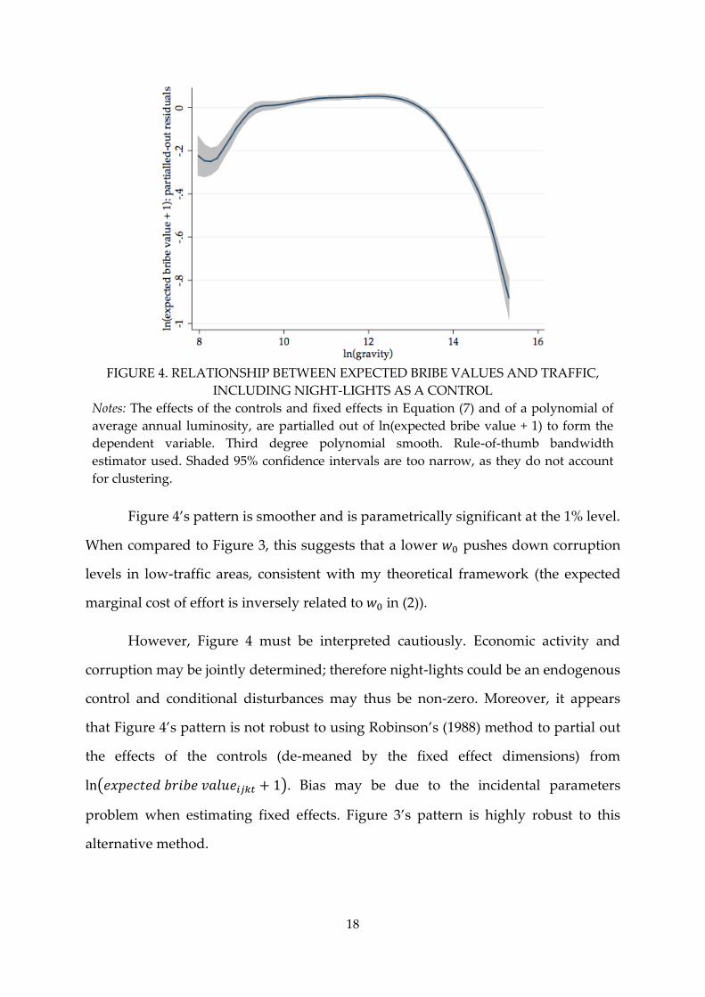
FIGURE 4. RELATIONSHIP BETWEEN EXPECTED BRIBE VALUES AND TRAFFIC,
INCLUDING NIGHT-LIGHTS AS A CONTROL
Notes: The effects of the controls and fixed effects in Equation (7) and of a polynomial of
average annual luminosity, are partialled out of ln(expected bribe value + 1) to form the
dependent variable. Third degree polynomial smooth. Rule-of-thumb bandwidth
estimator used. Shaded 95% confidence intervals are too narrow, as they do not account
for clustering.
Figure 4’s pattern is smoother and is parametrically significant at the 1% level.
When compared to Figure 3, this suggests that a lower 𝑤0 pushes down corruption
levels in low-traffic areas, consistent with my theoretical framework (the expected
marginal cost of effort is inversely related to 𝑤0 in (2)).
However, Figure 4 must be interpreted cautiously. Economic activity and
corruption may be jointly determined; therefore night-lights could be an endogenous
control and conditional disturbances may thus be non-zero. Moreover, it appears
that Figure 4’s pattern is not robust to using Robinson’s (1988) method to partial out
the effects of the controls (de-meaned by the fixed effect dimensions) from
ln(𝑒𝑥𝑝𝑒𝑐𝑡𝑒𝑑𝑏𝑟𝑖𝑏𝑒 𝑣𝑎𝑙𝑢𝑒𝑖𝑗𝑘𝑡 + 1). Bias may be due to the incidental parameters
problem when estimating fixed effects. Figure 3’s pattern is highly robust to this
alternative method.

19
Discussion
Figure 3, my preferred specification, broadly supports the theoretical
predictions of an inverted-U relationship between traffic and corruption. Controlling
for the frequency effect and other sources of heterogeneity, bribery is moderate in
low-traffic areas. As traffic begins to increase, bribery generally increases due to the
benefits of a greater pool of vehicles from which to discriminate. This continues until
a turning point, after which bribery rapidly decreases to low levels in high-traffic
areas. Here, the opportunity cost of marginal extortion is high, and so officials
quickly charge smaller bribes from each vehicle in order to extort from as many as
possible. They trade off price and volume, as suggested by Mookherjee and Png
(1995) and Schleifer and Vishny (1993) in other contexts. Monitoring is also greater in
high-traffic areas.
From a policymaker’s perspective, these results may indicate that anti-
corruption efforts should be targeted towards medium-traffic areas (medium-sized
cities) on the road network, where corruption is highest but where effective
monitoring may be more easily implemented than in more rural areas. There
remains, however, much variation left unexplained by this static analysis (Table 2),
leading me to explore the dynamics of corruption’s spatial distribution.

20
b) How might regional favouritism affect bribe values in the
president’s region of birth?
Context
I explore regional favouritism in Mali. In March 2012, a military coup ended
the 10-year presidency of a former military general (before entering civilian politics).
The coup was condemned. As part of an internationally brokered agreement, the
speaker of parliament was made interim president in April 2012 until elections could
be held in August 2013.
Difference-in-differences
I explore changes in corruption at the checkpoint in Kati, the birth town of the
interim president, once he comes into power; I compare it to a control group of five
other Malian checkpoints, estimating a difference-in-differences (DD) regression for
driver 𝑖 at checkpoint 𝑗 with official 𝑘 on date 𝑡:
(8) ln(𝑏𝑟𝑖𝑏𝑒 𝑣𝑎𝑙𝑢𝑒𝑖𝑗𝑘𝑡 + 1) =𝛽0 + 𝛽1𝐾𝑎𝑡𝑖𝑗 + 𝛽2𝐼𝑛 𝑝𝑜𝑤𝑒𝑟𝑡 + 𝛽3(𝐾𝑎𝑡𝑖𝑗 × 𝐼𝑛 𝑝𝑜𝑤𝑒𝑟𝑡)
+𝛼𝑖 + 𝛼𝑘𝑡 + 𝛿′𝑡𝑟𝑢𝑐𝑘𝑖 + 휀𝑖𝑗𝑘𝑡.
I use actual bribe values for ease of interpretation since all checkpoints analysed are
formal and frequently occupied by officials9. 𝐾𝑎𝑡𝑖𝑗 is a dummy for the interim
president’s region; 𝐼𝑛 𝑝𝑜𝑤𝑒𝑟𝑡 is a dummy for the interim presidency; 𝛼𝑖 are driver
fixed effects to control for driver-specific heterogeneity; 𝛼𝑘𝑡 are official-month-year
fixed effects to dynamically control for heterogeneity between official groups; 𝑡𝑟𝑢𝑐𝑘𝑖
is a vector of truck characteristic dummies. 𝛽3 is the difference-in-differences
estimate. I use data from 1 April 2010 to 30 September 2012 (when my sample ends).
9 Conclusions are the same for expected bribe values.

21
Difference-in-difference-in-differences
Moving to a civilian president after 10 years of a former military president
may affect the behaviour of military officials. They may opportunistically increase
extortion (Cooper, 2015), as the new civilian leader may lack control over them
compared to the previous military leader. Alternatively, with the president no longer
‘one of their own’, they may lose privileges and protection from punishment. This
may also interact with regional favouritism, particularly if there is a response to the
direct involvement of Kati military in the preceding coup.
I therefore investigate potential heterogeneity in favouritism between military
and non-military officials in Kati, estimating a triple differences (DDD) regression:
(9) ln(𝑏𝑟𝑖𝑏𝑒 𝑣𝑎𝑙𝑢𝑒𝑖𝑗𝑘𝑡 + 1) =𝛽0 + 𝛽1𝐾𝑎𝑡𝑖𝑗 + 𝛽2𝐼𝑛 𝑝𝑜𝑤𝑒𝑟𝑡 + 𝛽3(𝐾𝑎𝑡𝑖𝑗 × 𝐼𝑛 𝑝𝑜𝑤𝑒𝑟𝑡)
+ 𝛽4𝑀𝑖𝑙𝑖𝑡𝑎𝑟𝑦𝑘 + 𝛽5(𝐾𝑎𝑡𝑖𝑗 ×𝑀𝑖𝑙.𝑘 ) + 𝛽6(𝐼𝑛 𝑝𝑜𝑤𝑒𝑟𝑡 ×𝑀𝑖𝑙.𝑘 )
+𝛽7(𝐾𝑎𝑡𝑖𝑗 × 𝐼𝑛 𝑝𝑜𝑤𝑒𝑟𝑡 ×𝑀𝑖𝑙.𝑘 ) + 𝛼𝑖 + 𝛿′𝑡𝑟𝑢𝑐𝑘𝑖 + 휀𝑖𝑗𝑘𝑡.
𝑀𝑖𝑙𝑖𝑡𝑎𝑟𝑦𝑘 (𝑀𝑖𝑙.𝑘) is a dummy for military officials. I exclude official-month-year
fixed effects because of the 𝑀𝑖𝑙𝑖𝑡𝑎𝑟𝑦𝑘 interaction terms. All other controls and fixed
effects are as in (8). 𝛽3 and (𝛽3 + 𝛽7) are the DD coefficients for non-military and
military respectively.
The triple differences coefficient, 𝛽7, directly tests for heterogeneous
favouritism across Kati’s official groups.
Baseline results
Baseline results (Table 4, Section A) suggest a significant effect of regional
favouritism on bribery. In Column 1, bribe values increase by approximately 25% in
the president’s region relative to the control. However, this masks significant
heterogeneity at the 1% level (Column 2). Whilst non-military bribe values in Kati

22
rise by approximately 32% relative to control non-military, for military they fall by
approximately 29% (32% - 61%) relative to control military10.
TABLE 4 – DD AND DDD ESTIMATES OF REGIONAL FAVOURITISM
Dependent variable ln(bribe value +1)
A. Baseline
B. Differential time trends
(1) (2) (3) (4)
Kati 0.476*** 0.481***
0.358*** 0.424***
(0.039) (0.043) (0.056) (0.072)
In Power 1.027** 0.422**
1.285** 0.432
(0.450) (0.213) (0.530) (0.293)
Kati x In Power 0.253*** 0.315***
0.119 0.246*
(0.074) (0.096) (0.118) (0.142)
Military
-0.439*** -0.144
(0.073) (0.111)
Kati x Miltary
-0.007 -0.145
(0.085) (0.137)
In Power x Military
0.415** 0.755***
(0.182) (0.271)
Kati x In Power x Military
-0.610*** -0.765***
(0.147) (0.292)
Driver FE Yes Yes
Yes Yes
Truck characteristics Yes Yes
Yes Yes
Official-Month-Year FE Yes No
Yes No
Differential time trends No No
Yes Yes
R-squared 0.366 0.306
0.367 0.310
Observations 10,618 10,618
10,618 10,618
Notes: Differential time trends for the treatment and control are official-specific in (4).
Truck characteristics include truck type, foreign truck and inland journey dummies.
Standard errors, clustered by checkpoint-month and trip, are reported in parentheses;
*** p≤0.01, ** p≤0.05, * p≤0.10.
10 DD coefficients for non-military and military are significant at the 1% and 5% levels.

23
Validity of the difference-in-differences estimator
The key identifying assumption of difference-in-differences is common trends
between the treatment and control groups in the absence of treatment. This is
necessary for the control group to provide a valid counterfactual. Although this is
fundamentally untestable, one can use past observations to test its plausibility.
I divide the sample into 5 six-month periods (there are six months of data
with the interim president in power). Then, for the four periods before his
presidency (April 2010 – March 2012), I estimate the following regression:
(10) ln(𝑏𝑟𝑖𝑏𝑒 𝑣𝑎𝑙𝑢𝑒𝑖𝑗𝑘𝑡 + 1) =𝛽0 + 𝛽1𝐾𝑎𝑡𝑖𝑗 +∑𝛾𝑝𝑃𝑒𝑟𝑖𝑜𝑑𝑝𝑡
𝑝=4
𝑝=2
+∑𝜆𝑞(𝐾𝑎𝑡𝑖𝑗 × 𝑃𝑒𝑟𝑖𝑜𝑑𝑞𝑡)
𝑞=4
𝑞=2
+𝛼𝑖 + 𝛼𝑘𝑡 + 𝛿′𝑡𝑟𝑢𝑐𝑘𝑖 + 휀𝑖𝑗𝑘𝑡.
The ∑ 𝜆𝑞(𝐾𝑎𝑡𝑖𝑗 × 𝑃𝑒𝑟𝑖𝑜𝑑𝑞𝑡)𝑞=4𝑞=2 dummies allow for differential behaviour in Kati,
controlling for first-period differences with the control group. All fixed effects and
controls are as in the baseline DD specification, (8).
TABLE 5 – PARALLEL TRENDS TEST: DIFFERENTIAL BRIBE VALUES IN KATI
BEFORE THE COUP
Oct. 2010 –
Mar. 2011
Apr. 2011 –
Sept. 2011
Oct. 2011 –
Mar. 2012
Differential bribe
values in Kati
0.015 0.235*** 0.037
(0.053) (0.066) (0.085)
Notes: Dependent variable is ln(bribe value + 1); R2=0.368; N=9,592. Full
specification in Equation (10). Standard errors, clustered by checkpoint-month and
trip, are reported in parentheses; *** p≤0.01, ** p≤0.05, * p≤0.10.
Table 5 outlines the results. Bribe prices in Kati are approximately 24% higher
during April – September 2011, controlling for initial differences. This appears to be
a temporary shock without persistence, since there are no differences (beyond initial
differences) in the other six-month periods11. The presence of the one-period shock,
11 The same pattern also holds for both military and non-military individually.

24
however, calls into question whether the control group is a valid counterfactual to
Kati.
The obvious alternative explanation for my baseline results is that another
similar shock occurs in Kati after the coup, rather than regional ‘favouritism’. It is
impossible to rule this out with certainty, since the potential outcome in Kati without
a Kati-born interim president is unobserved. This is always an issue with difference-
in-differences, as even common past trends are never guaranteed to continue into
the future (in the absence of treatment).
I argue, however, that there is still evidence of regional ‘favouritism’. One
way to deal with uncommon trends is to allow the treatment and control groups to
follow different linear time trends (Table 4, Section B). Whilst this reveals an
insignificant difference-in-differences estimate (Column 3), the triple differences
results (Column 4) are consistent with the baseline: a significant increase for non-
military (at the 10% level) and a significantly heterogeneous outcome for military (at
the 1% level)12. However, using a linear trend here is imperfect, since divergence
between Kati and the control does not follow a linear trend; it only occurs in one
period. Therefore, this alone provides only limited additional support for regional
‘favouritism’.
A more convincing argument comes from evaluating the nature of the pre-
coup shock itself; specifically, the extent to which there is heterogeneity within Kati.
To test this, I estimate a ‘placebo’ DDD regression: this replaces the “In Power”
dummy in the baseline DDD, (9), with an “April – September 2011” (pre-coup shock)
dummy, and ends the sample on 30 September 2011. I also estimate baseline and
‘placebo’ DD coefficients for both non-military and military.
12 The -0.519 military DD coefficient is significant at the 5% level.

25
TABLE 6 – HETEROGENEITY WITHIN KATI DURING THE INTERIM PRESIDENCY
AND DURING THE PRE-COUP SHOCK
A. Baseline: Interim Presidency B. ‘Placebo’: April – September 2011
Military Non-military Military Non-military
DD Coeff. -0.295** 0.315***
0.380** 0.070
(0.119) (0.096) (0.185) (0.109)
Difference:
DDD Coeff.
-0.610*** 0.310
(0.147) (0.235)
Notes: Dependent variable is ln(bribe value + 1). Controls and fixed effects in Equation (9).
Standard errors, clustered by checkpoint-month and trip, are reported in parentheses;
*** p≤0.01, ** p≤0.05, * p≤0.10.
Table 6 compares baseline estimates for the interim presidency to placebo
estimates for the shock. During the pre-coup shock (Section B), both DD coefficients
are positive, albeit to varying degrees. DDD estimates reveal no significant
heterogeneity between the two official groups. This indicates a common, rather than
idiosyncratic, shock; such is expected for a typical checkpoint-specific shock. By
contrast, during the interim presidency (Section A), the difference between military
and non-military officials is significant at the 0.1% level. Moreover, there is an
unusually wide divergence in outcomes; the DD coefficients are of equal magnitude
but in opposite directions.
The stark divergence and heterogeneity strongly suggest that bribe patterns in
Kati during the interim presidency are fundamentally different in nature to patterns
during the more typical pre-coup shock. This further strengthens the evidence
supporting my baseline conclusion of heterogeneous regional ‘favouritism’ with a
Kati-born president in power.
Discussion
These results show how regional ‘favouritism’ can affect corruption’s spatial
distribution. Both lower monitoring and better outside options can explain the
increase in bribe values for non-military in Kati; the lack of sub-annual night-lights
data prevents me from assessing the relative importance of these channels. Greater
monitoring of and control over officials in the president’s region (Kasara, 2007)

26
likely explains the reduction for military in Kati, particularly since bribe values rise
sharply for military at control checkpoints during the interim presidency (Table 4,
Column 2). Monitoring may increase as punishment for the Kati military’s direct
involvement in the preceding coup. The divergence highlights that regional
favouritism can have both winners and losers within the president’s region.
Whilst Section IV provides illustrations of how favouritism might work, I
have no evidence of the specific mechanism in this particular context. Therefore,
there is no evidence to directly implicate the president or any other individuals. To
draw direct conclusions, a much greater understanding is required of the political
context and of the operations of the system of Malian officials. My results merely
highlight that regional favouritism may help to explain some patterns in local
corruption, as it can for public good allocation (see Section II).
Favouritism is also heterogeneous across countries and outcomes (Kramon
and Posner, 2013). Therefore I cannot make general conclusions on regional
favouritism’s impact on corruption. External validity is also limited by the preceding
coup, and noise is added by the Kati military’s direct involvement in it. A further
limitation is that my dataset ends within 6 months of the interim presidency. There
exists an extension continuing until September 2013, the month after the subsequent
presidential elections. Although I would be unable to investigate what happens after
the Kati-born president leaves power, the extension would help verify whether my
findings persist throughout the interim presidency. This could help rule out
alternative explanations for my results, and hence show that the significant patterns
only occur because Kati is the president’s region. Unfortunately, I have been unable
to access the extension.
Abadie and Gardeazabal (2003) develop a method to create a valid
counterfactual where trends are uncommon. Their synthetic control group is a
weighted combination of all potential control units; weights are determined by how
well each control unit matches with the treatment unit, during the pre-treatment

27
period. I create a synthetic control group, although its pre-coup bribe patterns do not
match closely enough with Kati’s to draw robust conclusions. Nevertheless, findings
are qualitatively similar to those discussed.
VI. EVALUATION OF MODEL
The rational expected utility framework underlying my theoretical model
usefully isolates certain determinants of corruption. Nevertheless, here I provide a
brief example of its potential shortcomings.
Some aspects of petty corruption are arguably idiosyncratic and behavioural
(Foltz and Opoku-Agyemang, 2015). I highlight this through the relationship
between corruption and rainfall. Weather has been credibly shown to
psychologically affect decision-making in certain economic contexts (Busse et al.,
2015; DellaVigna, 2009; Hirshleifer and Shumway, 2003). I use high-resolution daily
precipitation data to measure rainfall at checkpoint 𝑗 on date 𝑡, estimating:
(11) ln(𝑏𝑟𝑖𝑏𝑒 𝑣𝑎𝑙𝑢𝑒𝑖𝑗𝑘𝑡 + 1) = 𝛽0 +∑𝛽𝑝𝑅𝑎𝑖𝑛𝑓𝑎𝑙𝑙𝑖𝑛𝑡𝑒𝑛𝑠𝑖𝑡𝑦𝑝𝑗𝑡
4
𝑝=1
+ 𝛼𝑖 + 𝛼𝑗𝑘𝑡 + 휀𝑖𝑗𝑘𝑡.
∑ 𝛽𝑝𝑅𝑎𝑖𝑛𝑓𝑎𝑙𝑙𝑖𝑛𝑡𝑒𝑛𝑠𝑖𝑡𝑦𝑝𝑗𝑡4𝑝=1 is a set of dummies for total rainfall on date 𝑡, at 24mm
intervals; 𝛼𝑖 are trip-specific fixed effects to control for driver/truck-specific
heterogeneity; 𝛼𝑗𝑘𝑡 are checkpoint-official-month-year fixed effects to dynamically
control for seasonal fluctuations, and checkpoint and official heterogeneity.
TABLE 7 - ESTIMATED COEFFICIENTS ON RAINFALL DUMMIES
Dependent variable: ln(bribe value + 1)
24 ≤ r < 48 48 ≤ r < 72 72 ≤ r < 96 96 ≤ r
0.000 -0.193 1.662*** -0.689***
(0.045) (0.121) (0.607) (0.123)
Notes: R2=0.555; N=253,559. r=rainfall (in mm). Full specification in Equation
(11). Standard errors, clustered by checkpoint and trip, are reported in
parentheses; *** p≤0.01, ** p≤0.05, * p≤0.10.

28
Relative to 0-24mm rainfall days13, bribes are 427% higher (𝑒1.662 − 1) on 72-
96mm days and 50% lower (𝑒−0.689 − 1) on 96+mm days (Table 7)14. The magnitude
of these significant coefficients dwarfs many results in this paper15.
My intention is not to propose a grand theory of weather and corruption, or
to suggest that this finding cannot be reconciled through certain channels within or
extensions to my traditional model16. 72+mm rainfall days are also too rare to draw
robust conclusions. Nevertheless, given both the unexpected magnitude of these
coefficients and weather’s psychological effect on decision-making in other contexts
(cited above), I merely wish to suggest that behavioural factors could perhaps
explain certain idiosyncrasies of petty corruption. This should not be ignored in the
future research agenda.
VII. CONCLUSION
In this paper, I explore the spatial determinants of corruption on West African
roads. Petty corruption has a broadly inverted-U relationship with traffic: moderate
in low-traffic areas, high in medium-traffic areas, and low in high-traffic areas. I also
find some evidence of heterogeneous regional ‘favouritism’ in Mali; there are both
winners and losers within the president’s region. Finally, I argue for more research
combining corruption and behavioural economics, after finding an unusually large
relationship between bribe values and rainfall.
Although my findings provide some insight into the determinants of
corruption, much remains to be explored. My partial equilibrium analysis does not
consider substitution into other forms of corruption (Olken, 2007) or how corruption
moves up the chain of officials (Basu, Bhattacharya, and Mishra, 1992). It would also
be interesting to estimate spillovers between nearby checkpoints, using spatial
13 Rain showers 10-50mm/hr are ‘heavy’ (UK Met Office). 14 Coefficients are too large to use approximations. 15 My other findings are robust to including rainfall dummies, since heavy rainfall is infrequent. 16 Rainfall may affect traffic and monitoring, for example.

29
econometric techniques, as a test of self-reinforcing corruption models (see Aidt,
2003). This unique dataset provides a special opportunity to explore numerous
questions on corruption in West Africa; I look forward to finding more answers.

30
REFERENCES
Abadie, A., 2005. Semiparametric Difference-in-Differences Estimators. Review of
Economic Studies 72, 1–19.
Abadie, A., Diamond, A., Hainmueller, J., 2010. Synthetic Control Methods for
Comparative Case Studies: Estimating the Effect of California’s Tobacco
Control Program. Journal of the American Statistical Association 105, 493–505.
Abadie, A., Gardeazabal, J., 2003. The Economic Costs of Conflict: A Case Study of
the Basque Country. American Economic Review 93, 113–132.
Aidt, T.S., 2003. Economic analysis of corruption: a survey. The Economic Journal
113, 632–652.
Angrist, J.D., Pischke Jo ̈rn-Steffen, 2009. Mostly harmless econometrics: an
empiricist's companion. Princeton University Press, Princeton.
Banerjee, A., Mullainathan, S., Hanna, R., 2012. Corruption. Unpublished Working
Paper, National Bureau of Economic Research.
Bardhan, P., Mookherjee, D., 2000. Capture and Governance at Local and National
Levels. American Economic Review 90, 135–139.
Basu, K., Bhattacharya, S., Mishra, A., 1992. Notes on bribery and the control of
corruption. Journal of Public Economics 48, 349–359.
Bates, R.H., 1983. Modernization, Ethnic Competition, and the Rationality of Politics
in Contemporary Africa, in: Rothchild, D., Olorunsola, V.A. (Eds.), State
versus Ethnic Claims: African Policy Dilemmas, Westview Press, pp. 152-171.
Becker, G.S., Stigler, G.J., 1974. Law Enforcement, Malfeasance, and Compensation of
Enforcers. The Journal of Legal Studies 3, 1–18.
Bernheim, B.D., Ray, D., Yeltekin, Ş., 2015. Poverty and Self-Control. Econometrica
83, 1877–1911.
Bertrand, M., Duflo, E., Mullainathan, S., 2004. How Much Should We Trust
Differences-In-Differences Estimates? The Quarterly Journal of Economics
119, 249–275.
Bromley, D., Foltz, J., 2011. Sustainability under siege: Transport Costs and
Corruption on West Africa's Trade Corridors. Natural Resources Forum 35,
32–48.
Burgess, R., Hansen, M., Olken, B.A., Potapov, P., Sieber, S., 2012. The Political
Economy of Deforestation in the Tropics. The Quarterly Journal of Economics
127, 1707–1754.

31
Burgess, R., Jedwab, R., Miguel, E., Morjaria, A., Padró i Miquel, G., 2015. The Value
of Democracy: Evidence from Road Building in Kenya. American Economic
Review 105, 1817–1851.
Busse, M.R., Pope, D.G., Pope, J.C., Silva-Risso, J., 2015. The Psychological Effect of
Weather on Car Purchases. The Quarterly Journal of Economics 130, 371–414.
Cameron, A.C., Gelbach, J.B., Miller, D.L., 2011. Robust Inference With Multiway
Clustering. Journal of Business & Economic Statistics 29, 238–249.
Cooper, J.J., 2015. Do Officials Extort More During Elections? Evidence from Micro-
Data on Corruption in Five West African States. Unpublished Working Paper,
SSRN Electronic Journal.
Dellavigna, S., 2009. Psychology and Economics: Evidence from the Field. Journal of
Economic Literature 47, 315–372.
Fan, J. 1992. “Design-Adaptive Nonparametric Regression.” Journal of the American
Statistical Association 87 420, 998–1004.
Foltz, J., Bromley, D., 2010. Highway Robbery: The Economics of Petty Corruption in
West African Trucking. Unpublished working paper, University of
Wisconsin-Madison.
Foltz, J., Opoku-Agyemang, K., 2015. Do Higher Salaries Lower Petty Corruption? A
Policy Experiment on West Africa’s Highways. Unpublished working paper,
University of Wisconsin-Madison and University of California, Berkeley.
Franck, R., Rainer, I., 2012. Does the Leader's Ethnicity Matter? Ethnic Favoritism,
Education, and Health in Sub-Saharan Africa. American Political Science
Review 106, 294–325.
Freund, C., Rocha, N., 2011. What Constrains Africa's Exports? The World Bank
Economic Review 25, 361–386.
Fujita, M., Krugman, P.R., Venables, A., 1999. The spatial economy: cities, regions
and international trade. MIT Press, Cambridge, MA.
Handy, S.L., Niemeier, D.A., 1997. Measuring accessibility: an exploration of issues
and alternatives. Environment and Planning A 29, 1175–1194.
Henderson, J.V., Storeygard, A., Weil, D.N., 2012. Measuring Economic Growth from
Outer Space. American Economic Review 102, 994–1028.
Herbst, J.I., 2000. States and power in Africa: comparative lessons in authority and
control. Princeton University Press, Princeton, NJ.
Hirshleifer, D., Shumway, T., 2003. Good Day Sunshine: Stock Returns and the
Weather. The Journal of Finance 58, 1009–1032.

32
Hodler, R., Raschky, P.A., 2014. Regional Favoritism. The Quarterly Journal of
Economics 129, 995–1033.
Jung, W.-S., Wang, F., Stanley, H.E., 2008. Gravity model in the Korean highway.
Europhysics Letters 81, 48005.
Kasara, K., 2007. Tax Me If You Can: Ethnic Geography, Democracy, and the
Taxation of Agriculture in Africa. American Political Science Review 101, 159.
Kramon, E., Posner, D.N., 2013. Who Benefits from Distributive Politics? How the
Outcome One Studies Affects the Answer One Gets. Perspectives on Politics
11, 461–474.
Lambsdorff, J.G., 2006. Causes and Consequences of Corruption: What Do We Know
from a Cross-Section of Countries?, in: Rose-Ackerman, S. (Ed.), International
Handbook on the Economics of Corruption, Edward Elgar, pp. 3-51.
Lambsdorff, J.G., 2012. Behavioral and Experimental Economics as a Guidance to
Anticorruption, in: Serra, D., Wantcheckon, L. (Eds.), New Advances in
Experimental Research on Corruption, Research in Experimental Economics
15, Emerald Publishing Group, pp. 279-300.
Lowe, M., 2014. Night Lights and ArcGIS: A Brief Guide. Unpublished Working
Paper, Massachusetts Institute of Technology.
McMillan, M., 2001. Why Kill the Golden Goose? A Political-Economy Model of
Export Taxation. Review of Economics and Statistics 83, 170–184.
Michalopoulos, S., Papaioannou, E., 2013. National Institutions and Subnational
Development in Africa. The Quarterly Journal of Economics 129, 151–213.
Mookherjee, D., Png, I.P.L., 1995. Corruptible Law Enforcers: How Should They Be
Compensated? The Economic Journal 105, 145.
Neyman, J., Scott, E.L., 1948. Consistent Estimates Based on Partially Consistent
Observations. Econometrica 16, 1.
Olken, B.A., 2007. Monitoring Corruption: Evidence from a Field Experiment in
Indonesia. Journal of Political Economy 115, 200–249.
Olken, B.A., Barron, P., 2009. The Simple Economics of Extortion: Evidence from
Trucking in Aceh. Journal of Political Economy 117, 417–452.
Olken, B.A., Pande, R., 2012. Corruption in Developing Countries. Annual Review of
Economics 4, 479–509.
Padró i Miquel, G., 2007. The Control of Politicians in Divided Societies: The Politics
of Fear. Review of Economic Studies 74, 1259–1274.

33
Robinson, P.M., 1988. Root-N-Consistent Semiparametric Regression. Econometrica
56, 931–954.
Sequeira, S., Djankov, S., 2014. Corruption and firm behavior: Evidence from African
ports. Journal of International Economics 94, 277–294.
Sevtsuk, A., Mekonnen, M., Kalvo, R., 2016. Urban Network Analysis: Help.
Unpublished Guide, City Form Lab.
Shleifer, A., Vishny, R.W., 1993. Corruption. The Quarterly Journal of Economics
108, 599–617.
Shleifer, A., Vishny, R.W., 1998. The grabbing hand: government pathologies and
their cures. Harvard University Press, Cambridge, MA.
Svensson, J., 2005. Eight Questions about Corruption. Journal of Economic
Perspectives 19, 19–42.
Treisman, D., 2000. The causes of corruption: a cross-national study. Journal of
Public Economics 76, 399–457.
Wooldridge, J.M., 2002. Econometric analysis of cross section and panel data. MIT
Press, Cambridge, MA.