baltimore nonattainment area pm state … · 1.3 sip process ... appendix f – contingency...

MARYLAND DEPARTMENT OF THE ENVIRONMENT 1800 Washington Boulevard • Baltimore MD 21230 410-537-3000 • 1-800-633-6101

Martin O'Malley Governor Anthony Brown Lt. Governor

Shari T. Wilson Secretary Robert M. Summers, Ph.D. Deputy Secretary

Baltimore Nonattainment Area

PM2.5 State Implementation Plan and

Base Year Inventory

SIP Number: 08-04

March 24, 2008

Prepared for:

U.S. Environmental Protection Agency

Prepared by:

Maryland Department of the Environment

This Page Left Intentionally Blank

BNAA PM2.5 SIP 3/24/2008 ii

TABLE OF CONTENTS 1.0 EXECUTIVE SUMMARY ................................................................................................... 1

1.1 INTRODUCTION AND BACKGROUND ........................................................................................ 1 1.2 SIP REQUIREMENTS FOR NONATTAINMENT AREAS ................................................................ 4 1.3 SIP PROCESS........................................................................................................................... 5 1.4 STATE COMMITMENT/IMPLEMENTATION ASSURANCES .......................................................... 5 1.5 SUBMITTAL OF THE PLANS...................................................................................................... 5 1.6 SANCTIONS ............................................................................................................................. 6 1.7 BASE YEAR 2002 EMISSION INVENTORY AND FUTURE YEAR 2009 EMISSION INVENTORY .... 6 1.8 REDUCTIONS IN PM2.5 PRECURSORS FROM MEASURES, 2002-2009........................................ 8 1.9 ESTABLISHMENT OF A BUDGET FOR TRANSPORTATION MOBILE EMISSIONS........................... 8 1.10 ATTAINMENT DEMONSTRATION ............................................................................................. 8 1.11 DETERMINATION OF REASONABLY AVAILABLE CONTROL MEASURES (RACM).................... 9 1.12 CONTINGENCY MEASURES...................................................................................................... 9 1.13 DOCUMENT CONTENTS ........................................................................................................... 9

2.0 FINE PARTICLE POLLUTION ......................................................................................... 11

2.1 DEFINITION OF FINE PARTICLE MATTER............................................................................... 11 2.2 HEALTH AND ENVIRONMENTAL EFFECTS ............................................................................. 11 2.3 SEASONAL VARIATION OF PM2.5 CONSTITUENTS ................................................................ 13 2.4 DIURNAL VARIATION OF FINE PARTICLES ............................................................................ 19 2.5 TRAJECTORIES OF FINE PARTICLES ....................................................................................... 20 2.6 MAJOR CONSTITUENTS OF PM2.5 AND SOURCES IN THE BALTIMORE REGION ..................... 22 2.7 SOURCES OF FINE PARTICLES AND CONSTITUENTS ............................................................... 23 2.8 DETERMINATION OF SIGNIFICANCE FOR PRECURSORS .......................................................... 24

3.0 THE 2002 BASE-YEAR INVENTORY............................................................................. 27

3.1 BACKGROUND AND REQUIREMENTS...................................................................................... 27 3.2 TOTAL EMISSIONS BY SOURCE.............................................................................................. 28

3.2.1 Point Sources .............................................................................................................. 28 3.2.2 Quasi-Point Sources ................................................................................................... 28 3.2.3 Area Sources ............................................................................................................... 28 3.2.4 Mobile Sources............................................................................................................ 29 3.2.5 Nonroad Sources......................................................................................................... 31 3.2.6 Biogenic Emissions ..................................................................................................... 32

4.0 THE 2009 PROJECTED UNCONTROLLED AND CONTROLLED INVENTORIES ... 33

4.1 GROWTH PROJECTION METHODOLOGY................................................................................. 33 4.1.1 Growth Projection Methodology for Point Sources: EGAS ....................................... 33 4.1.2 Growth Projection Methodology for Quasi-Point Sources ........................................ 34 4.1.3 Growth Projection Methodology: Area Sources......................................................... 34 4.1.4 Growth Projection Methodology: Nonroad Model Sources....................................... 36 4.1.5 Growth Projection Methodology: Nonroad Sources .................................................. 38 4.1.6 Growth Projection Methodology: Onroad Sources.................................................... 38 4.1.7 Biogenic Emission Projections ................................................................................... 38

4.2 OFFSET PROVISIONS, EMISSION REDUCTION CREDITS AND POINT SOURCE GROWTH........... 39 4.3 ACTUAL VS. ALLOWABLE EMISSIONS IN DEVELOPMENT OF THE 2009 PROJECTED EMISSIONS

INVENTORIES ........................................................................................................................ 41

4.4 2009 CONTROLLED EMISSIONS FOR ATTAINMENT................................................................ 41 4.4.1 2009 Projected Controlled Inventory: Point Sources................................................. 42 4.4.2 2009 Projected Controlled Inventory: Quasi-Point Sources...................................... 42 4.4.3 2009 Projected Controlled Inventory: Area Sources.................................................. 42 4.4.4 2009 Projected Controlled Inventory: Nonroad Sources ........................................... 42 4.4.5 2009 Projected Controlled Inventory: Onroad Sources............................................. 43

4.5 2009 PROJECTED CONTROLLED INVENTORY – SUMMARY OF EMISSIONS ............................. 44

5.0 CONTROL MEASURES .................................................................................................... 45

5.1 CONTROL MEASURES INCLUDED IN 2002 BASELINE SCENARIO ........................................... 45 5.1.1 Point Source Measures ............................................................................................... 45 5.1.2 Area Source Measures ................................................................................................ 47 5.1.3 On-Road Mobile Measures ......................................................................................... 50 5.1.4 Non-Road Measures.................................................................................................... 51

5.2 CONTROL MEASURES FOR PM2.5 ATTAINMENT..................................................................... 53 5.2.1 Point Sources .............................................................................................................. 53 5.2.2 On-Road Mobile.......................................................................................................... 55 5.2.3 New Non-Road Measures ........................................................................................... 60

5.3 VOLUNTARY AND INNOVATIVE CONTROL MEASURES .......................................................... 65 5.3.1 Regional Forest Canopy Program: Conservation, Restoration, and Expansion ...... 66 5.3.2 Clean Air Teleworking Initiative ................................................................................ 68 5.3.3 High Electricity Demand Day (HEDD) Initiative ...................................................... 72 5.3.4 Emission Reductions from Transportation Measures................................................. 72

6.0 REASONABLY AVAILABLE CONTROL MEASURE (RACM) ANALYSIS .............. 79

6.1 ANALYSIS OVERVIEW AND CRITERIA ................................................................................... 79 6.1.1 Implementation Date................................................................................................... 80 6.1.2 Enforceability.............................................................................................................. 80 6.1.3 Technological Feasibility............................................................................................ 81 6.1.4 Economic Feasibility and Cost Effectiveness ............................................................. 81 6.1.5 Substantial and Widespread Adverse Impacts............................................................ 81 6.1.6 De Minimis Threshold................................................................................................. 81 6.1.7 Advancing Achievement of Annual 15.0 mg/ m3 Standard......................................... 81 6.1.8 Intensive and Costly Effort.......................................................................................... 82

6.2 RACM MEASURE ANALYSIS................................................................................................ 82 6.2.1 Analysis Methodology................................................................................................. 82 6.2.2 Analysis Results .......................................................................................................... 82

6.3 RACM DETERMINATION...................................................................................................... 82 6.4 RACT APPLICABILITY.......................................................................................................... 82

7.0 MOBILE SOURCE CONFORMITY.................................................................................. 85

7.1 SIGNIFICANCE OF PM2.5 POLLUTANTS AND PRECURSORS FOR THE BALTIMORE, MD NONATTAINMENT AREA ....................................................................................................... 85

7.2 TRANSPORTATION CONFORMITY .......................................................................................... 85 7.2.1 Responsibility for Making a Conformity Determination ............................................ 86 7.2.2 Mobile Emissions Budget and the Baltimore Region Transportation Conformity

Process........................................................................................................................ 87 7.3 BUDGET LEVEL FOR ON-ROAD MOBILE SOURCE EMISSIONS................................................ 87

7.3.1 Modeling and Data ..................................................................................................... 87

BNAA PM2.5 SIP 3/24/2008 ii

7.3.2 Attainment Year Mobile Budgets ................................................................................ 87

8.0 1997 PM2.5 NONATTAINMENT AREA PLAN COMMITMENTS ................................. 89

8.1 SCHEDULE OF ADOPTED CONTROL MEASURES..................................................................... 89 8.3 RACT APPLICABILITY.......................................................................................................... 91 8.4 REVISION OF NEW SOURCE REVIEW (NSR) REGULATIONS .................................................. 91

9.0 ATTAINMENT PLAN DEMONSTRATION AND WEIGHT OF EVIDENCE............... 93

9.1 MODELING STUDY OVERVIEW.............................................................................................. 93 9.1.1 Background and Objectives ........................................................................................ 93 9.1.2 Relationship to Regional Modeling Protocols............................................................ 95 9.1.3 Conceptual Model....................................................................................................... 95

9.2 DOMAIN AND DATABASE ISSUES .......................................................................................... 96 9.2.1 Episode Selection........................................................................................................ 96 9.2.2 Size of the Modeling Domain...................................................................................... 96 9.2.3 Horizontal Grid Size ................................................................................................... 96 9.2.4 Vertical Resolution...................................................................................................... 97 9.2.5 Initial and Boundary Conditions ................................................................................ 97 9.2.6 Meteorological Model Selection and Configuration .................................................. 97 9.2.7 Emissions Model Selection and Configuration........................................................... 97 9.2.8 Air Quality Model Selection and Configuration......................................................... 98 9.2.9 Quality Assurance....................................................................................................... 98

9.3 MODEL PERFORMANCE EVALUATION ................................................................................... 99 9.3.1 Overview ..................................................................................................................... 99 9.3.2 Diagnostic and Operational Evaluation..................................................................... 99 9.3.3 Summary of Model Performance .............................................................................. 108

9.4 ATTAINMENT DEMONSTRATION ......................................................................................... 108 9.4.1 Overview ................................................................................................................... 108 9.4.2 Modeled Attainment Test .......................................................................................... 109 9.4.3 Unmonitored Area Analysis...................................................................................... 114 9.4.4 Local Area Analysis .................................................................................................. 115 9.4.5 Emissions Inventories ............................................................................................... 115

9.5 WEIGHT OF EVIDENCE DEMONSTRATION............................................................................ 115 9.5.1 Trend in PM2.5 Design Values................................................................................... 116 9.5.2 The Composition of PM2.5......................................................................................... 118 9.5.3 Review of Literature on PM2.5................................................................................... 118 9.5.4 PM2.5 Trends Over the Mid-Atlantic Region............................................................. 119 9.5.5 PM2.5 Composition As it Relates to Effectiveness of Controls.................................. 119 9.5.6 Monitoring Data From Surface-Based Speciation Sites........................................... 120 9.5.7 CMAQ PM2.5 Modeling............................................................................................. 120

9.6 SUMMARY AND CONCLUSIONS OF ATTAINMENT DEMONSTRATION.................................... 121 9.7 PROCEDURAL REQUIREMENTS ............................................................................................ 121

9.7.1 Reporting................................................................................................................... 121 9.7.2 Data Archival and Transfer of Modeling Files......................................................... 121

10.0 CONTINGENCY PLAN ................................................................................................... 123

10.1 CONTINGENCY MEASURES FOR THE ATTAINMENT DEMONSTRATION ................................. 123 10.1.1 Background............................................................................................................... 123 10.1.2 Required Reductions ................................................................................................. 123

BNAA PM2.5 SIP 3/24/2008 iii

10.1.3 Identified Contingency Measures ............................................................................. 124

APPENDICES Appendix A –Base Year Emission Inventory

Appendix A-1: Base Year Emission Inventory Methodologies Appendix A-2: Point Source Base Year Inventory Appendix A-3: Quasi-Point Source Base Year Inventory Appendix A-4: Area Source Base Year Inventory Appendix A-5: Mobile Source Base Year Inventory Appendix A-6: Nonroad Source Base Year Inventory

Appendix B – Projection Year Methodologies Appendix C – Reasonably Available Control Measures (RACM) Analysis

Appendix C-1: List of Potential RACM Control Measures & Analysis Appendix C-2: BMC Reduction Measures List & Analysis

Appendix D –Mobile Budget Documentation Appendix E – OTC MOU Appendix F – Contingency Synopsis of the ASIP Sensitivity Study Appendix G – Attainment Modeling

Appendix G-1: Conceptual Model Appendix G-2: Modeling Domain Boundary Appendix G-3: Horizontal Grid Definitions for MM5 and CMAQ Modeling Domain Appendix G-4: Vertical Layer Definitions for MM5 and CMAQ Modeling Domain Appendix G-5: MM5 Model Configuration Appendix G-6: MM5 Model Performance Evaluation Appendix G-7: SMOKE Processing Description and Configuration Appendix G-8: CMAQ Configuration Appendix G-9: CMAQ Model Performance Appendix G-10: Additional Information on Design Value Calculations Appendix G-11: Weight of Evidence Report

BNAA PM2.5 SIP 3/24/2008 iv

INDEX OF TABLES TABLE 2-1: EPA SIP REQUIREMENTS FOR PM POLLUTANTS.............................................................. 25

TABLE 2-2: SUMMARY OF SIGNIFICANCE DETERMINATIONS FOR SIP CONTROLS AND MOTOR VEHICLE EMISSION BUDGETS ............................................................................................................................. 26

TABLE 2-3: SUMMARY OF RATIONALE FOR VOC AND NH3 INSIGNIFICANCE DETERMINATIONS FOR SIP CONTROLS .................................................................................................................................... 26

TABLE 3-1: 2002 BASE-YEAR ANNUAL INVENTORY ........................................................................... 27

TABLE 4-1: 2002-2009 AREA SOURCE GROWTH FACTORS ................................................................. 34

TABLE 4-2: 2009 NONROAD MODEL INPUTS ................................................................................... 37

TABLE 4.3: EMISSION REDUCTION CREDITS ........................................................................................ 39

TABLE 4-4: 2009 PROJECTED CONTROLLED ANNUAL INVENTORY (TPY)........................................... 44

TABLE 5-1: MARYLAND HEALTHY AIR ACT ANNUAL NOX EMISSIONS REDUCTIONS (TPY): ........... 54

TABLE 5-2: ON-ROAD MOBILE EMISSIONS REDUCTIONS (TPY): ....................................................... 56

TABLE 5-3: OFF-ROAD MOBILE EMISSIONS REDUCTIONS (TPY): ...................................................... 61

TABLE 5-4: CLEAN AIR TELEWORKING TIME LINE.............................................................................. 71

TABLE 7-1: 2009 ATTAINMENT MOBILE BUDGETS FOR THE BALTIMORE NONATTAINMENT AREA.... 88

TABLE 8-1: MARYLAND SCHEDULE OF ADOPTED CONTROL MEASURES ............................................. 89

TABLE 8-2: STATIONARY SOURCE PERMITTING REVISIONS................................................................. 91

TABLE 9-1: BALTIMORE NAA DESIGNATIONS FOR 24-HOUR AND ANNUAL PM2.5 STANDARDS ......... 93

TABLE 9-2. EPA PM2.5 MODELING PERFORMANCE GOALS .............................................................. 100

TABLE 9-3. VISTAS RPO PM2.5 MODELING PERFORMANCE GOALS............................................... 100

TABLE 9-4 ANNUAL SMAT RESULTS FOR BALTIMORE NAA 2009 BEYOND-ON-THE-WAY CONTROL MEASURES......................................................................................................................................... 112

TABLE 9-5. 24-HOUR MODELING ATTAINMENT TEST USING EPA SMAT METHODOLOGY 2009 BEYOND-ON-THE-WAY CONTROL MEASURES.................................................................................. 113

TABLE 10-1: CONTINGENCY REQUIREMENT FOR PM AND PM PRECURSORS .................................... 123

TABLE 10-2: CONTINGENCY MEASURES FOR 2008 PM2.5 ATTAINMENT........................................... 124

BNAA PM2.5 SIP 3/24/2008 v

INDEX OF FIGURES FIGURE 1-1: BALTIMORE, MD PM2.5 NON-ATTAINMENT AREA .......................................................... 3

FIGURE 1-2: BALTIMORE NON-ATTAINMENT AREA PM2.5 MONITORS................................................... 4

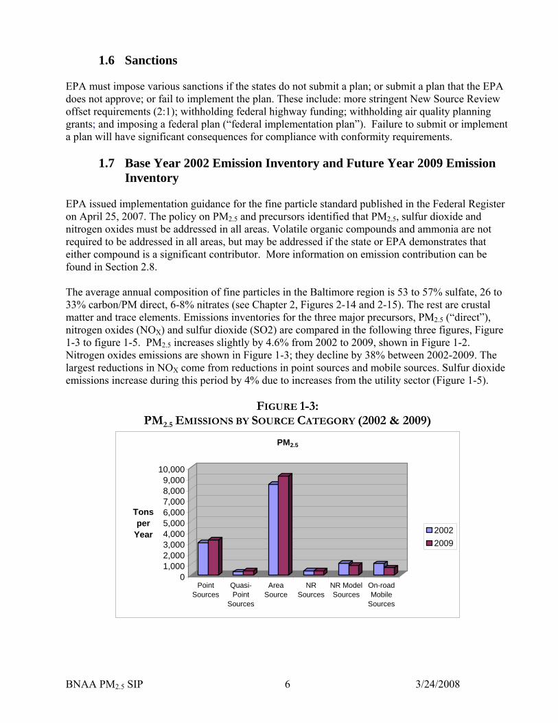
FIGURE 1-3: PM2.5 EMISSIONS BY SOURCE CATEGORY (2002 & 2009) ................................................. 6

FIGURE 1-4: NOX EMISSIONS BY SOURCE CATEGORY (2002 & 2009)................................................... 7

FIGURE 1-5: SO2 EMISSIONS BY SOURCE CATEGORY (2002 & 2009).................................................... 7

FIGURE 2-1: ATMOSPHERIC CHEMICAL REACTIONS THAT CONTRIBUTE TO PM2.5 ............................. 12

FIGURE 2-2: SEASONAL VARIATION OF PM2.5 DURING 2000-2006 IN THE BALTIMORE, MD NON-ATTAINMENT AREA .............................................................................................................................. 13

FIGURE 2-3: SEASONAL VARIATION OF SULFATE PM2.5 (ESSEX MONITOR, 2001-2005) ...................... 14

FIGURE 2-4: SEASONAL VARIATION OF SULFATE PM2.5 (FT. MEADE MONITOR, 2002-2004) ............. 14

FIGURE 2-5: SEASONAL VARIATION OF NITRATE PM2.5 (ESSEX MONITOR, 2001-2005) ...................... 15

FIGURE 2-6: SEASONAL VARIATION OF NITRATE PM2.5 (FT. MEADE MONITOR, 2002-2004) .............. 16

FIGURE 2-7: SEASONAL VARIATION OF ORGANIC CARBON (ESSEX MONITOR, 2001-2005) ................. 17

FIGURE 2-8: SEASONAL VARIATION OF ORGANIC CARBON (FT. MEADE MONITOR, 2002-2004) ......... 17

FIGURE 2-9: SEASONAL VARIATION OF AMMONIUM (ESSEX MONITOR, 2001-2005) ............................ 18

FIGURE 2-10: SEASONAL VARIATION OF AMMONIUM (FT. MEADE MONITOR, 2002-2004) ................. 19

FIGURE 2-11: DIURNAL PM2.5 PATTERN – BALTIMORE NONATTAINMENT AREA ................................ 20

FIGURE 2-12A: PM FINE BACK TRAJECTORIES ...................................................................................... 21

FIGURE 2-12B: PM FINE BACK TRAJECTORIES ...................................................................................... 21

FIGURE 2-13: ANNUALLY AVERAGED 2001-2003 CONCENTRATIONS OF PM2.5 CONSTITUENTS FOR BALTIMORE, MD ................................................................................................................................ 22

FIGURE 2-14: PM2.5 COMPOSITION DATA FROM THE ESSEX, MD MONITOR ...................................... 23

FIGURE 2-15: PM2.5 COMPOSITION DATA FROM THE FT. MEADE, MD MONITOR .............................. 24

FIGURE 5.1 AIR QUALITY ACTION GUIDE............................................................................................ 69

FIGURE 9-1: BALTIMORE NAA AND SURROUNDING REGIONS............................................................. 94

FIGURE 9-2. LOCATIONS USED FOR THE MODEL EVALUATION ACROSS THE OTR+ REGION: FRM (●, 264), STN (■, 50), AND IMPROVE (▲, 21) .................................................................................... 102

FIGURE 9-3. COMPOSITE FRM TIME SERIES ACROSS THE OTR+ REGION (264 MONITORS).............. 103

FIGURE 9-4. MFE AND MFB TIME SERIES FOR FRM PM2.5 ACROSS THE OTR+ REGION ................ 103

FIGURE 9-5. MFE BUGLE PLOT FOR FRM PM2.5 ACROSS OTR+ REGION ......................................... 104

FIGURE 9-6. MFE BUGLE PLOT FOR SO4 ACROSS OTR+ REGION ..................................................... 104

FIGURE 9-7. MFE BUGLE PLOT FOR NO3 ACROSS OTR+ REGION .................................................... 105

FIGURE 9-8. MFE BUGLE PLOT FOR NH4 ACROSS OTR+ REGION..................................................... 105

FIGURE 9-9. MFE BUGLE PLOT FOR EC ACROSS OTR+ REGION....................................................... 106

BNAA PM2.5 SIP 3/24/2008 vi

FIGURE 9-10. MFE BUGLE PLOT FOR OM ACROSS OTR+ REGION ................................................... 106

FIGURE 9-11. MFE BUGLE PLOT FOR SOIL/CRUSTAL ACROSS OTR+ REGION .................................. 107

FIGURE 9-11. BALTIMORE NONATTAINMENT AREA PM2.5 MONITORS USED IN THE MODELING DEMONSTRATION............................................................................................................................... 114

FIGURE 9-12. ANNUAL PM2.5 DESIGN VALUES FOR BALTIMORE NONATTAINMENT AREA FROM 2002-2006. ................................................................................................................................................. 117

FIGURE 9-13. 24-HOUR PM2.5 DESIGN VALUE FOR BALTIMORE NONATTAINMENT AREA FROM 2002-2006. ................................................................................................................................................. 117

BNAA PM2.5 SIP 3/24/2008 vii


BNAA PM2.5 SIP 3/24/2008 viii

1.0 EXECUTIVE SUMMARY

1.1 Introduction and Background Fine particle matter consists of tiny airborne particles that result from particulate emissions, condensation of sulfates, nitrates, and organics from the gas phase, and coagulation of smaller particles. Unlike fine particles, mechanical processes including wind and erosion usually produce coarse-mode particles such as dust, pollen, sea salt, and ash. Fine particles (PM2.5) are less than or equal to 2.5 microns across, about 1/30th the average width of a human hair, while coarse-mode particles are more than 2.5 to around 10 microns across. The size of particles is directly linked to their potential for causing health problems. Fine particles less than 2.5 microns in diameter pose the greatest problems because they can lodge deep into your lungs and some may get into your bloodstream. Therefore, exposure to such particles can affect both lungs and heart. Fine particle pollution affects both human health and the environment such as crops and vegetation. Particle pollution exposure is linked to a variety of health problems, including: Increased respiratory symptoms, such as irritation of the airways, coughing, or difficulty breathing, decreased lung function, aggravated asthma, development of chronic bronchitis, irregular heartbeat, nonfatal heart attacks, and premature death in people with heart or lung disease. The Clean Air Act was passed in 1970 to protect public health and welfare. Congress amended the Act in 1990 to establish requirements for areas not meeting the National Ambient Air Quality Standards (NAAQS). The CAAA established a process for evaluating air quality in each region and identifying nonattainment areas according to the severity of its air pollution problem. The Clean Air Act sets health standards for six ambient pollutants: carbon monoxide, sulfur dioxide, nitrogen oxides, ozone, lead and particulate matter. The Environmental Protection Agency establishes rules and regulations to implement the Clean Air Act. In 1997 EPA reviewed PM air quality criteria and standards and established two new PM2.5 standards: an annual standard of 15.0 µg/m3 and a 24-hour of 65 µg/m3. EPA revised the secondary standards, making them identical to the primary standards. There were a series of legal challenges to the PM standards that were not resolved until March 2002, at which time the standards and EPA’s decision process were upheld. In January 2005 EPA designated the Baltimore area as a nonattainment area for the annual PM2.5 standard. EPA did not use a classification system for PM2.5 nonattainment areas. The boundary of the Baltimore nonattainment area is defined in the Federal Register, Vol.; 70, No. 3, 1/5/05. The Baltimore PM2.5 nonattainment area includes Anne Arundel County, Baltimore County, Baltimore City, Carroll County, Howard County, and Harford County. A map of the nonattainment area is shown in Figure 1-1. States with nonattainment areas must submit to EPA by April 5, 2008, an attainment demonstration and associated air quality modeling, adopted State regulations to reduce emissions of PM2.5 and its precursors, and other supporting information demonstrating that the area will attain the standards as expeditiously as practicable.1 EPA will determine the region’s attainment based on air quality data

1 CAAA Section 172 (a)(2) requires states to attain the standard as expeditiously as possible but within five years of designation.

BNAA PM2.5 SIP 3/24/2008 2

for 2007-2009. The Baltimore nonattainment area is required to attain the standard no later than April 2010. This document, the Baltimore Nonattainment Area PM2.5 State Implementation Plan and Base Year Inventory, is a plan to demonstrate continued improvement and compliance with the annual National Ambient Air Quality Standard (NAAQS) for fine particles in the Baltimore region in 2009. The Plan consists of a Base Year inventory for 2002, a projection inventory for 2009; an attainment plan; a demonstration of reasonably available control measures; mobile budgets for 2009 and 2010, attainment demonstration; and contingency plans for attainment. The plan has been prepared by the Maryland Department of the Environment (MDE) to comply with the Clean Air Act Amendments of 1990 and with EPA requirements for the Baltimore region as stated in EPA’s 2005 designation of the Baltimore region, and EPA’s Clean Air Fine Particle Implementation Rule.2

2 Federal Register, 40 CFR 51, Part II, Clean Air Fine Particle Implementation Rule, Vol.72, No. 79, 4/25/07, pp.20586-20667.

FIGURE 1-1: BALTIMORE, MD PM2.5 NON-ATTAINMENT AREA

BNAA PM2.5 SIP 3 3/24/2008

Baltimore, MDHagerstown-Martinsburg, MD-WV

Washington, DC-MD-VA

Fine Particulate Matter (PM2.5) Non-Attainment Areas in Maryland and Surrounding Jurisdictions

FRM PM-Fine Monitors in Maryland

Baltimore, MDBaltimore, MDHagerstown-Martinsburg, MD-WVHagerstown-Martinsburg, MD-WV

Washington, DC-MD-VAWashington, DC-MD-VA

Fine Particulate Matter (PM2.5) Non-Attainment Areas in Maryland and Surrounding Jurisdictions

FRM PM-Fine Monitors in MarylandFRM PM-Fine Monitors in Maryland

FIGURE 1-2: BALTIMORE NON-ATTAINMENT AREA PM2.5 MONITORS


PM2.5 Monitor


PM2.5 Monitor

Baltimore Nonattainment AreaBaltimore Nonattainment Area

PM2.5 MonitorPM2.5 Monitor

1.2 SIP Requirements for Nonattainment Areas The Clean Air Act Section 172 of subpart 1 describes the general requirements for state implementation plans and Section 110 (a)(2) establishes further requirements.

• Attainment demonstration due 3 years after designation (4/5/08) • RACT/RACM required for major sources • Basic Inspection and Maintenance (I/M) for vehicles • Contingency measures required for failure to attain

EPA issued implementation guidance for the fine particle standard published in the Federal Register on April 25, 2007 (40 CFR 51, Part II, Clean Air Fine Particle Implementation Rule, Vol.72, No. 79, 4/25/07, pp.20586-20667). The policy on PM2.5 and precursors identified that PM2.5, sulfur dioxide and nitrogen oxides must be addressed in all areas. Volatile organic compounds and ammonia are not required to be addressed in all areas, but may be addressed if the state or EPA demonstrates that either compound is a significant contributor. The Annual and 24-Hour Fine Particle Attainment Plan for the Baltimore nonattainment areas has been developed by the Maryland Department of the Environment (MDE). The control measures used to demonstrate compliance with the annual PM2.5 standard in 2009 are presented in Section 5.2.

BNAA PM2.5 SIP 4 3/24/2008

BNAA PM2.5 SIP 3/24/2008 5

1.3 SIP Process

The Act requires states to develop and implement ozone reduction strategies in the form of a SIP. The SIP is the state's "master plan" for attaining and maintaining the NAAQS. Once the administrator of the EPA approves a state plan, the plan is enforceable as a state law and as federal law under Section 113 of the Act. If EPA finds the SIP inadequate to attain the NAAQS in all or any regions of the state, and if the state fails to make the requisite amendments, the EPA administrator may issue binding amendments under Section 110(c)(1). EPA is required to impose severe sanctions on the states under three circumstances: the state's failure to submit a SIP revision; on the finding of the inadequacy of the SIP to meet prescribed air quality requirements; and the state's failure to enforce the control strategies that are contained in the SIP. Sanctions include more stringent New Source Review offset requirements (2:1) and the withholding of federal funds for highway projects -- other than those for safety, mass transit, or transportation improvement projects related to air quality improvement or maintenance -- beginning 24 months after EPA announcement. No federal agency or department will be able to award a transportation grant or fund, license, or permit any other transportation project that does not conform to the most recently approved SIP.

1.4 State Commitment/Implementation Assurances The measures in the SIP must be supported by any necessary legislative authority and adopted by the applicable governmental body responsible for their implementation. Section 110 of the 1990 CAAA specifies the conditions under which EPA approves SIP submissions. These requirements are being followed by Maryland in developing this air quality plan or SIP. In order to develop effective control strategies, EPA has identified four fundamental principles that SIP control strategies must adhere to in order to achieve the desired emissions reductions. These four fundamental principles are outlined in the General Preamble to Title I of the Clean Air Act Amendments of 1990 at Federal Register 13567 (EPA, 1992a). The four fundamental principles are:

a) Emissions reductions ascribed to the control measure must be quantifiable and measurable; b) The control measures must be enforceable, in that the state must show that they have adopted

legal means for ensuring that sources are in compliance with the control measure; c) Measures are replicable; and d) Enforceable.

1.5 Submittal of the Plans

These plans are developed through a public process, formally adopted by the State, and submitted by the Governor's designee to EPA. The Clean Air Act requires EPA to review each plan and any plan revisions and to approve the plan or plan revisions if consistent with the Clean Air Act (the Act).

1.6 Sanctions EPA must impose various sanctions if the states do not submit a plan; or submit a plan that the EPA does not approve; or fail to implement the plan. These include: more stringent New Source Review offset requirements (2:1); withholding federal highway funding; withholding air quality planning grants; and imposing a federal plan (“federal implementation plan”). Failure to submit or implement a plan will have significant consequences for compliance with conformity requirements.

1.7 Base Year 2002 Emission Inventory and Future Year 2009 Emission Inventory

EPA issued implementation guidance for the fine particle standard published in the Federal Register on April 25, 2007. The policy on PM2.5 and precursors identified that PM2.5, sulfur dioxide and nitrogen oxides must be addressed in all areas. Volatile organic compounds and ammonia are not required to be addressed in all areas, but may be addressed if the state or EPA demonstrates that either compound is a significant contributor. More information on emission contribution can be found in Section 2.8. The average annual composition of fine particles in the Baltimore region is 53 to 57% sulfate, 26 to 33% carbon/PM direct, 6-8% nitrates (see Chapter 2, Figures 2-14 and 2-15). The rest are crustal matter and trace elements. Emissions inventories for the three major precursors, PM2.5 (“direct”), nitrogen oxides (NOX) and sulfur dioxide (SO2) are compared in the following three figures, Figure 1-3 to figure 1-5. PM2.5 increases slightly by 4.6% from 2002 to 2009, shown in Figure 1-2. Nitrogen oxides emissions are shown in Figure 1-3; they decline by 38% between 2002-2009. The largest reductions in NOX come from reductions in point sources and mobile sources. Sulfur dioxide emissions increase during this period by 4% due to increases from the utility sector (Figure 1-5).

FIGURE 1-3: PM2.5 EMISSIONS BY SOURCE CATEGORY (2002 & 2009)

01,0002,0003,0004,0005,0006,0007,0008,0009,000

10,000

Tons per

Year

PointSources

Quasi-Point

Sources

AreaSource

NRSources

NR ModelSources

On-roadMobile

Sources

PM2.5

20022009

BNAA PM2.5 SIP 3/24/2008 6

FIGURE 1-4: NOX EMISSIONS BY SOURCE CATEGORY (2002 & 2009)

0

10,000

20,000

30,000

40,000

50,000

60,000

70,000

Tons per

Year

PointSources

Quasi-Point

Sources

AreaSource

NRSources

NR ModelSources

On-roadMobile

Sources

NOX

20022009

FIGURE 1-5: SO2 EMISSIONS BY SOURCE CATEGORY (2002 & 2009)

0

20,000

40,000

60,000

80,000

100,000

120,000

Tons per

Year

PointSources

Quasi-Point

Sources

AreaSource

NRSources

NR ModelSources

On-roadMobile

Sources

SO2

20022009

BNAA PM2.5 SIP 3/24/2008 7

1.8 Reductions in PM2.5 Precursors from Measures, 2002-2009 Overall, the 2009 plan for the Baltimore region includes total reductions by 2009 of 47,818 tons per year of nitrogen oxides (NOX). The plan may be summarized as follows:

• NOX reductions are from State NOX Reasonably Available Control Technologies (RACT) and the Healthy Air Act, EPA Non-road gasoline engines rule, and a suite of on-road measures including High-tech Vehicle Inspection and Maintenance programs, National Low Emission Vehicle Program, Tier 2 Motor Vehicle Emissions Standards.

1.9 Establishment of a Budget for Transportation Mobile Emissions

As part of the development of the plan, MDE in consultation with the Baltimore Regional Transportation Planning Board (BRTB) will establish mobile source emissions budgets or maximum allowable levels of PM2.5 direct and NOX. These budgets will be the benchmark used to determine if the region’s long-range transportation plan, known as “Transportation 2030” and the shorter term Transportation Improvement Program (TIP) conform with the CAAA of 1990. Under EPA regulations the projected mobile source emissions for 2009 -- minus the vehicle technology, fuel, or maintenance-based measures -- become the mobile emissions budgets for the region unless MDE takes actions to set another budget level. The mobile emissions budgets were developed using computer models MOBILE 6.2.03 and HTMS. Attainment Year Mobile Budgets The mobile emissions budgets for the 2009 attainment year are based on the projected 2009 mobile source emissions accounting for all the mobile control measures, and vehicle technology, fuel, or maintenance-based measures. Unlike the Ozone SIP mobile budgets that are based on daily emissions, the PM2.5 mobile budgets are based on annual emissions. The mobile emissions budgets for the 2009 Attainment Year are 686.97 tons/year PM2.5 direct and 36,502.41 tons/year NOX.

The annual Mobile Emissions Budget for 2009 attainment year, based upon the projected 2009 mobile source emissions accounting for all the mobile control measures, and vehicle technology, fuel, or maintenancebased measures: PM2.5 Direct = 686.97 tons/year NOx = 36,502.41 tons/year

-

1.10 Attainment Demonstration

This PM2.5 Attainment Plan includes a modeling demonstration that the Baltimore region will comply with both the 24-Hour and the annual PM2.5 standard in 2009. The demonstration is based on results from the Community Multiscale Air Quality Model (CMAQ). In the base year 2002, monitors in the region were above the annual standard of 15.0 ug/m3. Modeling the projected controlled emissions with reductions from the measures listed in Chapter 5, the results show no monitors in the Baltimore, MD region above the annual PM2.5 health standard of 15.0 ug/m3.

BNAA PM2.5 SIP 3/24/2008 8

BNAA PM2.5 SIP 3/24/2008 9

1.11 Determination of Reasonably Available Control Measures (RACM)

The cumulative impact of previously adopted and on-going measures, described in Chapter 5, will be sufficient to comply with the PM2.5 NAAQS (1997). Maryland will continue to implement the RACM measures already adopted and described in Section 5. The analysis in Chapter 6 establishes that these measures contributed to the region being able to comply with the PM2.5 NAAQS (1997) based on 2003-2005 annual design values. Therefore, this analysis demonstrates that there are no additional measures that are necessary to demonstrate attainment as expeditiously as practicable and to meet any RFP requirements and there are no potential measures that if considered collectively would advance the attainment year by one year or more. The above analysis meets the applicable statutory requirements set forth at Section 172(c)(1) of the Clean Air Act and the applicable regulatory requirements set forth at 40 C.F.R. Section 51.1010.

1.12 Contingency Measures The Healthy Air Act provides a total benefit of more than 80,000 tons per year (tpy) of SO2 in 2010. These SO2 reductions are more than 12 times the required NOX reductions under contingency, and this 12:1 ratio is significantly higher than any of the equivalency assessments described in Section 10. Therefore the Healthy Air Act fulfills the contingency measure requirement.

1.13 Document Contents Chapter 2 presents a detailed overview of fine particle pollution, including a precursor

significance determination Chapter 3 presents revisions to the 2002 base year inventory using MOBILE 6.2.03 and

HTMS including corrections to nonroad, area and stationary source emissions Chapter 4 presents the 2009 projected inventories using MOBILE 6.2.03 and HTMS and

a discussion of the growth projection methodology Chapter 5 Outlines the control strategies that the states will implement to achieve the

reductions in PM2.5, NOX, and SO2, including Supplemental Measures Chapter 6 discusses the demonstration of Reasonably Available Control Measures

(RACM) Chapter 7 discusses mobile source conformity issues and establishes mobile emissions

budgets for the region Chapter 8 presents the schedules and adoption of regulations to meet requirements for

severe nonattainment areas and presents commitments to EPA Chapter 9 presents the Baltimore region’s demonstration of attainment based on CMAQ

modeling Chapter 10 presents contingency measures for the 2009 attainment demonstration.

BNAA PM2.5 SIP 3/24/2008 10


BNAA PM2.5 SIP 3/24/2008 11

2.0 FINE PARTICLE POLLUTION

2.1 Definition of Fine Particle Matter Fine particle matter consists of tiny airborne particles that result from direct particulate emissions, condensation of sulfates, nitrates, and organics from the gas phase, and the coagulation of smaller particles. Unlike fine particles, coarse particles such as dust, pollen, sea salt, and ash, are usually produced by mechanical processes such as wind and erosion. Fine particles (PM2.5) are less than or equal to 2.5 microns across, about 1/30th the average width of a human hair, while coarse-mode particles are more than 2.5 to around 10 microns across. Gas-phase precursors SO2, NOX, VOC, and ammonia undergo chemical reactions in the atmosphere to form secondary particulate matter. Formation of secondary PM depends on numerous factors including the concentrations of precursors, the concentrations of other gaseous reactive species, atmospheric conditions such as solar radiation, temperature, and relative humidity (RH), and the interactions of precursors with preexisting particles and with cloud or fog droplets. Several atmospheric aerosol species, such as ammonium nitrate and certain organic compounds, are semi-volatile and are found in both gas and particle phases. Given the complexity of PM2.5 formation processes, new information from the scientific community continues to emerge to improve our understanding of the relationship between sources of PM precursors and secondary PM formation. Federal Reference Monitors (FRM) sample fine particles in the Baltimore and Washington regions and Washington County Maryland (see Figure 1-1). The purpose of the filter-based FRM monitors is to determine compliance with the PM2.5 NAAQS. FRM monitors are filter-based that measure PM2.5 mass by passing a measured volume of air through a pre-weighed filter.

2.2 Health and Environmental Effects The size of particles is directly linked to their potential for causing health problems. Fine particles less than 2.5 microns in diameter pose the greatest problems because they can lodge deep into the lungs and some may get into the bloodstream. Therefore, exposure to such particles can affect both lungs and heart. Particle pollution exposure is linked to a variety of health problems, including: increased respiratory symptoms, such as irritation of the airways, coughing, or difficulty breathing, decreased lung function, aggravated asthma, development of chronic bronchitis, irregular heartbeat, nonfatal heart attacks, and premature death in people with heart or lung disease. Another concern with fine particles is that there can be adverse impacts from PM2.5 pollution all year versus the seasonal nature of ozone impacts.

FIGURE 2-1: ATMOSPHERIC CHEMICAL REACTIONS THAT CONTRIBUTE TO PM2.5 3

Studies have demonstrated a relationship between increased levels of fine particles and higher rates of death and complications from cardiovascular disease. Evidence shows that inhalation of particles

leads to direct vascular injury and atherosclerosis, or hardening of the arteries.4

Environmental effects of particle pollution include reduced visibility, environmental damage, and aesthetic damage. Fine particles (PM2.5) are the major cause of reduced visibility (haze) in parts of the United States, including many of our treasured national parks and wilderness areas. Particles can be carried over long distances by wind and then settle on ground or water. The effects of this settling include: more acidic lakes and streams, changed nutrient balance in coastal waters and large river basins, depletion of nutrients in soil, damage to sensitive forests and farm crops, and affects on the diversity of ecosystems. Particle pollution can stain and damage stone and other materials, including culturally important objects such as statues and monuments.

BNAA PM2.5 SIP 3/24/2008 12

3 Atmospheric chemical reactions that contribute to PM2.5 from the North American Strategy for Tropospheric Ozone (NARSTO) Assessment, 2004 4 Cardiovascular Risks from Fine Particulate Air Pollution. Douglas W. Dockery, Sc.D., and Peter H. Stone, M.D., New England Journal of Medicine, February 1, 2007, Volume 356:511-513, Number 5

2.3 Seasonal Variation of PM2.5 Constituents Seasonal variation of PM2.5 concentrations (Figure 2-2) depends on the composition and speciation of the particles and the precursors from which the particles form via preferred chemical reactions. Figure 1 shows how precursors such as SO2, NOX, and organic compounds help produce components of PM2.5, including inorganic sulfates and nitrates, ammonium sulfate, ammonium nitrate, and organic particles. These PM2.5 components may coagulate to produce fine particles, or these reactions may take place on the surfaces of fine particles and thus produce secondary particles. Chemical reactions that produce nitrates are favored in the winter, when nitrate concentrations are enhanced and ozone concentrations are lowered. However, organic carbon and sulfates are produced more readily during the summer because warmer temperatures favor chemical reactions involving SO2 and VOC. FIGURE 2-2: SEASONAL VARIATION OF PM2.5 DURING 2000-2006 IN THE BALTIMORE,

MD NON-ATTAINMENT AREA 5

Baltimore Nonattainment Area2000-2006 PM2.5 Concentrations

0

10

20

30

40

50

60

70

PM

2.5

Con

cent

ratio

ns (u

g/m

3))

PM2.5 Concentrations 30-Day Moving Average (PM2.5 Concentrations)

1) Sulfates

Sulfates, one of the most significant components of PM2.5 in the Baltimore region, generally have higher average concentrations during the spring and summer than during the autumn and winter (Figures 2-3 and 2-4). Sulfates are produced when sulfur dioxide (SO2) is oxidized, and these oxidation reactions occur more frequently during the summer, hence higher sulfate concentrations during summertime.

BNAA PM2.5 SIP 3/24/2008 135 Data from the EPA Air Quality System (AQS) database

FIGURE 2-3: SEASONAL VARIATION OF SULFATE PM2.5 (ESSEX MONITOR, 2001-2005) 6

Essex, MD2001-2005 Sulfate Concentrations

0

5

10

15

20

25

30Ja

n-01

Apr

-01

Jul-0

1

Oct

-01

Jan-

02

Apr

-02

Jul-0

2

Oct

-02

Jan-

03

Apr

-03

Jul-0

3

Oct

-03

Jan-

04

Apr

-04

Jul-0

4

Oct

-04

Jan-

05

Apr

-05

Jul-0

5

Oct

-05

Con

cent

ratio

ns (u

g/m

3))

Sulfate PM2.5 30-Observation Moving Average (Sulfate PM2.5)

FIGURE 2-4: SEASONAL VARIATION OF SULFATE PM2.5 (FT. MEADE MONITOR, 2002-

2004) 7

Ft. Meade, MD2002-2004 Sulfate Concentrations

0

5

10

15

20

25

30

Jan-

02

Apr

-02

Jul-0

2

Oct

-02

Jan-

03

Apr

-03

Jul-0

3

Oct

-03

Jan-

04

Apr

-04

Jul-0

4

Oct

-04

Con

cent

ratio

ns (u

g/m

3))

Sulfate PM2.5 30-Observation Moving Average (Sulfate PM2.5)

6 Data from the EPA AIR Explorer website at: http://www.epa.gov/airexplorer/ for the Essex, MD monitor. Note: No data from the last quarter of the 2003 through the second quarter of 2004.

BNAA PM2.5 SIP 3/24/2008 147 Data from the EPA AIR Explorer website at: http://www.epa.gov/airexplorer/ for the Fort Meade, MD monitor.

http://www.epa.gov/airexplorer/


2) Nitrates

Nitrate concentrations increase markedly as seasonal temperatures decrease. Therefore nitrate concentrations are heightened during winter (Figures 2-5 and 2-6), so NOX typically does not react as readily with VOC during winter, causing higher wintertime nitrate concentrations. During summer, however, higher air temperatures enable NOX to react more readily with VOC and produce ozone. As a result, nitrate concentrations are minimized during the warm season. During winter, heightened nitrate concentrations contribute to slightly elevated PM2.5 levels, despite relatively low sulfate concentrations.

FIGURE 2-5: SEASONAL VARIATION OF NITRATE PM2.5 (ESSEX MONITOR, 2001-2005) 8

Essex, MD2001-2005 Nitrate Concentrations

0

2

4

6

8

10

12

Jan-

01

Apr

-01

Jul-0

1

Oct

-01

Jan-

02

Apr

-02

Jul-0

2

Oct

-02

Jan-

03

Apr

-03

Jul-0

3

Oct

-03

Jan-

04

Apr

-04

Jul-0

4

Oct

-04

Jan-

05

Apr

-05

Jul-0

5

Oct

-05

Con

cent

ratio

ns (u

g/m

3))

Nitrate PM2.5 30-Observation Moving Average (Nitrate PM2.5)

BNAA PM2.5 SIP 3/24/2008 15



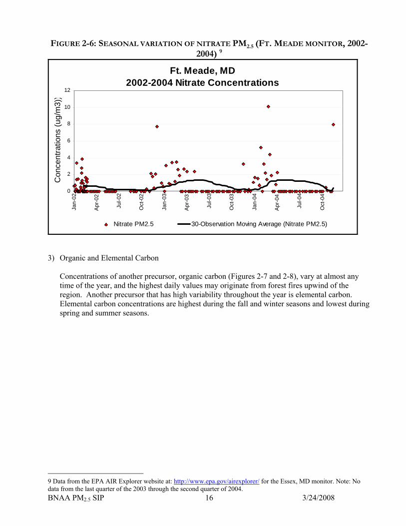
FIGURE 2-6: SEASONAL VARIATION OF NITRATE PM2.5 (FT. MEADE MONITOR, 2002-2004) 9

Ft. Meade, MD2002-2004 Nitrate Concentrations

0

2

4

6

8

10

12

Jan-

02

Apr

-02

Jul-0

2

Oct

-02

Jan-

03

Apr

-03

Jul-0

3

Oct

-03

Jan-

04

Apr

-04

Jul-0

4

Oct

-04

Con

cent

ratio

ns (u

g/m

3))

Nitrate PM2.5 30-Observation Moving Average (Nitrate PM2.5)

3) Organic and Elemental Carbon

Concentrations of another precursor, organic carbon (Figures 2-7 and 2-8), vary at almost any time of the year, and the highest daily values may originate from forest fires upwind of the region. Another precursor that has high variability throughout the year is elemental carbon. Elemental carbon concentrations are highest during the fall and winter seasons and lowest during spring and summer seasons.

BNAA PM2.5 SIP 3/24/2008 16



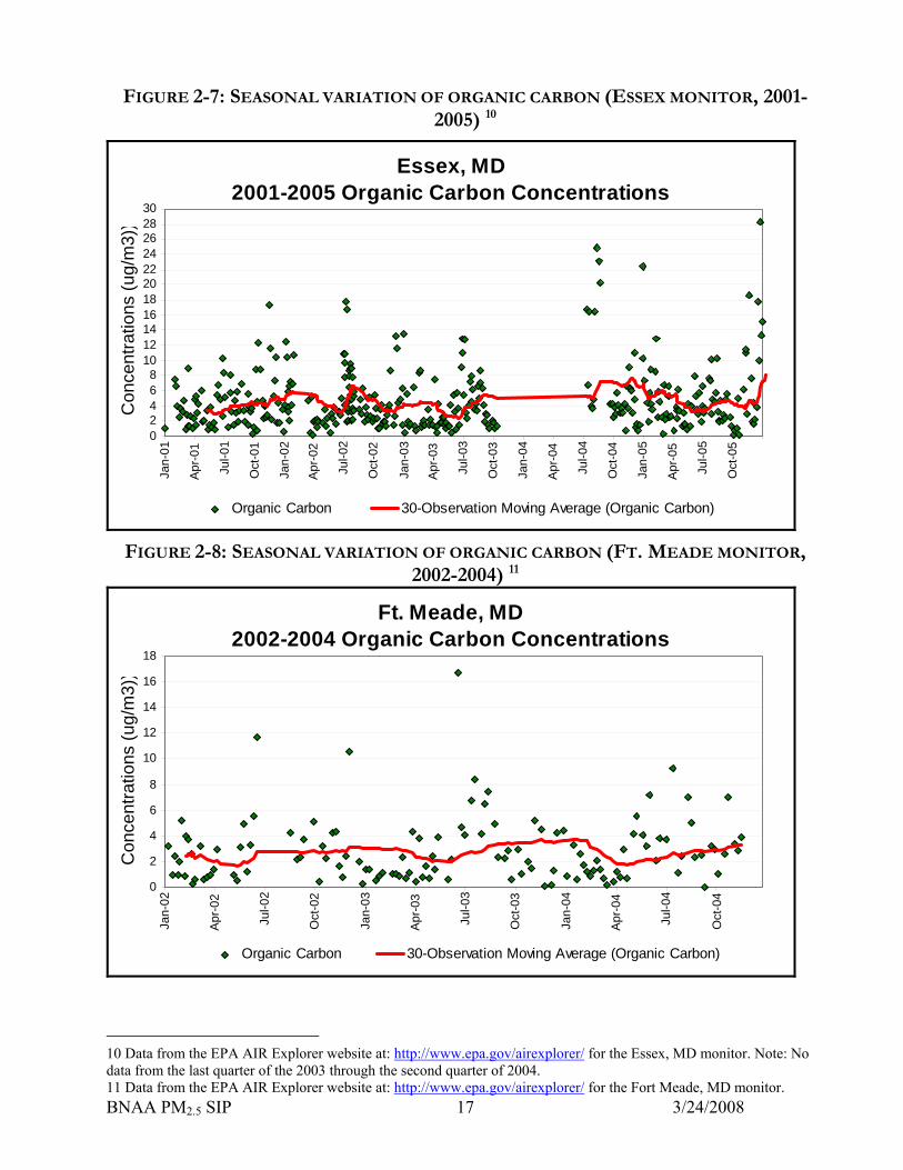
FIGURE 2-7: SEASONAL VARIATION OF ORGANIC CARBON (ESSEX MONITOR, 2001-2005) 10

Essex, MD2001-2005 Organic Carbon Concentrations

02468

1012141618202224262830

Jan-

01

Apr

-01

Jul-0

1

Oct

-01

Jan-

02

Apr

-02

Jul-0

2

Oct

-02

Jan-

03

Apr

-03

Jul-0

3

Oct

-03

Jan-

04

Apr

-04

Jul-0

4

Oct

-04

Jan-

05

Apr

-05

Jul-0

5

Oct

-05

Con

cent

ratio

ns (u

g/m

3))

Organic Carbon 30-Observation Moving Average (Organic Carbon)

FIGURE 2-8: SEASONAL VARIATION OF ORGANIC CARBON (FT. MEADE MONITOR, 2002-2004) 11

Ft. Meade, MD2002-2004 Organic Carbon Concentrations

0

2

4

6

8

10

12

14

16

18

Jan-

02

Apr

-02

Jul-0

2

Oct

-02

Jan-

03

Apr

-03

Jul-0

3

Oct

-03

Jan-

04

Apr

-04

Jul-0

4

Oct

-04

Con

cent

ratio

ns (u

g/m

3))

Organic Carbon 30-Observation Moving Average (Organic Carbon)





4) Ammonium

Ammonium concentrations vary seasonally according to whichever has higher concentrations; sulfates or nitrates. The chemicals that have higher concentrations are more available for chemical reactions than those with lower concentrations. Since during the summer, sulfates have much higher concentrations than other precursors, ammonia will typically react with the sulfates to produce ammonium sulfate, as in Figure 1. Hence, ammonium sulfates have higher concentrations in the summer (Figure 2-9 and 2-10), while ammonium nitrates have elevated concentrations in the winter due to heightened concentrations of nitrates available for chemical reactions with ammonia.

FIGURE 2-9: SEASONAL VARIATION OF AMMONIUM (ESSEX MONITOR, 2001-2005)

Essex, MD2002-2004 Ammonium Ion Concentrations

0

2

4

6

8

10

Jan-

01

Apr

-01

Jul-0

1

Oct

-01

Jan-

02

Apr

-02

Jul-0

2

Oct

-02

Jan-

03

Apr

-03

Jul-0

3

Oct

-03

Jan-

04

Apr

-04

Jul-0

4

Oct

-04

Jan-

05

Apr

-05

Jul-0

5

Oct

-05

Con

cent

ratio

ns (u

g/m

3))

Ammonium Ion 30-Observation Moving Average (Ammonium Ion)

BNAA PM2.5 SIP 3/24/2008 18

FIGURE 2-10: SEASONAL VARIATION OF AMMONIUM (FT. MEADE MONITOR, 2002-

2004) 12

Ft. Meade, MD2002-2004 Ammonium Ion Concentrations

0

2

4

6

8

Jan-

02

Apr

-02

Jul-0

2

Oct

-02

Jan-

03

Apr

-03

Jul-0

3

Oct

-03

Jan-

04

Apr

-04

Jul-0

4

Oct

-04

Con

cent

ratio

ns (u

g/m

3))

Ammonium Ion 30-Observation Moving Average (Ammonium Ion)

2.4 Diurnal Variation of Fine Particles Fine particle concentrations not only vary seasonally, but also diurnally, as shown in Figure 2-11 using hourly PM2.5 data between March 2003 and March 2007. Fine particle concentrations appear to be heightened during the morning and early evening hours, coinciding with peak traffic times for the Baltimore metropolitan area. A notable minimum in fine particle concentrations occurs during the late morning to early afternoon hours, presumably due to a diurnal increase in surface winds that help diffuse the particles about and away from the region. A lesser minimum also occurs during the overnight hours due to a strong reduction in mobile and industrial activity during sleeping hours.



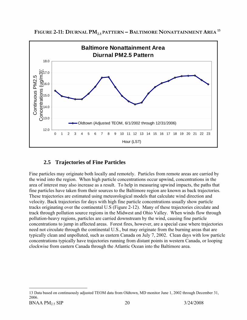
FIGURE 2-11: DIURNAL PM2.5 PATTERN – BALTIMORE NONATTAINMENT AREA 13

Baltimore Nonattainment AreaDiurnal PM2.5 Pattern

12.0

13.0

14.0

15.0

16.0

17.0

18.0

0 1 2 3 4 5 6 7 8 9 10 11 12 13 14 15 16 17 18 19 20 21 22 23

Hour (LST)

Con

tinuo

us P

M2.

5 C

once

ntra

tions

(ug/

m3)

)

Oldtown (Adjusted TEOM, 6/1/2002 through 12/31/2006)

2.5 Trajectories of Fine Particles Fine particles may originate both locally and remotely. Particles from remote areas are carried by the wind into the region. When high particle concentrations occur upwind, concentrations in the area of interest may also increase as a result. To help in measuring upwind impacts, the paths that fine particles have taken from their sources to the Baltimore region are known as back trajectories. These trajectories are estimated using meteorological models that calculate wind direction and velocity. Back trajectories for days with high fine particle concentrations usually show particle tracks originating over the continental U.S (Figure 2-12). Many of these trajectories circulate and track through pollution source regions in the Midwest and Ohio Valley. When winds flow through pollution-heavy regions, particles are carried downstream by the wind, causing fine particle concentrations to jump in affected areas. Forest fires, however, are a special case where trajectories need not circulate through the continental U.S., but may originate from the burning areas that are typically clean and unpolluted, such as eastern Canada on July 7, 2002. Clean days with low particle concentrations typically have trajectories running from distant points in western Canada, or looping clockwise from eastern Canada through the Atlantic Ocean into the Baltimore area.

BNAA PM2.5 SIP 3/24/2008 20

13 Data based on continuously adjusted TEOM data from Oldtown, MD monitor June 1, 2002 through December 31, 2006.

FIGURE 2-12a: PM FINE BACK TRAJECTORIES 14

FIGURE 2-12b: PM FINE BACK TRAJECTORIES 15

14 Based on data from April 2001 to December 2003 for Washington, D.C. – 5% Cleanest Days

BNAA PM2.5 SIP 3/24/2008 2115 Based on data from April 2001 to December 2003 for Washington, D.C. – 5% Dirtiest Days

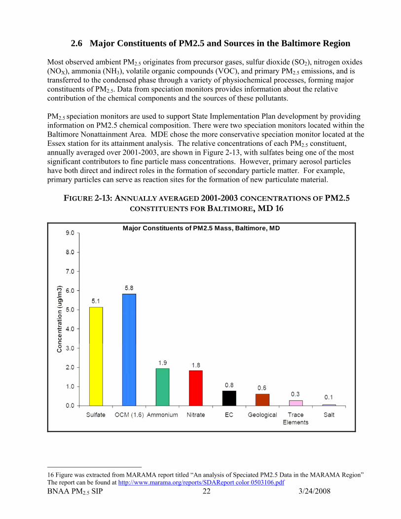
2.6 Major Constituents of PM2.5 and Sources in the Baltimore Region Most observed ambient PM2.5 originates from precursor gases, sulfur dioxide (SO2), nitrogen oxides (NOX), ammonia (NH3), volatile organic compounds (VOC), and primary PM2.5 emissions, and is transferred to the condensed phase through a variety of physiochemical processes, forming major constituents of PM2.5. Data from speciation monitors provides information about the relative contribution of the chemical components and the sources of these pollutants. PM2.5 speciation monitors are used to support State Implementation Plan development by providing information on PM2.5 chemical composition. There were two speciation monitors located within the Baltimore Nonattainment Area. MDE chose the more conservative speciation monitor located at the Essex station for its attainment analysis. The relative concentrations of each PM2.5 constituent, annually averaged over 2001-2003, are shown in Figure 2-13, with sulfates being one of the most significant contributors to fine particle mass concentrations. However, primary aerosol particles have both direct and indirect roles in the formation of secondary particle matter. For example, primary particles can serve as reaction sites for the formation of new particulate material.

FIGURE 2-13: ANNUALLY AVERAGED 2001-2003 CONCENTRATIONS OF PM2.5 CONSTITUENTS FOR BALTIMORE, MD 16

Major Constituents of PM2.5 Mass, Baltimore, MD

BNAA PM2.5 SIP 3/24/2008 22

16 Figure was extracted from MARAMA report titled “An analysis of Speciated PM2.5 Data in the MARAMA Region” The report can be found at http://www.marama.org/reports/SDAReport color 0503106.pdf

http://www.marama.org/reports/SDAReportcolor0503106.pdf

2.7 Sources of Fine Particles and Constituents Sources of fine particles include all types of combustion activities, including motor vehicle emissions, coal power plants, wood and vegetative burning, and certain industrial processes involving nitrates and sulfates. EPA uses the SANDWICH (Sulfate, Adjusted Nitrate, Derived Water, Inferred Carbon Hybrid) method to chemically characterize ambient PM2.5 speciation data. SANDWICH is a mass balance approach for estimating PM2.5 mass composition as if mass composition were measured by PM2.5 Federal Reference Monitors (FRM). This approach uses a combination of speciation measurements and modeled speciation estimates to represent FRM PM2.5 and is the default method in EPA modeling guidance to define baseline PM2.5 concentrations. Figures 2-14 and 2-15 show that a large portion of annual averaged PM2.5 composition consists of ammonium sulfate and ammonium nitrate, which are products of reactions of ammonia, sulfates, and nitrates in the atmosphere in summer and winter, respectively. Ammonia from sources such as fertilizer and animal feed operations contribute to the formation of ammonium sulfates and ammonium nitrates suspended in the atmosphere. The rest originates from sulfates, carbon and organic compounds from vegetative burning, coal power plants, geological dust, oil combustion, motor vehicle emissions, and diesel vehicle emissions. Nitrates usually originate from vehicle emissions and power generation.

FIGURE 2-14: PM2.5 COMPOSITION DATA FROM THE ESSEX, MD MONITOR 17

BNAA PM2.5 SIP 3/24/2008 23

17 PM2.5 composition data from Essex, MD monitor from 2001 – 2004. Total carbon and sulfates are dominant PM2.5 constituents in the Baltimore Nonattainment Area.

FIGURE 2-15: PM2.5 COMPOSITION DATA FROM THE FT. MEADE, MD MONITOR 18

2.8 Determination of Significance for Precursors EPA's PM2.5

implementation rule requires that state air agencies make a determination of the significance of PM2.5

pollutants/precursors for SIP planning purposes, including requirements for motor vehicle emission budgets for use in conformity. The significance of each precursor for PM2.5 has been analyzed and determined by EPA. Based on EPA’s advice, PM2.5-direct, SO2, and NOX were deemed significant for the Baltimore, Maryland non-attainment area, while ammonia (NH3) and other precursors were deemed insignificant at this time. According to EPA, sources of direct PM2.5 and SO2 must be evaluated for control measures in all non-attainment areas. Direct PM2.5 emissions include organic carbon, elemental carbon, and crustal material. If emissions of a precursor contribute significantly to PM2.5 concentrations in the area, then the sources of that precursor will need to be evaluated for reasonable control measures. EPA found sulfates and carbon to be the most significant fractions of PM2.5 mass in all non-attainment areas, and therefore concluded that the reductions in SO2 will lead to a significant net reduction in PM2.5 concentrations despite a potential slight increase in nitrates. The contribution of VOC to PM2.5 formation is the least understood of all precursors, and the reactions involving VOC are highly complex. In light of these factors, states are not required by EPA to address VOC as a PM2.5 attainment plan precursor and evaluate them for control measures, unless the state or EPA makes a finding that VOCs significantly contributes to PM2.5 concentrations

BNAA PM2.5 SIP 3/24/2008 24

18 PM2.5 composition data from Ft. Meade, MD monitor from 2002 – 2004. Total carbon and sulfates are dominant PM2.5 constituents in the Baltimore Nonattainment Area.

BNAA PM2.5 SIP 3/24/2008 25

in the non-attainment area or to other downwind air quality concerns. The Baltimore region decided to follow EPA’s advice on VOC. The role of ammonia in PM2.5 formation is also not as well understood as those of SO2 and carbon. Reducing ammonia emissions may marginally reduce PM2.5 concentrations, but particle and precipitation acidity may increase as a result. Increased acidity in particles and precipitation is a more adverse side effect of reducing ammonia concentrations, so ammonia is not required by EPA to be evaluated in this implementation plan unless deemed significant by the state or EPA. The Baltimore region decided to follow EPA’s advice on ammonia. The role of NOX in the formation of PM2.5 is very important. In the winter more NOx translates into increased amounts of hydrogen nitrate (HNO3) and Ammonia Nitrate (NH4NO3), favored by the availability of ammonia, low temperatures, and high relative humidity. PM2.5 concentrations will respond most effectively to NOx reductions in the winter by reducing the amounts of hydrogen nitrate (HNO3) and Ammonia Nitrate (NH4NO3) in the atmosphere that can form PM2.5. Therefore, states are required to address NOX as a PM2.5 attainment plan precursor and evaluate reasonable controls for nitrates in implementation plans. Therefore, states are required to address NOX as a PM2.5 attainment plain precursor and evaluate reasonable controls for nitrates in implementation plans, unless it is found by the EPA that NOX emissions from sources in the state do not significantly contribute to the PM2.5 concentrations in the non-attainment area. The Baltimore region decided to follow EPA’s advice on NOX. EPA's PM2.5 implementation rule requires that state air agencies make a determination of the significance of PM2.5 pollutants/precursors for SIP planning purposes, including requirements for motor vehicle emission budgets for use in conformity. The known PM pollutants include PM2.5 direct as well as the precursors NOX, SO2, VOC, and ammonia (NH3) (see Table 4). PM2.5 direct and the precursors NOX and SO2 are deemed significant under the EPA guidance. PM10 is required for the base year emission inventory, but does not need to be included in the SIP control strategy. Several precursors are presumed to be insignificant and do not need to be included in the SIP control strategy unless the state or EPA makes a finding of significance. Table 2-1 summarizes the federal requirements for each precursor. Table 2-1: EPA SIP Requirements for PM Pollutants

PM2.5 Direct NOx SO2 VOC NH3 PM10

Base Year Emission Inventory √ √ √ √ √ √

SIP Controls √ √ √ - - Not required

Summary of Significance Determinations for PM Pollutants Through interagency consultation and consideration of available information, the state air agencies have completed significance determinations for each of the PM precursors. The determination was conducted using a two-step process. Step 1 involved determining whether PM pollutants/precursors are considered significant for SIP planning purposes. Step 2 involved determining whether PM pollutants/precursors identified as significant in Step 1 require Motor Vehicle Emission Budgets (MVEBs) for conformity. Table 2-2 summarizes the determination.

BNAA PM2.5 SIP 3/24/2008 26

Table 2-2: Summary of Significance Determinations for SIP Controls and Motor Vehicle Emission Budgets

PM Direct NOx SO2 VOC NH3

Step 1: Determine Significance for SIP Controls √ √ √ No No

Step 2: Determine Significance for Establishing Motor Vehicle Emission Budgets for Conformity √ √ No No No

EPA notes that any significance or insignificance finding made prior to EPA’s adequacy finding for budgets in a SIP, or EPA’s approval of the SIP, should not be viewed as the ultimate determination of the significance of precursor emissions in a given area. State and local agencies may reconsider significance findings based on information and analyses conducted as part of the SIP development process. Determine Significance for SIP Controls The only precursors for which significance determinations are needed for SIP control purposes are VOC and ammonia. EPA requires that PM2.5 direct, NOX, and SO2 controls be evaluated and included in the SIP. A primary factor considered for VOC and ammonia is that the region is already showing attainment of the PM2.5 annual NAAQS so no additional controls are needed for attainment purposes. A second factor considered is that EPA guidance allows states to presume that these precursors are insignificant unless modeling or other analysis indicates that the precursor should be considered significant. A summary of the rationale for the significance determinations for VOC and ammonia is listed in Table 2-3. Table 2-3: Summary of Rationale for VOC and NH3 Insignificance Determinations for SIP Controls

Pollutant Criteria

VOC NH3

Are emission controls needed for attainment or maintenance? No No

Is there evidence to counter EPA's presumption that the precursor be considered insignificant? No No

Will reducing emissions of the precursor have a significant impact on PM2.5 concentrations?

No, based on VISTAS* modeling

No, based on VISTAS modeling

Are technology options available to control emissions? Yes Varies by source

Is the precursor considered significant for SIP Planning purposes? No No

* VISTAS is the Visibility Improvement - State and Tribal Association of the Southeast National research is underway to assess the contribution of VOCs to secondary organic aerosol formation. States are following the research and will reconsider the significance determination for VOCs when further technical information becomes available.

BNAA PM2.5 SIP 3/24/2008 27

3.0 THE 2002 BASE-YEAR INVENTORY

3.1 Background and requirements The 2002 Base-Year Inventory is published in a separate document, "2002 Base Year Emissions Inventory & QA/QC Plan Maryland," (June 15, 2006). This document was submitted to EPA Region III. This document was prepared the Maryland Department of the Environment. It is available for inspection at the Air and Radiation Management Administration, 1800 Washington Boulevard, Suite 730, Baltimore, Maryland 21230. Relevant portions of this document including, source category listings and descriptions, methods and data sources, emission factors, controls, spatial and temporal allocations, and example calculations are included in Appendix A1. The full inventory document titled, 2002 Base-Year Emissions Inventory of PM2.5 Precursor Emissions, is attached to this SIP document in Appendix A. The emissions inventory covers all Maryland nonattainment areas, Figure 1-1, which are classified as moderate nonattainment areas for particulate matter by the U.S. Environmental Protection Agency (EPA). The 2002 emissions inventory is the starting point for calculating the emissions reduction requirement needed to meet the requirements prescribed for moderate nonattainment areas by the Clean Air Act Amendments and EPA. Appendix A (2002 Base Year Emissions Inventory of PM2.5 Precursor Emissions for the Baltimore, MD Nonattainment Area) of the Annual PM2.5 SIP document addresses emissions of PM2.5-Primary, oxides of nitrogen (NOX), sulfur dioxide (SO2), volatile organic compounds (VOCs), ammonia (NH3), and PM10-Primary on an annual basis. Included in the inventory are anthropogenic (man-made) sources, such as, point, area, non-road and on-road mobile sources and biogenic (naturally occurring) sources of PM2.5 precursors. The 2002 base-year annual inventories for PM2.5-PRI, NOX, SO2, VOC, NH3, and PM10-PRI are summarized in Table 3-1.

Table 3-1: 2002 Base-Year Annual Inventory

(Tons/Year)

NH3 NOx PM2.5-PRI PM10-PRI SOx VOC Total

Point 183.92 40,280.02 3,047.60 4,441.99 97,909.52 3,463.14 149,326.19 Quasi-Point 0.00 2,966.26 320.30 421.90 1,965.68 416.57 6,090.71

Area 3,553.54 7,372.61 8,460.36 31,108.52 4,962.88 40,654.48 96,112.39 Non-Road 11.25 14,077.13 1,525.44 1,586.41 1,202.93 17,521.85 35,925.01 On-Road 2,460.86 66,229.56 1,080.35 1,522.33 2,161.95 25,823.92 99,278.97 Biogenics 0.00 635.56 0.00 0.00 0.00 33,527.27 34,162.83

Total 6,209.57 131,561.14 14,434.05 39,081.15 108,202.96 121,407.23 420,896.10 * Small discrepancies may result due to rounding

BNAA PM2.5 SIP 3/24/2008 28

3.2 Total Emissions by Source

3.2.1 Point Sources For emissions inventory purposes, point sources are defined as stationary, commercial, or industrial operations that emit more than 10 tons per year (tons/year) of VOCs or 25 tons/year or more of NOx or CO. The point source inventory consists of actual emissions for the base-year 2002 and includes sources within the geographical area of the Baltimore Nonattainment Area. For source category listings and descriptions, methods and data sources, emission factors, controls, spatial and temporal allocations, and example calculations please refer to Appendix A1. For Base-Year Emission Inventory data please refer to Appendix A2.

3.2.2 Quasi-Point Sources The Maryland Department of the Environment Air and Radiation Management has identified several facilities that due to size and/or function are not considered point sources. These establishments contain a wide variety of air emission sources, including traditional point sources, on-road mobile sources, off-road mobile sources and area sources. For each particular establishment, the emissions from these sources are totaled under a single point source and summary documents include these “quasi-point” sources as point sources. Quasi-point sources will include all emissions at the facility regardless of whether they are classified as point, area, nonroad, or mobile source emissions. These emissions are actual emissions reported for the facilities. The Baltimore Nonattainment Area has the following Quasi-point sources:

• Baltimore Washington International Airport (BWI) • Aberdeen Proving Grounds

These emissions have been included as Point Source in summary documents. For source category listings and descriptions, methods and data sources, emission factors, controls, spatial and temporal allocations, and example calculations please refer to Appendix A1. For Base-Year Emission Inventory data please refer to Appendix A3.

3.2.3 Area Sources Area sources are sources of emissions too small to be inventoried individually and which collectively contribute significant emissions. Area sources include smaller stationary point sources not included in the states' point source inventories such as printing establishments, dry cleaners, and auto refinishing companies, as well as non-stationary sources. Area source emissions typically are estimated by multiplying an emission factor by some known indicator of collective activity for each source category at the county (or county-equivalent) level. An activity level is any parameter associated with the activity of a source, such as production rate or fuel consumption that may be correlated with the air pollutant emissions from that source. For example, the total amount of VOC emissions emitted by commercial aircraft can be calculated by

BNAA PM2.5 SIP 3/24/2008 29

multiplying the number of landing and takeoff cycles (LTOs) by an EPA-approved emission factor per LTO cycle for each specific aircraft type. Several approaches are available for estimating area source activity levels and emissions. These include apportioning statewide activity totals to the local inventory area and using emissions per employee (or other unit) factors. For example, solvent evaporation from consumer and commercial products such as waxes, aerosol products, and window cleaners cannot be routinely determined for many local sources. The per capita emission factor assumes that emissions in a given area can be reasonably associated with population. This assumption is valid over broad areas for certain activities such as dry cleaning and small degreasing operations. For some other sources an employment based factor is more appropriate as an activity surrogate. For source category listings and descriptions, methods and data sources, emission factors, controls, spatial and temporal allocations, and example calculations please refer to Appendix A1. For Base-Year Emission Inventory data please refer to Appendix A4.

3.2.4 Mobile Sources On-road mobile sources include all vehicles registered to use the public roadways. The predominant emission source in this category is the automobiles, although trucks and buses are also significant sources of emissions. The computation of highway vehicle emissions required two primary entities: a) vehicle emission factors and b) vehicle activity. The Emission factors are generated by using the latest version of U.S. EPA’s emission factor model MOBILE6.2. Vehicle activity (vehicle miles traveled – termed VMT for short) is usually obtained from two sources: a) State Highway Administration (SHA), and b) Baltimore Metropolitan Council (BMC). VMT data from SHA, based on vehicle traffic counts on the roadway system, is mainly used for the rural counties. The BMC-provided transportation modeled link-based data is used in the emission modeling of the Baltimore Nonattainment Area as mandated by the CAAA 1990. In a simple modeling scenario, the product of emission factor and vehicle miles traveled should yield emission levels for that scenario. Proper units and conversion are used to arrive at reasonable emission estimates. In a complex modeling scenario many types of emissions such as exhaust, evaporative, diurnal, crankcase, refueling, etc., emissions are computed separately and treated with the appropriate activity levels to yield a complex model result. MOBILE6 expects enormous amount of local data input such as the fleet characteristics, fleet mileage accrual rates, speed, fuel parameters, inspection and maintenance (I/M) program in place, weather data, and so on. In MOBILE6 emission factor model, the total highway vehicle population is characterized by the following 16 composite vehicle type categories:

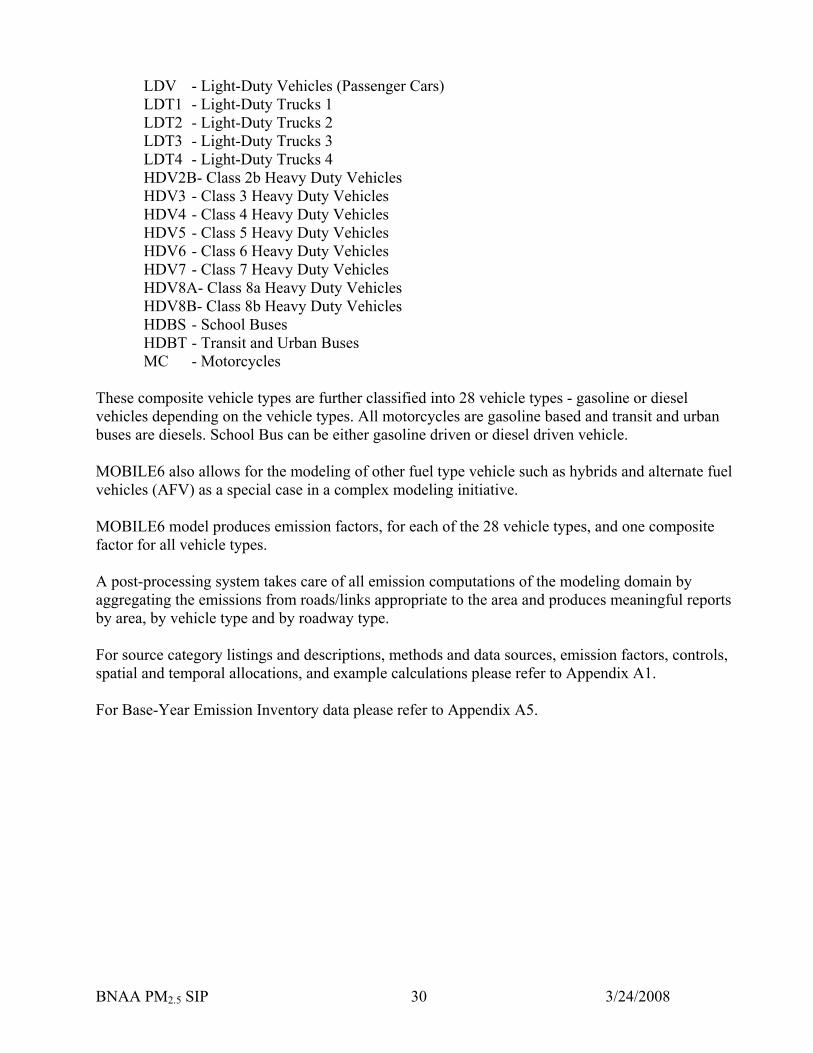
BNAA PM2.5 SIP 3/24/2008 30

LDV - Light-Duty Vehicles (Passenger Cars) LDT1 - Light-Duty Trucks 1 LDT2 - Light-Duty Trucks 2 LDT3 - Light-Duty Trucks 3 LDT4 - Light-Duty Trucks 4 HDV2B- Class 2b Heavy Duty Vehicles HDV3 - Class 3 Heavy Duty Vehicles HDV4 - Class 4 Heavy Duty Vehicles HDV5 - Class 5 Heavy Duty Vehicles HDV6 - Class 6 Heavy Duty Vehicles HDV7 - Class 7 Heavy Duty Vehicles HDV8A- Class 8a Heavy Duty Vehicles HDV8B- Class 8b Heavy Duty Vehicles HDBS - School Buses HDBT - Transit and Urban Buses MC - Motorcycles

These composite vehicle types are further classified into 28 vehicle types - gasoline or diesel vehicles depending on the vehicle types. All motorcycles are gasoline based and transit and urban buses are diesels. School Bus can be either gasoline driven or diesel driven vehicle. MOBILE6 also allows for the modeling of other fuel type vehicle such as hybrids and alternate fuel vehicles (AFV) as a special case in a complex modeling initiative. MOBILE6 model produces emission factors, for each of the 28 vehicle types, and one composite factor for all vehicle types. A post-processing system takes care of all emission computations of the modeling domain by aggregating the emissions from roads/links appropriate to the area and produces meaningful reports by area, by vehicle type and by roadway type. For source category listings and descriptions, methods and data sources, emission factors, controls, spatial and temporal allocations, and example calculations please refer to Appendix A1. For Base-Year Emission Inventory data please refer to Appendix A5.

BNAA PM2.5 SIP 3/24/2008 31

3.2.5 Nonroad Sources Emissions for all nonroad vehicles and engines except airport (aircraft, ground support equipment (GSE) and, auxiliary power units (APU)), locomotives, and diesel marine vessels were calculated using EPA’s NONROAD2005.0.0 (dt. 12/02/2005) model. Since the time it was first issued on 12/02/2005, this model version underwent several corrections. The base year nonroad inventory was created using the version current as of 3/21/2006. Emissions from the “nonroad vehicles and engines” category result from the use of fuel in a diverse collection of vehicles and equipment, including vehicles and equipment in the following categories:

• Recreational vehicles, such as all-terrain vehicles and off-road motorcycles; • Logging equipment, such as chain saws; • Agricultural equipment, such as tractors; • Construction equipment, such as graders and back hoes; • Industrial equipment, such as fork lifts and sweepers; • Residential and commercial lawn and garden equipment, such as leaf and snow blowers. • Aircraft ground support equipment.

The nonroad model estimates emissions for each specific type of nonroad equipment by multiplying the following input data estimates:

• Equipment population for base year (or base year population grown to a future year), distributed by age, power, fuel type, and application;

• Average load factor expressed as average fraction of available power; • Available power in horsepower; • Activity in hours of use per year; and • Emission factor with deterioration and/or new standards.

The emissions are then temporally and geographically allocated using appropriate allocation factors. Aircraft (military, commercial, general aviation, and air taxi) and auxiliary power units (APU) operated at airports along with locomotives and diesel marine vessels are also considered nonroad sources and are included in the nonroad category. Baltimore Washington International Airport (BWI) and the Maryland Aviation Administration (MAA) provided all types of airport emissions for the airport. The Maryland Port Authority provided data for commercial marine vessels entering the Chesapeake Bay. Emissions from locomotives and commercial diesel marine vessels were calculated my MDE engineers. For source category listings and descriptions, methods and data sources, emission factors, controls, spatial and temporal allocations, and example calculations please refer to Appendix A1. For Base-Year Emission Inventory data please refer to Appendix A6.

BNAA PM2.5 SIP 3/24/2008 32

3.2.6 Biogenic Emissions An important component of the inventory is biogenic emissions. Biogenic emissions are those resulting from natural sources. Biogenic emissions are primarily VOCs that are released from vegetation throughout the day. Biogenic emissions of NOx include lightning and forest fires. EPA used a biogenic computer model (BEIS3.12) to estimate biogenic emissions for each county in the country for all twelve months of the year 2002. Emissions data for Baltimore Nonattainment area was acquired from the EPA website (ftp://ftp.epa.gov/EmisInventory/2002finalnei/biogenic_sector_data/). EPA has recommended that states use these emissions in case they do not have their own estimated biogenic emissions. Baltimore, MD particulate matter non-attainment area decided to use the inventories provided by the EPA.

BNAA PM2.5 SIP 3/24/2008 33

4.0 THE 2009 PROJECTED UNCONTROLLED AND CONTROLLED INVENTORIES

Projected uncontrolled and controlled inventories for the attainment year 2009 are required for the region to calculate benefits from various control measures. Comparison of the base year 2002 and the attainment year 2009 controlled inventories provides a trend in emissions between these two milestone years. Also, the base year 2002 and the attainment year 2009 controlled inventories are required for emissions reduction calculation to meet attainment contingency requirements. The 2002 Base Year Inventory is described in Chapter 3. This chapter presents the 2009 projected uncontrolled and controlled inventories, the estimation of the levels of emissions in that year before and after the consideration of emissions controls respectively The projected inventories are derived by applying the appropriate growth factors to the 2002 Base-Year Emissions Inventory. EPA guidance describes four typical indicators of growth. In order of priority, these are product output, value added, earnings, and employment. Surrogate indicators of activity, for example population growth, are also acceptable methods. Round 6B Cooperative Forecasting results (population, household and employment projections), prepared and officially adopted by the Baltimore Metropolitan Council (BMC) were used to project emissions from area sources. Projections for onroad emissions were developed using MOBILE6.2 (January 2003) model (please see Appendix C for information on mobile source emissions). EPA’s nonroad model, NONROAD2005, was used for developing both 2008 and 2009 nonroad model inventories. BMC’s Round 6B Cooperative Forecasting results and the Economic Growth Analysis System (EGAS) model was used to project growth in the additional nonroad source categories such as railroad locomotives, marine vessels and airports. The Economic Growth Analysis System (EGAS) model was used to project growth in point source emissions.

4.1 Growth Projection Methodology The following sections describe the method followed to determine the projected inventories for 2009.

4.1.1 Growth Projection Methodology for Point Sources: EGAS The growth in point source emissions is projected using EGAS version 5.0. Point source emissions for 2002 are provided from the state data sources and the model is run with the following options selected: projections are run by Source Classification Code; the Bureau of Labor Statistics national economic forecast; and the baseline regional economic forecast. For source category listings and descriptions, projection methods and data sources, and surrogate growth indicators please refer to Appendix B1. Point source emission projection data is contained in Appendix A2

BNAA PM2.5 SIP 3/24/2008 34

4.1.2 Growth Projection Methodology for Quasi-Point Sources Quasi-point sources will include all emissions at the facility regardless of whether they are classified as point, area, nonroad, or mobile source emissions. These emissions are actual emissions reported for the facilities. Actual emissions will be forecast to the projection years using surrogates specific to each quasi-point source. The growth factor indicators and their sources are listed below by facility:

Quasi-Point Source Surrogate Growth Indicator

Baltimore Washington International Airport (BWI)

Aircraft LTOs FAA Aircraft Operations Forecasts

Mobile Source Emissions FAA Enplanement Forecasts

Aberdeen Proving Grounds BRAC Population Estimates For source category listings and descriptions, projection methods and data sources, and surrogate growth indicators please refer to Appendix B1. Quasi-point source emission projection data is contained in Appendix A3.

4.1.3 Growth Projection Methodology: Area Sources Base-year area source surrogate growth factors for 2002 were calculated using 2002 population, household, and employment data. Linearly interpolating between 2002 and 2005 data produced the 2002 data. Dividing Round 6B population, household, and employment forecasts for the analysis year by the derived 2002 values for the region produced the growth factors for the periods of 2002 to 2008 and 2002 to 2009. Categories related to transport and storage of gasoline were grown using projected vehicle miles traveled (VMT) for analyses years. Area projection inventories are contained in Appendix B. The growth factors used for the 2008 and 2009 projection years are presented in Tables 4-1 and 4-2. The growth factors were applied to emissions categories by specific jurisdictions.

Table 4-1: 2002-2009 Area Source Growth Factors Jurisdiction

Employment 2

Population

2

Household

2

VMT 3

Anne Arundel County 1.0857 1.0508 1.0848 1.1580

Baltimore City 1.0639 1.0109 1.1310 1.1400

Baltimore County 1.1566 1.0586 1.0677 1.1407

Carroll County 1.1030 1.1220 1.1352 1.1605

Harford County 1.1667 1.1141 1.1399 1.1637

Howard County 1.0289 1.1161 1.1310 1.1400

BNAA PM2.5 SIP 3/24/2008 35

The 2009 emissions for area sources were calculated by multiplying the 2002 base-year area emissions by the above growth factors for the appropriate year for each jurisdiction. Each area source category was matched to an appropriate growth surrogate based on the activity used to generate the base-year emission estimates. Surrogates were chosen as follows: Surface Coating – depending on whether emission factors were based on employment or population, surrogate chosen varied with individual sub-categories. For example, automobile refinishing category was grown using employment as the emission factor was based on it, but population was chosen for growing traffic markings as its emission factor was based on population. Commercial/Consumer Solvent Use - population was chosen as the growth surrogate since 2002 emissions are based on per capita emission factors. Residential Fuel Combustion – households was chosen as the growth surrogate. Industrial/Commercial/Institutional Fuel Combustion - employment was chosen as the growth surrogate except for the commercial/institutional coal combustion category, where no growth was assumed. Vehicle Fueling (Stage II) and Underground Tank Breathing - all gasoline marketing categories were based on vehicle miles traveled (VMT) data since VMT is an appropriate surrogate for gasoline sales. Emission factors for these categories are based on gasoline sales. Open Burning - population was chosen as the growth surrogate as yard wastes, land debris, etc. increase with population. Structural Fires, Motor Vehicle Fires – population was chosen as the growth surrogate. Publicly Owned Treatment Works (POTW) – households was chosen as the growth surrogate. Dry Cleaning - population was chosen as the surrogate. Graphic Arts - population was used to estimate growth since emissions are based on per capita emission factors. Surface Cleaning - employment growth was used as the surrogate. Tank Truck Unloading –growth in VMT was applied to this category since base-year emissions are calculated using gasoline sales. Municipal Landfills - Base-year emissions are estimated using data on total refuse deposited. Population was chosen as a surrogate since deposited waste is from the general population rather than industrial facilities. Asphalt Paving - population was chosen as the surrogate since base-year emissions are calculated using per capita emission factors. Bakeries, Breweries - population was chosen as the surrogate.

BNAA PM2.5 SIP 3/24/2008 36

Soil/Groundwater Remediation - zero growth was applied to this category. The number of remediations during the any season, used to generate base-year emissions, does not directly correlate to population, households, or employment growth. General Aviation and Air Taxi Emissions - Emissions from small airports were projected using the EGAS 5.0 model. The Maryland Aviation Administration (MAA) provided commercial aircraft operations at Baltimore Washington International (BWI) Airport. Emissions were calculated using FAA-approved activity data and the Emissions Dispersion Modeling system (EDMS) model. Emissions were grown by FAA Terminal Area Forecasts (TAFs). Aircraft Refueling Emissions - emissions from refueling of aircrafts was projected based on employment. Portable Fuel Container Emissions - emissions from portable fuel containers were grown based on population. Railroad Locomotives - employment growth was used as the surrogate. Forest Fires, Slash Burning, Prescribed Burning – zero growth was applied to this category. Accidental Oil Spills - zero growth was applied to this category. Incineration– zero growth was applied to this category. Pesticide Application - zero growth was applied to this category. For source category listings and descriptions, projection methods and data sources, and surrogate growth indicators please refer to Appendix B1. Area source emission projection data is contained in Appendix A4.

4.1.4 Growth Projection Methodology: Nonroad Model Sources The 2009 projected uncontrolled nonroad source inventory was created through the use of EPA’s NONROAD2005 model version 2005a (February 8, 2006), except for locomotives, aircrafts, and aircraft auxiliary power units. This model was run with its associated graphic user interface NONROAD2005.1.0 (June 12, 2006), reporting utility version. 2005c (March 21, 2006), and all geographical allocation data files updated until February 1, 2006. The base year 2002 nonroad source inventory was also created using the same model, reporting utility, geographical allocation data files, and graphic user interface versions. A four-season approach was adapted for developing annual emissions. The NONROAD2005 model was run for the metropolitan Baltimore region for the four seasons (winter, spring, summer, and autumn) and then seasonal emissions were summed up to get the annual emissions. The four seasons considered were Winter (December, January, and February), Spring, (March, April, and May), Summer (June, July, and August), and Autumn (September, October, and November). Model inputs (temperature, fuel, and other parameters) were prepared for the four seasons used for annual model runs and are provided in the Appendix A along with the details of methodology used

BNAA PM2.5 SIP 3/24/2008 37

to develop those inputs. For projected 2009 uncontrolled inventory, all nonroad model inputs valid for the base year 2002 were used, the technology limiter was set at the 2002 and the growth assumptions valid for the year 2009 were used. The methodology to prepare inputs for the summer season is provided below.

Temperature: Temperature data was acquired from the National Climatic Data Center (NCDC). Hourly average temperature data were collected for Baltimore Washington International (BWI) station for the top ten 8-hour maximum ozone days between 2002-2004. Then minimum, maximum, and average temperatures were computed from this hourly temperature dataset.

Fuel inputs:

Month specific data for fuel RVP and oxygen weight percent were collected from BRTB19 and their staff, BMC20 and MDE Mobile Source Division. The data was averaged for the period to get seasonal average inputs. Model defaults were used for gas, diesel, marine diesel, and CNG/LPG sulfur percent. Stage II controls of zero percent was assumed for the model runs.

The model inputs (temperature, fuel, and other parameters) for 2009 are listed below:

Table 4-2: 2009 NONROAD Model Inputs Parameters 2009 Values Min. Temperature 65.55 Max. Temperature 87.6 Avg. Temperature 76.8 Reid Vapor Pressure (RVP) 6.6 Gas Sulfur (%) 0.003 Diesel Sulfur (%) 0.0348 Marine Diesel Sulfur (%) 0.0408 CNG/LPG Sulfur (%) 0.003 Oxygen Weight (%) 2.0 Stage II Control (%) 0

Since the nonroad model does not generate emissions for aircraft, APU, locomotives, and commercial diesel marine vessels, these were either projected from the base year emissions using the BMC Round 6B Cooperative Forecast or the EGAS model. Below are the details for projecting emissions for the above mentioned individual nonroad categories.

19 Baltimore Regional Transportation Board 20 Baltimore Metropolitan Council

BNAA PM2.5 SIP 3/24/2008 38

4.1.5 Growth Projection Methodology: Nonroad Sources

Aircraft emissions (military, commercial, general aviation, air taxi) Maryland Aviation Administration (MAA) provided all types of airport activity data and emissions for Baltimore Washington International (BWI) airport. Aviation emissions from BWI were grown by FAA Terminal Area Forecasts (TAFs). Emissions were calculated using FAA-approved activity data and the Emissions Dispersion Modeling system (EDMS) model. General aviation and air taxi emissions from small airports were projected using the EGAS 5.0 model.

Auxiliary power units emissions These emissions were only available for Baltimore Washington International (BWI) airport. Emissions were calculated using FAA-approved activity data and the Emissions Dispersion Modeling system (EDMS) model.

Ground support equipment emissions

The NONROAD2005.1.0 model generated these emissions for small airports. BWI GSE emissions were generated using the EDMS model, which calculated emissions based on actual aircraft operations. The Nonroad model calculates emissions based on GSE population only and therefore emissions generated this way are considered less accurate than the one generated by the EDMS model.

Commercial Diesel Marine Vessels Base year emissions from commercial diesel marine vessels were grown to future years using employment as the surrogate. Railroad Railroad or locomotive emissions were grown using employment as the surrogate. For source category listings and descriptions, projection methods and data sources, and surrogate growth indicators please refer to Appendix B1. Nonroad mobile source emission projection data is contained in Appendix A6.

4.1.6 Growth Projection Methodology: Onroad Sources The 2009 mobile source inventories were created through the use of several modeling including Mobile6.2 and the Highway Performance Monitoring System (HPMS). A full description of this mobile emission estimating process can be found in Appendix C of this report.

4.1.7 Biogenic Emission Projections Biogenic emission inventories for 2009 are the same as those used for the 2002 base year for Baltimore, MD nonattainment region. Year specific biogenic inventories for 2009 were not estimated. 2002 base year emissions were estimated by EPA using BEIS3.12 model.

BNAA PM2.5 SIP 3/24/2008 39

4.2 Offset Provisions, Emission Reduction Credits and Point Source Growth

The Act requires that emission growth from major stationary sources in nonattainment areas be offset by reductions that would not otherwise be achieved by other mandated controls. The offset requirement applies to all new major stationary sources and existing major stationary sources that have undergone major modifications. Increases in emissions from existing sources resulting from increases in capacity utilization are not subject to the offset requirement. For the purposes of the offset requirement, major stationary sources include all stationary sources exceeding an applicable size cutoff. The NSR thresholds for the Baltimore nonattainment area are 10 tpy VOC and 25 tpy NOx. EPA has issued guidance on the inclusion of emission reduction credits in the projected emissions inventory. The guidance states “The base year inventory includes actual emissions from existing sources and would not normally reflect emissions from units that were shutdown or curtailed before the base year (2002), as these emissions are not “in the air” for purposes of demonstrating attainment, they must be specifically included in the projected emissions inventory used in the attainment demonstration along with other growth in emission over the base year inventory. This step assures that emissions from shutdown and curtailed units are accounted for in attainment planning.” 21 MDE has included emission reduction credits in the attainment demonstration projected inventory. A list of these emission reduction credits and associated facilities is shown in Table 4.3.

Table 4.3: Emission Reduction Credits

Facility Name

State Facility Identifier

Pollutant Code

Emission Reduction Credits (TPY)

Bethlehem Steel 005-0147 NOX 701Pulaski Incinerator 510-0498 NOX 302Quebecor Printing 003-0274 NOX 2G. Heileman Brewing (Strohs) 005-0129 NOX 24Grief Brothers Corp. 005-0134 NOX 1U.S.Can - Sparrows Pt. (Amer Nat) 005-0183 NOX 7TPS Technologies, Inc. -Todd's La. 005-2131 NOX 16Simpkins Industries - River Rd 027-0005 NOX 87General Electric 027-0020 NOX 82Alltrista Metal Services 510-0508 NOX 2Trigen (Leadenhall St) 510-2796 NOX 33Chevron Asphalt 510-0072 NOX 49Coca Cola 510-0242 NOX 5Crown Cork & Seal - Duncanwood 510-0320 NOX 10Gordon D. Garratt 510-0360 NOX 1Proctor & Gamble 510-0185 NOX 12Schluderberg-Kurdle 510-0283 NOX 19

21 Federal Register/Vol. 71, No. 243/ Tuesday, December 19, 2006/ Proposed Rules

BNAA PM2.5 SIP 3/24/2008 40

Facility Name


Pollutant Code


(Westport 510-0006 & Riverside 005-0078) 510-0006 NOX 1480Giant - Bakery (930 King St) 031-0224 NOX 2Armco Stainless/ 510-0340 NOX 16Bausch & Lomb 023-0019 NOX 1Rohr Industries 043-0104 NOX 6Showell Farms 047-0036 NOX 8WR Grace 510-0076 NOX 17General Motors - Truck & Bus 510-0354 NOX 119Andrews Air Force Base 033-0655 NOX 15Millenium Inorganic Chemicals 510-0109 NOX 30Quebecor Printing 003-0274 VOC 322Bethlehem Steel 005-0147 VOC 0Pulaski Incinerator 510-0498 VOC 11BARCO - Fairlawn 510-2854 VOC 5Crown Cork & Seal - Duncanwood 510-0320 VOC 13Giant - Bakery - 930 King St 031-0224 VOC 0Cello Professional Products 025-0145 VOC 0Grief Brothers Corporation 005-0134 VOC 0General Motors - Truck & Bus 510-0354 VOC 0General Motors - Electromotive 005-0692 VOC 15Crown Central Petroleum 003-0234 VOC 21BGE - SNG Plant 005-1054 VOC 7Ecko-Glaco Ltd. 005-0310 VOC 27G. Heileman Brewing Co. (Strohs) 005-0129 VOC 48Maryland Paper Box 005-2220 VOC 15Schlumberger Malco, Inc. 005-1614 VOC 12U.S.Can-Sparrows Pt. (Amer Nat) 005-0183 VOC 90TPS Technologies (Todd's La.) 005-2131 VOC 4Simpkins Industries (River Rd) 027-0005 VOC 73M Commercial Graphics 013-0052 VOC 30Blue Chip Products 015-0058 VOC 35Baycraft Fiberglass Engineering 025-0231 VOC 10Alltrista Metal Services 510-00508 VOC 11Armco/Balto. Specialty Steel 510-0340 VOC 11CE Stevens Packaging (printer) 510-2900 VOC 10Chevron Asphalt 510-0072 VOC 2Conoco Sun Gasoline Terminal 510-0676 VOC 27Bata Shoe 025-0003 VOC 18Cherokee Sanford 033-0565 VOC 0PPG Industries 001-0005 VOC 28Tidewater Industrial Corp. 011-0039 VOC 11Crown Cork & Seal - Hurlock 019-0073 VOC 96

BNAA PM2.5 SIP 3/24/2008 41

Facility Name


Pollutant Code


Mail-Weil Graphics 019-0097 VOC 8Metalfab - Grove Road 021-0317 VOC 11Bausch & Lomb 023-0019 VOC 16American Mouldings 043-0191 VOC 69Carpenter Insulation 043-0189 VOC 146CSX Minerals 043-0110 VOC 10Rohr Industries 043-0104 VOC 4Constellation - Westport 510-0006 & Riverside 005-0078 510-0006 VOC 23Thomas Mfg. 005-0240 VOC 22LeSaffre Yeast 510-0191 VOC 179

4.3 Actual vs. Allowable Emissions in Development of the 2009 Projected Emissions Inventories

For the purposes of calculating 2009 projection emission inventories, EPA guidance specifically outlines the circumstances under which emissions projections are to be based on actual or allowable emissions. For sources or source categories that are subject to a pre-1990 regulation and the state does not anticipate subjecting the source to additional regulation, emissions projections should be based on actual emissions levels. Actual emissions levels should also be used to project for sources or source categories that were unregulated as of 1990. For sources that are expected to be subject to post-1990 regulation, projections should be based on new allowable emissions. To simplify comparisons between the base-year and the projected year, EPA guidance states that comparison should be made only between like emissions: actual to actual, or allowable to allowable, not actual to allowable. Therefore, all base-year and all projection-year emissions estimates are based on actual emissions. The term "actual emissions" means the average rate, in tons per year, at which a source discharged a pollutant during a two year period, which preceded the date or other specified date, and which is representative of normal source operation. Actual emissions are calculated using the source's operating hours, production rates, and types of material processed, stored, or combusted during the selected time period. "Allowable emissions" are defined as the maximum emissions a source or installation is capable of discharging after consideration of any physical, operations, or emissions limitations required by state regulations or by federally enforceable conditions, which restrict operations and which are included in an applicable air quality permit to construct or permit to operate, secretarial order, plan for compliance, consent agreement, court order, or applicable federal requirement.

4.4 2009 Controlled Emissions for Attainment Chapter 6 of this SIP describes the control measures that have been or will be implemented by 2009 that will reduce emissions. Most control measures are required by federal or state regulations.

BNAA PM2.5 SIP 3/24/2008 42

Table 4-4 presents the projected controlled emissions for the 2009 attainment year resulting from implementation of the control measures. The projection of 2009 controlled emissions is simply the 2009 uncontrolled emissions minus the emission reductions achieved from the control measures implemented by state.

4.4.1 2009 Projected Controlled Inventory: Point Sources 2009 projected controlled inventories for point sources were developed by subtracting the emission reductions due to federal and state control measures (see Section 5.2.1) in 2009 from the projected uncontrolled 2009 inventories.

4.4.2 2009 Projected Controlled Inventory: Quasi-Point Sources 2009 projected uncontrolled and controlled inventories for area sources were the same as there was no control measure available.

4.4.3 2009 Projected Controlled Inventory: Area Sources 2009 projected uncontrolled and controlled inventories for area sources were the same as there was no control measure available.

4.4.4 2009 Projected Controlled Inventory: Nonroad Sources 2009 projected controlled inventory for nonroad sources was developed using the NONROAD model, except for locomotives, aircrafts, and aircraft auxiliary power units, which were either developed by subtracting emissions benefits in 2009 due to federal rules (see Section 5.2.3) or were developed using the EDMS model by the MWAA. The Nonroad model also used all control measures described in the Section 4.6. NONROAD Model Sources The 2009 projected controlled nonroad source inventory was created through the use of EPA’s NONROAD2005 model, which is described in detail in the Section 4.2.3. The same methodology, which was used to develop the base year 2002 and uncontrolled 2009 inventories, was also used to develop controlled 2009 inventory. This methodology is described in detail in the Appendix A Detailed model inputs are provided below in the two tables. Details of methodology for preparing temperature inputs are provided in the Appendix A Methodology to develop RVP, sulfur, and oxygen content of fuel and Stage II control is being described below. While fuel Reid Vapor Pressure (RVP) varied by jurisdiction and season, rest other inputs were the same for all jurisdictions and seasons. For projected 2009 controlled inventory, all nonroad model inputs valid for the year 2009 were used. Development of Fuel Inputs Monthly fuel RVP data were provided by the state air agencies. This data was averaged for each of the four seasons to get season average RVP. Mobile6.2 model default for the year 2009 was used for gasoline sulfur percent. Nonroad diesel/marine diesel/CNG/LPG sulfur percent are Nonroad model defaults for the year 2009. Fuel oxygen content (3.5 % by weight) is based on the Energy Policy

Act, 2005. Since this Act removed the requirement of oxygenate in the fuel since Spring of 2006, Ether (MTBE) is no longer used as an oxygenate. The only oxygenate remaining in the fuel is Ethanol, which has an oxygen content of 3.5%. Based on 10% Ethanol content in gasoline (by volume), Ethanol-blended fuel oxygen content of 3.5% was used for 2009. Stage II control data (zero %) is suggested by the EPA (Nonroad Model User Guide pp. 3-7) and agreed to by states. Fuel Reid Vapor Pressure

Values Winter Spring Summer Autumn Baltimore Non-Attainment Area 12.4 10.0 6.8 9.7 Other NONROAD Model Inputs (Baltimore Non-Attainment Area) Values Parameters Winter Spring Summer Autumn Min. Temperature 25.1 37.3 70.7 44.8 Max. Temperature 39.9 63.9 81.7 76.1 Avg. Temperature 34.8 52.7 75.8 58.6 Gas Sulfur (%) 0.003 0.003 0.003 0.003 Nonroad Diesel Sulfur (%) 0.0348 0.0348 0.0348 0.0348 Marine Diesel Sulfur (%) 0.0408 0.0408 0.0408 0.0408 CNG/LPG Sulfur (%) 0.003 0.003 0.003 0.003 Oxygen Weight (%) 3.5 3.5 3.5 3.5 Stage II Control (%) 0 0 0 0 Non-NONROAD Model Sources Aircraft & Auxiliary Power Units MWAA provided projected controlled 2009 commercial aircraft and auxiliary power unit emissions for Dulles (Arlington) and Reagan National (Fairfax and Loudoun) airports in their report (see Appendix A4). Base year 2002 military aircraft emissions were provided by Virginia Department of Environmental Quality, which were also used for 2009. Railroad Controlled 2009 railroad or locomotive emissions were developed by applying 2009 PM2.5 and NOX controls (15.15% and 32.36% respectively) to the 2009 uncontrolled inventory: Projected controlled nonroad source inventory for 2009 are contained in Appendix B. Detailed NONROAD2005 model output files are being provided separately in electronic format as Appendix B of this document.

4.4.5 2009 Projected Controlled Inventory: Onroad Sources The projected controlled 2009 mobile source inventory was created through the use of transportation and emissions modeling techniques. For projected 2009 controlled inventory, all mobile model fuel inputs, Inspection & Maintenance Programs and technology controls valid for the year 2009 were used. Registration Distribution, Diesel Sales Fraction, and Vehicle Miles Traveled (VMT) used were also valid for the year 2009. Full documentation of the development of the controlled 2009 mobile inventory is included in Appendix C. BNAA PM2.5 SIP 3/24/2008 43

BNAA PM2.5 SIP 3/24/2008 44

4.5 2009 Projected Controlled Inventory – Summary of Emissions

The 2009 PM2.5-Pri, NOX, and SO2 projection year emission inventory results with control measures applied are summarized by component of the inventory in Tables 4-7 though 4-9 below.

Table 4-4: 2009 Projected Controlled Annual Inventory (TPY)

NH3 NOx22 PM2.5-PRI23 PM10-PRI SOx24 VOC Total

Point 207.96 23,644.75 3,291.87 4,825.29 113,942.18 3,903.87 149,815.92 Quasi-Point 0.00 3,401.01 408.32 544.63 2,189.55 500.80 7,044.31

Area 4,385.06 7,862.51 9,196.80 35,389.62 5,396.17 37,537.35 99,767.51 Non-Road 12.89 11,696.32 1,403.41 1,348.72 413.11 12,566.45 27,440.90 On-Road 2,785.19 36,502.41 686.97 1,146.51 320.61 13,460.79 54,902.48 Biogenics 0.00 635.56 0.00 0.00 0.00 33,527.27 34,162.83

Total 7,391.10 83,742.56 14,987.37 43,254.77 122,261.62 101,496.53 373,133.95 * Small discrepancies may result due to rounding

22 The Maryland Healthy Air Act will provide additional NOx benefits in 2011. 23 The Maryland Healthy Air Act will provide PM2.5-PRI benefit 24 The Maryland Healthy Air Act will provide SO2 benefits in 2010 and additional SO2 benefits in 2012/2013.

BNAA PM2.5 SIP 3/24/2008 45

5.0 CONTROL MEASURES This chapter is divided into three sections. Section 5.1 identifies the control measures that were included in the 2002 Baseline Scenario for the Baltimore Nonattainment Area. These regulations/ control measures continue to be in existence and continue to reduce emissions in the region. All of the emission reductions from the measures identified in Section 5.1 were part of the baseline emission inventory for the Baltimore Nonattainment Area. Section 5.2 of this chapter identifies measures implemented after 2002 that were not part of the baseline inventory and are giving specific emission reductions to the region’s PM2.5 attainment plan demonstration. Section 5.3 identified voluntary/ innovative measures that the Maryland is not taking formal credit for in the SIP. These measures are not commitments to programs but present information on programs that are directionally correct and could provide PM2.5 benefits.

5.1 Control Measures Included in 2002 Baseline Scenario The State of Maryland, Department of the Environment, Air and Radiation Management Administration has implemented the following regulations. The benefits of these programs are reflected in the 2002 baseline inventory and the 2009 projections thereof. No additional reductions are calculated.

5.1.1 Point Source Measures Expandable Polystyrene Products These sources use expandable polystyrene beads that contain pentane, a VOC, to manufacture foam products such as foam cups, board insulation, and custom shapes. VOC emissions typically occur during storage and pre-expansion of the beads, during manufacturing, and during "aging" when the blowing agent (pentane) slowly diffuses from the foam before shipping. This control measure requires RACT (Reasonably Available Control Technologies) to be installed at operations that manufacture foam cups, foam insulation and other foam products. The regulation became effective in July 1995. Yeast Manufacturing Yeast is produced using an aerated fermentation process under controlled conditions. In June 1995, MDE required RACT to be installed at two yeast-manufacturing operations in the Baltimore nonattainment area. The regulation results in an overall emission reduction of approximately 60 to 70 percent from the 1990 baseline by requiring affected sources to meet specific VOC emission standards. Commercial Bakery Ovens This measure requires commercial bakeries using yeast to leaven bread and bread products to install RACT. Commercial bakeries generate VOC emissions from the fermentation and baking processes used to produce yeast-raised baked goods. These emissions are primarily ethanol. The regulation requires control equipment dependent upon thresholds that are based on cost effectiveness criteria.

BNAA PM2.5 SIP 3/24/2008 46

Federal Air Toxics This measure covers sources that are required to comply with Federal air toxics requirements. The Department has delegation to implement Federal air toxics rules that will achieve VOC emissions reductions. Federal rules that may achieve such reductions include Federal NESHAPs for vinyl chloride production plants and benzene emissions from equipment leaks, benzene storage vessels, coke by-product recovery plants, benzene transfer operations and waste operations and the EPA Maximum Achievable Control Technology (MACT) program. Enhanced Rule Compliance Enhanced Rule Compliance or rule effectiveness (RE) improvement refers to an improvement in the implementation of and compliance with a regulation. These RE improvements may take several forms, ranging from more frequent and in-depth training of inspectors to larger fines for sources that do not comply with a given rule. State Air Toxics This measure addresses stationary sources that are covered by Maryland's air toxics regulations that have achieved VOC reductions above and beyond current federally enforceable limits. In general, Maryland's air toxics regulations cover any source required to obtain a permit to construct or annually renewed state permit to operate. The Department adopted the air toxics regulations in 1988. NOx RACT -- Reasonably Available Control Technology This measure requires control of nitrogen oxides (NOx) emissions by installing RACT. NOx RACT will apply to utility, industrial and commercial fuel burning equipment and combustion installations. The regulation established cost-effective controls on all installations located at major NOx sources. This first phase of stationary source NOx reductions resulted in an approximate 22% reduction in NOx emissions. NOx Phase II/Phase III Ozone Transport Commission (OTC)/NOx Budget Rule (Phase II) and NOx SIP Call (Phase III) In 1994, the OTC member states signed a major agreement to reduce NOx emissions from power plants and other major stationary sources of pollution throughout the Northeast and Mid-Atlantic States. The agreement recognized that further reductions in NOx emissions are needed to enable the entire Ozone Transport Region (OTR) to meet the NAAQS. The Department adopted a “NOx Budget” rule to require a second phase of stationary source NOx reductions as part of this regulatory initiative. This regulation requires large stationary sources to reduce summertime NOx emissions by approximately 65% from 1990 levels. The regulation also includes provisions allowing sources to comply by trading “allowances.” This regulation requires affected sources to have met these requirements by May 2000. In late 1998, the U.S. EPA adopted its “NOx SIP Call” to reduce ozone transport in the Eastern United States. This regional NOx reduction program requires 22 states, including Maryland, to submit regulations and a revision to State Implementation Plans (SIPs) to further reduce NOx emission by 2007. Maryland’s Phase III regulations achieve approximately 23% additional reductions from large stationary sources like power plants, cement kilns and large industrial boilers.

BNAA PM2.5 SIP 3/24/2008 47

The regulations require affected sources to add specific control equipment or to reduce emissions or trade to meet the allowable amount ("cap") of seasonal NOx emissions by 2003. Visibility Standards (federal and state regulation) This section documents credit for emissions reductions attributable to federal and regional requirements on point sources. These credits include Visibility Standards for existing and modified stationary sources. Maryland incorporated EPA’s PSD requirements by reference (COMAR 26.11.06.14). Maryland is following EPA’s interim guidance calling for use of PM-10 as a surrogate for the EPA fine particle NAAQS related to the Prevention of Significant Deterioration (PSD), specifically, the April 5, 2005, Steven D. Page memorandum entitled “Implementation of New Source Review Requirements in PM-2.5 Nonattainment Areas,” and the October 23, 2997 John S. Seitz memorandum entitled “Interim Implementation of New Source Review Requirements for PM2.5,” referenced therein.

5.1.2 Area Source Measures VOC Controls in Maryland

• Automotive and Light-Duty Truck Coating • Can Coating • Coil Coating • Large Appliance Coating • Paper, Fabric, Vinyl, and Other Plastic Parts Coating • Control of VOC Emissions from Solid Resin Decorative Surface Manufacturing • Metal Furniture Coating • Control of VOC Emissions from Cold and Vapor Degreasing • Flexographic and Rotogravure Printing • Lithographic Printing • Dry Cleaning Installations • Miscellaneous Metal Coating • Aerospace Coating Operations • Brake Shoe Coating Operations • Control of Volatile Organic Compounds from Structural Steel Coating Operations • Manufacture of Synthesized Pharmaceutical Products • Paint, Resin and Adhesive Manufacturing and Adhesive Application • Control of VOC Equipment Leaks • Control of Volatile Organic Compound (VOC) Emissions from Yeast Manufacturing • Control of Volatile Organic Compound Emissions from Screen Printing and Digital Imaging • Control of Volatile Organic Compounds (VOC) Emissions from Expandable Polystyrene

Operations • Control of Landfill Gas Emissions from Municipal Solid Waste Landfills • Control of Volatile Organic Compounds (VOC) Emissions from Commercial Bakery Ovens • Control of Volatile Organic Compounds (VOC) from Vinegar Generators • Control of VOC Emissions from Vehicle Refinishing • Control of VOC Emissions from Leather Coating • Control of Volatile Organic Compounds from Explosives and Propellant Manufacturing • Control of Volatile Organic Compound Emissions from Reinforced Plastic Manufacturing

• Control of Volatile Organic Compounds from Marine Vessel Coating Operations • Control of Volatile Organic Compounds from Bread and Snack Food Drying Operations • Control of Volatile Organic Compounds from Distilled Facilities • Control of Volatile Organic Compounds from Organic Chemical Production • Iron and Steel Production Installations • Control of Kraft Pulp Mill Emissions

Municipal Landfills A municipal solid waste landfill is a disposal facility where household waste is placed and periodically covered with inert material. Landfill gases are produced from the decomposition and chemical reactions of the refuse in the landfill. They consist primarily of methane and carbon dioxide, with volatile organic compounds making up less than one percent of the total emissions. The control strategy for this source category is based upon federal rules. Burning Ban

Open burning is primarily used for the disposal of brush, trees, and yard waste and as a method of land clearing by both developers and individual citizens alike. Emissions from open burning include oxides of nitrogen, hydrocarbons, carbon dioxide, carbon monoxide and other toxic compounds. Emissions levels from open burning are high due to the inefficient and uncontrolled manner in which the material is burned. The Department adopted a regulation that prohibits open burning during the peak ozone period (June to August). There are exemptions for agricultural burning, fire training and recreational activities.

Surface Cleaning/Degreasing Cold degreasing is an operation that uses solvents and other materials to remove oils and grease from metal parts including automotive parts, machined products and fabricated metal components. MDE adopted regulations in 1995 to require small degreasing operations such as gasoline stations, autobody paint shops and machine shops to use less polluting degreasing solvents in serious and severe ozone nonattainment areas. Also, solvent baths and rags soaked with solvents must be covered under this regulation. Architectural and Industrial Maintenance Coatings Architectural and industrial maintenance coatings are field-applied coatings used by industry, contractors, and homeowners to coat houses, buildings, highway surfaces, and industrial equipment for decorative or protective purposes. VOC emissions result from the evaporation of solvents from the coatings during application and drying. A federal measure requires reformulation of architectural and industrial maintenance coatings. The users of these coatings are small and widespread, making the use of add-on control devices technically and economically infeasible. Commercial and Consumer Products Consumer and commercial products are items sold to retail customers for household, personal or automotive use, along with the products marketed by wholesale distributors for use in institutional or BNAA PM2.5 SIP 3/24/2008 48

BNAA PM2.5 SIP 3/24/2008 49

commercial settings such as beauty shops, schools, and hospitals. VOC emissions result from the evaporation of solvent contents in the products or solvents used as propellants. This measure requires the reformulation of certain consumer products to reduce their VOC content. Product reformulation can be accomplished by substituting water, other non-VOC ingredients, or low-VOC solvents for VOCs in the product. Automobile Refinishing Automobile refinishing is the repainting of worn or damaged automobiles, light trucks and other vehicles. Volatile organic compound emissions result from the evaporation of solvents from the coatings during application, drying and clean up techniques. This measure based on state regulation requires large and small autobody refinishing operations to use low VOC content materials in the refinishing process and cleanup, and to use efficient spray guns to control application. The Department adopted regulations in 1995 requiring the use of reformulated coatings. Screen Printing A screen-printing process is used to apply printing or an image to virtually any substrate. In the screen-printing operation, ink is distributed through a porous screen mesh to which a stencil may have been applied to define an image to be printed on a substrate. VOC emissions result from the evaporation of ink solvents and from the use of solvents for cleaning. The major source of VOC emissions is the printing process. This measure requires smaller printers to use water based and/or low VOC materials to reduce VOC emissions. Because the users of these coatings are relatively small, requiring the use of add-on control devices is technically and economically infeasible. Reductions in VOC emissions were obtained through the use of ink reformulation, process printing modification, and material substitution for cleaning operations. This regulation became effective on June 5, 1995. Graphic Arts – Lithographic Printing This source category consists of numerous small sheet-fed printers that perform non-continuous printing and web printers that print on a continuous web or roll. Heat-set web printers use drying ovens to force dry the printed matter. Web printing sources perform high volume printing on paper or paperboard. VOC emissions to the air are caused by evaporation of the ink solvents, alcohol in the fountain or dampening solution, and equipment wash solvents. These VOC discharges may also cause visible emissions and nuisance odors. MDE adopted a regulation in 1995 to require printers to use control devices and/or low VOC materials to reduce VOC emissions. Graphic Arts – Flexographic and Rotogravure Printing This source category consists of numerous small flexographic or rotogravure printers that perform non-continuous sheet fed printing and continuous web or roll printing. MDE adopted a printing regulation in 1987 that requires smaller printers to use control devices and/or low VOC materials to reduce VOC emissions. VOC emissions to the air are caused almost entirely by evaporation of the ink solvents. Although several control devices were evaluated over the years for rotogravure and flexographic web printers, a catalytic oxidizer has proven to be most successful. A typical oxidizer yields 96-98 percent destruction of VOC. Most sources were in compliance with all requirements by early 1992.

5.1.3 On-Road Mobile Measures Enhanced Vehicle Inspection and Maintenance (Enhanced I/M)

The Clean Air Act requires enhanced motor vehicle inspection and maintenance (I/M) programs in serious, severe, and extreme ozone nonattainment areas and MSA/CMSA portions of the OTR with urbanized populations over 200,000. In Maryland, this required enhanced I/M program in the eight jurisdictions operating a basic I/M program as well as six new jurisdictions, for a total of 14 of the 23 jurisdictions in the state. Tailpipe emissions are measured over a transient driving cycle conducted on a dynamometer, which provides a much better indication of actual on-road vehicle performance than the existing idle test.

Tier I Vehicle Emission Standards and New Federal Evaporative Test Procedures The Act requires a new and cleaner set of federal motor vehicle emissions standards (Tier I standards) beginning with model year 1994. The Act also requires a uniform level of evaporative emission controls, which are more stringent than most evaporative controls used in existing vehicles. These federally implemented programs affect light duty vehicles and trucks. Reformulated Gasoline in On-road Vehicles All gasoline-powered vehicles are affected by this control measure. Vehicle refueling emissions at service stations are also reduced. In addition, emissions from gasoline powered nonroad vehicles and equipment will be reduced by this control strategy. Since January of 1995, only gasoline that the EPA has certified as reformulated may be sold to consumers in the nine worst ozone nonattainment areas with populations exceeding 250,000. National Low Emission Vehicle Program The NLEV program is a vehicle technology program that provides light duty vehicles and trucks that are significantly cleaner than pre-1998 models. The National LEV program was developed through an unprecedented, cooperative effort by the northeastern states, auto manufacturers, environmentalists, fuel providers, U.S. EPA and other interested parties. National LEV vehicles are 70 percent cleaner than 1998 models. The National LEV program will result in substantial reductions in volatile organic compounds (VOCs) and oxides of nitrogen (NOx), which contribute to unhealthy levels of smog in many areas across the country. Tier 2 Vehicle Emission Standards In 1999, EPA proposed tighter tailpipe emissions standards for cars and light trucks weighing up to 8,500 pounds. Commonly referred to as Tier 2, these standards take effect beginning in 2004 when manufacturers start producing passenger cars that are 77 percent cleaner than those on the road today. Light-duty trucks, such as SUVs, which are subject to standards that are less protective than those for cars, would be as much as 95 percent cleaner under the new standards.

BNAA PM2.5 SIP 3/24/2008 50

BNAA PM2.5 SIP 3/24/2008 51

Federal Heavy-Duty Diesel Engine Rule EPA’s heavy-duty engines rule will address diesel vehicles weighing more than 8,500 pounds, These standards will take effect in 2007 and reduce emissions from new HDDEs by 95%. In order to achieve the new standards, ultra-low sulfur diesel fuel will be needed. Stage II Recovery Systems This measure required the installation of Stage II vapor recovery nozzles at gasoline pumps. Maryland adopted Stage II vapor recovery regulations for the Baltimore and Washington nonattainment areas and Cecil County in January of 1993. The Stage II vapor recovery regulation requires that the dispensing system be equipped with nozzles that are designed to return the vapors through a vapor line into the gasoline tank. New Vehicle On-Board Vapor Recovery Systems This measure required the installation of onboard refueling emissions controls for new passenger cars and light trucks beginning in the 1998 model year. The onboard refueling vapor recovery (ORVR) system was required for new passenger cars and light trucks beginning in model 1998.

5.1.4 Non-Road Measures Nonroad Small Gasoline Engines This measure requires small gasoline-powered engine equipment, such as lawn and garden equipment, manufactured after August 1, 1996 to meet federal emissions standards. Small gasoline-powered engine equipment includes lawn mowers, trimmers, generators, compressors, etc. These measures apply to equipment with engines of less than 25 horsepower. VOC emissions result from combustion and evaporation of gasoline used to power this equipment. Non-Road Diesel Engines Tier I and Tier II This measure takes credit for NOx emissions reductions from emissions standards promulgated by the EPA for non-road, compression-ignition (i.e., diesel-powered) utility engines. The measure affects diesel-powered (or other compression-ignition) heavy-duty farm, construction equipment, industrial equipment, etc., rated at or above 37 kilowatts (37 kilowatts is approximately equal to 50 horsepower). Heavy-duty farm and construction equipment includes asphalt pavers, rollers, scrapers, rubber-tired dozers, agricultural tractors, combines, balers, and harvesters. This measure applies to all compression-ignition engines except engines used in aircraft, marine vessels, locomotives and underground mining activity. NOx emissions result from combustion of diesel fuel used to power this equipment. Marine Engine Standards

Of the nonroad sources studied by EPA, gasoline marine engines were found to be one of the largest contributors of hydrocarbon (HC) emissions (30% of the nationwide nonroad total). This measure controls exhaust emissions from new spark-ignition (SI) gasoline marine engines, including outboard engines, personal watercraft engines, and jet boat engines.

BNAA PM2.5 SIP 3/24/2008 52

Emissions standards for large spark ignition engines

This EPA measure controls VOC and NOx emissions from several groups of previously unregulated nonroad engines, including large industrial spark-ignition engines, recreational vehicles, and diesel marine engines. The emission standards apply to all new engines sold in the United States and any imported engines manufactured after these standards begin. Controls on the category of large industrial spark-ignition engines are first required in 2004. Controls on the other engine categories are required beginning in years after 2005. Large industrial spark-ignition engines are those rated over 19 kW used in a variety of commercial applications; most use liquefied petroleum gas, with others operating on gasoline or natural gas. Reformulated gasoline use in non-road motor vehicles and equipment This federally mandated measure requires the use of lower polluting "reformulated" gasoline in the Baltimore Nonattainment Area. The measure involves taking credit for reductions due to the use of the reformulated gasoline in non-road mobile sources. Nonattainment areas classified as severe were required to opt in on the delivery of reformulated gasoline. This measure affects the various non-road mobile sources that burn gasoline; such as small gasoline-powered engine equipment includes lawn mowers, trimmers, generators, compressors, etc. VOC emissions result from combustion and evaporation of gasoline used to power this equipment. Railroad Engine Standards This measure establishes emission standards for oxides of nitrogen (NOx), hydrocarbons (HC), carbon monoxide (CO), particulate matter (PM), and smoke for newly manufactured and remanufactured diesel-powered locomotives and locomotive engines, which have previously been unregulated. This regulation took effect in 2000 and affects railroad manufacturers and locomotive re-manufacturers. It involves adoption of three separate sets of emission standards with applicability dependent on the date a locomotive is first manufactured.

BNAA PM2.5 SIP 3/24/2008 53

5.2 Control Measures for PM2.5 Attainment

5.2.1 Point Sources The Maryland Healthy Air Act (HAA)

In April of 2006, the Maryland General Assembly enacted the Maryland Healthy Air Act. The Maryland General Assembly record related to the HAA and the final version of the Act itself can be found at: http://mlis.state.md.us/2006rs/billfile/SB0154.html The MDE Regulations (Code of Maryland Regulations) can be found at: http://www.mde.state.md.us/assets/document/CPR_12-26-06_Emergency_and_Permanent_HAA_Regs_for_AELR.pdf The HAA is one of the toughest power plant emission laws on the east coast. The HAA requires reductions in Nitrogen Oxide (NOx), Sulfur Dioxide (SO2) and Mercury emissions from large coal burning power plants. The Healthy Air Act also requires that Maryland become involved in the Regional Greenhouse Gas Initiative (RGGI) which is aimed at reducing greenhouse gas emissions. The Maryland Department of the Environment (MDE) has been charged with implementing the HAA through regulations. As enacted, these regulations constitute the most sweeping air pollution emission reduction measure proposed in Maryland history. Affected Sources These Healthy Air Act NOx reduction requirements affect the following fossil fuel fired electric generating units (only the Constellation Energy Group Systems are located in the Baltimore Nonattainment Area): Constellation Energy Group System Brandon Shores 1 & 2 Anne Arundel County H. A. Wagner 2 & 3 Anne Arundel County C. P. Crane 1 & 2 Baltimore County Mirant System Chalk Point 1 & 2 Prince George’s County Dickerson 1, 2, & 3 Montgomery County Morgantown 1 & 2 Charles County Allegheny Energy R. Paul Smith, 3 & 4 Washington County Overview of Expected Emission Reductions Over ninety-five percent of the air pollution emitted from Maryland’s power plants comes from the largest and oldest coal burning plants. The emission reductions from the Healthy Air Act come in two phases. The first phase requires reductions in the 2009/ 2010 timeframe

http://mlis.state.md.us/2006rs/billfile/SB0154.html

http://www.mde.state.md.us/assets/document/CPR_12-26-06_Emergency_and_Permanent_HAA_Regs_for_AELR.pdf

http://www.mde.state.md.us/assets/document/CPR_12-26-06_Emergency_and_Permanent_HAA_Regs_for_AELR.pdf

BNAA PM2.5 SIP 3/24/2008 54

and compared to a 2002 emissions baseline reduce NOx emissions by almost 70%, SO2 emissions by 80% and mercury emissions by 80%. The second phase of emission control occurs in the 2012/ 2013 timeframe. At full implementation the HAA will reduce NOx emissions by approximately 75 percent from 2002 levels, SO2 emissions will be reduced by approximately 85 percent from 2002 levels, and mercury emissions will be reduced by 90 percent.

Table 5-1: Maryland Healthy Air Act Annual NOx Emissions Reductions (TPY):

Unit 2002

Emissions

Uncontrolled 2009

Emissions

2009 HAA Caps

2009 HAA Emission

Reductions

2009 HAA Emission

Reduction %

2012 HAA Caps

2012 Uncontrolled Emissions - 2012 HAA

Cap

2012 HAA Emission Reduction

% Brandon Shores 1 6329 7558 2927 4631 61.27 2414 5144 68.06

Brandon Shores 2 6034 7206 3055 4151 57.60 2519 4687 65.04

Wagner 2 2232 2666 673 1993 74.76 555 2111 79.18

Wagner 3 1718 2052 1352 700 34.11 1115 937 45.66

Crane 1 6245 7458 832 6626 88.84 686 6772 90.80

Crane 2 4285 5117 894 4223 82.53 737 4380 85.60

TOTALS 26843 32057 9733 22324 69.64 8026 24031 74.96

Unit 2002

Emissions Uncontrolled

2009 Emissions2009

HAA Caps

2009 HAA Emission

Reductions

2009 HAA Emission

Reduction %

Brandon Shores 1 6329 7558 2927 4631 61.27

Brandon Shores 2 6034 7206 3055 4151 57.60

Wagner 2 2232 2666 673 1993 74.76

Wagner 3 1718 2052 1352 700 34.11

Crane 1 6245 7458 832 6626 88.84

Crane 2 4285 5117 894 4223 82.53

TOTALS 26843 32057 9733 22324 69.64

BNAA PM2.5 SIP 3/24/2008 55

Summary - Maryland's Healthy Air Act The point source NOX, SO2, and Hg direct controls are a phased approach to controlling emissions from power plants and other large fuel combustion sources. The expected emission reductions for 2009 were calculated using the emissions estimates consistent with annual allocations under the Healthy Air Act implementing regulation. The program does not allow trading of emission allowances.

Mirant Consent Decree 25

Implementation Maryland - Air and Radiation Management Administration Projected Reductions Emission reductions resulting from the point source controls are presented by state in the Table below.

Emission Reductions (tons per year)

Maryland

2009 NOX Reductions 36,447

2009 SO2 Reductions 0

2009 PM2.5 Direct Reductions 0

5.2.2 On-Road Mobile The following onroad emission reduction measures that are discussed in this section are calculated using the MOBILE6 emission factor model:

• Enhanced I/M • Federal Tier 1 Vehicle Standards • National Low Emission Vehicle Standards • Federal Tier 2 Vehicle Standards • Heavy Duty Diesel Engine Rule

25 The emission reductions credited to the Mirant consent decree are not included in Table 5-1. These reductions are located in Maryland counties neighboring the Baltimore Nonattainment Area.

BNAA PM2.5 SIP 3/24/2008 56

Projected Reductions and Emission Benefit Calculations Past SIP documents for the Baltimore region have presented the emission reductions from each of the above measures individually, and then summed the reductions to create a controlled on road inventory for each milestone year. MOBILE5b, the mobile emissions model used in previous SIPs, was designed to calculate the benefits of each of the above control measures individually. In the update to MOBILE6, changes were made to the model, creating synergistic effects between the six mobile control measures listed above. These effects do not lend themselves to isolating credit from one control program, and make it very difficult to calculate incremental benefits from implementation of individual control measures. As a result, this and future SIP revisions will not enumerate the benefits of individual mobile control measures, and vehicle technology, fuel, and maintenance-based measures, which are quantified outside of the MOBILE6 model. The table below summarizes the combined benefits from the above control measures by jurisdiction. See Appendix C for documentation of the MOBILE 6 modeling process. Table 5-2: On-Road Mobile Emissions Reductions (TPY):


Baltimore Non -Attainment Area


2009 SO2 Reductions 1,841

2009 PM2.5 Reductions 393 Enhanced Vehicle Emissions Inspection and Maintenance (Enhanced I/M) (federal regulation)

This measure involves requiring a regional vehicle emissions inspection and maintenance (I/M) program with requirements stricter than "basic" programs, as required under 42 U.S.C. §7511a(c)(3) and 7521. Before 1994, "basic" automobile emissions testing checked only tailpipe emissions while idling and sometimes at 2,500 rpm. The new procedures include a dynamometer (treadmill) test that checks the car's emissions under driving conditions. In addition, evaporative emissions and the on-board diagnostic computer are checked. Source Type Affected This measure affects light-duty gasoline and diesel vehicles and trucks. Control Strategy Maryland committed to EPA Performance Standard Enhanced I/M programs in the 15% VOC Emissions Reduction Plan. Each affected vehicle in the region is given a high-tech emissions test every two years. The emissions tests are performed at test-only stations.

BNAA PM2.5 SIP 3/24/2008 57

Implementation Maryland - Motor Vehicles Administration References U.S. Environmental Protection Agency, "Inspection/ Maintenance Program Requirements," Final Rule, 57 Federal Register 52950 (November 5, 1992). U.S. Environmental Protection Agency, "I/M Costs, Benefits, and Impacts Analysis," Draft, February 1992.

Federal "Tier I" New Vehicle Emission and New Federal Evaporative Emissions Standards (federal regulation)

Under 42 U.S.C. §7521, EPA issued a new and cleaner set of federal motor vehicle emission standards (Tier I standards), which were phased in beginning with model year 1994. The benefits of this program are reflected in the 2002 baseline inventory and the 2008 and 2009 projections thereof. Source Type Affected These federally implemented programs affected light-duty vehicles and light-duty trucks (LDT). Control Strategy The Federal Motor Vehicle Control Program requires more stringent exhaust emission standards as well as a uniform level of evaporative emission controls, demonstrated through the new federal evaporative test procedures. Under 42 U.S.C. §7521(g), all post-1995 model year cars must achieve the Tier I (or Phase I) exhaust standards, which are as follows. Emissions are in grams per mile, and are related to durability timeframes of 5 yrs/50,000 miles and 10 yrs/100,000 miles.

5 yrs / 50,000 mi 10 yrs / 100,000 mi Vehicle Type

VOCs CO NOX VOCs CO NOX

Light-duty vehicles; light-duty trucks (loaded weight 3,750 lbs) 0.25 3.4 0.4 26 0.31 4.2 0.6 25

Light-duty trucks (loaded weight of 3,751 to 5,750 lbs) 0.32 4.4 0.7 27 0.40 5.5 0.97

26 For diesel-fueled light-duty vehicles and for LDTs at 3,750 lbs, before model year 2004, the applicable NOx standards shall be 1.0 at 5 yrs/50,000 miles and 1.25 at 10 yrs/100,000 miles. 27 This NOx standard does not apply to diesel-fueled trucks of 3,751 to 5,750 pounds.

BNAA PM2.5 SIP 3/24/2008 58

Implementation This program is implemented by the EPA under 42 U.S.C. §7521. References U.S. Environmental Protection Agency, Office of Mobile Sources, User's Guide to MOBILE5, Chapter 2, March 1993.

National Low Emission Vehicle Program (federal regulation)

Under the National Low-Emission Vehicle (LEV) program, auto manufacturers have agreed to comply with tailpipe standards that are more stringent than EPA can mandate prior to model year (MY) 2004. Once manufacturers committed to the program, the standards became enforceable in the same manner that other federal motor vehicle emissions control requirements are enforceable. The program went into effect throughout the Ozone Transport Region (OTR), including Maryland, in model year 1999 and was in place nationwide in model year 2001. The benefits of this program are reflected in the 2002 baseline inventory and the 2008 and 2009 projections thereof. No additional reductions are calculated. Source Type Affected These federally implemented programs affect light-duty vehicles and trucks. Control Strategy The National Low Emission Vehicle Program requires more stringent exhaust emission standards than the Federal Motor Vehicle Control Program Tier I (or Phase I) exhaust standards. Implementation This program is implemented by the EPA, under 40 CFR Part 86 Subpart R. Nine states within the OTR, including the MWAQC states, have opted-in to the program as have all the auto manufacturers. EPA found the program to be in effect on March 2, 1998. References U.S. Environmental Protection Agency, Office of Mobile Sources, User's Guide to

MOBILE5, Chapter 2, March 1993. Tier 2 Motor Vehicle Emission Regulations (federal regulation)

The U.S. EPA promulgated a rule on February 10, 2000 requiring more stringent tailpipe emissions standards for all passenger vehicles, including sport utility vehicles (SUVs), minivans, vans and pick-up trucks. These regulations also require lower levels of sulfur in

BNAA PM2.5 SIP 3/24/2008 59

gasoline, which will ensure the effectiveness of low emission-control technologies in vehicles and reduce harmful air pollution. Source Type Affected These federally implemented programs affect light-duty vehicles and trucks. Control Strategy The new tailpipe and sulfur standards require passenger vehicles to be 77 to 95 percent cleaner than those built before the rule was promulgated and will reduce the sulfur content of gasoline by up to 90 percent. The new tailpipe standards are set at an average standard of 0.07 grams per mile for NOX for all classes of passenger vehicles beginning in 2004. This includes all light-duty trucks, as well as the largest SUVs. Vehicles weighing less than 6000 pounds are being phased-in to this standard between 2004 and 2007. Beginning in 2004, the refiners and importers of gasoline have the flexibility to manufacture gasoline with a range of sulfur levels as long as all of their production is capped at 300 parts per million (ppm) and their annual corporate average sulfur levels are 120 ppm. In 2005, the refinery average was set at 30 ppm, with a corporate average of 90 ppm and a cap of 300 ppm. Finally, in 2006, refiners met a 30 ppm average sulfur level with a maximum cap of 80 ppm. As newer, cleaner cars enter the national fleet, the new tailpipe standards will significantly reduce emissions of nitrogen oxides from vehicles by about 74 percent by 2030. Implementation EPA implements this program under 40 CFR Parts 80, 85, and 86. References U.S. Environmental Protection Agency, “Control of Air Pollution from New Motor Vehicles:

Tier 2 Motor Vehicle Emissions Standards and Gasoline Sulfur Control Requirements,” Final Rule, 65 Federal Register 6697, February 10, 2000.

Heavy-Duty Diesel Engine Rule (federal regulation)

Under the Heavy-Duty Diesel Engine Rule, truck manufacturers must comply with more stringent tailpipe standards by 2004 and 2007. The standards are enforceable in the same manner that other federal motor vehicle emissions control requirements are enforceable.

Source Type Affected These federally implemented programs affect heavy-duty diesel engines used in trucks.

BNAA PM2.5 SIP 3/24/2008 60

Control Strategy The Heavy-Duty Diesel Engine Rule requires more stringent exhaust emission standards. The rule also mandates use of ultra-low sulfur diesel fuel. Sulfur in diesel fuel must be lowered to enable modern pollution-control technology to be effective on these trucks and buses. EPA requires a 97 percent reduction in the sulfur content of highway diesel fuel from its former level of 500 parts per million (low sulfur diesel, or LSD) to 15 parts per million (ultra-low sulfurdiesel, or ULSD). Refiners began producing the cleaner-burning diesel fuel, ULSD, for use in highway vehicles beginning June 1, 2006. Implementation This program is implemented by the EPA, under 40 CFR Parts 9 and 86 Control of Emissions of Air Pollution From Highway Heavy-Duty Engines; Final Rule. References U.S. Environmental Protection Agency, Office of Mobile Sources, User's Guide to

MOBILE5, Chapter 2, March 1993. 40 CFR Parts 9 and 86 Control of Emissions of Air Pollution from Highway Heavy-Duty

Engines; Final Rule (62 FR 54694), October 21, 1997.

5.2.3 New Non-Road Measures The following non-road emission reduction measures that are discussed in this section are calculated using the NONROAD2005 emission factor model:

• EPA Non-road Gasoline Engines Rule • EPA Non-road Diesel Engines Rule • Emissions Standards For Spark Ignition Marine Engines • Emissions Standards for Large Spark Ignition Engines • Emission Standards for Locomotives are calculated using the Area Source spreadsheet but

emission benefits are included in the nonroad sector totals. Projected Reductions and Emission Benefit Calculations Past SIP documents for the Baltimore region have presented the emission reductions from each of the above measures individually, and then summed the reductions to create a controlled on road inventory for each milestone year. NONROAD2005, the current non-road emissions model approved for use by the EPA, is not designed to calculate the benefits of each of the above control measures individually. As a result, this and future SIP revisions will not enumerate the benefits of individual non-road control measures. The table below summarizes the combined benefits from the above control measures by jurisdiction.

BNAA PM2.5 SIP 3/24/2008 61

Table 5-3: Off-Road Mobile Emissions Reductions (TPY):


Baltimore Non-

Attainment Area


2009 SO2 Reductions 812

2009 PM2.5 Direct Reductions 200 Phase I and Phase II Emissions Standards for Gasoline-Powered Non-Road Utility Engines (federal rule) This measure takes credit for emissions reductions attributable to emissions standards promulgated by the EPA for small non-road, spark-ignition (i.e., gasoline-powered) utility engines, as authorized under 42 U.S.C. §7547. The measure affects gasoline-powered (or other spark-ignition) lawn and garden equipment, construction equipm.ent, chain saws, and other such utility equipment as chippers and stump grinders, wood splitters, etc., rated at or below 19 kilowatts (an equivalent of 25 or fewer horsepower). Phase 2 of the rule applied further controls on handheld and non-handheld outdoor equipment. Control Strategy Federal emissions standards promulgated under §7547 (a) apply to spark-ignition non-road utility engines. The EPA's Phase 1 Spark Ignition Nonroad final rule on such emissions standards was published in 60 Federal Register 34581 (July 3, 1995), and was effective beginning August 2, 1995. Compliance was required by the 1997 model year. The Phase 2 final rule for handheld nonroad equipment was published in 65 Federal Register 24267 (April 25, 2000). The Phase 2 final rule for non-handheld equipment was published in 64 Federal Register 15207 (March 30, 1999). Implementation This program is implemented by the EPA, under 42 U.S.C. §7547 (a).

References

EPA Guidance Memorandum, "Future Nonroad Emission Reduction Credits for Court-Ordered Nonroad Standards" from Emission Planning and Strategies Division, Memorandum from Phil Lorang, Director, Emission Planning and Strategies Division, November 28, 1994.

U.S. Environmental Protection Agency, "Emission Standards for New Nonroad Spark-Ignition Engines at or Below 19 Kilowatts", Final Rule, 60 Federal Register 34581 (July 3, 1995). U.S. Environmental Protection Agency, “Phase 2 Emission Standards for New Nonroad Spark-

Ignition Nonhandheld Engines At or Below 19 Kilowatts”, Final Rule, 64 Federal Register 15207, (March 30, 1999); correction published 64 Federal Register 36423 (July 6, 1999)

BNAA PM2.5 SIP 3/24/2008 62

U.S. Environmental Protection Agency, “Phase 2 Emission Standards for New Nonroad Spark-Ignition Handheld Engines at or Below 19 Kilowatts”, Final Rule, 65 Federal Register 24267 (April 25, 2000)

1990 Clean Air Act Amendments, 42 U.S.C. §7547 (a). Emissions Standards for Diesel-Powered Non-Road Utility Engines of 50 or More Horsepower (federal rule) This measure takes credit for emissions reductions attributable to emissions standards promulgated by the EPA for non-road, compression-ignition (i.e., diesel-powered) utility engines, as authorized under 42 U.S.C. § 7547. The measure affects diesel-powered (or other compression-ignition) construction equipment, industrial equipment, etc., rated at or above 37 kilowatts (37 kilowatts is approximately equal to 50 horsepower). Control Strategy Federal emissions standards applicable to compression-ignition non-road utility engines are promulgated under §7547 (a). EPA's first rule on such emissions standards was published in 59 Federal Register 31306 (June 17, 1994), and was effective on July 18, 1994. Tier 2 and Tier 3 Emission Standards were promulgated in 1998. This program includes the first set of standards for nonroad diesel engines less than 37 kW (phasing in between 1999 and 2000), including marine engines in this size range. It also phases in more stringent "Tier 2" emission standards from 2001 to 2006 for all engine sizes and adds yet more stringent "Tier 3" standards for engines between 37 and 560 kW (50 and 750 hp) from 2006 to 2008. EPA adopted a comprehensive national program to greatly reduce emissions from future nonroad diesel engines by integrating engine and fuel controls as a system to gain the greatest air quality benefits. This rule was published June 29, 2004. The requirement to reduce sulfur levels in nonroad diesel fuel by more than 99 percent will allow for the first time advanced emission control systems to be used on the engines used in construction, agricultural, industrial, and airport service equipment. Implementation This program is implemented by the EPA under 42 U.S.C. § 7547 (a). References 1990 Clean Air Act Amendments, 42 U.S.C. §7547 (a). U.S. Environmental Protection Agency, "Control of Emissions of Air Pollution from Nonroad Diesel Engines; Final Rule." 63 Federal Register 56967, October 23, 1998.

BNAA PM2.5 SIP 3/24/2008 63

U.S. Environmental Protection Agency, "Control of Emissions of Air Pollution from Nonroad Diesel Engines and Fuel; Final Rule." 69 Federal Register Vol. 69, No. 124, June 29, 2004

EPA Guidance Memorandum, "Future Nonroad Emission Reduction Credits for Court-Ordered Nonroad Standards" from Emission Planning and Strategies Division, Memorandum from Phil Lorang, Director, Emission Planning and Strategies Division, November 28, 1994.

U.S. Environmental Protection Agency," Determination of Significance for Nonroad Sources and

Emission Standards for New Nonroad Compression-Ignition Engines at or Above 37 Kilowatts", Final Rule, 59 Federal Register 31306 (June 17, 1994).

Emissions Standards for Spark Ignition (SI) Marine Engines (federal rule)

This EPA measure controls exhaust NOX emissions from new spark-ignition (SI) gasoline marine engines, including outboard engines, personal watercraft engines, and jet boat engines.

Control Strategy EPA is imposing emission standards for 2 – stroke technology, outboard and personal watercraft engines. This will involve increasingly stringent control over the course of a 9-year phase-in period beginning in model year 1998. By the end of the phase-in, each manufacturer must meet a NOX emission standard. Implementation This program is implemented by the EPA under 42 U.S.C. § 7547 (a). References 1990 Clean Air Act Amendments, 42 U.S.C. §7547 (a). U.S. Environmental Protection Agency, "Control of Air Pollution; Final Rule for New Gasoline Spark-Ignition Marine Engines; Exemptions for New Nonroad Compression-Ignition Engines at or Above 37 Kilowatts and New Nonroad Spark-Ignition Engines at or Below 19 Kilowatts", 61 Federal Register 52087, October 4, 1996. Regulatory Impact Analysis "Control of Air Pollution Emission Standards for New Nonroad

Spark-Ignition Marine Engines", U.S. EPA, June 1996 Emissions Standards for Large Spark Ignition Engines (federal rule)

This EPA measure controls emissions from several groups of previously unregulated nonroad engines, including large industrial spark-ignition engines.

BNAA PM2.5 SIP 3/24/2008 64

Control Strategy The EPA requirements vary depending upon the type of engine or vehicle, taking into account environmental impacts, usage rates, the need for high performance models, costs and other factors. The emission standards apply to all new engines sold in the United States and any imported engines manufactured after these standards began. Controls on the category of large industrial spark-ignition engines were first required in 2004. Controls on the other engine categories began in years after 2005. Large industrial spark-ignition engines are those rated over 19 kW used in a variety of commercial applications; most use liquefied petroleum gas, with others operating on gasoline or natural gas. EPA adopted two tiers of emission standards for Large SI engines. The first tier of standards, which started in 2004, are based on a simple laboratory measurement using steady-state procedures. The Tier 1 standards are the same as those adopted earlier by the California Air Resources Board for engines used in California. Tier 2 standards became effective in 2007. Implementation This program is implemented by the EPA under 42 U.S.C. § 7547 (a). References 1990 Clean Air Act Amendments, 42 U.S.C. §7547 (a). U.S. Environmental Protection Agency, "Control of Emissions from Nonroad Large Spark-Ignition

Engines, and Recreational Engines (Marine and Land-Based)," Final Rule, 67 Federal Register 68241 (November 8, 2002).

U.S. Environmental Protection Agency, Final Regulatory Support Document: Control of Emissions

from Unregulated Nonroad Engines,” EPA420-R-02-022, September 2002. Standards for Locomotives (federal rule) This sets NOX standards for locomotive engines remanufactured and manufactured after 2001. Source Type Affected This program includes all locomotives originally manufactured from 2002 through 2004. It also applies to the remanufacture of all engines built since 1973. Regulation of the remanufacturing process is critical because locomotives are generally remanufactured 5 to 10 times during their total service lives, which are typically 40 years or more.

BNAA PM2.5 SIP 3/24/2008 65

Control Strategy Three separate sets of emissions standards have been adopted, with the applicability of the standards dependent on the date a locomotive is first manufactured. The first set of standards (Tier 0) applies to locomotives and locomotive engines originally manufactured from 1973 through 2001, any time they are manufactured or remanufactured. The second set of standards (Tier 1) apply to locomotives and locomotive engines originally manufactured from 2002 through 2004. These locomotives are required to meet the Tier 1 standards at the time of manufacture and at each subsequent remanufacture. The final set of standards (Tier 2) apply to locomotives and locomotive engines originally manufactured in 2005 and later. Electric locomotives, historic steam-powered locomotives and locomotives manufactured before 1973 do not significantly contribute to the emissions problem and, therefore, are not included in the regulation. Implementation This program is implemented by the EPA under the Final Emissions Standards for Locomotives (EPA420-F-97-048) published in December 1997. Projected Reductions Emission reduction values are generated using the Area Source spreadsheet but are presented in the overall nonroad sector totals. Emission Benefit Calculations Emission benefits are based on EPA guidance on emission factors for locomotives. In 2009, the reductions are 32.35 percent for NOX and 15 percent for PM2.5. References Regulatory Update, EPA’s Nonroad Engine Emissions Control Programs, EPA, Air and Radiation,

EPA420-F-99-001, January 1999. Final Emissions Standards for Locomotives, EPA420-F-97-048, December 1997. Emission Factors for Locomotives, EPA420-F-97-051, December 1997, Table 9.

5.3 Voluntary and Innovative Control Measures EPA’s voluntary measures policy, “Guidance on Incorporating Voluntary Mobile Source Emission Reduction Programs in State Implementation Plans”, establishes criteria under which emission reductions from voluntary programs are creditable in a SIP. This policy permits states to develop and implement innovative programs that partner with local jurisdictions, businesses and private citizens to implement emission-reducing behaviors at the local level. Inclusion of the following programs in the control measures portion of this attainment plan is not intended to create an enforceable commitment by MDE or the State to implement the programs or to achieve any specific emission reductions projected as a result of implementation of the programs, and neither MDE, nor the State makes any such commitment. In addition, MDE does not rely on any emission reductions projected as a result of implementation of these programs to demonstrate attainment. While the emission reductions from these programs could be substantial and could lead to significant regional air quality benefits, actual air quality benefits are uncertain. Consequently,

BNAA PM2.5 SIP 3/24/2008 66

projected emission reductions from these programs are not included in the emission inventory, the attainment modeling, the reasonable further progress calculation or any other area of the SIP where specific projected emission reductions are identified.

5.3.1 Regional Forest Canopy Program: Conservation, Restoration, and Expansion Expanded tree canopy cover is an innovative voluntary measure proposed to improve the air quality in the Baltimore region. Trees reduce ground-level ozone concentrations by:

1) reducing air temperatures and reducing energy used for cooling, and 2) directly removing ozone and NOx from the air.

Modeling has clearly shown that trees reduce ozone levels. In addition, trees in an urban setting have far-reaching water quality (e.g. decreasing storm water runoff), habit and societal benefits. To achieve a reduction in ground-level ozone under a tree canopy program, it will be necessary to preserve the current canopy and plant and maintain a significant number of new trees. The current Baltimore region tree canopy is composed of mixed native hardwoods and urban plantings. On average these species require 30 years to mature so the short term benefits of a tree program are not substantial yet still significant. To achieve area wide canopy expansion will require long-term commitment by the state and local agencies, volunteer organizations, and private landowners. Achieving maximum benefits from this type of program will require the following types of commitments:

1) Initiate and/or enhance efforts to support, monitor, evaluate, and report preservation of existing urban tree canopy and canopy expansion efforts. 2) Implement urban forestry programs to affect air and surface temperature, wind speed and reduce VOC emissions. Programs include sustained tree planting, reduced mowing and lawn maintenance and tree planting initiatives for streets, parking lots, and government-owned facilities. 3) Providing assistance and outreach to the landowners and businesses to encourage tree conservation, planting and maintenance. 4) Initiate development of a comprehensive plan that will establish a detailed regional baseline and outline strategies to preserve, enhance, increase, and protect measure and track overall forest canopy change in the region over the next 20 years. 5) Monitor these activities and report annually.

Current Programs While Maryland has over 40 state programs that support, encourage or require the planting of trees five of these tools are of special importance for implementation at the local level:

BNAA PM2.5 SIP 3/24/2008 67

• Forest Conservation Act • Critical Areas Act • Mitigation Requirements • Comprehensive Plans Requirements • Urban and Community Forestry Programs

Special attention will be paid to how these programs can be coordinated with new local ordinances and initiatives to enhance their use in tree protection, canopy preservation and expansion to achieve regional air quality (SIP) goals. Control Strategy Coordination This type of measure will require collaboration among the various state and local agencies that support, encourage, and require tree planting. Currently, numerous agencies bear responsibility for implementing and tracking tree planting related activities, but there is no centralized repository for this information. The state can be encouraged to commit to create a new program to coordinate tree-planting programs. This program would be housed within the Department of Natural Resources Maryland Forest Service and would be charged with management of a tree planting database and promoting outreach efforts to landowners and stakeholder groups. This database would be used to compile baseline data (including maps and descriptive information about each nonattainment county in the planning area), information about tree plantings (new and replacement trees) and canopy change. Canopy Preservation The state coordinating office will work with local governments to fully implement key programs. Particular attention will be given to those who set conservation, tree planting and canopy goals and reforestation standards for local authorities to track during the development process. Local authorities will be encouraged to:

1) track efforts aimed at preserving existing canopy,

2) provide the Resource agency with data regarding preservation efforts including new ordinances and development tools,

3) work with federal, state and private landowners to identify development mitigation areas.

The effectiveness of canopy preservation efforts could then be periodically evaluated. Public Outreach The region would need to commit to undertake a public outreach program designed to promote tree planting. This need could build upon the Chesapeake Bay Agreement Forestry Directive and local land use guidelines. Past initiatives under Maryland programs have included financial incentives to private landowners for planting trees. MDE could potentially approach Baltimore Metropolitan Council, state government agencies, and local governments to work with volunteer tree planting

.

Should we articulate more of a canopy banking program?

BNAA PM2.5 SIP 3/24/2008 68

organizations, landowners, and stakeholder groups to support tree planting and conduct educational outreach regarding documenting and reporting voluntary planting and maintenance programs. Canopy Goals Each jurisdiction in the nonattainment area could be encouraged adopt a tree canopy goal. Local and state governments could evaluate reforestation of public lands to meet canopy goals. Governments could collaborate with private citizens to address canopy goals. Strategic Tree Planting Biogenic volatile organic compounds (BVOCs), an ozone precursor, are emitted by some tree species as a natural process. Expanding the canopy primarily with trees whose BVOC emissions are lower will have a significant impact on overall emissions, a key issue in reducing BVOCs. A right tree –right place strategy will need to be encouraged to garner the maximum benefits from this type of program.

5.3.2 Clean Air Teleworking Initiative The state of Maryland, on occasion, experiences unhealthful levels of the air pollutants ground level ozone and fine particles. When air quality elevates to unhealthful levels it poses significant health and economic impacts to the citizens of the state of Maryland. To address air pollution concerns and requirements, the State of Maryland has implemented over 100 pollution control programs affecting industries, small businesses, mobile sources, and the general public since 1990, when the modern-day Clean Air Act was passed. These programs have prevented nearly 800 tons of ozone-forming pollutants from entering the air each day. In order to inform the public about daily air pollution levels the Maryland Department of the Environment has been accurately forecasting and reporting air quality information since 1993. Traffic congestion is a major problem in Maryland’s metropolitan areas where individuals waste hundreds of hours every year stuck in traffic due to congested roadways. Numerous studies have demonstrated that telework programs are advantageous in addressing major environmental, transportation, productivity, quality of life, and employment issues. Reduced commuter road miles decrease air polluting vehicle emissions, gasoline consumption, traffic congestion, and highway maintenance costs for the citizens of Maryland. It has been proven that telework provides economic and organizational benefits to employers, resulting in increased employee productivity, enhanced employee morale, improved recruitment and retention of employees, reduced office space and parking needs, reduced stress, increased job satisfaction, decreased absenteeism costs, an expanded labor pool, and increased flexibility to meet the needs of citizens. The state of Maryland, as a major employer, has recognized its leadership role to develop substantive programs, such as teleworking, to reduce commuter road miles traveled by state employees and enhance productivity Objective The objectives of this campaign are to 1) increase the number of employees who telework in the Baltimore/Washington metropolitan area and 2) increase the frequency of employees who telework

.

No mow legislation for DOT?

.

How?

by linking teleworking and air quality; specifically, encouraging employees to telework on days when air quality is at its worst. The decision to encourage teleworking on bad air days will be guided by the Air Quality Index (AQI), a nationwide, color-coded scale used by the U.S. Environmental Protection Agency to communicate air quality to the public. “Code Orange” is considered unhealthy for sensitive groups (children, the elderly, and those with heart or lung conditions) and “Code Red” is considered unhealthy for everyone. “Code Purple,” which occurs very infrequently in the region, is considered very unhealthy for everyone. Clean Air Partners, a nonprofit organization that encourages voluntary action to improve air quality, provides a three-day air quality forecast to local employers through its Air Quality Action Day (AQAD) program. A copy of Clean Air Partners’ Air Quality Action Guide, which incorporated the AQI, is shown in Figure 6.1. Teleworking is encouraged at Code Orange and above.

FIGURE 5.1 AIR QUALITY ACTION GUIDE

BNAA PM 3/24/2008 2.5 SIP 69

BNAA PM2.5 SIP 3/24/2008 70

Approach Encouraging employees to telework on poor air quality days may result in numerous employees and managers working at home for several consecutive days. This will require advanced preparation by employees, managers, and coworkers (in the office) to ensure transparency and a consistent level of productivity. While this may initially seem challenging from a management perspective, the added benefit is that employees and managers will become adept at teleworking concurrently, thereby increasing the organization’s business continuity capabilities in the event of an actual emergency. Implementation The following steps are recommended to help businesses successfully launch their “Clean Air Teleworking” initiative in 2007: Get Input from Managers – businesses should get input from several managers to identify potential barriers and solutions to the “Clean Air Teleworking” initiative. This could be accomplished by conducting one-on-one interviews with 4-5 managers or a small discussion group. The input from the managers could then be used to shape how the program is developed and implemented, starting with a small pilot involving a couple of managers supportive of teleworking and the “Clean Air Teleworking” initiative. Become an AQAD Participant – businesses should become an Air Quality Action Days participant so it can receive the Clean Air Partners’ three-day air quality forecast, which can then be distributed by email to employees when a poor air quality day (Code Orange, Code Red, or Code Purple) is forecasted. Conduct Pilot – Select managers and employees who will be participating in the “Clean Air Teleworking” pilot and launch the program over the summer of 2007. Conduct an orientation/training session for participants prior to implementation and follow-up with brief phone interviews after a multi-day episode to determine if there were any problems. Prepare a summary report at the end of the pilot and share with management and employees. Implement Tracking System – Ask participants to track their participation using a web-based system that tracks auto emission reductions resulting from teleworking (NOx, VOC, CO, and CO2), such as TeleTrips (https://www.secure-teletrips.com/). This information can be reported at the individual, department/team, and organizational level and provides continuous feedback on how the program and participants are improving air quality. Furthermore, businesses should consider recognizing individuals or teams/departments with the highest level of participation and emissions reductions.

te – businesses should send out several email communications to all their employees aunch of the “Clean Air Teleworking” pilot, during implementation, and at the

cipate in the program in future years. Repeat orientation/training for new

Communica

rior to the lpconclusion of the pilot to explain objectives and keep employees informed. Furthermore, employees not participating in the pilot should also receive the air quality forecast for Code Orange, Code Red, and Code Purple days and be encouraged to take other voluntary measures at work and at home (e.g.,carpooling, eating in the cafeteria rather than going out for lunch, refueling after dusk, and postponing mowing.)

xpand Program – Share the results of the pilot with all staff and encourage other managers and Eemployees to parti

BNAA PM2.5 SIP 3/24/2008 71

articipants prior to implementation, conduct phone or on-line survey with participants during als

st level of participation and emissions reductions. n initial pilot program will be initiated throughout the Maryland Department of the Environment

dditional strategies will be employed to encourage a wider participation in the Clean Air

ir serve as the work group to implement the program. Develop strategic plan for local

overnments and federal agencies. Encourage participation within private sector. Develop a merit-ansport

Task/Step Apr-07 May-07 Jun-07 Jul-07 Aug-07 Sep-07 Oct-07 Nov-07 Dec-07

pimplementation, track participation/results for all participants, and recognize or reward individuteams/departments with the higheA(MDE) that will encourage telecommuting opportunities for qualified personnel when air quality is forecasted to be in the Code Orange (Unhealthy for Sensitive Groups) range or above. The MDEpilot program will launch in May 2007. Expansion of Program ATeleworking Initiative. Some of these strategies will include: Promoting participation amongst all Maryland State agencies. Working with the Baltimore Metropolitan Council and the Metropolitan Washington Council of Governments to promote program throughout local jurisdictions. Clean APartners will gbased recognition/award system for participation. Promote program throughout the Ozone TrCommission. A timeline of the implementation steps is shown in Table 6.3. Table 5-4: Clean Air Teleworking Time Line

1.0 Tele work Toolkit 1.1 Res earch materials x 1.2 Com pile toolkit x 1.3 Inte grate with Clean Air Partners web site x 2.0 Cle an Air Teleworking Pilot 2.1 Rec ruit organization(s) x x 2.2 Dev elop/implement communications plan x x 2.3 Con duct interviews/focus groups with managers x x 2.4 Iden tify participants (e.g., specific units/departments) x x 2.5 Con duct orientation x 2.6 Laun ch and conduct pilot x x x x 2.6 Con duct "spot" phone interviews/email surveys x x x x 2.7 Impl x x x x x ement tracking system 2.8 Trac k and report results x x x x x x x 2.9 Expa x x nd program

The Clean Air Teleworking Initiative will develop the program in close coordination with other entities who have some role in telework implementation (Commuter Connections, Maryland Telework Partnership with Employers, Telework!Va, and the newly created Office of Telework Promotion and Broadband Assistance in VA. Supporting Material Clean Air Partners will co

rganization’s web site. mpile and customize a telework tool kit that would be posted on the

The tool kit would provide on-line resources to help employers start or xpand a telework program, including the use of “episodic” teleworking on poor air quality days.

oe

BNAA PM2.5 SIP 3/24/2008 72

areas. The effects of plementing such a program were modeled using version 4.4 of the CMAQ model. The model

areas tested, an aggressive telecommute program as the potential for considerable benefit to air quality, with fairly uniform benefits across all three

areas. The h tors in the Philadelpbenefits from this program, suggesting that it is targeting the most troublesome e worst ozone days. Benefits in three on tainm nt areas averaged over 2 ppbv

e full report is included in Appendix G

5.3.3 High Electricity Demand Day (HEDD) Initiative

enerating Units (EGU ) are higher on high electric demal demand day (HEDD) operation of EGUs generally have not

contro equi ents, and these units are called into service ically reach their peaks.

rt Commission (OTC) has been meeting with stat nvironmental and utility operato and t inde nden egio l syst s operators to during e ozo seas and add s exc s NO

. The OTC has found that Ox em ssion re m h hi r on igh ctric n a typical summer day and there is the potential to reduce HEDD emis ns b

ly 25 percent in the short term through the application of known ontro echn giesits.

es eve reductions in NOx emissions associated with

ectrical demand days during the ozone season. These states agreed to achieve ing with the 2009 ozone season or as soon as feasible thereafter, but no later

sures

rs g

Air Quality Benefits of an Aggressive Telecommute Strategy To simulate the effects of a very aggressive telecommute program, the University of Maryland modeled the air quality change that would result from a 40% reduction of vehicle miles traveled from the road in the nonattainment areas of Baltimore, Philadelphia, and Washington, D.C. on 38 high ozone days in the summer of 2002. Changes in emissions were implemented as a flat 40% reduction in vehicle miles traveled in each county of the three nonattainment imresults showed that across the three nonattainment h

ighest moni hia and Washington, D.C. nonattainment areas would see the largest monitors on th all n at eozone. Th

lectric GEmissions from E s nd days, resulting

in poorer air quality. High electricabeen addressed under existing air quality l r remon the very hot days of summer when air pollution levels typ The Ozone Transporegulators, EPA staf

e ef, EGU owners and

assess emissions associated with HEDD rs he pe t r na emth ne on to res es x

emissions on HEDDs N i s a uc ghe a h ele aldemand day than o sio y approximate c l t olo . HEDD units consists of gasoline and diesel combustion turbines, coal and residual oil burning un On March 2, 2007, the OTC states and the District of Columbia agreed to a Memorandum of Understanding (MOU) committing to reductions from the HEDD source sector. The MOU includpecific targets for a group of six states to achis

HEDD units on high elhese reductions beginnt

than 2012. The remaining OTC states including Virginia and the District of Columbia agreed tocontinue to review the HEDD program and seek reductions where possible but they do not have aformal emissions reduction target in the MOU. The OTC MOU is included in Appendix E.

5.3.4 Emission Reductions from Transportation Mea Substantial funding commitments have come from State and local agencies and private employefor promotion of strategies to reduce mobile emissions. Examples of these measures include idlinreduction, ridesharing, telecommuting, and transit use as well as vehicle replacement and retrofit measures, and bicycle and pedestrian programs. These funding commitments produce reductions inemissions, some of which are being reflected in transportation plans.

BNAA PM2.5 SIP 3/24/2008 73

ny such commitment. These directionally correct programs will continue to be used outside of the SIP for transportation planning purposes as needed.

he following are descriptions of selected emission reduction strategies in the Baltimore region.

E worked uccessfully with Baltimore City to retrofit 108 trash haulers, 23 dump trucks and 49 fire-trucks with

City.

DE worked with Howard County to successfully retrofit 25 of their transit buses with DOCs, nd

and tate Police, focuses its operations on non-recurring congestion such as backups caused by

acciden tions Centers in the region, rvey the state’s roadways to quickly identify incidents through the use of ITS (Intelligent

g

d tear

gion. An additional TSE has been put in place in Cecil County at I-95 and MD 279.

lectronic Toll Collection thority commenced operation of its electronic toll collection

system, MTAG, at the authority’s three harbor crossing facilities in 1999. By fall 2001, all toll

Although these programs are working to reduce emissions from mobile sources and play an important role in the transportation sector’s contribution to cleaner air, neither MDE, nor the State intends their inclusion in this SIP to constitute enforceable commitments to implement these programs or to achieve any emission reductions projected as a result of implementing these programs, and neither MDE, nor the State makes a

T Clean and Efficient Strategies Through both the use of state and federal funds MDE has worked with several local governments to introduce new technologies designed to reduce emissions of their in-use fleet. The MDsdiesel oxidation catalysts (DOCs) and closed crankcase ventilation filtration systems (CCVFSs). These systems will help reduce PM emissions from both the exhaust systems and from the engine. MDE is also supporting the installation of two “Quick Charge” recharging units in Baltimore These chargers will allow the city to recharge its fleet of electric vehicles in under an hour comparedto the previous time of 6 hours. This will encourage the City to purchase more electric vehicles for its downtown fleet. MDE is also working with Johns Hopkins University to retrofit its fleet of 10 diesel vehicles with DOCS and CCVFS as well as install a “Quick Charger” unit at its main campus. MCCVFSs, and International Clean diesel kits. This project is reducing both particulate matter aNOX emissions. MDE also worked with Anne Arundel County Public Schools to retrofit their fleet of 51 diesel-powered school buses with DOCs and CCVFSs. Finally, MDE is in the process of retrofitting 10 fire trucks for the City of Annapolis. These vehicles will be retrofitted with DOCs and CCVFSs. Traffic Flow Improvements (CHART) The Coordinated Highways Action Response Team program, operated by MDOT and MarylS

ts. The Statewide Operations Center, and the three satellite OperasuTransportation System) technology. CHART also includes traffic patrols, which have been operatinduring peak periods on many of the state highways in the region since the early 1990s. Based on 2005 data, it has been estimated that CHART operations saved 37.3 million vehicle hours of delaystatewide (21.3 million in the Baltimore region), 6.3 million gallons of fuel, and reduced overall mobile source emissions. Truck Stop Electrification (TSE) Truck Stop Electrification allows truckers to shut down their engine and obtain electric power and “creature comforts” while resting. TSEs reduce diesel emissions and reduce noise and wear anon the truck engine. IdleAire truck stops provide electricity (110V AC), cab heating/cooling,television and movies, telephone and Internet access. IdleAire has over 100 locations nationally, three in Maryland. The Maryland sites are located in Baltimore and Jessup, both in the Baltimore re EThe Maryland Transportation Au

BNAA PM2.5 SIP 3/24/2008 74

-Z

in

ing

n in arterial delay; 8.7 percent reduction in arterial stops; and 1.9 percent reduction fuel consumption.

al idesharing coordination services for Baltimore and Carroll Counties.

ocal rideshare coordinators have provided ridesharing information that has helped in the nal emission reduction strategies. They have also assisted

er month, hich an employer may provide to an employee without tax consequences under the Federal tax law.

x credit will be even more attractive to employers as a benefit to offer e).

and

-

program over the internet.

facilities in the region were equipped with electronic toll collection equipment. As of January 2004, 45 percent of vehicles using MdTA facilities used electronic toll tags. MdTA is a member of the EPass InterAgency Group, a coalition of Northeast Toll Authorities. MdTA established reciprocity with the E-Z Pass system in 2001, enabling travelers in Maryland, as well as at most toll facilitiesNew York, New Jersey, Delaware, Pennsylvania, Massachusetts, Virginia, and West Virginia to paytolls using one electronic device. Traffic Signal System Retiming SHA has instituted a program to review and retime its 1,200 traffic signals in the Baltimore region.The timing of each traffic signal system is reviewed and updated every three years. In addition, systems in high profile corridors or corridors subject to significant traffic pattern change are evaluated on a more frequent schedule. This program results in smoother traffic flow as well as reduced emissions resulting from idling vehicles. Synchro software is used to develop new timing plans and to calculate benefits from the new timing plans. This program has resulted in the followaverage annual benefits for the Baltimore region: 11.8 percent reduction in network delay; 8.5 percent reductioin Ride Share The Baltimore region’s original rideshare program began in 1974 as a joint effort of Baltimore City, the Regional Planning Council (now the Baltimore Metropolitan Council), and MDOT. Efforts to encourage ridesharing were expanded to cover the entire state in 1978 when the Maryland Ridesharing Office of the Maryland Transit Administration was established. Since it was formed, the MTA has enhanced and expanded its activities to include both commuters and their employers. Acontinuing program administered by the MTA provides funding support to local rideshare coordinators in order to strengthen ride matching and rideshare-support services at the jurisdictionlevel. The BMC provides rLdevelopment of more effective regioemployers and employees in identifying opportunities for other Emission Reduction Strategies (ERSs) such as transit, flexible work hours, and telecommuting. Maryland Commuter Tax Credit As of January 2000, a tax credit went into effect statewide that allows employers to claim a 50% state tax credit for providing transit benefits (subsidy) to an employee of up to $52.50 pwIt is expected that the state taemployees than the Federal law (a direct tax credit as opposed to an allowable business expensThis feature of the Maryland law also has the potential to encourage increased transit use by lowmoderate-income employees. Under provisions of both the 1999 and 2000 Maryland laws, private non-profit organizations will also be able to participate in the program. Employers will be able to claim tax credits for providing transit passes and vouchers, guaranteed ride home, and parking cashout programs. Similar to the IRS benefits, the Maryland Commuter Tax Benefit program does not provide financial assistance to carpoolers. Information is also provided online and employers are able to register to participate in the Clean Commute Month The Baltimore Regional Transportation Board (BRTB) has teamed with state transportation and air quality agencies as well as private organizations to promote Clean Commute Week. The program

BNAA PM2.5 SIP 3/24/2008 75

sidents

s

ies in Annapolis, Baltimore City, Baltimore, Harford and Howard Counties. ith a grant from MDE, CCM 2006 also included Clean Car Clinics, where certified technicians

car inspections to the public.

to

n dures,

imore

ational telecommuting consultants whose services are paid for by MDOT.

on design. The state has a policy of onsidering sidewalks to reinforce pedestrian safety and promote pedestrian access adjacent

constructed or reconstructed. Special efforts are made to facilitate

e

MD 648. In addition, since 2005, separate bike or edestrian paths have been constructed to facilitate recreational or pedestrian shopping or school

was expanded in 2003 and is now known as Clean Commute Month (CCM). During CCM, reof the Baltimore region are asked to try an alternative to driving alone for at least one day duringMay. Clean Commute Month 2006 promotion began in late April, with a number of outreach eventthroughout the region. Events continue through May, and include a Bike to Work Day. Participation in Bike to Work Day has increased substantially in recent years, and many local businesses andorganizations donate prizes for registered participants. Bike to Work Day, a true region-wide initiative, featured rallWprovided free Telework Partnership with Employers BMC and MWCOG participate in a bi-regional program to assist large and small employersestablish home-based telecommuting programs for their employees. This program, known as the “Telework Partnership with Employers,” is funded by MDOT. In addition to the traffic and emissioreduction benefits of the TPE program, it will assist in perfecting marketing, outreach proceand administrative methods that may be used in other alternate commute programs. Since its kickoff in October 1999, over 25 large and small private sector employers as well as two nonprofit organizations have been recruited to participate in the bi-regional TPE program. In the Baltregion, eight employers have taken advantage of the TPE and several others are currently considering the program. Employers are recruited through outreach events. Employers that havesigned up to participate in year-long pilot programs choose from a list of qualified regional and n Transit Oriented Development The transit oriented development (TOD) in Owings Mills in Baltimore County is an example of long-range planning which has resulted in the location of high-density commercial and residential development within close proximity of the Baltimore subway Owings Mills station and transit bus stop. Similar developments are planned or underway in other parts of the Baltimore region. Bicycle/pedestrian Enhancements Through MDOT, the Maryland State Highway Administration (SHA) has worked to engineer and implement new and improved bicycle and pedestrian facilities, and has implemented programs to encourage pedestrians. SHA has a stated goal of providing 200 miles of marked bicycle lanes throughout Maryland by December 31, 2006. In addition, SHA has developed the Maryland SHA Bicycle and Pedestrian Guidelines to provide general guidancecto roadway projects being pedestrian travel near schools. In addition, bicycle safety and travel are being accommodated by construction of wider shoulders and/or curb lanes to separate motor vehicles from the cyclists. In regard to bicycle or pedestrian travel in controlled access roadway corridors there is almost always a separation between the bike or pedestrian travel and the motor vehicles. Only along roadways where speeds or mix of the travel modes could result in serious accidents are sidewalks and bicycle travel not promoted. Beginning in 2005 improvements to existing sidewalks or new sidewalk construction has taken placalong many roadways in the Baltimore region. These roads include MD 2, MD 435, MD 26, MD 134, MD 140, MD 7, MD 150, MD 542 andp

BNAA PM2.5 SIP 3/24/2008 76

e include the Maryland and Pennsylvania Heritage trail il,

ing

opened

ersons with disabilities, ghting and streetscaping. Phase II, which includes a pedestrian bridge and high level platforms is in

tember 2005, construction began on a parking lot expansion at the

n order to insure the reliability, safety and comfort of MARC equipment the rolling stock is e 26 MARC cars that have been or are scheduled to be

ke

ration (MTA) makes annual purchases of buses to replace, expand or pgrade the fleet. Buses over 12 years old are replaced. This purchase is made to prevent high out-

ctric buses.

mart Card Implementation and fare collection equipment for the Baltimore Metro,

related travel. In the Baltimore region thesextension, Broken Land Parkway Pathway, Centennial Access Trail, Wakefield Community TraBroad neck Peninsula Trail and the South shore Trail. MARC Station Parking Enhancements MARC commuter rail services have been enhanced through construction of additional parking at stations throughout the Baltimore region. A feasibility study is underway for structured park(garage or parking deck) at Odenton Station for 2,500 spaces on MTA owned property. In additionthe Odenton MARC parking facilities have recently been expanded by over 700 spaces andin 2006. There are 2000 spaces total at the location. Expansion of the Halethorpe MARC Station park-and-ride lot Phase I, is complete with 428 parking spaces added. The scope of the work includes high level platforms, new shelters, and improved accessibility for plithe project initiation stage. In SepMartin State Airport MARC station, located on the Penn Line. It was completed in 2006. This expansion increased the number of parking spaces from 171 to 321. Refurbishing MARC and other rail vehicles Iperiodically overhauled. These includrefurbished between FY2005 and FY 2008. In addition, 23 locomotives are in the process of beingoverhauled and retrofitted to cleaner Federally required TIER standards in force at the time of the improvement. This is an ongoing effort that started in FY 2005. All the locomotives will not beimproved until 2012. 100 Metro rail cars have recently been overhauled to extend their life and mathem more comfortable and reliable for passengers and commuters. MTA Bus Purchases The Maryland Transit Administuof-service rates and reduce break down and repair problems. Bus replacements include new clean diesel vehicles as well as hybrid electric. The newer buses are much cleaner than the buses beingreplaced. 125 buses were replaced in 2005, 105 buses were replaced in 2006 and 100 buses are scheduled for replacement in 2007. The newer buses are much cleaner than the buses being replaced. At present the MTA is placing emphasis on purchasing the cleaner hybrid-ele Locally Operated Transit Systems (LOTS) MTA provides funding to small jurisdictions and rural area systems including Anne Arundel, Baltimore, Carroll, Harford and Howard Counties. Regular small system buses and handicapped/senior ride vehicles are replaced, repaired, or expanded. The ridesharing program provides citizens with commute options. Funds are also used for outreach to companies in the counties to provide them with information on commuting options. SImplementation of Smart Card TechnologyBus, light rail, commuter bus and LOTS is being pursued by MTA. Smart card will allow for quicker and seamless travel between different transit systems. Passengers will be able to pay for travel throughout the state with the swipe of a card. This makes HOV travel more convenient for thetraveler.

BNAA PM2.5 SIP 3/24/2008 77

n 2006, the Maryland Port Authority (MPA) partnered with Port stakeholders to oversee various gates. The purpose of the improvements was to

uctions in

s

nds that EPA will officially nnounce by the end of March 2007 that they will be awarded the grant. MPA annually

et vehicle alternative fuel purchasing requirements. To do so, MPA

e.

g

ditions to three park and ride lots in the Baltimore region and has built a 56-space new lot on e been expanded or improved in the attainment areas

These benefits of the

n

andscaping and Reforestation an have a positive effect on water and air quality. In the Baltimore

, and

Light Rail double tracking Installation of the double track was opened between North Avenue and Hunt Valley in 2006. The double track will enhance operational flexibility by eliminating delays and improve headways and service. The double track will make the service more attractive and thus increase HOV ridership. Port of Baltimore Initiatives Iphysical and operational improvements to terminal expedite inbound and outbound vehicle traffic. A net benefit of these projects was overall redin idling time for heavy-duty diesel Trucks and other vehicles visiting the terminals, resultingreduced emissions. Since November 2006, MPA uses Ultra Low Sulfur Diesel Fuel blended with bio-diesel in all of its "on road" as well as "off road" diesel engines. This includes vehicles such aits cranes, fleet vehicles, stationary generators, fire pumps, off-road, and cargo handling-equipment. In the fall of 2006, MPA applied for an EPA grant to retrofit at least one ship-to-shore crane and several RTG cranes with Diesel Oxidation Catalysts. MPA understaaexceeds EPA's 75% flepurchases bi-fuel (ethanol/gas) fleet vehicles. In addition, MPA purchased a hybrid (electric/gas) fleet vehicle in 2006. MPA performs outreach to employees on "ozone alert days" in order to reduceactivities which contribute to ozone pollution, such as vehicle fueling and combustion engine usag Park and Ride Lots The SHA and MdTA have built 43 lots in the Baltimore region since the 1970's (not includinBaltimore City, which builds its own projects). Recently the SHA has made substantial space adMaryland Route 7. Other park and ride lots havadjacent to the Baltimore region as well as the Washington Metropolitan area in recent years. lots serve to accommodate carpool based work trips into the Baltimore region. The reduction in VMT and VT in the Baltimore region provides for a reduction in regional congestioand vehicular emissions. LLandscaping and reforestation cregion recent reforestation and/or landscaping efforts have been made adjacent to the following roadway facilities since 2005: MD 2, MD 468, MD 665, MD 216, MD 100, US 40, I-695, I-83the MD 43 extension.

BNAA PM2.5 SIP 3/24/2008 78


BNAA PM2.5 SIP 3/24/2008 79

6.0 REASONABLY AVAILABLE CONTROL MEASURE (RACM) ANALYSIS

Section 172(c)(1) of the Clean Air Act requires state implementation plans (SIPs) to include an analysis of reasonably available control measures (RACM). This analysis is designed to ensure that the Baltimore Nonattainment Area is implementing all RACM in order to demonstrate attainment with the annual PM2.5 standard on the earliest date possible.

The Maryland Department of the Environment (MDE) has prepared this RACM analysis using two independently developed lists of potential control measures. The first list consists of the RACM analysis performed for the Washington, DC Region’s 8-hour Ozone and PM2.5 SIPs. The MDE worked very closely with all the DC region’s jurisdictions in the development of the DC Region’s RACM analysis for ozone. While considering the RACM for ozone special attention was also spent on potential PM2.5 controls and after review of each potential RACM for ozone the states also considered if the item was RACM for PM2.5. Understanding that the adjacent Washington, DC non-attainment region is both extremely similar to the metropolitan Baltimore region and was also undertaking their RACM analysis, MDE incorporated the Washington RACM criteria and analysis into this Baltimore SIP.

The Washington RACM analysis included a series of regional calls over several months to review over 200 suggested measures from numerous sources to create a master listing of measures. Each of over 200 measures was individually evaluated against established RACM criteria (the criteria is explained below).

In addition to a careful review of the Washington DC Region’s RACM analysis the MDE also worked closely with the Baltimore Metropolitan Council (BMC) in developing a small list of potential transportation emission reduction measures during the fall of 2006. This analysis yielded a list of 24 specific measures that could be implemented in the Baltimore Nonattainment area for emission reduction purposes. Based on the criteria used for RACM none of these 24 measures are to be considered RACM but these measures shall be kept on a short list of measures if the region needs additional reductions. At the completion of the RACM analysis it was determined that no measures met the criteria.

6.1 Analysis Overview and Criteria The statutory RACM requirement can be found in Section 172(c)(1) of the Clean Air Act, which directs states to “provide for implementation of all reasonably available control measures as expeditiously as practicable.” The regulatory RACM requirement for a PM2.5 SIP revision can be found at 40 C.F.R. Section 51.1010; this section requires 51.1010 (a) For each PM2.5 nonattainment area, the State shall submit with the attainment demonstration a SIP revision demonstrating that it has adopted all reasonably available control measures (including RACT for stationary sources) necessary to demonstrate attainment as expeditiously as practicable and to meet any RFP requirements. The SIP revision shall contain the list of the potential measures considered by the State, and information and analysis sufficient to support the State's judgment that it has adopted all RACM,

BNAA PM2.5 SIP 3/24/2008 80

of

cum lative ilable measures. Potential measures that are reasonably

economic and

including RACT. (b) In determining whether a particular emission reduction measure or setmeasures must be adopted as RACM under section 172(c)(1) of the Act, the State must consider the

impact of implementing the avauavailable considering technical and economic feasibility must be adopted as RACM if, considered collectively, they would advance the attainment date by one year or more. In its opinion on Sierra Club v. EPA, decided July 2, 2002, the U.S. Court of Appeals for the DC Circuit upheld EPA’s definition of RACM, including the consideration oftechnological feasibility, ability to cause substantial widespread and long-term adverse impacts, collective ability of the measures to advance a region’s attainment date, and whether an intensive or costly effort will be required to implement the measures. Consistent with EPA guidance and the U.S. District Court’s opinion the MDE has developed specific criteria for evaluation of potential RACM measures. Individual measures must meet the following criteria:

• Will reduce emissions by the end of the 2008 calendar year as PM2.5 is an annual standard (January 1, 2008)

• Enforceable • echnically feasible T• Economically feasible (proposed as a cost of $3,500-$5,000 per ton or less) • Would not create substantial or widespread adverse impacts within the region • Emissions from the source being controlled exceed a de minimis threshold, proposed as 0.1

tons per day An explanation of these criteria is given in succeeding sections.

6.1.1 Implementation Date

EPA has traditionally instructed regions to evaluate RACM measures on their ability to advance the region’s attainment date. This means that implementation of a measure or a group of measures must enable the region to reduce annual Pm2.5 levels to 15.0 mg/m3 as required to attain the annual

2.5 standard at leasPM t one year earlier than expected. As the Baltimore region currently expects to ACM

ific e

ve

eoretical enforceability, a measure must also be practically enforceable. If a measure ated, or

the

reduce annual PM2.5 levels below the standard by the end of the 2009 calendar year, any Reasures must enable the region to meet the 15.0 µg/ m3 standard by January 1, 2008. m

6.1.2 Enforceability

When a control measure is added to a SIP, the measure becomes legally binding, as are any specperformance targets associated with the measure. If the state or local government does not have thauthority necessary to implement or enforce a measure, the measure is not creditable in the SIP and therefore cannot be declared a RACM. A measure is considered enforceable when all state or local government agencies responsible for funding, implementation and enforcement of the measure hacommitted in writing to its implementation and enforcement. n addition to thI

cannot practically be enforced because the sources are unidentifiable or cannot be locbecause it is otherwise impossible to ensure that the sources will implement the control measure, measure cannot be declared a RACM.

BNAA PM2.5 SIP 3/24/2008 81

. -verified reductions.

hen

easures for which the cost of compliance xceeds this threshold will not be considered RACM.

regarding the relationship between RACT and RACM. In its RACM analysis for the

allas/Forth Worth nonattainment area, EPA states: “RACT is defined by EPA as the lowest emission rate achievable considering economic and tec c ACT level control is generally considered RACM for major sources.” In t B ACT) costs are as l ,000 for cost effe v

ome candidate RACM mpacts to a particular social group or sector of the economy. Due to environmental justice concerns,

easur read adverse impacts will not be considered RACM.

ollow the precedent set by the San Francisco RACM analysis, the region

will no es affecting source categories that produce less that 0.1 tpd of

ent and the relevant appendices the

6.1.3 Technological Feasibility

All technology-based control measures must include technologies that have been verified by EPAThe region cannot take SIP credit for technologies that do not produce EPA

6.1.4 Economic Feasibility and Cost Effectiveness

EPA guidance states that regions should consider both economic feasibility and cost of control wevaluating potential RACM measures. Therefore, the Baltimore region has specified a cost-effectiveness threshold for all possible RACM measures. Me In setting this threshold, the region took into consideration two major factors. First, EPA has issuedguidance D

hni al feasibility. R

he altimore region, installation of Reasonably Available Control Technology (Row as approximately $3,500 per ton. The region proposes a threshold of $3,500-$5cti eness.

.1.5 Substantial and Widespread Adverse Impacts 6

easures have the potential to cause substantial and widespread adverse Simm es that cause substantial or widesp

6.1.6 De Minimis Threshold

In the General Preamble, EPA allows regions to exclude from the RACM analysis measures that control emissions from insignificant sources and measures that would impose an undue administrative burden. Under moderate area RACT requirements, the smallest major source subject

RACT emits 50 tpy (however, MDE considered 25 tpy sources), or approximately 0.1 tpd. toF ing these requirements and

consider control measurt emissions.

6.1.7 Advancing Achievement of Annual 15.0 mg/ m3 Standard

In order for measures to be collectively declared RACM, implementation of the measures must enable the region to demonstrate attainment of the 15.0 µg/ m3 annual PM2.5 standard one full year

rlier than currently expected. As discussed in this SIP documeaBaltimore region currently expects to demonstrate attainment at the end of 2009. Therefore, any RACM measures would need to enable the region to meet current standard at the end of 2008.

BNAA PM2.5 SIP 3/24/2008 82

1.8 Intensive and Costly Effort When considered together, the implementation requirements of any RACM measures cannot be so

•

ons ion reduction strategies report prepared for the

t the RACM criteria. Each specific RACM criteria was reviewed for each divid a

Though did not meet the criteria for RACM, many of the

trates all RACM, including RACT for stationary sources, necessary to demonstrate tainment as expeditiously as practicable have been adopted. The section of the implementation rule oes on t g technical and

econom

6.

great as to preclude effective implementation and administration given the budget and staff resources available to the Baltimore region.

6.2 RACM Measure Analysis 6.2.1 Analysis Methodology The sources of strategies analyzed for the Baltimore region include the following: Clean Air Act Section 108(f) measures (Transportation Control Measures)

• Transportation Emissions Reduction Measures (TERMs) listed in recent Transportation Improvement Programs (TIPs) for the Metropolitan Baltimore and Washington DC regi

• Measures identified through a review of emissBaltimore Metropolitan Council

• Measures considered in Washington, Atlanta and Houston RACM analyses

6.2.2 Analysis Results

Appendix C provides lists (in tabular form) organized by source sector, of potential measures aluated againsev

in ual me sure identified on the lists.

Based on this analysis none of the measures reviewed were identified as RACM for the BaltimoreNonattainment Area.

.3 RACM Determination 6

the measures listed in Appendix Cmeasures are worthwhile measures that reduce emissions. These measures will be considered potential control measures for future SIPs prepared for the Baltimore region.

6.4 RACT Applicability

40 CFR 51.1010 notes that for each PM2.5 nonattainment area, a SIP revision must be submitted that demonsatg to sta e that potential measures that are reasonably available considerin

feasibility must be adopted as RACM if, considered collectively, they would advance the icattainment date by one year or more. Maryland has determined that there are no additional control measures that could be adopted by January 1, 2008. Further, existing measures, and those planned for implementation by 2009, are expected to enable the region to demonstrate compliance with the PM2.5

NAAQS (1997) through

e 2009 attainment date. As such, no further actions on RACT are warranted. th

BNAA PM2.5 SIP 3/24/2008 83

Refere

US EPA Region VI, “Reasonably Available Control Measures (RACM) Analysis for the Dallas/Fort cember 2000.

Bay A istrict, Metropolitan Transportation Commission and

ssociation of Bay Area Governments, “Bay Area 2001 Ozone Attainment Plan,” October

E.H D

nces US EPA, “State Implementation Plans; General Preamble for the Implementation of Title I of the

Clean Air Act Amendments of 1990”, (57 FR 13498), April 16, 1992.

Worth Ozone Nonattainment Area”, De

rea Air Quality Management DA24, 2001, Appendix C.

. Pechan & Associates, Inc., “ Review of Emission Reductions Strategies”, ecember 8, 2006.

BNAA PM2.5 SIP 3/24/2008 84


BNAA PM2.5 SIP 3/24/2008 85

7.0 MOBILE

7.1 Significance of PM2.5 Pollutants and Precursors for the Baltimore, MD Nonattainment Area

EPA's PM2.5

implementation rule requires that state air agencies make a determination of the significance of PM2.5

pollutants/precursors for SIP planning purposes, including requirements for motor vehicle emission budgets for use in conformity. The known PM pollutants include PM2.5

direct as well as the precursors NOx, SO2, VOC, and ammonia (NH3). PM2.5

direct and the precursors NOx and SO2 are deemed significant under EPA guidance and EPA

requires that PM2.5 direct, NOx, and SO2

controls be evaluated and included in the SIP. Through consideration of available information (with EPA and surrounding nonattainment states such as Virginia and Washington, DC), the MDE has completed significance determinations for each of the PM precursors (Please refer to Section 2.8 for full details). The significance determination for the Baltimore region was reviewed during the formal interagency consultation process by the Baltimore Regional Transportation Board (BRTB) Interagency Consultation Group (ICG) at their September 14, 2007 meeting (memo from MDE to BRTB ICG in Appendix D. The precursor that EPA guidance indicates may be significant for mobile source purposes, and which the states believe is insignificant, is SO2. SO2

is a significant precursor for SIP planning purposes, but a motor vehicle emission budget for SO2

is not required for the following reasons. First, based on 2002 base year and 2009 projected year inventories modeled by VISTAS/MANE-VU, SO2

emissions from on-road sources represent less than 2 percent of the total overall SO2 emission inventory for the region and are not a significant source of total overall SO2 precursor

emissions in the region. Second, federal requirements for sale of low-sulfur fuel are expected to substantially reduce SO2

emissions from on-road sources by 2009.

7.2 Transportation Conformity Transportation conformity ("conformity") is a provision of the Clean Air Act that ensures that Federal funding and approval goes to those transportation activities that are consistent with air quality goals. Conformity applies to transportation plans and projects funded or approved by the Federal Highway Administration (FHWA) or the Federal Transit Administration (FTA) in areas that do not meet or previously have not met air quality standards for ozone, carbon monoxide, particulate matter, or nitrogen dioxide. In order to balance growing metropolitan regions and expanding transportation systems with improving air quality, EPA established regulations ensuring that enhancements to existing transportation networks will not impair progress towards air quality goals. Under the Clean Air Act Conformity Regulations, transportation modifications in an ozone or carbon monoxide nonattainment area must not impair progress made in air quality improvements. These regulations, published in EPA's Transportation Conformity rule on November 24, 1993 in the Federal Register and amended in a final rule signed on July 31, 1997, require that transportation modifications "conform" to air quality planning goals established in air quality SIP documents. The 1997 amendments were followed by further amendments in 2002 and 2004.

SOURCE CONFORMITY

BNAA PM2.5 SIP 3/24/2008 86

quirements for considering ortatio 2.5

final h n PM2.5 n a

, th

udget then mitigation measures t b

eview and comment on

ed

mendments were made to the anspo required states that have

nonatta xisting transportation conformity SIPs. Maryland bmitted a revised transportation conformity SIP to USEPA in February of 2007. Because of

four

sportation funds allocated to the state, which contains the lapsed onattainment area, can only be used for the following kinds of projects:

y all

ding .

§93.127; and, 6. Traffic Synchronization Projects - however, these projects must be included in subsequent

regional conformity analysis of MPO's transportation plan/TIP under 40 CFR §93.128.

On May 6, 2005, EPA published a final rule that addressed the reansp n-related PM precursor emissions in conformity. On March 10, 2006, EPA published tr

a rule t at established requirements for project-level (“hotspot”) conformity determinations ionatt inment and maintenance areas.

In essence is SIP submission includes mobile emissions budgets for direct PM2.5 and NOx. These budgets, once EPA finds them adequate, shall be used in all conformity documents for the Baltimore Nonattainment Area. In order for a transportation plan to “conform” the estimated emissions from the transportation plan can’t exceed the emissions budgets set via this SIP submission. If the estimated emissions are shown to exceed the bmus e taken to ensure emissions will not exceed the emission budgets.

7.2.1 Responsibility for Making a Conformity Determination The policy board of a Metropolitan Planning Organization (MPO), in consultation with the MarylandDepartment of Transportation (MDOT) and MDE, is responsible to formally make a conformity determination on its transportation plans and transportation improvement programs (TIPs) prior to submittal to the FHWA and FTA for review. The USEPA also may rproposed conformity determinations. If a particular transportation plan’s projected emissions exceed the mobile emissions budget, theMPO has a variety of mitigation options to reduce emissions. These may include but are not limitto specific transportation emission reduction measures such as HOV lanes, transit enhancements, bicycle lanes, diesel retrofits, and idling reductions. The Safe, Accountable, Flexible, Efficient Transportation Equity Act: A Legacy for Users (SAFETEA-LU) was enacted on August 10, 2005. Under this act, atr rtation conformity rules (Section 6011 of the Act), which

inment areas like Maryland to revise their esuchanges mandated by SAFETEA-LU, conformity determinations have to be done at least everyyears instead of the previous three years. When a positive conformity determination is not made according to the required frequency, or in the event that emission mitigation can’t be agreed upon, a nonattainment area is in conformity “lapse”. This means that Federal trann

1. TCMs in Approved SIPs; 2. Non-Regionally Significant Non-federal Projects; 3. Regionally Significant Non-federal Projects - only if the project was approved b

necessary non-federal entities before the lapse. (See Approval of a Regionally Significant Non-Federal Project by a Non-Federal Entity later in this Chapter.)

4. Project phases (i.e., design, right-of-way acquisition, or construction) that received funcommitments or an equivalent approval or authorization prior to the conformity lapse

5. Exempt Projects - identified under 40 CFR §93.126and 40 CFR

BNAA PM2.5 SIP 3/24/2008 87

7.2.2 Mobile Emissions Budget and the Baltimore Region Transportation Conformity

al IP)

e s for the forecast period

f the long-range plan, which must be at least twenty years.

In the B k are advanced through e Baltimore Regional Transportation Board (BRTB) by state, regional and local transportation

ements.

sportation improvements in the TIP and the plan do not result a deterioration of (conform to) the air quality goals established in the SIP.

ultation with the Baltimore Regional ransportation Board (BRTB), establishes a mobile source emissions budget. This budget will be

r

egion

he 2008 and 2009 mobile emissions inventories are calculated using the following models: EPA’s

obile ted regional growth.

obile Budgets The 2009 mobile ts for the emissions accounting for tyear N

The amount of federal funding a state receives is not reduced but such funds are restricted until the area can again demonstrate conformity.

Process Mobile source emissions in the long-range transportation Plan known as the Baltimore RegionTransportation Plan (BRTP), and the shorter term Transportation Improvement Program (Tcannot exceed the mobile emissions budget. The transportation plans are required to conform to thmobile budget established in the SIP for the short-term TIP years, as well ao

altimore region, modifications to the existing transportation networthagencies through periodic updates to the BRTP and TIP. The TIP is updated annually for the Baltimore region and includes transportation modifications and improvements on a four-year program cycle. Pursuant to the conformity regulations, the BRTP and TIP must contain analyses ofthe motor vehicle emissions estimates for the region resulting from the transportation improvThese analyses must show that the tranin

7.3 Budget Level for On-Road Mobile Source Emissions As part of the development of the SIP, MDE, in consTthe benchmark used to determine if the region's long-range transportation plan and five-yeatransportation improvements program (TIP) conform to the SIP. Under EPA regulations the projected mobile source emissions for 2009 become the mobile emissions budgets for the runless MDE takes actions to set other budget levels.

7.3.1 Modeling and Data TMOBILE6.2 and the Highway Performance Monitoring System (HPMS) model. A detailed explanation of the model and the emission estimating methodology can be found in Appendix D. The mobile emissions budgets for the 2009 attainment year are based on the projected 2009 msource emissions accounting for all the mobile control measures and projec

7.3.2 Attainment Year M

PM2.5 mobile emissions budgets for the 2009 attainment year are based on the projected source emissions accounting for all mobile control measures. The mobile emissions budge2009 Attainment Year, based upon the projected 2009 mobile source

all he mobile control measures, are 686.97 tons per year PM2.5 direct and 36,502.41 tons per Ox.

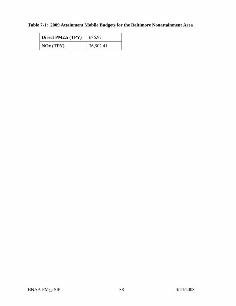
BNAA PM2.5 SIP 3/24/2008 88

able 7-1: 2009 Attainment Mobile Budgets for the Baltimore Nonattainment Area T

Direct PM2.5 (TPY) 686.97

NOx (TPY) 36,502.41

BNAA PM2.5 SIP 3/24/2008 89

8.0 AINMENT AREA PLAN ITMEN

chieving the results shown in this Plan requires a commitment to implement the regulatory easures upon which the plan is based. The States of Maryland is taking action to implement gional measures to reduce emissions of PM2.5 and PM2.5 precursors. Tables 8-1, 8-2, and 8-3

rovide information on the implementation of each measure by Maryland.

ommitments for regulations required by the 40 CFR Part 51 are shown in Table 8-4.

8.1 Schedule of Adopted Control Measures

Table 8-1: Maryland Schedule of Adopted Control Measures


No.

Control Measure Mandate

Regulation

Number

Effective Date

1997 PM2.5 NONATTCOMM TS

Amrep C

Point Source Controls 5.1.1 NOX Phase II Controls Federal

Regulation 26.11.27 & .28 26.11.29 & 30

10/18/99

5.1.1 Regional Transport Requirements / NOx SIP Call

Federal Regulation

26.11.29 26.11.27

5/10/93 No later than Jan.1, 2009

5.1.2 Opacity Regulations Federal Regulation

26.11.01 26.11.06 26.11.07 26.11.08 26.11.09 26.11.10 26.11.12 26.11.18 26.11.20 26.11.25

July 22, 1991 July 18, 2980 January 2, 1980 April 17, 2000 May 28, 1968 May 28, 1968 June 8, 1981 February 10, 1984 November 19, 1983 September 24, 1984

Area Source Controls 5.2.1 Seasonal Open Burning

Restrictions State Regulation 26.11.07 5/22/95

Non-road Source Controls

BNAA PM2.5 SIP 3/24/2008 90

Mandate

Regulation

Effective Date No. Control Measure Number 5.3.1 EP

Engines Rule Federal Regulation

40 CFR parts 90 and 91

12/3/96 A Non-Road Gasoline

5.3.2 EPA Non-Road Diesel Engines Federal 40 CFR Part 9 Model Year 2000-ding on Rule Regulation et al. 2008 depen

engine size 5 ear .3.3 EPA Nonroad Spark Ignition

Marine Engine Rule Federal Regulation

40 CFR Parts 89, 90, 91

1998 Model Y

5

1048, 1051,

2002 .3.4 EPA Large Spark Ignition Engines Rule

Federal Regulation

40 CFR Parts 89, 90, 91, 94,

11/8/

1065, and 1068

5.3.5 Emissions ConLocomotives

6/15/98 trols for Federal Regulation

63 FR 18998

On-road Source Controls 5 High T

MainteFedRegulation

1 1/2.4.1 ech Inspections & nance

eral 1.14.08 /95 & 1/1/2000

5.4.2 tandards e

ederal on

0 CFR part odel Year 1994-p Stds.

Federal Tier I Vehicle Sand new Car EvaporativStandards

FRegulati

486

M1996; Eva1996

5.4.3 National Low Emissions Vehicle Federal 3/22/99 Program Regulation

26.11.20.04

5.4.4 Tier 2 Motor Vehicle EmissionStandards

98 0 Federal Regulation

6

5 FR 66 2/10/200

5.4.5 Heavy-Duty Diesel Engine Rule Federal Regulation

94 63 FR 546 12/22/97

BNAA PM2.5 SIP 3/24/2008 91

8.2 New Source Rev w Permitting Section 173 of the Clean Air Act Amendments require states in PM2.5 nonattainment areas to adopt

r st threshold py for any S iew pollutant, including PM2.5 . Maryland adopt sures, l le 8-4 below.

r m 2.5 ona eas are nincreases of more than 10 tpy PM2.5 or 15 tp 10 any ex ajor facili

tion itting generat o ratio of one to one, and the implementation o hievab s Rate (LAER) for new

odi

Table 8-2: Stationary Source Permitting Re

Baltimore Nonattainment ArState Control Measure Regulation

ber iv

ie

majo ationary source permitting s of 100 ted these mea

regulated Newisted in Tab

ource Rev

Majo odification thresholds in PM n ttainment ar

y PM fromfor net significaisting m

t emissions ty.

Addi al requirements for NSR perm include the

f Lowest Acion or purchasele Emission

f PM2.5 offsets, at a

or m fied units.

visions ea Effect

Nume Date

M NOX Emtationary

COMAR 09.08 Adoption: 0/03

aryland Control of issions for Major SSources

1

8 ity

rdi 1. each PM2.demonstrating that all reasonably available c res, including RACT for stationary

es, en itiously as ave ed. The section mentation rule goes on t otential measures that are reasonably

abl i ity must be C idered collectively, they would advance the attainm ne year or more. As discussed in Section

expected to enable the region to continue to demonstrate compliance with the PM2.5 NAAQS (1997) through the 2009 attainment date. As such, no further action on RACT is warranted.

8.4 Revision of New Source Review (NSR) Regulations In the near future, EPA intends to promulgate further PM2.5 nonattainment requirements, including requirements for precursor emissions, controls and offsets. When these regulations are finalized, state agencies will adopt these changes into their respective state implementation plans.

.3 RACT Applicabil

Acco ng to federal regulation (40 CFR 5 1010) forontrol measu

5 nonattainment area, a SIP revision

sourc necessary to demonstrate attainmof the imple

t as expedo state that p

practicable h been adopt

avail e considering technical and econom c feasibilent date by o

adopted as RA M if, cons

7.2.1, the states determined that there are no additional control measures that could be adopted by January 1, 2008. Further, existing measures, and those planned for implementation by 2009, are

BNAA PM2.5 SIP 3/24/2008 92

t Intentionally Blank This Page Lef

BNAA PM2.5 SIP 3/24/2008 93

9.0 ATTAINMENT PLAN DEMONSTRATION AND WEIGHT OF EVIDENCE

The annual and 24-hour PM2.5 Standard Attainment Demonstration analyzes the potential of the Baltimore Nonattainment Area (NAA) to achieve attainment of the annual and 24-hour PM2.5 standard by April 5, 2010. The attainment demonstration is comprised of the following sections: Modeling Study Overview, Domain and Data Base Issues, Model Performance Evaluation, Attainment Demonstration, Weight of Evidence Demonstration and Procedural Requirements.

9.1 Modeling Study Overview

9.1.1 Background and Objectives On December 17, 2004, the Environmental Protection Agency (EPA) designated areas for the fine particulate matter (PM2.5) National Ambient Air Quality Standards (NAAQS). The standards include an annual standard of 15.0 micrograms per cubic meter (µg/m3) based on the 3-year average of annual mean PM2.5 concentrations, and a 24-hour standard of 65 µg/m3 based on the 3-year average of the 98th percentile of 24-hour concentrations.

The Baltimore, MD Metropolitan Statistical Area (MSA) has been classified as a NAA for PM2.5 with an attainment date of April 5, 2010. Once an area is designated as a NAA, the Clean Air Act requires the submittal of an implementation plan to EPA within three years. State plans are due in April 2008. States may also propose an attainment date extension for up to five years. Those areas for which EPA approves an extension must achieve clean air as soon as possible, but no later than April 5, 2015.

Table 9-1 identifies all jurisdictions that EPA has designated as nonattainment for PM2.5 within the Baltimore NAA.

Table 9-1: Baltimore NAA Designations for 24-Hour and Annual PM2.5 Standards

Jurisdiction Counties Classification Maximum Attainment Date (from 2004)

Maryland

Anne Arundel Baltimore County Baltimore City Carroll Harford Howard

Nonattainment April 5, 2010

Figure 9-1 provides a graphical representation of the Baltimore NAA.

BNAA PM2.5 SIP 3/24/2008 94

he MANE-VU RPO was tasked with the assignment of preparing a PM2.5 modeling platform for ANE-VU states could use to demonstrate compliance with the

(MDE) for preparing this attainment demons or the Baltim

This modeling study is designed to demonstrate attainment of the PM by April 5, 2010. The procedures followed in this lysis are consistent with the EPA’s Guidance on the

FIGURE 9-1: BALTIMORE NAA AND SURROUNDING REGIONS

The State of Maryland is located within the Mid-Atlantic/Northeast Visibility Union (MANE-VU) Regional Planning Organization (RPO)

Tthe MANE-VU region that all MPM2.5 standards. It is the responsibility of the Maryland Department of the Environment

tration f ore NAA.

2.5 standardsmodeling ana

Use of Models and Other Analys ating Attainment of Air Quality Goals for Ozone, es for DemonstrPM2.5, and Regional Haze (EPA- 07-002, Apr454/B- il 2007).

The Baltimore NAA modeling analyses was directed by the MDE with modeling assistance from the niversity of Maryland at College Park (UMD). U

BNAA PM2.5 SIP 3/24/2008 95

9.1.2

he state of Maryland is a member of MANE-VU RPO and along with other member MANE-VU ates, was able to coordinate the modeling analyses performed for the Baltimore NAA with the gional modeling analyses conducted by MANE-VU RPO.

he lead agency for coordinating the running of the CMAQ model and performing the modeling ns for MANE-VU was the New York State Department of Environmental Conservation YSDEC). Modeling centers for MANE-VU included the NYSDEC, University of Maryland at

ollege Park (UMD), the Northeast States for Coordinated Air Use Management (NESCAUM), the ew Jersey Department of Environmental Protection (NJDEP) and the Virginia Department of nvironmental Quality (VADEQ). Even through the NYSDEC was the lead modeling agency for oordinating the running of the CMAQ model for MANE-VU other member states of MANE-VU, ithin the frame-work of MANE-VU, managed the modeling project jointly. All additional odeling for the Baltimore NAA was directed by MDE and performed by UMD under contract with e MDE. All modeling inventories were developed, updated and shared among the regional odeling centers and were provided by MARAMA and MANE-VU.

stallation of the CMAQ model at all participating modeling centers was completed and diagnostic rocedures were run successfully. The CMAQ model was benchmarked against other modeling latforms across the OTR to ensure accurate results.

9.1.3 Conceptual Model

PA recommends that a conceptual description of the area’s PM2.5 problem be developed prior to the

ended that the specific meteorological parameters that

eptual model document, The

Relationship to Regional Modeling Protocols

Tstre

Tru(NCNEcwmthm

Inpp

Einitiation of any air quality modeling study. A “conceptual description” is a qualitative way of characterizing the nature of an area’s nonattainment problem. Within the conceptual description of aparticular modeling exercise, it is recomminfluence air quality be identified and qualitatively ranked in importance. The conceptual model for this study consists of three documents. The first was prepared by NESCAUM for use by the MANE-VU member States. The concNature of the Fine Particle and Regional Haze Air Quality Problems in the MANE-VU Region: A Conceptual Description (NESCAUM, November 2006), is provided in Appendix G-1. This document provides the conceptual description of the fine particle issues in the MANE-VU states, consistent with the EPA’s guidance. The second conceptual description document that is included in Appendix G-1 is The Development of PM2.5 Forecasting Tools for Selected Cities in the MARAMA Region (ICF, September 2004).

he primary objective of the Mid-Atlantic Regional Air Management Association, Inc. (MARAMA) PM2.5 forecasting assistance project was to develop and evaluate statistical-based tools to support PM2.5 forecasting for nine cities in the MARAMA region. The nine cities included Charlotte, North Carolina; Bristol, Roanoke, and Richmond, Virginia; Washington, D.C.; Baltimore, Maryland; Philadelphia, Pennsylvania; Wilmington, Delaware; and Newark/Elizabeth, New Jersey. The study included the analysis of PM2.5 and meteorological data using Classification and Regression Tree (CART) analysis software and the development, testing, and evaluation of interactive forecasting

T

BNAA PM2.5 SIP 3/24/2008 96

tools fo a e course of the project were used, gether with the CART analysis results, to describe the relationships between meteorology and

Appendix G-1 is a Conceptual Model

r each rea. Data and information gathered throughout thtoPM2.5 concentrations and, specifically, the conditions associated with high PM2.5 events in each forecast area. The third conceptual description document that is included inof PM2.5 Concentrations in Maryland (Ryan, May 2007). The purpose of this conceptual model isplace the observations of PM2.5 in the context of climate and weather conditions in order topolicy makers in determining the best implementation plan to reach attainment with the PM2.5 NAAQS.

9.2 Domain and Database Issues

9.2.1 Episode Selection Due to the fact that the attainment demonstration is being conducted using a resource intensivphotochemical grid model, EPA accepts the use of a single, recent “re

to aid

e presentative” year to be used

2.5 are close to the 3-year observed design g sites.

2. The pattern of quarterly mean values is similar to the pattern of quarterly mean

e emission sources, and deled

such

rn, central and southeastern US as well as southeastern Canada.

es

d

for an annual model simulation. Two factors were used in selecting 2002 as the “representative” year:

1. The observed annual mean concentrations of PMvalue at all, or most, monitorin

concentrations averaged over 3 years.

9.2.2 Size of the Modeling Domain In defining the modeling domain, one must consider the location of the local urban area, the downwind extent of the elevated PM2.5 concentrations, the location of largthe availability of meteorological and air quality data. The domain or spatial extent to be moincludes as its core the NAA. Beyond this, the domain includes enough of the surrounding areathat major upwind sources fall within the domain and emissions produced in the nonattainment arearemain within the domain throughout the day.

The boundary of the modeling domain is provided in Appendix G-2. This domain covers the Northeast region including northeaste

9.2.3 Horizontal Grid Size The MANE-VU platform that provides the basic platform for the Baltimore NAA modeling analyshas a coarse grid continental United States (US) domain with a 36-kilometer (km) horizontal grid resolution. The CMAQ domain is nested in the MM5 domain. A larger MM5 domain was selectefor both MM5 simulations to provide a buffer of several grid cells around each boundary of the CMAQ 36-km domain. This was designed to eliminate any errors in the meteorology from boundary effects in the MM5 simulation at the interface of the MM5 model. A 12-km inner domainwas selected to better characterize air quality in the MANE-VU region and surrounding RPO

BNAA PM2.5 SIP 3/24/2008 97

he CMAQ vertical structure is primarily defined by the vertical grid used in the MM5 modeling.

ance

ppendix G-4 contains the vertical layer definitions for the MM5 and CMAQ modeling domains.

The ob d model is to estimate the air quality given a set of eteorological and emissions conditions. When initializing a modeling simulation, the exact

several days prior to the period of interest.

The f polluta ain. An estimate of the quantity of pollutants moving into e ary conditi y boundary conditions for the outer 36-km domain were derived from an annual model run performed by researchers at Harvard University using the

EOS- l. The influence of boundary conditions was ls that

elected for application in the Baltimore NAA modeling analysis. MM5 is a non-hydrostatic, prognostic meteorological model routinely used for

Based on model validation and sensitivity testing, the MM5 configurations provided in Appendix G- were d alyses the including UMD’s detailed performance evaluation

lopment

economic activity as well as the implementation of control measures.

regions. Appendix G-3 contains the horizontal grid definitions for the MM5 and CMAQ modeling domains.

9.2.4 Vertical Resolution TThe MM5 model employed a terrain following coordinate system defined by pressure. The layer averaging scheme adopted for CMAQ is designed to reduce the computational cost of the CMAQ simulations. The effects of layer averaging have a relatively minor effect on the model performmetrics when compared to ambient monitoring data.

A

9.2.5 Initial and Boundary Conditions

jective of a photochemical grimconcentration fields are unknown in every grid cell for the start time. Therefore, typically photochemical grid models are started with clean conditions within the domain and allowed to stabilize before the period of interest is simulated. In practice this is accomplished by starting the model

winds move pollutants into, out of, and within the domain. The model handles the movement onts within the domain and out of the dom

th domain is needed. These are called boundary conditions. To estimate the boundons for the modeling study, three-hourl

G CHEM global chemistry transport modeminimized by using a 17-day ramp-up period, which was sufficient to establish pollutant leveare encountered in the beginning of an air pollution episode.

9.2.6 Meteorological Model Selection and Configuration The Pennsylvania State University/National Center for Atmospheric Research (PSU/NCAR) Mesoscale Meteorological Model (MM5) was s

urban- and regional-scale photochemical regulatory modeling studies.

5o

selecte . Results of various anf the MM5 modeling used in conjunction with the MANE-VU platform are provided in Appendix

G-6.

9.2.7 Emissions Model Selection and Configuration Significant coordination efforts took place between MANE-VU and other RPO’s in the deveof the emissions inventories used in the modeling study. These inventories included a base case (2002), which serves as the “parent” inventory off which all future year inventories (i.e., 2009) are based. The future year inventories include emissions growth due to any projected increase in

BNAA PM2.5 SIP 3/24/2008 98

e Matrix Operator Kernel Emissions (SMOKE) Emissions Processing System was selected for app odeling analysis.

MOKE (Version 2.1) was used for the Baltimore NAA attainment modeling demonstration. 2002

capable considered one of the preferred models for gulatory modeling applications. The model is also recommended by the Guidance on the Use of

The Spars

lication in the Baltimore NAA m

Sbase case and 2009 future base case emissions data files were provided by MANE-VU.

Detailed SMOKE configurations are provided in Appendix G-7.

9.2.8 Air Quality Model Selection and Configuration EPA’s Models-3/Community Multi-scale Air Quality (CMAQ) modeling system was selected for the attainment demonstration primarily because it is a “one-atmosphere” photochemical grid model

of addressing PM2.5 at regional scale and isreModels and Other Analyses for Demonstrating Attainment of Air Quality Goals for Ozone, PM2.5, and Regional Haze (EPA-454/B-07-002, April 2007).

The CMAQ configuration is provided in Appendix G-8.

9.2.9 Quality Assurance All air quality, emissions, and meteorological data were reviewed to ensure completeness, accuracy, and consistency before proceeding with modeling. Any errors, missing data or inconsistencies, were addressed using appropriate methods that are consistent with standard practices. All modeling was benchmarked through the duplication of a set of standard modeling results. Quality Assurance (QA) activities were carried out for the various emissions, meteorological, anphotochemical modeling components of the modeling study. Emissions inventories obtainethe RPOs were examined to check for errors in the emissions estimates. When such errors werediscovered, the problems in the input data files were corrected

d d from

.

The MM t puts were plotted and xamined to ensure accurate representation of the observed data in the model-ready fields, and

ational al and

5 me eorological and CMAQ air quality model inputs and outetemporal and spatial consistency and reasonableness. Both MM5 and CMAQ underwent operand scientific evaluations in order to facilitate the quality assurance review of the meteorologicair quality modeling procedures and are discussed in greater detail throughout this document.

BNAA PM2.5 SIP 3/24/2008 99

9.3 Model Performance Evaluation

e he model’s

lays out the procedures and results of the e i eling process, the emissions and

eteor a e and the desire to keep this report

statistical and graphical evaluations. If the s for the right reasons, then the model can

and their effects on PM2.5.

he res to using modeling to support the

dsheets containing the ssumptions made to compute statistics. Highlights of this evaluation are provided in the following

e issue of model performance goals for PM2.5 is an area of ongoing research and debate. To or air

ve,

eight may be accorded to modeling study results in the decision-making process.

When EPA’s guidance was first developed nearly four (4) years ago, an interim set of fine particulate modeling performance goals were suggested for aggregated mean normalized gross error and mean normalized bias as defined in Table 9-2.

9.3.1 Overview

A critical component of every air quality modeling study is the model performance evaluation wherthe modeled estimates for the base case are compared against observed values to assess taccuracy and provide an indication of its reliability. This section

valuat on. It should be noted that the other parts of the modology, lso undergo an evaluation. It is with this knowledgm

concise, that the air quality model will be the primary focus of this section.

The first step in the modeling process is to verify the model’s performance in terms of its ability to predict PM2.5 and its individual components (i.e., sulfate, nitrate, ammonium, organic carbon, elemental carbon and other constituents) in the right locations and concentrations. To do this, the model predictions for the base year simulation are compared to the ambient data observed in the historical episode. This verification is a combination ofmodel appears to be producing PM2.5 in the right locationbe used as a predictive tool to evaluate various control strategies

T ults of a model performance evaluation were reviewed prior attainment demonstration. The NYSDEC, Division of Air Resources, conducted a performance evaluation of the 2002 base case CMAQ simulation on behalf of the MANE-VU member States. Appendix G-9 and Section 9.5.7 (Weight of Evidence, CMAQ PM2.5 Modeling section) provides comprehensive operational and diagnostic evaluation results, including spreaasections.

9.3.2 Diagnostic and Operational Evaluation Thevaluate model performance, EPA recommends that several statistical metrics be developed fquality modeling. Performance goals refer to targets that a good performing model should achiewhereas performance benchmarks are based on historical model performance measures for the best performing simulations. Performance goals are necessary in order to provide consistency in model applications and expectations across the country and to provide standardization in how much w

BNAA PM2.5 SIP 3/24/2008 100

Table 9 s

Error Normalized Bias

-2. EPA PM2.5 Modeling Performance Goal

Pollutant GrossPM2.5 ~+30 - +50% ~+10% Sulfate ~+30 - +50% ~-20 - -30% Nitrate ~+20 - +70% ~-15 - +50% EC ~+15 - +60% NA OC ~-40 - +50% ~+38%

Because regional-scale PM2.5 modeling is an evolving science, and consideraand performance testing has transpired in the intervening years since these goals were postulated,

ble practical application

d

they are considered as general guidelines.

It may also be possible to adopt levels of model performance goals for bias and gross error as listein Table 9-3 (as developed by the VISTAS RPO) to help evaluate model performance.

Table 9-3. VISTAS RPO PM2.5 Modeling Performance Goals

Fractional Bias Fractional Error Comment

≤±15% ≤35% Ozone model performance goal for which PM2.5 model performance would be considered good.

≤±30% ≤50% A level of model performance that we would hope each PM2.5 species could meet.

≤±60% ≤75% At or above this level of performance indicates fundamental problems with the modeling system.

It does not mean that these performance goals should be generally adopted or

als to use. Rather, the goals are being used to frame and put the PM2.5 model performance into context and to

vity

• Approaching 200% error and ±200% bias when the mean of the observed concentrations are extremely small.

The preceding goals and criteria are not regarded as a pass/fail test, but rather as a basis of inter-comparing model performance across studies, sensitivity tests and models. The OTC model performance evaluation was initially conducted by NYSDEC on the summer ozone season data only. VADEQ has extended the evaluation to include the entire year of 2002

that they are the most appropriate go

facilitate model performance across episodes, species, models and sensititests. As noted in EPA’s PM2.5 modeling guidance, less abundant PM2.5 species should have less stringent performance goals. Accordingly, performance goals that are a continuous function of average observed concentrations such as those proposed by Dr. James Boylan at the Georgia Department of Natural Resources have the following features:

• Asymptotically approaching proposed performance goals or criteria when the mean of theobserved concentrations are greater than 2.5 ug/m3.

BNAA PM2.5 SIP 3/24/2008 101

ded by EPA (Table 9-2) and two adopted y VISTAS RPO (Table 9-3), pertinent to model performance evaluation were computed for FRM

PM2.5 m ind s of C, OM (1.8* blank-corrected OC), soil or crustal l (sum o , F Ti). The statistics were organized into two categories: a) by date For sta s by date, we lculated on a given day for any valid pairs of observe dicted da M and speciation monitors that fall within the OTR modeling

omain plus all Virginia monitors (referred to rom three different

2.5were extracted from CMAQ outputs at the exact

ny v r v d of one calendar year. Again, the full year of 2002 t cJuly 6 and July 9 due to the exceptional even Figu icts the l of the FRM, model evaluation across the OTR+ region. A composite FRM time series across the OTR+ region (264 monitorsThi figure indicates tover-prediction duringis excellent agreement

observations. Four statistical parameters, two recommenb

ass and for ividual specie SO4, NO3, NH4, Emateria f oxides of Ca e, Si, and

and b) by site.

tistic the parameters re cad/pre ta across all FR

d as OTR+). Data collected fmonitoring networks, FRM, STN, and IMPROVE, were used in the statistics. A subset of these “time-based composite monitor" statistics focusing only on Maryland was also generated; see Section 9.5.7 (Weight of Evidence, CMAQ PM Modeling). It is important to note that predicted data used for the model performance evaluation grid cells where monitors are located. This is in contrast to the design value calculations where predictions are based on the average of the surrounding nine grid cells (see Section 9.4 Attainment Demonstration).

or statistics by site, parameters were computed at a given FRM, STN, or IMPROVE monitor for Fa alid pairs of obse

data was used in ved/predicted data ohis “monitor-based

er a perioomposite period" analysis, except for the dates between t caused by the Quebec forest fires.

re 9-2 dep ocation STN and IMPROVE monitor locations used for the

) is provided in Figure 9-3. s hat there is an overall mean bias of approximately 4 µg/m3. There is a general

the winter months and an under prediction during the summer months. There during a mid-August poor air quality episode.

BNAA PM2.5 SIP 3/24/2008 102

FIGURE 9-2. LOCATIONS USED FOR THE MODEL EVALUATION ACROSS THE OTR+REGION: FRM (●, 264), STN (■, 50), AND IMPROVE (▲, 21)

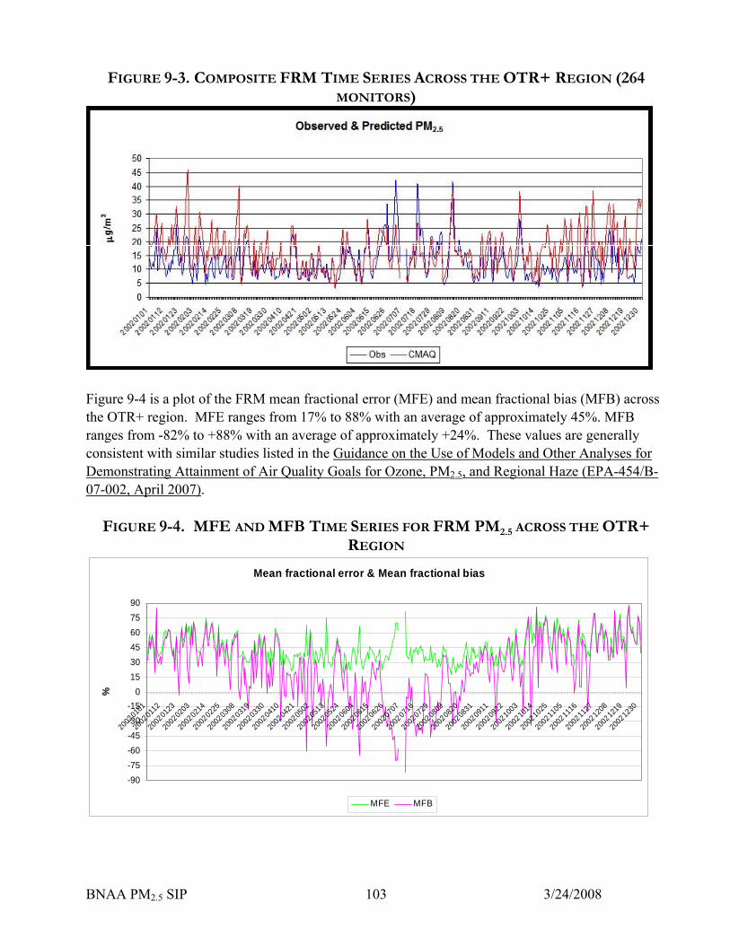
FIGURE 9-3. COMPOSITE FRM TIME SERIES ACROSS THE OTR+ REGION (264 MONITORS)

Figure 9-4 is a plot of the FRM mean fractional error (MFE) and mean fractional bias (MFB) across the OTR+ region. MFE ranges from 17% to 88% with an average of approximately 45%. MFB ranges from -82% to +88% with an average of approximately +24%. These values are generally consistent with similar studies listed in the Guidance on the Use of Models and Other Analyses for Demonstrating Attainment of Air Quality Goals for Ozone, PM2.5, and Regional Haze (EPA-454/B-07-002, April 2007).

FIGURE 9-4. MFE AND MFB TIME SERIES FOR FRM PM2.5 ACROSS THE OTR+ REGION

Mean fractional error & Mean fractional bias

-90-75-60-45-30-15

0153045607590

2002

0101

2002

0112

2002

0123

2002

0203

2002

0214

2002

0225

2002

0308

2002

0319

2002

0330

2002

0410

2002

0421

2002

0502

2002

0513

2002

0524

2002

0604

2002

0615

2002

0626

2002

0707

2002

0718

2002

0729

2002

0809

2002

0820

2002

0831

2002

0911

2002

0922

2002

1003

2002

1014

2002

1025

2002

1105

2002

1116

2002

1127

2002

1208

2002

1219

2002

1230

%

MFE MFB

BNAA PM2.5 SIP 3/24/2008 103

BNAA PM2.5 SIP 3/24/2008 104

An es are the best a model can be expected to ach criteria” curves are considered acceptable for model performance. 258 of 264 sites satisfy the “criteria” restriction on an annual average basis.

FIGURE 9-5. MFE BUGLE PLOT FOR FRM PM ACROSS OTR+ REGION

MFE bugle plot for FRM PM2.5 across OTR+ region is provided in Figure 9-5. “Goal” curvieve while the “

2.5

FRM PM2.5

020406080

100120140160180200

0 3 6 9 12 15 18 21

Observed, µg/m3

MFE

, %

FRM Goal Criteria

MFE bugle plots were also generated for SO4, NO3, and NH4, EC, OM, and soil/crustal across OTRregion and are provided in Figures 9-6 through 9-11. As can be seen from the results, theperformance for indiv

+

idual species is generally consistent with the criteria necessary for acceptable odel performance.

FIGURE 9-6. MFE BUGLE P O ACROSS OTR+ REGION

m

LOT FOR S 4

Sulfate

020406080

100120140160180200

0 1 2 3 4 5 6 7 8 9 10

Observed, µg/m3

MFE

, %

STN IMPROVE Goal Criteria

FIGURE 9-7. MFE BUGLE PLOT FOR NO3 ACROSS OTR+ REGION

Nitrate

020406080

10012014016012

0 0.4 0.8 1.2 1.6 2 2.4 2.8 3.2 3.6 4

Observed, µg/m3

MFE

, %

8000


FIGURE 9-8. MFE BUGLE PLOT FOR NH ACROSS OTR+ REGION 4

Ammonium

180200

020406080

100120140160

0 0.4 0.8 1.2 1.6 2 2.4 2.8 3.2 3.6 4

Observed, µg/m3

MFE

, %


BNAA PM2.5 SIP 3/24/2008 105

FIGURE 9-9. MFE BUGLE PLOT FOR EC ACROSS OTR+ REGION

Elemental Carbon

020406080

100120140160180200

0 0.3 0.6 0.9 1.2 1.5 1.8 2.1 2.4

Observed, µg/m3

MFE

, %


FIGURE 9-10. MFE BUGLE PLOT FOR OM ACROSS OTR+ REGION

Organic Mass

020406080

100120140160180200

0 1 2 3 4 5 6 7 8 9 10

Observed, µg/m3

MFE

, %


BNAA PM2.5 SIP 3/24/2008 106

BNAA PM2.5 SIP 3/24/2008 107

FIGUR GION E 9-11. MFE BUGLE PLOT FOR SOIL/CRUSTAL ACROSS OTR+ RE

Soil/crustal

020406080

100120140160180200

0 0.1 0.2 0.3 0.4 0.5 0.6 0.7 0.8 0.9 1

Observed, µg/m3

MFE

, %


Concentrat are easily met. Concentration-dependent performance criteria for nitrate, organic mass, and soil/crustal material are met at nearly all IMPROVE sites and most STN sites. The following is a list of several PM2.5 statistics for the OTC domain that have also been provided in Appendix G-9.

1. Statistical evaluation of daily average PM2.5 mass from FRM sites across the OTR+ domain. Statistics are computed by date and by site (across the OTR+). [Figure 9-3, Figure 9-4 (by date), Figure 9-5 (by site).]

2. Statistical evaluation of daily average PM2.5, SO4, NO3, NH4, EC, OM, and crustal/soil

mass at EPA STN sites. Statistics are computed by date and by site (across the OTR+). [Figure 9-5 to Figure 9-11 (by site).]

3. Statistical evaluation of daily average PM2.5, SO4, NO3, EC, OM, and crustal/soil mass at

IMPROVE sites. Statistics are computed by date and by site (across the OTR+). [Figure 9-5 to Figure 9-11 (by site).]

here was insufficient data to warrant a separate statistical evaluation of individual species focusing n the Baltimore NAA monitors. Only two speciation monitors (both STN) are located in the

Baltimore NAA.

ion-dependent performance goals for sulfate, ammonium, and elemental carbon

To

BNAA PM2.5 SIP 3/24/2008 108

CMAQ was employed to simulate PM2.5 for the calendar year 2002. A review of PM2.5 and its individual species was conducted for the study domain. The CMAQ model performance for surface PM2.5 is good with acceptable bias and error. Several observations can be made with respect to model performance, including the following:

1. Organic matter (OM) is comprised of primary and secondary components. Approximately 80-90% of CMAQ calculated OM consists of primary OM. Observed OM has a distinct maximum during the summer when secondary formation is highest; CMAQ exhibits substantial under-prediction of secondary organic aerosol (SOA) formation.

2. CMAQ captures seasonal variation in SO4 well. 3. CMAQ appears to overestimate primary PM2.5 components (EC, soil, primary OM),

especially during colder months. 4. CMAQ appears to underestimate secondary OM during the summer.

easonal biases in the CMAQ calculated PM2.5 component concentrations are not of great regulatory

concern since attainment tests are based on the application of relative response factors to observed

g to erent manner between regions.

xamination of the statistical metrics by sub-region confirms the absence of significant performance

ing consistently across the full OTC domain. This confidence in the modeling ults allows for the modeling system to be used to support the State Implementation Plan (SIP) to

meet th

9.4

As previou s been classified as a NAA area for PM2.5 with an attainm nt date of April 5, 2010. The PM2.5 NAAQS includes an annual standard of 15.0 µg/m3 based oµg/m3 base

his sectio onstrate attainment of the NAAQS in

9.3.3 Summary of Model Performance

S

concentrations. In summary, the regional and local model performance is acceptable for PM2.5. While there are some differences between the spatial data between sub-regions, there is nothinsuggest a tendency for the model to respond in a systematically diffEproblems arising in one area but not in another, building confidence that the CMAQ modeling system is operatres

e 24-hour and annual PM2.5 NAAQS.

Attainment Demonstration

9.4.1 Overview

sly mentioned, the Baltimore MSA haen the 3-year average of annual mean PM2.5 concentrations, and a 24-hour standard of 65

d on the 3-year average of the 98th percentile of 24-hour concentrations.

n summarizes the procedures that were used to demTthe State Implementation Plan (SIP) package. As described in EPA’s Guidance on the Use of Models and Other Analyses for Demonstrating Attainment of Air Quality Goals for Ozone, PM2.5, and Regional Haze (EPA-454/B-07-002, April 2007), an attainment demonstration consists of (a) nalyses which estimate whether selected emissions reductions will result in ambient concentrations

that meet the NAAQS, and (b) an identified set of control measures which will result in the required emissions reductions. The necessary emission reductions for both of these attainment demonstration components may be determined by relying on results obtained with air quality models.

a

BNAA PM2.5 SIP 3/24/2008 109

EPA gu inment test to the air quality modeling results to etermine if the PM NAAQS will be met. Additional technical or corroboratory analyses may also

tion support a demonstration of attainment of

e NAAQS.

The purposimplement AAQS for PM by the attainment year of 2009. The modeling is applied in a relative sense, similar to the 8-hour t test is more complicated and reflects the fac a separate re lated for each of the PM2.5 components. Since the attainm referred to as the

peciated Modeled Attainment Test (SMAT). The following sections outline the process to

e

, with

For the SMAT process, a mean PM DVB is determined, as well as component specific DVB for each qu calculation of baseline design values needed for

e PM attainment test.

ean PM2.5 Baseline Design Values

d ated

g the composition that

.

idance recommends applying a modeled attad 2.5

be used as part of a “supplemental analysis” or a more stringent “weight of evidence” determinato supplement the modeled attainment test and to furtherth

The modeled attainment test is described in further detail in the following portions of this section, and the additional corroborative analyses are presented in Section 9.5.

9.4.2 Modeled Attainment Test

e of a modeling assessment is to determine if control strategies currently being ed (“on the books”) and proposed control strategies will lead to attainment of the N

2.5 ozone attainment test. However, the PM2.5 attainment that PM2.5 is a mixture. In the test, ambient PM2.5 is divided into major components, with

lative response factor (RRF) calcuent test is calculated on a per species basis, the attainment test for PM2.5 is

Sdetermine if 2009 projections of PM2.5 will meet the NAAQS from regional modeling, as suggested in EPA’s guidance. Determine Baseline Design Values The first step in any attainment test process is to determine the baseline design value (DVB). EPA guidance recommends using a DVB that is the average of the three design value periods that straddlthe baseline inventory year (i.e., the average of the 2000-2002, 2001-2003, and 2002-2004 design value periods for a 2002 baseline inventory year). This works out to a 5-year weighted averagethe baseline year having the heaviest weight (i.e., {[2000] + 2*[2001] + 3*[2002] + 2*[2003] + [2004]}/9).

2.5arter. The following section will detail the

th 2.5

MTo begin the SMAT process, a mean PM2.5 DVB is calculated on a quarterly basis for each Federal Reference Method (FRM) monitor in the PM2.5 nonattainment areas. Concentrations are calculatebased on calendar quarters (Q1: January - March; Q2: April - June; etc.) as the NAAQS is calculfor a calendar year, and the quarters need to fit evenly within a year. Also, calculatinattainment test on a quarterly basis allows states to examine the differences in PM2.5 occur during the different seasons. Speciated Baseline Conditions The monitored attainment test for PM2.5 utilizes both PM2.5 and individual PM2.5 component speciesA separate RRF is calculated for each PM2.5 species. In order to perform the recommended modeled attainment test, States should divide observed mass concentrations of PM2.5 into 7 components (plus passive mass):

BNAA PM2.5 SIP 3/24/2008 110

ssociated with particle bound water (PBW)

he sec quarterly mean PM2.5 DVBs (as calculated in the Section

s entrations (and percent contributions to PM2.5 mass), which may be different than the

cal cons

ater, inferred carbonaceous material balance approach” or SANDWICH W e mass is adjusted to account for volatilization

from mass balance ([OCMmb] = PM2.5FRM:{[EC] + [SO4] + al material] + [passive mass]}).

sts four measures that can be taken to resolve the lack of speciated data:

1. Mass associated with sulfates (SO4) 2. Mass associated with nitrates (NO3) 3. Mass associated with ammonium (NH4) 4. Mass associated with organic carbon (OC) 5. Mass associated with elemental carbon (EC) 6. Mass a7. Mass associated with “other” primary inorganic particulate matter (Crustal) 8. And passively collected mass or the mass of the blank filter

TM

ond part of the process is to use the ean PM2.5 Baseline Design Values) with speciated data to calculate the quarterly mean

concentrations of these 7 components at the FRM sites. This need to speciate the FRM data presents two issues:

1. FRM measurements and speciated PM2.5 measurements do not always measure the same mass.

2. Not all FRM monitoring sites have co-located STN speciation monitors.

The following sections will explain how these issues were overcome to produce the speciated valuesneeded for this attainment demonstration. SANDWICH As EPA guidance states, recent data analyses have noted that the FRM monitors do not measure the same components and do not retain all of the PM2.5 that is measured by routine speciation samplers and therefore cannot be directly compared to speciation measurements from the Speciation Trends Network (STN). By design, the FRM mass measurement does not retain all ammonium nitrate and other semi-volatile materials (negative sampling artifacts) and includes particle bound water (PBW) associated with sulfates, nitrates and other hygroscopic species (positive sampling artifacts). Thiresults in concambient levels of some PM2.5 chemi tituents. To resolve the differences between FRM and STN total mass, EPA recommends using the “sulfate, adjusted nitrate, derived wapproach. ith the SANDWICH approach, nitratbased on hourly meteorological parameters. Subsequently, quarterly average nitrate, sulfate, elemental carbon, and crustal mass can be calculated, as well as the Degree of Neutralization (DON)of sulfates. Quarterly average NH4 can then be calculated from adjusted the adjusted nitrate mass, sulfate mass, and DON of sulfate. Next the mass of PBW can be calculated from the previously obtained DON, sulfate, nitrate, and ammonium values. Finally, organic carbon is calculated by taking the difference between the total PM2.5 mass as measured at the FRM monitor, and the calculated component mass (i.e., OC[NO3] + [NH4] + [water] + [crust Speciated Profiles While the SANDWICH method reconciles the differences between FRM and STN, a lingering issue is that not all FRM monitoring sites have co-located STN monitors to provide speciated data. EPA guidance sugge

BNAA PM2.5 SIP 3/24/2008 111

speciated monitor ferent time period)

a spatial field using ambient speciation data tial fields, and gridded modeling outputs to

Of on techniques to esti tion data (numbers 3 and 4 bove). To assist in this task, the EPA is currently developing a software tool called “Modeled

onstration

ue to the MATS tools being unavailable at the time of this analysis, it was decided to investigate the Baltim sex site was chosen due to the extensive speciated database and the rep ional composition of PM2.5 at Essex should contain a larger contribution from organic carbon and elemental carbon and

is approach makes the calculation more conservative. The bserved contribution of Ammonium, Elemental Carbon, Nitrate, Organic Carbon, Sulfate, Other

2.5 at both the Essex and Fort Meade monitoring

this study was performed using the EPA commended method for “nearby” grid cells for a 12-kilometer horizontal grid resolution, with a

h

d

predicted peak. If a State were to tention only to the cell containing a monitor, it might underestimate the RRF

ns.

1. Use of concurrent data from a near by2. Use of representative data (from a dif3. Use of interpolation techniques to create 4. Use of interpolation techniques to create spa

adjust the species concentrations

the four methodologies, the EPA recommends using one of the spatial interpolatimate species concentrations at FRM sites that do not have specia

aAttainment Test Software” (or MATS) that will perform the spatial analysis of described options number 3 and 4. However, the MATS tool was unavailable at the time this modeling demwas being prepared. When the MATS tool is available it will be used as recommended by EPA. D

use of speciated data from either the Fort Meade or Essex monitoring sites located within the ore NAA. The Es

resentativness of the data (i.e., urban). When averaged over a season, the fract

a smaller contribution from sulfate, nitrate, and ammonium than a more rural site. Since the largest reductions are projected to be in sulfate, thoPrimary PM2.5, and PBW by percentage of total PMsites are provided in Section 9.5.7 (Weight of Evidence, CMAQ PM2.5 Modeling). Appendix G-10 contains data needed to calculate 24-hour and annual design values. After evaluating both the Fort Meade and Essex speciated data it was decided that the Essex data would be used, as it would give the most conservative estimate of future year design values. Relative Response Factor Calculations The calculation of relative response factors (RRFs) forre3x3 grid cell array for 12-km resolution modeling. The RRF used in the modeled attainment test is computed by taking the ratio of the mean of the predictions in the future to the mean predictions witbaseline emissions, over all relevant days.

For the 24-hour and annual PM2.5 NAAQS, the spatially averaged value of the nearby predictions (mean value of the grid cell array) was used. Each component-specific RRF was used in the modeleattainment test by taking the ratio of the mean of the spatially averaged daily predictions in the future to the mean of the spatially averaged daily predictions with current emissions.

The basis for this approach is as follows:

1. Consequence of a control strategy may be “migration” of a confine its at(i.e., overestimate the effects of a control strategy).

2. Uncertainty in the formulation of the model and the model inputs is consistent with recognizing some leeway in the precision of the predicted location of concentratio

BNAA PM2.5 SIP 3/24/2008 112

is to start in the southwest corner of onsidering several cells “near” a

m.

4. The area does not exhibit strong spatial concentration gradients of observed primary PM2.5.

3. Standard practice in defining a gridded modeling domain the domain, and determine grid cell location from there. Cmonitor rather than the single cell containing the monitor diminishes the likelihood of inappropriate results, which may occur from the geometry of the superimposed grid syste

Annual SMAT Results

Table 9-4 presents the results of the annual SMAT results for the Baltimore NAA. The SMAT results demonstrate that the projected average annual arithmetic mean PM2.5 concentration calculatedat each FRM monitor attains the annual PM2.5 NAAQS. Specifically, all future design value (DVF) alculations are less than15.0 µg/m3. c

It is important to note that an attempt was made to calculate a DVF at each of the FRM monitors. EPA guidance is somewhat unclear as to what constitutes a valid number of quarters necessary to calculate a DVF. Special attention should be paid to this when reviewing the results in Table 9-4 Monitors with 19 or 20 valid quarters are generally considered to have a more reliable DVF than those with incomplete data.

Table 9-4 Annual SMAT Results for Baltimore NAA 2009 Beyond-On-The-Way Control Measures

2000-2004 DVB 2009AIRS ID Site Name County State Q1 Q2 Q3 Q4 #Q DVF24- 0 15.32 9.42 19 10.3 003-0014 Davidsonville Anne Arundel MD 9.03 13.224- 11.2 003-0019 Ft. Meade Anne Arundel MD 10.39 14.04 16.38 10.15 20 24- 13.2 003-1003 Glen Burnie Anne Arundel MD 13.91 15.08 17.11 13.43 20 24- 12.2 003-2002 Rivera Beach Anne Arundel MD 12.46 14.39 16.08 11.99 20 24- MD 12.79 14.07 16.21 11.70 20 12.2 002-1007 Padonia Baltimore 24- 13.0 005-3001 Essex Baltimore MD 14.13 14.37 16.52 13.11 20

24- 12.4 510-0006 NE Police Station Baltimore (Baltimore City) MD 13.09 14.33 16.23 11.83 20

24- 12.9 510-0007 NW Police Station Baltimore (Baltimore City) MD 13.71 15.18 17.11 12.17 20

24- y) 510-0008 SE Police Station Baltimore (Baltimore Cit MD 14.29 16.68 17.29 13.72 16 13.8

24- 13.8 510-0035 FMC-Fairfield Baltimore (Baltimore City) MD 15.47 15.27 17.35 14.06 20

24-510-0040 Old Town Baltimore (Baltimore City) MD 16.14 15.88 18.00 14.55 20 14.4

24- 20 13.2 510-0049 Westport Baltimore (Baltimore City) MD 13.26 15.88 17.02 13.20

24- MD 11.41 13.31 14.82 10.53 20 11.2 025-1001 Edgewood Harford 24-Table 9results etic mean PM2.5 concentration calculated at e e (DVF) cal

Hour SMAT Results -5 presents the results of the 24-hour SMAT results for the Baltimore NAA. The SMAT demonstrate that the projected average annual arithm

ach FRM monitor attains the 24-hour PM2.5 NAAQS. Specifically, all future design valuculations are well below 65 µg/m3.

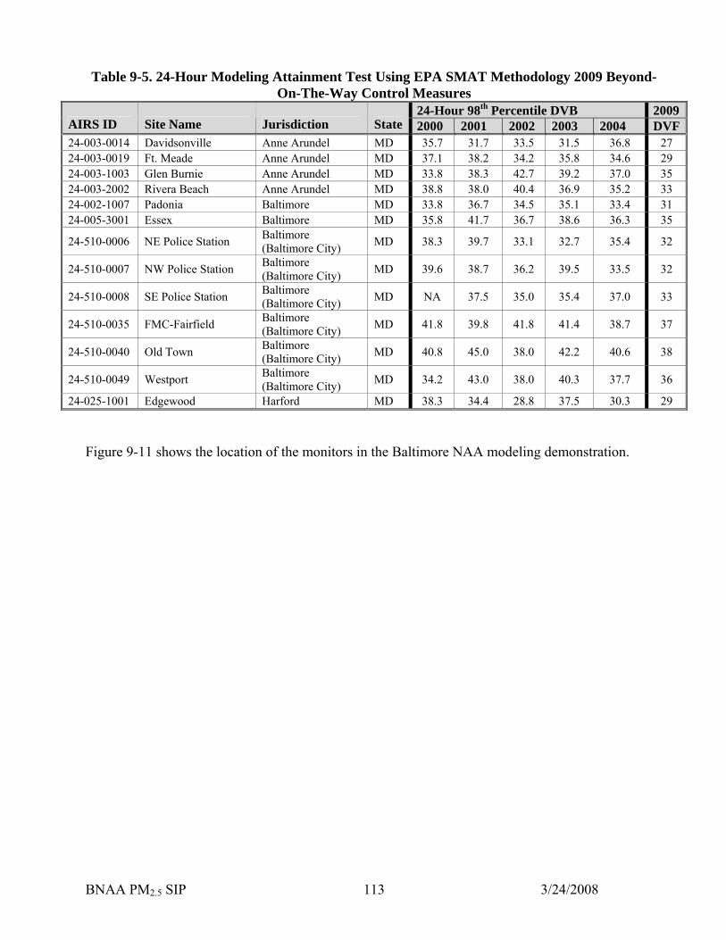
BNAA PM2.5 SIP 3/24/2008 113

Table 9-5. 24-Hour Modeling Attainment Test Using EPA SMAT Methodology 2009 Beyond-On-The-Way Control Measures

24-Hour 98th Percentile DVB 2009AIRS ID Site Name Jurisdiction State 2000 2001 2002 2003 2004 DVF24-003-0014 Davidsonville Anne Arundel MD 35.7 31.7 33.5 31.5 36.8 27 24-003- 9 29 001 Ft. Meade Anne Arundel MD 37.1 38.2 34.2 35.8 34.6 24- Anne Arundel MD 33.8 38.3 42.7 39.2 37.0 35 003-1003 Glen Burnie 24- Anne Arundel MD 38.8 38.0 40.4 36.9 35.2 33 003-2002 Rivera Beach 24-0 31 02-1007 Padonia Baltimore MD 33.8 36.7 34.5 35.1 33.4 24-005-3001 Essex Baltimore MD 35.8 41.7 36.7 38.6 36.3 35

24- 510-0006 NE Police Station Baltimore (Baltimore City) MD 38.3 39.7 33.1 32.7 35.4 32

24- re ore City) MD 39.6 38.7 36.2 39.5 33.5 32 510-0007 NW Police Station Baltimo

(Baltim

24- 33 510-0008 SE Police Station Baltimore (Baltimore City) MD NA 37.5 35.0 35.4 37.0

24- 37 510-0035 FMC-Fairfield Baltimore (Baltimore City) MD 41.8 39.8 41.8 41.4 38.7

24- (Baltimore City) 38 510-0040 Old Town Baltimore MD 40.8 45.0 38.0 42.2 40.6

24- ort Baltimore MD 34.2 43.0 38.0 40.3 37.7 36 510-0049 Westp (Baltimore City) 24-025-1001 Edgewood 37.5 30.3 29 Harford MD 38.3 34.4 28.8

9-1 location onitors in lt e N mo g d nstr . Figure 1 shows the of the m the Ba imor AA delin emo ation

BNAA PM2.5 SIP 3/24/2008 114

M FIGURE 9-11. BALTIMORE NONATTAINMENT AREA PM2.5 MONITORS USED IN THE

ODELING DEMONSTRATION


PM2.5 Monitor


PM2.5 Monitor

Baltimore Nonattainment AreaBaltimore Nonattainment Area

PM2.5 MonitorPM2.5 Monitor

9.4.3 Unmonitored Area Analysis The modeled attainment test does not address future air quality at locations where there is not a PM2.5 monitor nearby. To guard against the possibility that air quality levels could exceed the standard in areas with limited monitoring, EPA suggests that additional review is necessary, particularly in nonattainment areas where the PM2.5 monitoring network just meets or minimally exceeds the size of the network required to report data to Air Quality System (AQS). This review is intended to ensure that a control strategy leads to reductions in PM2.5 and its constituent pollutants at other locations that could have baseline (and future) design values exceeding the NAAQS were a monitor deployed there. The test is called an “unmonitored area analysis”. The purpose of the analysis is to use a combination of model output and ambient data to identify areas that might exceed the NAAQS if monitors were located there. It is important to note that the Baltimore NAA currently operates a network of 10 PM2.5 monitors. Several of these monitors were established as State and Local Air Monitoring Stations (SLAMS). These SLAMS monitors were selected based on specific monitoring objectives (background concentration, area of highest concentration, high population, source impact, transport, and rural impact) as required by EPA and siting scales (micro, middle, neighborhood, urban, and regional) established by EPA.

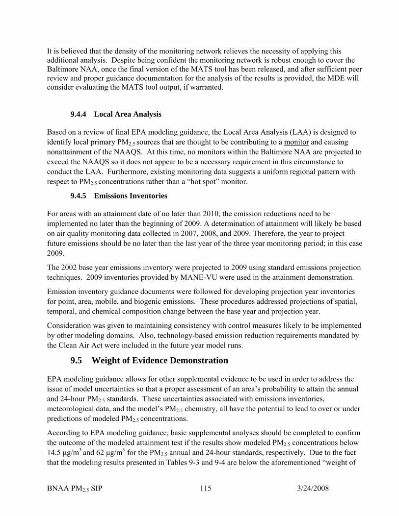
BNAA PM2.5 SIP 3/24/2008 115

It is believed that the density of cessity of applying this additional analysis. Despite being confident the monitoring network is robust enough to cover the Baltimore NAA, once the final version of the MATS tool has been released, and after sufficient peer review and proper guidance documentation for the analysis of the results is provided, the MDE will consider evaluating the MATS tool output, if warranted.

9.4.4 Local Area Analysis Based on a review of final EPA modeling guidance, the Local Area Analysis (LAA) is designed to identify local primary PM2.5 sources that are thought to be contributing to a monitor

the monitoring network relieves the ne

and causing nonattainment of the NAAQS. At this time, no monitors within the Baltimore NAA are projected to exceed the NAAQS so it does not appear to be a necessary requirement in this circumstance to conduct the LAA. Furthermore, existing monitoring data suggests a uniform regional pattern with respect to PM2.5 concentrations rather than a “hot spot” monitor.

9.4.5 Emissions Inventories For areas with an attainment date of no later than 2010, the emission reductions need to be implemented no later than the beginning of 2009. A determination of attainment will likely be based on air quality monitoring data collected in 2007, 2008, and 2009. Therefore, the year to project future emissions should be no later than the last year of the three year monitoring period; in this case 2009.

The 2002 base year emissions inventory were projected to 2009 using standard emissions projection techniques. 2009 inventories provided by MANE-VU were used in the attainment demonstration.

mission inventory guidance documents were followed for developing projection year inventories for poi , s. These procedures addressed projections of spatial,

mporal, and chemical composition change between the base year and projection year.

ted d by

2.5 emistry, all have the potential to lead to over or under

below

t

Ent, area mobile, and biogenic emission

te

Consideration was given to maintaining consistency with control measures likely to be implemenby other modeling domains. Also, technology-based emission reduction requirements mandatethe Clean Air Act were included in the future year model runs.

9.5 Weight of Evidence Demonstration EPA modeling guidance allows for other supplemental evidence to be used in order to address theissue of model uncertainties so that a proper assessment of an area’s probability to attain the annual and 24-hour PM2.5 standards. These uncertainties associated with emissions inventories,

eteorological data, and the model’s PM chmpredictions of modeled PM2.5 concentrations.

According to EPA modeling guidance, basic supplemental analyses should be completed to confirmthe outcome of the modeled attainment test if the results show modeled PM2.5 concentrations 14.5 µg/m3 and 62 µg/m3 for the PM2.5 annual and 24-hour standards, respectively. Due to the facthat the modeling results presented in Tables 9-3 and 9-4 are below the aforementioned “weight of

BNAA PM2.5 SIP 3/24/2008 116

vidence” thresholds established by EPA, a limited supplemental analysis was deemed necessary to

supporting evidence presented in Appendix

-11, the conclusion will be reached that Maryland is pursing an effective and comprehensive PM2.5 trategy, which will lead to attainment of the annual and 24-hour PM2.5 NAAQS.

2.5 Values

2.5 NAAQS of 65 µg/m3 and that the esign value since the period 2000-2002, which has

esupport the 2009 attainment demonstration

This section will primarily be based on the work completed by the UMD, which examines the state of the science of aerosols over the Mid-Atlantic region, focuses on trends and both measurement andmodeling uncertainties of PM2.5. After examining all the Gs

9.5.1 Trend in PM Design Figures 9-12 and 9-13 show trends in annual and daily PM2.5 design values, respectively. It is clearfrom Figure 9-12 that there is a downward trend in annual PM2.5 design value since the period 2000-2002. During the period 2003-2005, the design value rose slightly but once again continued its downward trend during 2004-2006 time period. Figure 9-13 shows the Baltimore NAA is well below the 24-hour PM

re is also a downward trend in the dcontinued through the period 2004-2006. A downward trend in both annual and 24-hour PM2.5 design values indicate that the control measures implemented during this period have been providing PM2.5 reduction benefits. With more controls anticipated in coming years, this trend is expected to continue.

BNAA PM2.5 SIP 3/24/2008 117

ROM 2002-2006. 28 FIGURE 9-12. ANNUAL PM2.5 DESIGN VALUES FOR BALTIMORE NONATTAINMENT

AREA F

Baltimore Nonattainment AreaAnnual PM2.5 Design Value (2002-2006)

17.417.417.5

18

)

16.316.6

2000-2002 2001-2003 2002-2004 2003-2005 2004-2006

16.0

15

15.5

16

16.5

Des

ign

Val

ue (u

g/m

3)

17

13.5

14

14.5Annual PM2.5 Design Value (ug/m3)Annual PM2.5 Standard (15 ug/m3)

FIGURE 9-13. 24-HOUR PM2.5 DESIGN VALUE FOR BALTIMORE NONATTAINMENT

AREA FROM 2002-2006. 29

Baltimore Nonattainment Area24-Hour PM2.5 Design Value (2001-2006)

42.041.0 41.0

39.0

43.0

30

35

40

45

50

55

60

65

70

2000-2002 2001-2003 2002-2004 2003-2005 2004-2006

Des

ign

Val

ue (u

g/m

3) )

24-Hour PM2.5 Design Value (ug/m3)24-Hour PM2.5 Standard (65 ug/m3)

28 Data from EPA Air Trends: Design Values Website at http://www.epa.gov/airtrends/values.html 29 Data from EPA Air Trends: Design Values Website at http://www.epa.gov/airtrends/values.html

BNAA PM2.5 SIP 3/24/2008 118

The observations indicate that the chemical composition, spatial distribution, and seasonal cycle of PM2.5 are reasonably well understood. This information can be used to determine if the right aerosols and PM2.5 precursors are being controlled in the right places and at the right times. Measurements of PM2.5 show, in the context of abatement strategy, uniformity in composition and concentration across the Mid-Atlantic region. Sulfate peaks in the summer and nitrate peaks in the winter, but regionally during the course of a year, the makeup and levels of aerosols are reasonably consistent with the bulk of the mass identified. In round numbers (to the nearest 5%), and in decreasing importance, an analysis of the IMPROVE data identifies the main contributors to PM2.5 as ammonium sulfate (50%), organic matter (25%), ammonium nitrate (10%), mineral dust (5%), and BC (5%). The EPA/State CSN data show ammonium sulfate (40%), organic matter (40%), ammonium nitrate (15%), mineral dust (5%), and BC (5%). The winter peak in nitrate indicates that NOx controls should be utilized year-round. The small fraction of total PM2.5 mass attributable to mineral dust suggests that control of local emissions of crustal elements from construction activities for example, can have only a minor impact on the annual PM2.5 concentrations. Maryland and the surrounding States have been working through various control programs to lower year-round regional emissions of SO2, NOx, primary OC (including BC), and VOC’s, and this approach appears to be targeting the right species in the appropriate spatial and temporal scales. Appendix G-10, Section I, examines the typical values and variability in chemical composition, spatial distribution, and seasonal cycle of PM2.5 its major chemical constituents.

9.5.3 Review of Literatur The scientific literature on PM2.5, especially as it relates to PM2.5 in Maryland indicates that the PM2.5 problem is regional in nature. With this in mind some of the sources hundreds of km’s away are providing much of the problem of the aerosols in Maryland. Sulfate dominates the regional picture, though local PM2.5 and precursor sources are also important. The PM2.5 problem in Maryland is part of a broader regional problem, thus the focus on regional controls, especially regional SO2 controls, in the Maryland SIP is a step in the right direction. It should also be mentioned that local and regional VOC controls as well as NOx controls should also have some impact on PM2.5. In all, direct observations, modeling, source apportionment, back trajectory and clustering techniques have been used to create a coherent picture of the PM2.5 problem in the East, especially as it applies to Maryland. Sulfate emerges as the dominant contributor and is responsible for a large share of the PM2.5 problem and an even larger share of the visibility problem, while OC and nitrate are smaller, but still significant contributors to the PM2.5 problem. Reductions in SO2 and NOx emissions have been conclusively linked to reductions in sulfate and nitrate. The literature review in Appendix G-11, Section II, discusses experimental campaigns in Maryland first, then regional campaigns and lastly data analysis efforts. Based on this literature review it can be concluded that controlling SO2 (especially on the regional scale), VOC’s, and NOx should lead to continued significant reductions in PM2.5 over Maryland.

9.5.2 The Composition of PM2.5

e on PM2.5

BNAA PM2.5 SIP 3/24/2008 119

-Atlantic Region

st rly,

M2.5

f the

9.5.4 PM2.5 Trends Over the Mid Monitors over the Mid-Atlantic region show a decrease in PM2.5 concentrations ranging from 0.117 to 0.360 micrograms per-cubic meter per-year (µg m-3 yr-1), with a mean trend of ~0.25 µg m-3 yr-1. The trends are statistically significant at each site (p < 0.05) and at all sites together (p < 0.01). At all locations investigated as part of this study, sulfate was the PM2.5 species that contributed the moto the decrease in PM2.5, and was responsible for ~50% of the PM2.5 decrease on average. Similaorganic carbon accounts for ~25% of the decrease and ammonium ~15%. Nitrate, dust and elemental carbon contribute to the trend in a smaller way. While definitively quantifying the regional signal of PM2.5 is a complex problem, the homogeneity in the trend of PM2.5 and Pspecies suggests all monitors in this study share a common regional “load” of PM2.5. Comparison ofthe urban and rural monitors suggests the regional load may account for roughly 60%-75% ototal observed PM2.5 (see http://www.epa.gov/air/airtrends/aqtrnd03/pdfs/2_chemspecofpm25.pdf). Inspection of seasonal cycles suggests the regional contribution may increase during parts of the summer season, but the seasonality of the species distribution in fact has changed little over the pasten years. Recently implemented regional control strategies, which target sulfur, nitrogen and emissions, should continue the current trend of further reducing PM2.5 concentrations on the worst air quality days in Maryland. While there is site to site and year to year variability in PM2.5 readthis consistent decrease in PM2.5 concentrations suggests that Maryland and the surrounding areas are targeting the appropriate PM2.5 species at the appropriate

t VOC

ings,

locations.

In App f PM2.5 over the Mid-Atlantic region are assessed in rder to describe the current state and future projections regarding air quality over Maryland.

2.5 episodes in Maryland have vealed that in many instances SO2 from electric utilities and VOCs from mobile sources are

ppendix G-11, Section IV will examine emissions reductions in Maryland and the MANE-VU

endix G-11, Section III temporal trends o

o

9.5.5 PM2.5 Composition As it Relates to Effectiveness of Controls Several source apportionment and highly time resolved analyses of PMreresponsible for the sulfate and the organic portion of PM2.5. Other studies have shown that in Maryland and the Northeast region, sulfate is the largest contributor to PM2.5, and that sulfate andnitrate respond positively to reductions in SO2 and NOx emissions. An analysis of the 2002 NEI andthe 2009 projected emissions inventory for Maryland and MANE-VU shows that the emissions controls that will go into place in and surrounding Maryland are geared towards reducing SO2, NOx, and VOC emissions from electric utility and mobile sources. Given the historical trend of decreasing emissions of SO2, NOx, and VOC’s coupled with decreases in sulfate, nitrate, organic matter, and PM2.5, it can be expected that PM2.5 in Maryland will decline substantially in the future. Aregion to determine the effectiveness of reducing PM2.5 and to determine if emissions reductions projected for 2009 target the correct PM2.5 constituent and source.

BNAA PM2.5 SIP 3/24/2008 120

tion Sites

2.5 and nal

n

everal monitoring sites in and around Maryland.

ance

5 udget restimation of cond es in biogenic

-3 t

e 2.5

9.5.6 Monitoring Data From Surface-Based Specia The concentrations of PM2.5 and its speciated components have been monitored at several sites in and around Maryland for several years. The overall accuracy of the instruments used in these analyses has been assessed. Daily measurement of PM2.5 (based on a side-by-side comparison of FRM and CSN filter-based 24-hr average) or its major constituents can be taken with 95% confidence limit within about 30% of the actual value. Precision is substantially better than absolute accuracy, and long-term averages are accurate to better than 20%. Chemically speciated PMassociated trace gases (including NH3, HNO3, CO, SO2, and NOy) reflect both local and regiosources. Day-to-day and seasonal variations in the PM2.5 chemical composition reflect changes iboth the weather and in the contribution from various sources. Appendix G-11, Section V examines the origins, properties, and statistical distributions of PM2.5 at s

9.5.7 CMAQ PM2.5 Modeling The performance of CMAQ was examined and found to be acceptable for use in Maryland’s PM2.5 attainment demonstration. In particular, for Maryland, the largest changes in any PM2.5 species are projected to occur in sulfate, and this is the one species where CMAQ’s performance is at its best. Most other species show relatively more modest improvements in fine particle concentrations.

MAQ’s performance is poorest for soil/crustal material and organic matter. The poor performCfor soil/crustal material is only a minor concern since soil/crustal material only comprises 3-6% of PM2.5 in the Mid-Atlantic region. The underestimation of summertime organic matter oncentrations by CMAQ is of more concern since organic matter is an important part of the PM2.c

b at some Mid-Atlantic locations. Much of the bias is likely due to an undeary organic aerosols, most of which have a biogenic source. Since changse

emissions are expected to be small over the next decade, CMAQ-calculated relative response factors for organic matter is not crucial. In addition, following EPA guidance, the impact of this bias is minimized by normalizing model predicted changes in organic matter by observed PM2.5 partitioning. Therefore CMAQ’s PM2.5 modeling performance is acceptable for this modeling demonstration. Biases in CMAQ and the Beyond OTB/OTW inventory used in the model are such that the calculated future design values are somewhat higher than they would likely be in reality. These calculations are therefore conservative with regard to Maryland’s PM2.5 attainment status. PM2.5 concentrations were calculated for all Maryland monitors. Based on these calculations, Maryland will be in attainment for all applicable PM2.5 NAAQS by 2009. The highest Maryland monitor is calculated to continue to be the Old Town monitor in downtown Baltimore. This monitor

predicted to have a 2009 design value range of 14.0-14.4 µg m-3, a range that is just below the islower threshold of the weight of evidence range (14.5 – 15.5 µg m ). In the future, it appears thaMaryland will continue to make steady progress in reducing PM2.5 concentrations after the 2009 attainment deadline. Should the annual PM2.5 standard be tightened in the future, Maryland will b

ell positioned for continued attainment of the PM NAAQS. w

BNAA PM2.5 SIP 3/24/2008 121

Appen 1 tified in the CMAQ odel. It also examines how well CMAQ simulates PM2.5 concentrations over the Mid-Atlantic

ocum s developed in this study are available for

,

t participant l

he .

dix G-1 , Section VI discusses and quantifies all biases that are idenmregion.

9.6 Summary and Conclusions of Attainment Demonstration The results from the modeling as well as the weight of evidence supplemental analyses present overwhelming evidence that the Baltimore NAA will attain the 24-hour and annual PM2.5 NAAQS by April 5, 2010. Based on air quality measurements and future predicted air quality modeling results, the projected design values are below the NAAQS attainment criteria of 15.0 µg/m3 for annual PM2.5 and 65 µg/m3 for 24-hour PM2.5.

9.7 Procedural Requirements

9.7.1 Reporting D ents, technical memorandums, and data basedistribution as appropriate. This report contains the essential methods and results of the conceptual model, episode selection, modeling protocol, base case model development and performance testingfuture year and control strategy modeling, quality assurance, supplemental analyses, and calculationof PM2.5 attainment via EPA’s methodology.

9.7.2 Data Archival and Transfer of Modeling Files All relevant data sets, model codes, scripts, and related software required by any projecnecessary to corroborate the study findings (e.g., performance evaluations, control strategy runs) wilbe provided in an electronic format approved by the MANE-VU RPO within the framework of tMANE-VU RPO. The MANE-VU RPO has archived all modeling data relevant to this projectTransfer of data may be facilitated through the combination of a project website and the transfer of large databases via overnight mail. Database transfers will be accomplished using an ftp protocol forsmaller datasets, and the use of IDE and Firewire disk drives for larger data sets.

BNAA PM2.5 SIP 3/24/2008 122


BNAA PM2.5 SIP 3/24/2008 123

10.0 CONTIN The General Preamble and EPA guidance defines the requirements for identification of contingency measures for attainment demonstrations. For attainment demonstrations, contingency measures may reduce emissions of NOX, SO2, or PM2.5 direct. Contingency measures are required for each milestone year. Air quality plans must include sufficient contingency measures to account for one year of reductions needed to attain.

10.1 Contingency Measures for the Attainment Demonstration

10.1.1 Background

EPA requires the Baltimore region to include a contingency plan containing adopted measures that qualify as contingency measures for the Attainment Demonstration. This section fulfills the requirement for the Attainment contingency.

10.1.2 Required Reductions The contingency measures for the attainment demonstration must total one year of reductions needed to attain. The inventory is calculated as described in Sections 3 and 4. Table 10-1 shows the calculation of the necessary reductions.

Table 10-1: Contingency Requirement for PM and PM Precursors

PM and PM Precursor Emissions 2002-2009 (tons per year)

GENCY PLAN

PM Precursor 2002 2009 2002-2009

Contingency Requirement Calculation

(2002-2009)/7

NOX 130,925.57 83,107.03 47,818.54 6,831.22

SO2 108,192.96 122,261.62 (14,068.66) None*

PM2.5 Direct 14,434.04 14,932.68 (498.65) None* * = No contingency measures required because emissions increase between 2002 and 2009.

Contingency reductions must occur on a timetable that is directly related to the Attainment SIP schedule. States have no more than one year after notification by EPA of an attainment failure to achieve the contingency plan reductions. For a potential attainment failure, notification would be received in 2010, therefore the contingency reductions must be achieved no later than 2011. According to EPA guidance, emission reductions from different PM precursors can be used to meet the required contingency target. EPA recommended a method to assess equivalent reductions for different precursors. The recommended approach is to review existing data and sensitivity studies performed as part of photochemical modeling to estimate the relative impact of reductions in

BNAA PM2.5 SIP 3/24/2008 124

g an equivalency ratio on relative reduction factors rate X for each ton of SO2

X

an are well in excess of these tios and therefore should be an appropriate backstop for improving air quality should the

monito .

tingency Measures

SO2. ingency reductions, therefore meeting the contingency

easure requirement calculated in Table 10-1. The contingency measures for the metropolitan Baltimo cess of the equivalency ratios described in Section 10.1.2 nd therefore should be an appropriate backstop for improving air quality should the monitoring

Table 10-2: Contingency Measures for 2008 PM Attainment

Ref. No. (tons/year) (tons/year)

different precursors on PM concentrations. Basins gene d by the CMAQ modeling, results in a ratio of 1.1 to 1.4 tons of NOa

(see Appendix F). Using these relative reduction factor generated equivalency ratios, the conservative SO2 contingency requirement is 6,210.2 tons. Using sensitivity analyses created by VISTAS and Georgia Tech (see Appendix F), equivalency ratios range from 3.3 to 3.6 tons of NO for each ton of SO2. Using the VISTAS/Georgia Tech generated equivalency ratios, the conservative SO2 contingency requirement is 2,070.1 tons. As discussed in Section 10.1.3, the

opolitan Baltimore attainment plcontingency measures for the metrra

ring network not demonstrate compliance with the 1997 PM2.5 NAAQS in 2009

10.1.3 Identified Con Table 10-2 lists the contingency measure identified by the State of Maryland for the Attainment Demonstration. This measure delivers a total benefit of more than 82,678 tons per year (tpy) The reduction is greater than the required contm

re attainment plan are well in exanetwork not demonstrate compliance with the 1997 PM2.5 NAAQS in 2009.

2.5(Tons per Year)

Contingency Measure SO2 NOX

5.2.2 Tier 2 Motor Vehicle Emission Standards 0

5.2.1 Healthy Air Act SO2 Reductions 82,678.5 0

TOTAL REDUCTIONS In accordan h EPA’s courag pleme ontinge res to guard agains a e to eithe ilestone or plement the contingency sures iden le 10 to the icated i ers 5 and 8. EPA early ation o easures is as follows:

ce wit guidance en ing early im ntation of c ncy measut f ilur mea

r meet a mtified in Tab

attain, the Maryland w-2 according

ill im timetable ind n Chapt

’s guidance on implement f control m

The EPA encourages the early implementation of required control measures and of contingency measures as a means of guarding against failures to meet a milestone or to attain. Any implemented measures (that are not needed for the rate-of-progress requirements or for the attainment requirements) would need to be backfilled only to the extent they are used to meet a milestone.

The reductions from the designated contingency measures are surplus vis-à-vis the Attainment demonstration contained in this SIP. They will not be used to meet that milestone requirement. As a result, the states will not be required to backfill any contingency measures that they choose to implement in advance of the requirement.

BNAA PM2.5 SIP 3/24/2008 125

ppendix B – Projection Year Methodologies

ppendix C – Reasonably Available Control Measures (RACM) Analysis

ppendix F – Contingency Synopsis of the ASIP Sensitivity Study

Appendix G – Attainment Modeling Appendix G-1: Appendix G-2: Modeling DomAppendix G-3: Horizontal Grid Definitions for MM5 and CMAQ Modeling Domain Appendix G-4: Ver r MM5 and C Model main Appendix G-5: MMApp - Appendix G-7: Configuration Appendix G-8: Appendix G-9: nce Appendix G-10: n Design Value Cal ulations Appendix G-11: Weight of Evidence Report

APPENDICES Appendix A –Base Year Emission Inventory

Appendix A-1: Base Year Emission Inventory Methodologies Appendix A-2: Point Source Base Year Inventory Appendix A-3: Quasi-Point Source Base Year Inventory Appendix A-4: Area Source Base Year Inventory Appendix A-5: Mobile Source Base Year Inventory Appendix A-6: Nonroad Source Base Year Inventory

A

AAppendix C-1: List of Potential RACM Control Measures & Analysis Appendix C-2: BMC Reduction Measures List & Analysis

Appendix D –Mobile Budget Documentation Appendix E – OTC MOU A

Conceptual Model ain Boundary

tical Layer Definitions fo5 Model Configuration

MAQ ing Do

endix G 6: MM5 Model Performance EvaluationSMOKE Processing Description and CMAQ Configuration CMAQ Model PerformaAdditional Information o c

baltimore nonattainment area pm state … · 1.3 sip process ... appendix f – contingency...

Documents