background subtraction for open heavy avour studies in proton-proton ... · pdf filebackground...

Background subtraction for open heavy flavour studies

in proton-proton collisions at √ s = 7 TeV with the

ALICE Muon Spectrometer

Fatiha Lehas

To cite this version:

Fatiha Lehas. Background subtraction for open heavy flavour studies in proton-proton collisionsat

√s = 7 TeV with the ALICE Muon Spectrometer. Physics [physics]. 2014. <dumas-

01240663>

HAL Id: dumas-01240663

https://dumas.ccsd.cnrs.fr/dumas-01240663

Submitted on 9 Dec 2015

HAL is a multi-disciplinary open accessarchive for the deposit and dissemination of sci-entific research documents, whether they are pub-lished or not. The documents may come fromteaching and research institutions in France orabroad, or from public or private research centers.

L’archive ouverte pluridisciplinaire HAL, estdestinee au depot et a la diffusion de documentsscientifiques de niveau recherche, publies ou non,emanant des etablissements d’enseignement et derecherche francais ou etrangers, des laboratoirespublics ou prives.

https://hal.archives-ouvertes.fr

https://dumas.ccsd.cnrs.fr/dumas-01240663

Distributed under a Creative Commons Attribution - NonCommercial - NoDerivatives 4.0International License

http://creativecommons.org/licenses/by-nc-nd/4.0/



UFR sciences et

technologies

Laboratoire dephysique

corpusculaire

Blaise Pascal University

Master Report

Background subtraction for open heavyflavour studies in proton-protoncollisions at

√s = 7 TeV with the

ALICE Muon Spectrometer

Author:

Fatiha LEHAS

Supervisor:

Dr. Lizardo Valencia Palomo

June 2014

ii

Abstract

With ultrarelativistic high energy heavy-ion collisions it is possible to reproduce, during

a short time, the Quark Gluon Plasma : a dense and hot matter that existed in the early

universe some microseconds after the big bang. Among the experiments at the LHC,

ALICE is the only one that was designed and built to study heavy ion collisions. The

muon spectrometer of the ALICE experiment studies open heavy flavours, quarkonium

and low mass resonance through their semileptonic and leptonic decay into single muons

and dimuons. The present report focuses on the study of open heavy flavours in proton-

proton collisions as they can be used to test perturbative QCD calculations but also

as a reference in Pb-Pb collision measurements. The first chapter introduces basic

concepts of heavy ion collisions and open heavy flavour production in proton proton

collisions. The second chapter contains a description of the ALICE experiment and the

muon spectrometer. Chapter three describes the method used to extract the single muon

distribution coming from open heavy flavours and the associated systematic uncertainties

to the background subtraction. Finally, chapter four is a summary of the most important

results obtained.

iii

Resume

Avec les collisions des ions lourds a des energies ultrarelativistes il est possible de re-

produire, pendant un court lap de temps, une plasma de quark et de gluon (QGP) :

une matiere dense et chaude qui existait dans l’univers primordial quelques microsec-

ondes apres le big bang. Parmi les experiences au LHC, ALICE est la seule qui a ete

concu et construite pour etudier les collisions d’ions lourds. Le spectrometre a muons

de l’experience ALICE etudie les saveurs lourdes ouvertes, quarkonium et les resonances

a faible masse a travers leurs desintegration leptonique et semileptonique en muons et

dimuons. Le rapport actuel se concentre sur l’etude des saveurs lourdes ouvertes dans

les collisions proton-proton comme ils peuvent etre utilises pour tester les calculs de la

QCD perturbative mais aussi comme une reference dans les collisions Pb-Pb. Le premier

chapitre introduit les concepts basiques des collisions des ions lourdes et la production

des saveurs lourdes ouvertes dans les collisions protons-protons. Le deuxieme chapitre

contient une description de l’experience ALICE et le spectrometre a muons. Le chapitre

trois decrit la methode utilisee pour extraire la distribution du muon provenant des

saveurs lourdes ouvertes et les uncertitudes systematiques associees a la soustraction

du bruit de fonds. Finalement, le chapitre quatre est un resume des resultats les plus

importants obtenus.

Acknowledgements

I thank Allah the Almighty for giving me the will and courage to complete this modest

master’s report. I extend my thanks to my project advisor, Doctor.Lizardo Valencia

Palomo, for his invaluable advice and availability throughout the preparation of this

work. I am thankful to the ALICE group in the LPC at Clermont-Ferrand for their

collaboration. I want to thank all my friends who helped me from far and near to

complete this work. I conclude by thanking my parents that I have always trusted.

iv

Contents

Abstract ii

Resume iii

Acknowledgements iv

Contents v

List of Figures vii

List of Tables ix

1 Introduction 1

1.1 Preleminaries . . . . . . . . . . . . . . . . . . . . . . . . . . . . . . . . . . 1

1.2 QCD phase transition diagram . . . . . . . . . . . . . . . . . . . . . . . . 2

1.3 Nucleus-nucleus collisions . . . . . . . . . . . . . . . . . . . . . . . . . . . 3

1.3.1 Space-time evolution . . . . . . . . . . . . . . . . . . . . . . . . . . 4

1.3.2 The importance of open heavy flavours . . . . . . . . . . . . . . . . 5

1.3.3 Factorization theorem . . . . . . . . . . . . . . . . . . . . . . . . . 6

1.3.4 Open heavy flavour in pp collision . . . . . . . . . . . . . . . . . . 7

2 ALICE Experiment 9

2.1 The Large Hadron Collider . . . . . . . . . . . . . . . . . . . . . . . . . . 9

2.2 The ALICE Experiment . . . . . . . . . . . . . . . . . . . . . . . . . . . . 11

2.2.1 Central barrel . . . . . . . . . . . . . . . . . . . . . . . . . . . . . . 11

2.2.2 Forward Muon spectrometer . . . . . . . . . . . . . . . . . . . . . 14

2.2.3 Absorbers . . . . . . . . . . . . . . . . . . . . . . . . . . . . . . . . 15

2.2.4 Tracking system . . . . . . . . . . . . . . . . . . . . . . . . . . . . 15

2.2.5 Trigger system . . . . . . . . . . . . . . . . . . . . . . . . . . . . . 16

2.2.6 Dipole magnet . . . . . . . . . . . . . . . . . . . . . . . . . . . . . 16

3 Background subtraction 17

3.1 Realistic simulations . . . . . . . . . . . . . . . . . . . . . . . . . . . . . . 17

3.2 pT -shape of the background . . . . . . . . . . . . . . . . . . . . . . . . . . 19

3.3 Background Normalization . . . . . . . . . . . . . . . . . . . . . . . . . . . 22

3.4 Results . . . . . . . . . . . . . . . . . . . . . . . . . . . . . . . . . . . . . . 24

3.5 Systematic uncertainties . . . . . . . . . . . . . . . . . . . . . . . . . . . . 25

v

Contents vi

4 Conclusion 29

A π/K Dominant Primary particles 31

B Scaling factors 35

Bibliography 37

List of Figures

1.1 QCD phase diagram. . . . . . . . . . . . . . . . . . . . . . . . . . . . . . . 2

1.2 The time evolution of the collision of two nuclei. . . . . . . . . . . . . . . 4

2.1 Layout of the acceleration chain at CERN . . . . . . . . . . . . . . . . . . 10

2.2 The ALICE experiment . . . . . . . . . . . . . . . . . . . . . . . . . . . . 12

2.3 The forward Muon spectrometer layout of main components. An absorberto filter the background, a set of tracking chambers before, inside and afterthe magnet and a set of trigger chambers. . . . . . . . . . . . . . . . . . . 14

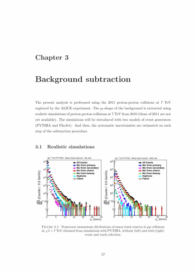
3.1 Transverse momentum ditributions of muon track sources in pp collisionsat

√s = 7 TeV obtained from simulations with PYTHIA, without (left)

and with (right) event and track selection. . . . . . . . . . . . . . . . . . . 17

3.2 The production mechanisms for different muon track sources. . . . . . . . 18

3.3 Fit and extrapolation of the primary muons pt-spectrum in the 5η binsusing PYTHIA (left) and PhoJet (right). . . . . . . . . . . . . . . . . . . 20

3.4 Comparison between the pT -shape of primary muons in the total accepat-nce −4.0 < η < −2.5 (red line) and the sum from the fit in the 5 pseudo-rapidity bins (green lines). Left panel : PYTHIA. Right panel : PhoJet. . 21

3.5 Estimated ratio of primaries (scaled) to inclusive muons for real dataand Monte Carlo simulations (left) and comparison between the inclusivespectrums of real data and Monte Carlo simulations (right) in the 5 η bins. 23

3.6 The same as figure.3.5 in −4.0 < η < −2.5. . . . . . . . . . . . . . . . . . 24

3.7 Left panel : yield of muons before background subtraction and the meanyield after the background subtraction from PYTHIA and PhoJet as afunction of pT in −4.0 < η < −2.5. Right panel : yield of muons beforeand after background subtraction as a function of η and for 2 < pT < 20GeV. . . . . . . . . . . . . . . . . . . . . . . . . . . . . . . . . . . . . . . . 25

3.8 Estimated systematic uncertainties for σmodel (left) and σnorm (right) inthe 5 η bins. . . . . . . . . . . . . . . . . . . . . . . . . . . . . . . . . . . . 26

3.9 Estimated systematic uncertainties for σmodel (left) and σnorm (right) inthe total acceptance. . . . . . . . . . . . . . . . . . . . . . . . . . . . . . . 27

vii

List of Tables

3.1 Estimated systematic uncertainties for σmodel and σnorm. . . . . . . . . . . 28

A.1 Produced primary particles according to PYTHIA . . . . . . . . . . . . . 31

A.2 Produced open charm particles according to PYTHIA . . . . . . . . . . . 32

A.3 Produced open beauty particles according to PYTHIA . . . . . . . . . . . 32

A.4 Produced primary particles according to PhoJet . . . . . . . . . . . . . . 32

A.5 Produced open charm particles according to PhoJet . . . . . . . . . . . . 32

A.6 Produced open beauty particles according to PhoJet . . . . . . . . . . . . 33

B.1 Scaling factors (rounded) used to scale the background to the real data . 35

B.2 Scaling factors used for background subtraction and to compute σnorm. . 36

ix

Chapter 1

Introduction

In this chapter, we present the importance of heavy ion collisions studies and how it is

related to the Quark-Gluon-Plasma. Production of open heavy flavour in proton-proton

collision and their role to verify pertubative QCD calculations are also presented.

1.1 Preleminaries

The heavy flavour discovery took place in 1974 when the J/ψ particle was first registered.

The particle was identified as a bound state of the quark charm and its anti-quark. It

was not only the discovery of a new particle but also the discovery of a fourth quark

after the u, d and s. Other heavy particles, which one of the constituants was a c

quark, are called open charm like Λ+c , D

0 and D+ that were discovered in 1975 and 1976

repectively. In 1977, the Υ particle, a bound state of beauty (bottom) quark and its

anti-quark, was discovered. Five years later, the open beauty particles B0 and B+ were

discovered [1].

The production of heavy flavours can only occur in the initial hard scatterings of the

collision because of their large mass. It is then possible to use perturbative QCD (pQCD)

calculations to compute heavy flavours production cross-sections. Besides that, the

charm and beauty hadrons became a powerful tool to investigate the properties of the

dense and hot medium that is created in ultra-relativistic heavy ion collisions.

At the present LHC energies, 2.75 TeV for Pb-Pb collisions, charm and beauty produc-

tion is abundant: the cross-section increases by about a factor 10 for charm and 100

for beauty with respect to RHIC top energy. The large yields of c and b quarks allow

detailed studies on the heavy flavour energy loss as well as on the possible charm and

1

Chapter 1. Introduction 2

Figure 1.1: QCD phase diagram.

beauty thermalization in the QCD medium. On this respect, in order to constrain the-

oretical models, it is of crucial importance to have an experimental apparatus capable

of measuring separately open charm and beauty hadrons [2].

1.2 QCD phase transition diagram

Lattice QCD calculations predict that at sufficiently high energy density and tempera-

ture, ordinary nuclear matter undergoes a phase transition from a confined to a decon-

fined state where quarks and gluons are asymptotically free. This new state of matter

is called Quark-Gluon-Plasma (QGP) (figure.1.1) and is thought to have existed in the

early universe some microseconds after the big bang. The only way to recreate the

QGP in the laboratory is by reproducing the same conditions of high energy density

and temperature with high energy heavy-ion collisions.

The basic idea in heavy ion collisions, is that a large amount of energy is deposited in a

small volume [3, 4].

A considerable attention has been paid to whether a critical point exists on the phase

diagram of strongly interacting matter. One very important issue is whether the critical

point can be found in experiments that involve colliding heavy nuclei.


The QCD phase diagram has two axes: the temperature T and the density (chemical

potential for quark number) µ. The chemical potential is directly related to the net quark

density (i.e., the number of quark minus number of antiquarks). We can extract the main

features of the QCD phase diagram by first setting either µ or T to zero. Imagine the

early universe when its temperature was much higher than the critical temperature of

deconfinement, which is about 200 MeV. The early universe contained practically the

same number of quarks and antiquarks, (so µ = 0.) At such high temperatures, we

have a plasma of quarks and gluons, and the interaction between these particles is weak,

thanks to asymptotic freedom.

As the universe cools down, the interaction becomes stronger and two things happen.

The first is confinement: quarks and gluons are combined into hadrons (bound states

of three quarks, or one quark and one antiquark). There does not have to be a phase

transition associated with confinement alone (in a later state in the evolution of the

universe, electrons and protons would recombine into hydrogen without going through

phase transition).

The second phenomenon is spontaneous breaking of chiral symmetry. Under chiral

symmetry, different types of left handed quarks (with spin pointing against the direction

of motion) transform into each other (right to left handed and left to right handed), while

independently right-handed quarks (spin pointing to the same direction as momentum)

transform into each other. Chiral symmetry would be an exact symmetry of QCD if

quarks were massless. In the real world u and d quark (i.e., the two types of quarks that

combine to form neutrons and protons) are not massless, but very light, so the chiral

symmetry is not exact.

Let us now stay on the other axis, at zero temperature, by increasing the quark chemical

potential (see figure.1.1), one first jumps from vacuum to nuclear matter. This jump is

definitely a first-order phase transition and what happens at higher chemical potential is

less clear. It is rather well established that if u and d are the only relevant quarks, then

at extremely high densities chiral symmetry should be restored. Therefore, there must

be another chiral phase transition on the µ axis. In contrast to the finite-temperature

chiral phase transition, there is no reliable information about the location and the nature

of this chiral phase transition [4].

1.3 Nucleus-nucleus collisions

The principle purpose of ultrarelativistic nucleus-nucleus collisions is to obtain informa-

tion on the QCD phase diagram. Indeed, it was argued that the quark-hadron phase


Figure 1.2: The time evolution of the collision of two nuclei.

transition drives the equilibration dynamically, at least for the SPS energies and above

[5].

During the process of multiple nucleon-nucleon collision occurring in a nucleus-nucleus

collisions, the nucleons lose a fraction of their energy. At low energies, nucleons are

stopped in the collision region, giving birth to a state with high chemical potential µB.

At very high energies, the nucleons can still have enough momentum to continue with

their trajectory and move far away from the interaction point. The energy lost is then

deposited in the collision region creating a high energy nuclear matter with small µB.

1.3.1 Space-time evolution

If the energy of the collision is high enough, the QGP can be created. If the plasma

reaches the thermal equilibrium, its evolution will follow the laws of thermodynamics. As

the system expands, its temperature also drops down, giving place to hadronization. The

space-time evolution of a high energy heavy-ion collision is the following (see figure.1.2)

[3, 6].

• Heavy quarks, jets and direct photons are created in the initial hard scattering (t

≈ 0 fm/c). These processes are well described by pQCD.

• Multiple scattering among partons and produced particles lead to a rapid increase

of entropy which could result in thermalization (t ≈ 1-2 fm/c).

• The system reaches the deconfined phase (t ≈ 10-15 fm/c).


• The expanding system cools down and below the critical temperature quarks and

gluons become confined into hadrons (t ≈ 20 fm/c).

• Inelastic processes are reduced until the relative abundance of hadrons is fixed

(chemical freeze-out). Finally, all the interactions cease and created hadrons

stream out (kinetic freeze-out).

The standard scenario for a high energy nucleus-nucleus collision involves several stages

(see figure.1.2). At extremely short times scales take place the very hard processes that

account for the hard particles in the final state. The bulk of this particle production

takes place slightly later (t ∼ 0.2 fm/c). Eventually, this deconfined matter reaches a

state of local thermal equilibrium, and can be described by hydrodynamics. Because it

is in expansion, it cools down and reaches the critical temperature where hadrons are

formed again. At a later stage, the density becomes too low to have an interaction rate

high enough to sustain equilibrium, and the system freezes out.

Experimentally, one is trying to infer properties of the early and intermediate stages of

these collisions from the measured hadrons in the final state [3].

1.3.2 The importance of open heavy flavours

With the new scale of energy in Pb-Pb collision at the LHC, ten times higher than that

reached by Relativitic Heavy Ion Collider (RHIC), a deconfined state of quarks and

gluons is expected to be formed (µB ≈ 0). Since the lifetime of that medium (≈ 0.5 - 1

fm/c) is larger than the production time scale of the heavy flavours (1/mQ), then heavy

quarks play a crucial role to study the properties and provide information on that new

state of matter [7].

Heavy quarks can be used as probes to understand the in-medium partonic energy loss

in the dense QCD matter created in a central heavy-ion collision.

The nuclear modification factor RAA is an experimental observable defined by the equa-

tion.1.1. It quantifies the deviation of particle production in nucleus-nucleus collisions

with respect to proton collisions binary scaling.

RAA =1

< Ncoll >× d2NAA/dptdη

d2Npp/dptdη(1.1)

where d2NAA/dptdη is the number of measured particles per unit of transverse momen-

tum and pseudorapidity in A-A collisions, d2Npp/dptdη the number of the same kind of

particles measured in pp collisios and < Ncoll > the mean number of nucleon-nucleon


collisions. If RAA = 1, then there is no difference between the production in nucleus-

nucleus and in pp collisions. But if RAA 6= 1, then it might be an indication of medium

induced effects [2, 8].

Measurements of the heavy-flavour production in proton-proton collisions are necessary

to obtain the nuclear modification factor. Moreover, studies of charm and beauty pro-

duction in pp collisions at the LHC allows to test pQCD models in a new energy domain

[9].

1.3.3 Factorization theorem

The theoretical predictions in nucleon-nucleon collisions are based on the factorization

theorem in the framework of the pQCD calculations to compute the cross section for

heavy flavours.

According to that theorem, the process of nucleon-nucleon collisions could be explained

in the following steps:

• In the initial stage, two partons i and j are extracted from the two colliding nucleon

each of momentum xi/j with probablities given by the parton distribution function

fi/j(xi/j , µ2F ) such that i/j is parton species (q,q,g) and µF is the factorization

scale.

• In the following stage and during hard scatterings between the two partons, heavy

flavours are produced with virtuality Q ∼ x1x2SNN where SNN is the center of

mass energy. In that stage, when mQ > ΛQCD, the elementary cross section is

related to the interaction at high Q2 and can be computed in pQCD in terms of

αks . αs is the strong coupling constant and k indicates the perturbative order.

• After the formation of the heavy quark, it will interact with other partons and

hadronize into open heavy flavour hadrons with a probability DHQ

Q (z) where z is

the momentum fraction pHQ/pQ.

So according to those three steps, the hadronic production of open heavy flavours is

characterized by three quantities: fi/j(x, µF ) partonic distribution function (PDFs),

partonic cross section dσij→Q(Q)n/dpt and the fragmentation function DHQ

Q (z). The

large mass of open heavy flavour hadrons makes those three parameters different in

properties than light hadrons.

One of the advantages of heavy flavours is that they allow to access small Bjorken-

x range, in particular at high center-of-mass collision energy and/or large (pseudo)-

rapidity. At LHC energies, in pp collisions at√sNN = 7 TeV, one can access Bjorken-x


values down to x ∼ 4.10−4 (1.10−3) for charm (beauty) quarks in the mid-rapidity region.

Thanks to higher energies reached at the LHC than at RHIC, heavy quarks allow to

probe the low Bjorken-x region dominated by gluons at the LHC. When the rapidity

increases, unprecedented low Bjorken-x values can be investigated. In the acceptance of

the forward muon spectrometer of ALICE, −4.0 < η < −2.5, the accessible Bjorken-x

range is down to 10−6.

In the partonic cross section, each order of αs is accompanied by logarithmic terms as a

coefficient ∼ (αslnτ)n (τ is an arbitrary order parameter) when the perturbative series

end up. A Fix Order (FO, with a given power n) cross section is used to different orders

of logarithmic terms.

For n = 0, one obtains the Leading Order (LO) cross section with O(αs)(or the Born

term) and n = 1 (O(α2s)) corresponds to the Next-to-Leading Order (NLO) cross section.

With a given fixed order n and using k = n one obtains the Leading Logarithm (LL)

terms. The Next-to-Leading Logarithm (NLL) terms are obtained by adding to the LL

terms the k = n− 1 terms. For reasonable consideration FO and NLL calculations were

matched as the so called FONLL (Fixed-Order Next-to-Leading Logarithm) formalism.

1.3.4 Open heavy flavour in pp collision

The production cross section of b and c quarks can be predicted using pQCD due to their

large masses (mQ > ΛQCD). The predictions by the different models do not give the

complete description of non perturbative phenomena that contribute in heavy flavour

production.

Heavy flavours studies were performed by different experiments at Tevatron and RHIC.

D meson production cross section was measured at√s = 1.96 TeV and compared to

FONLL calculations. The measured differential cross sections was found to be higher

than the theoretical predictions by about 100% at low pt and 50% at high pt, but they

are compatible with the calculations within uncertainty bands.

In the case of beauty quark, the measurements were different. The production cross

section were better described by theory. The J/ψ pt distribution from the inclusive

decays B → J/ψ +X was measured by the CDF collaboration. It was found that the

data points lie well within the uncertainty band and they are in very good agreement

with the central FONLL prediction [1, 10–12].

Chapter 2

ALICE Experiment

In the following chapter we will present the Large Hadron collider (LHC) and the prin-

ciple experiments that take part in it. Then, we will talk about the ALICE experiment

and its components. Finally, we explain in more detail the forward muon spectrometer

which was the detector used for this report.

2.1 The Large Hadron Collider

The Large Hadron Collider (LHC) is the world’s largest and most powerful particle

accelerator designed for particle physics research. It was built by CERN from 1998 to

2008 and started up in November 2009. It is designed to collide proton beams at a center

of mass energy of 14 TeV but it can also collide heavy ions at a center of mass energy

of 5.5 TeV per nucleon pair.

The journey of particles in the largest and most powerful accelerator engine begins with

a gas cylinder from which hydrogen atoms flow in controlled rate into a source chamber

of a linear accelerator (LINAC 2) where electrons are removed to leave hydrogen nuclei

that are in turn accelerated by an electric field. In the LINAC 2, the packet of protons

are accelerated up to 1/3 of the speed of light and are then sent to the Synchrotron

Booster, the second stage of acceleration. The Booster is a 170 m in circumference ac-

celerator. In order to accelerate the packets, they are repeatedly circulated and a pulsed

electric field is applied. Magnets are also used to bend the beam of protons around the

circle. The Booster accelerates the protons up to 90% of the speed of light and squeezes

them. After that, the packet from the Booster flows to the Proton Synchrotron (PS)

where it will begin the third stage of the acceleration. The Proton Synchrotron has 628

m in circumference and here the beam reaches 99.9% of the speed of light. The transi-

tion point is reached, a point where the energy added to the protons by the pulsating

9

Chapter 2. ALICE Experiment 10

electric field cannot translate into increasing velocity since they are already approaching

the limit speed of light. The energy of each proton in Proton Synchrotron rises to 25

GeV where it is 25 times heavier than at rest. The packets of protons undergo the fourth

stage of the acceleration in the Super Proton Synchrotron (SPS), 7 km in circumference

that accelerates the protons, increasing their energy up to 450 GeV.

Figure 2.1: Layout of the acceleration chain at CERN

Finally, the packet of protons is transferred to the LHC. There are two vacuum pipes

within the LHC containing proton beams travelling in opposite directions. The counter

rotating beams crossover in the 4 detector caverns where they can collide [13, 14].

There are four main experiments at the LHC, each one located in each intersection

point of the beams as it is shown in the figure.2.1. Each experiment is different and is

characterized by its detectors [15];

- ALICE (A Large Ion Collider Experiment), the only experiment that was built and

designed to study heavy ion collisions.

- ATLAS (A Toroidal LHC ApparatuS), its purpose is to search for the Higgs boson,

particles that could make up dark matter and physics beyond the Standard Model.

- CMS (Compact Muon Solenoid), with similar objective as the ATLAS experiment.

- LHCb (Large Hadron Collider beauty), investigates the differences between matter

and antimatter.


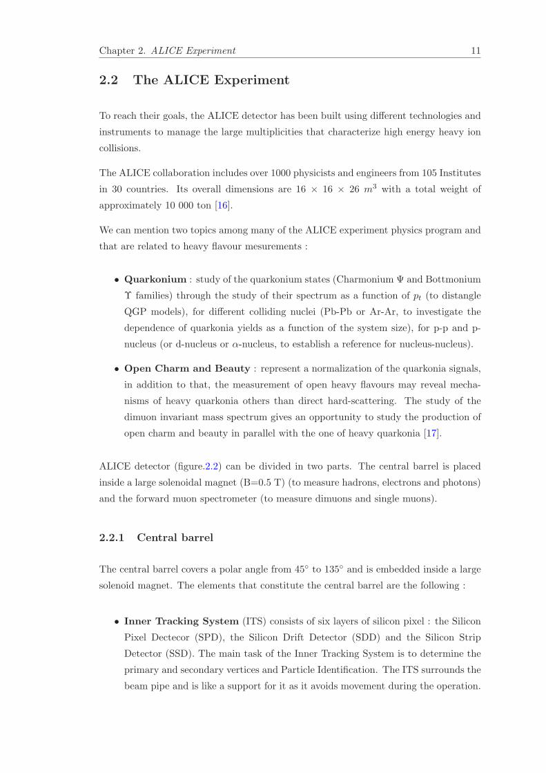
2.2 The ALICE Experiment

To reach their goals, the ALICE detector has been built using different technologies and

instruments to manage the large multiplicities that characterize high energy heavy ion

collisions.

The ALICE collaboration includes over 1000 physicists and engineers from 105 Institutes

in 30 countries. Its overall dimensions are 16 × 16 × 26 m3 with a total weight of

approximately 10 000 ton [16].

We can mention two topics among many of the ALICE experiment physics program and

that are related to heavy flavour mesurements :

• Quarkonium : study of the quarkonium states (Charmonium Ψ and Bottmonium

Υ families) through the study of their spectrum as a function of pt (to distangle

QGP models), for different colliding nuclei (Pb-Pb or Ar-Ar, to investigate the

dependence of quarkonia yields as a function of the system size), for p-p and p-

nucleus (or d-nucleus or α-nucleus, to establish a reference for nucleus-nucleus).

• Open Charm and Beauty : represent a normalization of the quarkonia signals,

in addition to that, the measurement of open heavy flavours may reveal mecha-

nisms of heavy quarkonia others than direct hard-scattering. The study of the

dimuon invariant mass spectrum gives an opportunity to study the production of

open charm and beauty in parallel with the one of heavy quarkonia [17].

ALICE detector (figure.2.2) can be divided in two parts. The central barrel is placed

inside a large solenoidal magnet (B=0.5 T) (to measure hadrons, electrons and photons)

and the forward muon spectrometer (to measure dimuons and single muons).

2.2.1 Central barrel

The central barrel covers a polar angle from 45◦ to 135◦ and is embedded inside a large

solenoid magnet. The elements that constitute the central barrel are the following :

• Inner Tracking System (ITS) consists of six layers of silicon pixel : the Silicon

Pixel Dectecor (SPD), the Silicon Drift Detector (SDD) and the Silicon Strip

Detector (SSD). The main task of the Inner Tracking System is to determine the

primary and secondary vertices and Particle Identification. The ITS surrounds the

beam pipe and is like a support for it as it avoids movement during the operation.


Figure 2.2: The ALICE experiment

The ITS system covers a common range of pseudorapidity |η| < 0.9. The elements

that constitute the ITS are :

- The SPD is the two innermost layers of the ITS, its role is to provide adequate

measurement of the primary and secondary vertex. It also measures the impact

parameter of secondary tracks coming from the weak decay of strange, charm and

beauty particles.

- The SDD is the two intermediate layers of the ITS. The SDD participates in

particle identification by dE/dx technique and reconstructs secondary vertices.

- The SSD is the two outermost layers of the ITS. The SSD is used for matching

tracks from TPC to the ITS and provides 2 dimensional measurement of the track

position and also information on dE/dx which is used for particle identification

[18].

• Time-Projection Chamber (TPC) is the main tracking device in the central

barrel. The TPC performs the tracking and determines the momentum of charged

particles. The range of pseudo-rapidity that the TPC covers is |η| < 0.9. The

coverage range of the transverse momentum is from about 0.1 GeV/c to 100 GeV/c

[19].

• Time-Of-Flight (TOF) has a modular structure that corresponds to 18 sectors

in φ and it covers a cylindrical surface of polar acceptance 45◦ < θ < 135◦ with


pseudorapidity range |η| . 0.9. The TOF measures the time that takes a particle

to travel from the interaction vertex leading to the identification of the particles.

Large samples of pions, kaons and protons are identified thanks to the coupling

between the ITS, the TPC and the TOF [20].

• High-Momentum Particle Idendification Detector (HMPID) measures

Cherenkov radiation (emitted radiation by charged particles at a speed greater

than the velocity of light in the same medium). The aim is to enhance the PID

capability of ALICE by enabling identification of charged hadrons beyond the

momentum interval atteinable (above pt = 1 GeV/c) through energy-loss (in ITS

and TPC) and time-of-flight measurements (in TOF) [21].

• Transition Radiation Detector (TRD) : provides electron identification in the

central barrel for momenta above 1 GeV/c. This is acheived by the conjunction

with the TPC and the ITS through energy loss in pp and Pb-Pb collision. In this

way, the reconstruction of the charm and beauty signal in the semi-leptonic decay

channel is possible [22].

• PHOton spectrometer (PHOS) : it is an electromagnetic calorimeter with high

resolution. Its role is to measure photons that gives information on the temperature

of the system in the initial phase of the collision. The PHOS is made of lead-

tungstate crystal (PbWO4) which is dense and transparent.

• ElectroMagnetic Calorimeter (EMCal): is a large Pb-scintillator sampling

calorimeter with cylindrical geometry adjacent to the ALICE magnet. EMCal

enables ALICE to explore in detail the physics of jet quenching (interaction of

energetic partons with dense matter) over the large energy accessible at the LHC.

It covers |η| ≤ 0.7 and its size is limited by the free space and the maximum weight

that the L3 magnet can support [16].

• Zero Degree Calorimeters (ZDC): measures the remnant of the colliding nuclei

(protons and neutrons which do not participate in the collision). It is located at

110 m on both sides of the interaction point along the beam axis [23].

• T0 : it consists of two arrays of Cherenkov counters (12 counters per array) that

are located on both sides of the interaction point (IP). Its role is to measure with

high precision the time at which the event takes place for the TOF detector. T0

covers a pseudorapidity range −3.3 < η < −2.9 and 4.5 < η < 5.

• Forward Multiplicity Detector (FMD): Its role is to measure charged parti-

cles produced in the collision in the pseudorapidity range −3.4 < η < −1.7 and

1.7 < η < 5.0. The FMD consists of silicon strip channels distributed over 5 ring


counters. It provides information on charged particle multiplicity for all collision

systems. The FMD is limited in space by the presence of the ITS, TPC and muon

arm whose dimensions were decided before those of the FMD.

• V0 : consists of 2 disks of segmented plastic scintillator tiles (named V0A and

V0C) located on both sides of the ALICE collision vertex. It is a small-angle de-

tector with a pseudorapidity coverage similar to the FMD. The principle function

of the V0 detector is to trigger the data taking and determine the centrality of the

event [24].

In general smaller detectors (ZDC, PMD, FMD, T0, V0) are for global event

characterization and triggering the reason for which they are located at small

angles [16, 17, 25].

2.2.2 Forward Muon spectrometer

The second principle part of the ALICE detector is the forward muon spectrometer.

It covers a pseudorapidity range of −4.0 < η < −2.5. The elements that constitute

the muon spectrometer are the dipole magnet, ten planes of trackers and two trigger

chambers and absorbers (front absorber, iron wall, beam shield, rear absorber).

The muon spectrometer measures heavy flavours, quarkonia and light resonances through

their decay into muons and dimuons. So, it is necessary to detail each element of its

constituants and the role of each one [16, 17, 25, 26].

Figure.2.3 contains a layout of the forward muon spectrometer with its different parts:

Figure 2.3: The forward Muon spectrometer layout of main components. An absorberto filter the background, a set of tracking chambers before, inside and after the magnet

and a set of trigger chambers.


2.2.3 Absorbers

A front absorber is located inside the solenoid magnet and it is 4.13 m length. It is

made of carbon and concrete to limit small-angle scattering and energy-loss by traversing

muons. The spectrometer is shielded throughout its length by a dense absorber tube

surrounding the beam pipe. It has a conical geometry to reduce background particle

interaction along the length of the spectrometer. While the front absorber and the beam

shield are sufficient to protect the tracking chambers, additional protection is needed for

the trigger chambers. For this reason the muon filter, i.e. an iron wall 1.2 m thick (∼7.2 λint), is placed after the last tracking chamber, in front of the first trigger chamber.

The front absorber and muon filter stop muons with momentum less than 4 GeV/c.

2.2.4 Tracking system

The tracking system consists of 5 stations each containing two chambers. Each chamber

is below 3% radiation length in terms of thickness. They are made of composite material

to minimize the scattering of the muons so that required resolution is obtained. The 5

stations are based on standard multiwire proportional chambers for which the imposed

constraints are different:

- Stations 1 and 2 cover the smallest surface area in the forward cone and only high

particle densities (up to 4 ×10−2 hits/cm2 for station 1) are observed. The two stations

are placed before of the muon magnet at a distance of ∼ 5.4 m and ∼ 6.8 m respectively

from the IP.

- For station 3, lower particle flux (below 6 × 10−3 hits/cm2) is seen but that station

is located inside the dipole magnet and that helps to minimize the effects of multiple

scattering so that resolution on mass is preserved.

- For stations 4 and 5, they are in the intermediate situation in terms of particle fluxes

and they have very large surface areas.

Stations 3, 4 and 5 are placed at a distance of ∼ 9.7 m (inside the muon magnet), ∼12.65 m and ∼ 14.25 m from the IP. The transverse momentum is determined from the

parameter characterizing the bending plane (|pzy|) after the particles are influenced by

the magnetic field in the third station.


2.2.5 Trigger system

The trigger system is designed to impose selection on tracks and events that will be used

later for analysis. The trigger system consists of 4 planes of Resistive Plate Chambers

that are assembled in 2 stations and located after the passive muon filter. Since there

is important background at low pt, there is a cut imposed on the transverse momentum

of the tracks to reduce background. The two stations are located at about 16 m from

the interaction point and 1 m apart.

2.2.6 Dipole magnet

The dipole magnet is one of the biggest warm dipoles in the world. The overall dimen-

sions of the magnet are 5 m in length, 6.6 m wide, and 8.6 m high. The weight of the

magnet is about 800 t. It is located at 7 m of the interaction point. It is characterized

by a magnetic field of B = 3 Tm field integral. The dipole magnet is also a support for

the muon front absorber and the beam shield.

Chapter 3

Background subtraction

The present analysis is performed using the 2011 proton-proton collisions at 7 TeV

registred by the ALICE experiment. The pt-shape of the background is extracted using

realistic simulations of proton-proton collisions at 7 TeV from 2010 (those of 2011 are not

yet available). The simulations will be introduced with two models of event generators

(PYTHIA and PhoJet). And then, the systematic uncertainties are estimated on each

step of the subtraction procedure.

3.1 Realistic simulations

(GeV/c)T

p0 5 10 15 20 25 30

(C

ount

s /

0.5

GeV

/c)

TdpdN

1

10

210

310

410

510

610

pp 7 TeV PYTHIA - Muon track sources - No cuts

All tracksMu from primaryMu from secondaryMu from charmMu from beautyHadronsFakes

(GeV/c)T

p0 5 10 15 20 25 30

(C

ount

s /

0.5

GeV

/c)

TdpdN

1

10

210

310

410

510

610

pp 7 TeV PYTHIA - Muon track sources - With cuts

All tracksMu from primaryMu from secondaryMu from charmMu from beautyHadronsFakes

Figure 3.1: Transverse momentum ditributions of muon track sources in pp collisionsat

√s = 7 TeV obtained from simulations with PYTHIA, without (left) and with (right)

event and track selection.

17

Chapter 3. Results 18

Figure 3.2: The production mechanisms for different muon track sources.

Realistic simulations (figure.3.1) show that muons detected in the muon spectrometer

are coming from different sources. The left panel of figure.3.1 shows the pt-spectrum of

muon tracks reconstructed in the muon spectrometer without any selection cuts.

There are muons from Open Heavy Flavour decay (charm and beauty). They have short

lifetime and they decay directly after their production into single muons as it is shown

in figure 3.2.

Muons from light hadrons decay which primary K/π are the most dominant (as it

is shown in appendix.A). The production of those muons depends on the distance

travelled by kaons and pions after their production in pp collision before reaching the

front absorber.

But not all light hadrons decay into muons before the front absorber. Actually, some of

them reach the front absorber and interact with it to produce muons. The production of

these secondary muons depends on the interaction probability with the front absorber.

In the spectrum, there are also hadrons which were misidentified as muons and fake

tracks resulting from the noise of the detector. The inclusive muon spectrum is also

shown in the same figure and it represents muons from all muon sources.

The pt-spectrum of muons from realistic simulation that will be used is the one obtained

after applying the selection cuts (see right panel of figure.3.1).

The selected events have at least one reconstructed interaction vertex. Various track

cuts were applied in order to further reduce the background contributions in the data

sample.

• Tracks were required to be reconstructed in the geometrical acceptance of the

muon spectrometer, with −4.0 < η < −2.5 and 171◦ < θabs < 178◦, θabs being the

track polar angle measured at the end of the absorber.


• Then, the track candidate measured in the muon tracking chambers was required

to be matched with the corresponding one measured in the trigger chambers. This

results in a very effective rejection of the hadronic component that is absorbed in

the iron wall.

• The correlation between momentum and Distance of Closest Approach (DCA,

distance between the extrapolated muon track and the interaction vertex, in the

plane perpendicular to the beam direction and containing the vertex) was used

to remove remaining beam-induced background tracks which do not point to the

interaction vertex. Indeed, due to the multiple scattering in the front absorber,

the DCA ditribution of tracks coming from the interaction vertex is expected to be

described by a Gaussian function whose width depends on the absorber material

and is proportional to 1/p. The beam-induced background does not follow this

trend and can be rejected by applying a cut on p× DCA at 5 σ. The width is

extracted from a Gaussian fit to the p × DCA distribution measured in two regions

in θabs, corresponding to different materials in the front absorber.

By comparing the spectra with and without selection cuts, one can notice that all fake

tracks are suppressed for pt > 5 GeV/c, hadrons also are suppressed for pt & 10 GeV/c.

So hadrons and fake tracks are reduced partially after applying selection cuts. The main

background source is the primary muons while the amount of secondaries, hadrons and

fakes are negligible.

3.2 pT -shape of the background

In our study, we will focus on the range of pt > 2 GeV/c, because the dominant back-

ground which is muons coming from primary K/π is dominant in the range 0 < pt < 2

GeV/c, with respect to the signal in interest which is muons from heavy flavours.

The background which will be subtracted is the muons from primaries. Its pT -shape

had to be extracted from realistic simulation using the same selection cuts applied on

the real data. Then, the obtained pt-shape of background is normalized to the real data

to estimate the background. After subtracting the background, we are left with the

spectrum of muons from open heavy flavour.

To obtain pt-shape, spectrum of primary muons is fitted using the function defined by

the equation.3.1

f(pT ) =A

(B2 + p2t )n

(3.1)

where A, B and n are free parameters.


(GeV/c)T

p2 4 6 8 10 12 14 16 18 20

Cou

nts

/ 0.

5 G

eV/c

-310

-210

-110

1

10

210

310

410

MC input

fit

< -2.5η-2.8 <

(GeV/c)T

p2 4 6 8 10 12 14 16 18 20

Cou

nts

/ 0.

5 G

eV/c

-310

-210

-110

1

10

210

310

410

MC input

fit

< -2.5η-2.8 <

(GeV/c)T

p2 4 6 8 10 12 14 16 18 20

Cou

nts

/ 0.

5 G

eV/c

-310

-210

-110

1

10

210

310

410

MC input

fit

< -2.8η-3.1 <

(GeV/c)T

p2 4 6 8 10 12 14 16 18 20

Cou

nts

/ 0.

5 G

eV/c

-310

-210

-110

1

10

210

310

410

MC input

fit

< -2.8η-3.1 <

(GeV/c)T

p2 4 6 8 10 12 14 16 18 20

Cou

nts

/ 0.

5 G

eV/c

-310

-210

-110

1

10

210

310

410

MC input

fit

< -3.1η-3.4 <

(GeV/c)T

p2 4 6 8 10 12 14 16 18 20

Cou

nts

/ 0.

5 G

eV/c

-310

-210

-110

1

10

210

310

410

MC input

fit

< -3.1η-3.4 <

(GeV/c)T

p2 4 6 8 10 12 14 16 18 20

Cou

nts

/ 0.5

GeV

/c

-410

-310

-210

-110

1

10

210

310

410

MC input

fit

< -3.4η-3.7 <

(GeV/c)T

p2 4 6 8 10 12 14 16 18 20

Cou

nts

/ 0.

5 G

eV/c

-310

-210

-110

1

10

210

310

410

MC input

fit

< -3.4η-3.7 <

(GeV/c)T

p2 4 6 8 10 12 14 16 18 20

Cou

nts

/ 0.

5 G

eV/c

-310

-210

-110

1

10

210

310

410

MC input

fit

< -3.7η-4.0 <

(GeV/c)T

p2 4 6 8 10 12 14 16 18 20

Cou

nts

/ 0.

5 G

eV/c

-310

-210

-110

1

10

210

310

410

MC input

fit

< -3.7η-4.0 <

Figure 3.3: Fit and extrapolation of the primary muons pt-spectrum in the 5η binsusing PYTHIA (left) and PhoJet (right).


But this is not sufficient since primary muons spectrum is up to 12 GeV/c (after selection

cuts, statistics of primary muons are not large enough) while that of inclusive muons

from real data is up to 20 GeV/c. An extrapolation up to 20 GeV/c is required using

the same previous function for fit. The fit and extrapolation in each η bin is shown in

figure.3.3.

The procedure of fitting and extrapolation at high pt may influence the results intro-

ducing additional systematic uncertainties on background estimation. For that reason

and before going ahead the validation of the stability of the procedure should be done.

We perform the following cross-check for both PYTHIA and PhoJet :

1. We divide the total acceptance in pseudorapidity (−4.0 < η < −2.5) into 5 equally

sized bins.

2. Fit the primary muons pt-spectrum from 2 to 20 GeV/c in each pseudorapidity

bin and sum over the 5 bins to get the pt-spectrum of primary muons in the total

η region.

3. Fit the pt-spectrum of primary muons in the total acceptance.

4. Compare results from steps 2 and 3.

(GeV/c)T

p2 4 6 8 10 12 14 16 18 20

Cou

nts

/ 0.

5 G

eV/c

-210

-110

1

10

210

310

410fit primary_PYTHIA muons in LHC10f6a

Mu from primary_PYTHIA

fit sum_PYTHIA

total fit_PYTHIA

< -2.5η-4.0 <

(GeV/c)T

p2 4 6 8 10 12 14 16 18 20

Cou

nts

/ 0.

5 G

eV/c

-210

-110

1

10

210

310

410fit primary_PhoJet muon in LHC10f6

Mu from primary_PhoJet

fit sum_PhoJet

total fit_PhoJet

< -2.5η-4.0 <

Figure 3.4: Comparison between the pT -shape of primary muons in the total accepat-nce −4.0 < η < −2.5 (red line) and the sum from the fit in the 5 pseudo-rapidity bins

(green lines). Left panel : PYTHIA. Right panel : PhoJet.

The comparisons of the resulting fits are shown in figure.3.4. The green curve is the

sum of the fit from the 5 pseudo-rapidity bins individually and the red curve is the fit

in the total acceptance. The comparison between both shows that they are compatible

with each other, but there is a slight difference at high pt for PYTHIA, which could be

explained due to the fact that there is not enough statistics. In addition to that, the


background at high pt-region is small with respect to the signal, so the signal is weakly

affected by the background at high pT . The strategy of fit and extrapolation to extract

the pT -shape of the background is then stable and the procedure is validated.

3.3 Background Normalization

The statistics in real data and in simulations are different. To perform the subtraction,

pt-shapes of the background from simulations should be scaled to real data. For this

purpose, scaling factors (defined by the equation.3.2) are calculated to perform the nor-

malization of spectrum from simulations. The background pt-shape is then subtracted

from the pt-spectrum of real data.

SMC(∆η) = RMC(∆η)×N inclusiveµ

RD (lowpt,∆η)

NprimaryµMC (lowpt,∆η)

(3.2)

where the factor RMC is the ratio between the yield of primary and inclusive muons in

the same ∆η region and it is represented by the equation.3.3,

RMC(∆η) =Nprimaryµ

MC (lowpt,∆η)

N inclusiveµMC (lowpt,∆η)

=Nprimaryµ

RD (lowpt,∆η)

N inclusiveµRD (lowpt,∆η)

(3.3)

such that,

Ninclusiveµ/primaryµRD/MC (pt,∆η) =

∫∆η

dη

∫ 1GeV/c

0dpt

d2N inclusiveµ/primaryµ

dptdη(3.4)

where N is the number of muon tracks (primary or inclusive) with 0 < pt < 1 GeV/c

(where the background is dominant) in a given ∆η region from data or simulations.

Using the expression of RMC and SMC(∆η) defined by the equation.3.3 and equation.3.2

respectively, the final expression of the scaling factors that were used for normalization

is represented by the equation.3.5.

SMC(∆η) =N inclusiveµ

RD (lowpt,∆η)

N inclusiveµMC (lowpt,∆η)

(3.5)

There is a scaling factor computed for each η-bin and for each model, to scale the pt-

spectrum extracted of primary muons in each ∆η region so that we could estimate the


(GeV/c)T

p2 4 6 8 10 12 14 16 18 20

µ /

tota

l µ

prim

ary

0

0.05

0.1

0.15

0.2

0.25

0.3

0.35

0.4

0.45

0.5

Ratio_PYTHIA_MC in Eta 1

Ratio_PhoJet_MC in Eta 1

Ratio_PYTHIA_RD in Eta 1

Ratio_PhoJet_RD in Eta 1

< -2.5η-2.8 <

(GeV/c)T

p0 2 4 6 8 10 12 14 16 18 20

(C

ount

s /

0.5

GeV

/c)

Tdp

trk

dN

1

10

210

310

410

510

610

All tracks in Eta1- Real Data

All tracks in Eta 1 PYTHIA

All tracks in Eta 1 PhoJet

< -2.5η-2.8 <

(GeV/c)T

p2 4 6 8 10 12 14 16 18 20

µ /

tota

l µ

prim

ary

0

0.05

0.1

0.15

0.2

0.25

0.3

0.35

0.4

0.45

0.5





< -2.8η-3.1 <

(GeV/c)T

p0 2 4 6 8 10 12 14 16 18 20

(C

ount

s /

0.5

GeV

/c)

Tdp

trk

dN

1

10

210

310

410

510

610All tracks in Eta2 - Real Data



< -2.8η-3.1 <

(GeV/c)T

p2 4 6 8 10 12 14 16 18 20

µ /

tota

l µ

prim

ary

0

0.05

0.1

0.15

0.2

0.25

0.3

0.35

0.4

0.45

0.5





< -3.1η-3.4 <

(GeV/c)T

p0 2 4 6 8 10 12 14 16 18 20

(C

ount

s /

0.5

GeV

/c)

Tdp

trk

dN

1

10

210

310

410

510

610All tracks in Eta3 - Real Data



< -3.1η-3.4 <

(GeV/c)T

p2 4 6 8 10 12 14 16 18 20

µ /

tota

l µ

prim

ary

0

0.05

0.1

0.15

0.2

0.25

0.3

0.35

0.4

0.45

0.5





< -3.4η-3.7 <

(GeV/c)T

p0 2 4 6 8 10 12 14 16 18 20

(C

ount

s /

0.5

GeV

/c)

Tdp

trk

dN

1

10

210

310

410

510

610

All tracks in Eta 4 - Real Data



< -3.4η-3.7 <

(GeV/c)T

p2 4 6 8 10 12 14 16 18 20

µ /

tota

l µ

prim

ary

0

0.05

0.1

0.15

0.2

0.25

0.3

0.35

0.4

0.45

0.5





< -3.7η-4.0 <

(GeV/c)T

p0 2 4 6 8 10 12 14 16 18 20

(C

ount

s /

0.5

GeV

/c)

Tdp

trk

dN

1

10

210

310

410

510

610

All tracks in Eta 5 - Real Data



< -3.7η-4.0 <

Figure 3.5: Estimated ratio of primaries (scaled) to inclusive muons for real data andMonte Carlo simulations (left) and comparison between the inclusive spectrums of real

data and Monte Carlo simulations (right) in the 5 η bins.


(GeV/c)T

p2 4 6 8 10 12 14 16 18 20

µ /

tota

l µ

prim

ary

0

0.05

0.1

0.15

0.2

0.25

0.3

0.35

0.4

0.45

0.5Ratio_PYTHIA_MC_All

Ratio_PhoJet_MC_All

Ratio_PYTHIA_RD_All

Ratio_PhoJet_RD_All

< -2.5η-4.0 <

(GeV/c)T

p0 2 4 6 8 10 12 14 16 18 20

(Cou

nts

/ 0.

5 G

eV/c

) T

dptrk

dN

10

210

310

410

510

610

All tracks - Real Data

All tracks PYTHIA

All tracks PhoJet

< -2.5η-4.0 <

Figure 3.6: The same as figure.3.5 in −4.0 < η < −2.5.

yield of primary muons in real data. The scaling factors obtained for each η bin and for

each model are presented in Appendix.B.

The left panel of figure.3.6 represents the ratios between primary and inclusive muons,

this is, the estimated background in data and in simulations in the total acceptance.

The primary muons spectrum is already scaled with SMC(∆η). It is noticed that the

estimated background is decreasing with increasing pt. That behaviour is the same more

or less in the four curves. The background is important at low pt approximately up to

25% for real data but at high pt the background is small. It is possible to say that the

signal is less sensitive to the background at high-pt while at low pT , the signal is much

more contaminated with respect to high pT .

The right panel of figure.3.6 represents the pt spectrum of inclusive muons from real

data and from simulation for different models. One can notice that the behaviour of pt

spectrum of muons is similar between real data and Monte Carlo simulation, there is

only a difference in yield.

The pt spectrum of muons from data and simulations and the estimated background in

each η bin are also shown (see figure.3.5).

3.4 Results

After the calculation of the scaling factors and normalizing the primary muon spectrum

to the real data, the ratio of primary muons (background) is estimated in real data and


(GeV/c)T

p2 4 6 8 10 12 14 16 18 20

(C

ount

s /

0.5

GeV

/c)

Tdp

trk

dN

10

210

310

410

510

Signal before subtraction

Mean Signal after subtraction

< -2.5η-4.0 <

η-4 -3.8 -3.6 -3.4 -3.2 -3 -2.8 -2.6

Muo

n Y

ield

100

150

200

250

300

350

4003

10×

Muon Yield before subtraction

Muon Yield after subtraction

< -2.5η-4.0 <

Figure 3.7: Left panel : yield of muons before background subtraction and the meanyield after the background subtraction from PYTHIA and PhoJet as a function of pT in−4.0 < η < −2.5. Right panel : yield of muons before and after background subtraction

as a function of η and for 2 < pT < 20 GeV.

in simulations. The subtraction of the background is performed and we obtain the pT -

spectrum of muons from heavy flavour decay (see left panel of figure.3.7) and the η-yield

of muons from open heavy flavour decay (right panel of figure.3.7). The final signal

is the average coming from the two signals obtained using the two estimated primary

muon spectrum from different simulation models.

3.5 Systematic uncertainties

Systematic uncertainties arise from different steps in the procedure followed to subtract

the background. First, we have fitted and extrapolated the pt-spectrum of the primary

muons from realistic simulations and from that procedure we can ignore the systematic

uncertainties. The following step was the subtraction where two background shapes were

used, then there is an uncertainty due to the different models σmodel. Next, the pt-shapes

of the background were normalized to real data. The normalization is influenced by the

different transport processes that introduce an other kind of uncertainties (σnorm).

We begin by σmodel which is simple to find. The signal is obtained after subtraction

using the two models. The mean value of the two previous signals is computed in the

total acceptance and in each η-bin separately. The average gives the central value of the

muons signal and σmodel is given by the ratio between the average spectrum and the two

signals obtained after background subtraction using PYTHIA and PhoJet. The ratio

is shown in the left panel of figures.3.8 in the 5 η bins. This systematic uncertainty is

relatively small and we can consider that it does not depend on pt, but only on the η

bin. For this reason, σmodel is taken to be the maximum deviation in each η bin.


(GeV/c)T

p2 4 6 8 10 12 14 16 18 20

Rat

io

0.5

0.6

0.7

0.8

0.9

1

1.1

1.2

1.3

1.4

1.5

Ratio_Model from LHC10f6a in Eta 1

Ratio_Model from LHC10f6 in Eta 1

< -2.5η-2.8 <

(GeV/c)T

p2 4 6 8 10 12 14 16 18 20

Rat

io

0.5

0.6

0.7

0.8

0.9

1

1.1

1.2

1.3

1.4

1.5

Ratio_Norm from LHC10f6a in Eta 1Ratio_Norm from LHC10f6 in Eta 1

< -2.5η-2.8 <

(GeV/c)T

p2 4 6 8 10 12 14 16 18 20

Rat

io

0.5

0.6

0.7

0.8

0.9

1

1.1

1.2

1.3

1.4

1.5



< -2.8η-3.1 <

(GeV/c)T

p2 4 6 8 10 12 14 16 18 20

Rat

io

0.5

0.6

0.7

0.8

0.9

1

1.1

1.2

1.3

1.4

1.5

Ratio_Norm from LHC10f6a in Eta 2

Ratio_Norm from LHC10f6 in Eta 2

< -2.8η-3.1 <

(GeV/c)T

p2 4 6 8 10 12 14 16 18 20

Rat

io

0.5

0.6

0.7

0.8

0.9

1

1.1

1.2

1.3

1.4

1.5



< -3.1η-3.4 <

(GeV/c)T

p2 4 6 8 10 12 14 16 18 20

Rat

io

0.5

0.6

0.7

0.8

0.9

1

1.1

1.2

1.3

1.4

1.5

Ratio_Norm from LHC106fa in Eta 3


< -3.1η-3.4 <

(GeV/c)T

p2 4 6 8 10 12 14 16 18 20

Rat

io

0.5

0.6

0.7

0.8

0.9

1

1.1

1.2

1.3

1.4

1.5



< -3.4η-3.7 <

(GeV/c)T

p2 4 6 8 10 12 14 16 18 20

Rat

io

0.5

0.6

0.7

0.8

0.9

1

1.1

1.2

1.3

1.4

1.5



< -3.4η-3.7 <

(GeV/c)T

p2 4 6 8 10 12 14 16 18 20

Rat

io

0.5

0.6

0.7

0.8

0.9

1

1.1

1.2

1.3

1.4

1.5

Ratio_Model from LHC10f6a in Eta 5Ratio_Model from LHC10f6 in Eta 5

< -3.7η-4.0 <

(GeV/c)T

p2 4 6 8 10 12 14 16 18 20

Rat

io

0.5

0.6

0.7

0.8

0.9

1

1.1

1.2

1.3

1.4

1.5



< -3.7η-4.0 <

Figure 3.8: Estimated systematic uncertainties for σmodel (left) and σnorm (right) inthe 5 η bins.


(GeV/c)T

p2 4 6 8 10 12 14 16 18 20

Rat

io

0.5

0.6

0.7

0.8

0.9

1

1.1

1.2

1.3

1.4

1.5

Ratio_Model from LHC10f6a total

Ratio_Model from LHC10f6 total < -2.5η-4.0 <

(GeV/c)T

p2 4 6 8 10 12 14 16 18 20

Rat

io

0.5

0.6

0.7

0.8

0.9

1

1.1

1.2

1.3

1.4

1.5

Ratio_Norm from LHC10f6a total

Ratio_Norm from LHC10f6 total < -2.5η-4.0 <

Figure 3.9: Estimated systematic uncertainties for σmodel (left) and σnorm (right) inthe total acceptance.

For σnorm, it is not straightforward. The uncertainty is due to normalization. The

transport codes (GEANT3 and Fluka) used in Monte Carlo simulations do not give

the same yield of secondary muons that are produced inside the front absorber. It is

assumed that the difference in secondary yield between the transport processes is 100%

which means that two cases are considered : no secondary muons or two times more

secondary muons. The variation of the secondary yields influences inclusive muon yields

and as a consequence the normalization will be different. So, new scaling factors had

to be calculated (see Appendix.B). The systematic uncertainty is given by the ratio

between the spectrum with the new scaling factors and the original one for each model

and for each η bin.

According to the right panel of figure.3.8, σnorm does not depend on η bin only but also

on each pt value. One can also notice that σnorm is not small as in σmodel.

Results on systematic uncertainties are shown in figure.3.8 and the corresponding values

of uncertainties are introduced in table.3.1.

Systematic uncertaities in the total η region were also calculated and presented in ta-

ble.3.1. The associated ratios are shown in figure.3.9.

Chap

ter3.

Results

28

Table3.1:Estim

ated

system

atic

uncertainties

forσm

odelan

dσnorm.

σmodel σnorm

pt (GeV/c)

2-2.5 2.5-3 3-3.5 3.5-4 4-4.5 4.5-5 5-5.5 5.5-6 6-6.5 6.5-7 7-7.5 7.5-8 8-8.5 8.5-9 9-9.5 10-20

2.5 < η < 4.0 2% 9% 8% 7% 6% 5% 4% 3.5% 3% < 3%

2.5 < η < 2.8 3% 17% 14% 13% 12% 11% 10% 9% 8.5% 8% 7.5% 7% 7% 7% 7% 6% < 6%

2.8 < η < 3.1 7% 22% 19.5% 16% 13% 12% 10% 9% 8% 7% 6% 6% 5.5% 5% 5% 4% < 4%

3.1 < η < 3.4 3.5% 13% 12% 9.5% 8% 6% 5% 4% < 4%

3.4 < η < 3.7 2.5% 6% 5% 4% < 4%

3.7 < η < 4.0 2.5% 3%

Chapter 4

Conclusion

Heavy flavours are produced in the early stages of heavy ion collisions making them

good probes for the Quark Gluon Plasma. In proton-proton collisions, heavy flavours

can also be used to test perturbative QCD calculations. In addition to that, their study

is of great importance because they are a natural normalization in the study of heavy

ion collisions.

The ALICE experiment studies quarkonia and open heavy flavour at mid and forward

rapidity. The muon spectrometer measures single muons from open heavy flavour decay

and dimuons from quarkonia decay in a pseudorapidity coverage of −4.0 < η < −2.5.

The pt spectrum of inclusive muons detected with the muon spectrometer contains dif-

ferent muon sources. In order to subtract the background, muons from light hadron

decays, the pt-shape was determined using realistic simulations with different event gen-

erators using fit and extrapolation strategy. The subtraction was performed in the range

2 < pt < 20 GeV/c since the background is dominant in the range [0,2] GeV/c. The

resulting pt spectrum was scaled to real data to estimate the background. Then, the

background was subtracted using two diffrent models to obtain the final signal of open

heavy flavour given by the average of the two signals obtained after background subtrac-

tion. Systematic uncertainties were estimated on each step of the subtraction procedure.

The uncertainties on the fit and extrapolation has been assumed to be negligible. Un-

certainties from models were found to be small and η dependent. Uncertainties from

normalization were found to be important and depend on both pt and η.

29

Appendix A

π/K Dominant Primary particles

In the present appendix, we are presenting in tables from A.1 to A.6, the main sources

of muons coming from light hadron decay, charm and beauty hadrons decay.

Two event generators were used. For each, rounded percentages of each particle that

contributes in the muon spectrum are presented in these tables. Such an example, ta-

ble.A.1 and table.A.4 are presenting the percentages of light hadrons that have decayed

into muons from PYTHIA and PhoJet. From table.A.1, one can notice that the per-

centage of Kaons and pions together is approximately 63%. Then, dominant primary

particles decaying into muons are pions and kaons.

Rounded percentages for muons coming from charm and beauty particles can be found

in table.A.2 and table.A.3.

The percentage of primaries and open heavy flavours could be extracted from simulations

using PhoJet also. The rounded values are presented in table.A.4 for light hadrons and

table.A.6 for beauty particles and table.A.5 for charm particles.

Table A.1: Produced primary particles according to PYTHIA

Muons from primary

PDG code Particle Pourcentage

211 π+ 33 %

321 K+ 22 %

113 ρ0(770) 11 %

213 ρ0(770) 10 %

313 K∗0(892) 8 %

31

Appendix A. Dominant primary particles 32

Table A.2: Produced open charm particles according to PYTHIA

Muons from Charm


411 D+ 37 %

413 D∗+(2010) 24 %

423 D∗0(2007) 16 %

421 D0 14 %

433 D∗+s 3 %

Table A.3: Produced open beauty particles according to PYTHIA

Muons from Beauty


513 B∗0 25 %

511 B0 21 %

523 B∗+ 22 %

521 B+ 19 %

533 B∗0s 4 %

Table A.4: Produced primary particles according to PhoJet

Muons from primary


211 π+ 28 %

213 ρ+(770) 11 %

113 ρ0(770) 12 %

313 K∗0(892) 13 %

321 K+ 16 %

323 K∗+(892) 8 %

Table A.5: Produced open charm particles according to PhoJet

Muons from Charm


421 D0 49 %

411 D+ 42 %

431 D+s 8 %

Appendix A. Dominant primary particles 33

Table A.6: Produced open beauty particles according to PhoJet

Muons from Beauty


511 B0 46 %

521 B+ 44 %

531 B0s 7 %

Appendix B

Scaling factors

In this appendix, values of the scaling factors are given for the 5 η bins and for the total

η region for each simulation model. Those values are used to scale the pt-shape of the

background (primary muons) to real data.

The final expression to compute the scaling factors is defined by the equation.3.5 assum-

ing that the expression is valid only at low pt (pt < 1 GeV/c) where the background is

dominant.

The obtained rounded values are summarized in table.B.1.

We also show the scaling factors used to determine the systematic uncertainties in the

case of σnorm. Indeed, as mentioned in chapter 3, the number of muons coming from

Table B.1: Scaling factors (rounded) used to scale the background to the real data

pseudorapidity Scaling factor

PYTHIA PhoJet

−4.0 < η < −2.5 50 42

−2.8 < η < −2.5 56 53

−3.1 < η < −2.8 57 51

−3.4 < η < −3.1 50 42

−3.7 < η < −3.4 47 39

−4.0 < η < −3.7 46 38

35

Appendix B. Scaling factors 36

Table B.2: Scaling factors used for background subtraction and to compute σnorm.

Scaling factor

Pseudorapidity PYTHIA PhoJet

2* secondary muons original 0* secondary muons 2* secondary muons original 0* secondary muons

−4.0 < η < −2.5 41 50 63 35 42 54

−2.8 < η < −2.5 45 56 73 42 53 70

−3.1 < η < −2.8 45 57 77 40 51 71

−3.4 < η < −3.1 39 50 68 33 42 59

−3.7 < η < −3.4 39 47 57 32 39 49

−4.0 < η < −3.7 41 46 52 34 38 43

secondary particles depends on the transport of particles through the material. So σnorm

takes into account this dependence by varying, within 100%, the amount of secondary

muons extracted with the different event generators. This leads to the fact that the

inclusive number of muons would be changed and consequently the scaling factors. It

means that there are two cases to consider when calculating the new scaling factors.

One case is to consider that there is no secondary muons and the second case is that

there are two times more secondary muons.

Bibliography

[1] Diego Stocco. Development of the ALICE Muon Spectrometer: preparation for data

taking and heavy flavor measurement. PhD thesis, Universita degli Studi di Torino,

2008.

[2] Francesco Prino. Open heavy flavour reconstruction in the alice central barrel.

ICHEP08, arXiv:0810.3086, 2008.

[3] Francois Gelis. Some aspects of ultra-relativistic heavy ion collisions. Acta

Phys.Polon.Supp., 1:395–402, 2008.

[4] M. A. Stephanov. Non-gaussian fluctuations near the qcd critical points. Phys.

Rev. Lett., 102:0323301, Jan 2009.

[5] A. Andronic, F. Beutler, P. Braun-Munzinger, K. Redlich, and J. Stachel. Statistical

hadronization of heavy flavor quarks in elementary collisions: Successes and failures.

Phys.Lett., B678:350–354, 2009.

[6] Lizardo Valencia Palomo. Inclusive J/ψ production measurement in Pb-Pb col-

lisions at√sNN = 2.76TeV with the ALICE Muon Spectrometer. PhD thesis,

Paris-sud University & IPN, 2013.

[7] M. Lunardon. Open heavy flavour detection in ALICE. Nucl.Phys.Proc.Suppl., 167:

25–28, 2007.

[8] A. Adare et al. Energy loss and flow of heavy quarks in au-au collisions at√sNN

= 200 gev. Phys.Rev.Lett, 98:172301, 2007.

[9] Serhiy Senyukov. Open heavy flavour analysis with the alice experiment at

lhc,arxiv:1304.2189v1. Phys.Lett., 2013.

[10] A Dainese. Measurement of heavy-flavour production in proton-proton collisions at√s = 7 tev with alice. arXiv:1012.4036, 2010.

[11] Betty Abelev et al. Heavy flavour decay muon production at forward rapidity in

proton-proton collisions at√s = 7 tev. Phys.Lett., B708:265–275, 2012.

37

Bibliography 38

[12] Xiaoming Zhang. Study of Heavy Flavours from Muons Measured with the AL-

ICE Detector in Proton–Proton and Heavy-Ion Collisions at the CERN-LHC. PhD

thesis, CENTRAL CHINA NORMAL UNIVERSITY and BLAISE PASCAL UNI-

VERSITY, 2012.

[13] Philip Bryant for the ALICE Collaboration Lyndon Evans. The cern large hadron

collider: Accelerator and experiments, lhc machine. Journal of Instrumentation, 3:

158, 2008.

[14] 2014. URL http://home.web.cern.ch/topics/large-hadron-collider.

[15] 2014. URL http://home.web.cern.ch/about/experiments.

[16] ALICE Collaboration. The cern large hadron collider: Accelerator and experiment,

the alice experiment at the cern lhc. Journal of Instrumentation, 3:245, 2008.

[17] 2008. URL http://aliceinfo.cern.ch/Public/en/Chapter2/Chap2_dim_spec.html.

[18] ALICE Collaboration. Alice, technical design report of the inner tracking system

(its). ALICE-DOC-2005-002 v.1, 2003.

[19] ALICE Collaboration. Alice, technical design report of the time projection chamber.

ALICE-DOC-2003-011, 2003.

[20] ALICE Collaboration. Alice, addendum to the technical design report of the time

of flight system (tof). ALICE-DOC-2004-002 v.1, 2004.

[21] ALICE Collaboration. Alice, technical design report of the high momentum particle

identification detector. ALICE-DOC-1998-01 v.1, 2001.

[22] ALICE Collaboration. Alice, technical design report of the transition radiation

detector. ALICE-DOC-2004-009 v.1, 2004.

[23] ALICE Collaboration. Alice, technical design report of the zero degree calorimeter

(zdc). ALICE-DOC-2004-003 v.1, 1999.

[24] ALICE Collaboration. Alice, technical design report on forward detectors: Fmd,

t0 and v0. ALICE-DOC-2004-010 v.1, 2004.

[25] ALICE Collaboration. Alice, technical design report of the dimuon forward spec-

trometer. ALICE-DOC-2004-004 v.1, 2004.

[26] Gines Martinez. Physics of the muon spectrometer of the ALICE experiment.

J.Phys.Conf.Ser., 50:361–370, 2006.

http://home.web.cern.ch/topics/large-hadron-collider

http://home.web.cern.ch/about/experiments

http://aliceinfo.cern.ch/Public/en/Chapter2/Chap2_dim_spec.html

background subtraction for open heavy avour studies in proton-proton ... · pdf filebackground...

Documents