background facts: consistent seasonal adjustment · 2018-08-21 · anders wallgren and britt...

www.scb.se Arbetsmarknads- och utbildningsstatistik

ISSN 1103-7458

Bakgrundsfakta

Statistikpublikationer kan beställas från SCB, Publikationstjänsten, 701 89 ÖREBRO, e-post: [email protected],telefon: 019-17 68 00, fax: 019-17 64 44. De kan också köpas genom bokhandeln eller direkt hos SCB, Karlavägen 100 i Stockholm. Aktuell publicering redovisas på vår webbplats (www.scb.se). Ytterligare hjälp ges av Information och bibliotek, e-post: [email protected], telefon: 08-506 948 01, fax: 08-506 948 99.

Statistical publications can be ordered from Statistics Sweden, Publication Services, SE-701 89 ÖREBRO, Sweden (phone: +46 19 17 68 00, fax: +46 19 17 64 44, e-mail: [email protected]). If you do not find the data you need in the publications, please contact Statistics Sweden, Information and Library, Box 24300, SE-104 51 STOCKHOLM, Sweden (e-mail: [email protected], phone: +46 8 506 948 01, fax: +46 8 506 948 99).

2013:3

Consistent Seasonal Adjustment and

Trend-cycle Estimation

The series Background facts presents background material for statistics produced by the Department of Labour and Education Statistics at Statistics Sweden. Product descriptions, methodology reports and various statistic compilations are examples of background material that give an overview and facilitate the use of statistics.

Publications in the series Background facts on Labour and Education Statistics

2000:1 Övergång till yrkeskodning på fyrsiffernivå (SSYK) och införande av jobbstatus- kod i SCB:s lönestatistik

2000:2 The Information System for Occupational Injuries and the Work-related Health Problems Survey – A comparative study

2000:3 Konferens om utbildningsstatistik den 23 mars 2000

2001:1 Avvikelser i lönesummestatistiken – en jämförelse mellan LAPS och LSUM

2001:2 En longitudinell databas kring utbildning, inkomst och sysselsättning 1990–1998 2001:3 Staff training costs 1994–1999

2001:4 Studieresultat i högskolan i form av avklarade poäng

2001:5 Urvals- och estimationsförfarandet i de svenska arbetskraftsundersökningarna (AKU)

2001:6 Svar, bortfall och representativitet i Arbetsmiljöundersökningen 1999

2001:7 Individ- och företagsbaserad sysselsättningsstatistik – en jämförelse mellan AKU och KS

2002:1 Tidsseriebrott i utbildningsregistret 2001-01-01

2002:2 En longitudinell databas kring utbildning, inkomst och sysselsättning (LOUISE) 1990–1999

2003:1 Exempel på hur EU:s ”Quality Reports” kan skrivas – avser Labour Cost Survey (LSC) 2000 2003:2 Förändrad redovisning av högskolans personal

2003:3 Individ- och företagsbaserad sysselsättningsstatistik – en fortsatt jämförelse mellan AKU och KS

2003:4 Sjukfrånvarande enligt SCB och sjukskrivna enligt RFV

2003:5 Informationssystemet om arbetsskador och undersökningen om arbetsorsakade besvär. En jämförande studie 2004:1 Samlad statistik från SCB avseende ohälsa

2004:2 Översyn av forskarutbildningsstatistiken. Bedömning av kvaliteten

2004.3 Sjukfrånvaro och ohälsa i Sverige – en belysning utifrån SCB:s statistik

2005:1 En longitudinell databas kring utbildning, inkomst och sysselsättning (LOUISE) 1990–2002

2005:2 Nordisk pendlingskarta. Huvudrapport 2005:3 Nordisk pendlingskarta. Delrapport 1–4.

2005:4 Flödesstatistik från AKU

2005:5 Flow statistics from the Swedish Labour Force Survey

2006:1 Sysselsättningsavgränsning i RAMS – Metodöversyn 2005

Continued on inside of the back cover!

Background Facts

Consistent Seasonal Adjustment and

Trend-cycle Estimation

Labour and Education Statistics 2013:3

Statistics Sweden 2013

Background Facts Labour and Education Statistics 2013:3

Consistent Seasonal Adjustment and Trend-cycle Estimation Statistics Sweden 2013 Producer Statistics Sweden, Population and Welfare Department BOX 24300 SE-104 51 STOCKHOLM Inquires Daniel Samuelsson +46 8 506 949 78 [email protected]

Elisabet Andersson +46 8 506 946 45 [email protected] It is permitted to copy and reproduce the contents in this publication. When quoting, please state the source as follows: Source: Statistics Sweden, Background Facts, Population and Welfare Statistics 2013:3, Consistent Seasonal Adjustment and Trend-cycle Estimation ISSN 1654-465X (Online) URN:NBN:SE:SCB-2013-AM76BR1303_pdf This publication is only available in electronic form on www.scb.se.

Background Facts for Labour and Education Statistics 2013:3 Preface

Preface The Swedish Labour Force Survey (LFS) is a monthly, quarterly and annual survey. The quarterly and annual estimations are functions of the monthly data. Comparisons between adjacent months cannot be done based on the original series, as these contain a seasonal component. Therefore, developments on the labour market have traditionally been presented as the change between the current month or quarter and the same period in the previous year. The drawback of this method of presenting a change in the labour market is that it does not show when it took place; and furthermore, changes in the labour market or the business cycle are detected with several months’ delay. The most important users of the LFS statistics are the Ministry of Finance, Ministry of Employment, National Institute of Economic Research, Riksbank, Eurostat, etc., which have therefore seasonally adjusted the LFS data series themselves.

During 2009, Statistics Sweden started developing a system for time series analysis and seasonal adjustment of the LFS data series. The first module in the system was implemented in production in early 2010. Today, the system handles about 4 000 original series. The seasonal adjustment is done using X12- ARIMA so that the seasonally adjusted series and the trend series are correspondingly consistent with the original series.

This work has been conducted in association with the most important users of the LFS data. Anders Wallgren and Britt Wallgren have been responsible for the methodological work and are the authors of this report. Within the framework of this project, they have developed a unique method to achieve consistency within a system of series, which is requested by many users.

We hope that the report will give users of the LFS data insight and knowledge about the system, and that the developed methods will contribute to the further development of the seasonal adjustment methodology.

Statistics Sweden, April 2013

Inger Eklund

Hassan Mirza

Background Facts for Labour and Education Statistics 2013:3 Contents

Statistics Sweden 5

Contents

Preface ....................................................................................................... 3

1 The changes in 2005 and 2007 ............................................................ 7 1.1 User demands .................................................................................. 7 1.2 Our aim ............................................................................................ 7 1.3 Project results ................................................................................... 7 1.4 Methodological issues ...................................................................... 8

2 The structure of LFS data .................................................................... 9 2.1 The moving measurement period ................................................... 10 2.2 Time series noise ........................................................................... 12 2.3 The effects of the panel design ....................................................... 13 2.4 The seasonal patterns .................................................................... 15

3 How to achieve consistency .............................................................. 17 3.1 Different methods to achieve consistency ....................................... 17 3.2 Preconditions .................................................................................. 18 3.3 Choice of method ........................................................................... 18 3.3.1 Our method adapted for the LFS ....................................................... 19 3.3.2 Combining estimates ............................................................................ 20 3.3.3 Combining estimates in a one-way frequency table ........................ 20 3.3.4 Combining estimates in multidimensional tables ............................ 21 3.3.5 Our method for seasonal adjustment of LFS data............................ 22 3.4 Consistent ARIMA-outlier corrections ............................................. 24 3.4.1 Outlier detection in time series from frequency tables ................... 24 3.4.2 Outlier corrections in Module 1 .......................................................... 27 3.4.3 Seasonal outliers in X11 ....................................................................... 28 3.5 Calendar variation and moving “months” ........................................ 28 3.5.1 Hours actually worked – the effects of moving months ................. 29 3.5.2 Our correction method ......................................................................... 30

4 Evaluation of the method ................................................................... 33 4.1 Revisions when one new value is added ........................................ 34 4.2 Turning point revisions ................................................................... 34

5 The method of presentation ............................................................... 35 5.1 Needle charts ................................................................................. 35 5.2 Measuring and illustrating change .................................................. 35 5.3 Monthly reports ............................................................................... 37 5.4 Spurious correlations and disturbing factors ................................... 39

References............................................................................................... 41

6 Statistics Sweden

Background Facts for Labour and Education Statistics 2013:3 Changes in 2005 and 2007

Statistics Sweden 7

1 The changes in 2005 and 2007 During April 2005, a new questionnaire was introduced in the Swedish Labour Force Survey. The intention was to harmonise measurement methods with the standard used within the European Union. All labour status categories were affected by the change. As a result, comparing data produced with the old and new measurement methods became difficult and Statistics Sweden decided to postpone publication of seasonally adjusted values until linked time series had been derived.

Statistics Sweden subsequently stopped publishing seasonally adjusted LFS series. Different users including Eurostat started to produce their own seasonally adjusted data. As a consequence, there were different, parallel descriptions of the Swedish labour market.

1.1 User demands The Swedish Labour Force Survey plays a very important role in Sweden. It is used by many analysts in the central government. Since different analysts can use different variables, the number of time series that are important is very large. These users requested thousands of long monthly and quarterly time series extending at least from 1987 and onwards.

For some years, Statistics Sweden and users within the central government had discussed the consistency of seasonally adjusted values. The quarterly National Accounts had generated the following inconsistent results, where seasonally adjusted values for the last two quarters were compared:

Imports of goods and services: +1.3 % Imports of goods: +0.5 % Imports of services: ─2.2 %

These kinds of estimates are difficult to interpret, and users need consistent seasonally adjusted values for their work with models and forecasts. Statistics Sweden has now changed its policy regarding seasonal adjustment – if possible, consistent adjustments should be produced.

1.2 Our aim The manager of the Labour Force Survey assigned us the following task:

Develop methods for time series analysis that will produce consistent seasonally adjusted values and estimated trend-cycle values for a large number of specified monthly and quarterly series. Consistent calendar corrections should also be included in this methodology.

1.3 Project results In February 2010, linked times series were published for the period January 1987 – March 2005. At the same time, consistent seasonally adjusted values and estimated trend values for a system of 480 monthly LFS series were published. Since then, an increasing number of seasonally adjusted series have been published and now about 1 250 monthly series are entered into the system. This input, consisting of series with number of persons, is used to generate corresponding series with percentages of the population or the

Changes in 2005 and 2007 Background Facts for Labour and Education Statistics 2013:3

8 Statistics Sweden

labour force. The system also handles series describing numbers of hours actually worked. These monthly series are used to generate the corresponding quarterly series. All in all, about 4 000 series are seasonally adjusted – 2 000 monthly series and 2 000 quarterly series. Gradually, more and more of these series will be published.

1.4 Methodological issues Multidimensional frequency tables give rise to systems of time series that are additive in many dimensions. LFS data are of this kind and there is a demand for adjusted values that are consistent in at least three dimensions.

How can we obtain consistent seasonally adjusted values and estimated trend values in such systems of series? This is the main issue that we discuss in this paper. How to correct for outliers? How to handle variation regarding measurement periods? How to adjust for calendar variation? These issues must also be incorporated in the developed methods to produce consistent series.

How to avoid mistakes when a small number of staff must handle a very large number of time series and publish seasonally adjusted values and estimated trends when pressed for time in their work? Finally, how should a large number of seasonally adjusted series and estimated trends be presented to users?

Background Facts for Labour and Education Statistics 2013:3 The structure of LFS data

Statistics Sweden 9

2 The structure of LFS data Each month, about 15 000 time series are published in an Internet publi-cation with about 40 Excel tables. The first of these tables is shown below. That chart contains 378 time series, with series describing absolute frequencies in thousands of persons and series describing relative frequencies in per cent. The same kind of tables is also published for quarterly and yearly data. Chart 1 is a three-dimensional frequency table that is additive in three dimensions, i.e. sex, age groups and labour status. In addition, there is consistency between absolute and relative frequencies and between monthly, quarterly and yearly data.

Chart 1. Labour force participation of the population by sex and age. LFS for August 2012

Our work with a system for analysing LFS data is based on the structure in Chart 1. However, there are users in the central government that want other groupings by age. That is why we defined the first module for time

15-74 years in thousands Unem- Labour Employ-POPULATION IN THE LABOUR FORCE Persons Population ployment force ment

Sex Employed Unem- Total not in the total ratio ratio ratioPersons Persons ployed Persons labour (6)+(7) (4) (6) (1)

Age at work absent in the force per cent per cent per centfrom work labour force of (6) of (8) of (8)

(1) (2) (3) (4) (6) (7) (8) (9) (10) (11)Both sexes15-24 years 526.3 448.1 78.2 139.3 665.7 567.2 1 232.9 20.9 54.0 42.725-34 975.2 683.7 291.5 81.3 1 056.5 135.7 1 192.2 7.7 88.6 81.835-44 1 122.2 739.4 382.8 56.1 1 178.3 82.5 1 260.8 4.8 93.5 89.045-54 1 086.5 771.3 315.3 57.7 1 144.3 117.3 1 261.6 5.0 90.7 86.155-64 866.3 605.7 260.7 40.0 906.3 256.7 1 163.0 4.4 77.9 74.565-74 141.2 104.7 36.5 .. 148.2 861.2 1 009.4 .. 14.7 14.015-74 4 717.8 3 352.8 1 365.0 381.4 5 099.2 2 020.6 7 119.9 7.5 71.6 66.3of which15-19 121.7 110.1 11.7 50.6 172.3 399.1 571.4 29.4 30.2 21.320-24 404.6 338.0 66.5 88.7 493.3 168.1 661.5 18.0 74.6 61.216-64 4 571.1 3 243.7 1 327.4 372.1 4 943.2 1 066.7 6 009.9 7.5 82.3 76.120-64 4 454.9 3 138.1 1 316.8 323.8 4 778.7 760.3 5 539.0 6.8 86.3 80.4Men15-24 years 269.9 228.3 41.7 74.4 344.4 288.4 632.8 21.6 54.4 42.725-34 520.4 380.5 139.8 44.0 564.4 45.8 610.2 7.8 92.5 85.335-44 585.4 401.3 184.1 30.7 616.1 24.1 640.2 5.0 96.2 91.445-54 562.8 412.3 150.4 32.5 595.3 45.0 640.3 5.5 93.0 87.955-64 463.4 333.8 129.6 21.4 484.8 97.2 582.0 4.4 83.3 79.665-74 89.8 64.4 25.5 .. 94.8 401.5 496.4 .. 19.1 18.115-74 2 491.8 1 820.6 671.1 208.0 2 699.8 902.1 3 601.9 7.7 75.0 69.2of which15-19 58.9 53.6 5.3 23.8 82.7 211.5 294.2 28.8 28.1 20.020-24 211.1 174.7 36.4 50.6 261.7 76.9 338.6 19.3 77.3 62.316-64 2 398.3 1 753.7 644.6 202.0 2 600.3 453.5 3 053.8 7.8 85.2 78.520-64 2 343.1 1 702.6 640.4 179.2 2 522.3 289.0 2 811.3 7.1 89.7 83.3Women15-24 years 256.4 219.8 36.5 64.9 321.3 278.8 600.1 20.2 53.5 42.725-34 454.9 303.2 151.7 37.2 492.1 89.8 582.0 7.6 84.6 78.235-44 536.7 338.1 198.6 25.4 562.1 58.4 620.5 4.5 90.6 86.545-54 523.8 359.0 164.8 25.2 549.0 72.4 621.4 4.6 88.4 84.355-64 402.9 271.8 131.1 18.6 421.5 159.5 581.0 4.4 72.6 69.465-74 51.4 40.3 11.1 .. 53.3 459.7 513.0 .. 10.4 10.015-74 2 226.1 1 532.2 693.9 173.4 2 399.4 1 118.5 3 518.0 7.2 68.2 63.3of which15-19 62.9 56.5 6.4 26.8 89.7 187.6 277.2 29.9 32.3 22.720-24 193.5 163.4 30.1 38.1 231.6 91.2 322.9 16.5 71.7 59.916-64 2 172.8 1 490.0 682.8 170.1 2 343.0 613.2 2 956.2 7.3 79.3 73.520-64 2 111.8 1 435.4 676.4 144.6 2 256.4 471.3 2 727.7 6.4 82.7 77.4

The structure of LFS data Background Facts for Labour and Education Statistics 2013:3

10 Statistics Sweden

series analysis for 240 time series in terms of thousands of persons each month: 16 age groups · 3 sex groups · 5 labour status categories = 240 series

In this way we have 240 series in thousands of persons and 240 series in monthly percentages. Each monthly series has a corresponding quarterly series defined as the average (in some cases, the sum) of three monthly values. To handle the data in Chart 1, we developed Module 1 in the time series analysis system that uses 4 · 240 = 960 time series.

In this system of series, we have consistency in five ways in the data generated by the Swedish Labour Force Survey: consistency by age groups, sex groups, labour status categories, thousands of persons and corresponding per cent and also between monthly and quarterly values. These consistencies hold for original data before seasonal adjustment and our aim was to have the same consistencies after seasonal adjustment.

2.1 The moving measurement period The measurement periods are chosen so that they consist of four or five full weeks. What is called “January” in the LFS may actually start somewhere in the interval 29 December – 4 January. When “January” starts in December, the New Year vacation period leads to hours worked at 22.5 million hours lower than the trend value (2004 in Chart 3) but equal to the trend value when “January” starts 1 January (2007 in Chart 3). This kind of moving measurement period makes seasonal adjustment very difficult.

Chart 2. Measurement periods in the LFS do not correspond to calendar months 2002 2003 2004 2005 2006 2007 2008 2009 2010 "January" 31-Dec 30-Dec 29-Dec 03-Jan 02-Jan 01-Jan 31-Dec 29-Dec 04-Jan 27-Jan 01-Feb 25-Jan 30-Jan 29-Jan 28-Jan 27-Jan 01-Feb 31-Jan "February" 28-Jan 27-Jan 26-Jan 31-Jan 30-Jan 29-Jan 28-Jan 02-Feb 01-Feb 24-Feb 23-Feb 22-Feb 27-Feb 26-Feb 25-Feb 24-Feb 01-Mar 28-Feb "March" 25-Feb 24-Feb 23-Feb 28-Feb 27-Feb 26-Feb 25-Feb 02-Mar 01-Mar 31-Mar 30-Mar 28-Mar 03-Apr 02-Apr 01-Apr 30-Mar 05-Apr 04-Apr "April" 01-Apr 31-Mar 29-Mar 04-Apr 03-Apr 02-Apr 31-Mar 06-Apr 05-Apr 28-Apr 27-Apr 25-Apr 01-May 30-Apr 29-Apr 27-Apr 03-May 02-May "May" 29-Apr 28-Apr 26-Apr 02-May 01-May 30-Apr 28-Apr 04-May 03-May 26-May 25-May 23-May 29-May 28-May 27-May 25-May 31-May 30-May "June" 27-May 26-May 24-May 30-May 29-May 28-May 26-May 01-Jun 31-May 30-Jun 29-Jun 27-Jun 03-Jul 02-Jul 01-Jul 29-Jun 05-Jul 04-Jul "July" 01-Jul 30-Jun 28-Jun 04-Jul 03-Jul 02-Jul 30-Jun 06-Jul 05-Jul 28-Jul 27-Jul 25-Jul 31-Jul 30-Jul 29-Jul 27-Jul 02-Aug 01-Aug "August" 29-Jul 28-Jul 26-Jul 01-Aug 31-Jul 30-Jul 28-Jul 03-Aug 02-Aug 25-Aug 24-Aug 22-Aug 28-Aug 27-Aug 26-Aug 24-Aug 30-Aug 29-Aug "September" 26-Aug 25-Aug 23-Aug 29-Aug 28-Aug 27-Aug 25-Aug 31-Aug 30-Aug 29-Sep 28-Sep 26-Sep 02-Oct 01-Oct 30-Sep 28-Sep 04-Oct 03-Oct "October" 30-Sep 29-Sep 27-Sep 03-Oct 02-Oct 01-Oct 29-Sep 05-Oct 04-Oct 27-Oct 26-Oct 31-Oct 30-Oct 29-Oct 28-Oct 26-Oct 01-Nov 31-Oct "November" 28-Oct 27-Oct 01-Nov 31-Oct 30-okt 29-Oct 27-Oct 02-Nov 01-Nov 24-Nov 23-Nov 28-Nov 27-Nov 26-Nov 25-Nov 23-Nov 29-Nov 28-Nov "December" 25-Nov 24-Nov 29-Nov 28-Nov 27-Nov 26-Nov 24-Nov 30-Nov 29-Nov 29-Dec 28-Dec 02-Jan 01-Jan 31-Dec 30-Dec 28-Dec 03-Jan 02-Jan

Easter 29 /3 -1/4 18-21 Apr 9-12 Apr 25-28 Mar 14-17 Apr 6-9 Apr 21-24 Mar 10-13 Apr 2-5 Apr Chart 3. Disturbances of hours worked (millions/week) due to changing measurement periods

2002 2003 2004 2005 2006 2007 2008 2009 2010

"January" -7.2 -16.9 -22.5 -1.6 -0.9 0.0 -7.6 -15.5 -0.4

"March" 7.1 13.3 11.7 -2.1 9.5 9.1 -0.5 12.9 3.5

"April" 8.9 1.1 -0.7 14.1 -0.7 0.8 16.6 -4.2 7.0



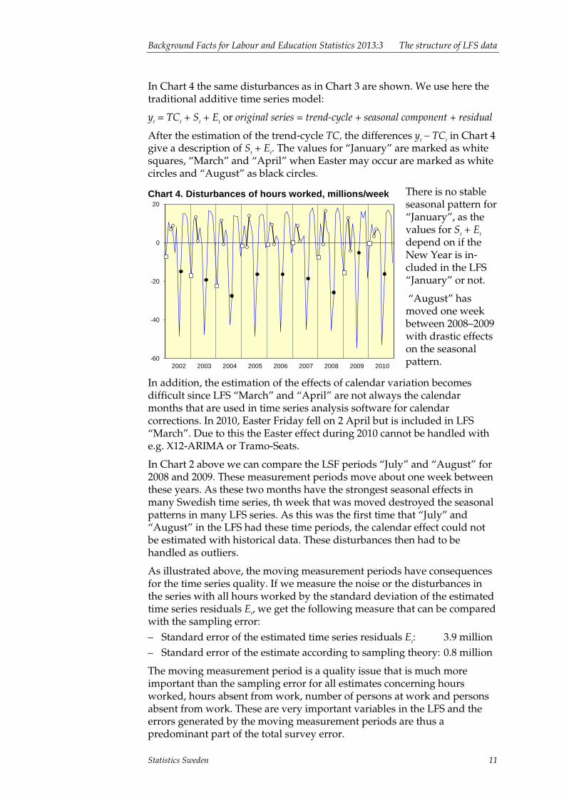
In Chart 4 the same disturbances as in Chart 3 are shown. We use here the traditional additive time series model:

yt = TCt + St + Et or original series = trend-cycle + seasonal component + residual

After the estimation of the trend-cycle TC, the differences yt – TCt in Chart 4 give a description of St + Et. The values for “January” are marked as white squares, “March” and “April” when Easter may occur are marked as white circles and “August” as black circles.

Chart 4. Disturbances of hours worked, millions/week

There is no stable seasonal pattern for “January”, as the values for St + Et depend on if the New Year is in-cluded in the LFS “January” or not.

“August” has moved one week between 2008–2009 with drastic effects on the seasonal pattern.

In addition, the estimation of the effects of calendar variation becomes difficult since LFS “March” and “April” are not always the calendar months that are used in time series analysis software for calendar corrections. In 2010, Easter Friday fell on 2 April but is included in LFS “March”. Due to this the Easter effect during 2010 cannot be handled with e.g. X12-ARIMA or Tramo-Seats.

In Chart 2 above we can compare the LSF periods “July” and “August” for 2008 and 2009. These measurement periods move about one week between these years. As these two months have the strongest seasonal effects in many Swedish time series, th week that was moved destroyed the seasonal patterns in many LFS series. As this was the first time that “July” and “August” in the LFS had these time periods, the calendar effect could not be estimated with historical data. These disturbances then had to be handled as outliers.

As illustrated above, the moving measurement periods have consequences for the time series quality. If we measure the noise or the disturbances in the series with all hours worked by the standard deviation of the estimated time series residuals Et, we get the following measure that can be compared with the sampling error: – Standard error of the estimated time series residuals Et: 3.9 million – Standard error of the estimate according to sampling theory: 0.8 million

The moving measurement period is a quality issue that is much more important than the sampling error for all estimates concerning hours worked, hours absent from work, number of persons at work and persons absent from work. These are very important variables in the LFS and the errors generated by the moving measurement periods are thus a predominant part of the total survey error.

-60

-40

-20

0

20

2002 2003 2004 2005 2006 2007 2008 2009 2010



Good correction methods must be developed to overcome these disturbances. Otherwise, the usability of the Labour Force Survey will be limited.

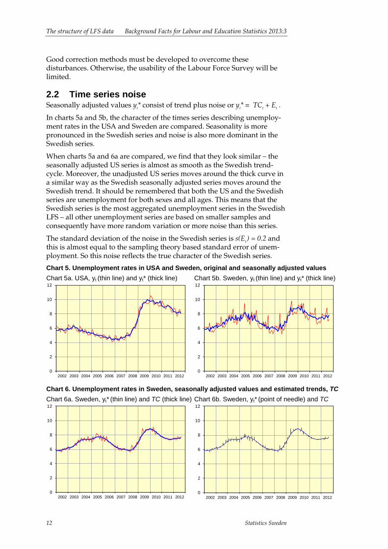
2.2 Time series noise Seasonally adjusted values yt* consist of trend plus noise or yt* = TCt + Et .

In charts 5a and 5b, the character of the times series describing unemploy-ment rates in the USA and Sweden are compared. Seasonality is more pronounced in the Swedish series and noise is also more dominant in the Swedish series.

When charts 5a and 6a are compared, we find that they look similar – the seasonally adjusted US series is almost as smooth as the Swedish trend-cycle. Moreover, the unadjusted US series moves around the thick curve in a similar way as the Swedish seasonally adjusted series moves around the Swedish trend. It should be remembered that both the US and the Swedish series are unemployment for both sexes and all ages. This means that the Swedish series is the most aggregated unemployment series in the Swedish LFS – all other unemployment series are based on smaller samples and consequently have more random variation or more noise than this series.

The standard deviation of the noise in the Swedish series is s(Et ) = 0.2 and this is almost equal to the sampling theory based standard error of unem-ployment. So this noise reflects the true character of the Swedish series.

Chart 5. Unemployment rates in USA and Sweden, original and seasonally adjusted values Chart 5a. USA, yt (thin line) and yt* (thick line)

Chart 5b. Sweden, yt (thin line) and yt* (thick line)

Chart 6. Unemployment rates in Sweden, seasonally adjusted values and estimated trends, TC Chart 6a. Sweden, yt* (thin line) and TC (thick line)

Chart 6b. Sweden, yt* (point of needle) and TC

0

2

4

6

8

10

12

2002 2003 2004 2005 2006 2007 2008 2009 2010 2011 20120

2

4

6

8

10

12

2002 2003 2004 2005 2006 2007 2008 2009 2010 2011 2012

0

2

4

6

8

10

12

2002 2003 2004 2005 2006 2007 2008 2009 2010 2011 20120

2

4

6

8

10

12

2002 2003 2004 2005 2006 2007 2008 2009 2010 2011 2012



We quote here the Quality Guidelines of Statistics Canada (2009):

12.1.2 Trend-cycle estimation Seasonal adjustment of highly volatile series may not be enough to draw conclusion on the current trend-cycle direction. In those cases, further smoothing of the seasonally adjusted series is advisable to eliminate most of the irregular component. The resulting trend-cycle estimate is to be considered auxiliary information to the seasonally adjusted series.

The conclusions that we draw from the comparisons between Swedish time series and corresponding series from the USA in charts 5 and 6 are of a general character. Monthly Swedish series have as a rule stronger seasonal variation and more noise (irregular component or residuals) than series from the USA. So according to Statistics Canada’s guidelines, further smoothing is practically always advisable with Swedish monthly series.

When the character of time series from small countries is different from time series from large countries such as the USA, the guidelines for time-series analysis should be different. According to our experience of Swedish time series, further smoothing, i.e. trend-cycle estimation is not only advisable but as a rule necessary – to measure rate of change we must use the estimated trend-cycle. And we do not consider the trend-cycle estimate as auxiliary information to the seasonally adjusted series; instead, we regard the seasonally adjusted series as auxiliary information to the estimated trend-cycle. First we judge the trend-cycle pattern TCt and then we look at the last yt* values. If the last seasonally adjusted values are above the estimated trend-cycle, this can be an indication of a turning point, e.g. that the trend-cycle could soon turn upwards.

As seasonally adjusted values yt* consist of trend-cycle plus noise (yt* = TCt + Et ), then the difference between the seasonally adjusted series and the estimated trend-cycle is the series of estimated residuals Et. As a rule, there is no interesting information in these residuals. The LFS is a sample survey and these time-series residuals in many cases only give a picture of the sampling errors. In the example above with the Swedish unemployment rate, the standard deviation of the noise was s(Et) = 0.2 and this was almost equal to the sampling theory-based standard error of the total unemployment rate. Our interpretation is that this noise reflects the sampling error for each month.

2.3 The effects of the panel design The Swedish Labour Force Survey uses a panel design where each panel is interviewed once every third month. Each person is interviewed a total of eight times. When we compare surveys for e.g. January and April or the first and second quarters of a specific year, seven-eighths of the two samples consist of identical persons.

The idea behind this panel design is that quarterly rates of change should have small standard errors. However, the autocorrelation functions of all time series will be a mixture of the true autocorrelations on the labour market and artificial autocorrelations created by the sample design.

These disturbing autocorrelations due to panel effects make the ARIMA-models complicated and much more difficult to identify and estimate. As we have a system with about 1 250 series, we must use automatic model



selections in Tramo-Seats or X12-Arima. Since the ARIMA-models are complicated, the chosen models will not be stable over time; when more data are added, different ARIMA-models may be chosen.

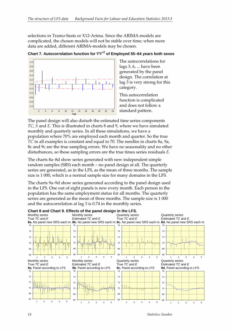
Chart 7. Autocorrelation function for ∇∇12 of Employed 55–64 years both sexes

The autocorrelations for lags 3, 6, ... have been generated by the panel design. The correlation at lag 3 is very strong for this category.

This autocorrelation function is complicated and does not follow a standard pattern.

The panel design will also disturb the estimated time series components TC, S and E. This is illustrated in charts 8 and 9, where we have simulated monthly and quarterly series. In all these simulations, we have a population where 70% are employed each month and quarter. So the true TC in all examples is constant and equal to 70. The needles in charts 8a, 9a, 8c and 9c are the true sampling errors. We have no seasonality and no other disturbances, so these sampling errors are the true times series residuals E.

The charts 8a–8d show series generated with new independent simple random samples (SRS) each month – no panel design at all. The quarterly series are generated, as in the LFS, as the mean of three months. The sample size is 1 000, which is a normal sample size for many domains in the LFS.

The charts 9a–9d show series generated according to the panel design used in the LFS. One out of eight panels is new every month. Each person in the population has the same employment status for all months. The quarterly series are generated as the mean of three months. The sample size is 1 000 and the autocorrelation at lag 3 is 0.74 in the monthly series.

Chart 8 and Chart 9. Effects of the panel design in the LFS. Monthly series True TC and E 8a. No panel new SRS each m.

Monthly series Estimated TC and E 8b. No panel new SRS each m.

Quarterly series True TC and E 8c. No panel new SRS each m.

Quarterly series Estimated TC and E 8d. No panel new SRS each m.

Monthly series True TC and E 9a. Panel according to LFS

Monthly series Estimated TC and E 9b. Panel according to LFS

Quarterly series True TC and E 9c. Panel according to LFS

Quarterly series Estimated TC and E 9d. Panel according to LFS

Lag24222018161412108642

1.0

0.8

0.6

0.4

0.2

0.0

-0.2

-0.4

-0.6

-0.8

-1.0

66

68

70

72

74

76

1 2 3 4 566

68

70

72

74

76

1 2 3 4 566

68

70

72

74

76

1 2 3 4 566

68

70

72

74

76

1 2 3 4 5

66

68

70

72

74

76

1 2 3 4 566

68

70

72

74

76

1 2 3 4 566

68

70

72

74

76

1 2 3 4 566

68

70

72

74

76

1 2 3 4 5



The trend-cycles in charts 8 and 9 have been estimated by applying moving averages similar to the filters in X12-ARIMA.

The problems with the panel design are clearly shown in charts 9c and 9d. Due to the panel design, the quarterly sampling errors are almost the same as during the previous quarter and these sampling errors are misinter-preted as a trend-cycle. The monthly series in charts 9a and 9b also have the same problem – nearly the same sampling errors come back after three months and this will distort the trend-cycle.

The estimated irregular component E also becomes distorted; in Chart 9d it looks as if there are almost no random disturbances. As most of the true E component is included in the estimated TC component, the estimated E component consists of values close to zero.

The charts 8a–8d show that even when the residuals are uncorrelated, the trend-cycle is estimated with errors due to the well-known Slutzky-Yule effect; a moving average of a random series oscillates. However, the errors are smaller than in cases where the residuals are positively autocorrelated.

In the charts below, the seasonally adjusted values y* are the points of the needles; the curve is the estimated trend-cycle TC; and the vertical lines, the needles, are the estimated time series residuals, E.

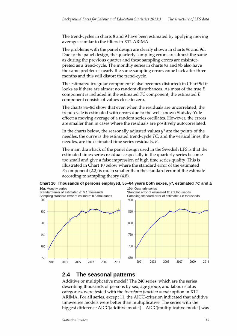
The main drawback of the panel design used in the Swedish LFS is that the estimated times series residuals especially in the quarterly series become too small and give a false impression of high time series quality. This is illustrated in Chart 10 below where the standard error of the estimated E-component (2.2) is much smaller than the standard error of the estimate according to sampling theory (4.8).

Chart 10. Thousands of persons employed, 55–64 years both sexes, y*, estimated TC and E 10a. Monthly series Standard error of estimated E: 5.1 thousands Sampling standard error of estimate: 8.5 thousands

10b. Quarterly series Standard error of estimated E: 2.2 thousands Sampling standard error of estimate: 4.8 thousands

2.4 The seasonal patterns Additive or multiplicative model? The 240 series, which are the series describing thousands of persons by sex, age group, and labour status categories, were tested with the transform function = auto option in X12-ARIMA. For all series, except 11, the AICC-criterion indicated that additive time-series models were better than multiplicative. The series with the biggest difference AICC(additive model) – AICC(multiplicative model) was

650

700

750

800

850

900

2001 2003 2005 2007 2009 2011 650

700

750

800

850

900

2001 2003 2005 2007 2009 2011



seasonally adjusted with both models. However, the estimated seasonal components are almost the same; this is illustrated in Chart 11 below. As the seasonal component in X12-ARIMA is adaptive, additive and multiplicative time series models can generate similar estimates. The estimated St component for the multiplicative model can be transformed into normal scale of 1000s persons by St = yt - yt*

Chart 11. Additive and multiplicative seasonal components are almost the same

We also analysed the series describing hours actually worked. Only one series of these was clearly multiplicative – hours worked within agriculture, forestry and fishing. In Chart 12a, we can see that variation is more than 2 million in the beginning of the series but only about 1 million at the end. After logarithmic transformation, the variation is about the same independent of the series level. The conclusion is that the series has multiplicative seasonal patterns. However, additive and multiplicative seasonal adjust-ments are equally good; the standard deviation of Et from additive adjustment is 0.22, and the corresponding standard deviation from the multiplicative adjustment is 0.23 when the multiplicative component is transformed into normal scale by Et = yt*- TCt.

Chart 12. Hours worked within agriculture forestry and fishing, normal and logarithmic scales 12a. Hours per week, millions

12b. Log10(Hours per week, millions)

2

4

6

8

10

87 89 91 93 95 97 99 01 03 05 07 09 11 0,4

0,5

0,6

0,7

0,8

0,9

1,0

87 89 91 93 95 97 99 01 03 05 07 09 11

Background Facts for Labour and Education Statistics 2013:3 How to achieve consistency


3 How to achieve consistency The structure of LFS data must be taken into account when systems are developed for seasonal adjustment. The additivity necessary for consistency between different series is determined by the multi-dimensional frequency tables that are generated by the Labour Force Survey. The moving measure-ment period will disturb series describing persons at work or absent, hours worked or absent, but not the series describing stable states as employed or unemployed. The time series noise makes trend-cycle estimates important and the panel design will generate artificial autocorrelations at lag 3 in monthly series. When these autocorrelations are strong, the sampling errors will be misinterpreted as trend-cycle, and it may be risky to use ARIMA-models for estimation of seasonality and trend as in Tramo-Seats. The fact that additive time series models can be used for LFS data will simplify the work of deriving consistent seasonally adjusted values.

3.1 Different methods to achieve consistency The monthly and quarterly time series generated by the LFS are consistent before seasonal adjustments are made. This means that series for sums of categories agree with the sums of their parts. But after outlier corrections and seasonal adjustment, the adjusted values are as a rule no longer consistent.

Many statisticians prefer the direct method for seasonal adjustment, where each series is adjusted as best as possible without regards to other series. The sum and the parts are inconsistent, but that is considered a natural consequence of the fact that statistical estimation never can be perfect.

The users often want consistency between a seasonally adjusted sum and the sum of the seasonally adjusted parts. As a rule, they use the indirect method where the parts are seasonally adjusted and the sum of the seasonally adjusted parts is used as the seasonally adjusted sum. Due to the fact that the sum now has not necessarily been adjusted in the best possible way, many statisticians do not want to use the indirect method. E.g. in ESS Guidelines on Seasonal Adjustment (Eurostat 2009), the direct method is recommended except when the parts have significantly different seasonal patterns.

Both the direct and the indirect methods have the disadvantage that all information is not used. In the direct method the information regarding the additivity conditions is not used; in the indirect method the information in the aggregated series is not used despite the fact that the aggregated series as a rule have better time series quality, as the time series noise is less disturbing due to relatively smaller sampling errors.

According to the ESS Guidelines (op. cit.), it is acceptable to use the direct method and adjust the seasonally adjusted values to achieve consistency, if there are strong user requirements for consistency. A method for this has been developed by Stuckey, Zhang and McLaren (2004). Their method has been tested and implemented for use in the Swedish quarterly National Accounts. This work is reported in Elezovic, Odencrants and Xie (2009).

How to achieve consistency Background Facts for Labour and Education Statistics 2013:3


3.2 Preconditions A reference group with experienced analysts from the central government was formed for the work in developing a system for consistent seasonal adjustment. If each time series is counted as four – e.g. persons employed monthly, employment rates monthly, persons employed quarterly and employment rates quarterly, the reference group wanted about 5 000–6 000 series to be seasonally adjusted. The total number of published series that can be seasonally adjusted is about 30 000 including both monthly and quarterly series. This shows the importance of the LFS in Sweden – it is used by many analysts, and different users need different series so that the total number of important series is large.

We defined the following preconditions for our work with the system for time series analysis:

1. About 4 000 series should be included in the system. These series describe labour status category by sex and age group, subdivisions of labour status category by sex and age group, and hours worked by sex, degree of attachment to the labour force and kind of economic activity. The structure of LFS data will be regarded when designing the system.

2. Seasonally adjusted values and estimated trend-cycle values should be consistent in three dimensions: sex, age group, and labour status category; i.e. employed, unemployed, not in labour force. Seasonally adjusted series for number of persons and corresponding per cent of population should be consistent. Seasonally adjusted monthly series and corresponding quarterly series should also be consistent. Pre-treatment as adjustments for trading day, moving holiday and moving measurement period should be consistent. Outlier corrections should also be consistent. Different seasonally adjusted series for hours worked should be consistent in a similar way.

3. Adjustments to attain consistency should be as small as possible. Real data should not be subject to unnecessary corrections and adjustments.

4. Subject matter competence should be used when deciding if a value is an outlier or an indication of a real rapid change.

5. The system will be handled by a small number of persons working under pressure. These persons are not specialised time series analysts; they belong to the ordinary subject matter staff who are responsible for the LFS. Risks for mistakes should be eliminated as much as possible. Robust methods should therefore be chosen.

3.3 Choice of method As we mentioned in Section 3.2, both the indirect and direct methods do not use all available information. If this information is used in the estimation of time series components, it should be possible to improve the quality of these estimates. It is this methodological challenge together with strong user demands for consistency in a system with about 4 000 time series that have induced us to work with developing a system for consistent seasonal adjustment.

How to fulfil precondition 2 above regarding consistency? Consistent seasonal adjustment in a three-way frequency table can be achieved in different ways.



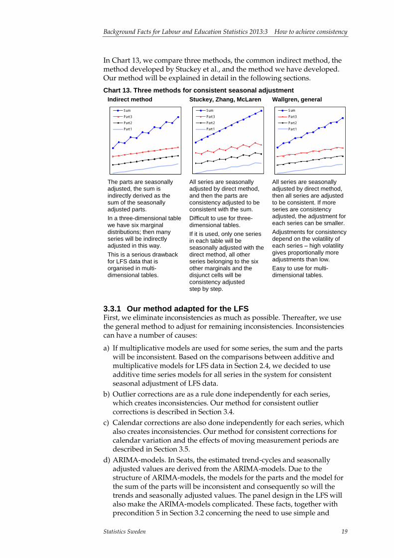
In Chart 13, we compare three methods, the common indirect method, the method developed by Stuckey et al., and the method we have developed. Our method will be explained in detail in the following sections.

Chart 13. Three methods for consistent seasonal adjustment Indirect method

The parts are seasonally adjusted, the sum is indirectly derived as the sum of the seasonally adjusted parts. In a three-dimensional table we have six marginal distributions; then many series will be indirectly adjusted in this way. This is a serious drawback for LFS data that is organised in multi-dimensional tables.

Stuckey, Zhang, McLaren

All series are seasonally adjusted by direct method, and then the parts are consistency adjusted to be consistent with the sum. Difficult to use for three-dimensional tables. If it is used, only one series in each table will be seasonally adjusted with the direct method, all other series belonging to the six other marginals and the disjunct cells will be consistency adjusted step by step.

Wallgren, general

All series are seasonally adjusted by direct method, then all series are adjusted to be consistent. If more series are consistency adjusted, the adjustment for each series can be smaller. Adjustments for consistency depend on the volatility of each series – high volatility gives proportionally more adjustments than low. Easy to use for multi-dimensional tables.

3.3.1 Our method adapted for the LFS First, we eliminate inconsistencies as much as possible. Thereafter, we use the general method to adjust for remaining inconsistencies. Inconsistencies can have a number of causes:

a) If multiplicative models are used for some series, the sum and the parts will be inconsistent. Based on the comparisons between additive and multiplicative models for LFS data in Section 2.4, we decided to use additive time series models for all series in the system for consistent seasonal adjustment of LFS data.

b) Outlier corrections are as a rule done independently for each series, which creates inconsistencies. Our method for consistent outlier corrections is described in Section 3.4.

c) Calendar corrections are also done independently for each series, which also creates inconsistencies. Our method for consistent corrections for calendar variation and the effects of moving measurement periods are described in Section 3.5.

d) ARIMA-models. In Seats, the estimated trend-cycles and seasonally adjusted values are derived from the ARIMA-models. Due to the structure of ARIMA-models, the models for the parts and the model for the sum of the parts will be inconsistent and consequently so will the trends and seasonally adjusted values. The panel design in the LFS will also make the ARIMA-models complicated. These facts, together with precondition 5 in Section 3.2 concerning the need to use simple and

SumPart 3Part 2Part 1





robust methods, led us to decide to use X12-ARIMA in the system for consistent seasonal adjustments of LFS data.

e) ARIMA extrapolations. In X12-ARIMA, seasonally adjusted values and estimated trend-cycles for the last part of the series are based on ARIMA extrapolations. As these extrapolations are done with ARIMA-models, the extrapolations will be inconsistent – a sum and its parts will as a rule not agree. The ARIMA extrapolations are made consistent with the method based on a linear model for the frequency table generating the system of time series.

f) Trend and seasonal filters. In X12-ARIMA different moving average filters can be used for estimates of seasonally adjusted values and for the trend-cycle estimates. We decided to use the same trend and seasonal filters for all series whereby no inconsistencies are created. We prefer the 23-point Henderson trend filter and the s3x5 seasonal filter due to the strong volatility in Swedish series.

3.3.2 Combining estimates In the tables published by the LFS, there are several examples where there are many estimates of the same parameter. E.g. the seasonally adjusted total number of unemployed is estimated directly, but can also be obtained as the sum of seasonally unemployed men and unemployed women. These three estimated seasonally adjusted values are as a rule inconsistent.

How can several estimates that perhaps are inconsistent be combined into one estimate with better quality? This is a standard example in a course in statistical theory:

Assume that we have two independent estimators y1 and y2 of the parameter θ with variances 𝜎12 and 𝜎22. How can we combine these estimators in an optimal way?

The answer is the estimator 𝜃� = 𝜎22 /(𝜎12 + 𝜎22) · y1 + 𝜎12/(𝜎12 + 𝜎22) · y2 .

The variance of 𝜃� is smaller than both 𝜎12 and 𝜎22. So instead of two inconsistent estimates of the same parameter, we arrive at one estimate with better quality. We get the same estimator of the parameter that we now denote with β, by using a regression model:

yi = β · xi + εi where xi = 1 and the weights 1/ 𝜎𝑖2 are used for i = 1, 2.

3.3.3 Combining estimates in a one-way frequency table Assume that we have the one-way frequency table below with inconsistent values regarding one specific month in column (1). These values can either be seasonally adjusted values, estimated trend-cycle values or ARIMA extrapolated values to be used in X12-ARIMA for estimation at the endpoint of the series. As the number of employed both sexes should be employed men + employed women, all three cells in column (1) could be derived if the two parameters β1 and β2 were known.

Sex Employed, 1000s inconsistent values

yi (1)

Variance for the residuals in the ARIMA-model

(2)

Regression model

(3)

Employed, 1000s consistency adjusted

ŷi (4)

Men 2 300 320 β1 · 1 + β2 · 0 2 322 Women 2 100 310 β1 · 0 + β2 · 1 2 121 Both sexes 4 500 830 β1 · 1 + β2 · 1 4 443



How can the three observed values yi be used to estimate the two parameters β1 and β2? In the same way as we used regressions analysis in the example in Section 3.3.2, we can derive the consistent values 𝑦� in column (4). The model in column (3) has two dummy variables for men and women respectively:

yi = β1 · x1 + β2 · x2 + εi

We also use weights here and these weights are inversely proportional to the variance of the three series ARIMA-residuals in column (2). Volatile series will receive low weights and non-volatile series will get heavy weights.

3.3.4 Combining estimates in multidimensional tables Assume that we have the following two-dimensional frequency table with inconsistent ARIMA extrapolated values for a specific month. In this table we have neither consistency, so that:

Both sexes = Men + Women nor consistency so that:

Labour force = Employed + Unemployed nor consistency so that:

Population = Labour force + Not in labour force

Inconsistent table, 1000s of persons Employed Unemployed Not in labour

force Labour force Population

Men 2 300 60 450 2 400 2 700 Women 2 100 50 500 2 200 2 600 Both sexes 4 500 100 900 4 700 5 200

We can also use the method here that uses weighed regressions analysis, where the weights are inversely proportional to the variance of the ARIMA-residuals for each series.

Variances, ARIMA-residuals Employed Unemployed Not in labour


Men 320 100 250 248 0.43 Women 310 85 275 279 0.46 Both sexes 830 230 685 691 1.25

The regression model will have six x-variables, one dummy variable for each of the six disjunct cells (shaded) in the table below. The fifteen y-variables are in the 5x3 way table above with inconsistent values.

Regression model Employed Unemployed Not in

labour force Labour force Population

Men β1 β2 β3 β1 + β2 β1 + β2 + β3 Women β4 β5 β6 β4 + β5 β4 + β5 + β6 Both sexes β1 + β4 β2 + β5 β3 + β6 β1+β2+β4+β5 β1+β2+β3+β4+β5+β6

With weighed regression analysis we obtain the following frequency table that is consistent in two dimensions:

Consistent table, 1000s of persons Employed Unemployed Not in labour


Men 2 299.0 50.6 350.4 2 349.6 2 700.0 Women 2 119.7 47.7 432.6 2 167.4 2 600.0 Both sexes 4 418.7 98.3 783.0 4 517.0 5 300.0



The regression analysis used to obtain the table with consistent estimates is described in the table below. The design matrix is the matrix with the six dummy variables that describes the structure of the time series defined by the two-dimensional frequency table.

Regression analysis

Design matrix

y x1 x2 x3 x4 x5 x6 s2 weight = 1 / s2 𝒚� 2 300 1 0 0 0 0 0 320.00 0.00313 2299.0

60 0 1 0 0 0 0 100.00 0.01000 50.6 450 0 0 1 0 0 0 250.00 0.00400 350.4

2 400 1 1 0 0 0 0 248.00 0.00403 2349.6 2 700 1 1 1 0 0 0 0.43 100.00000 2700.0 2 100 0 0 0 1 0 0 310.00 0.00323 2119.7

50 0 0 0 0 1 0 85.00 0.01176 47.7 500 0 0 0 0 0 1 275.00 0.00364 432.6

2 200 0 0 0 1 1 0 279.00 0.00358 2167.4 2 600 0 0 0 1 1 1 0.46 100.00000 2600.0 4 500 1 0 0 1 0 0 830.00 0.00120 4418.7

100 0 1 0 0 1 0 230.00 0.00435 98.3 900 0 0 1 0 0 1 685.00 0.00146 783.0

4 700 1 1 0 1 1 0 691.00 0.00145 4517.0 5300 1 1 1 1 1 1 1.25 100.00000 5300.0

The three population values have intentionally obtained heavy weights of 100. In this way, the population values that are defined by the population register and used as the frame for the LFS are kept constant.

With this kind of linear model, we have adjusted the outlier corrections, the calendar and moving “months” corrections and the ARIMA-extrapolations used by X12-ARIMA. In this way, all input series to the seasonal adjustment in X12-ARIMA become consistent. Since the same filters are used for all series the output from X12-ARIMA is also consistent.

3.3.5 Our method for seasonal adjustment of LFS data A k-way frequency table is additive in k dimensions. These additivity conditions can be expressed with a linear model as explained in Section 3.3.4. We will use linear models of this kind to adjust estimates that are not additive, but should be additive. We thereby improve the quality of the estimates by using auxiliary information on the additivity of the underlying parameters.

Let us use Module 1, the first times series analysis module we designed, to illustrate our general method. This module uses data from a three dimensional frequency table with persons by age, sex and labour status category. Sixteen age groups, three sex groups and five labour status categories are used. In all, 16 · 3 · 5 = 240 series are the input into the module according to the categories below:

15-19 15-24 16-19 16-24 18-24 20-24 25-34 35-44 45-54 55-59 60-64 55-64 16-64 18-64 65-74 15-74 .

Men Women Both sexes .

Employed Unemployed Not in labour force In labour force Population

Out of these series only 10 · 2 · 3 = 60 series are from disjunct cells, the others are combinations of these:

15 16-17 18-19 20-24 25-34 35-44 45-54 55-59 60-64 65-74

Men Women .

Employed Unemployed Not in labour force



If these 240 time series are analysed with X12-ARIMA, we may obtain 240 estimated seasonal components for a specific month, or we may obtain 240 estimated outlier effects for a specific month, or we may obtain 240 ARIMA extrapolations for a month in the future. These seasonal components, outlier effects or extrapolations can be inconsistent – the additivity conditions that the original time series values follow will as a rule not hold when each series is analysed independently from the other series.

Each month, we obtain 240 estimates defined by 60 parameters in this way. How should these 240 estimates be used to obtain the best estimates of the 60 parameters? The idea is to combine the information in all 240 series. The indirect method for seasonal adjustment would use only the information in the 60 disjunct series and the remaining 240 – 60 = 180 series would have been derived indirectly as sums of different combinations of the 60 disjunct series. So the indirect method will discard the information in the majority of the series in the system. The discarded information should also have better quality than the 60 series used, as the 180 series that are discarded are on a more aggregate level and have smaller coefficients of variation.

We define the vector y as the vector with the 240 values for a specific month that may be inconsistent. The vector β is the vector of 60 unknown parameters for the disjunct cells, and the design matrix X is the matrix of dummy variables that defines how each of the 240 values are derived from the 60 disjunct values. The vector 𝐲� is the vector of 240 consistent values and these values are obtained from the regression analysis. As weights in the regression analyses, we use 1/s2 where s2 is the variance of the ARIMA residuals for each series.

It should be noted that with the method we use for LFS data, we only adjust outlier corrections, calendar and moving “month” corrections, and the extrapolated ARIMA values. When we have eliminated these inconsistencies, we can use the seasonally adjusted values and estimated trend-cycle values from X12-ARIMA exactly as they are without adjustments.

The method is also flexible and easy to use. After Module 1, the first time series analysis module we designed, had been used for publishing seasonally adjusted LFS data, we developed Module 2 where subdivisions of the labour status categories from Module 1 are analysed. All 960 series with persons by detailed labour status categories, age class and sex are seasonally adjusted in Module 2. For the subdivision of employed persons we use the outlier corrections and ARIMA-extrapolations from Module 1. And the values from Module 1 are not altered – they are given very heavy weights in the regression analysis so that they remain unchanged in the same way that the population values in Section 3.3.4 were kept fixed. This makes it easy to obtain consistency between the 240 series in Module 1 and the 960 series in Module 2.

In this way we have obtained consistent seasonally adjusted values and trends for 240 + (960 - 240) = 960 series regarding persons by labour status category, age and sex.

After that, we obtain 960 consistent series by division with population values regarding per cent of population (or labour force for unemployment rate).



By taking the averages of the three months belonging to the same quarter, we also obtain 960 consistent quarterly series regarding persons by labour status category, age and sex. And finally, by division with population values, we obtain 960 consistent quarterly series regarding per cent of the population or the labour force.

The methods used to go from 960 series on number of persons monthly, to 4 · 960 series regarding number of persons, per cent and both monthly and quarterly series, consist of simple computations, which make the risk of errors small.

3.4 Consistent ARIMA-outlier corrections After comparing output for independent X12-ARIMA runs for many LSF series, we found that the outlier corrections generate many inconsistencies. In this section we describe our method for consistent outlier correction in a system of time series defined by a multidimensional frequency table.

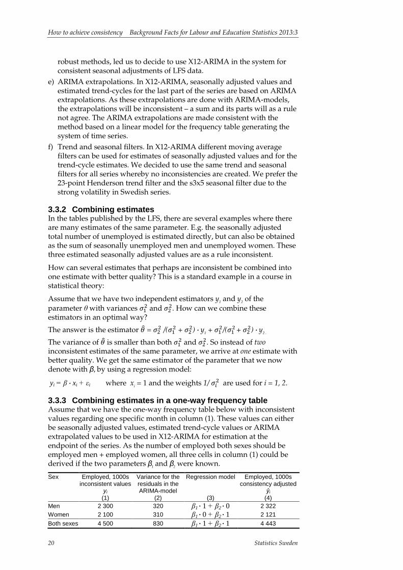
3.4.1 Outlier detection in time series from frequency tables There are options for automatic outlier detection and correction in both X12-ARIMA and Tramo. For each time series, the software searches for extreme ARIMA-residuals and tests for different kinds of outliers by including appropriate regression variables in the model. We illustrate our method with the following system of 12 quarterly time series:

Chart 14. Persons by sex and labour status category, 1000s 2nd quarter 1992 Men Women Both sexes Employed 2 199.8 2 080.3 4 280.1 Unemployed 135.7 77.0 212.7 Not in labour force 429.7 523.0 952.7 Population 2 765.2 2 680.3 5 445.5

In this table there are six disjunct cells and two marginal distributions that define the system of times series and the additivity conditions. The system consists of nine LFS time series and three population series, where the population series are smooth and therefore are not seasonally adjusted.

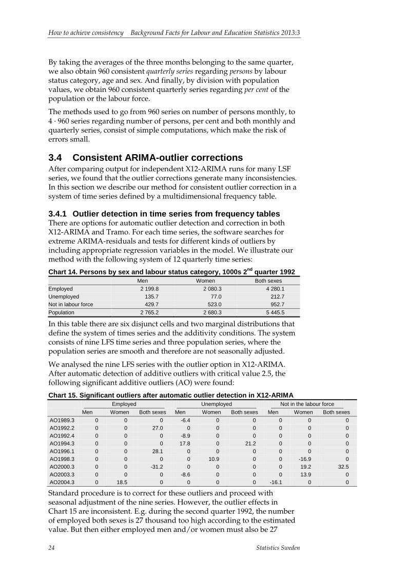
We analysed the nine LFS series with the outlier option in X12-ARIMA. After automatic detection of additive outliers with critical value 2.5, the following significant additive outliers (AO) were found:

Chart 15. Significant outliers after automatic outlier detection in X12-ARIMA Employed Unemployed Not in the labour force

Men Women Both sexes Men Women Both sexes Men Women Both sexes AO1989.3 0 0 0 -6.4 0 0 0 0 0 AO1992.2 0 0 27.0 0 0 0 0 0 0 AO1992.4 0 0 0 -8.9 0 0 0 0 0 AO1994.3 0 0 0 17.8 0 21.2 0 0 0 AO1996.1 0 0 28.1 0 0 0 0 0 0 AO1998.3 0 0 0 0 10.9 0 0 -16.9 0 AO2000.3 0 0 -31.2 0 0 0 0 19.2 32.5 AO2003.3 0 0 0 -8.6 0 0 0 13.9 0 AO2004.3 0 18.5 0 0 0 0 -16.1 0 0

Standard procedure is to correct for these outliers and proceed with seasonal adjustment of the nine series. However, the outlier effects in Chart 15 are inconsistent. E.g. during the second quarter 1992, the number of employed both sexes is 27 thousand too high according to the estimated value. But then either employed men and/or women must also be 27



thousand higher than expected and the categories unemployed and/or not in the labour force must be 27 thousand lower than expected.

The next step is therefore to estimate all effects for the quarters in question. With one exception (men not in the labour force 2004 Q3), the outlier effects from Chart 15 remain in Chart 16 but now we have estimates for all series.

Chart 16. Estimation of all outlier effects for the quarters with significant outliers * =significant with critical value 2.5

Employed Unemployed Not in the labour force Men Women Both sexes Men Women Both sexes Men Women Both sexes

AO1989.3 -4.4 3.4 -2.5 -6.1* -8.4* -12.5* 8.5 5.2 10.1 AO1992.2 12.3* 13.5* 25.9* -0.4 -4.8 -5.5 -11.8* -9.4 -21.5* AO1992.4 8.3 2.0 11.1 -8.5* -1.5 -7.5 2.8 2.8 4.6 AO1994.3 1.7 -4.4 -1.8 17.2* 5.8 22.2* -16.6* -0.5 -18.7* AO1996.1 15.9* 11.4* 27.6* -2.6 -0.2 -4.3 -11.7* -9.2* -23.4* AO1998.3 4.5 5.7 11.9 2.0 12.1* 12.5* -7.0 -19.2* -22.8* AO2000.3 -16.0* -12.4* -28.2* 2.1 -2.7 0.4 13.0* 18.9* 30.4* AO2003.3 4.6 -4.3 -1.2 -8.7* -0.1 -8.9 3.9 11.8* 15.5 AO2004.3 2.2 14.8* 15.3 -2.0 -0.5 -3.4 -0.2 -5.9 -7.6

The estimated outlier effects in Chart 16 above are not consistent. E.g. for 1989 Q3, the effects for employed men + employed women are not equal to both sexes (-4.4 + 3.4 ≠ -2.5) and the three effects for men do not sum to zero (-4.4 -6.1 + 8.5 ≠ 0). As the population of men should not be adjusted, this sum should be zero.

Using the methods described in the previous sections, the inconsistent estimates in Chart 16 can be improved if the information in the additivity conditions is used as auxiliary information. After this improvement, we obtain the new estimated outlier effects in Chart 17 that are consistent.

Chart 17. Consistent estimates of all outlier effects for the quarters with significant outliers Employed Unemployed Not in the labour force

Men Women Both sexes Men Women Both sexes Men Women Both sexes AO1989.3 -3.5 3.1 -0.4 -5.4 -7.7 -13.1 8.9 4.6 13.5 AO1992.2 12.3 13.9 26.2 -0.5 -4.7 -5.2 -11.9 -9.1 -21.0 AO1992.4 7.2 0.3 7.5 -8.3 -1.5 -9.8 1.1 1.1 2.2 AO1994.3 1.0 -4.5 -3.4 16.8 5.4 22.2 -17.9 -0.9 -18.8 AO1996.1 15.6 11.0 26.6 -3.0 -0.9 -3.9 -12.6 -10.0 -22.7 AO1998.3 4.7 6.5 11.2 1.6 11.7 13.4 -6.4 -18.2 -24.6 AO2000.3 -15.5 -14.1 -29.6 2.5 -3.1 -0.6 13.0 17.2 30.2 AO2003.3 4.6 -7.7 -3.1 -8.5 -1.5 -10.0 4.0 9.2 13.1 AO2004.3 2.2 11.2 13.4 -1.9 -2.3 -4.1 -0.3 -8.9 -9.2

The regression analysis is described in Chart 18. In the first column with numbers in Chart 18, the inconsistent estimated outlier effects from X12-ARIMA are given. The second column contains the standard deviations of the estimated outlier effects. These standard deviations are used for the weights in the regressions analysis. In the last column, we have the fitted values from the regression analysis that are the final consistent estimates of the outlier effects.

Note that we have added three rows with zeros as outlier effects for the series with the three populations that have very small standard errors (arbitrarily set to 0.1 by us). In this way we use the auxiliary information that

employed + unemployed + persons not in the labour force = the population



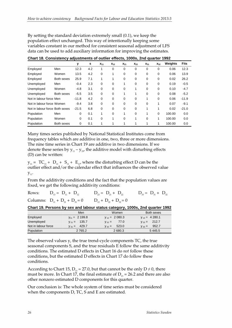
By setting the standard deviation extremely small (0.1), we keep the population effect unchanged. This way of intentionally keeping some variables constant in our method for consistent seasonal adjustment of LFS data can be used to add auxiliary information for improving the estimates.

Chart 18. Consistency adjustments of outlier effects, 1000s, 2nd quarter 1992

y s x11 x12 x21 x22 x31 x32 Weights Fits

Employed Men 12.3 4.2 1 0 0 0 0 0 0.06 12.3 Employed Women 13.5 4.2 0 1 0 0 0 0 0.06 13.9 Employed Both sexes 25.9 7.1 1 1 0 0 0 0 0.02 26.2 Unemployed Men -0.4 2.3 0 0 1 0 0 0 0.19 -0.5 Unemployed Women -4.8 3.1 0 0 0 1 0 0 0.10 -4.7 Unemployed Both sexes -5.5 3.5 0 0 1 1 0 0 0.08 -5.2 Not in labour force Men -11.8 4.2 0 0 0 0 1 0 0.06 -11.9 Not in labour force Women -9.4 3.8 0 0 0 0 0 1 0.07 -9.1 Not in labour force Both sexes -21.5 6.8 0 0 0 0 1 1 0.02 -21.0 Population Men 0 0.1 1 0 1 0 1 0 100.00 0.0 Population Women 0 0.1 0 1 0 1 0 1 100.00 0.0 Population Both sexes 0 0.1 1 1 1 1 1 1 100.00 0.0

Many times series published by National Statistical Institutes come from frequency tables which are additive in one, two, three or more dimensions. The nine time series in Chart 19 are additive in two dimensions. If we denote these series by y11 – y33, the additive model with disturbing effects (D) can be written:

y11 = TC11 + D11 + S11 + E11, where the disturbing effect D can be the outlier effect and/or the calendar effect that influences the observed value y11.

From the additivity conditions and the fact that the population values are fixed, we get the following additivity conditions:

Rows: D13 = D11 + D12 D23 = D21 + D22 D33 = D31 + D32

Columns: D11 + D21 + D31 = 0 D12 + D22 + D32 = 0

Chart 19. Persons by sex and labour status category, 1000s, 2nd quarter 1992 Men Women Both sexes Employed y11 = 2 199.8 y 12 = 2 080.3 y 13 = 4 280.1 Unemployed y 21 = 135.7 y 22 = 77.0 y 23 = 212.7 Not in labour force y 31 = 429.7 y 32 = 523.0 y 33 = 952.7 Population 2 765.2 2 680.3 5 445.5

The observed values y, the true trend-cycle components TC, the true seasonal components S, and the true residuals E follow the same additivity conditions. The estimated D effects in Chart 16 do not follow these conditions, but the estimated D effects in Chart 17 do follow these conditions.

According to Chart 15, D13 = 27.0, but that cannot be the only D ≠ 0, there must be more. In Chart 17, the final estimate of D13 = 26.2 and there are also other nonzero estimated D components for this quarter.

Our conclusion is: The whole system of time series must be considered when the components D, TC, S and E are estimated.



3.4.2 Outlier corrections in Module 1 In this section we show some output from Module 1 with data up to June 2009 and July 2009. After updating the data files, the first output shows the result from a test of the consistency of all variables that have been updated with values for June 2009. The regression residuals where the consistency is tested have the following minimum and maximum. As all residuals are almost zero, this shows that input was consistent. Variable: N Minimum Maximum Regression residuals 240 -0.000602 0.000749 measured in 1000s of persons The first use of X12-ARIMA is an analysis where the standardised ARIMA-residuals of all input series are plotted. The plot with standardised residuals for June 2009 shows that all 240 input series look normal – there are no signs of outliers during this month. As a rule, these residual plots are similar to this plot.

June 2009:

The same kind of plot for July 2009 shows that many input series have standardised ARIMA-residuals that are extreme. It was decided that July 2009 was a month that required outlier corrections. The outlier effects for all series during July 2009 were estimated as in charts 16–17 in Section 3.4.

July 2009:

The outlier effects were large for young persons employed and not in the labour force. The charts below describe both sexes 15–19 years, 2001–2012.

Employment rate, % Not in labour force rate, %

3.62.41.20.0-1.2-2.4-3.6

3.62.41.20.0-1.2-2.4-3.6

0

5

10

15

20

25

30

35

01 02 03 04 05 06 07 08 09 10 11 12 55

60

65

70

75

01 02 03 04 05 06 07 08 09 10 11 12



Traditionally we think of one series at a time when we search for outliers. Each month we ask: Is the last value in this series an outlier or not? If the answer is yes, we correct the last value.

But when we have LFS data from frequency tables, we cannot think of one outlier in one cell in the table only – there must be a number of cells in the table for a specific month that are parts of the same outlier effect. That is why we show ARIMA residuals for all series in the system in the residual plots above. So the question with LFS data should be: Are there outlier effects in the system of series this month or not? If the answer is yes, we correct all values in the system for the last month. So there is only one decision every month for the system of 240 series, not 240 independent decisions.

This means that automatic outlier corrections should not be used; instead, those responsible for the LFS make one decision every month for the whole system. This decision should be based on the plot of ARIMA residuals above and knowledge of the labour market and the data collection process. If the residual plot shows extreme residuals: – Are there labour market interventions or a strike this month? These

effects should be modelled with Tramo or REGARIMA in X12. This interesting outlier effect should be reported to the public.

– How did the data collection process work this month? This should be modelled as an uninteresting outlier.

– Are we expecting a turning point on the labour market? This should not be modelled as an outlier.

3.4.3 Seasonal outliers in X11 In X12-ARIMA there are two kinds of outlier corrections that can be used. First, there is the ARIMA-residual based outlier option that we have used in the previous sections. This option is exactly the same that is used in Tramo, and that is the only outlier option in the Tramo-Seats software.

There is another option in X12-ARIMA that was introduced in the early versions of X11. This option is based on the irregular component Et that is estimated in the X11 command of X12-ARIMA. In Section 3.4, we analyse a system of 12 time series, nine LFS series and three population series. Out of 72 quarterly values for these nine series, 34 quarters have no seasonal outliers and 38 quarters have seasonal outliers according to this outlier option in the X11 command. The outlier effects for these 38 quarters are inconsistent in the same way as in Chart 15 in Section 3.4.1. As a consequence, the seasonally adjusted values will also be inconsistent.

We have a system of 240 series in Module 1, and the outlier option in the X11 command will give us inconsistent outlier effects for most months. Our conclusion is that if you want consistent seasonal adjustment of LFS data, this outlier option in the X11 command cannot be used. Because this would lead to that almost all the data used would become artificial outlier corrected data instead of real LFS data.

3.5 Calendar variation and moving “months” In Section 2.1, we mention the problems that arise because the measure-ment periods in the LFS are moving. LFS “January” can start anywhere between 29 December and 4 January. Consequently, New Year vacations



are sometimes included and sometimes not included in the measurement period that is called “January” in the LFS. The seasonal pattern will differ depending on this. Swedish LFS data have very strong seasonality due to the long summer vacations that usually take place during July. If the measurement period that is called “July” moves and starts somewhere between 28 June and 6 July, this strong seasonal pattern will be disturbed. In Chart 2 in Section 2.1, the moving “months” in the LFS are shown.

Another consequence of these moving months is that the options for calendar corrections in standard software for seasonal adjustment are not suitable for LFS data. The number of Mondays, etc., that are used for calendar corrections are the number of Mondays in the calendar months, not the LFS measurement periods. The variables describing Easter are also not suitable for LFS data for the same reason.

Summing up: We have strong calendar variation and strong variation due to moving measurement periods in the LFS. Standard software for seasonal adjustment and calendar corrections are not adopted for LFS data. This means that methods suitable for the kind of time series that the LFS generates have been lacking.

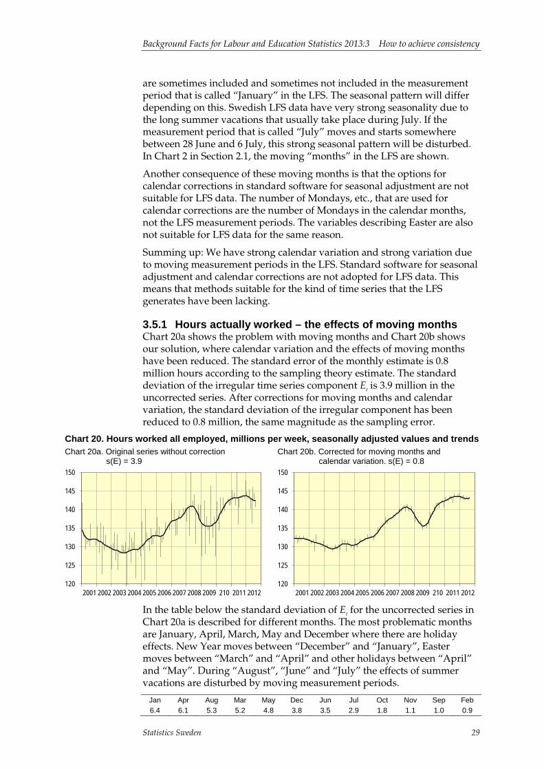
3.5.1 Hours actually worked – the effects of moving months Chart 20a shows the problem with moving months and Chart 20b shows our solution, where calendar variation and the effects of moving months have been reduced. The standard error of the monthly estimate is 0.8 million hours according to the sampling theory estimate. The standard deviation of the irregular time series component Et is 3.9 million in the uncorrected series. After corrections for moving months and calendar variation, the standard deviation of the irregular component has been reduced to 0.8 million, the same magnitude as the sampling error.

Chart 20. Hours worked all employed, millions per week, seasonally adjusted values and trends Chart 20a. Original series without correction s(E) = 3.9

Chart 20b. Corrected for moving months and calendar variation. s(E) = 0.8

In the table below the standard deviation of Et for the uncorrected series in Chart 20a is described for different months. The most problematic months are January, April, March, May and December where there are holiday effects. New Year moves between “December” and “January”, Easter moves between “March” and “April” and other holidays between “April” and “May”. During “August”, “June” and “July” the effects of summer vacations are disturbed by moving measurement periods.

Jan Apr Aug Mar May Dec Jun Jul Oct Nov Sep Feb 6.4 6.1 5.3 5.2 4.8 3.8 3.5 2.9 1.8 1.1 1.0 0.9

120

125

130

135

140

145

150

2001 2002 2003 2004 2005 2006 2007 2008 2009 210 2011 2012 120

125

130

135

140

145

150

2001 2002 2003 2004 2005 2006 2007 2008 2009 210 2011 2012



3.5.2 Our correction method The moving month effect can be handled with an extra question in the LFS interview. In the Swedish LFS, this extra question is included and the hours worked are split between months for measurement weeks that belong to two months. The Swedish National Accounts obtain this data on hours worked by industry and calendar months. These data are, however, not consistent with other LFS variables; this is discussed in Statistics Sweden (2012).

We have developed another method that uses information on reasons for being absent from work. The effects of Christmas, New Year, Easter and the other Easter related holidays during the spring are measured in the LFS interview. In addition, the effects of moving measurement periods have consequences for being absent from work for some reasons.

In Chart 21a, it can be seen that vacations during August 2009 (one of the four black boxes) were low due to a moving month effect. The LFS “August” was moved from a start at 28 July during 2008 to 3 August during 2009 and as a consequence hours absent went down. In Chart 21d the correction necessary has been estimated to be approximately 14 million hours.

In Chart 21a and 21b, we can see the effects of moving December and January. LFS “January” 2009 started 29 December 2008 and LFS “December” 2009 ended 3 January 2010. Both hours absent due to vacations and due to flexitime increased as the effect of absence for New Year celebrations. The corrections for this are seen in Chart 21d (white squares for January and December 2009).

Chart 21. Hours absent from work, millions, all employed 21a. Hours absent due to vacations

21b.Hours absent due to flexitime etc.

21c.Hours absent due to holidays

21d. Calendar and moving month correction

In Chart 21c the black squares show the effect of Easter in March 2008, which can be compared with the usual pattern with Easter during April as in 2009. The corrections of hours worked are illustrated in Chart 21d.

0

20

40

60

80

100

2007 2008 2009 0

1

2

3

4

5

2007 2008 2009

0

5

10

15

20

2007 2008 2009 -15

-10

-5

0

5

10

15

2007 2008 2009



The correction is subtracted from hours worked so that hours worked during March 2008 are increased by 8 million hours due to the Easter holiday absence and 2 million hours due to Easter vacations in Chart 21a.

How are the corrections in Chart 21d estimated? The first step was to analyse all series with hours absent to see where there are calendar effects and/or moving month effects. Five series were chosen due to these effects: vacations, flexitime, compensation for overtime, variations in working time and holidays.

As hours worked are reported by sex, degree of attachment to the labour market and industry, monthly series with hours absent due to the five reasons above were generated for all combinations of sex, attachment and industry. All these monthly series were analysed with X12-ARIMA and consistent estimates of the irregular component Et were derived. Each series with hours worked was corrected with the corresponding irregular component.

In Chart 22, the correction factors for two industries are shown. The first (red) square in Chart 22a shows that hours absent from work were 1 million hours less than normal during July 2004 in the financial industry. So hours actually worked was 1 million hours more than normal due to calendar variation and moving month effects, and should be corrected or reduced by 1 million hours.

Two conclusions are clear from Chart 22. First, there are no trends, no business cycles and no seasonality in these correction factors. This means that the calendar and moving month corrections we use with this method do not change the TC and S components of hours worked.

Chart 22. Correction factors for calendar variation and moving months 22a. Financial intermediation, million hours absent from work less than normal absence

22b. Health and social work, million hours absent from work less than normal absence

The second conclusion is that the correction factors can be different for different industries. In Chart 22, we have marked three months with (red) squares in charts 22a and 22b. For these months, the corrections are quite different. For some industries the correction factors are very small.

-3

-2

-1

0

1

2

3

2001 2002 2003 2004 2005 2006 2007 2008 2009 2010 2011

-3

-2

-1

0

1

2

3

2001 2002 2003 2004 2005 2006 2007 2008 2009 2010 2011



Agriculture is an example – that the calendar and moving month effects are small for agriculture is very reasonable as cattle and fields are not influenced by such factors.

This method for corrections of calendar and moving month effects is different from the traditional methods based on regression models. The traditional methods use one or more x-variables that are proxy variables for calendar variation and estimate the effect of these x-variables on e.g. hours actually worked. It is difficult to model the effects of holidays such as Christmas. Depending on many factors, the effect can differ between years, e.g. the weather can increase or decrease the amount of vacations taken.

Our approach here is that we do not estimate effects; instead, we use the exact relation between hours absent from work and hours actually worked. And for each combination of sex, attachment to the labour market and industry, we have information on hours absent and hours worked for exactly the group of persons that belong to each specific domain of study.

In Wallgren and Wallgren (2012, page 15), we used the traditional approach to adjust for moving measurement periods. There we defined an x-variable that described the distance between midpoint of the actual measurement period and the midpoint of each month.

Chart 23. How much can different methods reduce disturbances? Correction with regression

model in Wallgren (2012) Correction with exact information of hours absent in this report

Time series residuals without correction for moving measurement period

86 thousands of persons at work

3.9 million hours worked

Time series residuals after correction for moving measurement period



Standard error of estimate according to sampling theory



Summing up: Hours worked and number of persons at work are important series in the LFS. Without efficient methods to adjust for calendar variation and the effects of moving measurement periods, the time series quality of these series would be very bad.

The traditional regression based methods used in standard time series software are not suitable for LFS data. Both X12-ARIMA and Tramo-Seats use methods for calendar months. The LFS measurement periods are quite different.

The method we have developed has the following advantages: – The corrections are consistent, e.g. hours worked for women + hours

worked for men = hours worked for both sexes after corrections. – The corrections are successful; this is illustrated in charts 20 and 23. – It is easy to do the corrections that are suitable for any choice of domain

of study – the information for all domains is in the LFS dataset.

Background Facts for Labour and Education Statistics 2013:3 Evaluation of the method


4 Evaluation of the method Let us compare the methods developed in Chapter 3 with the preconditions that are mentioned in Section 3.2. We have now about three years of experience from production of seasonally adjusted series with the new methods.

1. “About 4 000 series should be included in the system.” In Modules 1 and 2, the 960 series of persons by sex, age and labour status category are the inputs into the system and this means that about 4 000 series are seasonally adjusted, including series on per cent of population and quarterly series. More than 100 series regarding hours worked are handled in Module 3. The methods developed thus can handle a large number of time series and produce the seasonally adjusted values that users demand.

2. “Seasonally adjusted values and estimated trend-cycle values should be consistent. Pre-treatment as adjustments for outliers, trading day, moving holiday and moving measurement period should be consistent.” The methods developed meet these conditions.

3. “Adjustments to attain consistency should be as small as possible. Real data should not be subject to unnecessary corrections and adjustments.” Only outlier effects, ARIMA extrapolations and corrections for calendar variation and moving months are adjusted. After that, the output from X12-ARIMA can be used without further adjustments – all 4 000 seasonally adjusted series and estimated trends are consistent.

4. “Subject matter competence should be used when deciding if a value is an outlier or an indication of a real rapid change.” A system of more than 4 000 time series are seasonally adjusted without any automatic outlier correction methods. Every month, those responsible for the LFS judge the residual plot of all standardised residuals for each module. A decision is taken: Should the system of series in this module be outlier corrected or not? If “Yes”, all series are corrected so that the corrections are consistent. If the answer is “No”, the results are published without outlier corrections. This decision is also based on subject matter considerations. In this way, the LFS staff always knows and understands what corrections have been made. Overediting and overuse of outlier corrections are two related issues, where there are risks that normal random variation leads to the replacement of real data by artificial data. Three years of experience with the new way of handling outliers shows that it works. With a system of 4 000 series, you can expect about 40 series with significant “outliers” with the critical value 2.5. And with the LFS data, more series will be involved – if e.g. employed both sexes are too high, then employed men and women also must be too high, etc. This shows that the standard outlier approach is not suitable for LFS data.

5. “The system will be handled by a small number of persons working under pressure. Risks for mistakes should be eliminated as much as possible.” The production system that has been developed has been used since January 2010 without any mistakes. More and more series are published. The IT-system is being improved to eliminate risks for mistakes.

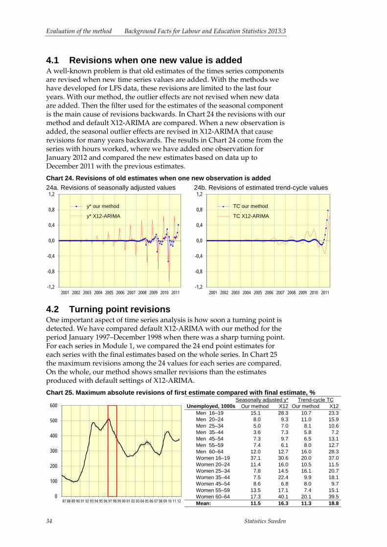
Evaluation of the method Background Facts for Labour and Education Statistics 2013:3


4.1 Revisions when one new value is added A well-known problem is that old estimates of the times series components are revised when new time series values are added. With the methods we have developed for LFS data, these revisions are limited to the last four years. With our method, the outlier effects are not revised when new data are added. Then the filter used for the estimates of the seasonal component is the main cause of revisions backwards. In Chart 24 the revisions with our method and default X12-ARIMA are compared. When a new observation is added, the seasonal outlier effects are revised in X12-ARIMA that cause revisions for many years backwards. The results in Chart 24 come from the series with hours worked, where we have added one observation for January 2012 and compared the new estimates based on data up to December 2011 with the previous estimates.

Chart 24. Revisions of old estimates when one new observation is added 24a. Revisions of seasonally adjusted values

24b. Revisions of estimated trend-cycle values

4.2 Turning point revisions One important aspect of time series analysis is how soon a turning point is detected. We have compared default X12-ARIMA with our method for the period January 1997–December 1998 when there was a sharp turning point. For each series in Module 1, we compared the 24 end point estimates for each series with the final estimates based on the whole series. In Chart 25 the maximum revisions among the 24 values for each series are compared. On the whole, our method shows smaller revisions than the estimates produced with default settings of X12-ARIMA.

Chart 25. Maximum absolute revisions of first estimate compared with final estimate, %

Seasonally adjusted y* Trend-cycle TC Unemployed, 1000s Our method X12 Our method X12

Men 16–19 15.1 28.3 10.7 23.3 Men 20–24 8.0 9.3 11.0 15.9 Men 25–34 5.0 7.0 8.1 10.6 Men 35–44 3.6 7.3 5.8 7.2 Men 45–54 7.3 9.7 6.5 13.1 Men 55–59 7.4 6.1 8.0 12.7 Men 60–64 12.0 12.7 16.0 28.3 Women 16–19 37.1 30.6 20.0 37.0 Women 20–24 11.4 16.0 10.5 11.5 Women 25–34 7.8 14.5 16.1 20.7 Women 35–44 7.5 22.4 9.9 18.1 Women 45–54 8.6 6.8 8.0 9.7 Women 55–59 13.5 17.1 7.4 15.1 Women 60–64 17.3 40.1 20.1 39.5 Mean: 11.5 16.3 11.3 18.8

-1,2

-0,8

-0,4

0,0

0,4

0,8

1,2

2001 2002 2003 2004 2005 2006 2007 2008 2009 2010 2011

rev y* w12_1

rev y* x12

-1,2

-0,8

-0,4

0,0

0,4

0,8

1,2

2001 2002 2003 2004 2005 2006 2007 2008 2009 2010 2011

rev tc w12_1

rev tc x12

0

100

200

300

400

500

600

87 88 89 90 91 92 93 94 95 96 97 98 99 00 01 02 03 04 05 06 07 08 09 10 11 12

y* our method

y* X12-ARIMA

TC our method

TC X12-ARIMA

Background Facts for Labour and Education Statistics 2013:3 The method of presentation


5 The method of presentation Cross section statistics are quantitative – here we estimate parameters. In contrast, time series statistics are much more qualitative – here we estimate patterns. “Has unemployment started to go up?” is an example of a qualitative issue that is typical for time series statistics.

The conclusion is that when we publish time series statistics, charts are essential. There are important quality issues related to charts – are the charts misleading, or interesting and informative? When we work with seasonal adjustment, it is not sufficient to discuss the methods used to estimate the time series components. We must also discuss the methods used for graphical presentation. In the system we have developed, charts are important and we describe these charts in this section.

5.1 Needle charts In Section 2.2, charts 6a and 6b are examples of two different ways of illustrating seasonally adjusted data and estimated trend-cycles. Chart 6a is the traditional way with zigzag lines for the seasonally adjusted values and a curve for the trend-curve. In Wallgren et al. (1996), we introduced the needle chart for this kind of time series data and Chart 6b is an example of this kind of chart (and also Chart 26 below). The following time series are illustrated with a needle chart: – The trend-cycle is described with the smooth curve. – Seasonally adjusted values are described by the endpoints of the needles. – The times series residuals are described by the length of each needle.

Presenting seasonally adjusted values with zigzag lines emphasizes the time series noise or the irregular pattern, and the chart gives a restless impression. The curve in the needle chart emphasizes the long-term development, but what is special to each individual point in time is also described by the needles. This is why we recommend needle charts.

5.2 Measuring and illustrating change Rate of change can be measured by comparing seasonally adjusted values, original values or estimated trend-cycle values. We compare these measures for the series describing hours worked from the Swedish LFS.

Chart 26. Hours worked, employed 15–74 years, million hours per week

125

130

135

140

145

2001 2002 2003 2004 2005 2006 2007 2008 2009 2010 2011 2012

The method of presentation Background Facts for Labour and Education Statistics 2013:3


Chart 27. Rate of change measured by seasonally adjusted values yt*/yt-1* Per cent per year

Why is seasonal adjustment important? Because then we can compare all points of time, e.g. the two last months. It is quite common to report change as per cent per month or per year comparing this month’s seasonally adjusted value with the seasonally adjusted value for the previous month. In Chart 27 we measure change as per cent per year, but if we had taken per cent per month, the chart pattern would have been the same.

Is there any meaningful information in Chart 27? Can anyone use that information for decision making? If the chart says +10% this month and -9% next month, must you then change all decisions every second month? What is the quality of the information in Chart 27?

Almost all charts based on monthly seasonally adjusted values in Sweden look like Chart 27 above and that is why we warn everyone about measuring change in this way. In Section 2.2 we stated that Swedish monthly data are too volatile, instead of seasonally adjusted values we must use trend-cycle values. In Chart 29 below, the rate of change is measured by comparing the last two values of the estimated trend-cycle (red curve, curve without dots) and that measure is much more meaningful.

Chart 28. Rate of change measured by original values yt/yt-12 Per cent per year

Another common way of measuring change is to compare this month’s original value with the value for the same month in the previous year. It is much easier to see a clear pattern in Chart 28 than in Chart 27. In Chart 28 we can see that there is an economic crisis during 2009, and it seems that the turning point in the rate of change is in the middle of 2009. But change measured in this way does not tell us what is happening now; it tells us what has happened during the last 12 months. We do not know if that

-40

-20

0

20

40

60

2001 2002 2003 2004 2005 2006 2007 2008 2009 2010 2011 2012

-10 -8 -6 -4 -2 0 2 4 6 8

10

2001 2002 2003 2004 2005 2006 2007 2008 2009 2010 2011 2012



change happened last month or 11 months ago. On the average, signals are delayed about six months by this way of measuring change. This delay can be seen in Chart 29 where this way of measuring change is compared with a measure where this month’s trend-cycle value is compared with the trend-cycle value for the previous month.

Chart 29. Rate of change measured by original values yt/yt-12 and trend TCt/TCt-1 Per cent per year

We have decided not to use the measures of change in charts 27 and 28 in the system for time series analysis of Swedish LFS data. The only measure of change we use is based on the estimated trend-cycle values.

5.3 Monthly reports Every month, a number of Excel files with tables and charts are updated. For all series presented in charts, tables with the following content are included in the same Excel file:

Original value millions of hours

worked

Corrected for calendar and moving month

Seasonally adjusted values

Estimated trend-cycle

Rate of change % per year

2012 1 141.6 139.7 142.9 143.47 -1.1 2012 2 153.0 153.2 143.0 143.36 -1.4 2012 3 154.9 153.4 143.9 143.25 -1.4 2012 4 142.6 144.5 142.4 143.14 -1.2 2012 5 145.0 148.1 142.6 143.07 -0.9 2012 6 148.0 148.4 143.5 143.03 -0.4 2012 7 93.2 92.0 142.5 143.05 0.2 2012 8 125.1 125.0 143.3 143.11 0.7

There are two different ways of presenting LFS data in charts. In Chart 30 all labour status categories for the same subpopulation are presented. Both data on persons and per cent of population are presented together. All in all, six charts are combined in the presentation for one subpopulation.

In Chart 31 we illustrate the relation between sex and age with one specific LFS category, e.g. unemployment. Chart 31 is an example of a Trellis Chart according to William Cleveland‘s terminology – a chart that consists of a table with charts in the tables cells. With this kind of chart, we can see the effects of sex and age on the category or variable that is described – in this case unemployment. It is important to have a common reference curve in all the charts that constitute Chart 31.

The presentations in charts 30 and 31 are quite different and the best idea is to include both in a presentation of LFS data.

-10 -8 -6 -4 -2 0 2 4 6 8

10

2001 2002 2003 2004 2005 2006 2007 2008 2009 2010 2011 2012

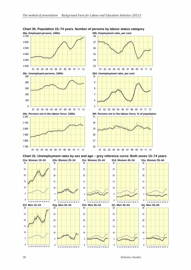
The method of presentation Background Facts for Labour and Education Statistics 2013:3


Chart 30. Population 15–74 years. Number of persons by labour status category 30a. Employed persons, 1000s

30b. Employment ratio, per cent

30c. Unemployed persons, 1000s

30d. Unemployment ratio, per cent

30e. Persons not in the labour force, 1000s

30f. Persons not in the labour force, % of population

Chart 31. Unemployment rates by sex and age – grey reference curve: Both sexes 15–74 years 31a. Women 15–24

31b. Women 25–34

31c. Women 35–44

31d. Women 45–54

31e. Women 55–64

31f. Men 15–24

31g. Men 25–34

31h. Men 35–44

31i. Men 45–54

31j. Men 55–64

4 200

4 300

4 400

4 500

4 600

4 700

01 02 03 04 05 06 07 08 09 10 11 12 63

64

65

66

67

68

01 02 03 04 05 06 07 08 09 10 11 12

0

100

200

300

400

500

01 02 03 04 05 06 07 08 09 10 11 12 5

6

7

8

9

10

01 02 03 04 05 06 07 08 09 10 11 12

1 700

1 800

1 900

2 000

2 100

2 200

01 02 03 04 05 06 07 08 09 10 11 12 26

27

28

29

30

31

01 02 03 04 05 06 07 08 09 10 11 12

0

5

10

15

20

25

30

01 02 03 04 05 06 07 08 09 10 0

5

10

15

20

25

30

01 02 03 04 05 06 07 08 09 10 0

5

10

15

20

25

30

01 02 03 04 05 06 07 08 09 10 0

5

10

15

20

25

30

01 02 03 04 05 06 07 08 09 10 0

5

10

15

20

25

30

01 02 03 04 05 06 07 08 09 10

0

5

10

15

20

25

30

01 02 03 04 05 06 07 08 09 10 0

5

10

15

20

25

30

01 02 03 04 05 06 07 08 09 10 0

5

10

15

20

25

30

01 02 03 04 05 06 07 08 09 10 0

5

10

15

20

25

30

01 02 03 04 05 06 07 08 09 10 0

5

10

15

20

25

30

01 02 03 04 05 06 07 08 09 10



5.4 Spurious correlations and disturbing factors There is always a risk that tables are published that show patterns that are disturbed by a factor that the table has not taken into account. If we publish y by x1 and x2 in a two-way table, the correlations indicated by the table can be spurious, i.e. generated by a third explanatory variable x3.

If we e.g. publish a table with unemployment rates by sex and age, the most important explanation of unemployment can be level of education. That factor can be correlated with age and this will give a spurious correlation between age and unemployment in our two-way table. The solution is to control for education by creating a three-way table. We can also compare age groups by standardising for education so that standardised unemployment rates are computed, where each age group gets the same distribution of the different levels of education.

The same problem can also disturb time series data. The population for the LFS is persons 15–74 years. However, the age distribution can change as a result of baby-boom effects. This is the case in Chart 32. During the period 2001–2012, persons born during the 1940s entered the oldest age group in the LFS and that disturbed the series regarding employment rates and labour force rates.

Chart 32a shows employment rates where the changing age distribution is not controlled. In Chart 32b the employment rates for each age group have been combined with the same standardised weights used each month. In this way the changing age distribution will not disturb. Instead of a negative long-term trend as in Chart 32a, we see a positive long-term trend. The same holds for the labour force rates in charts 32c and 32d. Chart 32c shows a negative long-term trend, but that is a spurious correlation. The negative trend is due to the changing age distribution. When we standardise for age, the long-term trend becomes positive in Chart 32d.

Chart 32. Negative long-term trends become positive when rates are age standardised 32a. Employment rates, population 15–74 years

32b. Employment rates 15–75 years, age standardised

32c. Labour force rates, population 15–74 years

32d. Labour force rates 15–75 years, age standardised

63

64

65

66

67

68

01 02 03 04 05 06 07 08 09 10 11 12

60

61

62

63

64

65

01 02 03 04 05 06 07 08 09 10 11 12

68

69

70

71

72

73

01 02 03 04 05 06 07 08 09 10 11 12 65

66

67

68

69

70

01 02 03 04 05 06 07 08 09 10 11 12

Background Facts for Labour and Education Statistics 2013:3 References


References Elezovic S., Odencrants M. and Xie Y. (2009): Summakonsistent säsongrensning 1 and 2. Project reports (in Swedish), Statistics Sweden. Eurostat (2009): ESS Guidelines on Seasonal Adjustment. Statistics Canada (2009): Quality Guidelines. Fifth Edition – October 2009. Statistics Sweden (2012): Actual Hours Worked in the Swedish LFS Background Facts – Labour and Education Statistics 2012:1. Stuckey A., Zhang and X. and McLaren C. (2004): Aggregation of Seasonally Adjusted Estimates by a Post-Adjustment. Australian Bureau of Statistics, 2004. Wallgren A., Wallgren B., Persson R., Jorner U., Haaland J. (1996): Graphing Statistics & Data – Creating Better Charts. SAGE Publications, Inc. Wallgren A., Wallgren B. (2007): Register-based Statistics – Administrative Data for Statistical Purposes. John Wiley & Sons Ltd, Chichester, England. Wallgren A., Wallgren B. (2012): Linking a system of time series – Recalculation of Labour Force Surveys 1987–1992. Methodology reports from Statistics Sweden 2012:2. Wallgren A., Wallgren B. (2013): Revising Surveys – Linking Old and New Data. Background Facts – Labour and Education Statistics 2013:2.

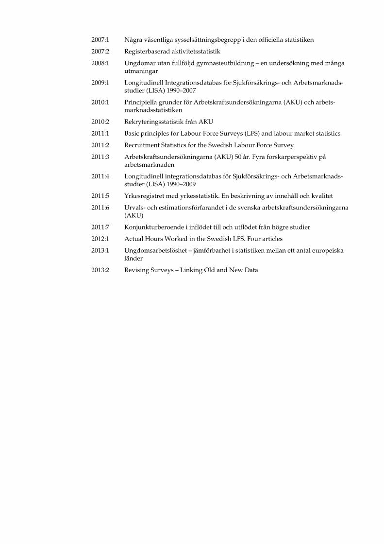
2007:1 Några väsentliga sysselsättningsbegrepp i den officiella statistiken

2007:2 Registerbaserad aktivitetsstatistik

2008:1 Ungdomar utan fullföljd gymnasieutbildning – en undersökning med många utmaningar

2009:1 Longitudinell Integrationsdatabas för Sjukförsäkrings- och Arbetsmarknads- studier (LISA) 1990–2007

2010:1 Principiella grunder för Arbetskraftsundersökningarna (AKU) och arbets- marknadsstatistiken

2010:2 Rekryteringsstatistik från AKU

2011:1 Basic principles for Labour Force Surveys (LFS) and labour market statistics

2011:2 Recruitment Statistics for the Swedish Labour Force Survey

2011:3 Arbetskraftsundersökningarna (AKU) 50 år. Fyra forskarperspektiv på arbetsmarknaden

2011:4 Longitudinell integrationsdatabas för Sjukförsäkrings- och Arbetsmarknads- studier (LISA) 1990–2009

2011:5 Yrkesregistret med yrkesstatistik. En beskrivning av innehåll och kvalitet

2011:6 Urvals- och estimationsförfarandet i de svenska arbetskraftsundersökningarna (AKU)

2011:7 Konjunkturberoende i inflödet till och utflödet från högre studier

2012:1 Actual Hours Worked in the Swedish LFS. Four articles

2013:1 Ungdomsarbetslöshet – jämförbarhet i statistiken mellan ett antal europeiska länder

2013:2 Revising Surveys – Linking Old and New Data

www.scb.se Arbetsmarknads- och utbildningsstatistik

Bakgrundsfakta

2005:2

Svenska hälsoräkenskaper+ enrad

+ännu en radoch den 4:e

ISSN 1654-465X (Online)

All officiell statistik finns på: www.scb.se Statistikservice: tfn 08-506 948 01

All official statistics can be found at: www.scb.se Statistics service: phone +46 8 506 948 01

background facts: consistent seasonal adjustment · 2018-08-21 · anders wallgren and britt...

Documents