avance 1d and 2d course - north central...
TRANSCRIPT

Avance 1D/2D BRUKER 1
Avance 1D and 2D Course
© February 20, 2001, Bruker AGFällanden, Switzerland
Version 010220

2 BRUKER Avance 1D/2D

Avance 1D/2D BRUKER 3
1 INTRODUCTION ....................................................................................................................................... 9
1.1 AN IMPORTANT NOTE ON POWER LEVELS ................................................................................................ 91.2 NMR SPECTROMETER........................................................................................................................... 101.3 CLASSICAL DESCRIPTION OF NMR ........................................................................................................ 101.4 SPIN OPERATORS OF A ONE-SPIN SYSTEM.............................................................................................. 11
1.4.1 Effect of rf-Pulses .................................................................................................................... 121.4.2 Effect of Chemical Shift Evolution............................................................................................ 121.4.3 Effect of Scalar Coupling ......................................................................................................... 13
1.5 SENSITIVITY OF NMR EXPERIMENTS ..................................................................................................... 141.6 USEFUL COUPLING CONSTANTS............................................................................................................. 14
1.6.1 Coupling Constants: nJCH ......................................................................................................... 141.6.2 Coupling Constants of Hydrocarbons: nJHH .............................................................................. 15
2 PREPARING FOR ACQUISITION ......................................................................................................... 17
2.1 SAMPLE PREPARATION .......................................................................................................................... 172.2 BRUKER NMR SOFTWARE ..................................................................................................................... 17
2.2.1 Predefined Parameter Sets....................................................................................................... 182.2.2 XWinNMR parameters and commands ..................................................................................... 202.2.3 Changes for XWinNMR 3.0 ...................................................................................................... 24
2.3 TUNING AND MATCHING THE PROBE...................................................................................................... 242.4 TUNING AND MATCHING 1H (NON ATM PROBES) .................................................................................. 25
2.4.1 Set the Parameters................................................................................................................... 252.4.2 Start Wobbling......................................................................................................................... 262.4.3 Tune and Match....................................................................................................................... 26
2.5 TUNING AND MATCHING 13C (NON ATM PROBES) ................................................................................. 272.5.1 Set the Parameters................................................................................................................... 272.5.2 Start Wobbling, Tune and Match.............................................................................................. 27
2.6 LOCKING AND SHIMMING ...................................................................................................................... 282.6.1 Locking ................................................................................................................................... 282.6.2 Shimming ................................................................................................................................ 292.6.3 Optimize lock settings (optional) .............................................................................................. 29
3 BASIC 1H ACQUISITION AND PROCESSING ..................................................................................... 31
3.1 INTRODUCTION ..................................................................................................................................... 313.1.1 Sample .................................................................................................................................... 313.1.2 Preparation ............................................................................................................................. 31
3.2 SPECTROMETER AND ACQUISITION PARAMETERS ................................................................................... 323.3 CREATE A NEW FILE DIRECTORY FOR THE DATA SET ............................................................................. 323.4 SET UP THE SPECTROMETER PARAMETERS............................................................................................. 323.5 SET UP THE ACQUISITION PARAMETERS................................................................................................. 333.6 ACQUISITION ........................................................................................................................................ 343.7 PROCESSING ......................................................................................................................................... 343.8 PHASE CORRECTION.............................................................................................................................. 353.9 WINDOWING ......................................................................................................................................... 353.10 INTEGRATION...................................................................................................................................... 37
4 PULSE CALIBRATION: PROTONS....................................................................................................... 39
4.1 INTRODUCTION ..................................................................................................................................... 394.2 PROTON OBSERVE 90° PULSE ................................................................................................................ 39
4.2.1 Preparation ............................................................................................................................. 394.2.2 Optimize the Carrier Frequency and the Spectral Width ........................................................... 404.2.3 Define the Phase Correction and the Plot Region ..................................................................... 414.2.4 Calibration: High Power ......................................................................................................... 414.2.5 Calibration: Low Power for MLEV Pulse Train (TOCSY)......................................................... 424.2.6 Calibration: Low Power for ROESY Spinlock........................................................................... 43
5 BASIC 13C ACQUISITION AND PROCESSING .................................................................................... 45
5.1 INTRODUCTION ..................................................................................................................................... 45

4 BRUKER Avance 1D/2D
5.1.1 Sample .................................................................................................................................... 455.1.2 Prepare a New Data Set........................................................................................................... 45
5.2 ONE-PULSE EXPERIMENT WITHOUT 1H DECOUPLING ............................................................................... 455.3 ONE-PULSE EXPERIMENT WITH 1H DECOUPLING .................................................................................... 48
6 PULSE CALIBRATION: CARBON......................................................................................................... 51
6.1 CARBON OBSERVE 90° PULSE ............................................................................................................... 516.1.1 Preparation ............................................................................................................................. 516.1.2 Optimize the Carrier Frequency and the Spectral Width ........................................................... 526.1.3 Define the Phase Correction and the Plot Region ..................................................................... 526.1.4 Calibration: High Power ......................................................................................................... 52
6.2 PROTON DECOUPLING 90° PULSE DURING 13C ACQUISITION................................................................... 546.2.1 Sample .................................................................................................................................... 546.2.2 Pulse Sequence ........................................................................................................................ 546.2.3 Set the 1H Carrier Frequency................................................................................................... 546.2.4 Set the 13C Carrier Frequency and the Spectral Width .............................................................. 556.2.5 Calibration: High Power ......................................................................................................... 576.2.6 Calibration: Low Power for WALTZ-16 Decoupling................................................................. 58
6.3 CARBON DECOUPLER 90° PULSE (INVERSE MODE)................................................................................. 586.3.1 Sample .................................................................................................................................... 586.3.2 Preparation ............................................................................................................................. 596.3.3 Set the 13C Carrier Frequency.................................................................................................. 596.3.4 Set the 1H Carrier Frequency and the Spectral Width ............................................................... 616.3.5 Preparations for the Inverse Pulse Calibration......................................................................... 626.3.6 Calibration: High Power ......................................................................................................... 646.3.7 Calibration: Low Power for GARP Decoupling........................................................................ 64
6.4 1D INVERSE TEST SEQUENCE ................................................................................................................ 65
7 ADVANCED 1D 13C EXPERIMENTS ..................................................................................................... 69
7.1 CARBON EXPERIMENTS WITH GATED 1H-DECOUPLING ........................................................................... 697.1.1 Plotting 1D 13C Spectra ........................................................................................................... 71
7.2 DEPT................................................................................................................................................... 727.2.1 Acquisition and Processing ...................................................................................................... 737.2.2 Reference Spectra .................................................................................................................... 737.2.3 Create a New Data Set............................................................................................................. 737.2.4 Spectrum Acquisition ............................................................................................................... 747.2.5 Processing of the Spectrum ...................................................................................................... 757.2.6 Other spectra........................................................................................................................... 757.2.7 Plot the spectra........................................................................................................................ 75
7.3 APT (ATTACHED PROTON TEST) ........................................................................................................... 777.3.1 Acquisition and Processing ...................................................................................................... 777.3.2 Reference Spectra .................................................................................................................... 777.3.3 Create a New Data Set............................................................................................................. 787.3.4 Spectrum Acquisition ............................................................................................................... 787.3.5 Processing of the Spectrum ...................................................................................................... 797.3.6 Plot the spectra........................................................................................................................ 79
8 COSY......................................................................................................................................................... 81
8.1 INTRODUCTION ..................................................................................................................................... 818.2 MAGNITUDE COSY .............................................................................................................................. 81
8.2.1 Pulse Sequence ........................................................................................................................ 828.2.2 Acquisition of the 2D COSY Spectrum...................................................................................... 828.2.3 Processing of the 2D COSY Spectrum ...................................................................................... 838.2.4 Plotting the Spectrum............................................................................................................... 85
8.3 DOUBLE-QUANTUM FILTERED (DQF) COSY......................................................................................... 868.3.1 Pulse Sequence........................................................................................................................ 868.3.2 Acquisition and Processing ...................................................................................................... 868.3.3 Phase correct the spectrum ...................................................................................................... 888.3.4 Plot the spectrum..................................................................................................................... 88
8.4 DOUBLE-QUANTUM FILTERED COSY USING PULSED FIELD GRADIENTS (GRASP-DQF-COSY) ............. 898.4.1 Pulse Sequence ........................................................................................................................ 90

Avance 1D/2D BRUKER 5
8.4.2 Acquisition and Processing ...................................................................................................... 90
9 TOCSY ...................................................................................................................................................... 93
9.1 INTRODUCTION ..................................................................................................................................... 939.2 ACQUISITION ........................................................................................................................................ 949.3 PROCESSING ......................................................................................................................................... 959.4 PHASE CORRECTION.............................................................................................................................. 969.5 PLOT THE SPECTRUM............................................................................................................................. 97
10 ROESY..................................................................................................................................................... 99
10.1 INTRODUCTION ................................................................................................................................... 9910.2 ACQUISITION .....................................................................................................................................10010.3 PROCESSING ......................................................................................................................................10110.4 PHASE CORRECTION AND PLOTTING ...................................................................................................102
11 NOESY....................................................................................................................................................103
11.1 INTRODUCTION ..................................................................................................................................10311.2 ACQUISITION AND PROCESSING ..........................................................................................................104
11.2.1 Optimize Mixing Time.............................................................................................................10511.2.2 Acquire the 2D data set...........................................................................................................106
11.3 PROCESSING ......................................................................................................................................10611.4 PHASE CORRECTION AND PLOTTING ...................................................................................................107
12 XHCORR................................................................................................................................................109
12.1 INTRODUCTION ..................................................................................................................................10912.2 ACQUISITION .....................................................................................................................................110
12.2.1 Proton Reference Spectrum.....................................................................................................11012.2.2 Carbon Reference Spectrum....................................................................................................11012.2.3 Acquire the 2D Data Set .........................................................................................................111
12.3 PROCESSING ......................................................................................................................................11212.4 PLOTTING THE SPECTRUM ..................................................................................................................113
13 COLOC...................................................................................................................................................115
13.1 INTRODUCTION ..................................................................................................................................11513.2 ACQUISITION AND PROCESSING ..........................................................................................................116
14 HMQC ....................................................................................................................................................119
14.1 INTRODUCTION ..................................................................................................................................11914.2 ACQUISITION .....................................................................................................................................120
14.2.1 Optimize d7 (only for HMQC with BIRD)................................................................................12214.2.2 Acquire the 2D data set...........................................................................................................122
14.3 PROCESSING ......................................................................................................................................12214.4 PHASE CORRECTION...........................................................................................................................12314.5 PLOTTING ..........................................................................................................................................123
15 HMBC.....................................................................................................................................................125
15.1 INTRODUCTION ..................................................................................................................................12515.2 ACQUISITION AND PROCESSING ..........................................................................................................126
16 PROTON-CARBON INVERSE SHIFT CORRELATION- EXPERIMENTS USING PULSED FIELDGRADIENTS...............................................................................................................................................129
16.1 INTRODUCTION ..................................................................................................................................12916.2 GRASP-HMQC.................................................................................................................................12916.3 GRASP-HMBC.................................................................................................................................13016.4 GRASP-HSQC..................................................................................................................................13116.5 ACQUISITION AND PROCESSING ..........................................................................................................132
17 1D NOE DIFFERENCE .........................................................................................................................137
17.1 INTRODUCTION ..................................................................................................................................13717.2 ACQUISITION .....................................................................................................................................138
17.2.1 Create a new file directory......................................................................................................138

6 BRUKER Avance 1D/2D
17.2.2 Proton reference spectrum ......................................................................................................13817.2.3 Select the resonances for irradiation .......................................................................................13917.2.4 Set up the acquisition parameters............................................................................................14017.2.5 Optimize the irradiation power and duration...........................................................................14017.2.6 Perform the multiple NOE experiment.....................................................................................141
17.3 PROCESSING ......................................................................................................................................14217.3.1 Perform the Phase Correction.................................................................................................14217.3.2 Create NOE Difference Spectra ..............................................................................................14217.3.3 Quantitate the NOE ................................................................................................................143
18 HOMONUCLEAR DECOUPLING.......................................................................................................145
18.1 INTRODUCTION ..................................................................................................................................14518.2 ACQUISITION .....................................................................................................................................146
18.2.1 Create a new file directory......................................................................................................14618.2.2 Proton reference sepctrum ......................................................................................................14618.2.3 Selection of irradiation frequency ...........................................................................................14618.2.4 Setting up the homo decoupling parameters.............................................................................147
19 T1 MEASUREMENT..............................................................................................................................149
19.1 INTRODUCTION ..................................................................................................................................14919.2 ACQUISITION .....................................................................................................................................150
19.2.1 Write the variable delay list ....................................................................................................15019.2.2 Set up the acquisition parameters............................................................................................15119.2.3 Acquire the 2D data set...........................................................................................................151
19.3 PROCESSING ......................................................................................................................................15219.3.1 Write the integral range file and baseline point file .................................................................152
19.4 T1 CALCULATION ...............................................................................................................................15319.4.1 Check T1 curves ......................................................................................................................15419.4.2 Check numerical results..........................................................................................................15419.4.3 T1 parameters .........................................................................................................................155
19.5 CREATE A STACKED PLOT ..................................................................................................................155
20 SELECTIVE EXCITATION..................................................................................................................159
20.1 INTRODUCTION ..................................................................................................................................15920.2 SELECTIVE PULSE CALIBRATION.........................................................................................................159
20.2.1 Proton reference spectrum ......................................................................................................16020.2.2 Selective one-pulse sequence...................................................................................................16020.2.3 Define the pulse shape ............................................................................................................16020.2.4 Acquire and process the selective one-pulse spectrum .............................................................16020.2.5 Perform the pulse calibration..................................................................................................162
20.3 SELECTIVE COSY..............................................................................................................................16320.3.1 Acquisition .............................................................................................................................16420.3.2 Processing..............................................................................................................................165
20.4 SELECTIVE TOCSY............................................................................................................................16620.4.1 Variable Delay List.................................................................................................................16720.4.2 Acquisition .............................................................................................................................16720.4.3 Processing..............................................................................................................................169
21 APPENDIX A: ARTIFACTS IN 2D-NMR EXPERIMENTS................................................................171
21.1 INTRODUCTION ..................................................................................................................................17121.1.1 Why do artifacts occure? ........................................................................................................171
21.2 THE DOUBLE-QUANTUM FILTERED COSY EXPERIMENT .....................................................................17221.2.1 Rapid Scanning Artifacts.........................................................................................................17221.2.2 Overload of the receiver..........................................................................................................17421.2.3 The ‘diamond pattern’............................................................................................................175
21.3 THE HOMONUCLEAR J-RESOLVED EXPERIMENT ..................................................................................17621.3.1 The Effect of digital resolution and tilting of the spectrum .......................................................176
21.4 INVERSE EXPERIMENTS ......................................................................................................................17721.4.1 Incorrect proton pulses ...........................................................................................................177Rapid scanning artifacts .......................................................................................................................178
21.5 THE TOCSY EXPERIMENT..................................................................................................................179

Avance 1D/2D BRUKER 7
21.5.1 Sample heating due to the spin lock sequence ..........................................................................17921.5.2 Solvent suppression and trim pulses ........................................................................................180
22 APPENDIX B: THEORETICAL BACKGROUND OF NMR ..............................................................183
22.1 INTRODUCTION ..................................................................................................................................18322.2 CLASSICAL DESCRIPTION OF NMR .....................................................................................................18322.3 SPIN OPERATORS OF A ONE-SPIN SYSTEM ...........................................................................................18522.4 THE THERMAL EQUILIBRIUM STATE ...................................................................................................18522.5 EFFECT OF RF-PULSES .......................................................................................................................18622.6 THE HAMILTONIAN: EVOLUTION OF SPIN SYSTEMS IN TIME ................................................................187
22.6.1 Effect of Chemical Shift Evolution...........................................................................................18822.7 OBSERVABLE SIGNALS AND OBSERVABLE OPERATORS........................................................................18922.8 OBSERVING TWO AND MORE SPIN SYSTEMS .......................................................................................191
22.8.1 Effect of Scalar Coupling ........................................................................................................19222.8.2 Evolution under Weak Coupling..............................................................................................19322.8.3 The Signal Function of a Coupled Spectrum............................................................................194
22.9 SIMPLIFICATION SCHEMES ON A THREE-SPIN SYSTEM.........................................................................19522.10 THE COSY EXPERIMENT..................................................................................................................19622.11 SUMMARY AND USEFUL FORMULAE..................................................................................................201
22.11.1 Effects on Spins in the Product Operator Formalism...........................................................20122.11.2 Mathematical Relations......................................................................................................202

8 BRUKER Avance 1D/2D

Avance 1D/2D BRUKER 9
1 IntroductionThis manual gives an introduction into basic one- and two-dimensionalnuclear magnetic resonance (NMR) spectroscopy. After a short introductionthe acquisition of basic 1D 1H and 13C NMR spectra is described in theChapters 3 to 7. Homonuclear 2D [1H,1H] correlation spectra are described inChapter 8 (COSY), 9 (TOCSY), 10 (ROESY) and 11 (NOESY).Heteronuclear 2D [13C,1H] correlation experiments are described in Chapter12 (XHCORR), 13 (COLOC), 14 (HMQC) and 15 (HMBC). The Chapter 16contains the description of inverse 2D [13C,1H] correlation experiments usingpulsed field gradients, and some special NMR experiments are described inChapters 0 to 20.
1.1 An Important Note on Power Levels
Several places throughout this manual, the user is asked to set the powerlevels pl1, pl3, etc. to the “high power” level for the corresponding channel(f1 or f2). In order to avoid damaging the probehead or other hardwarecomponents, the user is advised to use only the power levels indicated inTable 1 below, if no other information (e.g. final acceptance tests) isavailable.
Note that these “power levels” are really attenuation levels, and so a highervalue corresponds to a lower power. Also note that these power levelspertain only to the specific spectrometers and amplifiers listed below, whichcorrespond to the AVANCE instruments as of July 2000. It is assumed thatno correction tables (CORTAB) are existing.
Table 1: Suggested “Proton and Carbon High Power” Levels for AvanceInstruments
Nucleus Spectrometer Amplifier Power Level
Avance BLA2BB ≥ + 3dB
BLARH100 ≥ + 3dB
BLAXH300/50 ≥ 0dB
Avance DPX BLAXH20 = - 6dB
BLAXH40 = - 3dB
BLAXH100/50 ≥ 0dB
Avance DRX BLAXH150/50 ≥ 0dB
BLAXH300/50 ≥ 0dB
1H
Avance DMX BLARH100 ≥ + 3dB

10 BRUKER Avance 1D/2D
Nucleus Spectrometer Amplifier Power Level
Avance BLA2BB ≥ + 6dB
BLAX300/50 ≥ + 6dB
BLAX300 ≥ + 6dB
BLAX500 ≥ + 9dB
Avance DPX BLAXH20 = - 6dB13C BLAXH40 = - 6dB
BLAXH100/50 ≥ - 3dB
Avance DRX BLAXH40 ≥ - 3dB
BLAXH150/50 ≥ 0dB
BLAXH300/50 ≥ 6dB
Avance DMX BLAX300 ≥ + 6dB
BLAX500 ≥ + 9dB
1.2 NMR Spectrometer
The NMR spectrometer consists of three major components: (1) Thesuperconducting magnet with the probe, which contains the sample to bemeasured; (2) The console, which contains all the electronics used fortransmission and reception of radio frequency (rf) pulses through the pre-amplifier to the probe; (3) The computer, from where the operator runs theexperiments and processes the acquired NMR data.
1.3 Classical Description of NMR
A more complete theoretical description of NMR is given in chapter 21.
Among the various atomic nuclei, about a hundred isotopes possess anintrinsic angular momentum, called spin and written Ih . They also possess amagnetic moment µ which is proportional to their angular momentum:
Ihγµ =
where γ is the gyromagnetic ratio.
The Larmor theorem states that the motion of a magnetic moment in amagnetic field B0 is a precession around that field, where the precessionfrequency is given by:
00 Bγω −= Larmor frequency

Avance 1D/2D BRUKER 11
By convention, the external static field (B0) is assumed to be along the z-axisand the transmitter/receiver coil along either the x- or y-axis. After the samplehas been inserted into the magnetic field it shows a magnetization vectorMr
along the z-axis. In this state, no NMR signal is observed, as we have notranverse rotating magnetization.
By applying an additional rotating magnetic field B1 in the x-y-plane, theorientation of M
rcan be tilted into the x-y plane where it precesses around
the total magnetic field, e.g. the vector sum of B0 and B1. Such a rotatingmagnetic field is obtained by applying rf-pulses, and the components ofMr
are described by the Bloch equations:
1
1
0
BMMdtd
MBMdtd
Mdtd
ryz
zry
rx
γ
γ
−=
=
=
Assuming the magnetization at time 0 to be along the z-axis with amplitudeM0, we find the following solution to the above equation:
)cos()(
)sin()(
10
10
tBMtM
tBMtM
z
ry
γγ
==
The magnetization vector is precessing around the B1 axis which is alignedwith the x-axis of the reference system. If we choose the time t of suitableduration, we obtain:
21πγβ == tB
which is defined as the 90 degree pulse creating maximum y-magnetization,which in turn yields maximal signal intensity.
1.4 Spin Operators of a One-Spin System
All NMR experiments start from the thermal equilibrium. In thermalequilibrium, the classical description gives a magnetic moment parallel to thestatic field, Mz. In the Spin Operator formalism, this is described by:
zeq I=σ
where σeq is the equilibrium density matrix representing the state of the spinsystem under investigation.
Now there are only two basic types of evolutions: (1) An externalperturbation, e.g. a rf-pulse, or (2) an unperturbed evolution which willeventually bring the system back to the thermal equilibrium.

12 BRUKER Avance 1D/2D
1.4.1 Effect of rf-PulsesThe effect of an rf-pulse is that of a rotation along the pulse axes according tothe following calculus rules:
ββββ
ββ
ββ
β
β
β
β
β
β
sincos
sincos
sincos
sincos
zyy
zxx
yy
xx
xzz
yzz
III
III
II
II
III
III
x
y
y
x
y
x
+ →− →
→ →
+ →
− →
If the flip angle β = 90° then:
z90
y,x
y,x90
z
II
IIx,y
x,y
m →
± →
We find the expected result, that a 90° pulse will generate transversemagnetization. The rest of this chapter will be concerned with finding outabout the fate of this transverse magnetization in time.
We introduced tacitly the arrow notation, where we find on the left side thesystem before and on the right side after the specific evolution under theoperator noted above the arrow. This notation is simple, very convenient andnot only limited to the description of rf-pulses. We will discuss this notation inmore details in the next section.
1.4.2 Effect of Chemical Shift EvolutionThe so-called chemical shift Hamiltonian is given by:
H zI⋅= δ
where δ is the chemical shift of the corresponding nucleus in the NMRspectrum ( ωωδ −= 0 where ω0 is the Larmor frequency of the spin and ω thecarrier frequency of the interaction frame).
The calculus rules for the chemical shift evolution are the following:
)t sin(I)t cos(II
)t sin(I)t cos(II
II
xytI
y
yxtI
x
ztI
z
z
z
z
δ−δ →δ+δ →
→
⋅⋅δ
⋅⋅δ
⋅⋅δ
The time t is the period, during which the Hamiltonian is valid. TheHamiltonian of a spin system can change with time, for example if theexperimental setup prescribes first a rf-pulse and then a period ofunperturbed evolution. For the calculus rules it is mandatory, that eachHamiltonian is time independent during the time t.
What’s the general idea? The whole NMR experiment is divided into timeintervals, during which the Hamiltonian can be made time independent by

Avance 1D/2D BRUKER 13
choice of a suitable interaction frame. Typical experiments are divided inpulse intervals and free evolution times.
During the pulses, the chemical shift and scalar coupling interaction isignored. Only the applied B1 field is considered. This approach is justified forpulses with tpulse«T1,T2.
1.4.3 Effect of Scalar CouplingApart from the chemical shift, there is a second very import interactionbetween spins, the scalar coupling. The scalar depends on the mediation ofelectrons, which are confined in orbitals around both nuclei. The scalarcoupling is expressed in Hz and noted as J. The operator expression for thescalar coupling is:
z2z112 II J 2π
The above Hamiltonian expresses the scalar coupling between spin 1 andspin 2 with a coupling constant J12. The evolution Hamiltonian for this spinsystem is then:
H z2z112z22z11 II J 2I I π+δ+δ=
To calculate the effect of this Hamiltonian, it is divided into 3 parts:
z2z112
z22
z11
II J 2I I
πδδ
which are applied in sequence, where this sequence is arbitrary. After a 90°pulse has been applied to the two spins, we first calculate the two chemicalshift terms:
12y22x2
1y11x1tI
z21y11x1tI
z2z1eq
)t sin(I)t cos(I
)t sin(I)t cos(I
I)t sin(I)t cos(IIIz22
z11
σ⇒δ+δ+δ+δ →
+δ+δ →+=σ⋅⋅δ
⋅⋅δ
The next step will be to compute the evolution under the scalar coupling.
The scalar coupling term can be evaluated with a simple set of rules:
y2x1t II J 2
y2x1
12x112z2y1t II J 2
z2y1
12y112z2x1t II J 2
z2x1
12z2x112y1t II J 2
y1
12z2y112x1t II J 2
x1
z1t II J 2
z1
II 2II2
)tJsin(I)tJcos(II 2II2
)tJsin(I)tJcos(II 2II2
)tJsin(II 2)tJcos(II
)tJsin(II 2)tJcos(II
II
z2z112
z2z112
z2z112
z2z112
z2z112
z2z112
→⋅π−π →⋅π+π →⋅π−π →π+π →
→
π
π
π
π
π
π
which can then be applied to the various terms of σ1 above:

14 BRUKER Avance 1D/2D
2
212x2z112y2
212y2z112x2
112z2x112y1
112z2y112x1t II J 2
1
)tsin()tJsin(II 2)tJcos(I
)tcos()tJsin(II 2)tJcos(I
)tsin()tJsin(II 2)tJcos(I
)tcos()tJsin(II 2)tJcos(Iz2z112
σ=δ⋅π−π+δ⋅π+π+δ⋅π−π+δ⋅π+π →σ π
References: O. W. Sørensen, G.W. Eich, M. H. Levitt, G. Bodenhausen, R.R. Ernst, Progres in NMR Spectroscopy, 16, 163 (1983).
1.5 Sensitivity of NMR Experiments
The sensitivity of NMR experiments is given by the signal to noise ratio:
( )T
nsBTNNS detexc
2/302/
γγ=
S/N = signal to noise ratioN = number of spins in the system (sample concentration)γexc = gyromagnetic ratio of the excited nucleusγdet = gyromagnetic ratio of the detected nucleusns = number of scansB0 = external magnetic fieldT2 = transverse relaxation time (determines the line width)T = sample temperature
(Comment: here we can already see that it might be useful for a better signalto noise ratio to excite one kind of nuclei and detect another kind with a bettergyromagnetic ratio in the same experiment. This is done in inverseexperiments which are described in sections 14 to 16).
1.6 Useful Coupling Constants
Many NMR constants such as chemical shift ranges, sensitivities, commonNMR solvent properties etc. can be found in the Bruker Almanac. Here weadded the values of some common coupling constants that are used moreoften as parameters (cnst1 – cnst5) in some pulse programs.
1.6.1 Coupling Constants: nJCH
As a rule of thumb it is possible to estimate the 1JCH coupling constant fromthe following equation: 1JCH ~ 500*(fractional CH s character). That is: 125Hz< 1JCH < 250Hz, so that 1JCH = 145Hz is a good approximation in most cases.
The values of 2JCH coupling constants increase with increasing HCαCβangles and with the electronegativity of the Cβ substituent. They varybetween –5 and 50Hz.

Avance 1D/2D BRUKER 15
The 3JCH coupling constants are mostly positive and are maximal at CCCHangles of 0° and 180°. The values for trans couplings are larger as for ciscouplings (Karplus relation).
Table 2: Useful CH Coupling Constants
Compound 1JCH in HzEthane 124.9Acetonitrile 136.0Ethene 156Benzene 159Dichloromethane 178.0Chloroform 209.0Formaldehyde 222.0
System 2JCH in HzC(sp3)C(sp3)H -10 to +6C(sp3)C(sp2)H 0 to +30C(sp2)C(sp3)H -7 to -4C(sp2)C(sp2)H -4 to +14
System 3JCH in HzC(sp3)C(sp3)C(sp3)H 0 to 8C(sp3)C(sp2) C(sp2)H 0 to 20C(sp2)C(sp2) C(sp3)H 0 to 20
Jtrans > Jcis
References: H.-O. Kalinowski, S. Berger, S. Braun; 13C-NMR-Spektroskopie;Georg Thieme Verlag; Stuttgart, New York.
1.6.2 Coupling Constants of Hydrocarbons: nJHH
Usually 2JHH coupling constants are negative and vary in a range between-0.5Hz and -15Hz in hydrocarbons. 3JHH coupling constants are mostlypositive and usually range from 2 up to 18Hz. The n>3JHH coupling is positiveor negative with smaller absolute values, that range from 0 to 3Hz. TheKarplus relation is also valid: Jtrans > Jcis.
Table 3: Useful HH Coupling Constants
System 2JHH in HzHC(sp3)H -12 to -15HC(sp2)H -0.5 to -3
System 3JHH in HzHC(sp3)C(sp3)H 2 to 9HC(sp3)C(sp2)H 4 to 10HC(sp2)C(sp2)H 6 to 18HC(sp3)CHO 1 to 3HC(sp2)CHO 2 to 4
System 4JHH (abs. value) in HzHC(sp3)C(sp3)C(sp3)H 0HC(sp3)C(sp2)C(sp2)H 0 to 3HC(sp)C(sp)C(sp3)H 2 to 3

16 BRUKER Avance 1D/2D
Heteroatoms with considerable I or M effect can shift the J valuesdramatically.

Avance 1D/2D BRUKER 17
2 Preparing for Acqu isition
2.1 Sample Preparation
The sample quality can have a significant impact on the quality of the NMRspectrum. The following is a brief list of suggestions to ensure high samplequality:
• Always use clean and dry sample tubes to avoid contamination of thesample.
• Always use high quality sample tubes to avoid difficulties with shimming.
• Filter the sample solution.
• Always use the same sample volume or solution height (recommendedvalues: 0.6 ml or 4 cm of solution for 5 mm sample tubes, 4.0 ml or 4 cmof solution for 10 mm sample tubes). This minimizes the shimming thatneeds to be done between sample changes.
• Use the depth gauge to position the sample tube in the spinner. This isdiscussed further in Chapter 5 ‘Sample Positioning' of the BSMS User'sManual.
• Check that the sample tube is held tightly in the spinner so that it does notslip during an experiment.
• Wipe the sample tube clean before inserting it into the magnet.
• For experiments using sample spinning, be sure that the spinner,especially the reflectors, are clean. This is important for maintaining thecorrect spinning rate.
2.2 Bruker NMR software
There are three major tasks that are controlled by the NMR software:acquisition, processing and plotting. The XWinNMR program is the userinterface for all of these tasks. The commands can either be called up byselecting the menu items or by typing the appropriate command in thecommand line followed by RETURN. There are many parameters that areimportant for each job and they can be accessed and edited by the user.These parameters and the measured data as well as the processed spectraare stored in datasets which are specified by names, experiment numbers(expno) and processing numbers (procno).

18 BRUKER Avance 1D/2D
Each parameter can be accessed directly by entering it’s name in thecommand line followed by RETURN or in the eda, edp or edg window foracquisition-, processing- or plotting parameters respectively. Since thesepanels contain all possible parameters and are rather large, it is often moreconvenient to use somewhat more reduced parameter editor interfaces. Theased command opens the panel for the acquisition parameters that are ofimportance only for the selected pulse program. Here the parameters arealso commented on.
2.2.1 Predefined Parameter SetsThe XWinNMR philosophy is to work with predefined parameter sets that aresuitable for most of the NMR tasks and experiments you are facing. Theseparameter sets include the pulse program, acquisition and processing AUprograms as well as all other necessary parameters except spectrometerspecific values for pulse lengths and power levels. These standard parametersets usually have the same base name as the corresponding pulse program.Each parameter set can be called up into a dataset of your choice by thecommand rpar. You can modify the parameters and save the newparameter set by the command wpar. Bruker predefined parameter sets arewritten in capital letters, and we recommend that you do not change them butrather create new ones that you can use just as well.
Therefore the most simple way to run a certain experiment is to create a newdataset with a specific name, using the command edc. Then you would readthe corresponding parameter set by rpar (i.e. rpar PROTON all), set thepulse lengths and power levels by xau gpro (getprosol in XwinNMR 3.0)and type xaua to start the acquisition. (It is assumed that the sample isshimmed and the probe is matched and tuned for the specific nuclei). If youare using the Bruker predefined parameter sets, you can always process thedata by typing xaup.
The following list is a short summary of the most commonly usedexperiments and the corresponding parameter sets. The emphasis is on thespectroscopic information that you will get from the experiments rather thanon the type of experiment. (For the experiments in this table, it is alwaysrecommended to use the gradient version of the experiment if you have therequired z-gradient hardware. These experiments usually require less timethan the ones without gradients).

Avance 1D/2D BRUKER 19
Table 4: Short List of Typical Experiments, Parameter Sets and What They Do
Atom / Group Information (1D Experiments) a.k.a. Parameter SetH 1H chemical shift and coupling 1D1H PROTON
C 13C chemical shift, 1H decoupled (signalenhancement, integration not possible)
1D13C C13CPD
C 13C chemical shift, 1H coupled (signalenhancement, integration not possible)
1D13C C13GD
CH, CH2, CH313C chemical shift, select CH, CH2 andCH3 signals only (same phase)
DEPT45 C13DEPT45
CH 13C chemical shift, select CH signalsonly
DEPT90 C13DEPT90
CH, CH313C chemical shift, select CH and CH3signals only (opposite phase)
DEPT135 C13DEPT135
Correlation Information (2D Experiments) a.k.a. Parameter Set
H–H 1H/1H nearest neighbor, through bondchemical shift correlation
COSY COSYGPSW1
COSY45SWH–H 1H/1H nearest neighbor, through bond
chemical shift correlation plus couplingconstants
DQF-COSY
COSYGPDFPHSW1
COSYDQFPHSW
H–(–)nH1H/1H total spin system through bondchemical shift correlation
TOCSY MLEVPHSW
C–H Sensitive 1H/13C directly boundchemical shift correlation (one bond),lower resolution in 13C dimension
HSQCHMQC
INVIGPPHSW1
INV4SW
C–H Sensitive 1H/13C directly boundchemical shift correlation (one bond),lower resolution in 13C dimension (smallmolecules, solemnly select 13C/1H not12C/1H)
BIRD-HMQC
INVBSW
C–H Insensitive 1H/13C directly boundchemical shift correlation (one bond),high resolution in 13C dimension
HETCOR HCCOSW
C–(–)nH Sensitive 1H/13C long range chemicalshift correlation (more than one bond),lower resolution in 13C dimension
HMBC INV4GPLPLRNDSW1
INV4LPLRNDSWC–(–)nH Insensitive 1H/13C long range chemical
shift correlation (one and more bonds),high resolution in 13C dimension
COLOC HCCOLOCSW
H… H1H/1H non bound structural neighbor,through space chemical shift correlation(small molecules, low fields)
ROESY ROESYPHSW
H… H1H/1H non bound structural neighbor,through space chemical shift correlation(large molecules, proteins)
NOESY NOESYPHSW
In most of the 2D parameter sets there is a spectral width optimizationimplemented (PULSEPROGRAMSW). So if you acquire the corresponding1D experiments in the previous experiment number the spectral width for the2D will be optimized according to the 1D information.
1 z-gradient hardware required

20 BRUKER Avance 1D/2D
A complete list of parameter sets can be called up by typing rpar without afollowing name. The nomenclature of the parameter sets follows the rules forthe nomenclature of the pulse programs. They can be found in the file:$XWinNMRHome/exp/stan/nmr/lists/pp/Pulprog.info
However in this manual, we focus on the manual setup of the experimentsfrom scratch and the optimization of the corresponding parameters. thereforethe rpar command will not be used throughout this text.
2.2.2 XWinNMR parameters and commandsA list of commonly used acquisition and processing commands andparameter names as well as a description of the corresponding command orparameter is given in short in the tables below.
Table 5: General Commands and AU Programs
setres customize the XwinNMR interfaceedmac edit or create an XWinNMR macroedau edit or create an XWinNMR AU programedpul edit or create an XWinNMR pulse programxaulistall_au
create a file called “listall” in your home directory with a list of allavailable AU programs including short descriptions
edcpul edit the current pulse program
Table 6: Data Set Related Commands
edc, new create a new data set, experiment number or processing numberxau iexpno copy the current experiment number including all parameters to the
consecutive experiment numberwrpa copy of the current data set including the spectrare move to a specific experiment number within the data setrep move to a processing number within the experiment numberbrowse browse the data set directoriessearch find a specific data setwpar save the current parametersrpar select and read a predefined parameter set
Table 7: Acquisition Parameters
ns number of scansds number of dummy scanstd Time domain, number of acquired data pointssw sweep width in ppmaq acquisition timeo1p transmitter frequency of f1 channel in ppmo2p transmitter frequency of f2 channel in ppmrg receiver gainpulprog definition of the pulse programaunmp definition of the acquisition AU program
Table 8: Acquisition and Pre-acquisition Commands

Avance 1D/2D BRUKER 21
edhead define the current probeheadedprosol define probehead specific pulse lengths and power levels (3.0)getprosol use probehead specific pulse lengths and power levels in the
current pulse program (3.0)xau pulse calculate the power level from pulse lengths and vice versaedsp, edasp configure the routing of the spectrometeredcpul open the current pulse program in a text editor windoweda edit all acquisition parametersased, as edit the acquisition parameters that are relevant for the current
pulse programppg graphical display of the current pulse programspdisp open the graphical pulse program editor (3.0)dpa display all status parameters for the acquisition
wbchan select the wobbling channel for tuning and matchingwobb tuning and matching the probeatma automatic tune and match the ATM probeatmm manually tune and match the ATM probeedsolv define solvent parametersedlock define lock parameters for probhead and solventlock automatically lock on solvent (parameters defined in edlock)lockdisp open the lock display windowrsh select and read shim valuesgradshim start the gradient shimming subprogramwsh save the current shim values
edte open the temperature control windowedau select or edit AU programsstdisp open the shape tool
expt estimate the experiment timerga automatically adjust the receiver gainzg start acquisitionxaua start the acquisition AU program (this also starts the acquisition)gs interactive adjustment of acquisition parameterstr data transfer during acquisition
halt, stop stop the acquisitionkill kill a specific process
Table 9: Processing Parameters
si size of the real spectrumphc0, phc1 parameters for zero order and first order phase correctionslb line broadening factor for emaunmp definition of the processing AU program
Table 10: Processing Commands
edp edit all processing parametersdpp display all status parameters for processing
ft Fourier transform the current dataem apply exponential window functionef combined command of ft and emphase set the phase correction defined by phc0 and phc1

22 BRUKER Avance 1D/2D
apk automatically phase correct the spectrumabs automatically baseline correct and integrate the spectrumefp combined command of ft, em and phase
sr spectral referencingsref automatically calibrate the spectrum
edc2 select a second and a third data processing numberdual invoke the dual display
edo select an output deviceedg edit all graphics and plotting parametersview plot previewxwinplot start the plot program
Table 11: Pulse Program Specific Parameters
pl1 f1 channel - power level for pulse (default)pl2 f2 channel - power level for pulse (default)pl9 f1 channel - power level for presaturationpl10 f1 channel - power level for TOCSY-spinlockpl11 f1 channel - power level for ROESY-spinlockpl12 f2 channel - power level for CPD/BB decouplingpl14 f2 channel - power level for cw saturationpl15 f2 channel - power level for TOCSY-spinlock
sp1 f1 channel - shaped pulse for selective excitation or f1 channel -shaped pulse for water flipback
sp2 f1 channel - shaped pulse 180 degree or f2 channel - shaped pulse90 degree (on resonance)
sp7 f2 channel - shaped pulse 180 degree (off resonance2) or f2channel - shaped pulse 180 degree (adiabatic) or f1 channel -shaped pulse for wet
p0 for different applications i.e. f1 channel - variable flip angle highpower pulse in DEPT
p1 f1 channel - 90 degree high power pulsep2 f1 channel - 180 degree high power pulsep3 f2 channel - 90 degree high power pulsep4 f2 channel - 180 degree high power pulsep6 f1 channel - 90 degree low power pulsep11 f1 channel - 90 degree shaped pulse (selective excitation or water
flipback/watergate or wet)p15 f1 channel - pulse for ROESY spinlockp16 homospoil/gradient pulsep17 f1 channel - trim pulse at pl10 or pl15p18 f1 channel - shaped pulse (off resonance presaturation)
d0 incremented delay (2D) [3 usec]d1 relaxation delay 1-5 * T1d2 1/(2J)d3 1/(3J)d4 1/(4J)d6 delay for evolution of long range couplingsd7 delay for inversion recoveryd8 NOESY mixing timed9 TOCSY mixing time

Avance 1D/2D BRUKER 23
d11 delay for disk I/O [30 msec]d12 delay for power switching [20 usec]d14 delay for evolution after shaped pulsed16 delay for homospoil/gradient recoveryd17 delay for DANTE pulse-traind18 delay for evolution of long range couplingsd19 delay for binomial water suppressiond20 for different applications
cnst0 for different applicationscnst1 J (HH)cnst2 J (XH)cnst3 J (XX)cnst4 J (YH)cnst5 J (XY)cnst11 for multiplicity selectioncnst12 for multiplicity selection
vc variable loop counter, taken from vc-listvd variable delay, taken from vd-list
l1 loop for MLEV cycle (((p6*64) + p5) * l1) + (p17*2) = mixing timel2 loop for GARP cycle l2 * 31.75 * 4 * p9 => AQl3 loop for phase sensitive 2D or 3D using States et al. or States-TPPI
method l3 = td1/2l4 for different applications i.e. noediff
Note that the default units for pulses are microseconds (u), the unitsfor delays are seconds (s), but one can always enter a value combinedwith a unit to define a time slot in XWinNMR. The nomenclature hereis: s = seconds, m = milliseconds and u = microseconds. For exampleTo set the value of d1 to 500m would define d1 to last for half asecond.
The complete information on the nomenclature and default usage ofthe pulse program parameters can be found in:$XWinNMRHome/exp/stan/nmr/lists/pp/Param.info
The nomenclature and description of the standard pulse programs andpredefined parameter sets can be found in:$XWinNMRHome/exp/stan/nmr/lists/pp/Pulprog.info
Acquisition, processing and plotting commands can be given either in theXWinNMR command line or via menu selection. Examples are zg, whichstarts the acquisition, ft which performs a Fourier transformation on thecurrent data or apk which invokes the automatic phase correction.
Another possibility to manage different task in XWinNMR are AU programs.They handle many routine jobs an can be selected or edited by the edaucommand. AU programs have to be compiled before first usage. Compile andstart AU Programs by entering xau followed by the program name.
XWinNMR also offers extensive online documentation, which can beaccessed via the help menu in the XWinNMR menu bar.

24 BRUKER Avance 1D/2D
2.2.3 Changes for XWinNMR 3.0XWinNMR version 3.0 is shipped with new systems now. There are somenew commands and the handling of some pulse programs have changedfrom the software version 2.6. Specific parameters or commands forXWinNMR 3.0 are marked by the comment: “[use this parameter forXWinNMR 3.0]” throughout this manual.
• The XWinNMR 2.6 commands solvloop, liprosol, gpro andprosol are replaced by the more powerful routines edprosol andgetprosol. edprosol opens a table for the definition and calculation ofpower levels, pulse lengths, different delays and gradient pulseinformation. The parameters can be updated for each data set by thecommand getprosol.
• The new edhead command uses the probe information from the PICSinterface of recent probeheads which can be used in XWinNMR. Eachspecific PICS probe is now automatically and uniquely identified.
• The number of different pulse programs and parameter sets werereduced dramatically by the introduction of a new parameter in the edatable. The parameter FnMODE controls the mode in 2D and 3Dexperiments for phase sensitive detection such as TPPI, States TPPI orothers. The “mc” command has been introduced in the pulseprogramming command syntax for this task. Therefore, TPPI (*tp*) andStates-TPPI (*st*) as well as absolute value type pulse programs havebeen replaced by a *ph* version that uses the mc command. The modecan be set in the FnMODE parameter in the eda table.
• The usage of gradients is simplified in pulse programming since only thegp syntax is used. Therefore the parameters cnst21 - cnst24 forgradients are no longer valid and are replaced by corresponding gpparameters.
For more information on general changes, please refer to the release letter ofyour software packet. Information for pulse program specific changes can befound in: $XWinNMRHome/exp/stan/nmr/lists/pp/Update.info
2.3 Tuning and Matching the Probe
In a probehead there are resonant circuits for each nucleus indicated on theprobehead label (e.g., one for 1H and one for 13C in a dual 1H/13C probehead;one for 1H and one for a wide range of nuclei in BBO or BBI probeheads).There is also a resonant circuit for the lock nucleus, but the standard user willnever need to adjust this, so we will ignore it in the following. Each of thecircuits has a frequency at which it is most sensitive (the resonancefrequency). Once the sample is inserted, the probehead should be tuned andmatched for these individual frequencies.

Avance 1D/2D BRUKER 25
Tuning is the process of adjusting this frequency until it coincides with thefrequency of the pulses transmitted to the circuit. For example, the frequencyat which the 1H resonant circuit is most sensitive must be set to the carrierfrequency of the 1H pulses (which is sfo1 if the 1H circuit is connected to thef1 channel, sfo2 if it is connected to the f2 channel, etc.). Matching is theprocess of adjusting the impedance of the resonant circuit until it correspondswith the impedance of the transmission line connected to it. This impedanceis 50 Ω . Correct matching maximizes the power that is transmitted to the coil.A probehead is said to be tuned and matched when all of its resonant circuitsare tuned and matched. Once a probehead has been tuned and matched, itis not necessary to retune or rematch it after slight adjustments of the carrierfrequency, since the probehead is generally tuned and matched over a rangeof a couple of hundred kHz. On the other hand, large adjustments to thecarrier frequency, necessary when changing nuclei, warrant retuning andrematching of the probehead. Thus, a broadband probe needs to be retunedand rematched each time the heteronucleus is changed.
If you have an ATM probe, enter edsp and set the spectrometer parametersfor the channels that should be matched and tuned. For 1H on channel F1and 13C on channel F2 enter the following values:
NUC1 1HNUC2 13CNUC3 OFF
This automatically sets sfo1 to a frequency appropriate for 1H and sfo2 tothe corresponding 13C frequency for tuning and matching. Exit edsp byclicking SAVE.
Type atma. This will invoke the automatic match and tune program for allnuclei that were selected previously in edsp. Therefore it is not necessary totune and match manually.
2.4 Tuning and Matching 1H (non ATM Probes)
When the NMR experiments to be performed are 1H homonuclearexperiments (e.g., 1H 1D spectroscopy, COSY, NOESY, or TOCSY), only the1H circuit of the probehead has to be tuned and matched.
Make sure that the sample is in the magnet, and the probehead is connectedfor standard 1H acquisition. Note that there is no special configuration fortuning and matching. Also, it is recommended to tune and match withoutsample spinning.
2.4.1 Set the ParametersIn XWIN-NMR, enter edsp and set the following spectrometer parameters:
NUC1 1HNUC2 OFFNUC3 OFF .

26 BRUKER Avance 1D/2D
This automatically sets sfo1 to a frequency appropriate for 1H tuning andmatching. There is no need to adjust sfo1 carefully now. Exit edsp byclicking SAVE.
2.4.2 Start WobblingTuning and matching are carried out simultaneously using XWIN-NMR.During wobbling, a low power signal is transmitted to the probehead. Thissignal is swept over a frequency range determined by the parameter wbsw(the default value is 4 MHz) centered around the carrier frequency (i.e.,sfo1, sfo2, etc., depending on which nucleus is being tuned/matched).Within the preamplifier (High Performance Preamplifier Assembly or HPPR),the impedance of the probe over this frequency range is compared to theimpedance of a 50 Ω resistor. The results are shown both on the LED displayof the HPPR and in the acquisition submenu of XWIN-NMR. Both displaysshow the reflected power of the probehead versus the frequency of thesignal. The user observes either one or both of these displays while tuningand matching the probehead.
Before starting the wobbling procedure, ensure that no acquisition is inprogress, e.g., enter stop.
Enter acqu to switch to the acquisition window of XWIN-NMR, if it is desiredto use this to monitor the tuning and matching. Notice that being in theacquisition window slows down the wobbling procedure, so if the HPPR LEDdisplay will be used to monitor tuning and matching, it is best to remain in themain XWIN-NMR window and not to switch to the acquisition window.
Start the frequency sweep by typing wobb. The curve that appears in theacquisition window is the reflected power as a function of frequency. Unlessthe probehead is quite far from the correct tuning and matching, there will bea noticeable dip in the curve. When the 1H circuit is properly tuned, the dipwill be in the center of the window, denoted by the vertical marker; and whenthe circuit is properly matched, the dip will extend all the way down to the xaxis. Similar information is conveyed by the LED display on the HPPR. Thehorizontal row of LED's indicates tuning and the vertical row matching. Whenthe circuit is properly tuned and matched, the number of LEDs is minimized.This usually means that only green LED, are lit in both the horizontal andvertical displays.
2.4.3 Tune and MatchAdjust the tuning and matching screws (labeled T and M) at the base of theprobehead. Note that the screws are color coded and those for the 1H circuitare usually yellow. Also note that the screws have a limited range andattempting to turn them beyond this range will damage the probehead.
Since there is an interplay between tuning and matching, it is generally usefulto adjust the T and M screws in an iterative fashion. Turn the M screw untilthe dip is well matched at some frequency (the dip extends to the x axis andthe number of LEDs lit in the vertical HPPR display is minimized). Most likelythis will not be the desired frequency. Adjust the T screw slightly to move thedip toward the center of the window, or equivalently, to reduce the number of

Avance 1D/2D BRUKER 27
LEDs lit in the horizontal HPPR display. Rematch the dip by adjusting the Mscrew again. Note that it is possible to run out of range on the M screw. If thishappens, return M to the middle of its range, adjust T to get a well matcheddip at some frequency, and walk the dip towards the correct frequency asdescribed above.
As mentioned above, ideal tuning and matching is when the dip is centered inthe window and extends to y = 0 (the x axis) on the acquisition window, orequivalently, when the number of LED's lit on the preamplifier is minimized inboth the vertical and horizontal display.
When the 1H circuit is tuned and matched, exit the wobble routine by typingstop. Click on return to exit the acquisition window and return to the mainwindow.
2.5 Tuning and Matching 13C (non ATM Probes)
Since most 13C experiments make use of 1H decoupling, besides 13C the 1Hshould be tuned and matched as well. When tuning and matching aprobehead with multiple resonant circuits, it is best to tune and match thelowest frequency circuit first. Thus, when tuning and matching a probeheadfor both 1H and 13C, first do the 13C and then the 1H adjustments.
Make sure that the sample is in the magnet, and the probehead is connectedfor the appropriate experiment. Also, it is recommended to tune and matchwithout sample spinning.
2.5.1 Set the ParametersIn XWIN-NMR, enter edsp and set the following spectrometer parameters:
NUC1 13CNUC2 OFFNUC3 OFF .
This automatically sets sfo1 to a frequency appropriate for 13C tuning andmatching. Exit edsp by clicking SAVE.
2.5.2 Start Wobbling, Tune and MatchEnsure that no acquisition is in progress, enter stop.
Enter acqu to switch to the acquisition window, if this will be used to monitorthe tuning and matching.
Start the frequency sweep by typing wobb. The curve that appears in theacquisition window is for 13C. Adjust the tuning and matching following theguidelines given above for 1H. Notice that some probeheads (e.g., broadbandprobeheads) have sliding bars instead of screws, one set labeled tuning andanother labeled matching. Set the tuning and matching sliding bars to thevalues indicated for 13C on the menu. Adjust the tuning and matching barsuntil the dip is well tuned and matched at some frequency as describedabove for 1H.

28 BRUKER Avance 1D/2D
Once the 13C circuit is tuned and matched, the 13C wobbling must be stoppedbefore the 1H wobbling. Exit the wobble routine by typing stop. Enter edsp,change NUC1 to 1H, and exit by clicking SAVE. Start the 1H frequency sweepby typing wobb. After a few seconds the 1H curve appears in the acquisitionwindow and the 1H circuit can be tuned and matched as described above.
Alternatively, if the user already has a data set in which NUC1 = 1H andNUC2 = OFF, there is no need to redo edsp for the current data set. Theuser may simply read in the 1H data set and then type wobb.
Once the probehead is tuned and matched for 13C and 1H, exit the wobbleroutine by typing stop.
Click on to exit the acquisition window and return to the mainwindow.
2.6 Locking and Shimming
Before running an NMR experiment, it is necessary to lock and shim themagnetic field.
2.6.1 LockingTo display the lock signal enter lockdisp. This opens a window in whichthe lock trace appears.
The most convenient way to lock is to use the XWIN-NMR command lock.To start the lock-in procedure, enter lock and select the appropriate solventfrom the menu. Alternatively, enter the solvent name together with the lockcommand, e.g., lock cdcl3. During lock-in, several parameters such as thelock power, the field value, and the frequency shift for the solvent are setaccording to the values in the lock table. This table can be edited using thecommand edlock. Note that the lock power listed in this table is the levelused once lock-in has been achieved. The field-shift mode is then selectedand autolock is activated. Once lock-in is achieved, the lock gain is set sothat the lock signal is visible in the lock window. At this point the message“lock: finished” appears in the status line at the bottom of the window.
The lock-in procedure outlined above sets the frequency shift to the exactfrequency shift value for the given solvent as listed in the edlock table. Italso sets the field value to the value listed in the edlock table and thenadjusts it slightly to achieve lock-in (the absolute frequency corresponding toa given ppm value no longer depends on the lock solvent). Following thislock-in procedure, the solvent parameter in the eda table is setautomatically, which is important if you wish to use the automatic calibrationcommand sref (see “Spectrum Calibration and Optimization”).
The lock-phase adjustment by monitoring the sweep wiggles (i.e., while thefield is not locked but is being swept) is recommended each time theprobehead is changed, because autolock may fail. If the original phase isreasonably close to the correct value, lock-in can be achieved and the phasecan be adjusted using autophase. Note that the lock phase for each

Avance 1D/2D BRUKER 29
probehead is stored in the edlock table. In some cases, the lock power levellisted in the edlock table is set too high leading to a saturation of the locksignal. Usually, lock-in can be achieved, but the signal oscillates due tosaturation. A quick fix is simply to reduce the lock power manually after lock-in. However, it is better to change the power level in the edlock table. Notethat the appropriate lock power level depends on the lock solvent, the fieldvalue, and the probehead.
2.6.2 ShimmingIf the sample has been changed, the first step after locking is shimming themagnetic field. Enter rsh and select an appropriate shim file from the menu.Usually, only the Z and Z2 shims (and probably the X and Y) must beadjusted while observing the lock signal. The best shim values correspond tothe highest lock level (height of the lock signal in the window). For furtherdiscussion of shimming see Chapter 6 ‘Shim Operation' of the BSMS User'sManual.
If you have a gradient probe, you can also use the gradient shimming tool,which can be started by the command gradshim. For more Information,please refer to the gradient shimming installation and users guide which isavailable online in the XWinNMR help menu.
2.6.3 Optimize lock settings (optional)Once the magnetic field has been locked and shimmed, the user may wish tooptimize the lock settings as described below. It is strongly recommended tofollow this procedure before running any experiment requiring optimalstability (e.g., NOE difference experiments).
After the field is locked and shimmed, start the auto-power routine from theBSMS keyboard (see Chapter 2 ‘Key Description' of the BSMS User'sManual). For lock solvents with long T1 relaxation times (e.g., CDCl3),however, auto power may take an unacceptably long time and the lock powershould be optimized manually. Simply increase the lock power level until thesignal begins to oscillate (i.e., until saturation), and then reduce the powerlevel slightly (approximately 3 dB). For example, if the lock signal begins tooscillate at a power of –15 dB, the optimal magnetic field stability can beexpected when a level of approximately –18 dB (or even –20 dB) is used.The field stability will be significantly worse if a power level of, say, –35 dB isused instead.
When the lock power is optimized, start the auto-phase routine, and finallythe auto-gain routine. Take note of the gain value determined by auto gain.Using this value, select the appropriate values for the loop filter, loop gain,and loop time as shown below in Table 12.

30 BRUKER Avance 1D/2D
Table 12: Lock Parameters (BSMS Firmware Version 980930)
Lock RX Gain(after auto gain)[dB]
Loop Filter[Hz]
Loop Gain[dB]
Loop Time[sec]
120 20 –17.9 0.681
30 –14.3 0.589
110 50 –9.4 0.464
70 –6.6 0.384
100 –3.7 0.306
160 0.3 0.220
250 3.9 0.158
400 7.1 0.111
90 600 9.9 0.083
1000 13.2 0.059
1500 15.2 0.047
2000 16.8 0.041
So, for example if auto gain determines a lock gain of 100 dB, the usershould set the loop filter to 160 Hz, the loop gain to 0.3 dB, and the loop timeto 0.220 sec (see Chapter 4 ‘Menu Description' of the BSMS User's Manualfor how to set these parameters from the BSMS keyboard).

Avance 1D/2D BRUKER 31
3 Basic 1H Acquisition andProcessing
3.1 Introduction
This chapter describes the acquisition and processing of a 1D 1H NMRspectrum using the simple one-pulse NMR experiment shown in Figure 1.The pulse sequence consists of the recycling delay, trd, the radio-frequency(RF) pulse, and the acquisition time during which the signal is recorded. Thepulse angle is shown to be π/2, although, in practice, it is often chosen less.The two parameters, d1 and p1, correspond to the length of the recycledelay, trd, and the length of the RF pulse, respectively.
Note that the time intervals depicted in the pulse sequence diagrams are notdrawn to scale. For example, d1 is typically a few seconds while p1 istypically a few microseconds in length.
Figure 1: 1D 1H NMR One-Pulse Sequence
¦ d1 ¦ p1 acq
1H trd
π/2
3.1.1 SampleThe sample used for demonstrating the basic 1D 1H experiment is 100 mgCholesterylacetate in CDCl3 with 0.5 % TMS.
3.1.2 PreparationMake sure that you have done the following steps (see also Chapter 2‘Preparing for Acquisition'):
• Insert a suitable probehead
• Read in the corresponding shim file
• Insert the sample
• Lock the spectrometer

32 BRUKER Avance 1D/2D
• Optimize the Z and Z2 (and probably X and Y) shims
• Tune and match the probehead for 1H
3.2 Spectrometer and Acquisition Parameters
Before the acquisition of a spectrum a new data set must be created. All thespectrometer and acquisition parameters are entered within the new data set.
The spectrometer parameters are responsible for the hardware settingsnecessary for configuring the spectrometer for a particular experiment. Thecommand edsp calls up a window in which the spectrometer parameters forthe observe and the decoupler channel(s) are set.
The acquisition parameters include all pulse sequence parameters, thenumber of data points, number of scans, receiver gain, and many others.These may be displayed and edited by entering eda. Notice that thespectrometer parameters are also listed in the eda table. It is important to setthe spectrometer parameters before setting the acquisition parameters,because the values from edsp automatically overwrite the correspondingones from the eda table.
3.3 Create a New File Directory for the Data Set
To create a new data set, type edc in the command line of the XWIN-NMRwindow. This calls up a small window entitled “Current Data Parameters”.Enter a data set name (NAME), an experiment number (EXPNO), aprocessed data number (PROCNO), the disk unit (DU) where the data isstored, the user id (USER), and the data type (TYPE). Change theparameters as follows:
NAME protonEXPNO 1PROCNO 1
Click on SAVE. This exits edc and creates the data set proton/1/1. Themessage “NEW DATA SET” should now appear on the screen.
3.4 Set Up the Spectrometer Parameters
Enter edsp and set the following spectrometer parameters:
NUC1 1HNUC2 offNUC3 off

Avance 1D/2D BRUKER 33
Since there is no decoupling, the only relevant spectrometer parameters areSFO1. Click on SAVE to save the spectrometer parameters and return to themain window. The spectrometer is now prepared to pulse and detect at the1H frequency.
3.5 Set Up the Acquisition Parameters
Enter eda and set the acquisition parameters as shown in Table 13, whereonly the relevant parameters are listed. Note that the parameters d1, p1, andpl1 are included in the parameter arrays D, P and PL in the eda table,respectively. These parameters can be edited within eda, by clicking the ‘**Array**-button next to the corresponding parameter
Table 13: Basic 1H Spectrum Acquisition Parameters
Parameter Value Comments
PULPROG zg see Figure 1 for the pulse sequence diagram
AQ_mod DQD If DQD is not available, use qsim
TD 32 k 32 k is a standard value for a high-resolution1D spectrum
PARMODE 1D One-dimensional experiment
NS 1 one scan is recorded for parameteroptimization
DS 0 no dummy scans are recorded
D1 2 the default unit for delays is seconds; entering “2” sets a delay of 2 seconds
(click the D**Array** button)
P1 3 the default unit for pulse lengths ismicroseconds; entering “3* sets a pulse lengthof 3 microseconds (µs)
(click the P**Array** button)
PL1 PL1 = power level for the p1 pulse
see also “An Important Note on Power Levels”on page 9
(click the P**Array** button)
SW 50 for the first spectrum of an unknown sampleuse a large spectral width; when you enter“50” the registered value is slightly different
RG 64 suggested receiver gain
NUC1 1H observe nucleus
O1P 15 position of the carrier frequency is 15 ppm

34 BRUKER Avance 1D/2D
Click on SAVE to save the acquisition parameters and return to the mainwindow. Click on DONE to save the changes and return to the eda table. Aswith most acquisition parameters, however, d1, p1, and pl1 can also beedited by typing them in the command line of the main XWIN-NMR window.As mentioned before, most of the acquisition parameters for the current pulseprogram can also be entered in the ased table.
3.6 Acquisition
Enter acqu to switch to the acquisition window. While it is possible to acquirea spectrum from the main window, the buildup of the FID can only beobserved in the acquisition window.
Enter the command rga, which performs several acquisitions and sets asuitable value for the receiver gain (rg). Enter zg, which deletes anyprevious data (‘zero') and starts the experiment (‘go'). The message scan1/1 indicates that the spectrometer is performing the first scan and that onlyone scan will be performed.
If, at any time, a submenu is entered accidentally, click on the buttonlocated on the button bar and then enter acqu to switch back to theacquisition window.
If, at some point the message “DATA OUT OF WINDOW” appears, or if thescaling is unsuitably large or small, click on the and buttonslocated on the button bar.
3.7 Processing
After the FID has been acquired the next step is to process the acquireddata. The processing parameters are displayed and edited by entering edp.First, Fourier transformation is performed by entering the command ft. Thenumber of points used to resolve the resulting spectrum is determined by theprocessing parameter si (size). The spectrum consists of si real points andsi imaginary points, and thus the default setting of si is td/2, where td isthe acquisition parameter indicating the number of time domain data points.In general, td/2 and si are numbers described by powers of 2 (2, 4, 8, 16,32, 64, 128, ...). If si < td/2 not all the time domain data is used for theFourier transformation, and if si > td/2 the time domain data is zero-filledwith 2(si) before the Fourier transformation. In 1D spectroscopy, it is oftenrecommended to zero-fill once, i.e., to set si = td.
Check the value of si. Enter si and when prompted enter 32k (appropriatefor td = 32 k). Enter ft: The display automatically switches from theacquisition window to the main window and displays the. The FID can still beviewed by returning to the acquisition window. If the x axis of the Fouriertransformed spectrum is displayed in Hz, click on to convert into appm scale. If necessary, use the buttons as described above to scale thespectrum.

Avance 1D/2D BRUKER 35
You can zoom into a part of the spectrum by defining the appropriate 1D plotrange. Move the cursor into the display window and press the left mousebutton to tie the cursor to the spectrum. Move the cursor to one side of thedesired zoom region and click the middle mouse button to define it. Move thecursor to the other side of the desired plot region and click the middle mousebutton again to zoom into this region. To display the whole spectrum pushthe button.
3.8 Phase Correction
Once the spectrum is Fourier transformed it must be phase corrected. Clickon to enter the phase correction submenu. Click on forsetting the reference for the 0th-order phase correction to the position of thebiggest peak in the spectrum and adjusts its phase. To adjust the 0th-orderphase manually, place the cursor on and hold down the left mousebutton. Move the mouse until the reference peak is positive and the baselineon either side is as flat as possible.
Most likely, the peaks on either side of the reference peak are not yet phasedcorrectly and require a 1st-order phase correction. To adjust the 1st-orderphase correction, place the cursor on and hold down the left mousebutton, and move the mouse until the peaks far from the reference point arealso in-phase.
Note that it is advisable to select the reference peak for the 0th-order phasecorrection near one edge of the spectrum. However, for some samples thebiggest peak will be located in the middle of the spectrum. In such cases,click on and define the reference peak by moving the cursor ontothe desired peak and clicking with the middle mouse button.
Once the spectrum is phased correctly, click on return to exit the submenuand save the phase corrections by selecting Save & return. The 0th- and 1st-order phase correction values are stored as processing parameters phc0and phc1, respectively. To quit the phase correction submenu without savingthe corrections, simply click on return and select return. In either case, thedisplay returns to the main menu and the spectrum appears on the screen.
Note that once suitable values of phc0 and phc1 have been stored it ispossible to use them for phase correcting subsequent spectra by typing thecommand pk. In addition, the Fourier transformation (ft) and the phasecorrection (pk) can be performed within one step using the command fp.
3.9 Windowing
Before the Fourier transformation is performed, it is common to apply awindow (or filter) function to the time domain data. The main reason for this isthe improvement of either signal-to-noise, or resolution. Usually, for a simple1D spectrum as described here, the signal-to-noise ratio is improved bymultiplying the FID with a simple exponential function achieved by thecommand em.

36 BRUKER Avance 1D/2D
The decay rate of the exponential function determines the amount of linebroadening. This rate is determined by the processing parameter lb (in Hz).Enter lb and set the value to 0.3, which corresponds to an appropriate linebroadening for high-resolution 1H spectra. Enter em to perform themultiplication, and then enter fp to Fourier transform and phase correct thefiltered data. You can also use the combined command efp, which performsthe windowing, Fourier transformation and the phasing with the previouslydetermined phase correction. The final spectrum should look like the oneshown in Figure 2.
Figure 2: 1H 1D Spectrum of 100 mg Cholesterylacetate in CDCl3
9.0 8.0 7.0 6.0 5.0 4.0 3.0 2.0 1.0 0.0 ppm

Avance 1D/2D BRUKER 37
3.10 Integration
To quantitatively analyze an observed signal, the integrated intensity of thepeaks are compared within each other.
Click to enter the integration submenu. To integrate a peak, firstmove the cursor into the spectral window and click the left mouse button.Next, click the middle mouse button once at each end of the range ofinterest; the integral appears automatically. Click the left mouse button againto release the cursor from the spectrum. An asterisk or a vertical arrowappears next to the right end of the integral (if not, select the integral with theleft mouse button). Correct the baseline of the integral with the buttons. Integrate the other areas or peaks in the same way.
For the calibration, select an integral (asterisk/arrow) and click onEnter 100 to calibrate this integral to 100%. Upon return select Save & store ‘intrng' to save the integral and normalization constant and return to themain 1D processing window.
It is also possible to compare integral values of spectra located in differentdata sets: Integrate both spectra and calibrate the integral(s) in one of them,e.g. to 100 as described above. Enter the integration mode in the secondspectrum, select the corresponding integral (asterisk/arrow) and click on the
button to display the integral value compared to the calibrated100% of the other signal.

38 BRUKER Avance 1D/2D

Avance 1D/2D BRUKER 39
4 Pulse Calibration: Protons
4.1 Introduction
This chapter describes pulse calibration procedures for 1H and 13C. It isassumed that the user is already familiar with acquisition and processing ofsimple 1D NMR spectra. Appendix A (Data Sets and Selected Parameters),which lists all data sets generated throughout this course, and Appendix B(Pulse Calibration Results), which provides all the pulse lengths and powerlevels determined during this course, maybe useful in this context.
4.2 Proton Observe 90° Pulse
For the calibration of a 1H 90° pulse on the observe channel (F1), the one-pulse sequence described in Chapter 3 is used. The carrier frequency (o1p)is set onto the resonance frequency of a peak in the 1H spectrum of anappropriate sample. This peak is monitored while the length (p1) and/or thestrength (pl1) of the RF pulse is adjusted to determine the exact conditionsfor a 90° pulse.
A common sample used for the 1H pulse calibration is 0.1% Ethylbenzene inCDCl3. Ethylbenzene shows a simple 1H spectrum with well-separatedsignals, which facilitates the selection of a single resonance line. However,due to the relatively long spin-lattice or longitudinal relaxation time (T1) ofEthylbenzene, a long recycle delay time must be used.
4.2.1 PreparationInsert the sample and lock the spectrometer (lock). Readjust the Z and Z2
shims until the lock level is maximal (use lockdisp). Tune and match theprobehead for 1H observation (see Chapter 2.3).
First, create a new data set. Since this will be a 1H observe experiment, it isbest to start out from a previous 1H data set, e.g., proton/1/1: Enter reproton 1 1, then enter edc and change the following parameters:
NAME test1hEXPNO 1PROCNO 1
Click on SAVE to create the data set test1h/1/1.
Enter eda and set the acquisition parameter values as shown in Table 14.

40 BRUKER Avance 1D/2D
Table 14: 1D 1H one-pulse Acquisition Parameters
Parameter Value Comments
PULPROG zg see Figure 1 for the pulse sequence diagram.
TD 4 k
NS 1 number of scans
DS 0 no dummy scans
D1 10 interscan delay (10s, because of long T1)
P1 3 start with 3µs, which should correspond toless than a 90° pulse
PL1 power level for the p1 pulse
see “An Important Note on Power Levels” onpage 9
SW 20 start with a large spectral width of 20ppm;which will be optimized lateron
o1p 5 will be optimized lateron
Enter rga to perform an automatic receiver gain adjustment, then enter zg toacquire the FID, and edp to set the processing parameters as shown inTable 15.
Table 15: 1D 1H one-pulse Processing Parameters
Parameter Value Comments
SI 2 k
LB 1 Hz
PSCAL global
Fourier transform the spectrum with the command ef and phase thespectrum according to Chapter 3.8. Type sref to calibrate the spectrum andconfirm the message “no peak found in ‘sref' default calibration done”.
4.2.2 Optimize the Carrier Frequency and the Spectral WidthThe carrier position (o1p) should now be set to the signal used for monitoringthe 90° pulse calibration, which is the quartet signal of the Ethylbenzene 1Hspectrum. Expand the spectrum so that only the quartet at 2.6 ppm isdisplayed. Click on to enter the calibration submenu. Click on with the left mouse button, move the cursor to the center of the quartet andclick the middle mouse button to assign o1p to this frequency. Click on
to exit the calibration submenu and return to the main window.Reduce the spectral width by entering swh and change the value to 1000(Hz).
Avance 1D/2D BRUKER 41
Enter zg to acquire a new FID using the new values for o1p and swh andprocess the spectrum using the command ef.
4.2.3 Define the Phase Correction and the Plot RegionThe phase correction and the spectral region plotted in the output file mustbe optimized before the automation program for the pulse calibration isexecuted. Phase correct the spectrum according to Chapter 3.8 in a way thatthe quartet signal is positive. Expand the spectrum so that the quartet coversapproximately the central quarter of the screen. Click on with the leftmouse button and hit return for the following three prompts, or answer themas follows:
F1 2.8 ppmF2 2.4 ppmchange y-scaling on display according to PSCAL? y
The preparations are now completed and the calibration experiment can beexecuted as described in the next section.
4.2.4 Calibration: High PowerFor the 90° pulse calibration an automation program called paropt is used.(Since the execution of this automation is time consuming, it is not the bestchoice if the correct pulse times and power levels are already knownapproximately. In such cases, the correct values are usually just checked byacquiring 1D spectra with different pulse widths to check for maximal signal.)
The automation program is started by typing xau paropt and answering theappearing questions as follows:
Enter parameter to modify: p1Enter initial parameter value: 2Enter parameter increment: 2Enter # of experiments: 16
The spectrometer acquires and processes 16 spectra with incrementing theparameter p1 from 2 µsec by 2 µsec to a final value of 32 µsec. For each ofthe 16 spectra, only the spectral region defined above is plotted, and all thespectra are plotted side-by-side in the file test1h/1/999 as shown in Figure 3.At the end of the experiment, the message “paropt finished” and a value forthe parameter p1 is displayed, which corresponds to the 90° pulse length ofthe 1H transmitter with the power level as defined by pl1. Write this valuedown and follow the procedure described below to obtain a more accurate90° pulse measurement.
Return to the data set test1h/1/1 by entering re 1 1. Type p1 and enter avalue which corresponds to a 360° pulse (i.e., four times the 90° valuedetermined by paropt before). Acquire and process a new spectrum by typingzg and efp (see Chapter 3.9) respectively. Change p1 slightly and acquireand process a spectrum again, until the quartet undergoes a zero crossing asexpected for an exact 360° pulse. Note that the quartet signal is negative forpulse angles slightly less than 360° and positive when the pulse angle isslightly more than 360°.

42 BRUKER Avance 1D/2D
The 360° pulse length divided by four yields the accurate 1H 90° transmitterpulse length for the actual power level pl1.
Figure 3: Paropt Results for 1H 90° Pulse Calibration
p1 = 180°
p1 = 90°
p1 = 270°
4.2.5 Calibration: Low Power for MLEV Pulse Train (TOCSY)The 1H 90° pulse for the MLEV pulse train used during the spinlock period ofa TOCSY sequence is between 30 µsec to 40 µsec. The procedure outlinedbelow uses the paropt routine to determine the corresponding power level.However, the power level can be estimated roughly by using a rule of thumb:The pulse length doubles for an additional 6 dB increase of the power level.For example, the 90° pulse length (p1) was determined 8 µsec for pl1 =0 dB. Thus, the p1 = 16 µsec for pl1 = 6 dB, or the p1 = 32 µsec for pl1 =12 dB.

Avance 1D/2D BRUKER 43
For performing the exact determination of the low power pulse, return to thefile test1h/1/1 (re 1 1). Enter p1 and change the value to 35 (µsec), type xauparopt and answer the questions as follows:
Enter parameter to modify: pl1Enter initial parameter value: 0Enter parameter increment: 1Enter # of experiments: 16 .
Again, the 16 spectra will be displayed in the file test1h/1/999 and at the endof the experiment, the message “paropt finished” and a value for pl1 isdisplayed. This value corresponds to the 1H transmitter power level for a 90°pulse length of 35 µsec. Write down this value and follow the proceduredescribed below to obtain a more accurate 90° pulse measurement.
Return to test1h/1/1 (re 1 1), type p1 and change the value to 140 µsec (=360° pulse). Acquire and process a spectrum (zg, efp) by using the powerlevel pl1 determined by paropt above. Change pl1 slightly until the quartetundergoes a zero-crossing indicating the accurate 360° pulse. Divide this360° pulse time by four to get the 90° pulse length.
Note that the parameters used by the TOCSY sequence are p6 for the 90°pulse length and pl10 for the power level, rather than p1 and pl1.
4.2.6 Calibration: Low Power for ROESY SpinlockThe power level required for the cw spinlock pulse used with ROESYexperiments corresponds to a 90° pulse length of 100 µsec to 120 µsec. Asdescribed for the 90° pulse determination of the MLEV pulse above inChapter 4.2.5, the power level can again be estimated using the rule ofthumb, or measured using the paropt automation.
When using paropt, return to the file test1h/1/1 (re 1 1), enter p1 andchange the value to 110 (µsec), and type xau paropt. Answer the questionsas follows:
Enter parameter to modify: pl1Enter initial parameter value: 10Enter parameter increment: 1Enter # of experiments: 16 .
The results are displayed in the file test1h/1/999, and at the end of theexperiment, the message “paropt finished” and a value for pl1corresponding to the 1H transmitter power level for a 90° pulse length of 110µsec are displayed. Follow the same procedure as described in Chapters4.2.4 and 4.2.5 for a more accurate determination of the power level.
Note that since ROESY uses cw spinlock, only the power level determinationis important here, but not the actual 90° pulse length. The power levelparameter used with the ROESY sequence is pl11, rather than pl1.

44 BRUKER Avance 1D/2D

Avance 1D/2D BRUKER 45
5 Basic 13C acquisition andprocessing
5.1 Introduction
This chapter describes the acquisition and processing of a 13C spectrumacquired with a one-pulse sequence with and without 1H decoupling.
5.1.1 Sample
Since NMR is much less sensitive to 13C nuclei than to 1H, it is advisable toreplace the 100 mg sample of cholesterylacetate used in chapter 3 ‘Basic 1HAcquisition and Processing’ with a 1g sample of cholesterylacetate in CDCl3.
5.1.2 Prepare a New Data Set
Create a new data set starting from setup1h/1/1 created in the last chapter.Enter edc and change the following parameters:
NAME setup13cEXPNO 1PROCNO 1
Click on SAVE to create the data set setup13c/1/1. Enter edsp and set thefollowing spectrometer parameters:
NUC1 13CNUC2 1H
Click on SAVE. The spectrometer is now ready to pulse and detect at the 13Cfrequency and to pulse and decouple at the 1H frequency.
Lock the spectrometer (lock cdcl3), adjust the Z and Z2 shims until thelock level is optimized (use lockdisp), tune and match the probehead for13C and 1H.
5.2 One-Pulse Experiment without 1H Decoupling
The one-pulse sequence without decoupling is identical to the one used inChapter 3 (Figure 1) except that the RF pulse is applied at the 13C frequency.Enter eda and set the acquisition parameters values as shown in Table 16.

46 BRUKER Avance 1D/2D
Table 16: 13C Basic Acquisition Parameters
Parameter Value Comments
PULPROG zg see Figure 1 for pulse sequence diagram.
TD 64 k
NS 1
DS 0
D1 2
P1 3 the default unit for pulse lengths is micro-seconds; entering “3” sets a pulse length of 3microseconds
PL1 high power level on F1 channel (13C)
see also “Important note on power levels”
SW 250 13C spectra cover a much broader spectralrange than 1H spectra
O1P 100 will be optimized later
Enter rga to start the automatic receiver gain adjustment and then zg toacquire the FID.
Type si and enter a value of 32k. Type lb and enter 3. Enter ef to add linebroadening and Fourier transform the data. Manually phase correct thespectrum and store the correction. Subsequent 13C spectra can now beprocessed with the command efp, which combines the exponentialmultiplication, Fourier transformation, and phase correction using the storedphc0 and phc1 values.
The processed spectrum is very noisy and most likely only one single peak isvisible arising from the CDCl3 solvent as shown in Figure 4. Type sref tocalibrate the spectrum correctly. Note that the sref command worksproperly only if the parameter solvent is set to the correct solvent in theeda table.
The signal-to-noise ratio is improved by acquiring more than one scan.
Enter edc and set EXPNO to 2. Click on SAVE to create the data setsetup13c/2/1.
Enter ns (number of scans) and change the current value to 64. Enter ds(dummy scans) and change the current value to 4. The four dummy scansensure that the system reaches steady state conditions before any spectraare added together. Enter zg to acquire the FID and efp to add linebroadening, Fourier transform, and phase correct the data after theacquisition is completed. As shown in Figure 5, more peaks are visible now.However, the signal-to-noise ratio still is unsatisfactory.
The 13C carrier frequency must be adjusted and set to the center of thespectrum. To do so, click on the button to enter the calibration
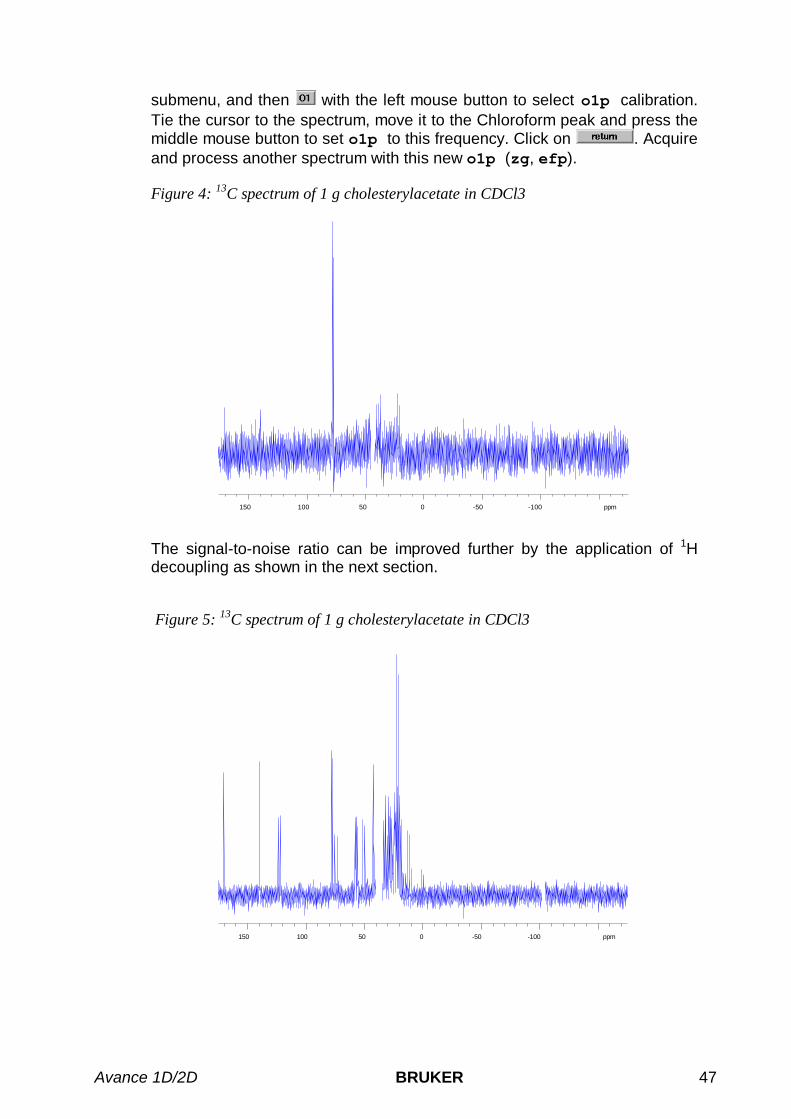
Avance 1D/2D BRUKER 47
submenu, and then with the left mouse button to select o1p calibration.Tie the cursor to the spectrum, move it to the Chloroform peak and press themiddle mouse button to set o1p to this frequency. Click on . Acquireand process another spectrum with this new o1p (zg, efp).
Figure 4: 13C spectrum of 1 g cholesterylacetate in CDCl3
150 100 50 0 -50 -100 ppm
The signal-to-noise ratio can be improved further by the application of 1Hdecoupling as shown in the next section.
Figure 5: 13C spectrum of 1 g cholesterylacetate in CDCl3
150 100 50 0 -50 -100 ppm

48 BRUKER Avance 1D/2D
5.3 One-Pulse Experiment with 1H Decoupling
The one-pulse sequence with 1H decoupling is shown in Figure 6. In additionto the one-pulse sequence used before, 1H is decoupled throughout theentire length of the pulse program.
Figure 6: 13C One-Pulse Sequence with 1H Decoupling
¦ d1 ¦ p1 acq
13C trd
π/2
1H decoupling
Before acquiring a 1H-decoupled 13C spectrum, the frequency of the 1Hsignals in must be determined. Figure 2 (Section 3.9) shows a 1H spectrumof cholesterylacetate (or look it up with re setup1h 1 1): Most 1H signalslie in the range of 0.5 to 5.5 ppm. An appropriate frequency for 1H decouplingwould therefore be 3 ppm. In general, 5 ppm is a safe frequency to select for1H decoupling if no 1H spectrum is available.
In case you looked up the 1H spectrum (data set proton/1/1), return to theprevious carbon spectrum by entering re setup13c 3 1. Enter edc, setEXPNO to 3 and click on SAVE to create the data set setup13c/3/1.
Enter eda and set the acquisition parameters as shown in Table 17.

Avance 1D/2D BRUKER 49
Table 17: 13C Acquisition Parameters for 1H Decoupled Spectrum
Parameter Value Comments
PULPROG zgdc see Figure 6 for pulse sequence diagram.
TD 32k
NS 1
DS 0
D1 2 should be 1–5*T1(13C).
P1 3 the default unit for pulse lengths is micro-seconds; entering “3” sets a pulse length of 3microseconds
PL1 power level for the p1 pulse (13C)
See also “Important note on power levels”
Pl12 low power level on F2 channel (1H) asdetermined in Section 4.2.6 for ROESY spinlock
PCPD2 1H 90° pulse for cpd sequence as determinedin Section 4.2.6
SW 350 ppm
O1P frequency of 13C carrier as optimized inSection 5.2
O2P 3 frequency of 1H carrier
CPDPRG2 waltz16 1H decoupling sequence
Enter zg to acquire an FID.
Enter efp to perform line broadening, Fourier transformation, and phasecorrection. A 1H decoupled 13C spectrum is shown in Figure 7. Note theimproved signal-to-noise ratio.

50 BRUKER Avance 1D/2D
Figure 7: 13C spectrum of 1 g cholesterylacetate in CDCl3 with 1H decoupling
200 150 100 50 0 -50 ppm

Avance 1D/2D BRUKER 51
6 Pulse Calibration: Carbon
6.1 Carbon Observe 90° Pulse
The 13C observe pulse calibration experiment requires a sample with a strong13C signal, e.g., 80% Benzene in Acetone-d6. If no appropriate sample isavailable, the inverse mode 13C pulse calibration procedure described inSection 6.3 can be used instead.
6.1.1 PreparationInsert the sample and lock the spectrometer (lock). Readjust the Z and Z2
shims until the lock level is maximal (use lockdisp). Tune and match theprobehead for 13C observation and 1H decoupling (see Chapter 2.5). Create anew data set: Enter re proton 1 1, enter edc and change the followingparameters:.
NAME test13cEXPNO 1PROCNO 1 .
Click on SAVE to create the data set test13c/1/1.
Enter edsp and set NUC1 to 13C, turn off NUC2 and press the DEFAULTbutton, then click on SAVE.
Enter eda and set the acquisition parameters as shown in Table 18.
Table 18: 1D 1H one-pulse Acquisition Parameters
Parameter Value Comments
PULPROG zg see Figure 1 for pulse sequence diagram.
TD 4 k
NS 1
DS 0
D1 20 interscan delay (20s, because of long T1)
P1 3 start with 3µs, which should correspond toless than a 90° pulse
PL1 power level for the p1 pulse
see “An Important Note on Power Levels” onpage 9
SW 350 start with a large spectral width of 350ppm;which will be optimized lateron
o1p start with 100ppm, it will be optimized later

52 BRUKER Avance 1D/2D
Enter rga to perform an automatic receiver gain adjustment; enter zg toacquire the FID, and edp to set the processing parameters as shown inTable 19.
Table 19: 1D 13C one-pulse Processing Parameters
Parameter Value Comments
SI 2 k
LB 3 Hz
PSCAL global
Add line broadening and Fourier transform the spectrum with the commandef. Manually phase correct the spectrum and store the correction.
Type sref to calibrate the spectrum and confirm the message “no peakfound in ‘sref' default calibration done”.
6.1.2 Optimize the Carrier Frequency and the Spectral WidthThe carrier frequency should now be set to the signal used to calibrate the90° pulse: Expand the spectrum until only the doublet at 130 ppm isdisplayed. Enter the calibration submenu by clicking . Click onwith the left mouse button and move the cursor to the center of the doublet.Click the middle mouse button to assign o1p to this frequency. Clickto exit the calibration submenu and return to the main window.
Reduce the spectral width by entering swh and change the value to 1000(Hz). Acquire and Fourier transform another spectrum (zg, ef).
6.1.3 Define the Phase Correction and the Plot RegionNow it is necessary to define the phase correction and spectral region thatwill be plotted in the output file produced by paropt. Phase correct thespectrum so that the doublet is positive. Expand the spectrum so that thedoublet covers approximately the central third of the screen. Click onwith the left mouse button and answer the three questions as follows:
F1 133 ppmF2 127 ppmchange y-scaling on display according to PSCAL? y
6.1.4 Calibration: High PowerAs for the 1H 90° calibration (Chapter 4.2.4), the automation program paroptis used. Type xau paropt and answer the questions as follows:
Enter parameter to modify: p1Enter initial parameter value: 2Enter parameter increment: 2Enter # of experiments: 16

Avance 1D/2D BRUKER 53
Paropt acquires and processes 16 spectra while incrementing the parameterp1 from 2 µsec to 32 µsec. The result is displayed side-by-side intest13c/1/999 and should resemble Figure 8. At the end of the experiment,the message “paropt finished” appears and a value for p1 is displayed, whichcorresponds to the 90° pulse length of the 13C transmitter using the currentpower level pl1. Write this value down and follow the procedure below toobtain a more accurate 90° pulse measurement.
Return to the data set test13c/1/1 by entering re 1 1. Type p1 and enter avalue corresponding to a 360° pulse (i.e., four times the 90° valuedetermined by paropt above). Acquire and process another spectrum (zg,efp). Change p1 slightly, acquire and process a spectrum again, until thedoublet shows a zero-crossing indicating the 360° pulse. The 360° pulse timedivided by 4 is the exact 90° pulse length for the 13C transmitter for the powerlevel pl1.
Note that the probe may arc, if the 90° pulse length is less than 5 µsec for5 mm probes and less than 10 µsec for 10 mm probes. In this case the pl1must be set to a higher value (increase the attenuation on the transmitter)and the corresponding 90° pulse length must be determined again.
Figure 8: Paropt Results for 13C 90° Pulse Calibration
p1 = 90°
p1 = 180°p1 = 270°

54 BRUKER Avance 1D/2D
6.2 Proton Decoupling 90° Pulse Dur ing 13C Acquisition
Ideally, this procedure is carried out immediately following the 13C observepulse calibration described above, since the magnet is then locked andshimmed, and the probehead is tuned and matched for both 13C and 1H.
6.2.1 SampleFor the 1H decoupling pulse calibration, the sample must yield a 13C signal ofreasonable intensity with a detectable scalar 13C–1H coupling: Therefore,80% Benzene in Acetone-d6 is a good choice.
6.2.2 Pulse SequenceThe pulse sequence used is called DECP90 and it is shown in Figure 9. Thesequence consists of a recycle delay (trd, d1) followed by a 90° 13C pulse(p1), a delay 1/[2J(13C,1H)] (d2, cnst2) for the evolution of antiphase 13C–1Hmagnetization, a 1H pulse (p3), and the 13C detection period (acq, aq). Forthe calibration of the 90° 1H decoupling pulse, the length (and/or the strength)of the 1H pulse p3 (and/or the power level pl2) is adjusted. No signal isacquired for an exact 1H 90° pulse p3, since only undetectable multiplequantum coherence 13C magnetization is present.
Figure 9: DECP90 Pulse Sequence
13C
1H
d1 p1 p3
π/2
1/[2J(13C,1H)]trd acq
d2
6.2.3 Set the 1H Carrier FrequencyThe first spectrum will be a 1H observe experiment to determine the correctfrequency for the DECP90 1H decoupling pulse. Create a new data setstarting from e.g., proton/1/1 (re proton 1 1), enter edc and change thefollowing parameters:
NAME testdecEXPNO 1PROCNO 1
Click on SAVE to create the data set testdec/1/1 and enter eda to set theacquisition parameters as shown in Table 20.

Avance 1D/2D BRUKER 55
Table 20: 1D 1H one-pulse Acquisition Parameters
Parameter Value Comments
PULPROG zg see Figure 1 for the pulse sequence diagram.
TD 4 k
NS 1
DS 0
D1 10 interscan delay (10s, because of long T1)
P1 3 start with 3µs, which should correspond toless than a 90° pulse
PL1 high power level on F1 channel (1H) asdetermined in Section 4.2.4
SW 20 start with a large spectral width of 20ppm;which will be optimized lateron
o1p 5
Enter rga, zg and edp to perform an automatic receiver gain adjustment,acquire an FID, and set the processing parameters as shown in Table 21.
Table 21: 1D 1H one-pulse Processing Parameters
Parameter Value Comments
SI 2 k
LB 1
PSCAL global
Type the command ef to perform line broadening and Fouriertransformation, and phase correct the spectrum. Type sref to calibrate thespectrum and confirm the message “no peak found in ‘sref' default calibrationdone”.
Click the left mouse button with the cursor placed in the spectral field of themain window. Move the cursor to the top of the Benzene peak at around7.3 ppm and note the exact ppm-value of the cursor position in the small“Info” window. Click the left mouse button to release the cursor from thespectrum.
6.2.4 Set the 13C Carrier Frequency and the Spectral WidthThese parameters were already determined for the data set test13c/1/1. Totransfer all the parameters from test13c/1/1 to the new data set, enter retest13c 1 1, enter edc and change the following parameters:
NAME testdecEXPNO 2PROCNO 1

56 BRUKER Avance 1D/2D
Click on SAVE to create the data set testdec/2/1.
Since now 1H decoupling is required, enter edsp and set NUC2 to 1H so thatthe spectrometer parameters are as follows:
NUC1 13CNUC2 1H(NUC3 off)
Enter eda and set the acquisition parameters values as shown in Table 22.The parameters o1p and swh should be set as used in test13c/1/1. Set o2pto the exact 1H offset frequency determined in the previous section (around7.3ppm). The DECP90 experiment will not work as described below unlessboth o1p and o2p are set correctly.
Table 22: DECP90 Acquisition Parameters
Parameter Value Comments
PULPROG decp90 see Figure 9 for pulse sequence diagram.
TD 4 k
NS 1
DS 0
PL1 high power level on F1 channel (13C) asdetermined in Section 6.1.4
PL2 high power level on F2 channel (1H) asdetermined in Section 4.2.4
P1 13C 90° pulse as determined in Section 6.1.4
P3 3 start with 3µs, which should correspond toless than a 90° pulse
D1 5 interscan delay (5s, because of long T1)
CNST2 160 Hz heteronuclear scalar J(13C,1H) coupling
D2 3.125 msec 1/[2J(13C,1H)]
(calculated automatically from cnst2 above)
SWH 1000 Hz
o1p 13C offset as determined in Section 6.1.2
o2p 1H offset as determined in Section 6.2.3
Enter zg to acquire the FID (the receiver gain should already be setappropriately), enter edp and verify the processing parameters as shown inTable 23.

Avance 1D/2D BRUKER 57
Table 23: DECP90 Processing Parameters
Parameter Value Comments
SI 2 k
LB 1 Hz
PSCAL global
Fourier transform the spectrum with line broadening by the command ef.Manually phase correct the spectrum so that the left peak is positive and theright peak is negative, and store the correction.
The spectrum is already calibrated if the current data set was created fromtest13c/1/1. Since paropt is not used here, neither the phase correction northe plot region have to be defined.
6.2.5 Calibration: High PowerThe 1H 90° decoupling pulse length should be close to the 1H 90° observepulse length for the same power level: Set p3 to the value found in Section4.2.4 and acquire and process a spectrum (zg, efp). If the 1H 90° pulse (p3)is less than 90°, the left peak will be positive and the right peak negative. Ifthe pulse angle is between 90° and 270°, the phase of the two peaks will beopposite. If the p3 pulse length corresponds to a 90° pulse, the signals showa zero-crossing as shown in Figure 10.

58 BRUKER Avance 1D/2D
Figure 10: 1H Decoupling 90° Pulse Calibration
133 131 129 127 ppm
p3 > 90°
p3 = 90 °
p3 < 90 °
6.2.6 Calibration: Low Power for WALTZ-16 DecouplingThe WALTZ-16 composite pulse decoupling (cpd) sequence requires a 1H90° decoupling pulse length of 80 to 100 µsec. Adjust pl2 and p3 todetermine the 90° pulse length in this range. Make use of the rule of thumb:90° pulse length approximately doubles for an additional 6 dB increase inattenuation.
Note that the parameters used by cpd sequences are pcpd2 for the 90°pulse length and pl12 for the decoupler power level, rather than p3 and pl2as used here.
6.3 Carbon Decoupler 90° Pulse (Inverse Mode)
This calibration procedure should yield approximately the same pulse lengthas for the 13C observe 90° pulse (Section 6.1.4). However, the methoddescribed here is more convenient because of the more sensitive 1Hdetection instead of 13C. In addition, the T1 of 1H is shorter than for 13C, whichallows the selection of shorter interscan delays.
6.3.1 SampleFor these so-called inverse experiments, the detected nucleus is 1H, but 13Csatellites must be visible. Therefore, a convenient sample is the 1HLineshape Sample (3% Chloroform in Acetone-d6 for frequencies between300 MHz and 500 MHz, and 1% Chloroform in Acetone-d6 for frequencies

Avance 1D/2D BRUKER 59
>600 MHz). Here the procedure is described for this readily availablestandard sample. However, use the “Pulse Calibration” sample containing0.1M 13C-methanol and 0.1M 15N-urea in DMSO-d6, if this is available.
The same DECP90 pulse sequence as used for the 1H 90° decoupling pulsedetermination in Section 6.2 is used here, except that the 1H and 13Cchannels are interchanged as shown in Figure 11.
Figure 11: DECP90 Pulse Sequence
13C
1H
d1 p1 p3
π/2
1/[2J(13C,1H)]trd acq
d2
π/2
6.3.2 PreparationInsert the sample, lock the spectrometer, readjust the Z and Z2 shims untilthe lock level is optimized, tune and match the probehead for 1H observationand 13C decoupling.
6.3.3 Set the 13C Carrier FrequencyFirst, a 13C observe experiment is recorded to determine the correct 13Ccarrier frequency (which is o1p here but will be o2p in the inverse calibrationexperiment).
Create a new data set starting from a previous 13C data set, e.g., carbon/1/1(re carbon 1 1), enter edc and change the following parameters:
NAME testinvEXPNO 1PROCNO 1
Click on SAVE to create the data set testinv/1/1. Type edsp and set theparameters as follows for observing 13C and decoupling 1H:
NUC1 13CNUC2 1H(NUC3 off)
Click on SAVE to save the spectrometer parameters and return to the mainwindow and enter eda to set the acquisition parameters as shown Table 24.

60 BRUKER Avance 1D/2D
Table 24: 1D 13C One-pulse Acquisition Parameters
Parameter Value Comments
PULPROG zgdc
TD 4 k
NS 1
DS 0
PL1 high power level on F1 channel (13C) asdetermined in Section 6.1.4
PL12 low power level on F2 channel (1H) for cpd asdetermined in Section 6.2.6
P1 3 start with less than a 90° pulse
PCPD2 1H 90° pulse for cpd sequence as determinedin Section 6.2.6
D1 5
SWH 1000
RG 4 k
o1p 77ppm Chloroform resonance
o2p 5
CPDPRG2 waltz16 cpd sequence for the 1H decoupling
Notice that the spectral width (swh) is much smaller than usually used for 13Cspectra, because only the chloroform signal must be recorded and o1p is setto almost the correct frequency in this data set.
Enter zg to acquire the FID. Enter edp and set the processing parameters asshown in Table 25.
Table 25: 1D 13C One-pulse Processing Parameters
Parameter Value Comments
SI 2 k
LB 1 Hz
PSCAL global
Fourier transform the data (ef) and phase the spectrum manually. Typesref to calibrate the spectrum and confirm the message “no peak found in ‘sref' default calibration done”.
Expand the spectrum until only the chloroform signal at 77 ppm is displayed.Enter the calibration submenu by clicking . Click on with theleft mouse button and move the cursor to the center of the signal. Click themiddle mouse button to assign o1p to this frequency. Click to exit

Avance 1D/2D BRUKER 61
the calibration submenu and return to the main window. This o1p value willbe the 13C o2p value for the DECP90 pulse sequence below.
6.3.4 Set the 1H Carrier Frequency and the Spectral WidthNow, a 1H observe experiment to determine the correct offset for 1H (o1p)must be recorded: Create a new 1H data set starting from a previous one,e.g., proton/1/1 (re proton 1 1). Enter edc and change the followingparameters:
NAME testinvEXPNO 2PROCNO 1
Click on SAVE to create the data set testinv/2/1, then enter eda and changethe acquisition parameters as shown in Table 26.

62 BRUKER Avance 1D/2D
Table 26: 1D 1H One-pulse Acquisition Parameters
Parameter Value Comments
PULPROG zg see Figure 1 for pulse sequence diagram.
TD 8 k
NS 1
DS 0
PL1 high power level on F1 channel (1H) asdetermined in Section 4.2.4
P1 3 1H pulse (less than a 90° pulse)
D1 5
SW 20 ppm
o1p 5
Enter rga to perform an automatic receiver gain adjustment, zg to acquirethe FID and edp to set the processing parameters as shown in Table 27.
Table 27: 1D 1H One-pulse Processing Parameters
Parameter Value Comments
SI 4k
LB 0.3 Hz
PSCAL global
Fourier transform the data (ef) and phase correct the spectrum. Type srefto calibrate the spectrum and confirm the message “no peak found in ‘sref'default calibration done”.
Expand the spectrum until only the chloroform signal at 7.2ppm is displayedand set the o1p value exactly on the methanol peak in the menu(follow the same procedure as described in Section 4.2.2). The spectral width(swh) can now be reduced to 1000 Hz.
6.3.5 Preparations for the Inverse Pulse CalibrationThe correct 1H and 13C frequencies have now been determined. Next, aDECP90 spectrum is acquired to determine the appropriate phase correctionvalues. Create a new data set by entering edc and change EXPNO to 3.Click SAVE to create the data set testinv/3/1.
Enable 13C decoupling by entering edsp and set the following spectrometerparameters:

Avance 1D/2D BRUKER 63
NUC1 1HNUC2 13CNUC3 off
Click on SAVE to save the spectrometer parameters and return to the mainwindow. Set o2p to the o1p value of the 13C determined in Section 6.3.3.
Enter eda and set the acquisition parameters as shown in Table 28.
Table 28: DECP90 Acquisition Parameters
Parameter Value Comments
PULPROG decp90 see Figure 11 for pulse sequence diagram.
TD 8 k
NS 1
DS 0
PL1 high power level on F1 channel (1H) asdetermined in Section 4.2.4
PL2 high power level on F2 channel (13C) asdetermined in Section 6.1.4
P1 1H 90° pulse as determined in Section 4.2.4
P3 0 for the phase correction, do not use p3
D1 5 relaxation delay; should be 1–5 * T1(1H).
CNST2 214 heteronuclear scalar J(13C,1H) coupling [Hz]
D2 3.34ms 1/[2J(13C,1H)]
(calculated automatically from cnst2 above)
SWH 1000 Hz
RG use value from testinv/2/1.
o1p ~7.24ppm 1H offset frequency of chloroform peak asdetermined in Section 6.3.4
o2p ~77ppm 13C offset frequency of chloroform peak asdetermined in Section 6.3.3
Enter zg to acquire the FID and enter edp to set the processing parametersas shown in Table 29.
Table 29: DECP90 Processing Parameters
Parameter Value Comments
SI 4 k
LB 0.3 Hz
PSCAL global

64 BRUKER Avance 1D/2D
Fourier transform the spectrum (ef). Expand the spectrum to display theregion between 8.5 to 7.5 ppm, in the region of the chloroform peak with it’stwo 13C satellites. Correct the phase in a way that the left satellite is positiveand the right satellite is negative.
6.3.6 Calibration: High PowerSet p3 to the value obtained with the direct method in Section 6.1. Acquireand process another spectrum (zg, efp). If the pulse is less than 90°, the leftsatellite will remain positive and the right satellite negative. If the pulse angleis between 90° and 270°, the two satellite signals will show opposite phase. Ifthe p3 pulse corresponds to 90°, the satellites show a zero-crossing (Figure12).
Figure 12: 13C Decouple 90° Pulse Calibration Results on the chloroform sample
8.5 8.3 8.1 7.9 7.7 ppm
p3 < 90°
p3 = 90°
p3 > 90°
6.3.7 Calibration: Low Power for GARP DecouplingThe GARP composite pulse decoupling (cpd) sequence requires a 90°decoupling pulse length of 60 to 70 µsec. Adjust pl2 and p3 to determinethe combination that yields a 90° pulse length in this range. Use the rule ofthumb: The pulse length doubles for a 6 dB increase in attenuation.

Avance 1D/2D BRUKER 65
Note that the parameters used by cpd sequences are pcpd2 for the 90°pulse length and pl12 for the decoupler power level, rather than p3 and pl2as used here.
6.4 1D Inverse Test Sequence
The 1D HMQC pulse sequence shown in Figure 13 is used to check theparameters for inverse experiments. This experiment detects only signals ofprotons directly attached to 13C nuclei, whereas the signal arising fromprotons attached to 12C is suppressed by phase cycling. Thus, the 1D HMQCspectrum of the current sample (10% Chloroform in Acetone-d6) yields onlysignal from the 13C satellites without the large central peak.
Figure 13: 1D HMQC Pulse Sequence
¦ d1 d2 d2 acq
1H trd
π/2 π
13C
π/2 π/2
1/(2JXH) 1/(2JXH)
p3 p3
p1 p2
Create a new data set starting from testinv/3/1 (re testinv 3 1), enteredc and set EXPNO to 4. Click SAVE to create the data set testinv/4/1. Entereda and set the acquisition parameters as shown in Table 30.

66 BRUKER Avance 1D/2D
Table 30: 1D HMQC Acquisition Parameters
Parameter Value Comments
PULPROG inv4ndrd1d see Figure 13 for pulse sequence diagram.
TD 8 k
NS 16 the number of scans should be 4 * n in orderfor the phase cycling to work properly.
DS 16 number of dummy scans.
PL1 high power level on F1 channel (1H) asdetermined in Section 4.2.4
PL2 high power level on F2 channel (13C) asdetermined in Section 6.1.4
P1 1H 90° pulse as determined in Section 4.2.4
P2 1H 180° pulse: set to 2*P1
P3 13C 90° pulse as determined in Section 6.3.6
D1 20 sec relaxation delay; should be 1–5 * T1(1H).
CNST2 214 heteronuclear scalar J(13C,1H) coupling [Hz]
Enter zg to acquire the FID and edp to set the processing parameters asshown in Table 31.
Table 31: 1D HMQC Processing Parameters
Parameter Value Comments
SI 4 k
WDW EM
LB 0.30 Hz
PKNL TRUE necessary when using the digital filter.
Fourier transform the data (ef) and phase correct the spectrum.
A 1D HMQC spectrum of Chloroform is shown in Figure 14. Note that thephase cycling is not as perfect to completely suppress the main signal arisingfrom 1H directly attached to 12C, due to technical limitations
.

Avance 1D/2D BRUKER 67
Figure 14: 1D HMQC Spectrum of Chloroform
8.7 8.5 8.3 8.1 7.9 7.7 7.5 ppm

68 BRUKER Avance 1D/2D

Avance 1D/2D BRUKER 69
7 Advanced 1D 13C Experiments
7.1 Carbon Experiments with Gated 1H-Decoupling
In principle, the values for scalar couplings between 1H and 13C, and thesignal multiplicity can give additional information for the structuredetermination. The disadvantages of not decoupling 1H in 13C spectra are thedecreased sensitivity due to the distribution of the signal intensity into thedifferent lines of the multiplet, the signal overlap, and the missing NOE effect.This chapter describes the acquisition and processing of 13C spectraacquired with commonly used 1H decoupling techniques called ‘gated-decoupling’ and ‘inverse gated-decoupling’.
The gated-decoupled 13C spectrum is recorded with 1H decoupling during therelaxation delay, whereas the decoupling is switched off during 13Cacquisition.
For the inverse gated-decoupling experiment the 1H decoupling is activeduring the acquisition, whereas it is switched off during the relaxation delay.The sensitivity improvement due to the NOE-effect is suppressed for thisexperiment and thus the acquired spectrum can be integrated. Note thatthere is a build up of the NOE-effect during the acquisition period whendecoupling is active. In order to suppress this NOE-effect the relaxation delaymust be 10-times the T1 relaxation time for 13C.
The pulse sequences for the gated-decoupling and the inverse gated-decoupling experiments are shown in Figure 15 and Figure 16, respectively.
However, before acquiring a 1H-decoupled 13C spectrum, the frequencies ofthe cholesterylacetate 1H signals must be determined. See Section 5.3 forthe determination of the exact 1H carrier frequency. As a rule of thumb,5 ppm is a safe frequency to select for 1H decoupling when no optimized 1Hspectrum is available.
Figure 15: 13C Pulse Sequence with Gated 1H Decoupling
¦ d1 ¦ p1 acq
13C trd
π/2
1H decoupling

70 BRUKER Avance 1D/2D
Return to the carbon/3/1 data set by entering re carbon 3 1. Enter edc andset EXPNO to 4. Click on to create the data set carbon/4/1 for the1H-gated-decoupled 13C spectrum.
Enter edsp and set NUC2 to 1H. Set o1p to the value determined from the1H spectrum or to 5 ppm. Enter eda and set the acquisition parameters asshown in Table 32.
Table 32: 13C Acquisition Parameters with Gated and Inverse Gated-1H Decoupling
Parameter Value Comments
PULPROG zggd
zgig
zggd for gated-decoupling
zgig for inverse gated-decoupling
TD 32 k
NS 16
DS 4
PL1 high power level on F1 channel (13C) asdetermined in Section 6.1.4
PL2 120 no high power pulses on F2 channel (1H)
PL12 low power level on F2 channel (1H) for CPDas determined in Section 6.2.6
D1 2
60
2s for gated-decoupling
60s for inverse gated-decoupling
P1 13C 90o pulse as determined in Section 6.1.4
SW 250 250 ppm
RG 8 k or use rga
o1p 120 frequency of the 13C carrier (120 ppm)
o2p frequency of the 1H carrier (see text)
PCPD2 1H 90o pulse for cpd sequence as determinedin Section 6.2.6
CPDPRG2 waltz16 1H decoupling sequence
Enter rga to start the automatic receiver gain adjustment and zg to acquirethe FID.
Enter si and set it to 32k, set lb to 3 and Fourier transform the data usingef. Phase correct the spectrum and store the correction.
The resulting spectrum is noisy compared to the regularly decoupled 13Cspectrum. The most intense peak arises from the Chloroform solvent, whichactually is a triplet.

Avance 1D/2D BRUKER 71
Figure 16: 13C Spectrum of 1g Cholesterylacetate in CDCl3 using (a) Gated-Decoupling, and
7.1.1 Plotting 1D 13C Spectra1D 13C spectra are most easily plotted using the standard plot parameter file,which sets most of the plotting parameters to appropriate values. Type rparand select standard1D from the list of parameter file names. Select plot

72 BRUKER Avance 1D/2D
from the menu of parameter file types. Equivalently, simply enter rparstandard1D plot.
To select the spectral region (full or expanded) to be plotted, make sure thespectrum appears on the screen as desired, and then type defplot. Hitreturn in response to the following three questions:
F1 = <return>F2 = <return>Change y-scaling on display according to PSCAL? <return>
Unless special precautions are taken to deal with the long 13C T1 relaxationtimes and potential NOE build-up during 1H decoupling, the integratedintensities in 1D 13C-NMR spectra do not reflect the correct numbers ofdifferent types of 13C nuclei in a given molecule. Thus, standard 13C spectraare usually not integrated and the integrals are therefore not plotted: Typeedg and click the button next to the parameter INTEGR so that it toggles tono. Click to exit the edg menu.
Finally, create a title for the spectrum by entering setti and write a title.Save the file and simply enter plot (provided the correct plotter is selectedin edo) to plot the spectrum.
7.2 DEPT
DEPT (Distortionless Enhancement by Polarization Transfer) is a polarizationtransfer technique used for the observation of nuclei with a smallgyromagnetic ratio, which are J-coupled to 1H (most commonly 13C). DEPT isa spectral editing sequence, that is, it can be used to generate separate 13Csubspectra for methyl (CH3), methylene (CH2), and methine (CH) signals.DEPT makes use of the generation and manipulation of multiple quantumcoherences to differentiate between the different types of 13C signals.Quaternary carbons are missing from DEPT spectra because the large one-bond heteronuclear J-coupling (JXH) is used for polarization transfer.
DEPT may be run with or without 1H-decoupling and it is relatively insensitiveto the precise matching of delays with coupling constants, and so is mucheasier to use than the closely related INEPT sequence. DEPT, on the otherhand, is more sensitive to pulse imperfections than INEPT.
The sample used in this chapter is 1 g Cholesterylacetate in CDCl3.

Avance 1D/2D BRUKER 73
The DEPT pulse sequence is shown in Figure 17. The final 1H pulse with flipangle α selects for the CH3, CH2 or CH signals. This angle is set to 45° in theDEPT-45 sequence, which yields spectra with positive CH, CH2, and CH3signals; to 90° in DEPT-90, which yields spectra with only CH signals; and to135° in DEPT-135, which yields spectra with positive CH and CH3 signalsand negative CH2 signals.
Figure 17: DEPT Pulse Sequence
7.2.1 Acquisition and ProcessingInsert the sample in the magnet. Lock the spectrometer. Readjust the Z andZ2 shims until the lock level is optimized. Tune and match the probehead for13C observation and 1H decoupling.
7.2.2 Reference SpectraSince DEPT is a 13C-observe experiment with 1H-decoupling experiment, areference 1H spectrum of the sample must be recorded to determine thecorrect o2p for 1H decoupling. Then, a 1H-decoupled 13C spectrum must berecorded to determine the correct o1p and sw for the DEPT experiments.However, both steps were already carried out in Section 5.3 (a 1H-decoupled13C reference spectrum of this sample can be found in carbon/3/1).
7.2.3 Create a New Data SetEnter re carbon 3 1 to call up the reference spectrum. Enter edc andchange the following parameters:
NAME deptEXPNO 1PROCNO 1
Click to create the data set dept/1/1.
¦ d1 d2 d2 d2 acq
13C trd
π/2 π
1H
π/2 π α
1/(2JXH) 1/(2JXH)
p3 p4 p0
p1 p2
1/(2JXH) cpd
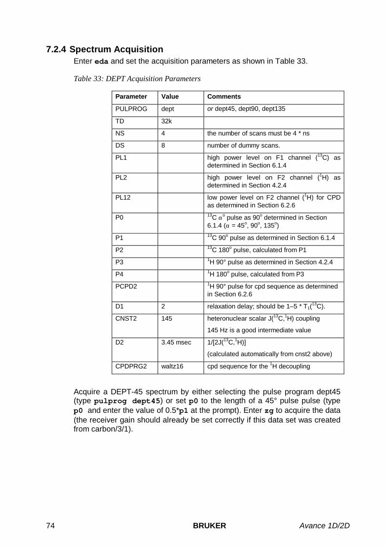
74 BRUKER Avance 1D/2D
7.2.4 Spectrum AcquisitionEnter eda and set the acquisition parameters as shown in Table 33.
Table 33: DEPT Acquisition Parameters
Parameter Value Comments
PULPROG dept or dept45, dept90, dept135
TD 32k
NS 4 the number of scans must be 4 * ns
DS 8 number of dummy scans.
PL1 high power level on F1 channel (13C) asdetermined in Section 6.1.4
PL2 high power level on F2 channel (1H) asdetermined in Section 4.2.4
PL12 low power level on F2 channel (1H) for CPDas determined in Section 6.2.6
P0 13C αo pulse as 90o determined in Section6.1.4 (α = 45o, 90o, 135o)
P1 13C 90o pulse as determined in Section 6.1.4
P2 13C 180o pulse, calculated from P1
P3 1H 90° pulse as determined in Section 4.2.4
P4 1H 180o pulse, calculated from P3
PCPD2 1H 90° pulse for cpd sequence as determinedin Section 6.2.6
D1 2 relaxation delay; should be 1–5 * T1(13C).
CNST2 145 heteronuclear scalar J(13C,1H) coupling
145 Hz is a good intermediate value
D2 3.45 msec 1/[2J(13C,1H)]
(calculated automatically from cnst2 above)
CPDPRG2 waltz16 cpd sequence for the 1H decoupling
Acquire a DEPT-45 spectrum by either selecting the pulse program dept45(type pulprog dept45) or set p0 to the length of a 45° pulse pulse (typep0 and enter the value of 0.5*p1 at the prompt). Enter zg to acquire the data(the receiver gain should already be set correctly if this data set was createdfrom carbon/3/1).

Avance 1D/2D BRUKER 75
7.2.5 Processing of the SpectrumEnter edp and set the processing parameters as shown in Table 34.
Table 34: DEPT Processing Parameters
Parameter Value Comments
SI 16k
WDW EM exponential multiplication
LB 2 2 Hz line broadening.
PKNL TRUE necessary when using the digital filter
Add line broadening and Fourier transform the time domain data with thecommand ef. Manually phase correct the spectrum so that all peaks arepositive. The signals in this spectrum arise from the 13C nuclei in CH, CH2,and CH3 groups.
7.2.6 Other spectraTo obtain a DEPT-90 spectrum create the data set dept/2/1 and either selectthe pulse program dept90 (type pulprog dept90) or set p0 to the length ofa 90° pulse (type p0 and enter the value of p1 at the prompt). Acquire (zg)and process (efp) the data. Only signals from CH groups are visible in thisexperiment.
To obtain a DEPT-135 spectrum, create the data set dept/3/1 and eitherselect the pulse program dept135 (type pulprog dept135) or set p0 to thelength of a 135° pulse (type p0 and enter the value of 1.5*p1 at the prompt).Acquire (zg) and process (efp) the data. Only signals from CH and CH3
groups are visible in this experiment.
7.2.7 Plot the spectraSee Section 7.1.1 for instructions on how to plot the acquired spectra. DEPT-45, DEPT-90, and DEPT-135 spectra of 1 g Cholesterylacetate in CDCl3 areshown in Figure 18.
The DEPT results can be compared with the standard 1H-decoupled 13Cspectrum in carbon/3/1 (see Section 5.3). Note that the signals from thequaternary 13C in the carbon/3/1 do not appear in any of the DEPT spectra.From the combination of standard 1H-decoupled, and DEPT-45, -90, and -135 spectra, it is possible to determine which signals arise from primary,secondary, tertiary, and quaternary 13C's.

76 BRUKER Avance 1D/2D
Figure 18: DEPT Spectra of 1 g Cholesterylacetate in CDCl3
120 100 80 60 40 20 0 ppm
DEPT-45
DEPT-90
DEPT-135

Avance 1D/2D BRUKER 77
7.3 APT (Attached Proton Test)
The APT (Attached Proton Test) is a simple experiment for assigningmultiplicities in 13C NMR spectroscopy. The APT pulse sequence is shown inFigure 19. The first 90 degree pulse creates transverse magnetisationfollowed by a 180 degree pulse in the middle of the evolution period (spinecho sequence). During the evolution period the different components of thecarbon multiplets precess at their individual frequencies. During the half ofthe evolution period the decoupler is OFF to introduce J-modulation in thespectrum. The length of the evolution period controls the amplitude of thecarbon signal. Normally the evolution period is set to 1/(JCH) then the CH andCH3 groups appear as positive peaks while those from CH2 and quarternarycarbons are negative. Compared to the DEPT experiment all carbon nucleiare visible in one spectrum.
Figure 19: APT Pulse Sequence
H1
C13
CPD CPD
1/(J )XH 1/(J )XH
d1 d20 d20 acq p1 p2
ππ/2
References: D.W. Brown, T.T. Nakashima, and D.L. Rabenstein, J. Magn.Res., 45, 302 (1981); S.L. Patt and N. Shoorly, J. Magn. Reson., 46, 535(1982); A.M. Torres, T. T. Nakashima, and R.E.D. McClung, J. Magn.Reson., 101, 285 (1993).
7.3.1 Acquisition and ProcessingInsert the sample in the magnet. Lock the spectrometer. Readjust the Z andZ2 shims until the lock level is optimized. Tune and match the probehead for13C observation and 1H decoupling.
7.3.2 Reference SpectraSince APT is a 13C-observe experiment with 1H-decoupling, a reference 1Hspectrum of the sample must be recorded to determine the correct o2p for 1H

78 BRUKER Avance 1D/2D
decoupling. Then, a 1H-decoupled 13C spectrum must be recorded todetermine the correct o1p and sw for the APT experiments. However, bothsteps were already carried out in Section 5.3 (a 1H-decoupled 13C referencespectrum of this sample can be found in carbon/3/1).
7.3.3 Create a New Data SetEnter re carbon 3 1 to call up the reference spectrum. Enter edc andchange the following parameters:
NAME aptEXPNO 1PROCNO 1
Click to create the data set apt/1/1.
7.3.4 Spectrum AcquisitionEnter eda and set the acquisition parameters as shown in Table 35.
Table 35: APT Acquisition Parameters
Parameter Value Comments
PULPROG jmod spin echo experiment
TD 32k
NS 4 the number of scans must be 4 * ns
DS 4 number of dummy scans.
PL1 high power level on F1 channel (13C) asdetermined in Section 6.1.4
PL2 high power level on F2 channel (1H) asdetermined in Section 4.2.4
PL12 low power level on F2 channel (1H) for CPDas determined in Section 6.2.6
P1 13C pulse as 90o determined in Section 6.1.4
P2 13C 180o pulse, calculated from P1
PCPD2 1H 90° pulse for cpd sequence as determinedin Section 6.2.6
D1 2 relaxation delay; should be 1–5 * T1(13C).
CNST2 140 heteronuclear scalar J(13C,1H) coupling
140 Hz is a good intermediate value
CNST11 1
2
X, XH2 positive, XH, XH3 negative
only X
D20 7.14 msec 1/[1J(13C,1H)]
(calculated automatically from cnst2 * cnst11above)
CPDPRG2 waltz16 cpd sequence for the 1H decoupling

Avance 1D/2D BRUKER 79
7.3.5 Processing of the SpectrumEnter edp and set the processing parameters as shown in Table 36.
Table 36: APT Processing Parameters
Parameter Value Comments
SI 16k
WDW EM exponential multiplication
LB 2 2 Hz line broadening.
PKNL TRUE necessary when using the digital filter
Add line broadening and Fourier transform the time domain data with thecommand ef. Manually phase correct the spectrum so that CH and CH3
groups are positive and C and CH2 groups are negative..
.
7.3.6 Plot the spectraSee Section 7.1.1 for instructions on how to plot the acquired spectra. TheAPT spectrum of 1 g Cholesterylacetate in CDCl3 is shown in Figure20.
The APT results can be compared with the standard 1H-decoupled 13Cspectrum in carbon/3/1 (see Section 5.3) and with the DEPT experiments.Note that the signals from the quaternary 13C is visible in the APTexperiment.
Figure 20: APT Spectrum of 1 g Cholesterylacetate in CDCl3

80 BRUKER Avance 1D/2D

Avance 1D/2D BRUKER 81
8 COSY
8.1 Introduction
COSY (COrrelation SpectroscopY) is a homonuclear 2D technique that isused to correlate the chemical shifts of 1H nuclei which are J-coupled to oneanother. In this chapter, two types of COSY sequences, magnitude COSYand double-quantum filtered DQF-COSY with and without pulsed fieldgradients, will be discussed. The different pulse sequences are quite simpleand can be explained as follows: The first pulse creates transversemagnetization components which evolve chemical shift and homonuclear J-coupling during the evolution period t1. The second pulse mixes themagnetization components among all the transitions that belong to the samecoupled spin systems. The final distribution of labeled magnetizationcomponents is detected by measuring their precession frequencies duringthe detection period t2. The COSY spectrum is processed by a 2D Fouriertransform with respect to t1 and t2, and the cross peaks indicate which 1Hnuclei are J-coupled.
The sample used to demonstrate magnitude and DQF-COSY in this chapteris 50 mM Cyclosporin in benzene-d6.
8.2 Magnitude COSY
Several simple two-pulse programs can be used to record a magnitude modeCOSY spectrum, e.g., cosy, cosy45, and cosy90. These vary with respect tothe angle of the final pulse. Any value between 20o and 90o may be chosenfor the final pulse angle. However, a pulse angle of 45o is recommendedbecause this yields the best signal-to-noise ratio together with a simple crosspeak structure in the final spectrum.
The signals acquired with one of these experiments have absorptive anddispersive lineshape contributions in both F1 and F2 dimensions. This meansthat it is impossible to phase the spectrum with all peaks purely absorptive,and, as a consequence, the spectrum must be displayed in magnitude mode.A typical spectral resolution of 3 Hz/pt is sufficient for resolving large scalarcouplings. In order to resolve small J-couplings fine digital resolution isrequired, which significantly increases the experimental time. In general, theDQF-COSY experiment is recommended if a higher resolution is desired.
References: W. P. Aue, E. Bartholdi, and R. R. Ernst, J. Chem. Phys., 64,2229 (1976); K. Nagayama, A. Kumar, K. Wüthrich, and R. R. Ernst, J. Magn.Reson., 40, 321 (1980).

82 BRUKER Avance 1D/2D
8.2.1 Pulse SequenceThe COSY-45 pulse sequence is shown in Figure 21. The pulse p1 must beset to the appropriate 90o pulse length found in Chapter 4.2.4
Figure 21: COSY-45 Pulse Sequence
¦ d1 ¦ p1 p1 acq
1H trd t1
π/2 π/4
d0
8.2.2 Acquisition of the 2D COSY SpectrumInsert the sample in the magnet. Lock the spectrometer. Readjust the Z andZ2 shims until the lock level is optimized. Tune and match the probehead for1H observation.
It is recommended to run all 2D experiments without sample spinning.
Record a 1H reference spectrum to obtain the correct carrier frequency (o1p)and spectral width (sw) values: Enter re proton 1 1 to call up the data setproton/1/1; enter edc and change the following parameters
NAME cosyEXPNO 1PROCNO 1
Click to create the data set cosy/1/1.
Enter rga to perform an automatic receiver gain adjustment. Acquire andprocess a standard 1H spectrum. Calibrate the spectrum, and optimize swand o1p so that the 1H signals cover almost the entire spectral width. Acquirean optimized spectrum.
Type xau iexpno (increment experiment number) to create the data setcosy/2/1.
Enter eda and set PARMODE to 2D. Click on and ok the message “Delete ‘meta.ext' files?”. The window now switches to a 2D display and themessage “NEW 2D DATA SET” appears.
Enter eda and set the acquisition parameters as shown in Table 37. The F2parameters o1p and sw should be identical to the values used in theoptimized 1H reference spectrum (cosy/1/1). Note that in0 and sw(F1) arenot independent from each other.
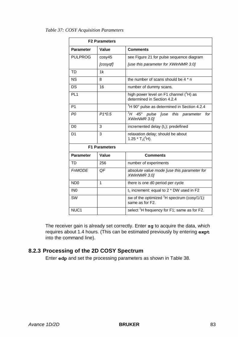
Avance 1D/2D BRUKER 83
Table 37: COSY Acquisition Parameters
F2 Parameters
Parameter Value Comments
PULPROG cosy45
[cosyqf]
see Figure 21 for pulse sequence diagram
[use this parameter for XWinNMR 3.0]
TD 1k
NS 8 the number of scans should be 4 * n
DS 16 number of dummy scans.
PL1 high power level on F1 channel (1H) asdetermined in Section 4.2.4
P1 1H 90° pulse as determined in Section 4.2.4
P0 P1*0.5 1H 45° pulse [use this parameter forXWinNMR 3.0]
D0 3 incremented delay (t1); predefined
D1 3 relaxation delay; should be about1.25 * T1(
1H).
F1 Parameters
Parameter Value Comments
TD 256 number of experiments
FnMODE QF absolute value mode [use this parameter forXWinNMR 3.0]
ND0 1 there is one d0 period per cycle
IN0 t1 increment: equal to 2 * DW used in F2
SW sw of the optimized 1H spectrum (cosy/1/1):same as for F2.
NUC1 select 1H frequency for F1; same as for F2.
The receiver gain is already set correctly. Enter zg to acquire the data, whichrequires about 1.4 hours. (This can be estimated previously by entering exptinto the command line).
8.2.3 Processing of the 2D COSY SpectrumEnter edp and set the processing parameters as shown in Table 38.

84 BRUKER Avance 1D/2D
Table 38: COSY Processing Parameters
F2 Parameters
Parameter Value Comments
SI 512
SF spectrum reference frequency (1H)
WDW SINE multiply data by phase-shifted sine function
SSB 0 choose pure sine wave
PH_mod no this is a magnitude spectrum
PKNL TRUE necessary when using the digital filter
BC_mod quad
F1 Parameters
Parameter Value Comments
SI 512
SF spectrum reference frequency (1H)
WDW SINE multiply data by phase-shifted sine function.
SSB 0 choose pure sine wave
PH_mod mc this is a magnitude spectrum
BC_mod no
MC2 QF determines type of FT in F1; QF results in aforward quadrature complex FT
Enter xfb to perform the 2D Fourier transformation.
For the magnitude COSY, sine-type window functions are selected tosuppress the diagonal peaks relative to the cross peaks. Such a windowfunction is also resolution enhancing, which is appropriate for a magnitudemode 2D spectrum. Adjust the threshold level by placing the cursor on the
button, holding down the left mouse button and moving the mouse upand down.
Since this is a magnitude spectrum, click on with the left mousebutton until only the positive peaks are displayed.
The region can be expanded with the button followed by choosing thedesired spectral region with the left mouse button depressed. The fullspectrum is displayed again by clicking the button.
The optimum may be saved by clicking on and confirming theappearing questions as follows
Change levels? yPlease enter number of positive levels? 6Display contours? n

Avance 1D/2D BRUKER 85
8.2.4 Plotting the SpectrumRead in the plot parameter file standard2D (rpar standard2D plot), whichsets most of the plotting parameters to appropriate values.
Enter edg to edit the plotting parameters: Click the ed next to the parameterEDPROJ1 to enter the F1 projection parameters submenu. Edit theparameters as follows:
PF1DU uPF1USER (name of user for file cosy/1/1)PF1NAME cosyPF1EXP 1PF1PROC 1
Click to save these changes and return to the edg menu.
Click the ed next to the parameter EDPROJ2 to enter the F2 projectionparameters submenu. Edit the parameters as follows:
PF2DU uPF2USER (name of user for file cosy/1/1)PF2NAME cosyPF2EXP 1PF2PROC 1 .
Click to save these changes and return to the edg menu, and againto exit the edg menu.
Create a title for the spectrum (setti) and plot the spectrum (plot). Amagnitude COSY spectrum of 50 mM Cyclosporin in C6D6 is shown in Figure20.
Figure 22: COSY Spectrum of 50 mM Cyclosporin in C6D6

86 BRUKER Avance 1D/2D
8.3 Double-Quantum Filtered (DQF) COSY
The DQF-COSY pulse sequence consists of three pulses, where the thirdpulse converts part of the multiple quantum coherence into observablesingle-quantum coherence, which is detected during the acquisition period.
One advantage of the DQF-COSY experiment is the phase-sensitivity, i.e.,the cross peaks can be displayed with pure absorption lineshapes in both theF1 and the F2 dimension. In general, a phase-sensitive spectrum has ahigher resolution than an otherwise equivalent magnitude spectrum becausethe magnitude lineshape is broader than the pure absorption lineshape.
Another advantage is the partial cancellation of the diagonal peaks in a DQF-COSY spectrum: Thus, the diagonal ridge is much less pronounced in aDQF-COSY spectrum than in a normal COSY spectrum.
A third advantage of the double quantum filter is the elimination of strongsignals, e.g., the solvent 1H which do not experience homonuclear J-coupling.
References: M. Rance, O. W. Sørensen, G. Bodenhausen, G. Wagner, R.R. Ernst, and K. Wüthrich, Biochem. Biophys. Res. Commun., 117, 479(1984); A. Derome and M. Williamson, J. Magn. Reson., 88, 117 (1990).
8.3.1 Pulse SequenceThe DQF-COSY pulse sequence is shown in Figure 23. The pulse p1 mustbe set to the appropriate 90o pulse length found in Chapter 4.2.4. Note thatthe DQF-COSY experiment is sensitive to high pulse-repetition rates, i.e., it isimportant to choose a long recycle delay time d1 in order to avoid multiple-quantum artifacts in the spectrum. A suitable value for this sample is d1 =3 sec.
Figure 23: DQF-COSY Pulse Sequence
¦ d1 ¦ p1 p1 p1 acq
1H trd t1
π/2 π/2 π/2
d0
8.3.2 Acquisition and ProcessingFrom the data set cosy/2/1, enter edc and change EXPNO to 3.
Click to create the data set cosy/3/1.
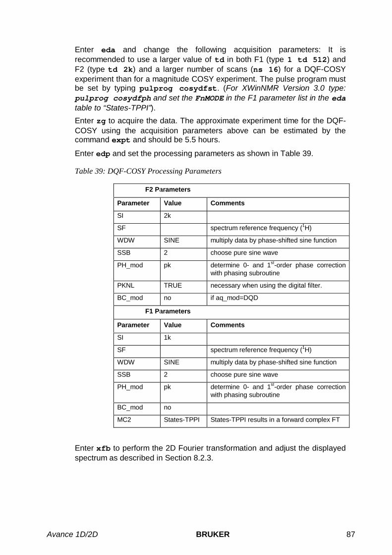
Avance 1D/2D BRUKER 87
Enter eda and change the following acquisition parameters: It isrecommended to use a larger value of td in both F1 (type 1 td 512) andF2 (type td 2k) and a larger number of scans (ns 16) for a DQF-COSYexperiment than for a magnitude COSY experiment. The pulse program mustbe set by typing pulprog cosydfst. (For XWinNMR Version 3.0 type:pulprog cosydfph and set the FnMODE in the F1 parameter list in the edatable to “States-TPPI”).
Enter zg to acquire the data. The approximate experiment time for the DQF-COSY using the acquisition parameters above can be estimated by thecommand expt and should be 5.5 hours.
Enter edp and set the processing parameters as shown in Table 39.
Table 39: DQF-COSY Processing Parameters
F2 Parameters
Parameter Value Comments
SI 2k
SF spectrum reference frequency (1H)
WDW SINE multiply data by phase-shifted sine function
SSB 2 choose pure sine wave
PH_mod pk determine 0- and 1st-order phase correctionwith phasing subroutine
PKNL TRUE necessary when using the digital filter.
BC_mod no if aq_mod=DQD
F1 Parameters
Parameter Value Comments
SI 1k
SF spectrum reference frequency (1H)
WDW SINE multiply data by phase-shifted sine function
SSB 2 choose pure sine wave
PH_mod pk determine 0- and 1st-order phase correctionwith phasing subroutine
BC_mod no
MC2 States-TPPI States-TPPI results in a forward complex FT
Enter xfb to perform the 2D Fourier transformation and adjust the displayedspectrum as described in Section 8.2.3.

88 BRUKER Avance 1D/2D
8.3.3 Phase correct the spectrumThe phase correction of DQF-COSY spectra is best performed whileexamining the cross peaks rather than the diagonal peaks. When thespectrum is phased properly, the cross peaks will be purely absorptive (i.e.,they will not have the slowly decaying wings characteristic of dispersionpeaks). However, since DQF-COSY peaks are antiphase (i.e., each multiplethas adjacent positive and negative peaks), it is not possible to phase thespectrum so that all peaks are positive.
Generally, a 2D spectrum is first phase corrected in the F2 dimension (rows),and then in the F1 dimension (columns). To phase correct the spectrum inF2, three rows each with a cross peak should be selected. The cross peak ofone row should be to the far left of the spectrum, the cross peak of thesecond row should be close to the middle, and the one of the third rowshould be to the far right of the spectrum.
Enter the phase correction menu by clicking on the button. Selectone row by clicking on with the left mouse button to tie the cursor tothe 2D spectrum appearing in the upper left corner of the display. Move themouse until the horizontal cross hair is aligned with a row that has a crosspeak. Select the row by clicking the middle mouse button. If the selected rowdoes not intersect the most intense portion of the cross peak, click
with the left mouse button until it does. Once the desired row is selected,click on with the left mouse button to move the row to window 1appearing in the upper right hand corner of the display.
Repeat the selection of rows described above for a row with a cross peak inthe middle and another row with a cross peak at the right edge of thespectrum and move them to window 2 and 3, respectively.
Now that three rows have been selected, the 0th- and 1st-order phasecorrections in F2 are determined by hand exactly as described for the 1Dspectrum in Section 3.8:
Click on the or the button to tie the cursor to the biggestpeak of the row in window 1. Phase Correct this row using the 0th-orderphase correction button . Correct the 1st-order phase correctionfor the other two rows using the button and observe the rows in window2 and 3, respectively.
Save the phase correction by returning to the main window (select Save &return at the prompt).
To phase correct the spectrum in F1, repeat the above procedure byselecting three columns rather than rows.
8.3.4 Plot the spectrumSee the plotting instructions given for the magnitude COSY spectrum inSection 8.2.4.
A DQF-COSY spectrum of 50 mM cyclosporin in C6D6 is shown in Figure 24.

Avance 1D/2D BRUKER 89
Figure 24: DQF-COSY Spectrum of 50 mM Cyclosporin in C6D6
8.4 Double-Quantum Filtered COSY using Pulsed FieldGradients (GRASP-DQF-COSY)
The first high-resolution NMR experiments using pulsed field gradients (PFG)were the COSY experiments mainly to demonstrate that the application ofPFGs can replace phase cycling. The quality in selecting a desiredcoherence pathway by PFGs turned out to be more efficient than phasecycling. In contrast to phase cycling, which requires several scans for each t1increment for coherence selection, field gradients allow coherence selectionwith only a single scan for each t1 increment.
There are mainly two common PFG applications with COSY experiments:
1. Quadrature detection in the ω1 dimension. The experiment time for such aCOSY is in the order of a few minutes.
2. Double-quantum filter: the quality of the double-quantum filter using fieldgradients is very efficient. Therefore, solvent signals without homonuclear1H coupling (like water) can be suppressed very efficiently withoutadditional solvent suppression techniques.
In this chapter we will describe the phase-sensitive double-quantum filteredCOSY experiment and the pulse sequence is shown in Figure 25.

90 BRUKER Avance 1D/2D
8.4.1 Pulse SequenceThe GRASP-DQF-COSY pulse sequence is very similar to the conventionalDQF-COSY pulse program. After the second pulse, the spin system exhibitsmultiple-quantum coherence and the application of a PFG G1 yields completedephasing of all coherences. In order to obtain a phase sensitive spectrumlater on, the effect of chemical shift evolution during G1 has to be eliminatedby a spin echo. The third 90o pulse converts part of the multiple quantumcoherence into observable single-quantum coherence, which is rephased bythe PFG G2 of proper intensity. All the unwanted magnetization staysdephased and can not be observed during the acquisition: Only spins J-coupled to at least one other spin are detected and solvent signals,especially water, are suppressed very efficiently.
The intensity ratio of the PFGs G1:G2 is 2: 1 for a double-quantum filter, and3:1 for a triple quantum filter:
Figure 25: GRASP-DQF-COSY Pulse Sequence
¦ ¦ p1 p1 p2 p1 p2 acq
1H trd t1
π/2 π/2 π π/2 π
d0d1
G 1 G2
Gradient
8.4.2 Acquisition and ProcessingFollow the instructions given in Sections 8.3.2 to 8.3.4 for the conventionalDQF-COSY and create the data set cosy/4/1 starting out from the DQF-COSY data set (cosy/3/1).
Three parameters related to the PFGs G1 and G2 must be defined: Thelength of the PFG (p16), the recovery delay after the PFG (d16), and theshape and the intensity of the individual gradients.
Table 40: GRASP DQF-COSY Acquisition Parameters
F2 Parameters
Parameter Value Comments
PULPROG cosygpmftp
cosygpmfph [use this parameter for XWinNMR 3.0]
TD 2K
NS 4
DS 16
PL1 high power level on F1 channel (1H) as
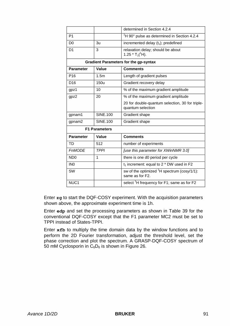
Avance 1D/2D BRUKER 91
determined in Section 4.2.4
P1 1H 90° pulse as determined in Section 4.2.4
D0 3u incremented delay (t1); predefined
D1 3 relaxation delay; should be about1.25 * T1(
1H).
Gradient Parameters for the gp-syntax
Parameter Value Comments
P16 1.5m Length of gradient pulses
D16 150u Gradient recovery delay
gpz1 10 % of the maximum gradient amplitude
gpz2 20 % of the maximum gradient amplitude
20 for double-quantum selection, 30 for triple-quantum selection
gpnam1 SINE.100 Gradient shape
gpnam2 SINE.100 Gradient shape
F1 Parameters
Parameter Value Comments
TD 512 number of experiments
FnMODE TPPI [use this parameter for XWinNMR 3.0]
ND0 1 there is one d0 period per cycle
IN0 t1 increment: equal to 2 * DW used in F2
SW sw of the optimized 1H spectrum (cosy/1/1):same as for F2.
NUC1 select 1H frequency for F1; same as for F2
Enter zg to start the DQF-COSY experiment. With the acquisition parametersshown above, the approximate experiment time is 1h.
Enter edp and set the processing parameters as shown in Table 39 for theconventional DQF-COSY except that the F1 parameter MC2 must be set toTPPI instead of States-TPPI.
Enter xfb to multiply the time domain data by the window functions and toperform the 2D Fourier transformation, adjust the threshold level, set thephase correction and plot the spectrum. A GRASP-DQF-COSY spectrum of50 mM Cyclosporin in C6D6 is shown in Figure 26.

92 BRUKER Avance 1D/2D
Figure 26: GRASP-DQF-COSY experiment of 50mM Cyclosporin in C6D6

Avance 1D/2D BRUKER 93
9 TOCSY
9.1 Introduction
TOCSY (TOtal Correlation SpectroscopY) provides a different mechanism ofcoherence transfer than COSY for 2D correlation spectroscopy in liquids. InTOCSY, cross peaks are generated between all members of a coupled spinnetwork. An advantage is that pure absorption mode spectra with positiveintensity peaks are created. In traditional COSY, cross peaks have zerointegrated intensity and the coherence transfer is restricted to directly spin-coupled nuclei. In TOCSY, oscillatory exchange is established whichproceeds through the entire coupling network so that there can be netmagnetization transfer from one spin to another even without direct coupling.The isotropic mixing which occurs during the spin-lock period of the TOCSYsequence exchanges all in-phase as well as antiphase coherences.
The coherence transfer period of the TOCSY sequence occurs during amultiple-pulse spin-lock period. The multiple-pulse spin-lock sequence mostcommonly used is MLEV-17. The length of the spin-lock period determineshow far the spin coupling network will be probed. A general rule of thumb isthat 1/(10 JHH) should be allowed for each transfer step, and five transfersteps are typically desired for the TOCSY spectrum.
The sample used to demonstrate TOCSY in this chapter is 50 mMCyclosporin in C6D6.
References: L. Braunschweiler and R. R. Ernst, J. Magn. Reson., 53, 521(1983); A. Bax and D. G. Davis, J. Magn. Reson., 65, 355 (1985).
The TOCSY pulse sequence is shown in Figure 27. The pulse p1 must beset to the appropriate 90° time found Section 4.2.4 and the MLEV-17sequence used during the spinlock period requires the calibrated 90° time p6as determined in Section 4.2.5.
Figure 27: TOCSY Pulse Sequence
1H trd t1 trim MLEV-17 trim
π/2
p11 p17 p5,p6,p7 p17
d1 d0

94 BRUKER Avance 1D/2D
9.2 Acquisition
Insert the sample in the magnet. Lock the spectrometer. Readjust the Z andZ2 shims until the lock level is optimized. Tune and match the probehead for1H observation.
It is recommended to run 2D experiments without sample spinning.
Record a 1H reference spectrum to determine the correct values for o1p andsw. A 1H reference spectrum of this sample was already created for themagnitude COSY experiment (Section 8.2.2). This spectrum is found in thedata set cosy/1/1.
The TOCSY data set can be created from the data set of any of the previoushomonuclear 2D experiments run on this sample. For example, enter recosy 2 1 to call up the data set cosy/2/1. Enter edc and change thefollowing parameters:
NAME tocsyEXPNO 1PROCNO 1
Click to create the data set tocsy/1/1.
Enter eda and set the acquisition parameters as shown in Table 41.
The parameter l1 determines the number of cycles of the MLEV spinlocksequence, and thus determines the length of the “mixing period”. The mixingperiod typically lasts 20 to 100 msec, and so l1 should be chosen so that thequantity [(p6 * 64) + p5) *11 + (p17 * 2)] is 20 to 100 msec. The general ruleof thumb is that a mixing time of 1/2JHH or approximately 75 msec should beused.
The parameter p17 determines the length of the trim pulses at the beginningand end of the mixing period. A good value for p17 is 2.5 msec. The trimpulses are used to ensure that the final 2D spectrum can be phased. Note,however, that for aqueous samples only the first trim pulse should be used, inwhich case l1 should be adjusted so that [(p6 * 64) + p5) *11 + p17 ] is 20to 100 msec.
Table 41: TOCSY Acquisition Parameters
F2 Parameters
Parameter Value Comments
PULPROG mlevst
mlevph [use this parameter for XWinNMR 3.0]
TD 1k
NS 8 the number of scans should be 8 * n
DS 16 number of dummy scans
PL1 high power level on F1 channel (1H) asdetermined in Section 4.2.4

Avance 1D/2D BRUKER 95
PL10 low power level on F1 channel (1H) for MLEV-mixing as determined in Section 4.2.5
P1 1H 90° pulse as determined in Section 4.2.4
P5 1H 60° pulse, calculated from p6
P6 1H 90° pulse as determined in Section 4.2.5
P7 1H 180° pulse, calculated from p6
P17 2.5m 2.5 msec trim pulse
D1 2 relaxation delay; should about 1.25 * T1 (1H)
D9 80ms TOCSY mixing time
L1 ~ 30 loop for MLEV cycle ((p6 * 64) + p5) *11 +(p17 * 2) = mixing time); calculated internally
F1 Parameters
Parameter Value Comments
TD 256 number of experiments
FnMODE States-TPPI [use this parameter for XWinNMR 3.0]
ND0 1 one d0 period
IN0 t1 increment: equal to 2 * DW used in F2
SW sw of the optimized 1H spectrum (cosy/1/1):same as for F2
NUC1 select 1H frequency for F1; same as for F2.
Type rga to set the receiver gain and zg to acquire the time domain data.The approximate experiment time for the TOCSY with the acquisitionparameters set as shown above is 1.3 hours.
9.3 Processing
Enter edp and set the processing parameters as shown in Table 42.
Table 42: TOCSY Processing Parameters
F2 Parameters
Parameter Value Comments
SI 512
SF spectrum reference frequency (1H)
WDW SINE multiply data by phase-shifted sine function
SSB 2 choose pure cosine wave
PH_mod pk
PKNL TRUE

96 BRUKER Avance 1D/2D
BC_mod no
F1 Parameters
Parameter Value Comments
SI 512
SF spectrum reference frequency (1H)
WDW SINE multiply data by phase-shifted sine function
SSB 2 choose pure cosine wave
PH_mod pk
BC_mod no
MC2 States-TPPI
Enter xfb to multiply the time domain data by the window functions and toperform the 2D Fourier transformation.
The threshold level can be adjusted by placing the cursor on the button,holding down the middle mouse button, and moving the mouse back andforth. The optimum may be saved by typing defplot and answering thequestions which appear.
9.4 Phase Correction
To simplify the phasing of the 2D TOCSY spectrum, it helps to first phase thesecond row. Enter rser 2 to transfer the second row to the 1D data set~TEMP/1/1. Enter sinm to apply the sine-bell windowing function, and enterft to Fourier transform the data. Manually phase correct the spectrum asany 1D spectrum except that when you are finished, click and selectSave as 2D & return to save the corrections phc0 and phc1 to the 2D datafile tocsy/1/1. Click to return to the 2D data set tocsy/1/1.
Now enter xfb to Fourier transform the TOCSY spectrum again, this timeapplying the appropriate phase correction to F2. The spectrum should nowrequire additional phase correction only in F1, and this can be accomplishedin the 2D phasing subroutine.
Click on to enter the phase correction submenu.
Click on with the left mouse button to tie the cursor to the 2Dspectrum appearing in the upper left hand corner of the display. Move themouse until the vertical cross hair is aligned with a column towards one endof the spectrum. Once the desired column is selected, move it to window 1,appearing in the upper right hand corner of the display (see Section 8.3.3).
Repeat the above procedure to select two further columns, one with adiagonal peak in the middle and one with a peak at the other end of thespectrum. Move these columns to window 2 and 3, respectively.
Now that three columns have been selected, the 0 - and 1st-order phasecorrections in F1 are determined manually exactly as for the DQF-COSY

Avance 1D/2D BRUKER 97
spectrum (see Section 8.3.3). When the phase correction is satisfactory, clickon and select Save & return to save the results and confirm the xf1p optionto apply this phase correction to the spectrum.
At this point, the spectrum should be phased correctly. If, however, the userwishes to make further adjustments, the above procedure can be repeated toadjust the F1 phasing. To further phase correct the spectrum in F2, repeatthe above procedure for rows rather than columns. Phase correct asdescribed above and confirm the xf2p option.
It should be possible to phase correct the spectrum so that all TOCSY peaksare positive.
9.5 Plot the Spectrum
Set the region, the threshold and peak type (positive and/or negative) to beused for plotting the spectrum. Make sure the spectrum appears as desiredon the screen, type defplot and answer the following questions:
Change levels? yPlease enter number of positive levels? 6Please enter number of negative levels? 3Display contours? n
Enter edg to edit the plotting parameters.
Click the ed next to the parameter EDPROJ1 to enter the F1 projectionparameters submenu. Edit the parameters from PF1DU to PF1PROC asfollows:
PF1DU uPF1USER (name of user for file cosy/1/1)PF1NAME cosyPF1EXP 1PF1PROC 1
Click to save these changes and return to the edg menu.
Click the ed next to the parameter EDPROJ2 to enter the F2 projectionparameters submenu as described for EDPROJ1 above. Click tosave all the above changes and exit the edg menu. Enter setti to open thetitle file and enter a title.
To plot the spectrum, simply enter plot. A TOCSY spectrum of 50 mMCyclosporin in C6D6 is shown in Figure 28.

98 BRUKER Avance 1D/2D
Figure 28: TOCSY Spectrum of 50 mM Cyclosporin in C6D6

Avance 1D/2D BRUKER 99
10 ROESY
10.1 Introduction
ROESY (Rotating-frame Overhauser Effect SpectroscopY) is an experimentin which homonuclear Nuclear Overhauser effects (NOEs) are measuredunder spin-locked conditions. ROESY is especially suited for molecules withmotional correlation times (τc) such that ωτc ~ 1, were ω is the angularfrequency ω=γB. In such cases the laboratory-frame NOE is nearly zero, butthe rotating-frame NOE (or ROE) is always positive and increasesmonotonically for increasing values of τc. In ROESY the mixing time is thespin-lock period during which spin exchange occurs among spin-lockedmagnetization components of different nuclei (recall that spin exchange inNOESY occurs while magnetization is aligned along the z axis). Differentspectral density functions are relevant for ROESY than for NOESY and thesecause the ROE to be positive for all values of τc.
ROESY spectra can be obtained in 2D absorption mode. This is also usefulfor the identification of certain artifacts. Spurious cross peaks, both COSY-type and TOCSY-type, can be observed due to coherence transfer betweenscalar coupled spins. COSY-type artifacts (anti-phase) arise when the mixingpulse transfers anti-phase magnetization from one spin to another. TOCSY-type artifacts (which have the same phase as the diagonal peaks, whileROESY cross peaks have opposite phase) arise when the Hartmann-Hahncondition is met (e.g., when spins A and B have opposite but equal offsetsfrom the transmitter frequency or when they have nearly identical chemicalshifts). In general, to minimize these artifacts, it is suggested to limit thestrength of the spin-locking field.
Reference: A. Bax and D. G. Davis, J. Magn. Reson., 63, 207 (1985).
The sample used to demonstrate ROESY in this chapter is 50 mMCyclosporin in C6D6.
The ROESY pulse sequence is shown in Figure 29.
Figure 29: ROESY Pulse Sequence
p1 p15 acq
1H trd t1 spinlock
π/2
¦ d1 ¦ d0

100 BRUKER Avance 1D/2D
10.2 Acquisition
Insert the sample in the magnet. Lock the spectrometer. Readjust the Z andZ2 shims until the lock level is optimized. Tune and match the probehead for1H observation.
It is recommended to run 2D experiments without sample spinning.
Record a 1H reference spectrum to determine the correct values for o1p andsw. A 1H reference spectrum of this sample was already created for themagnitude COSY experiment (Section 8.2.2). This spectrum is found in thedata set cosy/1/1.
The ROESY data set can be created from the data set of any of the previoushomonuclear 2D experiments run on this sample. For example, enter recosy 2 1 to call up the data set cosy/2/1. Enter edc and change thefollowing parameters:
NAME roesyEXPNO 1PROCNO 1
Click to create the data set roesy/1/1.
Enter eda and set the acquisition parameters as shown in Table 43.
The pulse p15 at pl11 sets the length of the cw spinlock pulse. The valuelisted in Table 43 is appropriate for this sample. For other samples withdifferent relaxation properties, optimal results may be achieved with slightlydifferent values. The typical range for p15 is from 50 to 300 msec. A goodrule of thumb is that p15 for the ROESY experiment of a molecule should beabout the same as d8 for the NOESY experiment of that molecule.
Table 43: ROESY Acquisition Parameters
F2 Parameters
Parameter Value Comments
PULPROG roesyst
roesyph [use this parameter for XWinNMR 3.0]
TD 1k
NS 32 the number of scans must 8 * n
DS 16 number of dummy scans.
PL1 high power level on F1 channel (1H) asdetermined in Section 4.2.4
PL11 low power level on F1 channel (1H) forspinlock as determined in Section 4.2.6
P1 1H 90° pulse as determined in Section 4.2.4
P15 200m spinlock pulse
D1 2

Avance 1D/2D BRUKER 101
F1 Parameters
Parameter Value Comments
TD 256 number of experiments.
FnMODE States-TPPI [use this parameter for XWinNMR 3.0]
ND0 1 one d0 period per cycle
IN0 t1 increment: equal to 2 * DW used in F2
SW sw of the optimized 1H spectrum (cosy/1/1):same as for F2
NUC1 select 1H frequency for F1; same as for F2
Enter zg to acquire the time domain data. The approximate experiment timefor ROESY with the acquisition parameters set as shown above is 5.5 hours.
10.3 Processing
Enter edp and set the processing parameters as shown in Table 44.
Table 44: ROESY Processing Parameters
F2 Parameters
Parameter Value Comments
SI 512
SF spectrum reference frequency (1H)
WDW SINE multiply data by phase-shifted sine function
SSB 2 choose pure cosine wave
PH_mod pk
PKNL TRUE
BC_mod no
F1 Parameters
Parameter Value Comments
SI 512
SF spectrum reference frequency (1H)
WDW SINE multiply data by phase-shifted sine function
SSB 2 choose pure cosine wave
PH_mod pk
BC_mod no
MC2 States-TPPI

102 BRUKER Avance 1D/2D
Enter xfb to multiply the time domain data by the window functions and toperform the 2D Fourier transformation.
The threshold level can be adjusted by placing the cursor on the button,holding down the middle mouse button, and moving the mouse back andforth. The optimum may be saved by typing defplot and answering thequestions which appear.
10.4 Phase Correction and Plotting
For the phase correction procedure and the plotting procedure please followthe instructions given for the TOCSY spectrum in Sections 9.4 and 9.5,respectively.
Figure 30: ROESY Spectrum of 50 mM Cyclosporin in C6D6

Avance 1D/2D BRUKER 103
11 NOESY
11.1 Introduction
NOESY (Nuclear Overhauser Effect SpectroscopY) is a 2D spectroscopymethod whose aim is to identify spins undergoing cross-relaxation and tomeasure the cross-relaxation rates. Most commonly, NOESY is used as ahomonuclear 1H technique. In NOESY, direct dipolar couplings provide theprimary means of cross-relaxation, and so spins undergoing cross-relaxationare those which are close to one another in space. Thus, the cross peaks ofa NOESY spectrum indicate which protons are close to each other in space.This can be distinguished from COSY, for example, which relies on J-coupling to provide spin-spin correlation, and whose cross peaks indicatewhich 1H's are close to which other 1H's through the bonds of the molecule.
The basic NOESY sequence consists of three π/2 pulses. The first pulsecreates transverse spin magnetization. This precesses during the evolutiontime t1, which is incremented during the course of the 2D experiment. Thesecond pulse produces longitudinal magnetization equal to the transversemagnetization component orthogonal to the pulse direction. Thus, the basicidea is to produce an initial situation for the mixing period τm Note that, for hebasic NOESY experiment, τm is kept constant throughout the 2D experiment.The third pulse creates transverse magnetization from the remaininglongitudinal magnetization. Acquisition begins immediately following the thirdpulse, and the transverse magnetization is observed as a function of the timet2. The NOESY spectrum is generated by a 2D Fourier transform with respectto t1 and t2.
Axial peaks, which originate from magnetization that has relaxed during τm,can be removed by the appropriate phase cycling.
NOESY spectra can be obtained in 2D absorption mode. Occasionally,COSY-type artifacts appear in the NOESY spectrum; however, these areeasy to identify by their anti-phase multiplet structure.
References: J. Jeener, B. H. Meier, P. Bachmann, R. R. Ernst, J. Chem.Phys., 69, 4546 (1979); G. Wagner and K. Wüthrich, J. Mol. Biol., 155, 347(1982).
The sample used to demonstrate NOESY in the chapter is 50 mMCyclosporin in C6D6.
The NOESY pulse sequence is shown in Figure 31. The delay d8 determinesthe length of the mixing period, during which NOE buildup occurs.

104 BRUKER Avance 1D/2D
Figure 31: NOESY Pulse Sequence
p1 p1 p1 acq
1H trd t1 τm
π/2 π/2 π/2
¦ d1 ¦ d0 d8
11.2 Acquisition and Processing
Insert the sample in the magnet. Lock the spectrometer. Readjust the Z andZ2 shims until the lock level is optimized. Tune and match the probehead for1H observation.
It is recommended to run 2D experiments without sample spinning.
Record a 1H reference spectrum to determine the correct values for o1p andsw. A 1H reference spectrum of this sample was already created for themagnitude COSY experiment (Section 8.2.2). This spectrum is found in thedata set cosy/1/1.
The NOESY data set can be created from the data set of any of the previoushomonuclear 2D experiments run on this sample. For example, enter recosy 2 1 to call up the data set cosy/2/1. Enter edc and change thefollowing parameters:
NAME noesyEXPNO 1PROCNO 1
Click to create the data set noesy/1/1.
Enter eda and set the acquisition parameters as shown in Table 45.

Avance 1D/2D BRUKER 105
Table 45: NOESY Acquisition Parameters
F2 Parameters
Parameter Value Comments
PULPROG noesyst
noesyph [use this parameter for XWinNMR 3.0]
TD 1k
NS 32 the number of scans must 8 * n
DS 16 number of dummy scans.
PL1 high power level on F1 channel (1H) asdetermined in Section 4.2.4
P1 1H 90° pulse as determined in Section 4.2.4
D8 350m Mixing time
D1 2
F1 Parameters
Parameter Value Comments
TD 256 number of experiments.
FnMODE States-TPPI [use this parameter for XWinNMR 3.0]
ND0 1 one d0 period per cycle
IN0 t1 increment: equal to 2 * DW used in F2
SW sw of the optimized 1H spectrum (cosy/1/1):same as for F2
NUC1 select 1H frequency for F1; same as for F2
11.2.1 Optimize Mixing TimeThe parameter d8 determines the length of the mixing period during whichNOE buildup occurs. This should be on the order of T1. The value listed inTable 45 is appropriate for this sample at 300 MHz and room temperature. Ifno appropriate value of d8 is available the following quick and easyprocedure can be used.
Create a 1D data set from the NOESY 2D data set: Enter edc, set EXPNO to2, and click to create the data set noesy/2/1. Enter eda, set PARMODEto 1D, click and ok the requests to delete a number of files.
In eda set PULPROG to zg (or enter pulprog zg). Set ns to 1 and ds to 0.Use zg and ef to acquire and process a 1D 1H spectrum. Manually phasecorrect the spectrum and store the correction.
In eda change PULPROG to the pulse program t1ir1d (or enter pulprogt1ir1d). This is a so-called inversion recovery sequence. Set d7 to
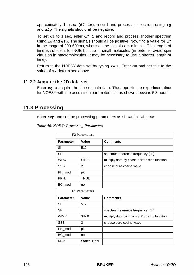
106 BRUKER Avance 1D/2D
approximately 1 msec (d7 1m), record and process a spectrum using zgand efp. The signals should all be negative.
To set d7 to 1 sec, enter d7 1 and record and process another spectrumusing zg and efp. The signals should all be positive. Now find a value for d7in the range of 300-600ms, where all the signals are minimal. This length oftime is sufficient for NOE buildup in small molecules (in order to avoid spindiffusion in macromolecules, it may be necessary to use a shorter length oftime).
Return to the NOESY data set by typing re 1. Enter d8 and set this to thevalue of d7 determined above.
11.2.2 Acquire the 2D data setEnter zg to acquire the time domain data. The approximate experiment timefor NOESY with the acquisition parameters set as shown above is 5.8 hours.
11.3 Processing
Enter edp and set the processing parameters as shown in Table 46.
Table 46: NOESY Processing Parameters
F2 Parameters
Parameter Value Comments
SI 512
SF spectrum reference frequency (1H)
WDW SINE multiply data by phase-shifted sine function
SSB 2 choose pure cosine wave
PH_mod pk
PKNL TRUE
BC_mod no
F1 Parameters
Parameter Value Comments
SI 512
SF spectrum reference frequency (1H)
WDW SINE multiply data by phase-shifted sine function
SSB 2 choose pure cosine wave
PH_mod pk
BC_mod no
MC2 States-TPPI

Avance 1D/2D BRUKER 107
Enter xfb to multiply the time domain data by the window functions and toperform the 2D Fourier transformation.
The threshold level can be adjusted by placing the cursor on the button,holding down the middle mouse button, and moving the mouse back andforth. The optimum may be saved by typing defplot and answering thequestions which appear.
11.4 Phase Correction and Plotting
For the phase correction procedure and the plotting procedure please followthe instructions given for the TOCSY spectrum in Sections 9.4 and 9.5,respectively. Note that for the NOESY spectrum recorded here, the first serialfile should be chosen for the F2 phase correction: type rser 1 instead ofrser 2, as for the TOCSY and ROESY spectra.
Figure 32: NOESY Spectrum of 50 mM Cyclosporin in C6D6

108 BRUKER Avance 1D/2D

Avance 1D/2D BRUKER 109
12 XHCORR
12.1 Introduction
Heteronuclear (X, H) shift CORRelation spectroscopy is a 2D technique thatcan be used to determine which 1H of a molecule are bonded to which 13Cnuclei (or other X nuclei). Like DEPT, XHCORR makes use of the large one-bond heteronuclear J-coupling (JXH) for polarization transfer, and thus only13C bonded directly to 1H's are detected. For 13C and directly attached 1H, JXH= 100 to 200 Hz, while for more distant 1H, JXH = 5 to 20 Hz.
The final 2D XHCORR spectrum has a projection onto the F2 axis which isthe usual 1H-decoupled 13C spectrum with all quaternary carbons missing,and a projection onto the F1 axis which is the normal 1H spectrum withreduced signal to noise since only 1H directly attached to 13C contribute to thesignal. The XHCORR experiment is not phase-sensitive, and so the final 2Dspectrum must be displayed in magnitude mode.
Reference: A. Bax and G. A. Morris, J. Magn. Reson., 42, 501 (1981).
The sample used to demonstrate XHCORR in this chapter is 1 gCholesterylacetate in CDCl3, which was used to demonstrate DEPT.
The XHCORR pulse sequence is shown in Figure 33. The short delaybetween the final 13C pulse and the start of acquisition is a refocusing periodso that the 13C lines do not have opposite phase and thus do not cancel oneanother when 1H-decoupling is applied. The optimal refocusing time (∆2)depends on whether the 13C belongs to a CH, CH2 or CH3 group. Generally acompromise value of ∆2=1/(3JXH) is chosen. 13C couplings during t1 areremoved by adding a 13C π pulse in the middle of t1, so that there isrefocusing by the end of t1. To enable maximum polarization transfer, a fixeddelay ∆1=1/(2JXH) is added after t1. This delay allows anti-phasemagnetization to be re-established.
In this pulse sequence, the delay time d2 determines the length of the delayfor the creation of anti-phase magnetization (∆1=1/(2JXH)), and the time d3determines the length of the refocusing delay (∆2=1/(αJXH)), were α is usuallychosen to be 3.

110 BRUKER Avance 1D/2D
Figure 33: XHCORR Pulse Sequence
¦ d1 ¦ d0 d0 d2 d3 acq
13C trd
π π/2
1H
π/2 π/2
t1/2
p3 p3
p2 p1
1/(αJXH) cpd t1/2 1/(2JXH)∆1 = ∆2 =
12.2 Acquisition
Insert the sample in the magnet. Lock the spectrometer. Readjust the Z andZ2 shims until the lock level is optimized. Tune and match the probehead for13C observation and 1H decoupling.
It is recommended to run 2D experiments without sample spinning.
12.2.1 Proton Reference SpectrumRecord a 1H reference spectrum to obtain the correct 1H carrier frequency(o1p) and spectral width (sw) values: Enter re proton 1 1 to call up thedata set proton/1/1; enter edc and change the following parameters
NAME xhcorrEXPNO 1PROCNO 1
Click to create the data set xhcorr/1/1.
Enter rga to perform an automatic receiver gain adjustment. Acquire andprocess a standard 1H spectrum. Calibrate the spectrum, and optimize swand o1p so that the 1H signals cover almost the entire spectral width. Acquirean optimized spectrum.
12.2.2 Carbon Reference SpectrumA 1H-decoupled 13C reference spectrum to determine the correct carrierfrequency (o1p) and spectral width (sw) values for 13C: Since XHCORRdetects only 13C directly bonded to 1H, a DEPT-45 spectrum is typically used

Avance 1D/2D BRUKER 111
as a 13C reference spectrum. Enter re dept 1 1 to call up the data setdept/1/1; enter edc and change the following parameters
NAME xhcorrEXPNO 2PROCNO 1
Click to create the data set xhcorr/2/1.
Enter rga to perform an automatic receiver gain adjustment. Acquire andprocess a 13C spectrum. Calibrate the spectrum, and optimize sw and o1p sothat the 13C signals cover almost the entire spectral width. Acquire anoptimized spectrum.
12.2.3 Acquire the 2D Data SetType xau iexpno (increment experiment number) to create the data setxhcorr/3/1.
Enter eda and set PARMODE to 2D. Click on and ok the message “Delete ‘meta.ext' files?”. The window now switches to a 2D display and themessage “NEW 2D DATA SET” appears.
Enter eda and set the acquisition parameters as shown in Table 47.
Table 47: XHCORR Acquisition Parameters
Parameter Value Comments
PULPROG hxco
hxcoqf [use this parameter for XWinNMR 3.0]
TD 1k
NS 8 the number of scans must be 4 * ns
DS 16 number of dummy scans.
PL1 high power level on F1 channel (13C) asdetermined in Section 6.1.4
PL2 high power level on F2 channel (1H) asdetermined in Section 4.2.4
PL12 low power level on F2 channel (1H) for CPDas determined in Section 6.2.6
P1 13C 90o pulse as determined in Section 6.1.4
P2 13C 180o pulse, calculated from P1
P3 1H 90° pulse as determined in Section 4.2.4
PCPD2 1H 90° pulse for cpd sequence as determinedin Section 6.2.6
D1 2 relaxation delay; should be 1–5 * T1(13C)
CNST2 145 heteronuclear scalar J(13C,1H) coupling
145 Hz is a good intermediate value
D2 3.45 msec 1/[2J(13C,1H)],

112 BRUKER Avance 1D/2D
calculated automatically from cnst2 above
CNST11 3 used to calculate d3; 3 for all multiplicities
D3 2.30 msec calculated automatically from cnst11 above
CPDPRG2 waltz16 cpd sequence for the 1H decoupling
F1 Parameters
Parameter Value Comments
TD 256 number of experiments.
FnMODE QF [use this parameter for XWinNMR 3.0]
ND0 2 two d0 periods per cycle
SW sw of the optimized 1H spectrum (xhcorr/1/1)
IN0 t1 increment, calculated from SW above
NUC1 selects 1H frequency for F1
Since this data set was created from the DEPT-45 reference spectrum, thereceiver gain is already set correctly.
Enter zg to acquire the spectrum; the approximate experiment time forXHCORR with the acquisition parameters set as shown above is 2.5 hours.
12.3 Processing
Enter edp and set the processing parameters as shown in Table 48.
Table 48: XHCORR Processing Parameters
F2 Parameters
Parameter Value Comments
SI 1k
SF spectrum reference frequency (13C)
WDW EM
LB 3 a value of 2-5 Hz is appropriate
PH_mod no this is a magnitude spectrum.
PKNL TRUE necessary when using the digital filter
BC_mod quad

Avance 1D/2D BRUKER 113
F1 Parameters
Parameter Value Comments
SI 512
SF spectrum reference frequency (1H)
WDW QSINE multiply data by squared sine function
SSB 1 choose pure sine bell
PH_mod mc this is a magnitude spectrum.
BC_mod no
MC2 QF
Enter xfb to perform the 2D Fourier transformation.
The threshold level can be adjusted by placing the cursor on the button,holding down the left mouse button, and moving the mouse up and down.The button is used to set the number of levels. The user canchoose to display positive peaks only, negative peaks only, or both positiveand negative peaks by clicking on with the left mouse button. Sincethis is a magnitude spectrum, only positive peaks need to be displayed.
Since this is a magnitude spectrum, no phase adjustment can be made.
When the spectrum appears as desired on the screen, click andanswer the following questions.
Change levels? yPlease enter number of positive levels? 6Display contours? n
12.4 Plotting the Spectrum
Read in the plot parameter file standard2D by entering rpar standard2Dplot to set most of the plotting parameters to values which are appropriatefor this 2D spectrum.
Enter edg to edit the plotting parameters. Click the ed next to the parameterEDPROJ1 to enter the F1-projection parameters submenu. Edit theparameters from PF1DU to PF1PROC as follows:
PF1DU uPF1USER (name of user for file xhcorr/1/1)PF1NAME xhcorrPF1EXP 1PF1PROC 1
Click to save these changes and return to the edg menu.

114 BRUKER Avance 1D/2D
Click the ed next to the parameter EDPROJ2 to enter the F2-projectionparameters submenu. Edit the parameters from PF2DU to PF2PROC asfollows:
PF2DU uPF2USER (name of user for file dept/4/1)PF2NAME xhcorrPF2EXP 2PF2PROC 1
Click twice to save these changes and return to main menu.
Create a title for the spectrum (setti) and plot the spectrum (plot). AnXHCORR spectrum of 1 g Cholesterylacetate in CDCl3 is shown in Figure 34.
Figure 34: XHCORR Spectrum of 1g Cholesterylacetate in CDCl3
120 100 80 60 40 20 ppm
5.0
4.0
3.0
2.0
1.0
ppm

Avance 1D/2D BRUKER 115
13 COLOC
13.1 Introduction
COLOC (COrrelation spectroscopy via LOng-range Coupling) is a 2Dheteronuclear correlation technique very similar to the XHCORR experimentdescribed in the previous Section 12. However, unlike XHCORR, COLOCmakes use also of small long-range heteronuclear J-couplings (nJXH, n > 1)for the polarization transfer, and detects all 13C, even those which are notdirectly bonded to 1H.
Because of the close similarity to the XHCORR, the COLOC experiment isonly described in brief here.
Reference: H. Kessler, C. Griesinger, J. Zarbock, and H. R. Loosli, J. Magn.Reson., 57, 331 (1984).
The sample used to demonstrate COLOC in this chapter is 1 gCholesterylacetate in CDCl3 as already used for the DEPT and XHCORRexperiments.
The COLOC pulse sequence is shown in Figure 35. The evolution time t1 isincorporated in the polarization transfer period ∆1=1/(2 nJXH): Since the long-range heteronuclear coupling constants are small (e.g. nJCH=5 to 20 Hz), thetime period ∆1 is rather long and serious sensitivity losses due to transverserelaxation are inevitable.
Figure 35: COLOC Pulse Sequence
¦ d1 ¦ d0 d0 d2 d18 acq
13C trd
π π/2
1H
π/2 π π/2
t1/2
p3 p4 p3
p2 p1
1/(αJXH) cpd t1/2
1/(n2JXH)∆1 =
∆2 =

116 BRUKER Avance 1D/2D
13.2 Acquisition and Processing
Start out from the xhcorr/3/1 data set (re xhcorr 3 1) and create the dataset coloc/1/1 (type edc and change the name to coloc and the experimentnumber to 1). The acquisition parameters are shown in Table 49.
In this pulse sequence, the delay time d6 determines the length of the delayfor the creation of anti-phase magnetization (∆1 = 1/(2 nJCH)), and the timed18 determines the length of the refocusing (∆1 = 1/(a nJCH)), where a isgenerally chosen to be 3. To ensure that the pulses occur during ∆1, the usermust make sure that d6 = d0 + (td(F1) * in0) + (p2 or p4); in other words,that d6 is at least as long as the maximum evolution time (t1) plus the lengthof the longest pulse (p2 or p4).
Table 49: COLOC Acquisition Parameters
Parameter Value Comments
PULPROG coloc
colocqf [use this parameter for XWinNMR 3.0]
TD 1k
NS 8 the number of scans must be 4 * ns
DS 16 number of dummy scans.
PL1 high power level on F1 channel (13C) asdetermined in Section 6.1.4
PL2 high power level on F2 channel (1H) asdetermined in Section 4.2.4
PL12 low power level on F2 channel (1H) for CPDas determined in Section 6.2.6
P1 13C 90o pulse as determined in Section 6.1.4
P2 13C 180o pulse, calculated from P1
P3 1H 90° pulse as determined in Section 4.2.4
P4 1H 180° pulse, calculated from P3
PCPD2 1H 90° pulse for cpd sequence as determinedin Section 6.2.6
D1 2 relaxation delay; should be 1–5 * T1(13C)
D6 50m Delay for evolution of heteronuclear scalarlong-range J(13C,1H) couplings
D18 33.3m Delay for evolution of heteronuclear scalarlong-range J(13C,1H) couplings
CPDPRG2 waltz16 cpd sequence for the 1H decoupling

Avance 1D/2D BRUKER 117
F1 Parameters
Parameter Value Comments
TD 256 number of experiments.
FnMODE QF [use this parameter for XWinNMR 3.0]
ND0 2 two d0 periods per cycle
SW sw of the optimized 1H spectrum (xhcorr/1/1)
IN0 t1 increment, calculated from SW above
NUC1 selects 1H frequency for F1
The 1H- and the 13C-reference spectra have already been recorded for theXHCORR experiment. Follow the instructions given there for the acquisitionand the processing of the 2D COLOC experiment.
A COLOC spectrum of 1g Cholesterylacetate in CDCl3 is shown inFigure 36.

118 BRUKER Avance 1D/2D
Figure 36: COLOC Spectrum of 1g Cholesterylacetate in CDCl3
160 140 120 100 80 60 40 20 ppm
5.0
4.0
3.0
2.0
1.0
ppm

Avance 1D/2D BRUKER 119
14 HMQC
14.1 Introduction
HMQC (Heteronuclear Multiple Quantum Correlation) spectroscopy is aninverse chemical shift correlation experiment that yields exactly the sameinformation as the XHCORR. The advantage of HMQC is that the nucleuswith the highest γ (1H) is detected, and so it is possible to obtain the highestsensitivity. The challenge of an inverse chemical shift correlation experiment,however, is that the large signals from 1H not coupled directly to a 13Cnucleus must be suppressed in a difference experiment. This poses adynamic range problem: the signal of interest is that of 1H coupled directly to13C nuclei; however, the signal detected is dominated by the contribution of1H bonded directly to 12C nuclei. HMQC minimizes this dynamic rangeproblem while optimizing the sensitivity of the experiment. The resonancefrequency of low γ spins can be detected with enhanced sensitivity by thecreation and 1H detection of 1H-13C (or other X nucleus) multiple-quantumcoherence.
References: A. Bax, R. H. Griffey, and B. L. Hawkins, J. Magn. Reson., 55,301 (1983); A. Bax and S. Subramanian, J. Magn. Reson., 67, 565 (1986).
The sample used to demonstrate HMQC in this chapter is 50 mMCyclosporin in C6D6. This is the same sample that was used to demonstrateCOSY, NOESY, ROESY, and TOCSY.
The HMQC pulse sequence is shown in Figure 37, which should be used onsamples consisting of proteins and other macromolecules. The first 1H pulsecreates transverse magnetization, some of which evolves into anti-phasemagnetization at the end of the first 1/(2JXH) delay. This anti-phasemagnetization is converted into multiple-quantum coherence by the (π/2)Xpulse and evolves chemical shift during t1. In analogy with XHCORR a delay1/ (2JXH) is inserted between the final 90° pulse after t1 and the start of theacquisition so that 13C decoupling can be used during acquisition. Withoutthis delay, the 1H magnetization components would be anti-phase at the startof the acquisition and so 13C decoupling would result in mutual cancellationof the 1H signals.
Note that since it is the longitudinal 1H magnetization present before the first (π/2)H pulse that is converted into heteronuclear multiple-quantum coherence,it is the 1H T1 which determines the appropriate recycle delay. Thus, it ispossible to use a shorter recycle delay for HMQC than for XHCORR.
For small molecules, it is useful to use a BIRD preparation period inconjunction with the HMQC experiment (Figure 38). The basic idea of thispreparation period is to saturate all 1H not directly attached to a 13C nucleus.

120 BRUKER Avance 1D/2D
HMQC is a phase-sensitive experiment, and after a 2D Fourier transform withrespect to t1 and t2, the 2D spectrum can be phased so that all peaks arepurely absorptive.
Figure 37: HMQC Pulse Sequence
¦ d1 ¦ d2 d2
1H trd
π/2 π
13C
π/2 π/2
1/(2JXH) t1/2 t1/2 1/(2JXH) cpd
p3 p3
p1 p2 acq
Figure 38: HMQC with BIRD Pulse Sequence
¦ d1 ¦ d2 d2 d7 d2 d0 d0 d2
1H trd
13C
π/2 π π/2 π/2 π
π π/2 π/2
1/(2JXH) t1/2 t1/2 1/(2JXH) cpd
p4 p3 p3
p1 p2 p1 p1 p2 acq
τT
14.2 Acquisition
Insert the sample in the magnet. Lock the spectrometer. Readjust the Z andZ2 shims until the lock level is optimized. Tune and match the probehead for1H observation and 13C decoupling.
It is recommended to run 2D experiments without sample spinning
As for the XHCORR experiment, both 1H and 13C reference spectra of thissample must be recorded; see Sections 12.2.1 and 12.2.2 for the

Avance 1D/2D BRUKER 121
corresponding instructions. Use wrpa to store the reference spectra as datasets hmqc/1/1 (for the 1H spectrum) and hmqc/2/1 (for the 13C spectrum).
Enter re hmqc 1 1 to return to the optimized 1H spectrum. Create the dataset hmqc/3/1 by using edc.
Enter edsp and set NUC2 to 13C.
Set o2p to the value found for the optimized 13C spectrum in hmqc/2/1.
Enter eda and set PARMODE = 2D. Click on and ok the message“Delete ‘meta.ext' files?”. The window now switches to a 2D display and themessage “NEW 2D DATA SET” appears.
Enter eda and set the acquisition parameters as shown in Table 50.
Table 50: HMQC with BIRD Acquisition Parameters
F2 Parameters
Parameter Value Comments
PULPROG invbst
invbph
HMQC with BIRDfor HMQC without BIRD choose inv4tp
[use this parameter for XWinNMR 3.0, forHMQC without BIRD in 3.0 choose inv4ph]
TD 1k
NS 8 the number of scans should be 4 *
DS 16 number of dummy scans.
PL1 high power level on F1 channel (1H) asdetermined in Section 4.2.4
PL2 high power level on F2 channel (13C) asdetermined in Section 6.1.4
PL12 low power level on F2 channel (13C) for CPDas determined in Section 6.3.7
P1 1H 90o pulse as determined in Section 4.2.4
P2 1H 180o pulse, calculated from P1
P3 13C 90° pulse as determined in Section 6.1.4
P4 13C 180o pulse, calculated from P3
PCPD2 13C 90° pulse for cpd sequence as determinedin Section 6.3.7
D1 1.5 relaxation delay; should be 1–5 * T1(1H)
CNST2 145 heteronuclear scalar J(13C,1H) coupling
145 Hz is a good intermediate value
D2 3.45 msec 1/[2J(13C,1H)],
calculated automatically from cnst2 above
CPDPRG2 garp cpd sequence for the 13C decoupling
D7 100 msec delay for inversion recovery (optimize)

122 BRUKER Avance 1D/2D
F1 Parameters
Parameter Value Comments
TD 256 number of experiments.
FnMODE States-TPPI [use this parameter for XWinNMR 3.0]
ND0 2 there are two d0 periods per cycle
IN0 t1 increment.
SW 190 sw of the 13C spectrum ,typically 190 ppm
NUC1 select 13C frequency for F1
14.2.1 Optimize d7 (only for HMQC with BIRD)Set the acquisition parameters as shown above and choose a starting valueof 400 msec for d7. Enter acqu to enter the acquisition window. Enter gs tostart the go setup routine. Click the left mouse button to fix the acquisition-gswindow somewhere on the screen, and then click on the box in the upperright hand corner of the window to iconize it. While monitoring the intensity ofthe time domain data, adjust the value of d7 (simply enter d7 and then a newvalue at the prompt). The optimum value of d7 corresponds to the minimumsignal intensity. Once the optimum value of d7 is found and stored, enter rgato optimize the receiver gain for this minimum signal.
14.2.2 Acquire the 2D data setEnter zg to start the HMQC experiment. With the acquisition parametersshown above, the approximate experiment time is 1.2 hours.
14.3 Processing
Enter edp and set the processing parameters as shown in Table 51.
Table 51: HMQC with BIRD Processing Parameters
F2 Parameters
Parameter Value Comments
SI 1k
SF spectrum reference frequency (1H)
WDW QSINE sine-squared window function
SSB 2 pure cosine-squared wave
PH_mod pk apply 0- and 1st-order phase correctiondetermined by phase correcting the first row
PKNL TRUE necessary when using the digital filter.
BC_mod no

Avance 1D/2D BRUKER 123
F1 Parameters
Parameter Value Comments
SI 512
SF spectrum reference frequency (13C)
WDW QSINE sine-squared window function
SSB 2 pure cosine-squared wave
PH_mod pk apply 0- and 1st-order phase correctiondetermined by automation program calcphinv
BC_mod no
MC2 States-TPPI
Enter xfb to multiply the time domain data by the window functions and toperform the 2D Fourier transformation.
The threshold level can be adjusted by placing the cursor on the button,holding down the middle mouse button, and moving the mouse back andforth. Both positive and negative peaks can be displayed by clicking on the
button. The optimum may be saved by typing defplot and answeringthe questions which appear.
14.4 Phase Correction
Enter rser 1 to transfer the first row to the 1D data set ~TEMP/1/1. Entersinm to apply the sine-bell windowing function, and enter ft to Fouriertransform the data. Manually phase correct the spectrum. Click andselect Save as 2D & return to save the corrections phc0 and phc1 to thecorresponding F2 parameters in the 2D data file hmqc/3/1. Click with theleft mouse button to return to the 2D data set hmqc/3/1.
It is convenient to use an automation program to determine the F1 phasecorrection. From the data set hmqc/3/1, simply enter xau calcphinv. Notethat this automation program is designed specifically for HMQC-typeexperiments.
Now enter xfb to Fourier transform the HMQC spectrum again using theappropriate phase correction to F1 and F2. The spectrum should be phasedcorrectly and all peaks should be positive. Further adjustments can be madein the 2D phase subroutine, as described in previous chapters.
14.5 Plotting
Follow the instructions given for the previous experiments, i.e., XHCORR. AnHMQC spectrum of 50 mM Cyclosporin in C6D6 is shown in Figure 39.

124 BRUKER Avance 1D/2D
Figure 39: HMQC Spectrum of 50 mM Cyclosporin in C6D6

Avance 1D/2D BRUKER 125
15 HMBC
15.1 Introduction
HMBC (Heteronuclear Multiple Bond Correlation) spectroscopy is a modifiedversion of HMQC suitable for determining long-range 1H-13C connectivities.Since it is a long-range chemical shift correlation experiment, HMBC providesbasically the same information as COLOC but it has a higher sensitivity,since it is an inverse experiment.
Reference: A. Bax and M. F. Summers, J. Am. Chem. Soc., 108, 2093(1986).
The sample used to demonstrate HMBC in this chapter is 50 mM cyclosporinin C6D6 as was used to demonstrate HMQC.
The HMBC pulse sequence is shown in Figure 40. The first 13C 90° pulse,which is applied 1/(2 1JXH) after the first 1H 90° pulse, serves as a low-pass J-filter to suppress one-bond correlations in the 2D spectrum by creating 1H-13C heteronuclear multiple quantum coherence. This unwanted coherence isremoved by phase cycling the first 13C 90° pulse with respect to the receiver.After the delay ∆2 of about 60msec, the second 13C 90° pulse creates thedesired heteronuclear multiple-quantum coherence for long-range 1H-13C J-couplings. Phase cycling of the second 13C 90°pulse removes signals from1H without long-range coupling to 13C. The final 13C 90°pulse after the t1evolution period is followed immediately by the detection period t2. The signaldetected during t2 is phase modulated by the homonuclear 1H J-couplings.The 2D spectrum is generated by a Fourier transform with respect to t1 andt2. If more than one long-range 1H-13C connectivity is detected for oneparticular proton, the relative intensities of the corresponding resonances aredirectly related to the magnitude of the coupling constant.
Because of phase modulation the spectrum has peaks with a combinedabsorptive and dispersive lineshape. It is not possible to phase correct thespectrum so that the peaks are purely absorptive, and so the spectrum mustbe presented in magnitude mode.
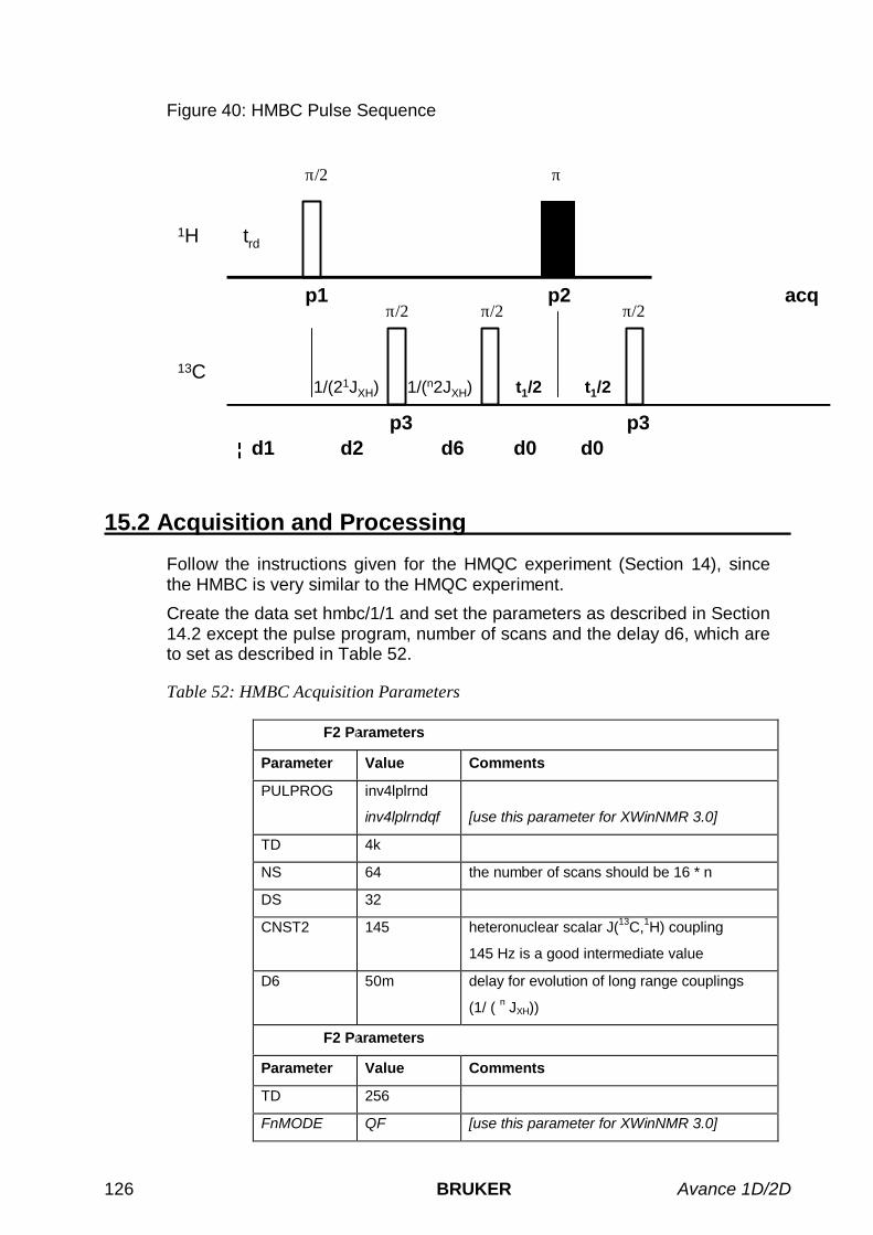
126 BRUKER Avance 1D/2D
Figure 40: HMBC Pulse Sequence
¦ d1 d2 d6 d0 d0
π/2 π
π/2 π/2 π/2
1/(n2JXH) t1/2 t1/2
p3 p3
p1 p2 acq
1H trd
13C1/(21JXH)
15.2 Acquisition and Processing
Follow the instructions given for the HMQC experiment (Section 14), sincethe HMBC is very similar to the HMQC experiment.
Create the data set hmbc/1/1 and set the parameters as described in Section14.2 except the pulse program, number of scans and the delay d6, which areto set as described in Table 52.
Table 52: HMBC Acquisition Parameters
F2 Parameters
Parameter Value Comments
PULPROG inv4lplrnd
inv4lplrndqf [use this parameter for XWinNMR 3.0]
TD 4k
NS 64 the number of scans should be 16 * n
DS 32
CNST2 145 heteronuclear scalar J(13C,1H) coupling
145 Hz is a good intermediate value
D6 50m delay for evolution of long range couplings
(1/ ( n JXH))
F2 Parameters
Parameter Value Comments
TD 256
FnMODE QF [use this parameter for XWinNMR 3.0]

Avance 1D/2D BRUKER 127
Enter zg to start the HMBC experiment. With the acquisition parametersshown above, the approximate experiment time is 13.5 hours.
Enter edp and set the processing parameters as shown in
Table 53.
Table 53: HMBC Processing Parameters
F2 Parameters
Parameter Value Comments
SI 2k
SF spectrum reference frequency (1H)
WDW QSINE sine-squared window function
SSB 0 pure sine-squared wave
PH_mod no
PKNL TRUE necessary when using the digital filter.
BC_mod quad
F1 Parameters
Parameter Value Comments
SI 512
SF spectrum reference frequency (13C)
WDW SINE sine window function
SSB 0 pure cosine wave
PH_mod mc
MC2 QF
Enter xfb to multiply the time domain data by the window functions and toperform the 2D Fourier transformation.
Adjust the display as described for the HMQC spectrum.
An HMBC spectrum of 50 mM Cyclosporin in C6D6 is shown in Figure 41.

128 BRUKER Avance 1D/2D
Figure 41: HMBC spectrum of 50 mM Cyclosporin in C6D6

Avance 1D/2D BRUKER 129
16 Proton-Carbon Inverse ShiftCorrelation- Experiments usingPulsed Field Gradients
16.1 Introduction
The three most common inverse chemical shift correlation experiments areHSQC, HMQC and HMBC, which are used to determine which 1H of amolecule are bonded to which 13C nuclei (or other X nuclei). The advantageof inverse experiments over X detection experiments is that with inverseexperiments the nucleus with the highest γ (usually 1H) is detected yieldingthe highest sensitivity. The challenge of an inverse chemical shift correlationexperiment, however, is that the large signals from 1H not coupled directly toa 13C nucleus must be suppressed in a difference experiment, which poses adynamic range problem. Common techniques for the suppression of 1Hbound to 12C are the BIRD-sequence in HMQC experiments and a trim pulseof 1-2ms during the first INEPT in HSQC experiments. However, thesuppression is still imperfect and usually additional phase cycling is required.The introduction of pulsed field gradients in high-resolution NMR greatlyimproved the problem of suppressing signals from 1H bonded to 12C: Thesuppression is almost perfect without additional phase cycling.
In general, NMR experiments using PFGs are called GRASP experiments:GRASP-HSQC, GRASP-HMQC, GRASP-HMBC etc.
Details on the GRASP technique are covered by the GRASP course and willnot be discussed here.
16.2 GRASP-HMQC
See Section 14 for information about the HMQC experiment.
The GRASP-HMQC pulse sequence is shown in Figure 42. The PFGs in theexperiment are used for coherence selection and the quadrature detection inthe ω1 dimension. The two gradients applied during t1 (gradients G1 and G2)dephase all 1H magnetization, while the third gradient G3 rephases themagnetization of interest.
The gradient ratio G1+G2:G3 for a GRASP-HMQC is 2:1 for 13C and 5:1 for15N.
This version of the GRASP-HMQC experiment is not phase sensitive.

130 BRUKER Avance 1D/2D
Figure 42: GRASP-HMQC Pulse Sequence
¦ d1 d2 d0 d0
π/2 π
π/2 π/2
t1/2 t1/2
p3 p3
p1 p2 acq
1H trd
13C1/(21JXH)
G1 G2 G3
Gradient
Note that all correlation peaks of any HMQC experiment are splitted alongthe ω1 dimension due to evolution of the homonuclear 1H-1H coupling, whichcannot be refocussed by the 180o 1H pulse applied during t1. Therefore, theresolution of the HMQC experiment along the ω1 dimension is limited. For abetter resolution in the ω1 dimension the HSQC experiments must be done.
References: A. Bax, R. H. Griffey, and B. L. Hawkins, J. Magn. Reson., 55,301 (1983); A. Bax and S. Subramanian, J. Magn. Reson., 67, 565 (1986).
16.3 GRASP-HMBC
See Section 15 for information about the HMBC experiment.
The GRASP-HMBC pulse sequence is shown in Figure 43. Identical gradientratios are used for the GRASP-HMBC as for the GRASP-HMQC (see Section16.2).

Avance 1D/2D BRUKER 131
Figure 43: GRASP-HMBC pulse sequence
¦ d1 d2 d6 d0 d0
π/2 π
π/2 π/2 π/2
1/(n2JXH) t1/2 t1/2
p3 p3 p3
p1 p2 acq
1H trd
13C1/(21JXH)
G1 G2 G3
Gradient
16.4 GRASP-HSQC
HSQC (Heteronuclear Single Quantum Correlation) yields the samespectrum as HMQC but is based on single-quantum NMR. In the HSQCsequence, the pulse scheme prior the t1 evolution period represents a socalled INEPT sequence and creates transverse single-quantummagnetization on the X-nucleus, e.g., 13C or 15N, which evolves X chemicalshift during t1. The G1 gradient dephases all the transverse magnetization.This gradient is located in a spin echo in order to refocus chemical shiftevolution during the gradient. Then, a second INEPT segment transfers themagnetization to 1H, where it is detected after it has been rephased by asecond gradient G2.
The field gradients in this version of a GRASP-HSQC experiment are solelyused for the coherence selection. The gradient ratio G1:G2 for a GRASP-HSQC is 4:1 for 13C and 10:1 for 15N.
This version of the GRASP-HMQC experiment is phase sensitive.
Compared to the HMQC experiment no line broadening along the ω1dimension appears as only 13C single-quantum magnetization is presentduring the t1 evolution period.
References: A. Bax, R. H. Griffey, and B. L. Hawkins, J. Magn. Reson., 55,301 (1983); A. Bax and S. Subramanian, J. Magn. Reson., 67, 565 (1986).
Pulse sequence for GRASP-HSQC is shown in Figure 44.

132 BRUKER Avance 1D/2D
Figure 44: GRASP-HSQC Pulse Sequence
¦ d1 d4 d4 d0 d0 DELTA d24 d24 d4 d4 DELTA1
π/2 π trim
p4 p3 p4 p3 p4 p3 p4
p1 p2 p28 p1 p2 p1 p2 p1 p2 p1 p2 acq
1 H trd
13C
+/-G1 G2
Gradient
π π / 2
t1/2 t1/2
1/(41JXH) 1/(81JXH) or 1/(41JXH)
16.5 Acquisition and Processing
The GRASP experiments are best started from a corresponding data setwithout gradients, e.g. for the GRASP-HMQC and GRASP-HSQC from theHMQC data set (re hmqc 3 1) (Section 14) or HMBC (Section 15).
Table 54: 1H,13C HMQC, HMBC and HSQC Acquisition Parameters
F2 Parameters
Parameter Value Comments
PULPROG inv4gp
inv4gplplrnd
invietgpsi
For GRASP-HMQC
For GRASP-HMBC
For GRASP-HSQC.
inv4gpqf
inv4gplplrndqf
invietgpsi
[For GRASP-HMQC in XWinNMR 3.0]
[For GRASP-HMBC in XWinNMR 3.0]
[For GRASP-HSQC in XWinNMR 3.0]
TD 2k
NS 2
8
For GRASP-HMQC GRASP-HSQC
For GRASP-HMBC
DS 16 number of dummy scans, has to be ns*2*n

Avance 1D/2D BRUKER 133
P28 0.5u Trim pulse in HSQC
Do not set it to a longer value
D4 1.72msec For HSQC only: 1/[2 1J(13C,1H)],
calculated automatically from cnst2 above
D24 0.86msec For HSQC only: delay for refocussing JCH.
For all multiplicities set the value to:
1/[8 1J(13C,1H)]
Only for CH-groups set the value to:
1/[4 1J(13C,1H)] = D4
F1 Parameters
Parameter Value Comments
TD 256 number of experiments.
FnMODE QF
echo-antiecho
QF
[For GRASP-HMQC in XWinNMR 3.0]
[For GRASP-HSQC in XWinNMR 3.0]
[For GRASP-HMBC in XWinNMR 3.0]
ND0 2
IN0 t1 increment.
SW 190ppm
260ppm
For HSQC and HMQC
For HMBC
NUC1 select 13C frequency for F1
Gradient Parameters for the gp-syntax
Parameter Value Comments
P16 1.5ms Length of gradient pulses
D16 150u Gradient recovery delay
gpz1 50
80
For HMQC and HMBC
For HSQC
gpz2 30
20.1
For HMQC and HMBC
For HSQC
gpz3 40.1 For HMQC and HMBC
gpnam1 SINE.100 gradient shape
gpnam2 SINE.100 gradient shape
gpnam3 SINE.100 gradient shape
With the acquisition parameters shown above, the approximate experimenttimes are 0.3h for HMQC and HSQC, and 1.2 hours for HMBC.
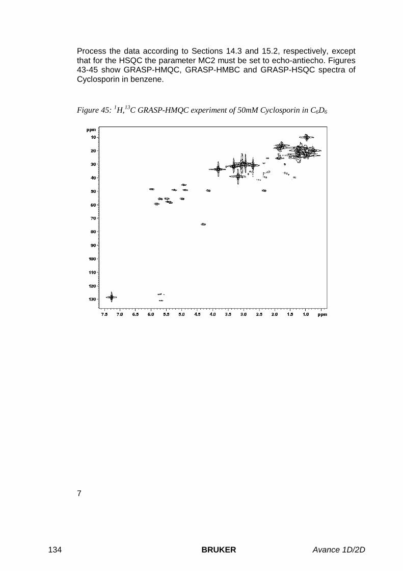
134 BRUKER Avance 1D/2D
Process the data according to Sections 14.3 and 15.2, respectively, exceptthat for the HSQC the parameter MC2 must be set to echo-antiecho. Figures43-45 show GRASP-HMQC, GRASP-HMBC and GRASP-HSQC spectra ofCyclosporin in benzene.
Figure 45: 1H,13C GRASP-HMQC experiment of 50mM Cyclosporin in C6D6
7

Avance 1D/2D BRUKER 135
Figure 46: 1H,13C GRASP-HMBC experiment of 50mM Cyclosporin in C6D6
Figure 47: 1H,13C GRASP-HSQC experiment of 50mM Cyclosporin in C6D6

136 BRUKER Avance 1D/2D

Avance 1D/2D BRUKER 137
17 1D NOE Difference
17.1 Introduction
The Nuclear Overhauser Effect (NOE) is a net change of the signal intensityfrom one spin due to the relaxation of a saturated spin that is dipole-dipolecoupled to the first spin. NOE's develop due to through-space rather thanthrough-bond interactions, and thus contain information on the distancesbetween spins.
The rate or efficiency of the NOE buildup depends on the rate or efficiency ofthe dipole-dipole relaxation, which itself depends on the strength andfrequency of the fluctuating fields. These fluctuating fields depend on thedistance between the nuclei involved, the tumbling rate of the molecule, andthe characteristics of the nuclei themselves. The presence of paramagneticmolecules (e.g., metal ions, rust, or dissolved oxygen) distorts any NOEexperiment, since they dominate T1 relaxation processes.
In an NOE difference experiment, a 1H resonance is selectively preirradiateduntil saturation is achieved. During the preirradiation period, NOE buildupoccurs at other 1H nuclei close in space. A π/2 pulse then creates observablemagnetization, which is detected during the acquisition period. Theexperiment is repeated using different preirradiation frequencies, includingone which is off-resonance. The latter is used to obtain a reference or controlspectrum. The final spectra are displayed as the difference between aspectrum recorded with on-resonance preirradiation and the referencespectrum.
Very small phase or frequency shifts between two spectra will give rise toimperfect signal subtraction. To minimize subtraction artifacts an efficientsignal averaging and maximal acceptable line broadening should be used.Other artifacts from temperature instability or magnetic field drift may beminimized by acquiring the preirradiated and the reference data in aninterleaved manner.
Reference: D. Neuhaus and M. P. Williamson, “The Nuclear OverhauserEffect in Structural and Conformational Analysis,” New York: VCHPublishers, Inc., 1989.
The sample used to demonstrate a 1D NOE difference experiment in thischapter is 100 mM Pamoic Acid in DMSO-d6.
The NOE difference pulse sequence is shown in Figure 48. The pulsesequence begins with the recycle delay time d1. This is followed by the cwirradiation period of total time l4*d20, where d20 is the irradiation time forone particular frequency. The pulse program makes use of a frequency list(fq2list) to determine the frequencies for cw irradiation. The final 90°

138 BRUKER Avance 1D/2D
pulse p1 creates the observable magnetization and is followed by theacquisition period.
Several spectra are acquired during an NOE difference experiment, and foreach spectrum a different fq2list is used. For the reference spectrum, thecw pulse is applied off-resonance and the au program noemult is used toacquire the spectra in an interleaved manner.
Figure 48: 1D NOE Difference Pulse Sequence
¦ d1 ¦ L14*d20 ¦ p1 acq
1H trd cw
π/2
17.2 Acquisition
Insert the sample in the magnet. Lock the spectrometer. Readjust the Z andZ2 shims until the lock level is optimized. Tune and match the probehead for1H observation.
For best results it is recommended to optimize the lock parameters asdescribed. NOE difference experiments should be run without samplespinning.
The parameters and spectra shown below are from a 300 MHz spectrometer.The signal enhancements for Pamoic Acid in DMSO-d6 at other fieldstrengths will be different than those shown here. If an NOE response isdifficult to obtain, it may be necessary to change the sample temperature orsolvent. In particular for this sample at 400 MHz, it is recommended to use atemperature of 40°C.
17.2.1 Create a new file directoryEnter re proton 1 1 to call up the data set proton/1/1. Enter edc and createthe data set noediff/1/1.
Enter edasp and set both NUC1 and NUC2 to 1H. The f2 channel is used forcw irradiation during the NOE experiment.
17.2.2 Proton reference spectrumEnter rga to perform an automatic receiver gain adjustment. Acquire andprocess a standard 1H spectrum, as described in Chapter 3. Calibrate the

Avance 1D/2D BRUKER 139
spectrum and optimize sw and o1p. Keep in mind that the control spectrumshould be irradiated well off-resonance (in this case –2 ppm). Acquire andprocess an optimized spectrum.
17.2.3 Select the resonances for irradiationThe frequencies used by the f2 channel during the preirradiation periods ofthe NOE experiment must be written to the corresponding fq2list. Aseparate list must be created for each resonance to be irradiated, where agiven list may contain several frequencies if irradiation of a resonance atseveral points is needed. One of the lists must contain a frequency well off-resonance for generating the reference spectrum.
Here, we will create lists with frequencies for the resonances at 4.8 ppm and8.5 ppm, and one with the off-resonance frequency –2 ppm. The frequencylists are defined using the routine, which is found in the submenu .
Note that if it is necessary to expand the spectrum in order toaccurately define the irradiation points this must be done before entering theroutine. Display the peak at 4.8 ppm and enter the routine andanswer the questions as shown below:
Please enter type of list (f1, f2, f3): f1Please enter name of f1 list: noedif.1Write name of f1 list to acqu parameters? n
The following option appears if a f1 frequency list with the same namealready exists:
Frequency list exists, append (a), overwrite (o) or quit (q):
Answer a if you wish to add new frequencies to the existing list, o if you wishto overwrite the existing list, or q if you wish to quit the routine and keep theold list.
Once the questions have been answered, move the mouse until the cursor istied to the spectrum. Click on the peak at 4.8 ppm with the middle mousebutton. Finish the list by clicking the left mouse button. Remember that for agiven list, multiple irradiation points should all be part of the same multiplet. Aseparate frequency list should be generated for each multiplet irradiated.
Note: The “type of list (f1, f2, f3)” refers to the directory where the frequencylist is stored and not to the spectrometer channel for which the list will beused). In any acquisition parameter set it is possible to define eight separatefrequency lists (fq1list, fq2list, etc.). The pulse program noemul usesonly one frequency list: fq2list. Therefore, set the parameter fq2list tothe appropriate list name “noedif.1” within the eda menu, The automationprogram noemult redefines fq2list each time noemul is to be run with adifferent frequency list.
Repeat this procedure for the peak at 8.5 ppm and for the off-resonancefrequency of –2 ppm. Write the lists to the files noedif.2 and noedif.3,respectively. Note that the automation program noemult requires that allfrequency lists have the same base name and increasing extension numbers.
Click on to leave the utilities submenu and return to the main menu.

140 BRUKER Avance 1D/2D
17.2.4 Set up the acquisition parametersEnter edc and change EXPNO to 2 to create the data set noedif/2/1.
Enter eda and set the acquisition parameters as shown in Table 55. Verifythat NUC2 has been set to 1H in edasp.
Table 55: 1D NOE Difference Acquisition Parameters
Parameter Value Comments
PULPROG noemul
TD 64k
NS 8 the number of scans must be 8 * n
DS 2
PL1 high power level on F1 channel (1H) asdetermined in Section 4.2.4
PL14 70 power level for NOE buildup
P1 1H 90o pulse as determined in Section 4.2.4
D1 3.5 relaxation delay
D20 50m 50 msec irradiation time
L4 T1 / D20 loop counter to determine overall irradiationtime (T1 = L4 * D20)
FQ2LIST noedif.1 frequency list for f2 frequency of selectiveirradiation
The pulse program noemul operates such that o2 is set to the first frequencyof the fq2list and the selected multiplet is irradiated with this frequency fora time d20. Then o2 is set to the next frequency (if there is one) of thefq2list and the selected multiplet is irradiated with this frequency for atime d20. This process continues until the multiplet is irradiated for a total ofl4 times.
17.2.5 Optimize the irradiation power and durationFor the NOE difference experiment, the au program noemult will run thepulse program noemul with successive fq2lists. However, the optimization ofirradiation power and duration can be performed for a single resonance.Thus, the au program is not necessary and the pulse program noemul canbe started with the command zg.
Make sure that fq2list is set to noedif.1 (or noedif.2, i.e., make surethat the cw irradiation will be applied on resonance for one of the multiplets).Start the acquisition with zg, process the spectrum with ef (see theprocessing parameters listed below in Table 56), and manually phase correctthe spectrum.
Compare this spectrum with the reference spectrum noedif/1/1 by using thedual mode. From the current data set (noedif/2/1), enter edc2 to define the

Avance 1D/2D BRUKER 141
second data set to be shown in the dual display. Set EXPNO2 to 1 andPROCNO2 to 1 and click .
Click to enter the dual display mode. Both the spectra fromnoedif/1/1 and noedif/2/1 appear in the window. When the comparison of thespectra is finished, click to return to the main 1D processing window.
Ideally, the target resonance is completely saturated by the selectiveirradiation, while all other signals are unaffected by the irradiating field. Inpractice, the chemical shift difference between signals is often too small, sothat neighboring resonances may be saturated as well.
It is almost always preferable to use low-power (and hence selective)irradiation rather than unwanted saturation of nearby resonances. However,partial saturation of a multiplet leads to selective population transfer whichmay obscure NOE effects. To avoid this, the individual components of atarget multiplet are irradiated in an interleaved manner during thepreirradiation period before each scan.
If needed, adjust pl14 to change the power level of the cw irradiation.
Note that the total cw irradiation time (l4*d20) should be approximatelyequal to T1 of the irradiated peak, but with the au program noemult, it isnecessary to use the same total irradiation time for each peak irradiated.Thus, the irradiation time should be chosen based on the longest T1. Here atotal irradiation time of 2.5 sec is used, which is longer than the T1 of thepeak at 8.5 ppm.
17.2.6 Perform the multiple NOE experimentTo start the NOE difference experiment, type xau noemult and answer thequestions as follows:
base name of all frequency lists: noedif# of frequency lists: 3# of cycles through each list: L4# of average cycles: 8
The number of frequency lists is the number of fq2lists written above and itwill be the number of spectra acquired. The number of cycles through eachlist is the loop counter l4. The number of average cycles controls the totalnumber of scans for each frequency list. For each frequency list (and hence,for each spectrum) the total number of scans is ns, where ns should be assmall as possible (e.g., 8) and then the signal-to-noise ratio is improved byincreasing the number of average cycles (to, e.g., 10).
The au program automatically starts the pulse program noemul using theacquisition parameters defined in the current data set (noedif/2/1) and the o2frequencies defined in the first fq2list (noedif.1). Next, an experiment isperformed using the o2 frequencies defined in the second fq2list (noedif.2)and the results are written to the next data set (noedif/3/1) and so on. Note,that new data sets created by noemult have the same name as the originaldata set, but increasing EXPNO. Here, the spectrum irradiated at 4.5 ppm isnoedif/2/1, that at 8.5 ppm is noedif/3/1, and that at –2 ppm is noedif/4/1.

142 BRUKER Avance 1D/2D
The entire cycle is repeated until the experiment is finished. The number oftimes this cycle is performed is determined by the value entered for thenumber of average cycles.
17.3 Processing
Enter edp and set the processing parameters as shown in Table 56.
Table 56: 1D NOE Difference Processing Parameters
Parameter Value Comments
SI 8k
WDW EM
LB 0.3
PKNL TRUE
17.3.1 Perform the Phase CorrectionTo process the spectra acquired by noemult it is necessary to define thephase correction parameters first.
Read in the first file (re 2 1). Apply the window function and Fouriertransformation with the command ef. Manually phase correct the spectrumand store the correction (see Section 3.8).
All spectra are processed identically by entering xau multiefp and answerthe questions as follows:
Enter first expno to process: 2Enter number of expnos: 3
Here, the “first expno to process” indicates the spectrum that is alreadyFourier transformed and phase corrected. The au program multiefp readsall processing parameters (including 0th- and 1st-order phase corrections)from this data set and uses them to process the following three spectra withthe same data set name
At this point the data consists of a series of spectra with various saturatedresonances and one reference spectrum. The procedure for creating thedifference spectra is outlined below.
17.3.2 Create NOE Difference SpectraThe NOE difference spectra are created by subtracting the referencespectrum from each of the preirradiated spectra. Within the data set of eachpreirradiated spectrum, the second and third data sets are defined by usingthe edc2 command, where the second data set refers to the referencespectrum and the third data set refers to the data set where the differencespectrum is stored.

Avance 1D/2D BRUKER 143
Display the first preirradiated spectrum (re 2 1). Enter edc2 and setEXPNO2 and PROCNO2 to 4 and 1, respectively (reference spectrum). SetEXPNO3 and PROCNO3 2 and 2, respectively, so that the differencespectrum will be stored with the same experiment number and processingnumber 2. Click on to the main menu.
Enter the dual submenu by clicking on . Both the current spectrumand the reference spectrum appear on the screen. Click on andselect Save & return to subtract the reference spectrum from the currentpreirradiated spectrum. The difference spectrum appears automatically in thewindow.
Click to save the results and return to the main menu. Themessage “result will be put into: DU = u, USER = <username>, NAME =noedif, EXPNO = 2, PROCNO = 2, click OK if ok” appears. Click OK andnotice that the current data set is now noedif/2/2.
Move to the next preirradiated spectrum (re 3 1) and repeat the aboveprocedure (set EXPNO2 = 4, PROCNO2 = 1, EXPNO3 = 3 and PROCNO2 =2 to store the difference spectrum in noedif/3/2).
Two NOE difference spectra (with cw irradiation on-resonance at 8.5 ppmand 4.8 ppm) and the reference spectrum (with cw irradiation off-resonanceat –2 ppm) of 100 mM Pamoic Acid in DMSO-d6 are shown in Figure 49.
In both the difference spectra with cw irradiation at 8.5 ppm and 4.8 ppm, thelarge negative peak is the irradiated resonance and the small positive doubletis the NOE. Note that these spectra were recorded on a DPX300 at 298 K.Experiments recorded at 500 MHz and 298 K will have negative NOE peaks,while those recorded at 400 MHz and 298 K may show no NOE peaks at all.
17.3.3 Quantitate the NOETo quantitate an observed NOE, the integrated intensity of the NOE peak inthe difference spectrum is compared with the integrated intensity of the peakthat was irradiated. However, this latter intensity should be measured in thereference spectrum. Thus, it is necessary to integrate peaks in both thecontrol and the difference spectrum, and to use the same normalizationconstant for the integrals in both spectra (see Section 3.10).

144 BRUKER Avance 1D/2D
Figure 49: NOE Difference Spectra of 100 mg Pamoic Acid in DMSO
9.0 8.0 7.0 6.0 5.0 ppm
reference
8.5 ppm
4.8 ppm

Avance 1D/2D BRUKER 145
18 Homonuclear decoupling
18.1 Introduction
The technique of homonuclear decoupling (double resonance, spindecoupling, homo decoupling) was established long before routine pulsed FTspectroscopy became popular. In those days the usual NMR experimentconsisted of applying a variable field B1 to the sample for the observation ofthe absorption spectrum (so-called continuous wave method). Doubleresonance or homonuclear decoupling is the term used for experiments inwhich a field B2 in addition to B1 is applied to the sample.
On modern FT spectrometers equipped with a single coil probe-head, thisdecoupling requires a special mode in order to apply the decoupling energy(B2) during the acquisition. The so-called hd-mode is applying the energy inpulsed mode within the duty cycle of the dwell time and the preamplifier isswitched off during the decoupler pulses.
The underlying principles of homonuclear decoupling can be illustrated byconsidering e.g. the molecule ethyl benzene and coupling pattern of the ethylgroup. Irradiation of the methylene group will result in the collapse of themethyl group to a singulet and vice versa. (Figure 50).
Figure 51: Spectra of ethyl benzene without and with homo decoupling
234567 ppm

146 BRUKER Avance 1D/2D
Suitable samples to setup homo decoupling are the proton sensitivity sample0.1% ethyl benzene in CDCl3 or 100mM pamoic acid in DMSO-d6.
18.2 Acquisition
Insert the sample in the magnet. Lock the spectrometer. Readjust the Z andZ2 shims until the lock level is optimized. Tune and match the probehead for1H observation. This experiment can be run with sample rotation.
18.2.1 Create a new file directoryEnter re proton 1 1 to call up the data set proton/1/1. Enter edc and createthe data set homodec/1/1.
Enter edasp and set both NUC1 and NUC2 to 1H. The f2 channel is used forcw irradiation during the NOE experiment.
18.2.2 Proton reference sepctrumEnter rga to perform an automatic receiver gain adjustment. Acquire andprocess a standard 1H spectrum, as described in Chapter 3. Calibrate thespectrum and optimize sw and o1p. Acquire the standard spectrum using theparameters outlined in the table :
Table 57: Acquisition Parameters for 1H Reference Spectrum
Parameter Value Comments
PULPROG zg30 One pulse acquisition with 30° flip angle
NS 8 number of scans
DS 2 number of dummy scans
Process the FID with em, ft and phase correct it.
18.2.3 Selection of irradiation frequencyThe frequency used by the f2 channel for the irradiation of the multiplet canbe defined by entering the submenu and clicking on the button forselecting the o2 frequency . The cursor is now bound to the spectrumand changed his shape (vertical arrow). The mouse buttons in this mode dohave the functions
left=return
middle=define frequency
right=unused.
Move the cursor to the position of interest and press the middle mouse buttonto define SFO2/O2 frequency. Leave the utilities submenu with the returnbutton. The determined value for o2 is now stored in the current data set.

Avance 1D/2D BRUKER 147
18.2.4 Setting up the homo decoupling parameters
Enter edc and change EXPNO to 2 to create the data set homodec/2/1.
Setup the relevant parameters according to the table.
Table 58: Acquisition Parameters for homo decoupling
Parameter Value Comments
PULPROG zghd.2 Pulse program for homo decoupling
CPDPRG2 hd Decoupling sequence during relaxation
PL 24 ~ 50 Needs to be optimized for good decoupling
DIGMOD For AV instruments: digital
For D..X instruments: homodecoupling-digital
HDDUTY 20% To be only set with XWINNMR 3.0
Optimise pl24 until the multiplet of interest collapses completely to e.g. asingle line. Be careful when increasing the power, values below 40dB shouldbe avoided!
The phase correction values of a homo decoupled spectrum is different to thereference spectrum and must therefore be adjusted for each irradiated signal.

148 BRUKER Avance 1D/2D
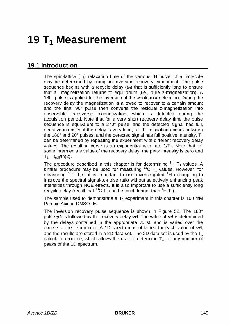
Avance 1D/2D BRUKER 149
19 T1 Measurement
19.1 Introduction
The spin-lattice (T1) relaxation time of the various 1H nuclei of a moleculemay be determined by using an inversion recovery experiment. The pulsesequence begins with a recycle delay (trd) that is sufficiently long to ensurethat all magnetization returns to equilibrium (i.e., pure z-magnetization). A180° pulse is applied for the inversion of the whole magnetization. During therecovery delay the magnetization is allowed to recover to a certain amountand the final 90° pulse then converts the residual z-magnetization intoobservable transverse magnetization, which is detected during theacquisition period. Note that for a very short recovery delay time the pulsesequence is equivalent to a 270° pulse, and the detected signal has full,negative intensity; if the delay is very long, full T1 relaxation occurs betweenthe 180° and 90° pulses, and the detected signal has full positive intensity. T1can be determined by repeating the experiment with different recovery delayvalues. The resulting curve is an exponential with rate 1/T1. Note that forsome intermediate value of the recovery delay, the peak intensity is zero andT1 = tnull/ln(2).
The procedure described in this chapter is for determining 1H T1 values. Asimilar procedure may be used for measuring 13C T1 values. However, formeasuring 13C T1's, it is important to use inverse-gated 1H decoupling toimprove the spectral signal-to-noise ratio without selectively enhancing peakintensities through NOE effects. It is also important to use a sufficiently longrecycle delay (recall that 13C T1 can be much longer than 1H T1).
The sample used to demonstrate a T1 experiment in this chapter is 100 mMPamoic Acid in DMSO-d6.
The inversion recovery pulse sequence is shown in Figure 52. The 180°pulse p2 is followed by the recovery delay vd. The value of vd is determinedby the delays contained in the appropriate vdlist, and is varied over thecourse of the experiment. A 1D spectrum is obtained for each value of vd,and the results are stored in a 2D data set. The 2D data set is used by the T1calculation routine, which allows the user to determine T1 for any number ofpeaks of the 1D spectrum.

150 BRUKER Avance 1D/2D
Figure 52: Inversion Recovery Pulse Sequence
1H trd vd
π π/2
d1 p2 p1 acqu
19.2 Acquisition
Insert the sample in the magnet. Lock the spectrometer. Readjust the Z andZ2 shims until the lock level is optimized. Tune and match the probehead for1H observation.
Create the data set t1data/1/1 starting out from noedif/1/1 and record a 1Hreference spectrum (see Section 17.2).
From the data set t1data/1/1, enter xau iexpno to create the data sett1data/2/1. This data set will be used for the inversion recovery experiment.Although inversion recovery is not technically a 2D experiment, it doesgenerate an array of 1D spectra which are most easily handled as one 2Dfile. Thus, t1data/2/1 must be changed into a 2D data set as described below.
Enter parmode and select 2D. The window now switches to a 2D display andthe message “NEW 2D DATA SET” appears.
19.2.1 Write the variable delay listThe inversion recovery experiment requires a variable delay list to provide allthe values of the recovery time vd. To create the variable delay list enteredlist. A menu of list types appears. Select vd from this menu. This callsup a menu of existing vdlist filenames and gives the user the option ofcreating a new file (‘Type new name'). Type the name t1delay to call up theeditor. Enter the delays (in [s]) as listed below:
10543210.50.250.10.01

Avance 1D/2D BRUKER 151
Save the file and exit the editor. It is recommended to begin and end the listwith the longest vd value and to scramble the order of the intermediatevalues.
19.2.2 Set up the acquisition parametersEnter eda and set the acquisition parameters as shown in Table 59.
Table 59: Inversion Recovery Acquisition Parameters
F2 Parameters
Parameter Value Comments
PULPROG t1ir see Figure 52 for pulse sequence diagram.
TD 16k
NS 8 the number of scans must be 8 * n
DS 4 number of dummy scans
PL1 high power level on F1 channel (1H) asdetermined in Section 4.2.4
P1 1H 90o pulse as determined in Section 4.2.4
P2 1H 180o pulse (2*P1)
D1 10 10s relaxation delay
L4 10 loop counter; set to number of entries in vdlist
VDLIST t1delay vdlist with various recovery delays
F1 Parameters
Parameter Value Comments
TD 10 number of experiments; set to value of L4
19.2.3 Acquire the 2D data setIf this data set was created from the 1H reference spectrum t1data/1/1, thereceiver gain is already set correctly. Enter zg to acquire the time domaindata. The approximate experiment time for the inversion recovery experimentwith the acquisition parameters set as shown above is 30 minutes.

152 BRUKER Avance 1D/2D
19.3 Processing
Enter edp and set the processing parameters as shown in Table 60.
Table 60: Inversion Recovery Processing Parameters
F2 Parameters
Parameter Value Comments
SI 8k
SF spectrum reference frequency (1H)
WDW EM
LB 1
PH_mod no
PKNL TRUE necessary when using the digital filter
BC_mod quad
F1 Parameters
Parameter Value Comments
SI 16 select a power of two greater than or equal tothe number of delays in vdlist
BC_mod no
MC2 QF
The spectra will be processed by the automation program proc_t1. Ifdesired, however, the spectra may be processed manually. Simply enter xf2to multiply the time domain data by the window function and also perform theFourier transformation in F2 only. The 2D data set is displayed automatically.
19.3.1 Write the integral range file and baseline point fileThe automation program proc_t1 which will be used to calculate T1 for thedefined peaks requires a predefined integral range file and baseline point file.These files must exist before running the automation program.
From the 2D data set, move to a 1D data set containing the row for which vdis a maximum, e.g. the first spectrum here with 10s recovery delay. This maybe accomplished by entering rser 1, which copies the FID of the first rowinto the data set ~TEMP/1/1.
Enter ef to apply line broadening. Manually phase correct the spectrum andstore the correction.
Click to enter the integration mode (see Section 3.10) andintegrate each peak for which T1 should be calculated. Click the left mouse

Avance 1D/2D BRUKER 153
button to release the cursor from the spectrum. Click on and select Save as ‘intrng' and return to store the regions and return to the main 1D window.Enter wmisc to call up the menu of miscellaneous list types. Select intrngto select the integral range file type. This calls up the list of possible files.Simply type the new name t1reg. Now the integral regions selected aboveare written to the integral range file t1reg.
Enter basl to enter the baseline submenu and from here click onto enter the baseline point subroutine. In this subroutine, the cursor is tied tothe spectrum. Use the middle mouse button to select the points for which T1will be calculated. One and only one point must be selected for each integralregion defined above. Take care to select the point of maximum intensity foreach peak (region). When finished, click the left-hand mouse button torelease the cursor from the spectrum and store the baseline points. Nextenter wmisc to call up the menu of miscellaneous list types. Selectbaslpnts to select the baseline point file type. This calls up the list ofpossible files. Simply type the new name t1bas. Now the baseline pointsselected above are written to the baseline point file t1bas.
Click on return to return to the main 1D window. From here, click on toreturn to the 2D data set.
19.4 T1 Calculation
Once the T1 data has been acquired and the integral range and baselinepoint files have been defined, the data may be processed and the T1calculation is carried out using the automation program proc_t1. Thisprogram first Fourier transforms and phase corrects the rows of the 2D T1data set. It then performs a T1 calculation on all the peaks indicated by theintegral range and baseline point files.
Start the automation program from the 2D data set by entering xauproc_t1. Answer the questions as follows:
Enter fid no. for phase determination: 1Enter left limit for baseline correction: 1000Enter right limit for baseline correction: –1000Enter no. of drift points: 20Enter name of baseline point file: t1basEnter name of integral range file: t1regEnter name of VD list to use: t1delayEnter calc. type (T1=1, T2=2): 1
The FID corresponding to the largest value of vd (i.e., full relaxation betweenthe 180° and 90° pulses) should be used for the phase determination. Thevalues ±1000ppm are suggested merely to ensure that the whole spectrum iscorrected. The automation program applies a baseline correction in F2(abs2) between these two limits, and it is important to baseline correct theentire spectral width.
The number of drift points accounts for the fact that the maximum of a peakselected for a T1 calculation is usually not at exactly the same position for

154 BRUKER Avance 1D/2D
each of the 1D spectra. The number of drift points specifies how many digitalpoints the peak maximum may vary. This parameter may need someoptimization. It is important to select the number of drift points large enoughso that you are always sure to find the peak maximum, yet small enough sothat the maximum is always of the same peak. If the number of drift points ischosen incorrectly, peak picking will not work properly and the T1 curves willnot be smooth exponential curves.
When proc_t1 is finished, the message “T1 result stored in t1r” appears.The pathname of this file is t1data/2/pdata/1/t1r (i.e., it is in the samedirectory as the processed NMR data).
The peak intensity vs. vd time data are also gathered and plotted for eachresonance. To view these results type t1/t2 to enter the T1/T2 routine. Thefirst T1 curve appears automatically in the window. Enter nxtp to view the T1
curves for successive peaks.
19.4.1 Check T1 curvesThe T1 curve for each selected resonance must be verified that the vd valueswere chosen so that all curves are clearly defined. If any T1 curve is not welldefined, it is necessary to edit the vdlist t1delay and rerun the experimentso that reliable T1 measurements for those resonances may be obtained aswell.
Also check all T1 curves to be smoothly exponential. If not, the T1 calculationcan be redone with bad points eliminated for the calculation. Points may beremoved from a curve one at a time by typing elim and then selecting apoint with the middle mouse button (click the left mouse button to quit withoutchoosing a peak). Eliminated points may be restored by entering rstp (thisrestores all eliminated points to all T1 curves). Once the bad points havebeen removed from a curve, enter ct1 to begin the T1 calculation for thatresonance. Enter nxtp to call up the next curve, remove the bad points,enter ct1 to calculate T1 for that peak, and so on. Alternatively, remove theunwanted points from all curves and then enter dat1 to begin the T1
calculation for all selected peaks. (Note that unless CURPRIN is changedbefore using ct1 or dat1 to recalculate T1, the numerical results fromproc_t1 will be overwritten as discussed below.)
If there are too many bad points for a given T1 curve to be a reliable fit,proc_t1 should be rerun. It may be necessary to use a different number ofdrift points, or to redefine the integral range and baseline point files.
19.4.2 Check numerical resultsThe numerical results generated by the T1 calculation routine may be storedin a file, displayed on the monitor, or sent directly to the printer. Theautomation program proc_t1 automatically stores the results in the file t1r inthe processed data subdirectory. (After running proc_t1 enter edo to call upthe plotter options menu and note that CURPRIN is set to t1r). Each time aT1 calculation is run with CURPRIN set to t1r, this file is overwritten.However, before using ct1 or dat1, the user also has the option to setCURPRIN to $screen or to the appropriate printer.

Avance 1D/2D BRUKER 155
To display the numerical results on the screen, set CURPRIN to $screen asfollows: enter edo, click the box next to CURPRIN with the left mouse buttonand enter $screen. Click to exit the edo menu.
The numerical results consist of a table for each selected peak. These tablesindicate TAU (i.e., vd value), CURSOR, FREQ, PPM, INTEGRAL, andINTENSITY for each point. Below each table is the statement “[n] intensitiesfit” or “[n] areas fit”. This is an indication of how well the peak picking worked.For example, if peak picking worked well for the 10 vd values, 10 intensitiesshould have been fit for each peak selected. If 0 or very few intensities werefit for one or more peaks, it is a good idea to redefine the integral range andbaseline point files and rerun proc_t1.
Finally, for each selected peak there is a table indicating the T1 and standarddeviation.
19.4.3 T1 parametersIf necessary, the user may edit a number of parameters used in the T1calculation routine. In the T1/T2 menu (type t1/t2) enter edt1: Someappropriate values are indicated in Table 61.
Table 61: T1 Parameters
Parameter Value Comments
NUMPTS 10 number of delays in vdlist.
FITTYPE intensity T1 will be calculated from peak intensity(rather than integrated area).
CURSOR 1 start with the first peak chosen.
CONV e–5 convergence criterion for the fit algorithm.
DRIFT 20 allowed peak drift for peak picking.
START 1 starting spectrum for peak picking.
INC 1 increment for next spectrum used in peakpicking.
NUMTERM 3 number of variables used in fitting routine.
19.5 Create a Stacked Plot
This section describes a method for obtaining a stacked plot of the 2D dataset. The plot is created by the au program stack2d, which uses the plotparameter set stackplot. Note that stackplot is a 1D plot parameter set.
To create the 1D parameter set, first return to the reference spectrum (enterre 1 1) and select an appropriate region for plotting. Next create the plotparameter set to be used by the au program. Enter edg to call up the plotparameter menu. Make sure that SPECT is set to YES, but that XAXIS,YAXIS, TITLE, INTEGR, and PARAM are set to NO. Click on the ED which

156 BRUKER Avance 1D/2D
appears next to the option EDSPECT to call the submenu “Spectrum PlotParameters”. The following selected parameter values are suggested for A4(8.5" ∞ 11") paper.
Table 62: Spectrum Plot Parameters for Stacked Plot
ParameterName
Value (A4) Comments
SXLLEFT 2.0 cm
SYLLEFT 1.0 cm
CX 20.0 cm
SHEI 20.0 cm
F1P
F1
F2P
F2
PPMCM
HZCM
These parameters were set whenDP1 was used to define the plotregion.
DHEI 17.5 cm
SZERO 2.0 cm
CY 6.0 cm Size of each individual spectrum.
Click SAVE to save these changes and return to the main edg menu. There,click SAVE to save all changes and exit edg.
Next, save these parameters as the plot parameter file by entering wparstackpar plot.

Avance 1D/2D BRUKER 157
Return to the 2D processing menu (enter re 2 1) and start the stacked plotautomation program by entering xau stack2d. Answer the questions asfollows:
Enter NAME: t1dataEnter EXPNO: 2Enter PROCNO: 1Enter USER: [user name]Enter DISK: uRepeat dialog (r) or continue (c): cEnter first row to plot: 10Enter row increment: –1Enter number of rows: 10Enter row for scaling: 1Enter x increment [cm]: 0.2Enter y increment [cm]: 1.2 .
The resulting stacked plot is sent to the plotter specified by the parameterCURPLOT. To check or change this parameter, enter edo to call up theoutput device parameter menu and click on the box next to CURPLOT toopen the menu of plotter options. Select one of these with the left-handmouse button and exit the edo menu.
A stacked plot of the results of the inversion recovery sequence run on100 mM Pamoic Acid in DMSO-d6 is shown in Figure 53.

158 BRUKER Avance 1D/2D
Figure 53: Inversion Recovery Spectra of 100 mM Pamoic Acid in DMSO-d6
9.0 8.0 7.0 6.0 ppm
vd = 10 s
vd = 0.01 s

Avance 1D/2D BRUKER 159
20 Selective Excitation
20.1 Introduction
The hard pulses used in all the experiments from the previous chapters areused to uniformly excite the entire spectral width. This chapter introduces softpulses which selectively excite only one multiplet of a 1H spectrum. Importantcharacteristics of a soft pulse include the shape, the amplitude, and thelength. The selectivity of a pulse is measured by its ability to excite a certainresonance (or group of resonances) without affecting near neighbors. Sincethe length of the selective pulse affects its selectivity, the length is selectedbased on the selectivity desired and then the pulse amplitude (i.e., powerlevel) is adjusted to give a 90° (or 270°) flip angle.
Note that the transmitter offset frequency of the selective pulse must be setto the frequency of the desired resonance. This transmitter frequency doesnot have to be the same as o1p (the offset frequency of the hard pulses), butfor reasons of simplicity, they are often chosen to be identical.
Most selective excitation experiments rely on phase cycling, and thussubtraction of spectra, to eliminate large unwanted signals. It is important tominimize possible sources of subtraction artifacts, and for this reason it isgenerally suggested to run selective experiments non-spinning.
References: C. J. Bauer, R. Freeman, T. Frenkiel, J. Keeler, and A. J.Shaka, J. Magn. Reson., 58, 442 (1984); H. Kessler, H. Oschkinat, C.Griesinger, and W. Bermel, J. Magn. Reson., 70, 106 (1986); L. Emsley andG. Bodenhausen, J. Magn. Reson., 82, 211 (1989).
The sample used to demonstrate selective pulse experiments in this chapteris 50 mM Cyclosporin in C6D6.
20.2 Selective Pulse Calibration
Insert the sample in the magnet. Lock the spectrometer. Readjust the Z andZ2 shims until the lock level is optimized. Tune and match the probehead for1H observation. Selective experiments are measured without samplespinning.
Before performing selective excitation experiments, it is necessary tocalibrate the selective pulse. First, a 1H reference spectrum must be recordedand the resonance frequency of the desired resonance is determined;second, define the shaped pulse; and third, perform the pulse calibrationexperiment.

160 BRUKER Avance 1D/2D
20.2.1 Proton reference spectrumAcquire and process a standard 1H spectrum in the data set selex/1/1.Optimize o1p and sw. Click on to enter the calibration submenu.Click on with the left mouse button to select the o1p calibration. Move thecursor to the center of the doublet at 8.1ppm and click the middle mousebutton to assign o1p to this frequency. Exit the utilities submenu and returnto the main window.
Make sure sw is large enough to include the entire 1H spectrum with this newo1p value. Acquire and process a 1H spectrum.
20.2.2 Selective one-pulse sequenceThe pulse sequence used to calibrate the selective pulse is shown in Figure54. This sequence is identical to the standard one-pulse sequence shown inFigure 1, except for the pulse is applied with low-power and a shape. Thepulse length p11 and the pulse strength sp1 must be adjusted so that thepulse is 90° or 270° (see below)
Figure 54: Selective One-Pulse Sequence
.
1H trd
π/2
¦ d1 ¦ p11 acq
20.2.3 Define the pulse shapeShaped pulses are designed using the shape tool of XWIN-NMR (version 2.1and higher). Enter stdisp in XWIN-NMR. Select Gauss from the pull-downmenu Shapes. A small window appears containing default parameters for theshapes pulse. Select OK. Store the shape by choosing Save As from theFile menu and enter the filename gauss1.1k.
20.2.4 Acquire and process the selective one-pulse spectrumCreate the data set selex/2/1 for the 1D selective experiment by typing xauiexpno starting from the data set selex/1/1. Set up the acquisitionparameters as shown in Table 63.

Avance 1D/2D BRUKER 161
Table 63: Selective One-Pulse Acquisition Parameters
Parameter Value Comments
PULPROG selzg see Figure 54 for pulse sequence diagram.
TD 8k
NS 1 no need for signal averaging yet.
DS 0 no need for dummy scans yet.
SP1 80 shaped pulse power level on f1 channel.
P11 80m 90° shaped pulse on f1 channel.
D1 10 relaxation delay
PL0 120dB Sets power to zero before selective pulse.
SP edit enter this array to edit power level, offset, andfilename for the shaped pulse
In the eda menu enter the power level, offset, and filename for the shapedpulse by clicking on the edit button next to the parameter SP07. This callsup the table “Power for shaped pulses”, which has four columns: one for theshaped pulse index number (Index), one for the power level (Power[dB]), onefor the offset frequency (Offset-Frequency), and one for the filename of theshaped pulse (Filename). The pulse program selzg makes use of shapedpulse 1 only. In row 1, set the power level for the shaped pulse to 80 dB.(This parameter is also known as sp1). For on-resonance selectiveexcitation, make sure that the offset frequency is set to 0 Hz. Click on thefilename box with the right mouse button to call up the menu of possibleshape files. From this list, select gauss1.1k with the left mouse button.
All other acquisition parameters should be the same as for the referencespectrum, in particular td, o1, sw, and rg.
Acquire and process a selective one-pulse spectrum. The spectrum shouldbe processed with the command efp using the same phase settings as forthe reference spectrum with hard pulse. The N-H resonance should appear inthe middle of the window and no other peaks should be visible. Phase correctthe N-H resonance at 8.1ppm using the 0th-order correction only. Note thisvalue, but return to the main menu without storing the phase correction. Thisadditional phase correction might to be applied to the shaped pulse only, notto the hard pulses (used in the pulse programs selco and selmlzf below):Type 2 phcor 1 and enter the phase correction value.
Now if the spectrum is reacquired and processed with efp, the peptide N-Hshould be phased properly.
Expand the spectrum so that the N-H doublet occupies approximately thecenter quarter of the window (e.g., so that the region from approximately9.2 ppm to 8.1 ppm is displayed). Save this as a plotting region by clicking on
with the left-hand mouse button and hit return in response to thequestions. This plotting region will be used by the au program paropt,below.

162 BRUKER Avance 1D/2D
20.2.5 Perform the pulse calibrationThe au program paropt may is used to perform an automatic pulsecalibration. Simply enter xau paropt and answer the questions as follows:
Enter parameter to modify: sp1Enter initial parameter value: 90Enter parameter increment: –2Enter # of experiments: 20
At the end of the experiment, the message “paropt finished” and a value forsp1 are displayed. This value is the approximate 1H transmitter power levelfor a 90° pulse time of 80 msec.
To obtain a more accurate 90° pulse, repeat paropt using a smallerincrement for sp1. (At this point it may be useful to repeat the aboveprocedure for a range of p11 pulse lengths.)
Paropt results of selective excitation of a N-H resonance is shown in Figure55. A selective one-pulse 1H spectrum of Cyclosporin, together with thereference spectrum, is shown in Figure 56.
Figure 55: Selective One-pulse Paropt Results
90°
270°

Avance 1D/2D BRUKER 163
Figure 56: Selective One-pulse Spectrum of 50 mM Cyclosporin in C6D6
Figure
20.3 Selective COSY
Many 2D NMR experiments can be converted to analogous 1D experimentsby using Gaussian pulses. A 1D sequence is advantageous when a limitedamount of information is desired, which is often the case for medium-sizedmolecules. In such cases, the total experiment and data manipulation timesare shorter for the 1D experiment than for the 2D experiment.
The 2D COSY experiment is very effective at indicating coupling except incases where the 1H chemical shifts are closely crowded together so thatmany cross-peaks overlap. Selective COSY gives the same 1H couplinginformation at a time without involving a 2D Fourier transform. This is usefulfor probing regions of the spectrum where the 1H shifts are densely packed,provided that some 1H resonances are sufficiently well separated that theycan be picked out for selective irradiation.
The selective COSY pulse sequence is shown in Figure 57. It is very similarto the standard COSY sequence shown in Figure 21, except that the firstpulse is a frequency selective 90° excitation pulse and the delay between thetwo pulses (d14) is not incremented. The duration of this delay is measuredfrom the middle of the Gaussian envelope. As with 2D COSY, the second (orcoherence transfer) pulse is a hard 90° pulse. This pulse creates observablemagnetization from the antiphase coherence present at the end of the fixeddelay. The acquisition period follows immediately after the second pulse.

164 BRUKER Avance 1D/2D
The frequency of the selective pulse is set to the chemical shift of a multipletand the selectivity is chosen so that adjacent multiplets are unperturbed. Thespectral width is set large enough to cover the entire chemical shift rangewhatever the transmitter offset. The intensity of the transferred signaldepends on the magnitude of the appropriate coupling constant and on thelength of the fixed delay, and varies in a sinusoidal fashion. There is achance that a particular transfer falls accidentally at a null, in which case acoupling path would be overlooked. This risk can be minimized by selectingthe precession interval short compared with the reciprocal of the largestexpected coupling constant. The lower level of the delay is one half theGaussian duration needed to get the required selectivity.
Since the final pulse gives coherence transfer to spins whose couplings arein antiphase to the selectively excited spin, 1D selective COSY gives rise toantiphase multiplets (which will unavoidably have adjacent positive andnegative intensities). Thus, direct extraction of the coupling constants may becomplicated due to annihilation of individual lines within the multiplet.
Note that the final pulse also converts any longitudinal magnetization intotransverse magnetization. The resulting signals are intense for all 1H otherthan the one excited by the selective pulse. These signals are eliminated bythe same phase cycling as is used in 2D COSY; however, the correspondingsignals in the 2D experiment are much weaker, and so are more easilyeliminated by the phase cycling.
Figure 57: Selective COSY Pulse Sequence
1H trd
π/2 π/2
¦ d1 ¦ p11 d14 p1 acq
1/2JHH
20.3.1 AcquisitionFor best results, run selective COSY experiments non-spinning.
Insert the Cyclosporin sample (see Section 20.2) and, starting from the dataset selex/2/1, create the data set selco/1/1 and record a reference 1Hspectrum for the selective COSY experiment with o1p set to the N-Hresonance at 8.1ppm.
Enter eda and set the acquisition parameters as shown in Table 64.

Avance 1D/2D BRUKER 165
Table 64: Selective COSY Acquisition Parameters
Parameter Value Comments
PULPROG selco see Figure 57 for pulse sequence diagram
TD 32k
NS 64 number of scans must be 8 * n
DS 16
PL1 high power level on F1 channel (1H) asdetermined in Section 4.2.4
P1 1H 90o pulse as determined in Section 4.2.4
SP1 shaped pulse power level on F1 channel (1H)as determined in Section 20.2
P11 1H 90o shaped pulse as determined in Section20.2
D1 2
D14 35m delay for evolution after shaped pulse ((p11)/2+ d14 = 1/(2 JHH))
PHCOR(1) additional phase correction applied to shapedpulse p11 (see Section 20.2)
Note that in this pulse sequence, the delay d14 is to ensure that themagnetization is antiphase when the second pulse is applied. This isaccomplished by choosing d14 such that p11/2 + d14 = 1/2JHH.
Perform a routine acquisition with zg. The approximate experiment time forSelective COSY with the parameters set as shown above is 4 minutes.
20.3.2 ProcessingEnter edp and set the processing parameters as shown in Table 65.
Table 65: Selective COSY Processing Parameters
Parameter Value Comments
SI 16k
WDW EM
LB 0.30
PKNL TRUE necessary when using the digital filter.
Add line broadening and Fourier transform the time domain signal with thecommand ef. Manually phase correct the spectrum. The resulting spectrumshould look like that inFigure 58.

166 BRUKER Avance 1D/2D
Figure 58: Selective COSY Spectrum of 50 mM Cyclosporin in C6D6
20.4 Selective TOCSY
Selective TOCSY gives the same 1H coupling information as 2D TOCSYwithout a 2D Fourier transformation. The selective TOCSY pulse sequence isshown in Figure 59. It is very similar to the standard TOCSY sequenceshown in Figure 27, except that the first pulse is a low-power shaped pulse,the following delay (d14) is not incremented, and the spin-lock period isfollowed by a z-filter. As for the COSY, the selective TOCSY sequencebegins with a 90° frequency selective excitation pulse. This is followed by afixed delay (rather than the variable evolution period of the 2D TOCSYsequence) during which in-phase coherence is created by evolution due to J-coupling. The duration of this delay is measured from the middle of theGaussian envelope. Next, the coherence transfer occurs during the multiple-pulse spin-lock period. The multiple-pulse spin-lock sequence mostcommonly used is MLEV-17. The length of the spin-lock period determineshow “far” the spin coupling network will be probed. A general rule of thumb isthat 1/(10 JHH) should be allowed for each transfer step, and five transfersteps are typically desired for the TOCSY spectrum.
Immediately after the spin-lock period a z-filter is introduced, which allowseasier phase correction of the final spectrum. Since the TOCSY correlationpeaks arise from magnetization that was in-phase during the fixed delay, theycan be phase corrected to be positive and absorptive.

Avance 1D/2D BRUKER 167
Figure 59: Selective TOCSY Pulse Sequence
1H trd trim MLEV-17 trim vd
π/2
p11 p17 p5,p6,p7 p17 p6 p6
1/JHH
d1 d14
20.4.1 Variable Delay ListThe z-filter in the selective TOCSY experiment requires a variable delay list.To create the variable delay list, enter edlist. A menu of list types appears.Select vd from this menu. This calls up a menu of existing vdlist filenamesand gives the user the option of creating a new file (‘Type new name').Simply type the name zf. This calls up the editor. Enter the delays desired,some appropriate values are listed below:
0.0040.0160.0100.0060.0040.0100.0170.0110.0180.012
When the list is complete, save the file and exit the editor.
20.4.2 AcquisitionFrom the data set selco/1/1 create the data set seltoc/1/1 and record a 1Hreference spectrum of Cyclosporin exactly as described for the selectiveCOSY in Section 20.3.
Enter eda and set the acquisition parameters as shown in Table 66.

168 BRUKER Avance 1D/2D
Table 66: Selective TOCSY Acquisition Parameters
F2 Parameters
Parameter Value Comments
PULPROG selmlzf
TD 32k
NS 32 the number of scans should be 16 * n
DS 16 number of dummy scans
PL1 high power level on F1 channel (1H) asdetermined in Section 4.2.4
PL10 low power level on F1 channel (1H) for MLEV-mixing as determined in Section 4.2.5
SP1 shaped pulse power level on F1 channel (1H)as determined in Section 20.2
P11 1H 90o shaped pulse as determined in Section20.2
P5 1H 60° pulse, calculated from p6
P6 1H 90° pulse as determined in Section 4.2.5
P7 1H 180° pulse, calculated from p6
P17 2.5m 2.5 msec trim pulse
D1 2 relaxation delay; should about 1.25 * T1 (1H)
D14 delay for evolution after shaped pulse ((p11)/2+ d14 = 1/JHH).
L1 30 loop for MLEV cycle ((p6 * 64) + p5) *11 +(p17 * 2) = mixing time)
L4 10 number of delays in vdlist.
VDLIST zf name of vdlist used for z-filter
PHCOR(1) phase correction applied to shaped pulse P11
Perform a routine acquisition with zg.

Avance 1D/2D BRUKER 169
20.4.3 ProcessingEnter edp and set the processing parameters as shown in Table 67.
Table 67: Selective TOCSY Processing Parameters
Parameter Value Comments
SI 16 k
WDW EM
LB 0.30
PKNL TRUE necessary when using the digital filter.
Add line broadening and Fourier transform the time domain signal with thecommand ef. Manually phase correct the spectrum using the 0th-order phasecorrection. The resulting spectrum should look like that in Figure 60.
Figure 60: Selective TOCSY Spectrum of 50mM Cyclosporin in C6D6

170 BRUKER Avance 1D/2D

Avance 1D/2D BRUKER 171
21 Appendix A: Artifac ts in 2D-NMR Experiments
21.1 Introduction
21.1.1 Why do artifacts occure?In general, an artifact simply is an artificial signal in the spectrum. It cannotbe correlated to the chemical structure and therefore can mislead thechemist, who tries to determine a structure. We therefore have to have atleast a basic background about typical artifacts occuring in NMRspectroscopy.
While artifacts in 1D-NMR spectra are quite well known, manyspectroscopists have a very little knowledge about artifacts in 2D-NMRspectra. Modern NMR spectrometer allow to start even complex 2D-NMRexperiments – like ROESY, TOCSY and the inverse experiments HSQC andHMBC – with single button push, even without the need of any knowledge ofthe theory behind the experiment. We therefore like to give an introduction tocommon artifacts in 2D-NMR spectra, allowing a more reliable interpretationof the spectra.
There are three classes of artifacts. First, those artifacts which are a result ofthe spectrometer hardware. With modern NMR spectrometer that source canbe neglected. Second, artifacts can be a simple result of the spin systemunder investigation. One example is the J-Resolved experiment, weresecond-order effects of the scalar coupling introduce additional peaks.Finally, artifacts can be introduced by missettings of the experimentconditions. In this small overview we will focus on artifacts which aregenerated by missettings of acquisition parameters.

172 BRUKER Avance 1D/2D
21.2 The Double-Quantum Filtered COSY Experiment
21.2.1 Rapid Scanning ArtifactsThe T1 relaxation rate of protons differs from less than 1sec for largemolecules to values above 5sec for small organic molecules. If the relaxationrate is not taken into account and a standard repetition rate of e.g. 2sec isused, so-called multiple-quantum diagonales will be observed. The artifactsare additional peaks which can be placed on those additional diagonales.
The multiple-quantum diagonales can be quite easily found in the spectrum.They have either twice, three-times, four-times ... the slope of the regulardiagonal.
Figure 61: Reference spectrum. DQF-COSY experiment of pamoic acid, recordedwith a repetition rate of 5s. No artifacts are visible.

Avance 1D/2D BRUKER 173
Figure 62: DQF-COSY experiment of pamoic acid, recorded with a repetition rate of1s. Artifacts appear on the double quantum diagonal.
Double quantumdiagonal

174 BRUKER Avance 1D/2D
21.2.2 Overload of the receiverWith the introduction of field gradients in high resolution NMR spectroscopythe spectral quality of 2D experiments was improved dramatically. With fieldgradients just the magnetisation of interest can be selected.
For the gradient assisted DQF-COSY experiment the intensity of the first t1FID is zero, as no magnetisation transfer can occur at that state. As aconsequence, the automated receiver gain adjustment will fail, and thereceiver gain will be set to a too large value. With the receiver overloaded thephase cycling of the receiver will not work properly anymore, leading to errorslike quadrature artifacts along the F1 dimension, e.g. a diamond pattern. Inaddition, the baseline will be distorted and high t1-noise can appear. Pleasenote, that care has to be taken for the automated adjustment of the receivergain for ROESY and TOCSY experiments, as well.
Figure 63: DQF-COSY experiment of pamoic acid. The receiver is overloaded andadditional t1-noise appears

Avance 1D/2D BRUKER 175
21.2.3 The ‘diamond pattern’The so-called ‘diamond pattern’ forms an either quadratic or rectangulararrangement of additional peaks. In literature this artifact is explained byerrors in the phase of that pulse, on which the TPPI phase cycle is done in anhomonuclear experiment. This is true, if:
• The phase preset times of the spectrometer is set to a values which aretoo short,
• The pulse width of the proton pulse is set to a short value.
We recommend to use proton pulses in the order of e.g.10µsec. In addition the phase preset time for the F1channel of the spectrometer can be edited and increasedwith the XWIN-NMR command edscon.
A diamond pattern can also be caused by temperature oscillation, either ofthe sample or of the room temperature. Note, that too high values for thereceiver gain also can cause a diamond pattern in homonuclear 2Dexperiment.
Figure 64: DQF-COSY experiment of pamoic acid. Artifacts are aligned on the‘diamond pattern’, which is shown in red.

176 BRUKER Avance 1D/2D
21.3 The Homonuclear J-Resolved Experiment
21.3.1 The Effect of digital resolution and tilting of the spectrumThe homonuclear J-Resolved experiment requires a tilting of the spectrum,which is applied after the 2D Fourier transformation. In order to get well-resolved multiplets along the F1-dimension of that experiment, a high digitalresolution is required in the F1-dimension. It might be necessary to do azero-filling in the F1-dimension of a factor 16-32.
Figure 65: Homonuclear J-Resolved experiment of pamoic acid. The processing sizewas set to 2048 points for an experiment were 64 points were collected in the F1-dimension (red trace). The spectrum obtained with a processing size of 256 points isshown in green.
without tilting with tilting,too low digital resolution

Avance 1D/2D BRUKER 177
21.4 Inverse Experiments
21.4.1 Incorrect proton pulsesA common artifact of the inverse experiments HMQC and HMBC is causedby an incorrect proton pulse. The 180o proton pulse in those experiments isused to refocus the chemical shift evolution of protons. If the proton pulsesare set incorrectly, the chemical shift of protons during the t1 evolution periodis not refocussed. As a result, additional peaks will show up along the F1-dimension.
Those artifacts can easily assigned, as their distance from the correctcorrelation signal increased with the distance to the centre of the spectrum,which is O1P.
Figure 66: HMQC experiment with pamoic acid. Top spectrum is the reference, thespectrum on the bottom shows artifacts along the F1-dimension due to incorrectproton pulses.

178 BRUKER Avance 1D/2D
21.4.2 Rapid scanning artifactsThe HSQC experiment can show axial peaks as rapid scanning artifacts. Theaxial peaks can be found in the centre of the F1-dimension.
Increase the repetition delay to avoid these artifacts.
Figure 67: HMQC experiment with pamoic acid. Axial peaks are due to rapidscanning.
axial peaks

Avance 1D/2D BRUKER 179
21.5 The TOCSY experiment
21.5.1 Sample heating due to the spin lock sequenceFor the spin lock sequence of the TOCSY experiment rather short protonpulses are applied for a duration of 50-100ms. This can cause heating of thesample, especially if water or salty solutions are used. The artefact appearsas baseline distortion of the peaks along the F1-dimension.
The number of dummy scans has to be sufficiently high to avoid artifactscaused by heating. In addition, the gas flow for temperature regulation can beincreased.
Figure 68: Top: A zoom of a TOCSY experiment, after Fourier transformationalong the acquisition dimension. For this experiment the number of dummy scanswas insufficiently low, therefore a shift of the NMR signal is observed. Bottom: theright spectrum shown artifacts due to sample heating, the left spectrum was recordedwith a sufficient number of dummy scans.

180 BRUKER Avance 1D/2D
21.5.2 Solvent suppression and trim pulsesCommonly the TOCSY experiment contains two trim pulses: one locatedafter the t1 evolution delay, and one directly following the spin lock. Both trimpulses defocus magnetisation which has dispersive phase, and therefore thetrim pulses improve the phase of the signals in the TOCSY experiment.
One has to take into account that trim pulses act as B1 gradient pulses. Thismeans, that the second trim pulse might partially refocus magnetisationwhich has been defocused by the first trim pulse. This effect can be observedin TOCSY experiment with aqueous solutions, were a presaturation is usedfor water suppression.
The artefact, which is caused by the partial refocusing described above,results in a poor solvent suppression in the TOCSY spectrum. In the FID itappears as an echo signal, which is delayed by the length of the spin lock.
By removing the first spin lock pulse, this artefact can be avoided.
Figure 69: First serial file of a TOCSY experiment. Top: two trim pulses. Bottom:one trim pulse
MLEVtrim
MLEV
echo after 100ms = length of spinlock

Avance 1D/2D BRUKER 181
Figure 70: Two TOCSY experiments of 2mM sucrose in 90% H2O, 10% D2O. Thespectrum shown on the left side was recorded using one trim pulse, the spectrumshown on the right was recorded using two trim pulses and has a poor solventsuppression.

182 BRUKER Avance 1D/2D

Avance 1D/2D BRUKER 183
22 Appendix B: TheoreticalBackground of NMR
22.1 Introduction
In the next few paragraphs, an attempt will be made to introduce the spinoperator as a handy tool for understanding more or less involved NMRexperiments. However, at the same time, we will try to limit the mathematicaland purely academic sides of this formalism to an absolute minimum. In otherwords: you should not need a degree in mathematical science to be able touse and understand the spin operator formalism as a tool for a betterunderstanding of the experiments covered during this course.
Also being strictly correct, this introduction will try to avoid as many tricky orcomplicated issues as possible. The goal will be to enable the use of the spinoperator formalism as a tool and not to give an introduction to quantummechanics.
In order to make the first contact with the subject a bit smoother, we willintroduce the first concepts in analogy to the Bloch equations. The Blochequations are very intuitive and convenient to explain relatively simple 1Dexperiments. But coupled 2-spin systems are already a challenge in thismodel, while a 3-spin system becomes impossible to describe. The spinoperator formalism for a one-spin system is very similar to the Blochequations and we will use this similarity to ease the first contact. However itshould be kept in mind, that while the Bloch formalism is concerned withmacroscopic magnetization only, the spin operator formalism describes thefull state of the spin system, including non-observable terms. Those non-observable terms however, ignored in the Bloch equations, are the basis ofmost modern experiments!
22.2 Classical Description of NMR
Among the various atomic nuclei, about a hundred isotopes possess anintrinsic angular momentum, called spin and written Ih . They also possess amagnetic moment µ which is proportional to their angular momentum:
Ihγµ =
where γ is the gyromagnetic ratio.
The Larmor theorem states that the motion of a magnetic moment Mr
(whereMr
represents the bulk magnetic moment of a collection of identical nuclei) in

184 BRUKER Avance 1D/2D
a magnetic field B0 is a precession around that field. The precessionfrequency is given by:
00 Bγω −= Larmor frequency
By convention, the external static field (B0) is assumed to be along the z-axisand the transmitter/receiver coil along either the x- or y-axis. After the samplehas reached its thermal equilibrium (in this context: the equilibrium magneticpolarization!), the system shows a magnetization vector M
r along the z-axis.
In this state, no NMR signal is observed, as we have no transverse rotatingmagnetization.
By application of an additional rotating magnetic field B1 in the x-y-plane, theorientation of M
rcan be tilted into the x-y plane as the precession of M
r is
always around the total magnetic field, e.g. the vector sum of B0 and B1. Arotating magnetic field is obtained by using RF-pulses. To describe themotion of M
rin the presence of the rotating B1, it is convenient to use a
rotating coordinate system instead of a static one. By convention, B1 isassumed to be along the x-axis of a coordinate system rotating around the z-axis. The rotating coordinate system is chosen to rotate at the samefrequency than B1, thus making both B0 and B1 time independent in thisreference system. The Bloch equations in this coordinate system are then:
1
10
0
BMMdtd
MBBMMdtd
BMMdtd
ryz
zrx
ry
ry
rx
γ
γωγ
ωγ
−=
++=
+=
ω is the rotational frequency of the coordinate system. The relaxation duringthe rf-pulse is neglected, as the pulse is assumed to be very short comparedwith the relaxation time. By assuming an effective magnetic field:
γω+= 0BBeff
we recognize the Bloch equation from the static coordinate system. Themagnetization precessess in the rotating frame around Beff instead of B0. Bychoosing ω to be:
0Bγω −=
Beff vanishes and the Bloch equation simplifies to:
1
1
0
BMMdtd
MBMdtd
Mdtd
ryz
zry
rx
γ
γ
−=
=
=

Avance 1D/2D BRUKER 185
Assuming the magnetization at time 0 to be along the z-axis with amplitudeM0, we find the following solution to the above equation system:
)cos()(
)sin()(
10
10
tBMtM
tBMtM
z
ry
γγ
==
This means, that the magnetization vector is precessing around Beff = B1, e.g.the magnetization is rotating around the B1 axis which is aligned with the x-axis of the reference system. If we choose the time t of suitable duration, weobtain:
21πγβ == tB
which is defined as the 90 degree pulse. As we can see, the 90° creates amaximum of y-magnetization which in turn yields a maximal signal intensity.
This results will now be presented in the quantum mechanical notation.
22.3 Spin Operators of a One-Spin System
In the spin operator formalism, the state of a spin is represented by a linearcombination of four operators: Ix, Iy, Iz and ½ E. The first three can beunderstood as Mx, My and Mz respectively, also this is not strictly correct, asMx refers to a macroscopic magnetization while Ix refers to a single spin. Forall practical purposes, this detail can be neglected. The fourth operator, ½ Eor unity operator, is added for reasons of mathematical consistency and isusually omitted in the notation. We will also follow this convention and omit½ E.
The operators form a basis in the so called Liouville space, which is themathematical frame work, in which the spin system is described. But we don’tneed to worry about this for the moment.
22.4 The Thermal Equilibrium State
All NMR experiments start from the thermal equilibrium. In thermalequilibrium, the classical description gives rise to a magnetic moment parallelto the static field. This is due to the fact, that the energy level for spins in aparallel orientation with the external field is slightly lower than the one for theantiparallel spins. According to Boltzman, the lower energy level will have ahigher population than the high energy level, the difference beingproportional to the energy difference. The energy difference between thesetwo “Zeeman levels” being very small, the resulting population difference is inthe order of 6.5*10-3%! Following the convention of the static field beingaligned with the z-axis of the reference frame, the equilibrium magnetizationis also called Mz.

186 BRUKER Avance 1D/2D
In the spin operator formalism, this result has to be derived from statisticalquantum mechanics considerations using ensemble averages and populationprobabilities. For us, it will be good enough to know the following result:
zeq I=σ
σeq is the equilibrium density matrix. The density matrix represents the stateof the spin system under investigation and is represented as a linearcombination of the basis spin operators. For a one-spin system in thermalequilibrium, the coefficients of all but the Iz basis operator vanish. Tounderstand, what happens during an NMR experiment, we will have toevaluate the changes in the density matrix during the experiment, startingfrom the equilibrium matrix. These changes are also referred to as evolutionof the system.
There are two basic type of evolutions: under the effect of an externalperturbation, e.g. a RF-pulse or the unperturbed evolution which willeventually bring the system back to the thermal equilibrium.
22.5 Effect of RF-Pulses
Let us first consider the evolution under an RF-pulse. In modernspectrometers, pulses are only applied in the x-y- or transverse plane. Pulsesin-between the x- and y-axis are calculated by a combination of a rotationaround the z-axis followed by an x- or y-pulse.
In the classical description, we moved to a rotating coordinate system todescribe the effect of the rf-pulse. In the Spin Operator formalism, a similarapproach is taken, although with a slightly different vocabulary. The “rotatingcoordinate system” is called rotating frame or interaction frame.
For the same reason then in the classical approach, the rotational axis ischosen along the z-axis, parallel to the static field B0 and the B1 field isassumed along the x-axis. The interaction frame rotates by definition with thefrequency of the rf-pulse (or the reference frequency of the detector, which isidentical to the former) and is called the carrier frequency. As aconsequence, all Larmor frequencies are changed into chemical shiftfrequencies, defined by:
ωωδ −= 0
The pulse is assumed to be of very short duration, such that chemical shiftevolution and relaxation during the pulse can be ignored. Then the effect ofan rf-pulse is that of a rotation along the pulse axes according to the followingcalculus rules:

Avance 1D/2D BRUKER 187
ββββ
ββ
ββ
β
β
β
β
β
β
sincos
sincos
sincos
sincos
zyy
zxx
yy
xx
xzz
yzz
III
III
II
II
III
III
x
y
y
x
y
x
+ →− →
→ →
+ →
− →
If the flip angle β = 90° then:
zyx
yxz
II
IIxy
xy
m →
± →,
,
90,
,90
We find the expected result, that a 90° pulse will generate transversemagnetization. The rest of this chapter will be concerned with following thefate of this transverse magnetization in time.
We introduced tacitly the arrow notation, where we find on the left side thesystem before and on the right side after the specific evolution under theoperator noted above the arrow. This notation is simple, very convenient andnot only limited to the description of rf-pulses. We will discuss this notation inmore detail in the next section.
22.6 The Hamiltonian: Evolution of Spin Systems in Time
The arrow notation, which was introduced like a deus ex machina in theprevious section, needs some more explanation. First, let us introduce a newtype of operator, the Hamiltonian H . Each quantum mechanical system hasits associated H which describes the possible changes of energy of thesystem. Once the H is known, the evolution of the density matrix of thecorresponding system can be described by:
⋅−= it exp()(σ H ⋅⋅ it exp()0()σ H )t⋅
under the condition that H by itself is time independent. The above equationin the arrow notation will be:
)()0( tσσ →
In other words, the arrow notation is a compact an elegant way of describingthe different steps of a time evolution under different Hamiltonians. TheHamiltonian corresponding to an rf-pulse, neglecting relaxation and chemicalshift, is given by:
H xIB ⋅⋅= 1γ
H t

188 BRUKER Avance 1D/2D
which describes a precession around Ix with frequency γB1. Thecorresponding flip angle β equals β = γ B1 t, where t is the duration of thepulse:
H t xx ItIB ⋅=⋅⋅⋅= βγ 1
This result illustrates, that for a given flip angle β, one can either use a highB1-field or a long pulse duration t. Furthermore, the gyromagnetic ratio γ alsostrongly influences the behavior of the flip angle. This explains the need forspecific rf power for different nuclei.
22.6.1 Effect of Chemical Shift EvolutionSo far, we discussed the Hamiltonian corresponding to an system underperturbation by an rf-pulse and neglecting chemical shift and relaxation at thesame time. In this simple introduction, relaxation will always be neglected.The chemical shift Hamiltonian of the unperturbed system will have todescribe a precession around the static field. We have to remember, that forconvenience, all operations are done in the interaction frame, e.g. that allLarmor frequencies are replaced by the chemical shift or precisely by thedifference between the Larmor- and the carrier frequency.
Under this condition, the chemical shift Hamiltonian is given by:
H zI⋅= δ
where δ is: ωωδ −= 0 , where ω0 is the Larmor frequency of the spin and ωthe carrier frequency of the interaction frame. In case that the Larmorfrequency is different from the carrier frequency, this is a rotation around Iz inthe rotating frame. If there is no relaxation shifting the system back to thermalequilibrium, this is the expected result.
The calculus rules for the chemical shift evolution are the following:
) sin() cos(
) sin() cos(
tItII
tItII
II
xytI
y
yxtI
x
ztI
z
z
z
z
δδδδ
δ
δ
δ
− →+ →
→
⋅⋅
⋅⋅
⋅⋅
The time t is the period, during which the Hamiltonian is valid. TheHamiltonian of a spin system can change with time, for example if theexperimental setup prescribes first a rf-pulse and then a period ofunperturbed evolution. For the calculus rules given to be valid, it ismandatory, that each Hamiltonian is time independent during the time t.
This means, that chemical shift can evolve only in the state of magnetizationwithin the x/y plane a.k.a. “transversal magnetization”.
Thus, the whole experiment is divided into time intervals, during which theHamiltonian can be made time independent by choice of a suitableinteraction frame. Typical experiments are divided in pulse intervals and freeevolution times.

Avance 1D/2D BRUKER 189
During the pulses, the chemical shift and scalar coupling interaction isignored. Only the applied B1 field is considered. This approach is justified forpulses with tPulse<<T1,T2.
The question now is how to interpret this quantum mechanical result in termsof macroscopic measurements. To answer this question, we will need todiscuss the difference between operators and physical observables. This willbe the subject of the next paragraph.
22.7 Observable Signals and Observable Operators
Not all operators correspond to physical forces or fields. In fact, only aminority gives rise to detectable energy changes of any kind. In our particularcase, only Ix, Iy and Iz are physical observables, e.g. they correspond tophysical phenomena, which can be measured. In a one spin system,obviously only ½ E is not a physical observable (we neglected this operatoralready in the beginning). But as we will see in paragraph 22.8.1, a two spinsystem exhibits 16 operators but only 6 of them are physically observable.
So what are the “unobservable” operators good for?
• First, they describe quantum mechanical interactions in the system and
• second, they can evolve into observable magnetization!
A typical example for this is the scalar coupling, which is described inparagraph 22.8.1.
How is the FID obtained from these physical observables? The trick is tointroduce another operator with the same qualities as the physical detector.
In the spectrometer, quadrature detection is used, that is we observe themagnetic flux along the x- and along the y-axis in the rotating frame andcombine the results into one complex valued number. The correspondingoperators are:
yx
yx
IiII
IiII
⋅−=⋅+=
−
+
In principle, we have the choice of selecting either I+ or I-, depending how wecombine the physical measurements. By convention, I+ is used as thedetection operator. It should be noted, that I+ as the detector selects the I-component of the signal. To calculate the physical value of an operator at agiven time, the trace of this operator is multiplied by the relevant densityoperator:
( ) ( ) tItI σ⋅= ++ Tr
It is convenient to express σ in terms of the operators I+ and I- to evaluate thisexpression. Let’s continue with the example of the one spin system: duringdetection (t2), we get the following expression for our density operator:
( ) )sin()cos( 222 tItIt yx ⋅+⋅= δδσ

190 BRUKER Avance 1D/2D
After rewriting the equation for I+ and I-:
( )
( )−+
−+
−−=
+=
IIiI
III
y
x
2
21
we can substitute Ix and Iy in:
( )( ) ( )
( )22
21
)]sin()[cos(21
)]sin()[cos(21
)sin()2
()cos(21
)sin()cos(
2222
22
222
titi
yx
eIeI
titItitI
tIIi
tII
tItIt
⋅⋅−
⋅⋅−+
−+
−+−+
⋅+⋅=
⋅⋅+⋅+⋅⋅−⋅=
⋅⋅−−+⋅⋅+=
⋅+⋅=
δδ
δδδδ
δδ
δδσ
When calculating the expectation value of I+ (the observable signal, we find:
( )( )
2
0
22
22
0
0
22
21
Tr21
Tr21
21
Tr
Tr)(
ti
I
titi
titi
eI
IIeIIe
eIeII
tItI
⋅⋅
=−+
⋅⋅
=++
⋅⋅−
⋅⋅−
⋅⋅−++
++
⋅⋅=
⋅⋅+⋅⋅=
⋅+⋅⋅=
⋅=
δ
δδ
δδ
σ
The signal function is an oscillation with the frequency δ and the amplitude½ I0. The amplitude ½ I0 is in fact an elegant way to hide a bunch of quantummechanical constants and it is ignored most of the time. Normally one isinterested in relative signal intensities rather than in absolute values.
One might object, that δ is not the Larmor frequency, which one might haveexpected, but only the chemical shift relative to the rotation frequency (carrierfrequency) of the interaction frame. Remember, that also the detectionoperator is defined in the rotating frame, e.g. is also rotating with the carrierfrequency.
The technical realization of this “rotating detector” is achieved by mixing thesignal from the probe - which is in the MHz range - with the carrier frequency,which is also in the MHz range. The mixing process yields the differencefrequency between the two oscillations and is of the order of few 10 kHz. Themixing process can be understood as comparing the signal at any time with arotating reference vector, which is exactly what we have done in theinteraction frame with a fixed detector on the x- or y- axis.
For all practical purposes, ½ I0 is assumed to be one. and the signal functionis assumed to:
2
2
2
2)(ti
ti
e
etF⋅′⋅⋅⋅
⋅⋅
==
νπ
δ

Avance 1D/2D BRUKER 191
The radial frequency δ in radians was replaced by the frequency ν’ in Hz.This is the unit in which the spectra are expressed finally.
The time domain function F(t2), needs to be Fourier transformed to obtain thespectral function S(ν).
( ) ( ) ( )vSetF DiracFTti ′−= →= ⋅′⋅⋅⋅ νδννπ 22
2
The function S(ν) is zero except for the point ν=ν’, where it is infinite. This is aso called stick spectrum, as the intensities are meaningless and only thefrequency information is relevant. The signal function 22 tie ⋅⋅⋅⋅ νπ will come upfrequently during NMR calculations, so that it is worthwhile to remember itsFourier transformation. Note that, while the time domain function is complexvalued, the frequency domain function is strictly real.
Things get more complex once relaxation is taken into account. To obtaincorrect line shape information, relaxation becomes vitally important.
At this point, we have successfully evaluated the outcome of a simple NMRexperiment consisting of a 90º excitation pulse followed by the detectionperiod and the evaluation of the detection operator I+. In the next paragraph,we are going to extend our example from one to two spins and calculate theoutcome of the same experiment.
22.8 Observing Two and More Spin Systems
A one-spin system does indeed not show much complexity. So let us thenproceed to a two-spin system. Traditionally there are two notations widelyused to distinguish different spins: I1 and I2 as indices or I and S with different“names”. For protons, we use the indices notation and for heteronuclei weuse S or S1.
As a first two-spin system, let us consider at a homonuclear system with two1H nuclei. The number of operators in the basis of a spin system is given by4N, where N is the number of spins in the system. Fortunately, it is verysimple to construct such a basis. The basis for two single spins (comparesection 22.3) are multiplied to yield the needed 16 operators:
⇒
⊗
xyyxyyxx
yzxzyx
zyzxyx
zzzz
zyxzyx
IIIIIIII
IIIIII
IIIIII
IIIIE
EIIIEIII
21212121
212122
212111
21212,1
22221111
2,2,2,2
,2,2,,
,2,2,,
,2,,,21
21,,,
21,,,
Note, that ½ E1 and ½ E2 were consistently omitted from the notation. Insection 22.7, we discussed observable vs. non-observable operators. Ingeneral, only single spin operators along x, y or z are observable operatorsand only those along x or y will give rise to a NMR signal. In this particularcase the operators that relevant for NMR are I1x, I2x, I1y and I2y.

192 BRUKER Avance 1D/2D
In a two-spin system, the thermal equilibrium density operator now includesalso the second spin and is given by:
zzeq II 21 +=σ
When applying a rf-pulse, e.g. a 90º pulse, the same rules still apply.However the corresponding Hamiltonian has changed to include also theoperator from spin 2:
H )( 211 xx IIB +⋅⋅=γ
The above Hamiltonian can be split into two Hamiltonians
H )( 11 xIB ⋅⋅=γ and H )( 21 xIB ⋅⋅=γ
being applied one after the other. The first acts only on operators of spin 1and is ignored by all spin 2 operators. The second applies accordingly only tospin 2 operators.
Accordingly, a selective rf-pulse could be realized by applying e.g. a pulsewith the respective Hamiltonian to achieve a selective pulse on a certain spin.This issue will be discussed again, when the theory of the inverseexperiments is discussed. In the arrow notation, if not explicitly mentionedotherwise, the rf-pulse always applies to all spins in the system.
In our example, we apply a 90º pulse to the equilibrium density matrix:
( ) xxeq IIy
2190 0 += → σσ
The next step will be to evaluate the free evolution during the acquisitiontime. But before we can do so, we need to have a look at the correspondingHamiltonian and there we will find a new phenomenon: the scalar coupling!
22.8.1 Effect of Scalar CouplingApart from the chemical shift, there is a second very import interactionbetween spins, the scalar coupling. The scalar depends on the mediation ofelectrons, which are confined in orbitals around both nuclei. The scalarcoupling is expressed in Hz and noted as J. The operator expression for thescalar coupling is:
zz IIJ 2112 2π
The above Hamiltonian expresses the scalar coupling between spin 1 andspin 2 with a coupling constant J12. The evolution Hamiltonian for this spinsystem is then:
H zzzz IIJII 21122211 2 πδδ ++=
To calculate the effect of this Hamiltonian, it is divided into 3 parts:
zz
z
z
IIJII
2112
22
11
2
πδδ

Avance 1D/2D BRUKER 193
which are applied in sequence, where this sequence is arbitrary. After a 90°pulse has been applied to the two spins, we first calculate the two chemicalshift terms:
12222
1111
2111121
) sin() cos(
) sin() cos(
) sin() cos(22
11
σδδδδδδσ
δ
δ
⇒+++ →
++ →+=⋅⋅
⋅⋅
tItI
tItI
ItItIII
yx
yxtI
zyxtI
xxeq
z
z
The next step will be to calculate the evolution under the scalar coupling.
22.8.2 Evolution under Weak Coupling To apply the last part of the Hamiltonian, we need some new calculus rules.The scalar coupling term can be evaluated with a simple set of rules:
yxtIIJ
yx
xzytIIJ
zy
yzxtIIJ
zx
zxytIIJ
y
zyxtIIJ
x
ztIIJ
z
IIII
tJItJIIII
tJItJIIII
tJIItJII
tJIItJII
II
zz
zz
zz
zz
zz
zz
21 2
21
1211221 2
21
1211221 2
21
1221121 2
1
1221121 2
1
1 2
1
22
)sin()cos( 22
)sin()cos( 22
)sin( 2)cos(
)sin( 2)cos(
2112
2112
2112
2112
2112
2112
→⋅− →⋅+ →⋅
− →+ →
→
π
π
π
π
π
π
ππππππππ
From the above equation, we immediately recognize a very important fact:the scalar coupling can generate observable operators from non-observableones through free evolution! This is the reason, why we can not neglect thenon-observable operators until we apply the detection operator (signalacquisition)!
Befitted with the above equations, we can now evaluate the last part of theHamiltonian:
2
21221122
21221122
11221121
11221121 2
1
)sin()sin( 2)cos(
)cos()sin( 2)cos(
)sin()sin( 2)cos(
)cos()sin( 2)cos(2112
σδππδππδππδππσ π
=⋅−+⋅++⋅−+⋅+ →
ttJIItJI
ttJIItJI
ttJIItJI
ttJIItJI
xzy
yzx
zxy
zyxtIIJ zz
after some rearrangement, this leads to:
194 BRUKER Avance 1D/2D
)sin())sin(2)cos(2(
)sin())sin(2)cos(2(
)cos())sin()cos((
)cos())sin()cos((
)sin()sin(2)cos()sin(2
)sin()sin(2)cos()sin(2
)sin()cos()cos()cos(
)sin()cos()cos()cos(
12221221
12121121
122222
121111
2122121221
1122111221
21222122
112111212
tJtIItII
tJtIItII
tJtItI
tJtItI
ttJIIttJII
ttJIIttJII
ttJIttJI
ttJIttJI
xzyz
zxzy
yx
yx
xzyz
zxzy
yx
yx
⋅⋅⋅⋅⋅−⋅⋅+⋅⋅⋅⋅⋅−⋅⋅+
⋅⋅⋅⋅+⋅+⋅⋅⋅⋅+⋅=
⋅⋅⋅⋅⋅−⋅⋅⋅⋅⋅+⋅⋅⋅⋅⋅−⋅⋅⋅⋅⋅+
⋅⋅⋅⋅+⋅⋅⋅⋅+⋅⋅⋅⋅+⋅⋅⋅⋅=
πδδπδδ
πδδπδδ
δπδπδπδπ
δπδπδπδπσ
Again, the final step is the calculation of the expectation value of thedetection operator. Of course, the detection operator also needs to includespin 2. We introduce a detection operator F+:
+++ += 21 IIF
or more general for a N spin system:
∑ ++ =N
iiIF
In the previous section, we were rewriting the density operator in terms of I+and I- to calculate the detection results. While this is very elegant, it is alsovery tedious. We know from those equations that F+ is going to select F- inthe density operator and we know also, that the coefficient of F- is obtainedby using the coefficients of Fx=ΣIix minus Fy=ΣIiy times the complex constant.Furthermore, we elegantly disposed of the ½I0 factors in a constant, whichhere we can replaced by F0 or simply be omitted altogether. While neitherbeing elegant nor exactly correct, we can obtain very useful results muchfaster then going through all the details.
22.8.3 The Signal Function of a Coupled Spectrum By omitting F0, we obtain the following signal function for our coupled two-spin system:
)(21
)(21
)(21
)cos()cos(
)cos())sin()(cos()cos())sin()(cos(TrF
)2
(2)2
(2)2
(2)2
(2
1212
1222
12112
122
122
121
121
2121211212
21
tJ
itJ
itJ
itJ
i
titJitJititJitJi
titi
eeee
eeeeee
etJetJ
tJtittJtit
⋅−⋅⋅⋅⋅+⋅⋅⋅⋅−⋅⋅⋅⋅+⋅⋅⋅
⋅⋅⋅⋅⋅−⋅⋅⋅⋅⋅⋅⋅⋅−⋅⋅⋅
⋅⋅⋅⋅
+
+++=
⋅++⋅+=
⋅⋅⋅+⋅⋅⋅=⋅⋅⋅⋅⋅+⋅+
⋅⋅⋅⋅⋅+⋅=⋅
νπνπνπνπ
δππδππ
δδ πππδδ
πδδσ
To get the results above, we made extensive use of the Euler relation. Theform of the signal function should look familiar: it describes a frequencyspectrum with four signals at the frequencies ν1+J12/2, ν1-J12/2, ν2+J12/2 and

Avance 1D/2D BRUKER 195
ν2-J12/2. We recognize a spectrum with two doublet signals, each doublethaving two lines of equal intensity that are separated by J12 Hz.
At this point, we are able two handle a two-spin system in a 1D experiment.Most of the calculations using the spin operator formalism will never includea spin system larger then two, as the number of operators quickly becometoo cumbersome to handle. Nevertheless, let us take a look at a simple 3-spin system in order to introduce some important simplification schemes forhandling such large system.
22.9 Simplification Schemes on A Three-Spin System
Our spin system shall include three spins of the same type, all three beingcoupled with each other and two coupling constants should be identical:
H zzzzzzzzz IIJIIJIIJIII 322331132112332211 222 ⋅⋅⋅+⋅⋅⋅+⋅⋅⋅+++= πππδδδ
with J12=J13=J.
The full set of spin operators includes 43=64 elements and we certainly don’twant to mess with that many operators! The first simplification consists inonly considering one spin, e.g. instead of using the full equilibrium densitymatrix we use only a reduced form. In this way, we will obtain the signaloriginating from that particular spin only. Most of the time, this is absolutelysufficient. In our example, we will look at spin 1 only.
xzeq II y
1090
1 = →= σσ
Again, the Hamiltonian is split it into chemical shift terms and scalar couplingterms which are the applied subsequently. But this time, we will only keep theterms including I1x,y,z, knowing that the other terms will not have any effecton σ0:
zz
zz
z
IIJIIJI
3113
2112
11
22
⋅⋅⋅⋅⋅⋅
ππ
δ
Applying this reduced Hamiltonian to σ0 yields:
1
11213321
11213321
1121321
1121321
1121331
1121331
112131
1121310
)sin()sin()sin(4)cos()sin()sin(4
)sin()sin()cos(2
)cos()sin()cos(2)sin()cos()sin(2
)cos()cos()sin(2
)sin()cos()cos()cos()cos()cos(
σδππδππ
δππδππδππδππ
δππδππσ
=⋅⋅⋅⋅⋅⋅⋅−⋅⋅⋅⋅⋅⋅⋅−
⋅⋅⋅⋅⋅⋅⋅−⋅⋅⋅⋅⋅⋅⋅+⋅⋅⋅⋅⋅⋅⋅−⋅⋅⋅⋅⋅⋅⋅+
⋅⋅⋅⋅⋅⋅⋅+⋅⋅⋅⋅⋅⋅⋅ → ⋅
ttJtJIIIttJtJIII
ttJtJII
ttJtJIIttJtJII
ttJtJII
ttJtJIttJtJI
zzy
zzx
zx
zy
zx
zy
y
xtH
196 BRUKER Avance 1D/2D
The corresponding signal function is:
)
(41
)sin()cos()cos()cos()cos()cos(Tr
)22
(2)22
(2
)22
(2)22
(2
11213
1121311
12131
12131
12131
12131
tJJ
itJJ
i
tJJ
itJJ
i
ee
ee
ttJtJittJtJI
⋅−−⋅⋅⋅⋅−+⋅⋅⋅
⋅+−⋅⋅⋅⋅++⋅⋅⋅
+
++
+=
⋅⋅⋅⋅⋅⋅⋅⋅+⋅⋅⋅⋅⋅⋅⋅=⋅
νπνπ
νπνπ
δππδππσ
In the case, where J12=J13=J, this simplifies to:
)2(41
Tr )(22)(211
111 tJititJi eeeI ⋅−⋅⋅⋅⋅⋅⋅⋅⋅+⋅⋅⋅+ +⋅+=⋅ νπνπνπσ
which is the well known 1:2:1 triplet we expected! Note, that the J23 is totallyirrelevant for the signal of the spin 1.
We have now seen 3 examples of a 1D-experiment. Let us now turn to 2D-experiments. As an example for all 2D-experiments, we will study the mostfundamental 2D, the magnitude COSY experiment.
22.10 The COSY Experiment
The minimum spin system size for a COSY is a two spin system, as we needat least two coupled spins. The pulse sequence of a COSY is very simple:first, we use a 90º excitation pulse from the y-direction, followed by a freeevolution time t1 and a second 90º pulse around y just before the acquisitiontime t2. As you may have noticed, the number of operator terms has atendency to dramatically increase during free evolution periods. Therefore wewill discuss more simplifications in order to keep the problem withinreasonable size.
For the COSY, we use a two-spin system with the Hamiltonian:
H zzzz IIJII 21122211 2 ⋅⋅⋅+⋅+⋅= πδδ
For the equilibrium density operator, again we use the reduced version fromthe previous section:
xzeq II y
1090
1 = →= σσ
The evolution of σ0 under the above Hamiltonian therefore yields:
11111221
1111221
111121
111121
11112211121
111122111210
)sin()sin(2
)cos()sin(2
)sin()cos()cos()cos(
)sin()sin(2)cos(
)cos()sin(2)cos(1
σδπδπ
δπδπ
δππδππσ
⇒⋅⋅⋅⋅⋅−⋅⋅⋅⋅⋅+
⋅⋅⋅⋅+⋅⋅⋅⋅=
⋅⋅⋅⋅⋅−⋅⋅+⋅⋅⋅⋅⋅+⋅⋅ → ⋅
ttJII
ttJII
ttJIttJI
ttJIItJI
ttJIItJI
zx
zy
y
x
zxy
zyxtH

Avance 1D/2D BRUKER 197
The first evolution period is identical to what we know from the 1D-example.The 2D-experiment starts now by applying a second pulse after the firstevolution period during t1:
21111221
1111221
111121
11112190
1
)sin()sin(2
)cos()sin(2
)sin()cos()cos()cos(
σδπδπ
δπδπσ
⇒⋅⋅⋅⋅⋅+⋅⋅⋅⋅⋅+
⋅⋅⋅⋅+⋅⋅⋅⋅− →
ttJII
ttJII
ttJIttJI
xz
xy
y
zy
We now could simply apply the Hamiltonian again for the evolution during t2and battle through 16 operators with countless coefficients just to realize, thatin fact very few of the original operators contribute to the observablemagnetization. It’s probably more rewarding however, to consider σ2 for awhile and try to figure out, which operators will evolve into observablemagnetization and which will just keep us busy.
I1z is a clear cut case, as we can see from our calculus table: it will not evolveat all. The same is true for I1yI2x. The reduced density matrix relevant for theobservable magnetization σ2’ is then:
)sin()sin(2
)sin()cos(
1111221
1111212
ttJII
ttJI
xz
y
⋅⋅⋅⋅⋅+⋅⋅⋅⋅=′
δπδπσ
Applying the chemical shift part of the Hamiltonian yields:
3111122221
111122221
11112211
11112211
111122222221
11112211211)(
2
)sin()sin()sin(2)sin()sin()cos(2
)sin()cos()cos()sin()cos()sin(
)sin()sin()]sin()cos([2
)sin()cos()]sin()cos([22211
σδπδδπδ
δπδδπδ
δπδδδπδδσ δδ
⇒⋅⋅⋅⋅⋅⋅⋅+⋅⋅⋅⋅⋅⋅⋅+
⋅⋅⋅⋅⋅⋅+⋅⋅⋅⋅⋅⋅−=
⋅⋅⋅⋅⋅+⋅⋅+⋅⋅⋅⋅⋅−⋅ →′ ⋅+⋅
ttJtIIttJtII
ttJtIttJtI
ttJtItII
ttJtItI
yz
xz
y
x
yxz
xytII zz
Finally, the coupling Hamiltonian is applied:

198 BRUKER Avance 1D/2D
( )( )( )( )
)sin()sin()sin()cos(2)sin()sin()cos()cos(2
)sin()cos()sin()sin(2)sin()cos()cos()sin(2
)sin()sin()cos()sin()sin()sin()sin()sin(
)sin()cos()cos()cos()sin()cos()sin()cos(
)sin()sin()sin()sin()cos(2
)sin()sin()cos()sin()cos(2
)sin()cos()cos()sin(2)cos(
)sin()cos()sin()sin(2)cos(
111122221221
111122221221
111122121221
111122121221
11112222122
11112222122
11112212121
11112212121
1111222212221221
1111222212221221
1111221212212121
11112212122121214
42
322112
ttJttJIIttJttJII
ttJttJIIttJttJII
ttJttJIttJttJI
ttJttJIttJttJI
ttJttJItJII
ttJttJItJII
ttJttJIItJI
ttJttJIItJI
yz
xz
zy
zx
y
x
y
x
xyz
yxz
zxy
zyx
tIIJ zz
⋅⋅⋅⋅⋅⋅⋅⋅⋅⋅+⋅⋅⋅⋅⋅⋅⋅⋅⋅⋅+⋅⋅⋅⋅⋅⋅⋅⋅⋅⋅−⋅⋅⋅⋅⋅⋅⋅⋅⋅⋅−
⋅⋅⋅⋅⋅⋅⋅⋅⋅+⋅⋅⋅⋅⋅⋅⋅⋅⋅−⋅⋅⋅⋅⋅⋅⋅⋅⋅+
⋅⋅⋅⋅⋅⋅⋅⋅⋅−=⋅⋅⋅⋅⋅⋅⋅⋅−⋅⋅⋅+⋅⋅⋅⋅⋅⋅⋅⋅+⋅⋅⋅+⋅⋅⋅⋅⋅⋅⋅⋅⋅−⋅⋅+⋅⋅⋅⋅⋅⋅⋅⋅⋅+⋅⋅−=
→ ⋅⋅⋅⋅
δπδπδπδπδπδπδπδπ
δπδπδπδπδπδπ
δπδπδπδππδπδππδπδππδπδππσ
σσ π
The corresponding signal function therefore is:
)(
)(8
)(
)(81
)()()sin(41
)()()cos(41
)()sin()sin(2
)()sin()cos(2
)sin()sin()cos()sin()sin()sin()sin()sin(
)sin()cos()cos()cos()sin()cos()sin()cos(Tr
212
2212
2
112
1112
112
112
1
212
1212
1
112
1112
112
112
1
212
2212
2111
212
1212
1111
212
2212
2
212
1212
1
)2
(2)2
(2
)2
(2)2
(21)2
(21)2
(2
)2
(2)2
(2
)2
(2)2
(21)2
(21)2
(2
)2
(2)2
(2212112
)2
(2)2
(2212112
)2
(2)2
(2
11112
)2
(2)2
(2
11112
1111222212
1111222212
1111221212
11112212124
tJ
itJ
i
tJ
itJ
itJ
itJ
i
tJitJi
tJitJitJitJi
tJ
itJ
ititi
tJ
itJ
ititi
tJitJi
tJitJi
ee
eeeei
ee
eeee
eeeetJ
eeeetJ
eettJi
eettJi
ttJttJittJttJ
ttJttJittJttJF
⋅−⋅⋅⋅⋅+⋅⋅⋅
⋅−−⋅⋅⋅⋅+−⋅⋅⋅⋅−⋅⋅⋅⋅+⋅⋅⋅
⋅−⋅⋅⋅⋅+⋅⋅⋅
⋅−−⋅⋅⋅⋅+−⋅⋅⋅⋅−⋅⋅⋅⋅+⋅⋅⋅
⋅−⋅⋅⋅⋅+⋅⋅⋅⋅⋅⋅⋅−⋅⋅⋅⋅
⋅−⋅⋅⋅⋅+⋅⋅⋅⋅⋅⋅⋅−⋅⋅⋅⋅
⋅−⋅⋅⋅⋅+⋅⋅⋅
⋅−⋅⋅⋅⋅+⋅⋅⋅
+
−⋅
+−−⋅−
+⋅
−−+⋅=
+⋅−⋅⋅⋅⋅+
+⋅−⋅⋅⋅⋅=
−⋅⋅⋅⋅⋅⋅+
+⋅⋅⋅⋅⋅⋅=
⋅⋅⋅⋅⋅⋅⋅⋅⋅⋅+⋅⋅⋅⋅⋅⋅⋅⋅⋅−
⋅⋅⋅⋅⋅⋅⋅⋅⋅⋅+⋅⋅⋅⋅⋅⋅⋅⋅⋅−=⋅
νπνπ
νπνπνπνπ
νπνπ
νπνπνπνπ
νπνπνπνπ
νπνπνπνπ
νπνπ
νπνπ
π
π
δπ
δπ
δπδπδπδπ
δπδπδπδπσ
This signal function is not quiet what we expected: first the signals aremirrored in the t1t dimension, and second the cross peak is in the imaginarypart of the spectrum. What is the problem?
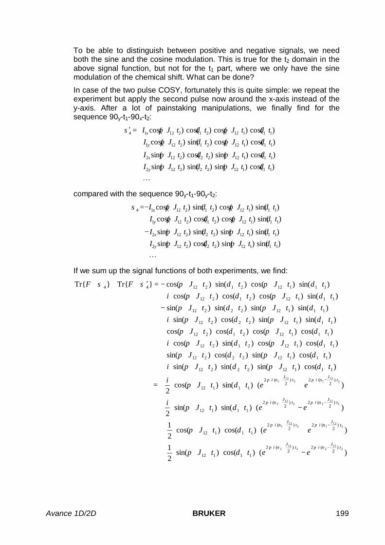
Avance 1D/2D BRUKER 199
To be able to distinguish between positive and negative signals, we needboth the sine and the cosine modulation. This is true for the t2 domain in theabove signal function, but not for the t1 part, where we only have the sinemodulation of the chemical shift. What can be done?
In case of the two pulse COSY, fortunately this is quite simple: we repeat theexperiment but apply the second pulse now around the x-axis instead of they-axis. After a lot of painstaking manipulations, we finally find for thesequence 90y-t1-90x-t2:
L+⋅⋅⋅⋅⋅⋅⋅⋅⋅+⋅⋅⋅⋅⋅⋅⋅⋅⋅+⋅⋅⋅⋅⋅⋅⋅⋅⋅+⋅⋅⋅⋅⋅⋅⋅⋅⋅=′
)cos()sin()sin()sin()cos()sin()cos()sin(
)cos()cos()sin()cos()cos()cos()cos()cos(
11112222122
11112222122
11112212121
111122121214
ttJttJIttJttJI
ttJttJIttJttJI
y
x
y
x
δπδπδπδπδπδπδπδπσ
compared with the sequence 90y-t1-90y-t2:
L+⋅⋅⋅⋅⋅⋅⋅⋅⋅+⋅⋅⋅⋅⋅⋅⋅⋅⋅−⋅⋅⋅⋅⋅⋅⋅⋅⋅+⋅⋅⋅⋅⋅⋅⋅⋅⋅−=
)sin()sin()cos()sin()sin()sin()sin()sin(
)sin()cos()cos()cos()sin()cos()sin()cos(
11112222122
11112222122
11112212121
111122121214
ttJttJIttJttJI
ttJttJIttJttJI
y
x
y
x
δπδπδπδπδπδπδπδπσ
If we sum up the signal functions of both experiments, we find:
)()cos()sin(21
)()cos()cos(21
)()sin()sin(2
)()sin()cos(2
)cos()sin()sin()sin()cos()sin()cos()sin(
)cos()cos()sin()cos()cos()cos()cos()cos()sin()sin()cos()sin(
)sin()sin()sin()sin()sin()cos()cos()cos(
)sin()cos()sin()cos(TrTr
212
2212
2
212
1212
1
212
2212
2
212
1212
1
)2
(2)2
(2
11112
)2
(2)2
(2
11112
)2
(2)2
(2
11112
)2
(2)2
(2
11112
1111222212
1111222212
1111221212
1111221212
1111222212
1111222212
1111221212
111122121244
tJ
itJ
i
tJ
itJ
i
tJ
itJ
i
tJ
itJ
i
eettJ
eettJ
eettJi
eettJi
ttJttJittJttJ
ttJttJittJttJttJttJi
ttJttJttJttJi
ttJttJFF
⋅−⋅⋅⋅⋅+⋅⋅⋅
⋅−⋅⋅⋅⋅+⋅⋅⋅
⋅−⋅⋅⋅⋅+⋅⋅⋅
⋅−⋅⋅⋅⋅+⋅⋅⋅
++
−⋅⋅⋅⋅⋅⋅+
+⋅⋅⋅⋅⋅⋅+
−⋅⋅⋅⋅⋅⋅+
+⋅⋅⋅⋅⋅⋅=
⋅⋅⋅⋅⋅⋅⋅⋅⋅⋅+⋅⋅⋅⋅⋅⋅⋅⋅⋅+
⋅⋅⋅⋅⋅⋅⋅⋅⋅⋅+⋅⋅⋅⋅⋅⋅⋅⋅⋅+⋅⋅⋅⋅⋅⋅⋅⋅⋅⋅+
⋅⋅⋅⋅⋅⋅⋅⋅⋅−⋅⋅⋅⋅⋅⋅⋅⋅⋅⋅+
⋅⋅⋅⋅⋅⋅⋅⋅⋅−=′⋅+⋅
νπνπ
νπνπ
νπνπ
νπνπ
δπ
δπ
δπ
δπ
δπδπδπδπ
δπδπδπδπδπδπ
δπδπδπδπ
δπδπσσ

200 BRUKER Avance 1D/2D
Which can also be expressed as:
( )
)(
))sin()sin()cos()(sin(21
)(
)sin()cos()cos()cos(21TrTr
212
2212
2
212
1212
1
)2
(2)2
(2
1111211112
)2
(2)2
(2
111121111244
tJ
itJ
i
tJ
itJ
i
ee
ttJittJ
ee
ttJittJFF
⋅−⋅⋅⋅⋅+⋅⋅⋅
⋅−⋅⋅⋅⋅+⋅⋅⋅
++
−⋅
⋅⋅⋅⋅⋅+⋅⋅⋅⋅+
+⋅
⋅⋅⋅⋅⋅+⋅⋅⋅⋅=′⋅+⋅
νπνπ
νπνπ
δπδπ
δπδπσσ
The final result will then lead to:
)()(41
)()(41TrTr
212
2212
2112
1112
1
212
1212
1112
1112
1
)2
(2)2
(2)2
(2)2
(2
)2
(2)2
(2)2
(2)2
(2
44
tJ
itJ
itJ
itJ
i
tJ
itJ
itJ
itJ
i
eeee
eeeeFF
⋅−⋅⋅⋅⋅+⋅⋅⋅⋅−⋅⋅⋅⋅+⋅⋅⋅
⋅−⋅⋅⋅⋅+⋅⋅⋅⋅−⋅⋅⋅⋅+⋅⋅⋅++
−⋅−+
+⋅+=′⋅+⋅
νπνπνπνπ
νπνπνπνπσσ
After Fourier transform, we find an all positive diagonal peak multiplet and ananti-phase cross peak multiplet of four peaks each.

Avance 1D/2D BRUKER 201
22.11 Summary and Useful Formulae
22.11.1 Effects on Spins in the Product Operator FormalismEffect of pulses on magnetization:
ββββ
ββ
ββ
β
β
β
β
β
β
sincos
sincos
sincos
sincos
zyy
zxx
yy
xx
xzz
yzz
III
III
II
II
III
III
x
y
y
x
y
x
+ →− →
→ →
+ →
− →
If the flip angle β = 90° then:
zyx
yxz
II
IIxy
xy
m →
± →,
,
90,
,90
Effect of chemical shift on magnetization:
) sin() cos(
) sin() cos(
tItII
tItII
II
xytI
y
yxtI
x
ztI
z
z
z
z
δδδδ
δ
δ
δ
− →+ →
→
⋅⋅
⋅⋅
⋅⋅
Effect of scalar coupling on magnetization:
yxtIIJ
yx
xzytIIJ
zy
yzxtIIJ
zx
zxytIIJ
y
zyxtIIJ
x
ztIIJ
z
IIII
tJItJIIII
tJItJIIII
tJIItJII
tJIItJII
II
zz
zz
zz
zz
zz
zz
21 2
21
1211221 2
21
1211221 2
21
1221121 2
1
1221121 2
1
1 2
1
22
)sin()cos( 22
)sin()cos( 22
)sin( 2)cos(
)sin( 2)cos(
2112
2112
2112
2112
2112
2112
→⋅− →⋅+ →⋅
− →+ →
→
π
π
π
π
π
π
ππππππππ

202 BRUKER Avance 1D/2D
22.11.2 Mathematical RelationsThe Euler relations where used extensively in the previous paragraphs:
)(2
)sin(
)(21)cos(
)sin()cos(
)sin()cos(
titi
titi
ti
ti
eeit
eet
tite
tite
⋅⋅−⋅⋅
⋅⋅−⋅⋅
⋅⋅−
⋅⋅
−−=⋅
+=⋅
⋅⋅−⋅=⋅⋅+⋅=
ωω
ωω
ω
ω
ω
ω
ωωωω
Frequently used simplifications in 2D:
α
αααααα
⋅⋅−=⋅+−=⋅−⋅−=+⋅−
iei
iiiii
)sin(cossincossincos 2
)(21
)(21cos
)()( titi
ititii
ee
eeee
⋅−⋅+
⋅⋅⋅−⋅⋅⋅
+=
⋅+=⋅
αβαβ
βααβα
)(2
)(2
sin
)()( titi
ititii
eei
eeei
e
⋅−⋅+
⋅⋅⋅−⋅⋅⋅
−−=
⋅−−=⋅
αβαβ
βααβα
References:
O. W. Sørensen, G.W. Eich, M. H. Levitt, G. Bodenhausen, R. R. Ernst, Progres in NMRSpectroscopy, 16, 163 (1983).

Avance 1D/2D BRUKER 203
113C acquisition and processing 4513C NMR with 1H decoupling 4813C NMR without decoupling 451D HMQC acquisition parameters 661D HMQC processing parameters 661D HMQC pulse sequence 651D proton acquisition and processing 311H decoupling 90° pulse calibration 581H decoupling 90° pulse during 13C acquisition 541H/13C chemical shift correlation 191H/1H through bond chemical shift correlation 19
9
90 degree pulse 185
A
acquisition commands 20acquisition parameters 20acquisition parameters with gated and inverse gated
decoupling 70angular momentum 183antiphase coherences 93ased 18atma 25AU Programs 20autolock 28
B
B0 184baseline submenu 153basl 153baslpnts 153BIRD parameter optimization 122BIRD preparation 119BIRD-HMQC 19Bloch equations 183, 184Boltzman distribution 185browse the data set directories 20
C
C13CPD 19C13DEPT135 19C13DEPT45 19C13DEPT90 19C13GD 19calcphinv 123cholesterylacetate 45Cholesterylacetate 31classical description 183cnst# 23COLOC 19, 115COLOC acquisition parameters 116COLOC pulse sequence 115configure the routing 21
correlation spectroscopy via long-range coupling115
CORTAB 9COSY 19, 81, 196, 199COSY acquisition parameters 83COSY processing parameters 84COSY-45 pulse sequence 82COSY45SW 19COSYDQFPHSW 19COSYGPDFPHSW 19COSYGPSW 19coupling constants 14cross-relaxation 103CURPRIN 154
D
d# 22damaging the probehead 9dataset 17dataset related commands 20DECP90 acquisition parameters 56DECP90 processing parameters 57DECP90 pulse sequence 54define solvent parameters 21defplot 102density matrix 186DEPT 72DEPT acquisition parameters 74DEPT processing parameters 75DEPT pulse sequence 73DEPT135 19DEPT45 19DEPT90 19detection operator 194Double-Quantum Filtered COSY 86DQF-COSY 19, 86DQF-COSY Pulse Sequence (with gradients) 90DQF-COSY phase correction 87DQF-COSY Processing Parameters 87DQF-COSY Pulse Sequence 86DQF-COSY with gradients 89
E
eda 18edg 18edhead 21, 24edlist 150, 167edp 18edprosol 24edsolv 21elim 154eliminate datapoints 154energy level 185equilibrium matrix 186Ethylbenzene 39Euler relations 202evolution of spin systems in time 187

204 BRUKER Avance 1D/2D
experiment number 17experiment time estimation 21experiments, table of common - 19expno 17
F
FID and free induction decay 189FnMODE 24fq#list 139frequency list 139
G
gated 1H-decoupling 69Gauss 160gaussian envelope 163, 166gaussian pulse 163getprosol 24gp syntax 24gradshim 29graphical display of the current pulse program 21GRASP DQF-COSY acquisition parameters 90GRASP-DQF-COSY Pulse Sequence 90GRASP-HMBC 129GRASP-HMBC pulse sequence 131GRASP-HMQC 129GRASP-HMQC pulse sequence 130GRASP-HSQC 129gyromagnetic ratio 183
H
Hartmann-Hahn condition 99HCCOLOCSW 19HCCOSW 19HETCOR 19HETCORR 109heteronuclear (X, H) shift correlation 109heteronuclear J-coupling 109heteronuclear J-couplings 115Heteronuclear Multiple Bond Correlation 125heteronuclear multiple quantum coherence 125Heteronuclear Multiple Quantum Correlation 119heteronuclear multiple-quantum coherence 119Heteronuclear Single Quantum Correlation 131HMBC 19, 125HMBC acquisition parameters 126HMBC processing parameters 127HMBC pulse sequence 126HMQC 19, 119HMQC pulse sequence 120HMQC with BIRD acquisition parameters 121HMQC with BIRD processing parameters 122HMQC with BIRD pulse sequence 120HMQC, HMBC and HSQC acquisition parameters
132homonuclear Nuclear Overhauser effect 99HPPR 26HSQC 19, 129, 131HSQC pulse sequence with gradients 132
I
INEPT 131information on pulse program nomenclature 23information on pulse program parameters 23integration of spectra 37intrng 153INV4GPLPLRNDSW 19INV4LPLRNDSW 19INV4SW 19INVBSW 19inverse chemical shift correlation 119, 129inverse experiments 129inverse gated decoupling 69inversion recovery 149inversion recovery acquisition parameters 151inversion recovery processing parameters 152inversion recovery pulse sequence 150INVIGPPHSW 19
K
Karplus relation 15
L
Larmor frequency 184Larmor theorem 183lock parameters 21lock the spectrometer 28lockdisp 28long-range 1H-13C J-couplings 125long-range chemical shift correlation 125low power pulse calibration 42
M
magnetic moment 183magnitude COSY 81maximum power levels 9mixing period, NOESY 103mixing time optimization (NOESY) 105mixing time, ROESY 99MLEV-17 93MLEVPHSW 19multiefp 142
N
NOE 103, 137NOE Difference 137NOE difference acquisition parameters 140NOE difference parameter optimization 140NOE difference processing parameters 142NOE difference pulse sequence 138NOE quantitation 143noemul 139noemult 139NOESY 19, 103NOESY acquisition parameters 105NOESY processing parameters 106NOESY pulse sequence 104NOESYPHSW 19Nuclear Overhauser effect 99

Avance 1D/2D BRUKER 205
Nuclear Overhauser Effect 103, 137Nuclear Overhauser Effect Spectroscopy 103
O
observable operators 189observable signals 189one-spin system 185
P
p# 22paropt 41phase correction (1D) 35phase cycling 159pl# 22population 185power level 9predefined parameter set 18preirradiation 137probehead 190proc_t1 152processing commands 20processing number 17processing parameters 21processing size 34procno 17PROTON 19pulse calibration for protons 39pulse calibration: carbon 51pulse program display 21pulse program information 20pulse program nomenclature 23pulse program parameters 22pulse sequence with gated 1H decoupling 69
R
read shim values 21receiver coil 184receiver gain adjustment (auto) 21recovery time values list 150relaxation 149restore eliminated datapoints 154RF-pulses 184RF-Pulses 186ROE 99ROESY 19, 99ROESY acquisition parameters 100ROESY processing parameters 101ROESY pulse sequence 99ROESYPHSW 19rotating coordinate system 186rotating frame 186Rotating-frame Overhauser Effect SpectroscopY 99rpar 18rstp 154
S
save shim values 21search for a specific dataset 20selco 161
selective COSY 163selective COSY acquisition parameters 165selective COSY pulse sequence 164selective excitation 159selective irradiation 163selective one-pulse sequence 160selective pulse 159selective pulse calibration 159selective TOCSY 166selective TOCSY acquisition parameters 168selective TOCSY processing parameters 169selective TOCSY pulse sequence 167selmlzf 161selzg 161setti 72shape tool 21shaped pulses 160Shapes 160shimming the sample 29single-quantum magnetization 131solvent parameters 21sp# 22spin 183spin-lattice relaxation 149spin-lock 99spinning 82stacked plot 155stackpar 156stackplot 155stdisp 160stop the acquisition 21
T
T1 calculation (AU program) 152T1 curves 154T1 measurement 149T1 parameters 155T1 relaxation 149t1bas 153t1delay 150, 154t1reg 153temperature control window 21The Hamiltonian 187thermal equilibrium 185time domain 34time units in XWinNMR 23title for a spectrum 72TOCSY 19TOCSY acquisition parameters 94TOCSY processing parameters 95TOCSY pulse sequence 93total correlation spectroscopy 93transmitter 184tuning and matching the probe 24
V
variable delay list 167vd 167vdlist 150

206 BRUKER Avance 1D/2D
W
weak coupling 193window function 35wobbling 21, 26, 27wobbling channel selection 21wpar 18
X
XHCORR 109XHCORR acquisition parameters 111XHCORR processing parameters 112XHCORR pulse sequence 110
Z
z-gradient hardware 19