auv thesis revision#1 with matlab - 123seminarsonly.com · 2013-01-05 · as autonomous underwater...

NAVAL POSTGRADUATE SCHOOL Monterey, California

THESIS

Approved for public release; distribution is unlimited.

LOITERING BEHAVIORS OF AUTONOMOUS

UNDERWATER VEHICLES by

Douglas L. Williams

June 2002

Thesis Advisor: Anthony J. Healey

THIS PAGE INTENTIONALLY LEFT BLANK

i

REPORT DOCUMENTATION PAGE Form Approved OMB No. 0704-0188 Public reporting burden for this collection of information is estimated to average 1 hour per response, including the time for reviewing instruction, searching existing data sources, gathering and maintaining the data needed, and completing and reviewing the collection of information. Send comments regarding this burden estimate or any other aspect of this collection of information, including suggestions for reducing this burden, to Washington headquarters Services, Directorate for Information Operations and Reports, 1215 Jefferson Davis Highway, Suite 1204, Arlington, VA 22202-4302, and to the Office of Management and Budget, Paperwork Reduction Project (0704-0188) Washington DC 20503. 1. AGENCY USE ONLY (Leave blank)

2. REPORT DATE June 2002

3. REPORT TYPE AND DATES COVERED Master’s Thesis

4. TITLE AND SUBTITLE: Loitering Behaviors of Autonomous Underwater Vehicles

6. AUTHOR(S) Douglas L. Williams

5. FUNDING NUMBERS

7. PERFORMING ORGANIZATION NAME(S) AND ADDRESS(ES) Naval Postgraduate School Monterey, CA 93943-5000

8. PERFORMING ORGANIZATION REPORT NUMBER

9. SPONSORING / MONITORING AGENCY NAME(S) AND ADDRESS(ES) N/A

10. SPONSORING / MONITORING AGENCY REPORT NUMBER

11. SUPPLEMENTARY NOTES The views expressed in this thesis are those of the author and do not reflect the official policy or position of the Department of Defense or the U.S. Government. 12a. DISTRIBUTION / AVAILABILITY STATEMENT Approved for public release; distribution is unlimited.

12b. DISTRIBUTION CODE

13. ABSTRACT In multi-vehicle mine hunting operations, it will be necessary at times for one vehicle to loiter at some point while

gathering communications of data from other vehicles. The loitering behaviors of the ARIES Autonomous Underwater Vehicle have never been completely defined. The track that the vehicle chooses to maintain station while circling around one specific point for an extended period of time may be sometimes random and unpredictable, unless defined in terms of specific tracks. Simulations were run and analyzed for various conditions to record the tendencies of the vehicle during different current conditions and approach situations. The stability of the Heading Controller was then analyzed in order to predict the position where the Line of Sight Guidance algorithm becomes unstable. The data obtained through the simulations supports and explains the tendencies ARIES exhibits while circling around a loiter point.

15. NUMBER OF PAGES

72

14. SUBJECT TERMS: Autonomous Underwater Vehicles, Robotics, Loitering Behavior, Line of Sight Guidance Instability, Liapunov Stability/Instability Theorem

16. PRICE CODE

17. SECURITY CLASSIFICATION OF REPORT

Unclassified

18. SECURITY CLASSIFICATION OF THIS PAGE

Unclassified

19. SECURITY CLASSIFICATION OF ABSTRACT

Unclassified

20. LIMITATION OF ABSTRACT

UL

NSN 7540-01-280-5500 Standard Form 298 (Rev. 2-89) Prescribed by ANSI Std. 239-18

ii


iii

Approved for public release; distribution is unlimited.

LOITERING BEHAVIOR OF AUTONOMOUS UNDERWATER VEHICLES

Douglas L. Williams Lieutenant, United States Navy

B.S., United States Naval Academy, 1995

Submitted in partial fulfillment of the

requirements for the degree of

MASTER OF SCIENCE IN MECHANICAL ENGINEERING

from the

NAVAL POSTGRADUATE SCHOOL

June 2002

Author: Douglas L. Williams

Approved by: Anthony J. Healey

Thesis Advisor

Terry R. McNelley, Chairman Department of Mechanical Engineering

iv


v

ABSTRACT

In multi-vehicle mine hunting operations, it will be necessary at times for one

vehicle to loiter at some point while gathering communications of data from other

vehicles. The loitering behaviors of the ARIES Autonomous Underwater Vehicle have

never been completely defined. The track that the vehicle chooses to maintain station

while circling around one specific point for an extended period of time may be sometimes

random and unpredictable, unless defined in terms of specific tracks. Simulations were

run and analyzed for various conditions to record the tendencies of the vehicle during

different current conditions and approach situations. The stability of the Heading

Controller was then analyzed in order to predict the position where the Line of Sight

Guidance algorithm becomes unstable. The data obtained through the simulations

supports and explains the tendencies ARIES exhibits while circling around a loiter point.

vi


vii

TABLE OF CONTENTS I. INTRODUCTION....................................................................................................... 1

A. BACKGROUND.............................................................................................. 1 B. SCOPE OF THIS WORK .............................................................................. 2

II. GENERAL BACKGROUND ON THE ARIES AUV ............................................. 3 A. VEHICLE DESCRIPTION............................................................................ 3 B. COMPUTER HARDWARE .......................................................................... 6 C. COMPUTER SOFTWARE............................................................................ 6

1. Architecture ......................................................................................... 6 2. Mission Control Modes....................................................................... 8

D. AUTO PILOT CONTROL LAWS................................................................ 8 1. Depth Controller ................................................................................. 8 2. Altitude Controller.............................................................................. 9 3. Heading Controller ........................................................................... 10 4. Cross Track Error Controller.......................................................... 10 5. Line of Sight Controller.................................................................... 13

E. NAVIGATION .............................................................................................. 14

III. LOITERING PARAMETERS AND IMPLEMENTATION................................ 19 A. GENERAL THEORY................................................................................... 19 B. LOITER POINT MAPPING........................................................................ 20

IV. LOITERING SIMULATIONS..................................................................................... 23 A. MATLAB SIMULATIONS WITH NO CURRENT.................................. 23 B. MATLAB SIMULATIONS WITH CURRENT......................................... 25

1. Current Condition Simulation #1 .................................................... 25 2. Current Condition Simulation #2 .................................................... 32 3. Current Condition Simulation #3 .................................................... 36 4. Current Condition Simulation #4 .................................................... 39 5. Current Condition Simulation #5 .................................................... 41 6. Current Condition Simulation #6 .................................................... 42 7. Current Condition Simulation #7 .................................................... 44 8. Current Condition Simulation #8 .................................................... 46

V. DISCUSSION OF RESULTS......................................................................................... 49 A. RELATION BETWEEN APPROACH AND CURRENT

DIRECTION.................................................................................................. 49 B. LINE OF SIGHT GUIDANCE INSTABILITY......................................... 50

VI. STABILITY ANALYSIS .............................................................................................. 55 A. LIAPUNOV STABILITY/INSTABILITY THEOREMS ......................... 55

VII. CONCLUSIONS AND RECOMMENDATIONS..................................................... 59

APPENDIX A. MATLAB FILES FOR AUV LOITERING ............................................. 61

APPENDIX B. MATLAB FILES FOR AUV LOITERING ............................................. 63

APPENDIX C. MATLAB FILES FOR AUV LOITERING ............................................. 65

viii

APPENDIX D. MATLAB FILES FOR AUV LOITERING ............................................. 67

LIST OF REFERENCES ..................................................................................................... 69

INITIAL DISTRIBUTION LIST ........................................................................................ 71

ix

ACKNOWLEDGMENTS

This work is done within the general support of funds from the Office of Naval

Research. I would like to acknowledge Professor Tony Healey for his guidance, patience

and motivation throughout the thesis process. His high level of technical competence and

uncanny ability to teach provided me with a great understanding of the subject area.

Additionally, I would like to thank LCDR John Keegan and LT Joseph Keller for their

assistance and support in obtaining and interpreting data for this thesis. Finally and most

importantly I would like to thank my wife, Tammy, for her love and support.

x


1

I. INTRODUCTION

A. BACKGROUND

As Autonomous Underwater Vehicle (AUV) technology advances, mission

objectives in a military environment will become more enhanced. Specifically, minefield

mapping and mine reconnaissance scenarios will utilize AUVs in order to ensure

personnel safety. As the possibility of military conflict continues throughout the world,

the need for capable mission objectives for AUVs becomes imperative. AUVs will be

involved with complex and dynamic mission assignments where data exchange between

vehicles occurs frequently and objectives can change often.

A loitering technique will be introduced in a vehicle’s mission capabilities to

attempt to increase an AUV system objective capabilities. This will allow the vehicle to

perform in a dynamic environment where data exchanges and changing mission

objectives are to be completed. Loitering parameters will be introduced in the

programming of the mission and will be executed upon a transition criteria being met.

Such criteria are listed:

1. Receiving a command from the control station to proceed to a loiter station for data transfer or for further tasking parameters.

2. Upon mission abort from time out procedures or any other abort parameters with the exception of immediate surfacing abort criteria.

3. Upon completion of current mission assignment.

Loitering stations will be defined and introduced into the mission assignment

through coding prior to the execution of the mission. There will be a specific loiter

station for each leg of the AUV’s defined track. If the AUV meets the criteria listed

above, it will proceed to the defined loiter station for the respective leg and wait further

instructions.

Before being able to test loitering missions with the AUV, modeling of the

vehicle must be researched to accurately to predict vehicle characteristics during such

assignments. Accurate guidance calculations become imperative in order to accomplish

2

the dynamic mission parameters set forth. The vehicle must reach its intended loiter

point and maintain station until further instructions are received. Also, the effect of

hydrodynamic forces such as waves and currents acting on the vehicle must be taken into

consideration when attempting to predict the tendencies of the vehicle proceeding and

maintaining position at a loiter station. If the vehicle cannot maintain station at a

loitering point due to the forces acting on it then a different stationing concept must be

conceived.

B. SCOPE OF THIS WORK

The loitering technique of the ARIES is not thoroughly understood. The vehicle

does not maintain station at one point very well. The track that the AUV follows during a

loiter maneuver is random and unpredictable. This thesis is written to break down the

reasons why ARIES performs in such a way and what alternatives can be made to prevent

such actions.

Chapter II will explain the general background data of ARIES. This will include

current command and control configuration, hardware and software architecture, and a

general explanation of the control laws that govern the vehicle’s movements.

Chapter III will discuss the theory and benefits behind the implementation of

loitering stations along each leg of a mine mapping mission. The parameters to transition

to a loiter station will also be discussed in detail.

Chapter IV will consists of simulation data that contains various conditions that

ARIES could encounter in an actual run. The simulations show the relevance of current

direction acting on the vehicle and which conditions are optimal for ARIES.

Chapter V will justify the reason for the loitering behavior that the AUV exhibits

when attempting to loiter around a point.

Chapter VI is a stability analysis that supports the theories that the Line of Sight

Guidance is unstable when approaching the loitering point.

Chapter VII discusses options to correct for the loitering behavior and other

alternatives to research in the future.

3

II. GENERAL BACKGROUND ON THE ARIES AUV

A. VEHICLE DESCRIPTION

(This section is largely taken from [1], but is repeated here for convenience of the

reader). Construction on ARIES began in the fall of 1999 and was fully operational in

the spring of 2000. The ARIES vehicle is a shallow water communications server

vehicle with a Differential Global Positioning System (DGPS) and a Doppler aided

Inertial Measurement Unit (IMU) / Compass navigation suite. Figure 1 shows the

command and control system as it exists today.

Figure 1. Current Command and Control. [1]

ARIES measures approximately 3 meters long, 0.4 meters wide, 0.25 meters high,

and weighs 225 kilograms. A fiberglass nose that becomes flooded is used to house the

external sensors, power switches, and status indicators. The hull is constructed of 0.25

4

inches thick 6061 aluminum that contains all the electronics, computers, and batteries.

The ARIES is powered by six 12-volt rechargeable lead acid batteries and the endurance

is approximately 3 hours at a top speed of 3.5 knots, or 20 hours hotel load only. ARIES

can operate safely at a depth of 30 meters, however, through finite element analysis it has

been shown through hull strengthening that ARIES can operate safely up to 100 meters.

Figure 2 shows the major hardware components of the ARIES.

Figure 2. Hardware Components. [1]

Propulsion is achieved using twin 0.5 Hp electric drive thrusters located at the

stern. Heading and depth is controlled using upper bow and stern rudders and a set of

bow and stern planes, respectively. Although not currently installed on ARIES, vertical

and lateral cross-body thrusters can be used to control surge, sway, heave, pitch, and yaw

motions during slow or zero speed maneuvers.

5

The navigation sensor suite consists of a 1200 kHz RD Instruments Navigator

Doppler Velocity Log (DVL) that also contains a TCM2 magnetic compass. This

navigation suite measures vehicle altitude, ground speed, and magnetic heading. Angular

rates and accelerations are measured using a Systron Donner 3-axis Motion Pak IMU.

While surfaced, differential GPS (Ashtech G12-Sensor [2]), accuracy 40 centimeters, is

available to correct any navigational errors accumulated during the submerged phases of

a mission. In addition, and because of inaccuracies in the TCM2 compass, a Honeywell

HMR3000 magnetic-restrictive compass, corrected by a deviation table, is used as the

primary heading reference standard. Experiments have shown that the deviation table

maximum error is approximately 4 degrees in some orientations.

A fixed wide-angle video camera (Deep Sea Power and Light – SS100) is located

in the nose and connected to a Digital Video Cassette (DVC) recorder. The computer is

interfaced to the recorder and controls the on/off and start/stop functions. The video

image has the date, time, position, depth, and altitude superimposed onto it.

A scanning sonar (Tritech ST725) or a profiling sonar (ST1000) is used for

obstacle avoidance and target acquisition/reacquisition. The sonar can scan continuously

through 360 degrees of rotation or be swept through a defined angular sector.

Freewave Radio Modems are used for moderate bandwidth (2000-3000 bytes/sec

over 4 to 6 nautical miles with repeaters) command and control (C2), between command

center and the vehicle when surfaced. Kermit file transfer protocol is used in the vehicle

computer with Zmodem through Procomm protocol on the base station side.

Experiments conducted have transferred data files between the surfaced ARIES, a Boston

Whaler repeater station, and a base station command center. Radio modem connections

require line-of-sight and are critically dependent on antennae height above ground.

ARIES has an FAU acoustic modem installed onboard, details of which are

provided in [3]. The successful operation of the modem is imperative if ARIES is to be

used as a network server. Other modems could be installed in the same fashion as the

FAU modem allowing for more than one modem to be used during the same mission.

This would allow future networking links between different vehicles without an

interoperable standard in place.

6

B. COMPUTER HARDWARE

The dual computer system unit consists of two Ampro Little Board 166 MHz

Pentium computers with 64 MB RAM, four serial ports, a network adapter, and a 2.5 GB

hard drive each. Two AC/DC voltage converters for powering both computer systems

and peripherals are integrated into the computer package. The entire computer system

draws a nominal 48-Watts. Both systems use TCP/IP sockets over thin wire Ethernet for

inter processor communications and connections to an external LAN. The sensor data

gathering computer is designated QNXT, while the second is named QNXE and executes

the various auto-pilots for servo level control. Both computers are used as the baseboard

for a stack of Diamond Systems PC-104 data acquisition boards.

C. COMPUTER SOFTWARE

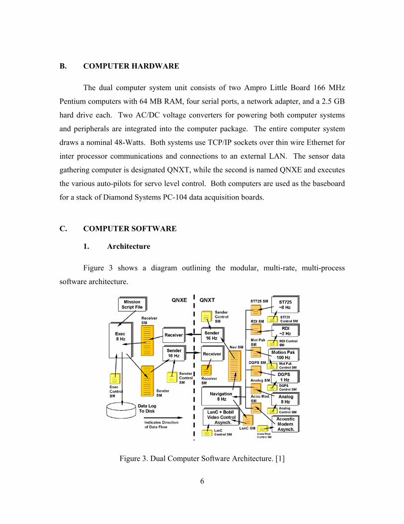
1. Architecture

Figure 3 shows a diagram outlining the modular, multi-rate, multi-process

software architecture.

Figure 3. Dual Computer Software Architecture. [1]

7

This scheme is designed to operate using a single computer processor, or two

independent cooperating processors linked through a network interface. Splitting the

processing between two computers can significantly improve computational load

balancing and software segregation. A dual computer implementation is presented here,

since, in the ARIES, each processor assumes different tasks for mission operation. Both

computers run the QNX real time operating system using synchronous socket sender and

receiver network processes for data sharing between the two. On each processor, inter-

process communication is achieved using semaphore controlled shared memory

structures. Deadlocks and race conditions are explicitly eliminated by the careful use of

semaphores in this system design. AT boot time, the network processes are started

automatically and all shared memory segments are created in order to minimize the

amount of manual setup performed by the user.

All vehicle sensors are interrogated by separate, independently controlled,

concurrent processes, and there is no restriction on whether the processes operate

synchronously or asynchronously. Since various sensors gather data at different rates,

each process may be tailored to operate at the acquisition speed of the respective sensor.

Each process may be started, stopped, or reset independently allowing easy

reconfiguration of the sensor suite needed for a given mission. All processes are written

in C.

To allow synchronous sensor fusion, each process contains a unique shared

memory data structure that is updated at the specific rate of each sensor. All sensor data

are accessible to a synchronous navigation process through shared memory and is a main

feature of the software architecture. Incorporated into the navigation process is an

extended Kalman filter that fuses all sensor data and computes the real time position,

orientation, velocity, etc, of the vehicle. The dual compute implementation uses one

processor for data gathering and running the navigation filters, while the second uses the

output from the filters to operate the various auto-pilots for servo level control. Once the

state information is computed, it is transmitted to the second computer over standard

TCP/IP sockets.

8

2. Mission Control Modes

Vehicle behaviors are determined by a pre-programmed mission script file. This

is parsed in the QNXE computer by the processes Exec. The file contains a sequential

list of commands that the vehicle is to follow during a mission. These commands may be

as simple as setting the stern propulsion thruster speeds, to more complex maneuvers

such as commanding the vehicle to repeatedly fly over a submerged target at a given GPS

coordinate using altitude and cross-track error control.

D. AUTO PILOT CONTROL LAWS

The ARIES uses four different auto pilots for flight maneuvering control. They

consist of independent diving, steering, altitude above bottom, and cross-track error

controllers. All four auto pilots are based on sliding mode control theory and each mode

(i.e. diving, steering, etc) is de-coupled for ease of implementation and design. A

reference for the details of controller design methodology may be found in (Healey and

Lienard, 1993, [4]). The designers of the ARIES have found that Sliding Mode

controllers are more simple to use and implement with minimal tuning than PID, LQR,

fuzzy and heuristic control.

1. Depth Controller

Since the vehicle depth can be independently controlled by the dive planes alone,

the diving controller may be modeled by a linearized system with a single generalized

input control, u(t), generating a pitch-dive control distributed to bow and stern planes in

an equal and opposite amount, and is of the form

ub Axx += , (1)

and for the ARIES, the dynamics are given by the system of equations

)( )(006091.2

)()()(

0000100032.03899.1

)()()(

disturttZttq

UtZttq

sp +

−+

−

−−=

δθθ

(2)

9

where, )(tq is the pitch rate, )(tθ is the pitch angle, )(tZ is the depth in meters, and

)(tspδ is the stern plane angle in radians. U is the nominal longitudinal speed of the

vehicle expressed in (m/sec) and a value of 1.8 m/sec is used. Although the bow and stern

planes may be independently controlled, currently both sets of planes operate as coupled

pairs such that the command to the bow planes is )(tspδ− . Notice that the heave

velocity, w, equation is ignored, as also are its effects on the q and Z equations of motion.

They are considered to be disturbances. The reduction of the system to third order

creates a simplification that is both valid and useful.

The sliding surface is then formed as a linear combination of state variable errors

in the usual way. Ignoring any non-zero pitch angle and rate commands, the sliding

surface polynomial becomes

))(( )()()( t Z Z072488.0 tθ6385.0 tq7693.0 tσ com −++= (3)

and the corresponding control law for the stern planes is

))(()()(()( φσ /ttanh η tθ1086.0 tq4105.0 -4994.0 tδsp ++= (4)

where, 0.1 =η and 5.0 =φ .

2. Altitude Controller

In order to control the vehicle altitude above the bottom designated )(th , we

simply need to change some of the signs of the terms from the diving equations. Noting

the sign difference of the pitch angle and rate coefficients, this results in the following

sliding surface

t h h0724.0 tθ6385.0 tq7693.0 - tσ com ))(()()()( −+−= (5)

The stern plane command for altitude control is

)))/((t )( )( (- )( φσηθδ tanht1086.0tq4105.04994.0tsp +−= (6)

where, 0.1 =η , 5.0 =φ , and )(th in meters replaces the vehicle depth, Z.

10

3. Heading Controller

By similar reasoning, and to eliminate the need to feedback the sideslip velocity,

we argue that a second order model is sufficient. The side-slip effects are treated as

disturbances that the control overcomes. Thus, the heading model becomes

)( )()( )( )( )(

trtesdisturbanctbtartr r

=++=

ψδ

(7)

where, )(tr is the yaw rate and )(trδ is the stern rudder angle. The coefficients a and b

have been determined using system identification techniques from past in water

experiments and are 30.0 a −= rad/sec and 1125.0 b −= rad/sec2. The stern and bow

rudders operate in the same way as the planes, therefore, the command to the bow rudder

is )(trδ− .

Notice that in order to use this steering law, ) - ( ψψ com must lie between 0180 ± ,

and is de-wrapped as needed in order to make that happen, and ignoring any non-zero

command yaw rate, the sliding surface is defined by

))( - ( )( - )( t1701.0tr9499.0t com ψψσ += (8)

The stern rudder command for heading control is

)))/(()((- )( φσδ ttanh η tr5394.2543.1tr += (9)

where, 0.1 =η and 5.0 =φ .

4. Cross Track Error Controller

To follow a set of straight line tracks that form the basis of many guidance

requirements, a sliding mode controller is presented that has been experimentally

validated under a wide variety of conditions. Other works have studied this problem for

land robots, (for example, Kanayama, 1990) and usually develop a stable guidance law

based on cross track error. Here, with Figure 4 as a guide to the definitions, we use a

combination of a Line of Sight Guidance (Healey, Lienard, 1993) and a Cross Track

Error Control for situations where the vehicle to track heading error is less than 40

11

degrees. For the line of sight guidance with large heading error, a separate line of sight

controller is used.

One of the shortcomings of the heading controller defined above is that it has no

ability to track a straight line path between two way points since it can only regulate the

vehicle heading. It is desired to command the vehicle to track a line between two way

points with both a minimum of error from the track and heading error between the

vehicle and the track. This type of regulation is known as cross track error control and

the variable definitions are illustrated in Figure 4.

Figure 4. Cross Track Error Definitions. [1]

The variable of interest to minimize is the cross track error, )(tε , and is defined

as the perpendicular distance between the center of the vehicle (located at ( )( ),( tYtX )

and the adjacent track line. The total track length between way point i and i-1 is given by

22 ) () ( )1i(wpt)i(wpt)1i(wpt)i(wpti YY XX L −− −+−= (10)

where, the ordered pairs ) ( )i(wpt)i(wpt Y,X and ) ( )1i(wpt)1i(wpt X,Y −− are the current and

previous way points respectively. The track angle, )(itrkψ , is defined by

12

) , (tan )1()()1()(1

)( −− −−= iwptiwptiwptiwpt-

itrk XXYY ψ (11)

The cross track heading error )i(CTEt~ )(ψ for the ith segment is defined as

)()( )( )(~itrkiCTE tt ψψψ −= (12)

where, )()( iCTEt~ψ must be normalized to lie between 0180 ± . The difference between the

current vehicle position and the next way point is

)()(

)( )(

t Y Y tY~t X XtX~

wpt(i)wpt(i)

wpt(i)wpt(i)

−=

−= (13)

With the above definitions, the distance to the ith way point projected to the track

line itS )( , can be calculated using

i)1i(wpt)i(wpt)i(wpt)1i(wpt)i(wpt)i(wpti /LYYtY~ XXtX~tS ) ( )() ()( )( −− −+−= (14)

therefore, itS )( ranges from 0-100% of iL .

The cross track error )(tε may now be defined as

))(()()( tδsint S t pi=ε (15)

where, )(tδp is the angle between the line of sight to the next way point and the current

track line given by

))(~ )(~(tan

) , (tan)(

)()(1

)1()()1()(1

iwptiwpt-

iwptiwptiwptiwpt-

p

tXtY

XXYY tδ

−−

−−= −− (16)

and must be normalized to lie between 0180 ± .

With the cross track error defined, the sliding surface can be cast in terms of

derivatives of the errors such that

))(()( ))(()( )(

))(()( )())(( )(

)( )(

)()(

)(

)(

iCTE2

iCTE

iCTE

iCTE

t~sintUrt~costrUt

t~costUrtt~sinUt

tt

ψψε

ψεψε

εε

−=

=

==

13

The sliding surface for the cross track error controller becomes a second order

polynomial of the form

)( )( )( )( tttt 21 ελελεσ ++= (17)

The condition for stability of the sliding mode controller is

)/(- )( )( )( )( φσηελελεσ =++= tttt 21 (18)

and to recover the input for control, the heading dynamics Equation (7) may be

substituted into Equation (16) to obtain

))(( ))(()( ))(()( ))(() )((

)(

)()()(

iCTE2

iCTE1iCTE2

iCTEr

t~sinUt~costUrt~sintUrt~cosbtarU

ψλψλψψδ

+

+−+

(19)

Rewriting Equation (15), the sliding surface becomes

)( ))(( ))(()( )( )()( ttψ~sinUtψ~cost U rt 2iCTE1iCTE ελλσ ++= (20)

The rudder input can be expressed as

)))/(( ))(( ))(()( ))(())((

))(()(())((

)(

)(

)()(

)()(

φσλλ

δ

tηtψ~sinU tψ~costUrtψ~sintrU

tψ~costUartψ~cosUb

1 t

iCTE2

iCTE1iCTE2

iCTEiCTE

r

−−

−+

−

=

(21)

where, 6.0 1 =λ , 1.0 2 =λ , 1.0 =η , and 5.0 =φ . To avoid division by zero, in the

rare case where 0.0 tψ~cos CTE =))(( (i.e. the vehicle heading is perpendicular to the track

line) the rudder command is set to zero since this condition is transient in nature.

5. Line of Sight Controller

When the condition arises that the magnitude of the cross track heading error

)()( iCTEtψ~ exceeds 400, a Line of Sight Control (LOS) is used. In this situation, the

heading command can be determined from

))(~,)(~(tan )( )()(1

)( iwptiwpt-

LOScom tXtYt =ψ (22)

14

and the LOS error from

)( )( )( ttt~)LOS(comLOS ψψψ −= (23)

and the control laws used for heading control, Equations (8,9) may be used.

Two conditions may be true for the waypoint index to be incremented. The first

and most usual case is if the vehicle has penetrated the way point watch radius )i(wR .

Secondly, if a large amount of cross track error is present, the next way point will become

active if the projected distance to the way point itS )( reached some minimum value

)(iminS , such that

( ) THEN )())(())(( )()()()( S t S|| R tY~ tX~if iminiiw2

iwpt2

iwpt <≤+

Activate Next Way Point

In water experimental results using the controllers presented above will now be

presented in the next section.

E. NAVIGATION

The ARIES vehicle uses an INS / DOPPLER / DGPS navigational suite and an

Extended Kalman Filter (EKF) which was developed and presented in ([5] and [6]), and

may be tuned for optimal performance given a set of data. The main impediments to

navigational accuracy are the heading reference and the speed over ground measurement.

In this system, the heading reference is derived from both the Honeywell compass and

the Systron Donner IMU, which provides yaw rate. The fusion of the yaw rate and the

compass data leads to an identification of the yaw rate bias, which is assumed to be a

constant value. The compass bias, which is mostly dependent on vehicle heading relative

to magnetic north, is identified in the EKF ([6]), using DGPS positions when surfaced.

When submerged, the position error covariance grows, but is corrected on surfacing. A

relatively short surface time, (for example, 10 seconds) allows the filter to re-estimate

biases, correct position estimates and continue with improved accuracy. As a

demonstration, the ARIES vehicle was operated in Monterey Bay, in a series of runs

15

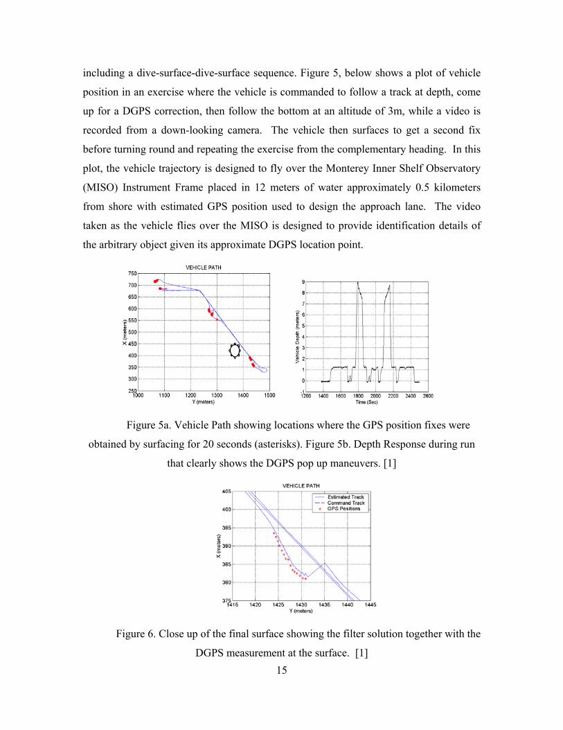
including a dive-surface-dive-surface sequence. Figure 5, below shows a plot of vehicle

position in an exercise where the vehicle is commanded to follow a track at depth, come

up for a DGPS correction, then follow the bottom at an altitude of 3m, while a video is

recorded from a down-looking camera. The vehicle then surfaces to get a second fix

before turning round and repeating the exercise from the complementary heading. In this

plot, the vehicle trajectory is designed to fly over the Monterey Inner Shelf Observatory

(MISO) Instrument Frame placed in 12 meters of water approximately 0.5 kilometers

from shore with estimated GPS position used to design the approach lane. The video

taken as the vehicle flies over the MISO is designed to provide identification details of

the arbitrary object given its approximate DGPS location point.

Figure 5a. Vehicle Path showing locations where the GPS position fixes were

obtained by surfacing for 20 seconds (asterisks). Figure 5b. Depth Response during run

that clearly shows the DGPS pop up maneuvers. [1]

Figure 6. Close up of the final surface showing the filter solution together with the

DGPS measurement at the surface. [1]

16

In Figure 6, a close up of the final surfacing maneuver shows that there is great

consistency in estimating the true DGPS data point as seen by the AshTec G-12 unit on

board. The difference between the Kalman Filter solution and the DGPS data points

while surfaced is sub meter precision. However, the difference between the dead

reckoning solution underwater is a few meters off the mark.

In Figure 7, the number of visible satellite vehicles seen by the DGPS unit are

shown to evolve quickly. Within 10 seconds, 9 satellites are being used to compute the

position solution.

Figure 7. Time History of the response of the number of visible GPS satellites

during the surface phase shown in Figure 6. [1]

Figure 8. Compass Bias Estimate versus Time. [1]

17

Figure 8 shows the response of the heading bias estimate from the EKF for the

entire run. At each surface approximately 10 DGPS points are obtained which rapidly

corrects the compass bias. However, as is seen, compass corrections in the neighborhood

of 5 degrees are still needed to predict correctly the vehicle positions. This is an

indication that further corrections of the compass deviation table are needed. The

remaining question is whether or not the deviations are predictable or random. While

some additional runs suggest that there may be some degree of consistency, it remains to

be shown conclusively.

18


19

III. LOITERING PARAMETERS AND IMPLEMENTATION

A. GENERAL THEORY

As discussed earlier, a series of parameters must be met before the ARIES can

transition to a loiter point. Figure 9 gives a graphic description of the transitions that

must occur.

Time Out

Time Out

Transition Transition

Figure 9. Loiter Logic. [7]

If the ARIES “times out” prior to reaching the next waypoint, meaning the AUV

does not reach the next waypoint in the allotted amount of time, or if the vehicle receives

a command (CMD) from the controlling station, the vehicle will proceed to the respective

loiter point, depending on the leg that ARIES is on. Normally the AUV aborts its

mission completely if there is “time out” prior to reaching the next intended waypoint.

Having the vehicle proceed to a loiter point instead of aborting the entire mission allows

the vehicle to maintain station at the loiter point and receive new mission parameters

and/or commands from the control station instead of aborting the entire mission all

together. If the criteria set forth for transition to the next waypoint is met, the vehicle

will proceed as programmed until commanded by the control station to proceed to a loiter

point. This logic allows flexibility for the vehicle to continue on its mission until the

control station requires it to break off its pre-programmed track because of possible

rendezvous with another vehicle for data transfer or adjusting mission parameters.

Start Way Point

#1

Loiter #2

CMD CMD

Loiter#1

Way Point

#2

20

B. LOITER POINT MAPPING

Generally, for a given mine mapping mission, the vehicle will have a series of

tracks to follow in sequence termed “legs”. Figure 10 below is a typical diagram of the

legs ARIES would follow for a mine mapping mission.

Figure 10. Typical Legs for a Mine Mapping Mission.

The idea for implementing loitering with the ARIES is to have pre-programmed

loiter points within the program itself. More specifically, each leg would have a specific

loiter point designated to it. As the ARIES travels down each leg, there is a respective

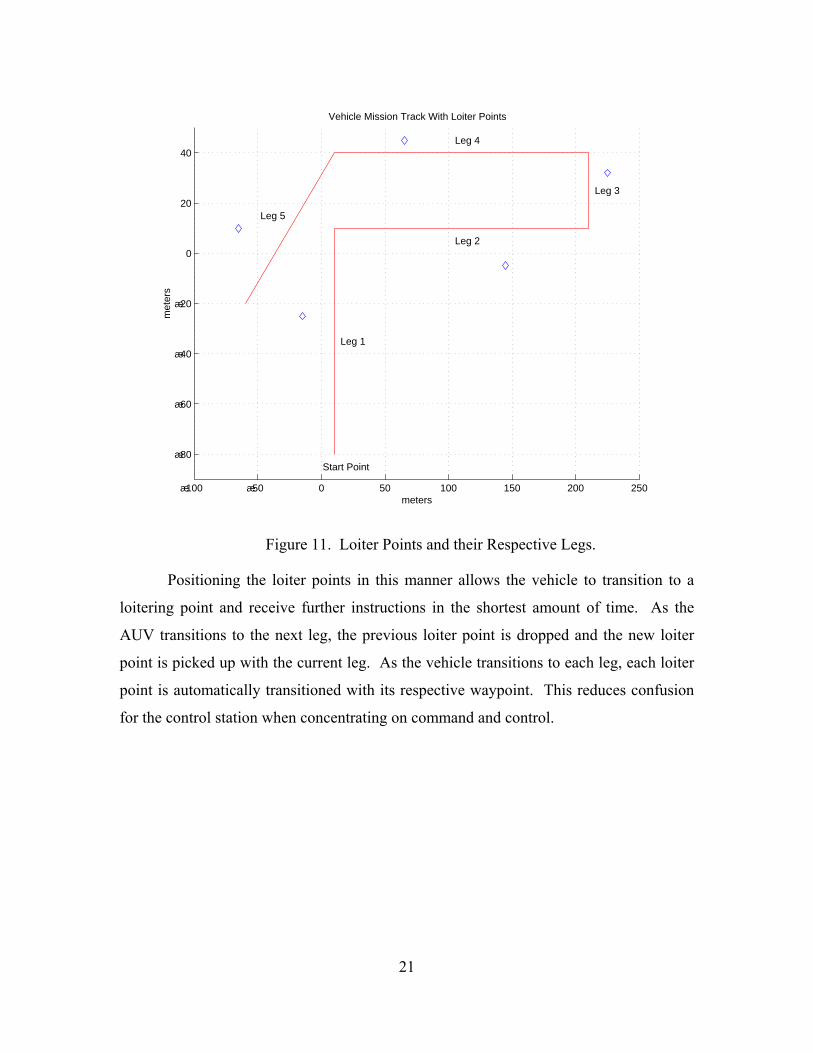
loiter point attached to the leg. Figure 11 gives a graphical description of the loiter points

and their respective legs. Note that the position of the loiter points are arbitrary and

should be determined by the programmer according to the mission objectives and

parameters.

−100 −50 0 50 100 150 200 250

−80

−60

−40

−20

0

20

40

Vehicle Mission Track

meters

met

ers

Start Point

Leg 1

Leg 2

Leg 3

Leg 4

Leg 5

21

Figure 11. Loiter Points and their Respective Legs.

Positioning the loiter points in this manner allows the vehicle to transition to a

loitering point and receive further instructions in the shortest amount of time. As the

AUV transitions to the next leg, the previous loiter point is dropped and the new loiter

point is picked up with the current leg. As the vehicle transitions to each leg, each loiter

point is automatically transitioned with its respective waypoint. This reduces confusion

for the control station when concentrating on command and control.

−100 −50 0 50 100 150 200 250

−80

−60

−40

−20

0

20

40

Vehicle Mission Track With Loiter Points

meters

met

ers

Start Point

Leg 1

Leg 2

Leg 3

Leg 4

Leg 5

22


23

IV. LOITERING SIMULATIONS

A. MATLAB SIMULATIONS WITH NO CURRENT

A MATLAB program was modified to include a loiter point on the first leg of the

track. At an arbitrary time along the first leg, the operator is given a choice to proceed to

Loiter Point 1 or continue on track. Under real operating conditions the AUV would be

interrupted during its mission and commanded to a respective loiter point. However,

since MATLAB is not a real time operating program the program itself had to be

interrupted to interpret the operator’s intentions. Below is a figure that shows what was

explained above.

Figure 12. Arbitrary Position Along Track AUV is Ordered to Loiter Point.

The simulation has an input break built into the program to find the operator’s

intentions. At this point the operator either chooses to continue on track or to proceed to

Vehicle commanded to proceed to loiter point

24

a loiter point. The next figure shows the vehicle as it is commanded to proceed to a loiter

point.

Figure 13. Vehicle Characteristics During a Loiter of 62 seconds.

Once the vehicle is commanded to proceed to the loiter point, it uses its normal

Line of Sight and Cross Track Error guidance to proceed to the loiter point. The watch

radius around the loiter point is set to zero so that the ARIES “never reaches” the point

and thus, continues to circle or loiter. Figure 13 shows that ARIES maintains a tight

bounded circular shape around the point of approximately 20 meters in diameter. As the

AUV continues to loiter it should report its GPS position every 10 – 15 minutes to the

control station in order to update the operators and correct itself for position errors. As

ARIES is in the loiter, the control station can determine what and if mission parameters

need to be changed such as, rendezvous with another vehicle, change the current track, or

continue on the original track.

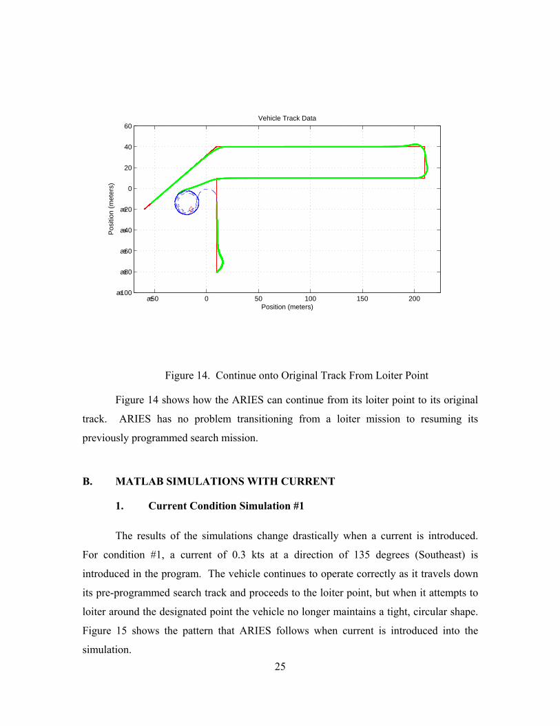
Figure 14 is a simulation that shows the vehicle as it continues from its loiter

point back to the original track.

−50 0 50 100 150 200−100

−80

−60

−40

−20

0

20

40

60Vehicle Track Data

Pos

ition

(m

eter

s)

Position (meters)

25

Figure 14. Continue onto Original Track From Loiter Point

Figure 14 shows how the ARIES can continue from its loiter point to its original

track. ARIES has no problem transitioning from a loiter mission to resuming its

previously programmed search mission.

B. MATLAB SIMULATIONS WITH CURRENT

1. Current Condition Simulation #1

The results of the simulations change drastically when a current is introduced.

For condition #1, a current of 0.3 kts at a direction of 135 degrees (Southeast) is

introduced in the program. The vehicle continues to operate correctly as it travels down

its pre-programmed search track and proceeds to the loiter point, but when it attempts to

loiter around the designated point the vehicle no longer maintains a tight, circular shape.

Figure 15 shows the pattern that ARIES follows when current is introduced into the

simulation.

−50 0 50 100 150 200−100

−80

−60

−40

−20

0

20

40


Pos

ition

(m

eter

s)

Position (meters)

26

Figure 15. Loitering Track with Current for 25 seconds.

The parameters for the Figure 15 simulation has the vehicle proceeding to the

loiter point by making a heading change of approximately 90 degrees. The vehicle

circles around the loiter point for approximately 25 seconds. The current causes the

ARIES AUV to fall off its tight, circular pattern that we viewed in Figures 13 and 14.

The pattern is still somewhat circular in nature, but as ARIES continues to attempt to

drive over the loiter point, the vehicle’s track is slowly shifting to the south. Figure 16 is

a closer view of the vehicle’s track around the loiter point.

−50 0 50 100 150 200−100

−80

−60

−40

−20

0

20

40


Position (meters)

Pos

ition

(m

eter

s)

27

Figure 16. Close Up View of Vehicle Loiter Track After 25 Seconds with Current.

From Figure 16, it is observed that the vehicle proceeds to the loiter point as

commanded. Once it passes over the point it continues to circle because the loiter point

has a radius of zero, therefore, the vehicle never reaches the “waypoint” and continues to

try until it does. The set and drift of the current acts on the vehicle and the tight circular

shape that ARIES exhibited with no current is shifted in a southerly direction.

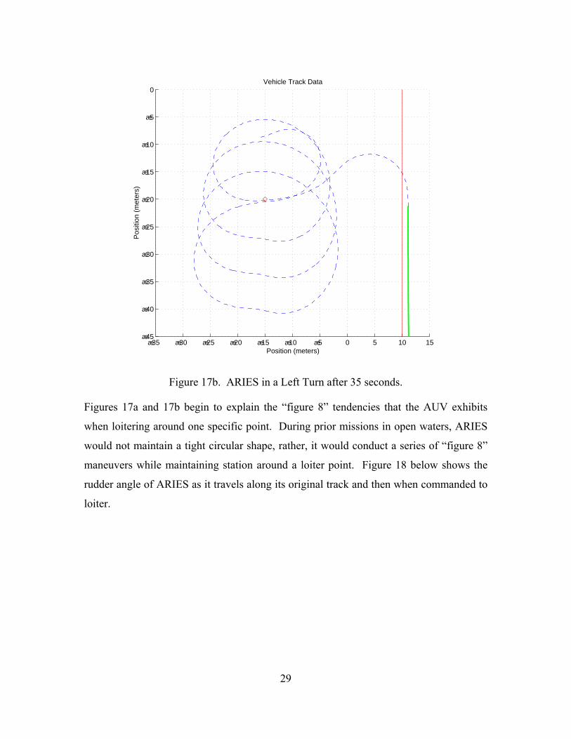
Figure 17a shows the vehicle track after 32 seconds. ARIES continues its circular

pattern with a series of right turns until it is too far south of the loiter point and shifts the

rudder. Now a circular pattern with a series of left turns exists. Figure 17b shows the

AUV at 35 seconds as it is in a series of left turns in its attempt to pass over the loiter

point.

−35 −30 −25 −20 −15 −10 −5 0 5 10 15−45

−40

−35

−30

−25

−20

−15

−10

−5

0Vehicle Track Data

Position (meters)

Pos

ition

(m

eter

s)

28

Figure 17a. ARIES is south of the loiter point and begins to make a left turn after 32

seconds.

−35 −30 −25 −20 −15 −10 −5 0 5 10 15−45

−40

−35

−30

−25

−20

−15

−10

−5

0Vehicle Track Data

Position (meters)

Pos

ition

(m

eter

s)

29

Figure 17b. ARIES in a Left Turn after 35 seconds.

Figures 17a and 17b begin to explain the “figure 8” tendencies that the AUV exhibits

when loitering around one specific point. During prior missions in open waters, ARIES

would not maintain a tight circular shape, rather, it would conduct a series of “figure 8”

maneuvers while maintaining station around a loiter point. Figure 18 below shows the

rudder angle of ARIES as it travels along its original track and then when commanded to

loiter.

−35 −30 −25 −20 −15 −10 −5 0 5 10 15−45

−40

−35

−30

−25

−20

−15

−10

−5

0Vehicle Track Data

Position (meters)

Pos

ition

(m

eter

s)

30

Figure 18. Rudder Angle of ARIES During Original and Loiter Track.

Figure 18 shows the rudder angle during the right and left turns as ARIES circles around

the loiter point. At approximately 30 seconds the vehicle changes from right turns to left

turns.

The reason why ARIES knows to change from right turns to left turns lies within

Equation (16) where, )(tδp is the angle between the line of sight to the next waypoint

and the current track line given by

))(~ )(~(tan

) , (tan)(

)()(1

)1()()1()(1

iwptiwpt-

iwptiwptiwptiwpt-

p

tXtY

XXYY tδ

−−

−−= −− (16)

and must be normalized to lie between 0180 ± . Normalizing )(tpδ allows the vehicle to

pick the shortest route to the waypoint. In other words, instead of having the vehicle turn

270 degrees to starboard to reach the waypoint, it only turns 90 degrees to port.

0 5 10 15 20 25 30 35−25

−20

−15

−10

−5

0

5

10

15

20

25Time vs Rudder Angle

Time (sec)

Rud

der

Ang

le (

Deg

)

Rudder Angle Along TrackRudder Angle During Loiter

31

As the loitering time is increased, the ARIES continues to exhibit the “figure 8”

track description for its loitering technique. As the current sets the vehicle in different

positions, the AUV properly determines the shortest route to reach the loitering point.

Figure 19 shows the vehicle loitering track at 50 seconds. It is hard to tell, but as the

vehicle is in a port turn, it begins to pass the loitering point on the south side, with the

loiter point on the starboard beam. It computes that the shortest way to the point is to

starboard and makes the correct decision by turning right.

Figure 19. Loitering Track after 50 seconds.

Next, Figure 20 shows the rudder angle changing from a port turn to a starboard

turn at approximately 45 seconds.

−35 −30 −25 −20 −15 −10 −5 0 5 10 15−45

−40

−35

−30

−25

−20

−15

−10

−5

0Vehicle Track Data

Position (meters)

Pos

ition

(m

eter

s)

32

Figure 20. Time vs Rudder Angle.


The loitering initiation position was adjusted and the results were very interesting.

The point at which the vehicle transitioned to its loiter point was changed to the

beginning of its original track so that it would proceed to its loiter point by traveling

directly against the current. The loitering time was kept at 50 seconds. The results are

below in Figures 21, 22, and 23. The vehicle has no trouble maintaining a relatively

tight, circular bounded shape around the loiter point. ARIES maintains station around the

loiter point with a continuous port turn with slight adjustments during station keeping.

0 5 10 15 20 25 30 35 40 45 50−25

−20

−15

−10

−5

0

5

10

15

20


Time (sec)

Rud

der

Ang

le (

Deg

)


33

Figure 21. Loitering track after 50 seconds with vehicle proceeding into the SE

setting current as it travels to the loiter point.

−50 0 50 100 150 200−100

−80

−60

−40

−20

0

20

40


Position (meters)

Pos

ition

(m

eter

s)

34

Figure 22. Loitering track after 50 seconds with vehicle proceeding into the SE


−35 −30 −25 −20 −15 −10 −5 0 5 10 15−45

−40

−35

−30

−25

−20

−15

−10

−5

0Vehicle Track Data

Position (meters)

Pos

ition

(m

eter

s)

35


The vehicle is able to maintain station on the loiter point much better as it

proceeds into the onsetting current prior to loitering. Figure 24 below is the vehicle after

loitering 125 seconds.

0 5 10 15 20 25 30 35 40 45 50−25

−20

−15

−10

−5

0

5

10

15

20


Time (sec)

Rud

der

Ang

le (

Deg

)


36

Figure 24. Loitering Track after 125 seconds.

The vehicle is slowly shifting its loitering track towards the northeast, but it is

much more regular in shape as time transpires than the previous condition.

There appears to be a relationship with the approach to the loiter point and the

direction of the current.


A simulation to establish a relationship between the loiter point approach and

direction of the current was run. The direction of the current was changed to a

Northeasterly direction of approximately 045 deg T and the approach to the loiter point

was made later in the original track run so the vehicle would be traveling directly against

the current again. Figures 25, 26, and 27 are the results of the test.

−35 −30 −25 −20 −15 −10 −5 0 5 10 15−45

−40

−35

−30

−25

−20

−15

−10

−5

0Vehicle Track Data

Position (meters)

Pos

ition

(m

eter

s)

37

Figure 25. Loitering track after 50 seconds with vehicle proceeding into the NE


−50 0 50 100 150 200−100

−80

−60

−40

−20

0

20

40


Position (meters)

Pos

ition

(m

eter

s)

38

Figure 26. Loitering track after 50 seconds with the vehicle proceeding into the

NE setting current as it travels to the loiter point.


0 5 10 15 20 25 30 35 40 45 50−25

−20

−15

−10

−5

0

5

10

15

20


Time (sec)

Rud

der

Ang

le (

Deg

)


−35 −30 −25 −20 −15 −10 −5 0 5 10 15−45

−40

−35

−30

−25

−20

−15

−10

−5

0Vehicle Track Data

Position (meters)

Pos

ition

(m

eter

s)

39

From analyzing Figures 21-27, there appears to be a relationship between the

loitering technique of the vehicle and the approach of the AUV to the loiter point as it

relates to the direction of the current.


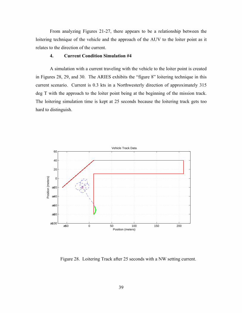
A simulation with a current traveling with the vehicle to the loiter point is created

in Figures 28, 29, and 30. The ARIES exhibits the “figure 8” loitering technique in this

current scenario. Current is 0.3 kts in a Northwesterly direction of approximately 315

deg T with the approach to the loiter point being at the beginning of the mission track.

The loitering simulation time is kept at 25 seconds because the loitering track gets too

hard to distinguish.

Figure 28. Loitering Track after 25 seconds with a NW setting current.

−50 0 50 100 150 200−100

−80

−60

−40

−20

0

20

40


Position (meters)

Pos

ition

(m

eter

s)

40

Figure 29. Loitering Track after 25 Seconds with a NW Setting Current.


0 5 10 15 20 25−25

−20

−15

−10

−5

0

5

10

15

20


Time (sec)

Rud

der

Ang

le (

Deg

)


−35 −30 −25 −20 −15 −10 −5 0 5 10 15−45

−40

−35

−30

−25

−20

−15

−10

−5

0Vehicle Track Data

Position (meters)

Pos

ition

(m

eter

s)

41

After analyzing the Figures 28-30, the shape of the loiter track at every turn with

this current condition is in a “figure 8”.


The current speed was increased to 1 kt for the same situations in the simulations

run earlier (Figures 15-30). Figures 31 and 32 below shows how the vehicle loitering

characteristics change with an increase in the current speed.

Figure 31. Loitering Track after 90 Seconds with a SE Setting Current.

−50 0 50 100 150 200−100

−80

−60

−40

−20

0

20

40


Position (meters)

Pos

ition

(m

eter

s)

42

Figure 32. Loitering Track after 90 seconds with a SE Setting Current.

Figures 31 and 32 show that the vehicle continues to exhibit irregularities in the

shape of the loitering track. The track above is a simulation of 90 second loitering time.

The boundedness of the loitering is also increased to a diameter of approximately 38

meters.


Next the direction at which the AUV proceeded to the loiter point was changed so

that the vehicle traveled into the current as it approached the loiter point. Figures 33 and

34 are the results.

−30 −20 −10 0 10 20−55

−50

−45

−40

−35

−30

−25

−20

−15

−10

−5

0Vehicle Track Data

Position (meters)

Pos

ition

(m

eter

s)

43


−50 0 50 100 150 200−100

−80

−60

−40

−20

0

20

40


Position (meters)

Pos

ition

(m

eter

s)

44


From Figures 33 and 34 again it is observed that when the vehicle proceeds to the

loiter point traveling against the current the loitering track shape is in a more predictable

manner. In this case, the shape becomes more semi-circular with a bounded diameter of

approximately 33 meters.


The current direction was changed to a Northeasterly direction and the vehicle

was again ordered to the loiter point by traveling directly into the onsetting current.

Figures 35 and 36 are the results.

−30 −20 −10 0 10 20−55

−50

−45

−40

−35

−30

−25

−20

−15

−10

−5

0Vehicle Track Data

Position (meters)

Pos

ition

(m

eter

s)

45

Figure 35. Loitering Track after 100 Seconds with a NE Setting Current.

−50 0 50 100 150 200−100

−80

−60

−40

−20

0

20

40


Position (meters)

Pos

ition

(m

eter

s)

46

Figure 36. Loitering Track after 100 Seconds with a NE Setting Current.

Figures 35 and 36 again show that there is a relationship with the approach track

to the loiter point and the current direction. The shape of the loitering track is semi-

circular in nature and bounded with a diameter of approximately 33 meters as in Figures

33 and 34.


The current direction was changed to a Northwesterly direction and the vehicle

proceeded with the current direction towards the loiter point. Figure 37 and 38 are the

results.

−30 −20 −10 0 10 20

−30

−20

−10

0

10

20

Vehicle Track Data

Position (meters)

Pos

ition

(m

eter

s)

47

Figure 37. Loitering Track after 100 Seconds with a NW Setting Current.

−50 0 50 100 150 200−100

−80

−60

−40

−20

0

20

40


Position (meters)

Pos

ition

(m

eter

s)

48

Figure 38. Loitering Track after 100 Seconds with NW Setting Current.

The characteristics of this track differ from the same approach that the AUV took

in Figures 28 through 30 is that this pattern is not dominated by “figure 8” tracks, but

rather an alternating semi-circular pattern. The pattern is still somewhat irregular in

nature and the track is now bounded by approximately 42 meters in diameter.

−50 −40 −30 −20 −10 0 10−35

−30

−25

−20

−15

−10

−5

0

5

10

15


Position (meters)

Pos

ition

(m

eter

s)

49

V. DISCUSSION OF RESULTS

A. RELATION BETWEEN APPROACH AND CURRENT DIRECTION

From the simulations and data collected, it was observed that the track the vehicle

traveled on during loiter is related to the position at where the vehicle was ordered to

proceed to the loiter point and the direction of the current. If ARIES proceeds to a loiter

point while traveling against the current, the shape of the loiter track is more predictable

and regular and the bounded area is minimized.

The reason for this relationship lies within the Cross Track Error Controller of

ARIES. When the vehicle is ordered to a loiter point, the heading directly to that position

becomes the track heading of the vehicle. As the vehicle passes over the loiter point, the

heading and steering controllers steer the vehicle in an attempt to regain the original track

heading, therefore, the AUV “circles” the point. As the vehicle circles the loiter point,

the current direction positions the AUV in such a manner that there is an ample distance

to proceed on the original track heading towards the loiter point and the process is

repeated. Figure 39 below is an illustration of what is being explained above. The

vehicle is on an original heading of 000 deg T and the current direction is 180 deg T. As

the vehicle passes over the loiter point, the controllers direct the vehicle is such a manner

so that it regains the 000 deg T track as it approaches the loiter point. The current

direction assists the controllers by setting the vehicle far enough away from the loiter

point that it can settle out on the 000 deg T leg.

50

Figure 39. Relation of Vehicle Approach and Current Direction.

B. LINE OF SIGHT GUIDANCE INSTABILITY

Since there is a relationship between the Cross Track Error Guidance and the

current direction, an analysis of using Line of Sight Guidance only during a loiter was

conducted. The vehicle does not need to get to the loiter station by a straight line using

Cross Track Error, it just needs to maintain a predictable and tight track pattern. A

simple simulation was run with the AUV using Line of Sight Guidance only during a

loiter and the results can be seen in Figure 40 below.

−40 −20 0 20 40 60−80

−70

−60

−50

−40

−30

−20

−10

0

10

Vehicle Track Data

Position (meters)

Pos

ition

(m

eter

s)

51

Figure 40. Line of Sight Guidance only during a loiter with no current.

Figure 40 shows that with Line of Sight Guidance only, the vehicle still has an

erratic and unpredictable track pattern. So the stability of the Line of Sight Guidance was

next analyzed thoroughly.

To analyze the stability of the Line of Sight Guidance the closed loop matrix of

the system was calculated. To calculate this the following was solved:

rBM

Y

rv

AM

Y

rv

δψψ

)()( 11 −− +

=

(24)

where,

−−

−=−

01004109.00507.008895.01492.0

)( 1AM

−40 −20 0 20 40 60−80

−70

−60

−50

−40

−30

−20

−10

0

10

20

Vehicle Track Data

Position (meters)

Pos

ition

(m

eter

s)

52

and

−=−

01650.0

1533.0)( 1BM

leaving equation (24) looking like:

r

Y

rv

UY

rv

δψψ

−

+

−−

−

=

001650.0

1533.0

0000010004109.00507.0008895.01492.0

where, U is the forward speed of the vehicle and rδ is incorporated from

equation (9).

comrkkrkvk ψψδ

4321−−−−= ;

where, Ydyd

com )( ψψ = and therefore leaving rδ as:

Ys

kkrkvkr )1(3321 +−−−= ψδ

where, 1k = 0 and 2k , 3k are taken from equation (9).

2

3

( 1.543)(2.5394)

( 1.5)

k

k η σφ

= −

= −

where, σ is solved from equation (8) and 0.1=η and 5.0=φ .

Now that rδ is in terms of

Y

rv

ψ, the A and B matrices can be combined in the

form:

53

[ ]

−=

Y

rv

BkA

Y

rv

ψψ

where, [ ]BkA − is the closed loop matrix, Ac, of the system. The eigenvalues of

Ac were found and plotted against the distance to the loiter point, s. Figure 41 below

shows the results.

Figure 41. Eigenvalues of LOS Guidance.

Figure 41 shows that the LOS Guidance system is stable farther away than close

in. The system goes unstable in this scenario approximately 3.9 meters from the loiter

point. Figure 42 is a closer look at the position at where the system goes unstable with an

Eigenvalue crossing the zero axis.

−10 0 10 20 30 40 50 60 70 80 90−12

−10

−8

−6

−4

−2

0

2

4

6Eigenvalues of LOS Guidance

Distance to Loiter Point (meters)

Eig

enva

lue

Eig#1Eig#2Eig#3Eig#4

54

Figure 42. Close In View where Eigenvalues of LOS Guidance Go Unstable.

Figures 41 and 42 explain the vehicle’s tendencies to be stable when it is a greater

distance away than when the vehicle is closer in. Under normal operations when the

vehicle is following a pre-programmed track with no loiter points, the stability of the

Line of Sight Guidance never becomes a problem because the watch radius around the

transition points or way points is usually set to approximately 10 meters. Therefore, the

AUV transitions to the next way point without the Line of Sight Guidance going

unstable. But when a loiter point is introduced into the program, the vehicle generally

cannot maintain a steady and predictable shape, but rather a random, unpredictable track

due to the instability of the Line of Sight Guidance.

0 1 2 3 4 5 6 7 8−1.5

−1

−0.5

0

0.5Eigenvalues of LOS Guidance

Distance to Loiter Point (meters)

Eig

enva

lue

Eig#1Eig#2Eig#3Eig#4

55

VI. STABILITY ANALYSIS

A. LIAPUNOV STABILITY/INSTABILITY THEOREMS

To investigate the instability of the Line of Sight Guidance even further, the

theorems of Liapunov were employed. Stability in the sense of the theories from

Liapunov is concerned with the behavior of a system in the vicinity of an equilibrium

state. Liapunov stated that if there exists a positive-definite function V(x) that is never

increasing, the origin is stable [8]. In this case, the origin is the loiter point.

In mathematical terms, the Liapunov Stability Theorem states if there exists a

continuously differentiable function V(x) such that:

1. V(0) = 0

2. V(x) > 0 for all x ≠ 0

3. ∑=

≤∂∂=′

∂∂=

n

ii

i

xfxVxf

xV

dtdV

10)()()( for all x

then the origin of the time-invariant system

)(xfx =

is stable.

Liapunov’s Instability Theorem states that if there exists a positive-definite

function V(x) whose derivative V (x) is non-negative in a region containing the origin,

then the origin is unstable.

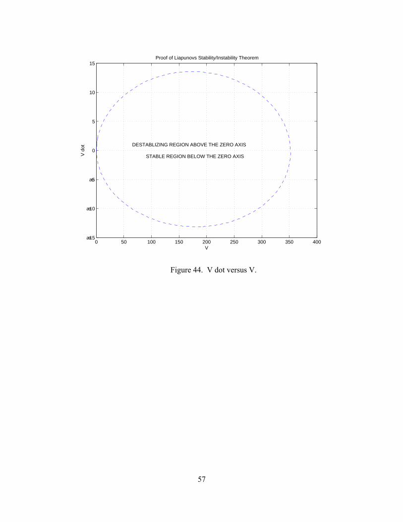
Applying this theory, a MATLAB program was created to compare the

Liapunov’s Stability/Instability Theorems to the loitering motions of the ARIES where a

Liapunov function was chosen and V versus V was plotted.

The program has the vehicle starting at a point very close to the origin, which is

the loitering station and the Liapunov function is 2 2( 10) ( 10)V x y= − + − . There are no

current conditions and Line of Sight Guidance is only used. Figures 43 and 44 below

56

provide proof through Liapunov’s Stability and Instability Theorems that the AUV’s Line

of Sight Guidance becomes unstable when it gets close to the origin (loiter point).

Figure 43. Vehicle Track Data of ARIES.

Figure 43 starts the AUV very close to its loiter point and the vehicle begins a

series of right turns to attempt to reach its programmed way point or loiter point in this

case. Figure 44 below shows how the Line of Sight Guidance is stable as it begins to

track into the point at a greater distance away, but then goes unstable when it gets a few

meters from the point.

8 10 12 14 16 18 20 22 24 26 28−4

−2

0

2

4

6

8

10

12


Position (meters)

Pos

ition

(m

eter

s)

57

Figure 44. V dot versus V.

0 50 100 150 200 250 300 350 400−15

−10

−5

0

5

10

15Proof of Liapunovs Stability/Instability Theorem

V

V d

ot DESTABLIZING REGION ABOVE THE ZERO AXIS

STABLE REGION BELOW THE ZERO AXIS

58


59

VII. CONCLUSIONS AND RECOMMENDATIONS

Although the loitering track of the ARIES is not predictable in most cases, the

loitering track of the vehicle is a bounded region for all cases. If a situation arises where

ARIES is required to maintain a circular pattern on a point or loiter station with no

deviation in its track, then a series of way points constructed in a circular, octagon, or box

pattern can be constructed and the vehicle will follow these points. This technique has

been proven through experiments run with the vehicle in previous missions.

Shutting the vehicle off at a loiter point is not an option for the following reasons.

Ultimately the AUV will operate in potentially hostile waters. If the vehicle is shut off at

its loiter station, the AUV will automatically surface making itself susceptible to enemy

detection and ultimately compromising its mission. Also, since the AUV is surfaced it

will still be effected by current conditions and will not maintain position on the loiter

point.

ARIES is constructed to be equipped with lateral and vertical thrusters. A

hovering control law algorithm could be constructed that would utilize the thrusters in the

vehicle’s attempt to maintain station on one point. This would prove to be useful because

the instability of the Line of Sight Guidance would not come into play if such a control

law existed, however, more power would be consumed in the process.

60


61

APPENDIX A. MATLAB FILES FOR AUV LOITERING The MATLAB code associated and developed for loitering behavior is contained

on CD-ROM and is obtainable through request from Professor A.J. Healey. This

appendix contains the MATLAB script file for the ARIES AUV to loiter and continue on

original track if desired. Currents can be introduced if desired.

LoiterToTrackRun.m

62


63

APPENDIX B. MATLAB FILES FOR AUV LOITERING The MATLAB code associated and developed for loitering behavior is contained


appendix contains the MATLAB script file for a simple approach to loiter for the ARIES

AUV.

simpleloiter.m

64


65

APPENDIX C. MATLAB FILES FOR AUV LOITERING The MATLAB code associated and developed for loitering behavior is contained


appendix contains the MATLAB script file for a simple approach to loiter for the ARIES

AUV using Line of Sight Guidance only. The eigenvalues of the closed loop LOS

Guidance are plotted versus distance to the loiter point to show instability.

LOSinstability.m

66


67

APPENDIX D. MATLAB FILES FOR AUV LOITERING The MATLAB code associated and developed for loitering behavior is contained


appendix contains the MATLAB script file to show the relationship between Liapunov’s

Stability/Instability Theorem to LOS Guidance.

Reverseinstability.m

68


69

LIST OF REFERENCES [1] Marco, D.B., Healey, A.J., “Command, Control, and Navigation Experimental Results With the NPS Aries AUV”, IEEE Journal of Oceanic Engineering , v.26, n.4, Oct. 2001, pp.466-476. [2] Ashtech Products, G12 Sensor, http://ashtech.com/Pages/prodoem.htm. [3] L. R. LeBlanc, M. Singer, P. Beaujean, et. Al., “Improved Chirp FSK Modem for High Reliability Communications in Shallow Water”, Proceedings IEEE Oceans 2000, IEEE #00CH37158C, pp. 601-603, 2000. [4] Healey, A.J., Lienard, D., “Multivariable Sliding Mode Control for Autonomous Diving and Steering of Unmanned Underwater Vehicles”, IEEE Journal of Oceanic Engineering, v.18, n.3, July 1993, pp.1-13. [5] Genon, G., An, E.P., Smith, S.M., Healey, A.J., “Enhancement of the Inertial Navigation System for the Morpheous Autonomous Underwater Vehicles”, IEEE Journal of Oceanic Engineering, v.26, n.4, Oct. 2001, pp.548-560. [6] Healey, A.J., An, E.P., Marco, D.B., “On Line Compensation of Heading Sensor Bias for Low Cost AUV Navigation”, Proceedings of IEEE AUV ’98, Cambridge, Mass, Aug. 20-21, 1998. [7] Cassandras, C.G., 1993, “Discrete Event Systems, Modeling and Performance Analysis”, Irwin-Aksen , ISBN-0-256-11212-6. [8] Friedland, B., 1996, “Advanced Control System Design”, Prentice-Hall, ISBN-0-13-0140104.

70


71

INITIAL DISTRIBUTION LIST 1. Defense Technical Information Center

Ft. Belvoir, VA 22060-6218

2. Dudley Knox Library Naval Postgraduate School Monterey, CA

3. Mechanical Engineering Department Chairman, Code ME Naval Postgraduate School Monterey, CA

4. Naval/Mechanical Engineering Curriculum Code 34

Naval Postgraduate School Monterey, CA

5. Professor Anthony J. Healey, Code ME/HY

Department of Mechanical Engineering Naval Postgraduate School

Monterey, CA

6. Dr. Donald Brutzman, Code UW/Br Undersea Warfare Group Naval Postgraduate School

Monterey, CA

7. Dr. T. B. Curtin, Code 322OM Office of Naval Research Arlington, VA

8. Dr. T. Swean, Code 32OE

Office of Naval Research Arlington, VA

9. LT Douglas L. Williams

Strategic Systems Program Kings Bay, GA

10. LT Joe Keller

Naval Postgraduate School Monterey, CA

72

11. LT Lynn Fodrea Naval Postgraduate School Monterey, CA

auv thesis revision#1 with matlab - 123seminarsonly.com · 2013-01-05 · as autonomous underwater...

Documents