Automatic Statistical Forecastingof Univariate Time Series

Use in Supply Chain Management (SCM) and Comparison of

Three Implementations

Marcel Baumgartnermarcel.baumgartner@nestle.com

Outline

Demand Planning / Statistical Forecasting in the Food Industry

ForecastPRO

State-Space Model of Exponential Smoothing

SAP Advanced Planning and Optimization(APO)

Comparison / Conclusions

Make-to-Stock

The Food Industry uses the Make-to-Stock approach: due to industrial constraints, we need to manufacture our products in advance, and we cannot wait for the order of the customer.

Therefore, foreseeing future orders is paramount. Weneed to make sure that we have the

• right product,• at the right location,• at the right moment in time,• with the right amount.

Demand Planning ProcessAt Nestlé, this planning process is known as Consensus Demand Planning.

The outcome of this process is a quantity per product, location and week (short term) / months (mid-term, up to 18 months), agreed upon by Sales, Marketing, Supply Chain and Finance functions, within the context of:

• high number or products• high innovation/renovation rate• need to forecast customer orders, and not real consumer demand• promotion driven business (need to capture consequences of

internal trade and marketing activities)• many categories depend on weather situation

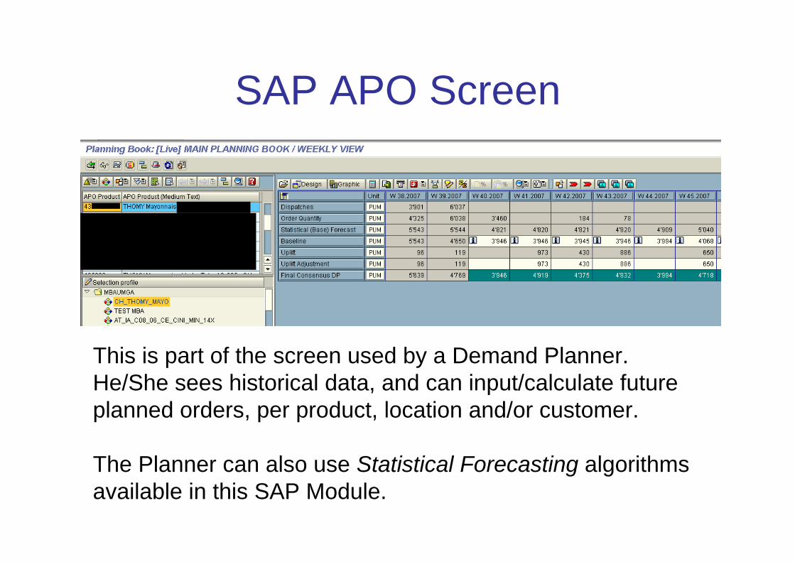
SAP APO Screen

This is part of the screen used by a Demand Planner. He/She sees historical data, and can input/calculate future planned orders, per product, location and/or customer.

The Planner can also use Statistical Forecasting algorithmsavailable in this SAP Module.

Examples of Time Series

Time (Months)

PUM

2500

0035

0000

4500

00

Jan 04 Jul 04 Jan 05 Jul 05 Jan 06 Jul 06 Jan 07

Time (Months)

PUM

2600

0032

0000

3800

00

Jan 04 Jul 04 Jan 05 Jul 05 Jan 06 Jul 06 Jan 07

Time (Months)

PUM

3000

050

000

7000

0

Jan 04 Jul 04 Jan 05 Jul 05 Jan 06 Jul 06 Jan 07

Time (Months)

PUM

5000

1000

015

000

2000

0

Jan 04 Jul 04 Jan 05 Jul 05 Jan 06 Jul 06 Jan 07

Examples of Time Series

Time (Months)

PUM

040

000

8000

014

0000

Jan 04 Jul 04 Jan 05 Jul 05 Jan 06 Jul 06 Jan 07

Time (Months)

PUM

5000

1500

025

000

Jan 04 Jul 04 Jan 05 Jul 05 Jan 06 Jul 06 Jan 07

Time (Months)

PUM

3000

040

000

5000

060

000

Jan 04 Jul 04 Jan 05 Jul 05 Jan 06 Jul 06 Jan 07

Time (Months)

PUM

8000

012

0000

1600

00

Jan 04 Jul 04 Jan 05 Jul 05 Jan 06 Jul 06 Jan 07

ForecastPRO

ForecastPRO is a renowed, best-of-breed statisticalforecasting software. It has a proven track record, notablyin the famous "M3 Forecasting Competition".

Its Expert Selection forecasting methods uses ExponentialSmoothing and ARIMA type algorithms. It can be run as a full black-box type method.

Advanced users can also choose themselves the family of method and the smoothing parameters.

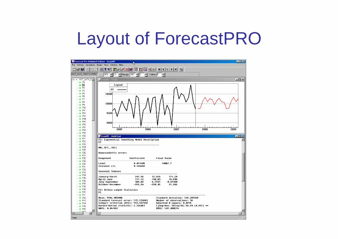
Layout of ForecastPRO

Add Screenshot from ForecastPRO

State Space Modelof Exponential Smoothing

This brand new approach is developed by Rob Hyndman, Monash University, Melbourne.

Rob Hyndman is co-author of "Business Forecasting: Methods and Applications" by Makridakis et al., and the lead author of a forthcoming book on ExponentialSmoothing.

Hyndman has developed a new framework for Exponential Smoothing based on State-Space Models. This allowed him to develop a much more robust approachto parameter fitting, and using Akaike type error measurements to estimate the "best" models.

His algorithm can also be run fully automatically. It is available in the package 'forecast' for R.

ETS() in R

SAP APO DP

SAP is one of the biggest business software provider. Nestlé supports its processes and best practices with SAP modules, in all kinds of areas, like Finance, Sales, Human Resources, Manufacturing, but also SupplyChain Management (SCM).

The main module for SCM is called APO (Advanced Planning and Optimization). A sub-module is related to Demand Planning. It containsstatistical forecasting algorithms, essentially based on ExponentialSmoothing and Linear Regression.

APO DP has a fully automated method as well, but its architecture isquite different compared to Hyndman's approach or the one fromForecastPRO.

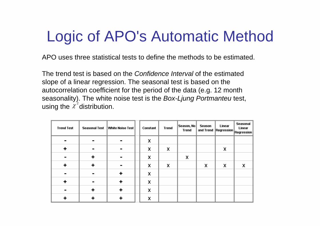
Logic of APO's Automatic Method

2χ

APO uses three statistical tests to define the methods to be estimated.

The trend test is based on the Confidence Interval of the estimatedslope of a linear regression. The seasonal test is based on the autocorrelation coefficient for the period of the data (e.g. 12 monthseasonality). The white noise test is the Box-Ljung Portmanteu test, using the distribution. 2χ

Overview of Methods

Best-of-breed statisticalforecasting software.

Internally developedexpert selection algorithm, without any detaileddocumentation.

Proven track record in forecast competitions.

Easy to use.

Extremely fast !

Brand new approach, "only" available in R. Based on a solid statistical foundation, using modern model selection criteria.

Algorithm documented in details.

Seems to compare well in the classic M3 competition.

Execution is slow, but easyto use and to parametrize.

Simple and straightforwardimplementation of exponential smoothing, withan automatic method basedon statistical tests.

Well documented, not as fastas ForecastPRO, but fasterthan the state-space model.

Has not been tested in forecasting competitions.

Well integrated in a business software for DemandPlanning.

Simulation Study

In order to study the quality of the forecasts of these threemethods, and also how differently they behave, we have simulated time series.

We vary 3 types of seasonality and 5 types of trend. This results in an experimental design of 15 combinations. For each combination, we generated 10 samples (differentrandom numbers).

Examples of Time Series

Time (Months)

Sal

es

5000

1000

015

000

2000

025

000

3000

0

2005 2006 2007 2008

Time (Months)

Sal

es

5000

1000

015

000

2000

025

000

3000

02005 2006 2007 2008

Time (Months)

Sal

es

5000

1000

015

000

2000

025

000

3000

0

2005 2006 2007 2008

Time (Months)

Sal

es

5000

1000

015

000

2000

025

000

3000

0

2005 2006 2007 2008

Time (Months)

Sal

es

5000

1000

015

000

2000

025

000

3000

0

2005 2006 2007 2008

Time (Months)

Sal

es

5000

1000

015

000

2000

025

000

3000

0

2005 2006 2007 2008

Time (Months)

Sal

es

5000

1000

015

000

2000

025

000

3000

0

2005 2006 2007 2008

Time (Months)

Sal

es

5000

1000

015

000

2000

025

000

3000

0

2005 2006 2007 2008

Time (Months)

Sal

es

5000

1000

015

000

2000

025

000

3000

0

2005 2006 2007 2008

Time (Months)

Sal

es

5000

1000

015

000

2000

025

000

3000

0

2005 2006 2007 2008

Time (Months)

Sal

es

5000

1000

015

000

2000

025

000

3000

0

2005 2006 2007 2008

Time (Months)

Sal

es

5000

1000

015

000

2000

025

000

3000

0

2005 2006 2007 2008

Time (Months)

Sal

es

5000

1000

015

000

2000

025

000

3000

0

2005 2006 2007 2008

Time (Months)

Sal

es

5000

1000

015

000

2000

025

000

3000

0

2005 2006 2007 2008

Time (Months)

Sal

es

5000

1000

015

000

2000

025

000

3000

0

2005 2006 2007 2008

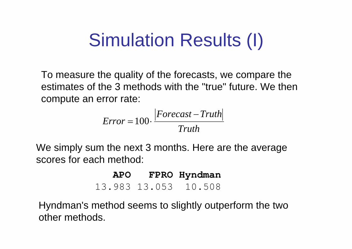
Simulation Results (I)

To measure the quality of the forecasts, we compare the estimates of the 3 methods with the "true" future. We thencompute an error rate:

TruthTruthForecast

Error−

⋅=100

We simply sum the next 3 months. Here are the averagescores for each method:

APO FPRO Hyndman13.983 13.053 10.508

Hyndman's method seems to slightly outperform the twoother methods.

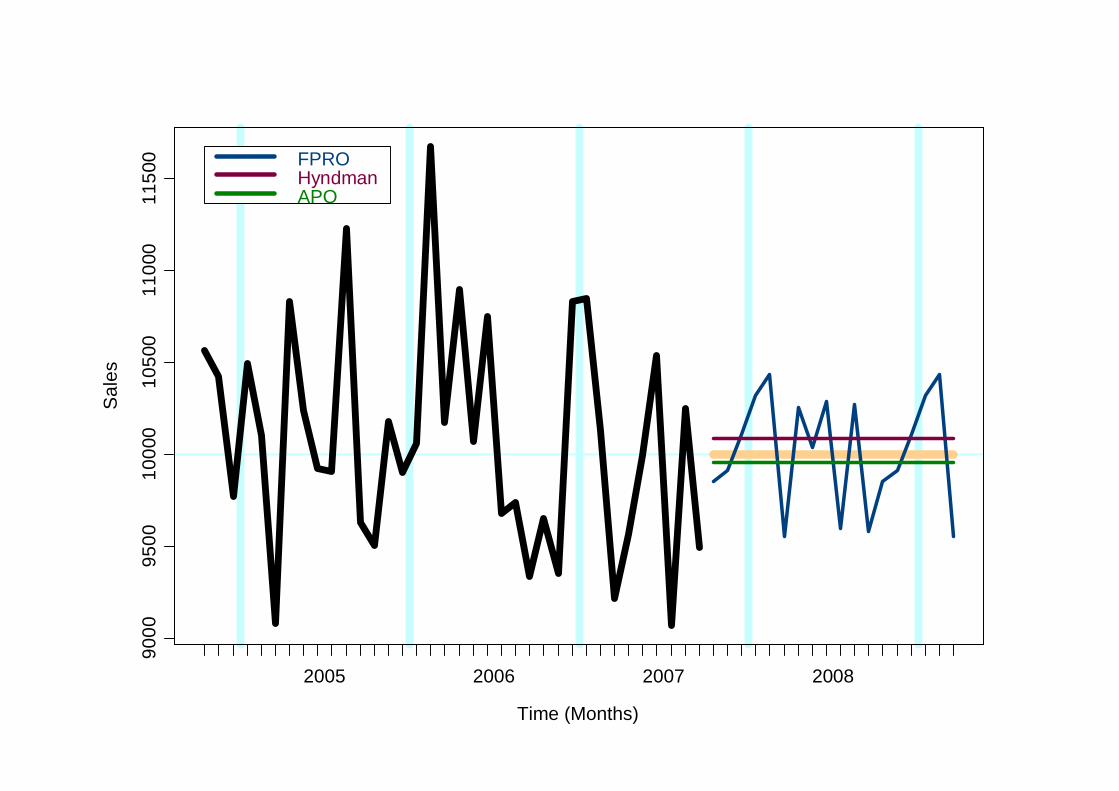
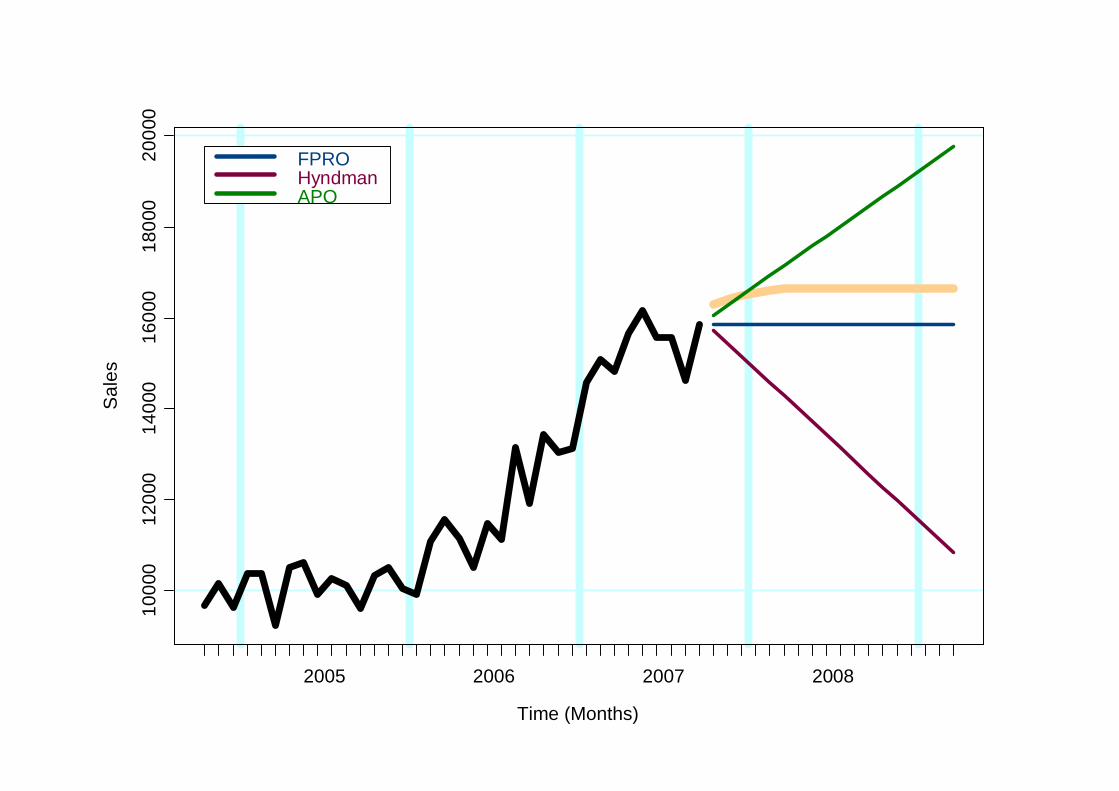
Simulation Results (II)

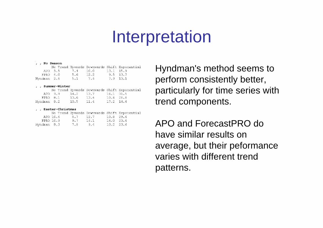
Interpretation

Hyndman's method seems to perform consistently better, particularly for time series withtrend components.

APO and ForecastPRO do have similar results on average, but their peformancevaries with different trend patterns.

Time (Months)

Sal

es

9000

9500

1000

010

500

1100

0

2005 2006 2007 2008

FPROHyndmanAPO

Time (Months)

Sal

es

9000

9500

1000

010

500

1100

011

500

2005 2006 2007 2008

FPROHyndmanAPO

Time (Months)

Sal

es

6000

8000

1000

012

000

1400

016

000

2005 2006 2007 2008

FPROHyndmanAPO

Time (Months)

Sal

es

9000

1000

011

000

1200

013

000

2005 2006 2007 2008

FPROHyndmanAPO

Time (Months)

Sal

es

9000

1000

011

000

1200

013

000

1400

015

000

2005 2006 2007 2008

FPROHyndmanAPO

Time (Months)

Sal

es

1000

012

000

1400

016

000

1800

020

000

2005 2006 2007 2008

FPROHyndmanAPO

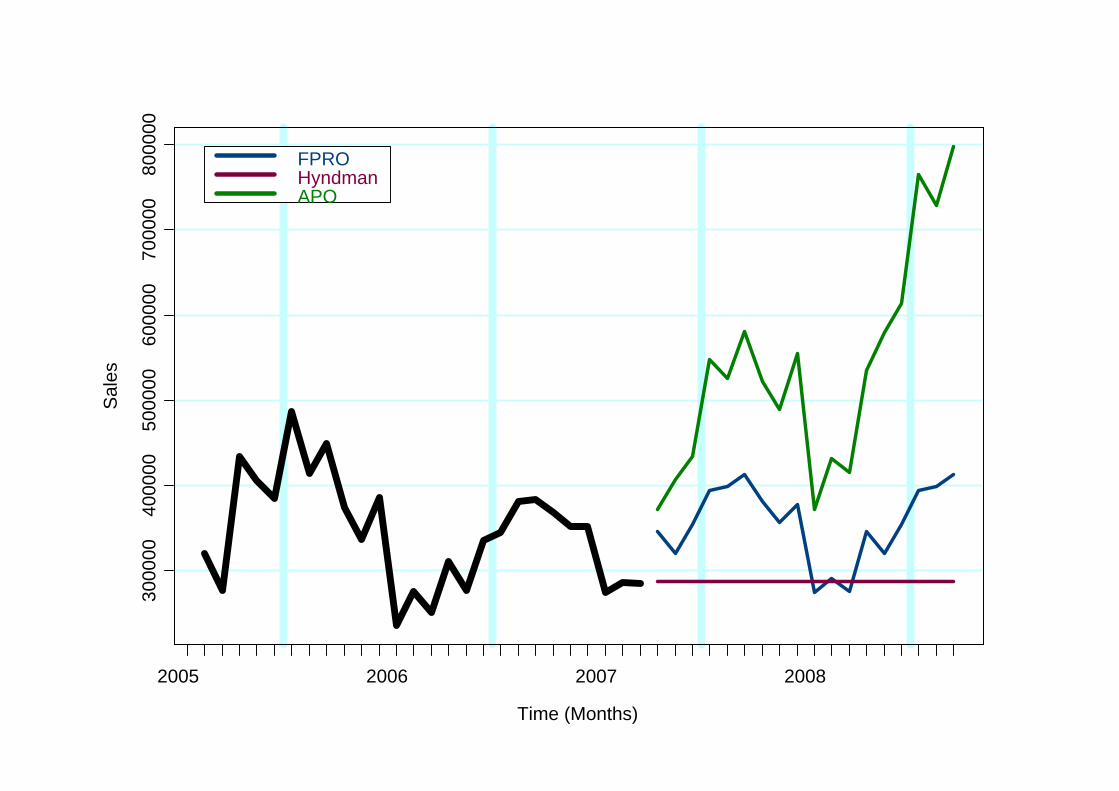
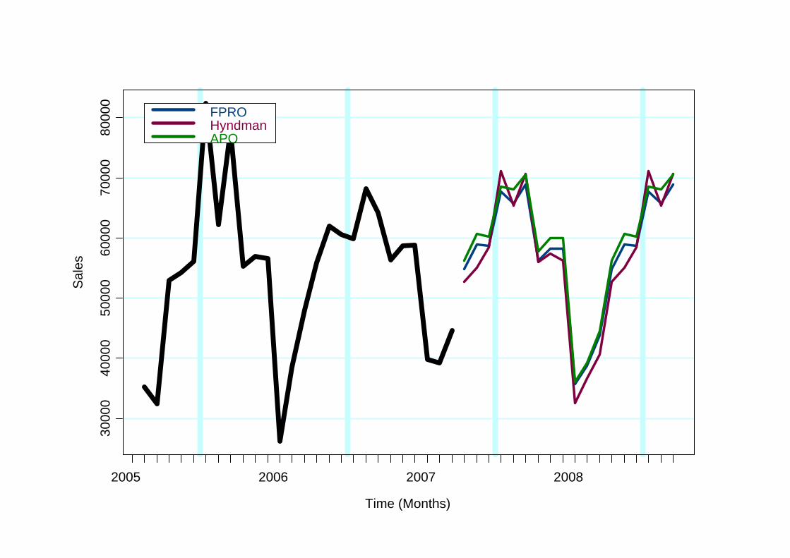
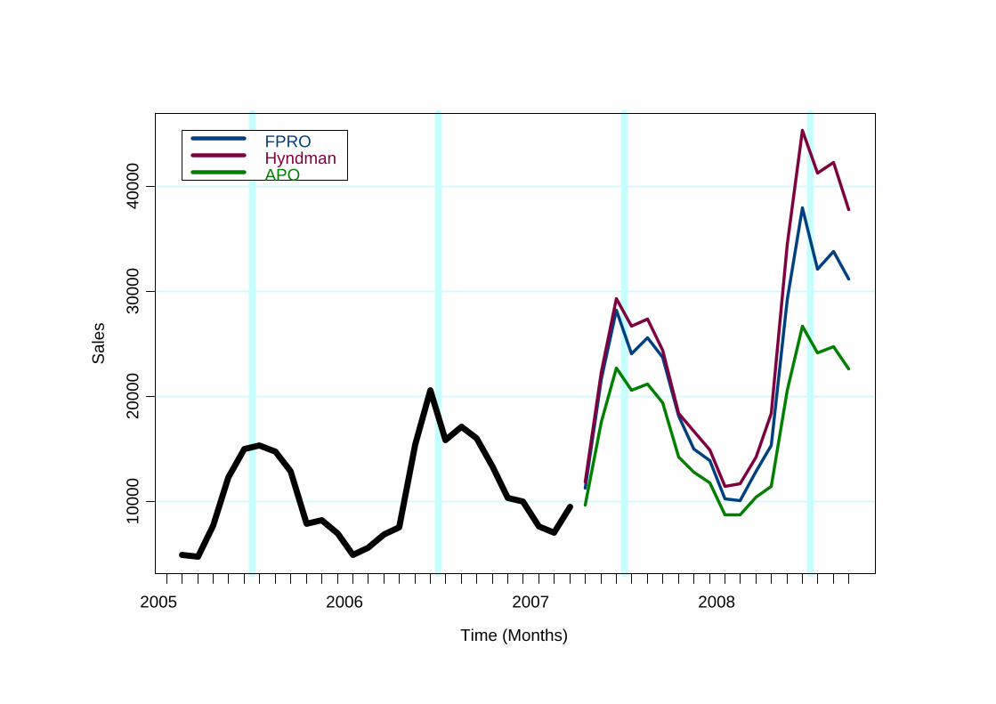
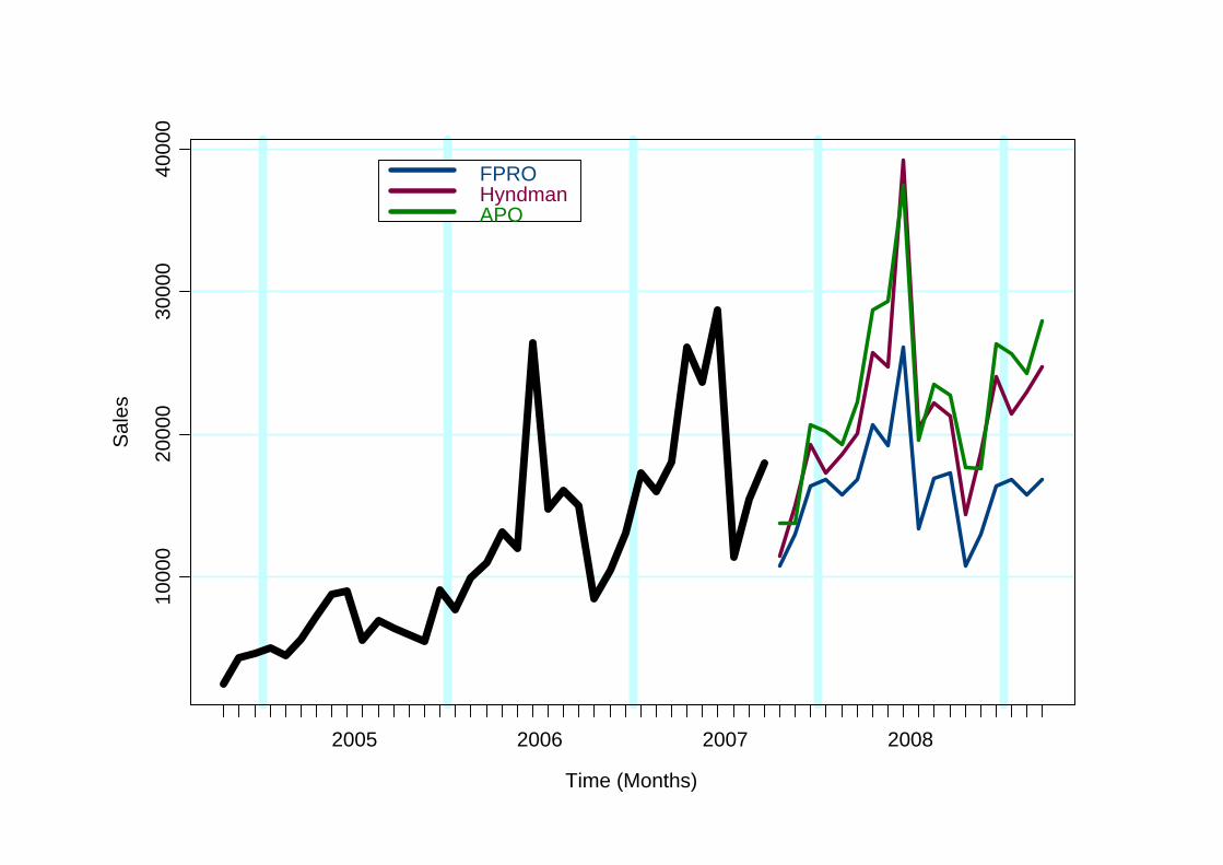
Real Data

We now show the results of the same forecastingmethods on the set of real time series presented earlier.

Time (Months)

Sal

es

3000

0040

0000

5000

0060

0000

7000

0080

0000

2005 2006 2007 2008

FPROHyndmanAPO

Time (Months)

Sal

es

2500

0030

0000

3500

0040

0000

4500

00

2005 2006 2007 2008

FPROHyndmanAPO

Time (Months)

Sal

es

3000

040

000

5000

060

000

7000

080

000

2005 2006 2007 2008

FPROHyndmanAPO

Time (Months)

Sal

es

1000

020

000

3000

040

000

2005 2006 2007 2008

FPROHyndmanAPO

Time (Months)

Sal

es

05*

10^5

10^6

1.5*

10^6

2*10

^62.

5*10

^6

2005 2006 2007 2008

FPROHyndmanAPO

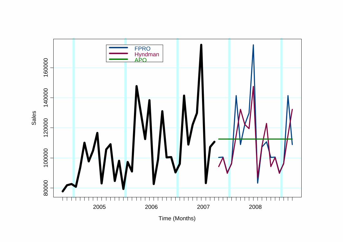
Here, Hyndman's method explodes !!!

Exponential Smoothing can sometimes generatequite crazy results.

We change the scale ...

Time (Months)

Sal

es

020

000

6000

010

0000

1400

00

2005 2006 2007 2008

FPROHyndmanAPO

Time (Months)

Sal

es

1000

020

000

3000

040

000

2005 2006 2007 2008

FPROHyndmanAPO

Time (Months)

Sal

es

3000

040

000

5000

060

000

7000

0

2005 2006 2007 2008

FPROHyndmanAPO

Time (Months)

Sal

es

8000

010

0000

1200

0014

0000

1600

00

2005 2006 2007 2008

FPROHyndmanAPO

ConclusionsThe different methods behave in a fairly similar way, and withgood results for the simulated data.

The more simplistic algorithm of APO also compares favorably with the more advanced approach of ForecastPROand with Hyndman's method, which has a more solidstatistical foundation. For noisy time series, more simple approaches sometimes work even better.

We can thus continue to improve and promote the use of the automatic forecasting method in APO, and follow-up the nextdevelopments in the area of state-space models for exponential smoothing.