Automatic Robot Calibration for the NAO

Tobias Kastner1, Thomas Rofer2, and Tim Laue1

1 Universitat Bremen, Fachbereich 3 – Mathematik und Informatik,Postfach 330 440, 28334 Bremen, Germany

E-Mail: {dyeah,tlaue}@informatik.uni-bremen.de2 Deutsches Forschungszentrum fur Kunstliche Intelligenz,

Cyber-Physical Systems, Enrique-Schmidt-Str. 5, 28359 Bremen, GermanyE-Mail: thomas.roefer@dfki.de

Abstract. In this paper, we present an automatic approach for the kine-matic calibration of the humanoid robot NAO. The kinematic calibra-tion has a deep impact on the performance of a robot playing soccer,which is walking and kicking, and therefore it is a crucial step prior toa match. So far, the existing calibration methods are time-consumingand error-prone, since they rely on the assistance of humans. The auto-matic calibration procedure instead consists of a self-acting measurementphase, in which two checkerboards, that are attached to the robot’s feet,are visually observed by a camera under several different kinematic con-figurations, and a final optimization phase, in which the calibration isformulated as a non-linear least squares problem, that is finally solvedutilizing the Levenberg-Marquardt algorithm.

1 Introduction

Calibration is the process of determining the relevant parameters of a roboticsystem by comparing the prediction of the system’s mathematical model withthe measurement of a known feature, which is considered as the standard. Ifthe difference between the prediction and the measurement exceeds a certaintolerance, it is inevitable to compensate for this mismatch to allow the robot tooperate as desired. The automatic calibration method presented in this paperis customized for the humanoid robot NAO [4] from Aldebaran Robotics. TheNAO has 21 degrees of freedom and is equipped with two cameras. The imagesare taken at a frequency of 30 Hz by each camera while other sensor data (suchas joint angle measurements) are updated at 100 Hz. The operating system isan embedded Linux that is powered by the Intel-Atom processor at 1.6 GHz.Since 2008, the NAO is the official platform of the RoboCup Standard PlatformLeague (SPL). To play soccer, a NAO has to be able to walk fast and to scoregoals. The overall performance of these two essential tasks strongly depends onprior precise calibration, which, so far, is a manual procedure that requires theassistance of human users. It is time-consuming and error-prone, since the errorsin the kinematics are estimated by eye and hand. These errors arise from theimprecise assembly of the robot itself and damage and wearout of the motors

during its operation. Consequently, it is often necessary to recalibrate a NAOafter a match. The goal of the automatic calibration that is presented in thispaper is to reduce the workload of human users, while providing comparableappropriate calibration parameters.

Markowsky [8] developed a method to calibrate the NAO’s leg kinematicsby using a hill climbing algorithm and a cost function that computes the dis-tribution of the current and weight loads of the two legs. The assumption wasthat the NAO is calibrated if the loads of each leg are similar. Due to poorsensor readings, this method turned out to be inapplicable. This paper is ratherinspired by the works of Birbach et al. [2], Pradeep et al. [11], and Nickels [10].These methods are based on the hand-eye calibration, which is explained byStrobl et al. [13]. The goal of these calibration procedures is to find the poses ofthe cameras in the robot’s head as well as the joint offsets that affect the properpositioning of the robot’s end effectors. The robot’s end effectors are driven topre-recorded positions and markers attached to these end effectors are visuallydetected by the robot’s cameras. Each position of the marker’s features in pixelcoordinates, as well as the respective joint angle measurements of the kinematicsare gathered and finally used to minimize the deviation between the actual visualmeasurements and the predicted ones based on the mathematical model of therobot, i. e. forward kinematics and extrinsic and intrinsic camera parameters.

In this paper, the NAO is calibrated by moving two checkerboards, whichare attached to the robot’s feet, in front of the lower camera of the NAO’s head.Similar to the related work presented, the image position of each vertex (point ofcontact of two isochromatic tiles) on the checkerboard is measured together withthe current joint angles. To formulate the calibration as a problem of non-linearleast squares, the forward kinematics of the NAO are computed with homoge-neous coordinate transformation and the projection function of the cameras isdescribed as a pinhole camera model. Using an a-priori intrinsic camera cali-bration and the Levenberg-Marquardt algorithm, the 21 parameters involved (12joint offsets, 3 camera rotation errors and 6 correction parameters for impre-cisely mounted checkerboards) are estimated by minimizing the sum of squaredresiduals of each measured vertex in pixels and the projection of the correspond-ing vertex from robot-relative coordinates to 2D image points, utilizing the jointangles measured.

The remainder of this paper is structured as follows: in the next section, theproperties of the checkerboard and foot-assembly as well as the formulation ofthe calibration as a problem of non-linear least squares are discussed. Section 3presents the results achieved, followed by Section 4, which concludes the paperand gives an outlook on possible future work and improvements to the calibrationprocedure presented.

2 Automatic Robot Calibration

First of all, the properties of the checkerboard sandals are discussed, followed bysome implementation details and the definition of the calibration as a non-linearleast squares problem.

2.1 Checkerboard Sandals

The checkerboard pattern with 35 tiles (7 columns and 5 rows) is printed on acustomized aluminum composite panel (see Fig. 1b) with a square size of 2.5 cm.Each board is mounted with four pins that exactly fit into the recesses locatedat the force-sensing resistors (FSR) on the bottom of the NAO’s feet (soles) anda further fixture with a hook and loop fastener tape. Since the positions of theFSRs (see Fig. 1a) are known relative to the projection of the ankle joint onthe sole, the positions of all 24 checkerboard vertices can be computed easily,considering that the center of the checkerboard is situated 17 cm away fromthe joint projection mentioned. These positions are used to predict the imagecoordinates of each vertex using the mathematical model of the NAO that stillhas to be defined.

2.2 Implementation

The calibration is implemented using the C++ framework [12] for modular de-velopment of robot control programs, published by the SPL team B-Human. Inthe context of this paper, a motion control engine, a checkerboard recognizer, anoptimization algorithm, and a calibration control module were developed. Anymore in-depth information on those software components can be found in thecorresponding thesis [5].

As proposed by Wiest [15] and Elatta et al. [3], the calibration is subdividedinto four phases modeling, measurement, identification, and compensation.

Modeling. The conversion from world to image coordinates is modeled withthe pinhole-camera model P :

P (x, y, z) = OC − (y, z)T flx. (1)

The optical center OC and the focal length fl were determined in a prior intrinsiccamera calibration, as proposed by Zhang [16].

The camera-relative world coordinates x, y, and z are computed using a mea-sured set of joint angles q, the forward kinematics TOLS(q), the transformationfrom the ankle joint to the left sole, and the positions of the checkerboard ver-tices computed relative to the feet pLSα. The functions Rotx, Roty, and Rotz areused to rotate a pose (position and rotation) around the respective axis, namedin the suffix. Likewise, the functions Transx, Transy, and Transz translate apose along the respective axis. In Fig. 2, the kinematic tree of the NAO is shown.

7.025 cm

2.99 cm 2.31 cm

0.8 cm2.965 cm

2.99 cm

(a)

17 cm

2.5 cm

2.5 cm

FSR

foot joint

(b)

Fig. 1. The positions of the FSRs on the sole (a). The checkerboard sandal with somedimension information (b).

Each joint angle qi is composed from the actual measured angle θi and theaffecting offset αi:

qi = θi + αi, i ∈{LHipY awPitch, LHipRoll, LHipP itch, (2)

LKneePitch, LAnkleP itch, LAnkleRoll,

RHipY awPitch, RHipRoll, RHipP itch,

RKneeP itch, RAnkleP itch, RAnkleRoll}.

Each element i stands for a servo motor that is able to measure its current anglewith a precision of 0.1◦ (the same precision applies to commanded angles). Theposition of each motor is visualized in Fig. 2.

The robot-relative pose of the lower camera is computed with TOC (homoge-neous transformation from the robot origin to the camera):

TOC (q, α) = TOC (q) ·Roty(αCamPitch) ·Rotx(αCamRoll) ·Rotz(αCamY aw). (3)

It is assumed that the actual camera pose TOC (q) is affected by three rotationaloffsets αCamPitch, αCamRoll, and αCamY aw.

HeadYaw

HeadPitch

LHipYawPitchRHipYawPitch

RHipRoll LHipRoll

RHipPitch LHipPitch

RKneePitch LKneePitch

RAnklePitch LAnklePitch

RAnkleRoll LAnkleRoll

left soleleft soleright soleright sole

lower cameralower camera

origin

CameraPitch

T LSOT RS

O

T CO

zz

yy

xx

Fig. 2. The kinematic tree of the NAO. The origin is located between the two hipmotors. The CameraPitch is a fixed assembly angle, taken from the official NAO doc-umentation. Any other motor angles are modifiable.

With the information on the checkerboard given in section 2.1, the coordi-nates of all vertices pLS , relative to the soles, can be computed.

pLSα = Rotz(αLRotZ) · Transx(αLTransX) · Transy(αLTransY ) · pLS . (4)

Since the pins on the boards are glued, it is possible that the assembly on thesoles is imprecise. In addition to the joint and camera correction offsets, threefurther parameters for each board are considered. It is assumed that the boardshave a rotational offset αLRotZ around the z-axis and a translational error in xand y direction (αLTransX and αLTransY ).

The final model is defined with proj(pLS , θ, α):

proj(pLS , θ, α) = P (TOC (q, α)−1 · TOLS(q) · pLSα). (5)

A given sole-relative vertex coordinate is transformed into origin coordinates,which gets further converted into camera-relative coordinates and is finally pro-jected onto the NAO’s camera plane, resulting in a prediction, where a vertexshould be located in the image, considering the current joint data and the cali-bration parameters.

The definitions given above are for the left leg kinematics. The missing pro-jection function for the right leg is computed analogously, using the right leg’sjoint data and the vertex positions from the right checkerboard. Also, only theleg’s kinematics are adjusted, since, so far, there are no actions that requireprecisely calibrated arms.

Table 1. Listing of all identified parameters. A type of ∆◦ indicates a rotational offsetand a ∆mm a translational offset.

Parameter Type Parameter Type Parameter Type

αCamY aw ∆◦ αCamPitch ∆◦ αCamRoll ∆◦

αLHipY awPitch ∆◦ αLHipRoll ∆◦ αLHipPitch ∆◦

αLKneePitch ∆◦ αLAnklePitch ∆◦ αLAnkleRoll ∆◦

αRHipY awPitch ∆◦ αRHipRoll ∆◦ αRHipPitch ∆◦

αRKneePitch ∆◦ αRAnklePitch ∆◦ αRAnkleRoll ∆◦

αLRotZ ∆◦ αLTransX ∆mm αLTransY ∆mm

αRRotZ ∆◦ αRTransX ∆mm αRTransY ∆mm

Altogether, the vertex-projection model is affected by 21 parameters (seeTab. 1), that need to be adjusted. The crucial parameters are the three rota-tional camera corrections and the twelve leg joint offsets. Note that this set ofparameters is the same that is used in the manual calibration procedures.

Measurement. The target measurements are the 2D image coordinates of thecheckerboard vertices. The localization of these vertices is accomplished with acombination of the vertex detection algorithm of Bennet et al. [1], the chessboardextraction method of Wang et al. [14], and the sub-pixel refinement implementedby Birbach et al. [2]. These methods operate on the grey-scale images of the lowercamera with VGA resolution.

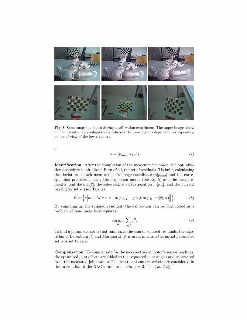
To assure that the calibration can be performed secure and unsupervised, theNAO is lying on its back, while driving to 24 different leg stances (for both legs).For each configuration, the checkerboard is observed incorporating three differenthead postures. The configurations are chosen heuristically, considering that thecheckerboard is fully visible, while having different rotations and distances to thecamera. Note that the checkerboard vertices are only detected after the robotreached its desired stance, since there is a lag between the arrival of a new cameraimage and the sensor readings. The complete self-acting measurement phase isvisualized in Fig. 3.

For each vertex observed, a new measurement m is collected and added to aset M :

M ={m0,m1, . . . ,mn

}. (6)

A measurement is a triple, consisting of the image position pimg, the correspond-ing sole-relative 3D coordinate of the vertex pcb, and the measured joint angles

0 1 2 3 4 5

6 7 8 9 10 11

12 13 14 15 16 17

18 19 20 21 22 23

0 1 2 3 4 56 7 8 9 10 1112 13 14 15 16 17

18 19 20 21 22 23

01 2

34

567

89

101112

1314

1516

1718

1920

2122

23

Fig. 3. Some snapshots taken during a calibration experiment. The upper images showdifferent joint angle configurations, whereas the lower figures depict the correspondingpoints of view of the lower camera.

θ:m = (pimg, pcb, θ). (7)

Identification. After the completion of the measurement phase, the optimiza-tion procedure is initialized. First of all, the set of residuals R is built, calculatingthe deviation of each measurement’s image coordinate m[pimg] and the corre-sponding prediction, using the projection model (see Eq. 5) and the measure-ment’s joint data m[θ], the sole-relative vertex position m[pcb], and the currentparameter set α (see Tab. 1):

R ={r∣∣∣m ∈M ∧ r =

∥∥∥m[pimg]− proj(m[pcb],m[θ], α)∥∥∥}. (8)

By summing up the squared residuals, the calibration can be formulated as aproblem of non-linear least squares:

arg minα

∑r∈R

r2. (9)

To find a parameter set α that minimizes the sum of squared residuals, the algo-rithm of Levenberg [7] and Marquardt [9] is used, in which the initial parameterset α is set to zero.

Compensation. To compensate for the incorrect servo motor’s sensor readings,the optimized joint offsets are added to the requested joint angles and subtractedfrom the measured joint values. The rotational camera offsets are considered inthe calculation of the NAO’s camera matrix (see Rofer et al. [12]).

3 Results

This section outlines the results of the automatic robot calibration, beginningwith a simulated calibration and a concluding calibration experiment executedwith a real NAO.

3.1 Simulation

With the help of SimRobot [6], the calibration’s feasibility was tested. A simu-lated NAO was modeled with random erroneous joint offsets and with imprecisecheckerboard assembly. As Fig. 4a and Fig. 4b imply, all errors were correctlycompensated. Since the errors for each leg chain are different, the residual dis-tribution for the left and right leg exhibit different appearances (see Fig. 4a).Apparent from Fig. 4b, the adjusted parameters create a normal distributionwith zero mean and a standard deviation of 0.0486 pixels in x and 0.0403 pixelsin y direction.

3.2 NAO

On a real NAO, three consecutive automatic calibrations were executed3. Be-forehand, an intrinsic camera calibration was done, resulting in a focal lengthof 562.5 pixels and an optical center of (324, 189)

Tpixels. The resulting pa-

rameters, as well as further information, such as the calibration duration, areshown in Tab. 2. One calibration round took 590 seconds on average and theLevenberg-Marquardt algorithm converged after 41 iterations on average. Theroot mean squared error was reduced to roughly three pixels in x and two anda half pixels in y direction. It is noticeable, regarding the optimized parameters,that the left leg’s pitch motor deviations are rather big, with a value of 0.5421◦

at a max. This implies that there are several different configurations that mini-mize the sum of squared residuals. In contrast, the right leg’s parameters have amaximal deviation of 0.2413◦. The vast majority of the parameters were similarafter the three calibration runs, in particular the three camera rotation offsets.The checkerboard assembly correction parameters are adequately small.

It is obvious that the resulting parameters are not a perfect solution to theminimization problem, since there are many residuals bigger than the threefoldstandard deviation (see Fig. 4d). Unlike the depiction of Fig. 5, where (a) isshowing the projection of the checkerboard before and (b) after a calibration,there are countless kinematic configurations resulting in an imprecise projection.A standard test for a good calibration of the camera’s pose is the projection ofthe modeled lines of an official SPL field back into the image from a knownposition on the field and comparing them with the lines that are actually seen.However, using the optimized parameters, this test showed unsatisfactory results.

3 The gathered data of the three experiments can be found as CSV files on:https://sibylle.informatik.uni-bremen.de/public/calibration/

-12

-8

-4

0

4

8

12

-12 -8 -4 0 4 8 12

resi

dual y in p

ixel

residual x in pixel

right legleft leg

(a)

-0.5

-0.4

-0.3

-0.2

-0.1

0

0.1

0.2

0.3

0.4

0.5

-0.5 -0.4 -0.3 -0.2 -0.1 0 0.1 0.2 0.3 0.4 0.5

resi

dual y in p

ixel

residual x in pixel

right legleft leg

(b)

-75

-60

-45

-30

-15

0

15

30

45

60

75

-75 -60 -45 -30 -15 0 15 30 45 60 75

resi

dual y in p

ixel

residual x in pixel

right legleft leg

(c)

-18

-15

-12

-9

-6

-3

0

3

6

9

12

15

18

-18 -15 -12 -9 -6 -3 0 3 6 9 12 15 18

resi

dual y in p

ixel

residual x in pixel

right legleft leg

(d)

Fig. 4. Residual distribution of a simulated calibration (a) without and (b) with opti-mized parameters. The lower figures visualize the residual distribution of the first outof three calibration experiments on a real NAO: distribution (c) without and (d) withadjusted parameters. Note that the axes have different ranges.

The most probable cause is backlash that has a different impact on a robot lyingon its back than on a standing robot.

Using the parameters of the third calibration run, the NAO was able to playsoccer for the duration of a half (10 minutes), while falling down 6 times. Withouta calibration, the NAO fell down 11 times in the same amount of time. Furtherexperiments with four other NAOs exhibited a similar result: a calibration nevernegatively influenced the performance of a NAO playing soccer. In one case,a robot, that was initially not able to walk half a meter, was able to play acomplete half (still being very shaky and unstable).

(a) (b)

Fig. 5. The checkerboard projection without calibration (a). The resulting projectionwith optimized parameters α (b).

4 Conclusion

In this paper, we presented a method to define an automatic robot calibration asa problem of non-linear least squares, customized for the humanoid robot NAO.The NAO was modeled with the help of homogeneous coordinate transformationand the pinhole camera model. The resulting least squares problem was solvedwith the Levenberg-Marquardt algorithm.

The simulated calibrations resulted in perfect estimates for the compensa-tion of the identified errors and therefore prove the plausibility of the presentedapproach. Performing the calibration with real NAOs turned out to be less sat-isfying. Apart from the fast overall operation time with roughly 10 minutes, thedeviations of some parameters after consecutive calibrations vary strongly, theprojection of field lines was rather imprecise, and there are many joint configura-tions that resulted in an insufficient re-projection of the checkerboard. However,the kinematic parameters can be used as a better initial guess for a manualcalibration.

We think that the extension of the projection model with non-geometricerrors, such as joint elasticities, could improve the results. Birbach et al. [2] andWiest [15] modeled elasticities with a spring, using the torques that affect eachmotor. Since the NAO lacks of torque sensors, only static torques can be used.It is also conceivable that the lengths of the limbs may vary from the values inthe official NAO documentation. The most difficult unregarded errors are thosethat result from backlash, which, according to Gouaillier et al. [4], might havea range of ±5◦. In addition, the offsets of the two head joints might also impairthe calibration result, because they are not adjusted during the optimization,since they might have a linear dependency to the camera rotation offsets.

The improvement of this calibration approach will be further investigated byconsidering the possible problems mentioned.

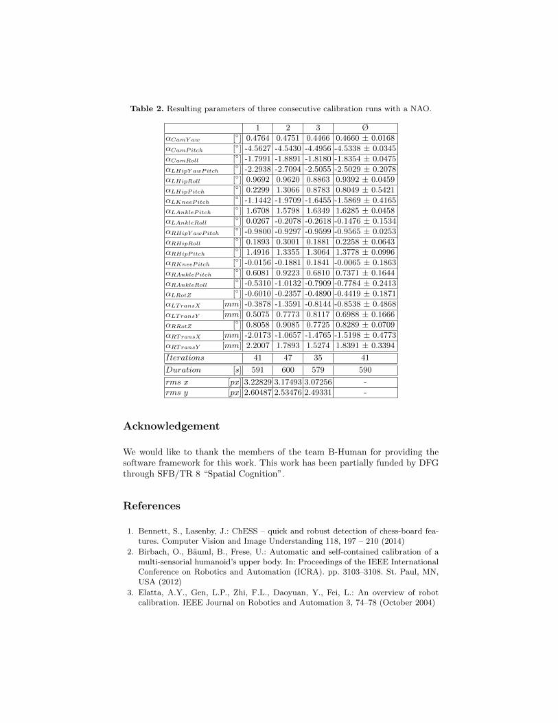
Table 2. Resulting parameters of three consecutive calibration runs with a NAO.

1 2 3 Ø

αCamY aw [◦] 0.4764 0.4751 0.4466 0.4660 ± 0.0168

αCamPitch [◦] -4.5627 -4.5430 -4.4956 -4.5338 ± 0.0345

αCamRoll [◦] -1.7991 -1.8891 -1.8180 -1.8354 ± 0.0475

αLHipY awPitch [◦] -2.2938 -2.7094 -2.5055 -2.5029 ± 0.2078

αLHipRoll [◦] 0.9692 0.9620 0.8863 0.9392 ± 0.0459

αLHipPitch [◦] 0.2299 1.3066 0.8783 0.8049 ± 0.5421

αLKneePitch [◦] -1.1442 -1.9709 -1.6455 -1.5869 ± 0.4165

αLAnklePitch [◦] 1.6708 1.5798 1.6349 1.6285 ± 0.0458

αLAnkleRoll [◦] 0.0267 -0.2078 -0.2618 -0.1476 ± 0.1534

αRHipY awPitch [◦] -0.9800 -0.9297 -0.9599 -0.9565 ± 0.0253

αRHipRoll [◦] 0.1893 0.3001 0.1881 0.2258 ± 0.0643

αRHipPitch [◦] 1.4916 1.3355 1.3064 1.3778 ± 0.0996

αRKneePitch [◦] -0.0156 -0.1881 0.1841 -0.0065 ± 0.1863

αRAnklePitch [◦] 0.6081 0.9223 0.6810 0.7371 ± 0.1644

αRAnkleRoll [◦] -0.5310 -1.0132 -0.7909 -0.7784 ± 0.2413

αLRotZ [◦] -0.6010 -0.2357 -0.4890 -0.4419 ± 0.1871

αLTransX [mm] -0.3878 -1.3591 -0.8144 -0.8538 ± 0.4868

αLTransY [mm] 0.5075 0.7773 0.8117 0.6988 ± 0.1666

αRRotZ [◦] 0.8058 0.9085 0.7725 0.8289 ± 0.0709

αRTransX [mm] -2.0173 -1.0657 -1.4765 -1.5198 ± 0.4773

αRTransY [mm] 2.2007 1.7893 1.5274 1.8391 ± 0.3394

Iterations 41 47 35 41

Duration [s] 591 600 579 590

rms x [px] 3.22829 3.17493 3.07256 -

rms y [px] 2.60487 2.53476 2.49331 -

Acknowledgement

We would like to thank the members of the team B-Human for providing thesoftware framework for this work. This work has been partially funded by DFGthrough SFB/TR 8 “Spatial Cognition”.

References

1. Bennett, S., Lasenby, J.: ChESS – quick and robust detection of chess-board fea-tures. Computer Vision and Image Understanding 118, 197 – 210 (2014)

2. Birbach, O., Bauml, B., Frese, U.: Automatic and self-contained calibration of amulti-sensorial humanoid’s upper body. In: Proceedings of the IEEE InternationalConference on Robotics and Automation (ICRA). pp. 3103–3108. St. Paul, MN,USA (2012)

3. Elatta, A.Y., Gen, L.P., Zhi, F.L., Daoyuan, Y., Fei, L.: An overview of robotcalibration. IEEE Journal on Robotics and Automation 3, 74–78 (October 2004)

4. Gouaillier, D., Hugel, V., Blazevic, P., Kilner, C., Monceaux, J., Lafourcade, P.,Marnier, B., Serre, J., Maisonnier, B.: The NAO humanoid: a combination of per-formance and affordability. CoRR abs/0807.3223 (2008)

5. Kastner, T.: Automatische Roboterkalibrierung fur den humanoiden RoboterNAO. Diploma thesis, Universitat Bremen (2014)

6. Laue, T., Spiess, K., Rofer, T.: SimRobot – a general physical robot simulatorand its application in RoboCup. In: RoboCup 2005: Robot Soccer World Cup IX.Lecture Notes in Artificial Intelligence, vol. 4020, pp. 173–183. Springer (2006)

7. Levenberg, K.: A method for the solution of certain problems in least squares. TheQuarterly of Applied Mathematics 2, 164–168 (1944)

8. Markowsky, B.: Semiautomatische Kalibrierung von Naogelenken. Bachelor thesis,Universitat Bremen (2011)

9. Marquardt, D.W.: An algorithm for least-squares estimation of nonlinear parame-ters. SIAM Journal on Applied Mathematics 11(2), 431–441 (1963)

10. Nickels, K.M., Baker, K.: Hand-eye calibration for Robonaut. Tech. rep, NASASummer Faculty Fellowship Program Final Report, Johnson Space Center (2003)

11. Pradeep, V., Konolige, K., Berger, E.: Calibrating a multi-arm multi-sensor robot:A bundle adjustment approach. In: International Symposium on ExperimentalRobotics (ISER). New Delhi, India (12/2010 2010)

12. Rofer, T., Laue, T., Muller, J., Bartsch, M., Batram, M.J., Bockmann, A., Boschen,M., Kroker, M., Maaß, F., Munder, T., Steinbeck, M., Stolpmann, A., Taddiken,S., Tsogias, A., Wenk, F.: B-Human team report and code release 2013 (2013),only available online: http://www.b-human.de/downloads/publications/2013/

CodeRelease2013.pdf

13. Strobl, K.H., Hirzinger, G.: Optimal hand-eye calibration. In: Proceedings of the2006 IEEE/RSJ International Conference on Intelligent Robots and Systems (IROS2006). pp. 4647–4653. IEEE, Beijing, China (2006)

14. Wang, Z., Wu, W., Xu, X.: Auto-recognition and auto-location of the internalcorners of planar checkerboard image. In: International Conference on IntelligentComputing. pp. 473–479. Heifei, China (2005)

15. Wiest, U.: Kinematische Kalibrierung von Industrierobotern. Berichte aus der Au-tomatisierungstechnik, Shaker Verlag (2001)

16. Zhang, Z.: A flexible new technique for camera calibration. IEEE Transactions onPattern Analysis and Machine Intelligence 22, 1330–1334 (1998)