This is a repository copy of Automatic rationalization of yield-line patterns identified using discontinuity layout optimization.

White Rose Research Online URL for this paper:http://eprints.whiterose.ac.uk/94918/

Version: Accepted Version

Article:

He, L. and Gilbert, M. (Accepted: 2015) Automatic rationalization of yield-line patterns identified using discontinuity layout optimization. International Journal of Solids and Structures. ISSN 0020-7683

https://doi.org/10.1016/j.ijsolstr.2015.12.014

This is the peer reviewed version of the following article: He, Linwei, and Matthew Gilbert. "Automatic rationalization of yield-line patterns identified using discontinuity layout optimization." International Journal of Solids and Structures (2015)., which has been published in final form at https://dx.doi.org/10.1016/j.ijsolstr.2015.12.014. This article may be used for non-commercial purposes in accordance with Wiley Terms and Conditions for Self-Archiving (http://olabout.wiley.com/WileyCDA/Section/id-820227.html).

eprints@whiterose.ac.ukhttps://eprints.whiterose.ac.uk/

Reuse

Unless indicated otherwise, fulltext items are protected by copyright with all rights reserved. The copyright exception in section 29 of the Copyright, Designs and Patents Act 1988 allows the making of a single copy solely for the purpose of non-commercial research or private study within the limits of fair dealing. The publisher or other rights-holder may allow further reproduction and re-use of this version - refer to the White Rose Research Online record for this item. Where records identify the publisher as the copyright holder, users can verify any specific terms of use on the publisher’s website.

Takedown

If you consider content in White Rose Research Online to be in breach of UK law, please notify us by emailing eprints@whiterose.ac.uk including the URL of the record and the reason for the withdrawal request.

Accepted Manuscript

Automatic rationalization of yield-line patterns identified using

discontinuity layout optimization

Linwei He, Matthew Gilbert

PII: S0020-7683(15)00506-5

DOI: 10.1016/j.ijsolstr.2015.12.014

Reference: SAS 8995

To appear in: International Journal of Solids and Structures

Received date: 20 May 2015

Revised date: 16 November 2015

Accepted date: 13 December 2015

Please cite this article as: Linwei He, Matthew Gilbert, Automatic rationalization of yield-line patterns

identified using discontinuity layout optimization, International Journal of Solids and Structures (2015),

doi: 10.1016/j.ijsolstr.2015.12.014

This is a PDF file of an unedited manuscript that has been accepted for publication. As a service

to our customers we are providing this early version of the manuscript. The manuscript will undergo

copyediting, typesetting, and review of the resulting proof before it is published in its final form. Please

note that during the production process errors may be discovered which could affect the content, and

all legal disclaimers that apply to the journal pertain.

ACCEPTED MANUSCRIPT

ACCEPTED

MA

NU

SCRIP

T

Automatic rationalization of yield-line patterns identified

using discontinuity layout optimization

Linwei Hea, Matthew Gilberta,∗

aDepartment of Civil and Structural Engineering,University of Sheffield, Sir Frederick Mappin Building,

Mappin Street, Sheffield, S1 3JD, UK

Abstract

The well-known yield-line analysis procedure for slabs has recently been systematically

automated, enabling the critical yield-line pattern to be identified quickly and easily,

whatever the slab geometry. This has been achieved by using the discontinuity layout

optimization (DLO) procedure, which involves using optimization to identify the critical

layout of yield-line discontinuities interconnecting regularly spaced nodes distributed

across a slab. However, whilst highly accurate solutions can be obtained, the corre-

sponding yield-line patterns are often quite complex in form, especially when relatively

dense nodal grids are employed. Here a method of rationalizing the DLO-derived yield-

line patterns via a geometry optimization post-processing step is described. Geometry

optimization involves adjusting the positions of the nodes, thereby simultaneously sim-

plifying and improving the accuracy of the solution. The mathematical expressions

involved are derived analytically, and various practical issues are highlighted and ad-

dressed. Finally, an interior point optimizer is used to obtain rationalized solutions for

a variety of sample slab analysis problems, clearly demonstrating the efficacy of the

proposed rationalization technique.

Keywords: Discontinuity layout optimization, yield-line analysis, geometry

optimization

∗Corresponding author. Email: m.gilbert@sheffield.ac.uk

Preprint submitted to International Journal of Solids and Structures December 30, 2015

ACCEPTED MANUSCRIPT

ACCEPTED

MA

NU

SCRIP

T

1. Introduction

The yield-line method of analysis proposed by Johansen (1943) provides a powerful

means of computing the collapse load factor of a reinforced concrete slab. The method,

which provides upper bound solutions within the context of the formal theorems of plas-

ticity, requires a kinematically admissible failure mechanism to be prescribed, defined

by means of a yield-line pattern. The early focus was on slabs with relatively simple

geometries (e.g., Johansen 1943, 1968) because, at the time, systematic means of iden-

tifying the critical failure mechanism for irregularly shaped slabs were not available.

Subsequently Chan (1972) and Munro and Da Fonseca (1978) proposed a means of au-

tomatically identifying the critical yield-line pattern. This involved discretizing a slab

using rigid finite-elements, with the critical yield-line pattern then obtained automati-

cally via linear optimization. However, because yield-lines were restricted to forming

only at the edges of the finite-elements, the resulting yield-line patterns were signifi-

cantly influenced by the initial mesh topology. Attempting to address this issue, various

workers proposed the use of ‘geometry optimization’ to subsequently adjust the posi-

tions of selected nodes in a post-processing phase. For example, Johnson (1994, 1995)

proposed that this be achieved via the use of sequential linear programming. Other

workers to propose a similar approach included Thavalingam et al. (1999), who em-

ployed a conjugate gradient optimizer, and Ramsay and Johnson (1997, 1998), who

used a direct search solver. However, as indicated by Ramsay et al. (2015), the outcomes

will be affected by the initial mesh topology, and a poor initial solution will render any

subsequent geometry optimization phase largely ineffective. Another issue is the need

to manually identify yield-lines from the finite-element meshes; any misinterpretation

can reduce the efficacy of the geometry optimization phase. This has been described as

being ‘difficult’ (e.g., Johnson 1994, Thavalingam et al. 1999). As an alternative, plate

formulations in which deformations can take place within elements, rather than just at

element boundaries, have been proposed, with pioneering work in this field undertaken

by Hodge and Belytschko (1968) and Anderheggen and Knopfel (1972). However, with

2

ACCEPTED MANUSCRIPT

ACCEPTED

MA

NU

SCRIP

T

such formulations the yield-line pattern can be somewhat difficult to discern.

More recently, Jackson (2010) and Jackson and Middleton (2013) used a lower-

bound finite element solution to derive ‘yield-line indicators’, which could be used to

infer the likely general form of the critical yield line pattern. This then enabled a more

refined yield-line pattern to be identified via a geometry optimization step. The resulting

procedure allowed reasonable yield-line analysis solutions to be obtained for complex

slab problems. However, as the procedure involved a manual interpretation step, a truly

systematic means of automatically identifying the critical yield-line pattern remained to

be found.

Recently, this goal was achieved by Gilbert et al. (2014), who used discontinuity lay-

out optimization (DLO) to automate the process of identifying the most critical yield-

line pattern. Instead of discretizing the problem using elements arranged in a finite

element mesh, when using DLO the slab area is populated by nodes, and these are then

interconnected with a large set of potential yield-lines, which are free to cross-over one

another. A highly efficient optimization process is then used to find the critical subset

of yield-lines involved in the critical failure mechanism. An overview of the steps in-

volved in the DLO procedure is shown in Fig. 1. Improved solutions can be obtained by

using an increased number of nodes; the resulting greatly increased number of poten-

tial yield-lines can be handled efficiently using the adaptive solution scheme proposed

for truss layout optimization by Gilbert and Tyas 2003, and used for this application in

Gilbert et al. 2014. However, whilst highly accurate solutions can be obtained using the

DLO procedure, the corresponding yield-line patterns are often quite complex in form,

especially when relatively dense nodal grids are employed. In an attempt to address this,

a modified formulation was also proposed by Gilbert et al. (2014). The modified for-

mulation involved penalizing short yield-lines, leading to solutions that were generally

simpler in form than the original. However, these solutions were also less accurate (i.e.

the gap between the exact and DLO solution was increased). In the present paper a ge-

ometry optimization step will instead be used to rationalize the yield-line patterns, with

3

ACCEPTED MANUSCRIPT

ACCEPTED

MA

NU

SCRIP

T

(a) (b) (c) (d)

Figure 1: Steps in the DLO procedure: (a) define slab geometry and properties; (b) discretize slab using

nodes; (c) interconnect nodes with potential yield-lines; (d) use optimization to identify optimal subset of

yield-lines, and resulting yield-line pattern

a view to simultaneously simplifying the yield-line patterns and improving the solutions

(i.e. so that the gap between the exact and DLO solution reduces).

The proposed procedure clearly has similarities with the procedure put forward by

Johnson (1994, 1995), which also involved the use of a geometry optimization step.

However, in the proposed procedure the rationalization process starts from a yield-line

pattern obtained using DLO, which is a much better starting point than a yield-line

pattern derived from a rigid finite element analysis. Also, here the relevant geometry

optimization formulae will be derived analytically, thus permitting a wider variety of

optimization methods to be applied. These distinguishing features can be expected to

ensure that performance is much improved. Note also that the proposed procedure is

similar to the procedure recently proposed for rationalizing trusses identified using lay-

out optimization (He and Gilbert 2015); also the use of a geometry optimization step to

improve very coarse resolution DLO solutions has recently been proposed for in-plane

analysis problems by Bauer and Lackner (2015).

The paper is organized as follows: (i) the new DLO-based automated yield-line anal-

ysis procedure is first introduced; (ii) the geometry optimization problem is defined and

relevant mathematical expressions are given; (iii) implementation issues are considered

and addressed; (iv) various numerical examples are used to demonstrate the efficacy of

the procedure; (v) conclusions from the study are presented.

4

ACCEPTED MANUSCRIPT

ACCEPTED

MA

NU

SCRIP

T

2. Automated yield-line analysis using DLO

2.1. Overall problem formulation

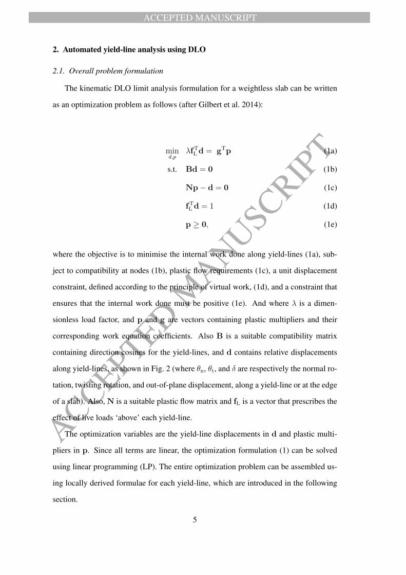
The kinematic DLO limit analysis formulation for a weightless slab can be written

as an optimization problem as follows (after Gilbert et al. 2014):

mind,p

λfTL d = gTp (1a)

s.t. Bd = 0 (1b)

Np− d = 0 (1c)

fTL d = 1 (1d)

p ≥ 0, (1e)

where the objective is to minimise the internal work done along yield-lines (1a), sub-

ject to compatibility at nodes (1b), plastic flow requirements (1c), a unit displacement

constraint, defined according to the principle of virtual work, (1d), and a constraint that

ensures that the internal work done must be positive (1e). And where λ is a dimen-

sionless load factor, and p and g are vectors containing plastic multipliers and their

corresponding work equation coefficients. Also B is a suitable compatibility matrix

containing direction cosines for the yield-lines, and d contains relative displacements

along yield-lines, as shown in Fig. 2 (where θn, θt, and δ are respectively the normal ro-

tation, twisting rotation, and out-of-plane displacement, along a yield-line or at the edge

of a slab). Also, N is a suitable plastic flow matrix and fL is a vector that prescribes the

effect of live loads ‘above’ each yield-line.

The optimization variables are the yield-line displacements in d and plastic multi-

pliers in p. Since all terms are linear, the optimization formulation (1) can be solved

using linear programming (LP). The entire optimization problem can be assembled us-

ing locally derived formulae for each yield-line, which are introduced in the following

section.

5

ACCEPTED MANUSCRIPT

ACCEPTED

MA

NU

SCRIP

T

(a) (b) (c)

Figure 2: Relative displacements at yield-line AB (assuming slab area ABCD moves to A′B′C′D′): (a)

normal rotation along yield-line; (b) twisting rotation; (c) out-of-plane translation

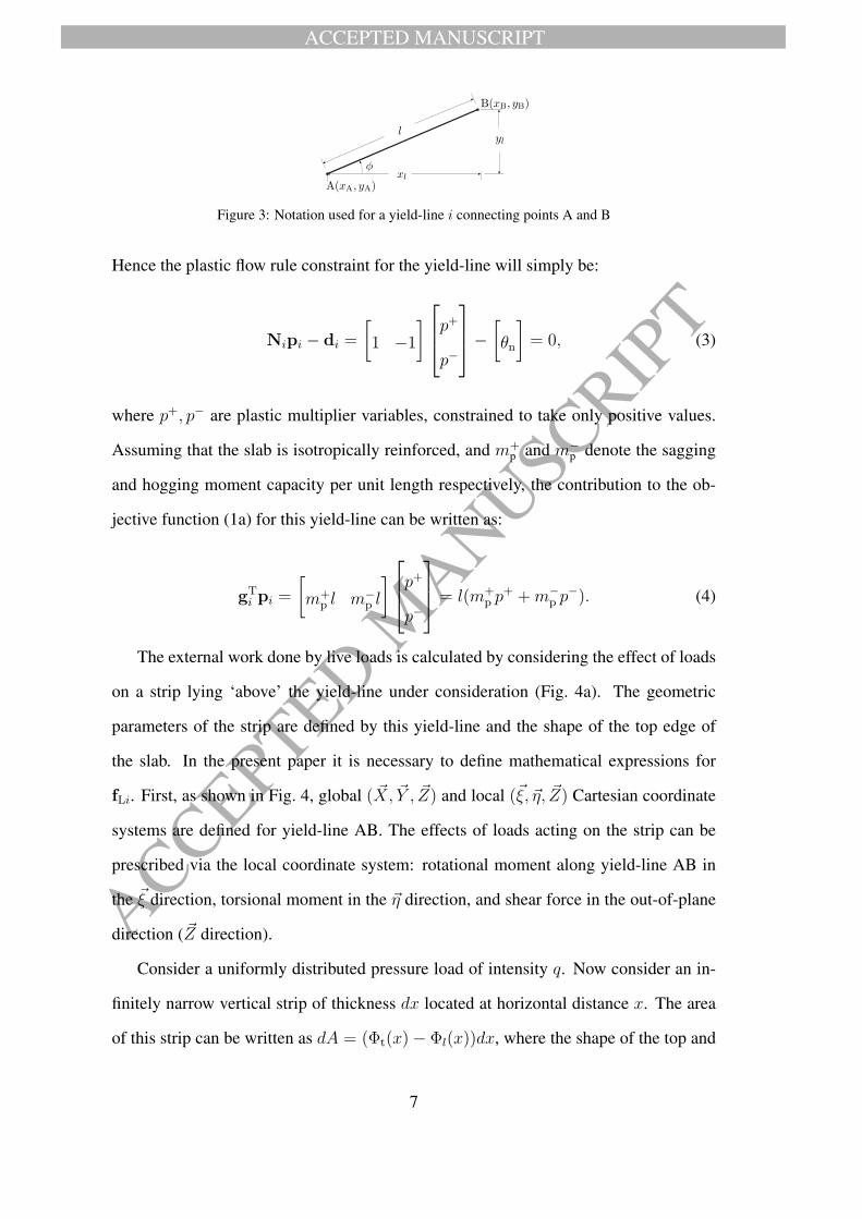
2.2. Terms for a single yield-line

For a yield-line i that connects two nodes A(xA, yA) and B(xB, yB), and inclined at

an angle φ to x axis, as shown in Fig. 3, let xl = xB − xA and yl = yB − yA. (Note

that in the interests of conciseness, the subscript i has been omitted, i.e. xl is used

rather than xli; this is repeated for all coefficients defined in this section). The length

of this yield-line is calculated using l =√

x2l + y2l , so cosφ = xl/l. Now assume

that the displacement variables in d for this yield-line are of the form [θn, θt, δ]T. The

contribution to the nodal compatibility constraint (1b) for this yield line is given by:

Bidi =

cosφ − sinφ 0

sinφ cosφ 0

0 l2

1

− cosφ sinφ 0

− sinφ − cosφ 0

0 l2

−1

θn

θt

δ

, (2)

where the first three rows in Bi contain the requisite nodal compatibility terms for node

A, which are, in order: rotational compatibility about the x axis and y axis, and out-of-

plane displacement compatibility. The last three rows contain the equivalent terms for

node B.

However, in yield-line analysis θt and δ will be zero except at free edges and along

symmetry planes; also internal work will only be associated with normal rotation θn.

6

ACCEPTED MANUSCRIPT

ACCEPTED

MA

NU

SCRIP

T

Figure 3: Notation used for a yield-line i connecting points A and B

Hence the plastic flow rule constraint for the yield-line will simply be:

Nipi − di =

[

1 −1

]

p+

p−

−

[

θn

]

= 0, (3)

where p+, p− are plastic multiplier variables, constrained to take only positive values.

Assuming that the slab is isotropically reinforced, and m+p and m−

p denote the sagging

and hogging moment capacity per unit length respectively, the contribution to the ob-

jective function (1a) for this yield-line can be written as:

gTi pi =

[

m+p l m−

p l

]

p+

p−

= l(m+

p p+ +m−

p p−). (4)

The external work done by live loads is calculated by considering the effect of loads

on a strip lying ‘above’ the yield-line under consideration (Fig. 4a). The geometric

parameters of the strip are defined by this yield-line and the shape of the top edge of

the slab. In the present paper it is necessary to define mathematical expressions for

fLi. First, as shown in Fig. 4, global ( ~X, ~Y , ~Z) and local (~ξ, ~η, ~Z) Cartesian coordinate

systems are defined for yield-line AB. The effects of loads acting on the strip can be

prescribed via the local coordinate system: rotational moment along yield-line AB in

the ~ξ direction, torsional moment in the ~η direction, and shear force in the out-of-plane

direction (~Z direction).

Consider a uniformly distributed pressure load of intensity q. Now consider an in-

finitely narrow vertical strip of thickness dx located at horizontal distance x. The area

of this strip can be written as dA = (Φt(x)− Φl(x))dx, where the shape of the top and

7

ACCEPTED MANUSCRIPT

ACCEPTED

MA

NU

SCRIP

T(a) (b)

Figure 4: Computing the effect of loads ‘above’ yield-line AB

bottom edges of the strip are defined by y = Φt(x) and y = Φl(x) respectively. The

magnitude of the pressure load on the whole strip can now be written as:

fi =

[

0, 0, −

∫ xB

xA

qdA

]T

. (5)

To determine the moment caused by the external load it is necessary to calculate

the distance vector ~r from the mid-point of line AB to the centroid of the load, where

~r : r =

[

xs − xc, ys − yc, 0

]T

, and where the centroid of the infinitely thin strip

is located at (xs, ys), and the mid-point of AB is located at (xc, yc). Thus the moment

caused by load on the whole strip above AB will be:

mi =

[∫

AB

q (yc − ys) dA,

∫

AB

q (xs − xc) dA, 0

]T

. (6)

By combining (5) and (6), the effects of the live load can thus be written as:

fGLi = q

∫

AB

(yc − ys) dA

∫

AB

(xs − xc) dA

−

∫

AB

dA

= q

∫ xB

xA

Λx(x)dx

∫ xB

xA

Λy(x)dx

−

∫ xB

xA

Λz(x)dx

, (7)

8

ACCEPTED MANUSCRIPT

ACCEPTED

MA

NU

SCRIP

T

where,

Λx(x) = (Φt(x)− Φl(x))yc −Φ2

t (x)− Φ2l (x)

2, (8a)

Λy(x) = (x− xc) (Φt(x)− Φl(x)), (8b)

Λz(x) = Φt(x)− Φl(x). (8c)

Λx, Λy, and Λz are unit-length moment and unit-length area functions with respect to

x in the global coordinate system, that respectively describe the first moment of area on

~X , the first moment of the area on ~Y , and the area per unit length in direction ~X for the

strip ‘above’ the yield-line. In addition, let Γx =

∫ xB

xA

Λxdx, Γy =

∫ xB

xA

Λydx, and Γz =

−

∫ xB

xA

Λzdx represent the unit live load effect. Note that the yield-line displacements

are defined in a local coordinate system, and it is thus necessary to apply a coordinate

transformation to obtain the requisite values:

fLi = q

cosφ sinφ 0

− sinφ cosφ 0

0 0 1

Γx

Γy

Γz

. (9)

3. Geometry optimization: basic formulation

In geometry optimization, in addition to the original variables (the displacements θn,

θt, δ in d and plastic multipliers p+ and p− in p), nodal positions xA, xB, yA, yB are

also considered as optimization variables. Also, with respect to the original optimiza-

tion formulation, the objective function (1a), nodal compatibility constraint (1b), and

unit displacement constraint (1d) now become non-linear, thus leading to a non-linear

programming (NLP) problem. To solve this problem efficiently, the first and second

derivatives of the objective function and constraints can be derived analytically, and ef-

ficient non-linear optimization packages such as IPOPT (Vigerske and Wachter 2013)

can be utilized. In the following section, mathematical expressions for the geometry

9

ACCEPTED MANUSCRIPT

ACCEPTED

MA

NU

SCRIP

T

optimization problem are given, including the first derivatives with respect to the opti-

mization variables (i.e., xA, yA, xB, yB, θn, θt, δ, p+, p−); second derivatives are provided

in Appendix A.

3.1. First derivative terms

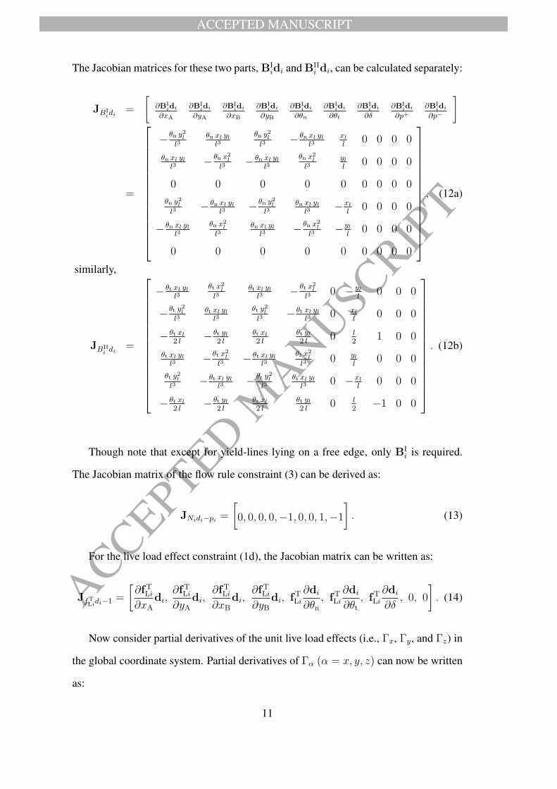
The gradient of the objective function and Jacobian matrices of the constraints are

the first derivatives required to solve the NLP problem. Assuming that the optimiza-

tion variables are in the form [xA, yA, xB, yB, θn, θt, δ, p+, p−] then the gradient of the

objective function (4) can be obtained as:

λ =

[

−λxl

l2, −

λyll2

,λxl

l2,λyll2

, 0, 0, 0, m+p l, m−

p l

]T

. (10)

Now consider the nodal compatibility constraint. As twisting rotation and out-of-

plane displacement will be zero for yield-lines which do not lie on free (or symmetry)

boundaries, it is efficient to treat these differently; thus compatibility matrix Bi can

conveniently be divided into two parts, Bi = BIi +BII

i , where:

BIi =

cosφ 0 0

sinφ 0 0

0 0 0

− cosφ 0 0

− sinφ 0 0

0 0 0

, BIIi =

0 − sinφ 0

0 cosφ 0

0 l2

1

0 sinφ 0

0 − cosφ 0

0 l2

−1

. (11)

10

ACCEPTED MANUSCRIPT

ACCEPTED

MA

NU

SCRIP

T

The Jacobian matrices for these two parts, BIidi and BII

i di, can be calculated separately:

JBIidi =

[

∂BIidi

∂xA

∂BIidi

∂yA

∂BIidi

∂xB

∂BIidi

∂yB

∂BIidi

∂θn

∂BIidi

∂θt

∂BIidi

∂δ

∂BIidi

∂p+∂BI

idi

∂p−

]

=

−θn y2

l

l3θn xl yl

l3θn y2

l

l3− θn xl yl

l3xl

l0 0 0 0

θn xl yll3

−θn x2

l

l3− θn xl yl

l3θn x2

l

l3yll

0 0 0 0

0 0 0 0 0 0 0 0 0

θn y2l

l3− θn xl yl

l3−

θn y2l

l3θn xl yl

l3−xl

l0 0 0 0

− θn xl yll3

θn x2l

l3θn xl yl

l3−

θn x2l

l3−yl

l0 0 0 0

0 0 0 0 0 0 0 0 0

, (12a)

similarly,

JBIIidi =

− θt xl yll3

θt x2l

l3θt xl yl

l3−

θt x2l

l30 −yl

l0 0 0

−θt y2ll3

θt xl yll3

θt y2ll3

− θt xl yll3

0 xl

l0 0 0

− θt xl

2 l− θt yl

2 lθt xl

2 lθt yl2 l

0 l2

1 0 0

θt xl yll3

−θt x2

l

l3− θt xl yl

l3θt x2

l

l30 yl

l0 0 0

θt y2ll3

− θt xl yll3

−θt y2ll3

θt xl yll3

0 −xl

l0 0 0

− θt xl

2 l− θt yl

2 lθt xl

2 lθt yl2 l

0 l2

−1 0 0

. (12b)

Though note that except for yield-lines lying on a free edge, only BIi is required.

The Jacobian matrix of the flow rule constraint (3) can be derived as:

JNidi−pi =

[

0, 0, 0, 0,−1, 0, 0, 1,−1

]

. (13)

For the live load effect constraint (1d), the Jacobian matrix can be written as:

JfTLidi−1 =

[

∂fTLi∂xA

di,∂fTLi∂yA

di,∂fTLi∂xB

di,∂fTLi∂yB

di, fTLi∂di

∂θn, fTLi

∂di

∂θt, fTLi

∂di

∂δ, 0, 0

]

. (14)

Now consider partial derivatives of the unit live load effects (i.e., Γx, Γy, and Γz) in

the global coordinate system. Partial derivatives of Γα (α = x, y, z) can now be written

as:

11

ACCEPTED MANUSCRIPT

ACCEPTED

MA

NU

SCRIP

T

∂Γα

∂xA

=∂

∂xA

∫ xB

xA

Λαdx = −Λα +

∫ xB

xA

∂Λα

∂xA

dx, (15a)

∂Γα

∂yA=

∂

∂yA

∫ xB

xA

Λαdx =

∫ xB

xA

∂Λα

∂yAdx, (15b)

∂Γα

∂xB

=∂

∂xB

∫ xB

xA

Λαdx = Λα +

∫ xB

xA

∂Λα

∂xB

dx, (15c)

∂Γα

∂yB=

∂

∂yB

∫ xB

xA

Λαdx =

∫ xB

xA

∂Λα

∂yBdx. (15d)

Next consider the local coordinate system. Note that in (14), the partial derivatives

with respect to the nodal coordinates (i.e., the first four terms) have very similar expres-

sions, and those with respect to yield-line displacements (i.e., the fifth to seventh terms)

are similar. In the interests of conciseness, only the first and fifth terms (i.e.,∂fTLi

∂xAdi and

fTLi∂di

∂θn) are shown:

∂fTLi∂xA

di = qδ∂

∂xA

Γz − qθt

(

Γy

l−

xl∂

∂xAΓy

l+

yl∂

∂xAΓx

l−

x2l Γy

l3+

yl xl Γx

l3

)

−qθn

(

Γx

l−

xl∂

∂xAΓx

l−

yl∂

∂xAΓy

l−

x2l Γx

l3−

yl xl Γy

l3

)

, (16a)

fTLi∂di

∂θn= q

xl Γx

l+ q

yl Γy

l. (16b)

3.2. Second derivative terms

Second derivatives (i.e., the Hessian matrices) can sometimes be approximated us-

ing Quasi-Newton methods (e.g., the BFGS method described in Nocedal et al. 2006).

However, to ensure the NLP process is as efficient as possible, they are derived analyt-

ically in this paper. Details of the mathematical expressions for the second derivative

terms are given in Appendix A.

3.3. Assembling the entire problem

For a single yield-line, the analytical expressions for the first and second derivatives

have been derived, and thus the entire problem can be readily assembled. In the case

12

ACCEPTED MANUSCRIPT

ACCEPTED

MA

NU

SCRIP

T

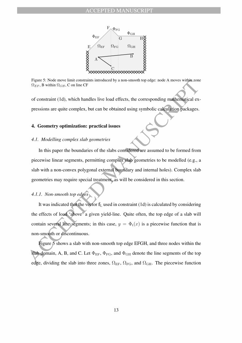
Figure 5: Node move limit constraints introduced by a non-smooth top edge: node A moves within zone

ΩEF , B within ΩGH , C on line CF

of constraint (1d), which handles live load effects, the corresponding mathematical ex-

pressions are quite complex, but can be obtained using symbolic calculation packages.

4. Geometry optimization: practical issues

4.1. Modelling complex slab geometries

In this paper the boundaries of the slabs considered are assumed to be formed from

piecewise linear segments, permitting complex slab geometries to be modelled (e.g., a

slab with a non-convex polygonal external boundary and internal holes). Complex slab

geometries may require special treatment, as will be considered in this section.

4.1.1. Non-smooth top edges

It was indicated that the vector fL used in constraint (1d) is calculated by considering

the effects of load ‘above’ a given yield-line. Quite often, the top edge of a slab will

contain several line segments; in this case, y = Φt(x) is a piecewise function that is

non-smooth or discontinuous.

Figure 5 shows a slab with non-smooth top edge EFGH, and three nodes within the

slab domain, A, B, and C. Let ΦEF, ΦFG, and ΦGH denote the line segments of the top

edge, dividing the slab into three zones, ΩEF, ΩFG, and ΩGH. The piecewise function

13

ACCEPTED MANUSCRIPT

ACCEPTED

MA

NU

SCRIP

T

Φt(x) for the top edge can be written as:

Φt(x) =

ΦEF(x), xE ≤ x ≤ xF

ΦFG(x), xF ≤ x ≤ xG

ΦFH(x), xG ≤ x ≤ xH

. (17)

The unit-length moment and area functions Λα(α = x, y, z) are now expressed as:

Λα(x) =

ΛEFα (x), xE ≤ x ≤ xF

ΛFGα (x), xF ≤ x ≤ xG

ΛGHα (x), xG ≤ x ≤ xH

, (18)

where ΛEFα , ΛFG

α , and ΛGHα are unit-length moment and area functions in zones ΩEF,

ΩFG, and ΩGH, respectively. The first derivatives of the unit live load effect Γx, Γy, and

Γz can be derived using (15). For example, for node A of yield-line AB:

∂Γα

∂xA

= −ΛEFα +

∫ xF

xA

∂ΛEFα

∂xA

dx+

∫ xG

xF

∂ΛFGα

∂xA

dx+

∫ xB

xG

∂ΛGHα

∂xA

dx, (19)

∂Γα

∂yA=

∫ xF

xA

∂ΛEFα

∂yAdx+

∫ xG

xF

∂ΛFGα

∂yAdx+

∫ xB

xG

∂ΛGHα

∂yAdx. (20)

These formulae are valid only when node A lies within zone ΩEF, so that node A

must be restricted to lie within this zone. Also, node C must be restricted to lie on

line CF lying between ΩEF and ΩFG. Thus, when a slab has a non-smooth top edge,

each node must be restricted to lie within the zone in which it currently lies, with only

vertical movement permitted in the case of nodes lying directly below a non-smooth

point. This can be considered to be a limitation of the method, as currently implemented.

(However, in practice it may sometimes be possible to overcome this limitation simply

by re-orientating the slab, so that a simple edge is uppermost; e.g., the slab in Fig. 5 can

be rotated 180 to have a smooth top edge.)

14

ACCEPTED MANUSCRIPT

ACCEPTED

MA

NU

SCRIP

T

4.1.2. Slab with holes

When a hole is present, calculating the effects of live loads is complicated by the

need to exclude areas occupied by the hole in the vertical strip lying above a given

yield-line. This has not been considered in the formulae introduced above. A means

of incorporating holes using the presented formulae is to use domain decomposition.

When using decomposition a slab domain can be divided into several sub-domains in

which the holes are excluded; details are provided in Appendix B.

4.1.3. Non-convex polygonal slab

When moving nodes in a non-convex polygonal slab, a yield-line can potentially

be moved so as to cross a slab boundary. This can either be addressed via domain

decomposition (which involves dividing non-convex domains into several convex sub-

domains) or by introducing additional constraints (not considered here). In the examples

considered in this paper no yield-lines exhibiting the described behaviour were found to

be present, and thus no action was necessary.

4.2. Inherited issues

In the truss rationalization formulation presented by He and Gilbert (2015), steps

were taken to address a number of practical issues, for example, restrictions on the

movement of nodes, merging of nodes in close proximity, etc; these issues are addressed

here using the same basic techniques.

4.2.1. Node move limits

Because of the non-convex nature of the optimization problem, the NLP solver (i.e.,

IPOPT) may report an unstable status. Furthermore, clearly nodes must be restricted

from only lying within the geometry of the slab. To address these issues, in the the

truss rationalization formulation (He and Gilbert 2015) node move limits were active

for every node. In this paper, the same basic approach is used; firstly, the nodes can

only move within regions defined to be a function of nodal spacing; secondly, line and

domain constraints are imposed according to the geometry of the slab.

15

ACCEPTED MANUSCRIPT

ACCEPTED

MA

NU

SCRIP

T

In the first step, assume that the nodal coordinates of a node are written in R3 as

ν = [x, y, 1]T (as per the truss rationalization formulation (He and Gilbert 2015), the

redundant ‘1’ is used to condense the mathematical expression). Consider two adjacent

nodes A and B, and let r = 12‖ν0

B − ν0A‖2 be half the distance between them, ǫ be a

gap used to avoid generating a zero length yield-line, and r be a program parameter

that defines the maximum node move limit for all nodes. The node move limit is then

obtained as r∗ = minr − ǫ, r.

In the second step, nodes on slab boundaries must be restricted to lie on boundary

lines in order to retain the slab geometry; therefore, line constraints are imposed on

these nodes. As in the truss rationalization formulation (He and Gilbert 2015), let T

be the coefficient vector of a line so that the line constraint is written as Tν = 0; for

domain constraints, an inequality constraint is instead used (also note that T can now

be a matrix to describe several lines).

4.2.2. Merging nodes

During the rationalization process, certain nodes may migrate towards each other.

A node merge process was introduced in the truss rationalization formulation (He and

Gilbert 2015), and this approach is also adopted here: first, the nodes are grouped based

on distances; then, merging every individual group is attempted, provided that the re-

sulting yield-line pattern is validated numerically.

4.2.3. Extracting yield-line patterns from DLO

The rationalization process requires an initial yield-line pattern to be extracted from

a DLO analysis. Typically, such a pattern is obtained by removing yield-lines having

rotations (θn) that are smaller than a prescribed threshold value (except for boundary

yield-lines, which are not removed). To ensure a reasonable threshold number is chosen,

the extracted yield-line pattern will be used as the basis of a new analysis, and the

load factor compared with that obtained originally. If these are not within a prescribed

tolerance then the threshold value should be progressively reduced until the load factor

16

ACCEPTED MANUSCRIPT

ACCEPTED

MA

NU

SCRIP

T

obtained is within the prescribed tolerance, and a usable initial yield-line pattern is

obtained.

4.2.4. Crossovers

Typically, yield-line patterns obtained using DLO will include crossover points

where two or more yield-lines intersect that do not coincide with nodes. As with the

truss rationalization formulation (He and Gilbert 2015), nodes can be added at these

locations using a nested-loop strategy: an inner loop performs geometry optimization

and, whenever the inner loop finishes, crossover nodes are created in the outer loop, and

then a further cycle of the inner loop is performed. The whole process is repeated until

no crossover points are found.

5. Geometry optimization: full formulation

Consider a slab that comprises N = 1, 2, ..., n nodes, with node subsets NL and

ND denoting those nodes that lie on the boundary lines and those close to domain bound-

aries, respectively. The full optimization problem, now considering nodal move limits,

can be written as:

minx,y,d,p

λfTL d = gTp (21a)

s.t. Bd = 0 (21b)

Np− d = 0 (21c)

fTL d = 1 (21d)

p ≥ 0 (21e)

∥

∥

νj − ν0j

∥

∥

2

2≤ (r∗)2 for all j ∈ N (21f)

TLj νj = 0 for all j ∈ N

L (21g)

Tνj ≥ 0 for all j ∈ ND (21h)

xlb ≤ x ≤ xub (21i)

ylb ≤ y ≤ yub, (21j)

17

ACCEPTED MANUSCRIPT

ACCEPTED

MA

NU

SCRIP

T

where xlb, xub, ylb, and yub are the lower and upper bounds of the nodal positions,

which are calculated by taking account of the practical issues that affect node move-

ments (e.g. limits imposed to address non-smooth top edges).

6. Numerical examples

In this section, the efficacy of the proposed rationalization technique is demonstrated

by applying it to various numerical example problems. Unless stated otherwise, the

slabs considered have unit moment resistance per unit length, and are subjected to a

uniform pressure load of unit intensity. Also, a default node merge radius of 0.25× the

x or y-nodal spacing in the original DLO analysis was assumed. To solve both the LP

and NLP problems, the IPOPT 3.11.0 (Vigerske and Wachter 2013) interior point opti-

mization solver was used, with a maximum of 500 iterations allowed. All calculations

were performed using MATLAB2013a running under the Microsoft Windows 7 operat-

ing system on an Intel i5-2310 powered desktop with 6G RAM. Finally, unless stated

otherwise, the line thickness of the plotted yield-lines are proportional to the yield-line

rotation.

6.1. Gilbert et al. (2014) examples

In Gilbert et al. (2014), the proposed DLO-based automatic yield-line analysis

method was applied to several slab problems. These examples will now be revisited,

with the DLO derived yield-line patterns now rationalized using the new procedure.

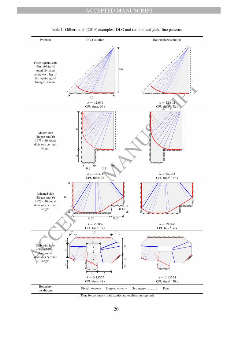
Thus in Table 1, both standard DLO and rationalized solutions are presented.

It is evident that the rationalization process successfully simplifies the yield-line pat-

terns, and also improves the solutions (i.e. reduces the load factors). The linear nature

of the DLO formulation means that large-scale problems, e.g. involving millions of

potential yield-line discontinuities, can be solved without difficulty. In comparison the

NLP problem associated with the geometry optimization formulation is considerably

more difficult to solve. However, fortunately the size of the problem which needs to be

18

ACCEPTED MANUSCRIPT

ACCEPTED

MA

NU

SCRIP

T

solved in the proposed procedure is much reduced, containing several orders of magni-

tude fewer yield-line discontinuities. Table 2, shows how the CPU time increases with

increasing number of nodes and yield-lines, for the fixed square slab problem. Also Fig-

ure 6 shows solutions for this problem for the 60 and 120 nodal division cases (nodes

are shown but, for sake of clarity, a constant yield-line line thicknesses has been used).

It can be observed that the rationalized patterns contain far fewer nodes and yield-lines

than present in the final DLO solutions.

Alternatively, fewer nodes can be employed in the initial DLO problem to ensure

that even simpler solutions are obtained; such solutions are potentially attractive to

practitioners, who may require yield-line patterns which are easy to visualise and to

hand-check. Thus, Fig. 7 shows solutions for the slab with alcoves problem with vari-

ous nodal divisions. The coarsest solution corresponds to an extremely simple yield-line

pattern but is still within 5% of the extrapolated solution (of 35.230) given in Gilbert

et al. (2014), which can be considered for all practical purposes to be exact. Also, be-

cause a very coarse initial grid has been used, the solution could be obtained in a fraction

of a second.

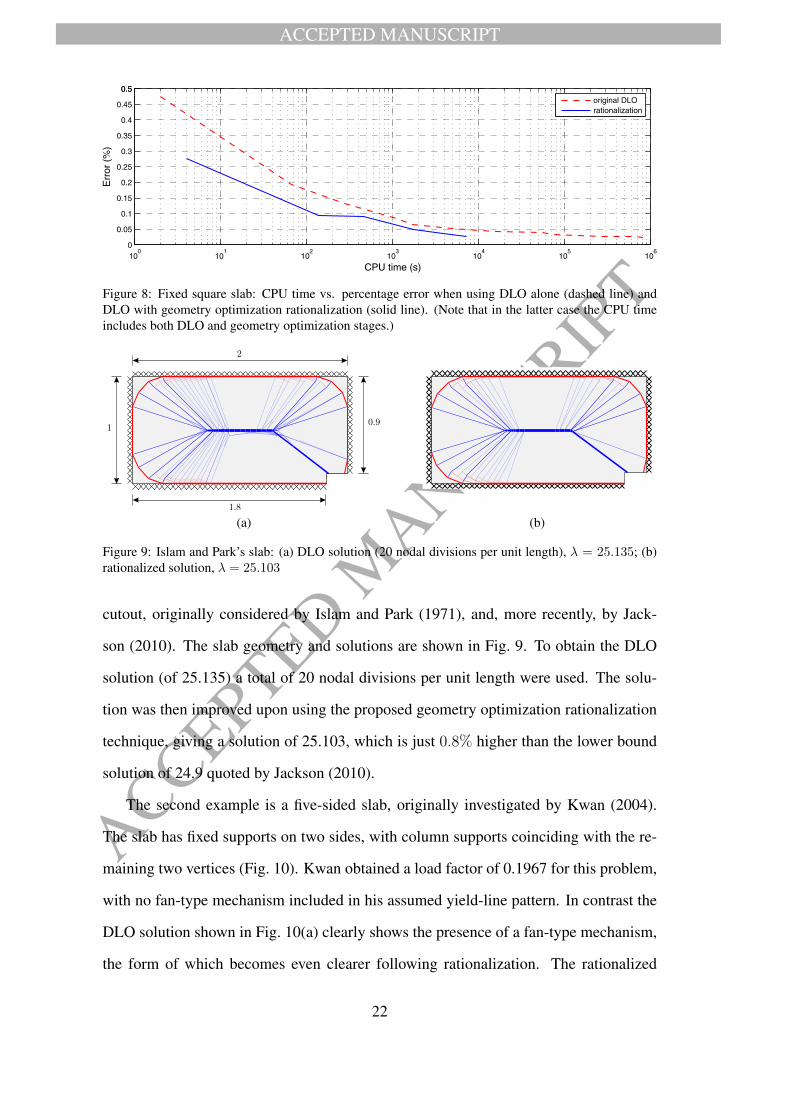
Finally, since the geometry optimization rationalization step will generally improve

the numerical solution (i.e. will reduce the load factor), it is of interest to ascertain

whether it can be used to reduce the total CPU time required to achieve a solution of

a given accuracy. Figure 8 presents results for the fixed square slab problem, showing

that use of the rationalization step can indeed reduce the CPU time required to give a

solution of a given accuracy.

6.2. Irregular slabs with corner fans

It is well-understood that fan-type mechanisms develop at clamped corners. How-

ever, fan-type mechanisms have proved difficult to identify using traditional automated

yield-line analysis methods (e.g. Munro and Da Fonseca 1978; Johnson 1994). It is

therefore of interest to consider two representative examples here.

The first example comprises a rectangular slab with fixed supports and a corner

19

ACCEPTED MANUSCRIPT

ACCEPTED

MA

NU

SCRIP

T

Table 1: Gilbert et al. (2014) examples: DLO and rationalized yield-line patterns

Problem DLO solution Rationalized solution

Fixed square slab

(Fox 1974): 40

nodal divisions

along each leg of

the right-angled

triangle domain

λ = 42.934 λ = 42.892CPU time: 66 s CPU time†: 72 s

Alcove slab

(Regan and Yu

1973): 40 nodal

divisions per unit

length

λ = 35.411 λ = 35.353CPU time: 9 s CPU time†: 37 s

Indented slab

(Regan and Yu

1973): 40 nodal

divisions per unit

length

λ = 29.062 λ = 29.026CPU time: 19 s CPU time†: 6 s

Slab with hole

(Olsen 1998):

five nodal

divisions per unit

length

λ = 0.13557 λ = 0.13554CPU time: 48 s CPU time†: 70 s

Boundary

conditionsFixed: Simple: Symmetry: Free:

†: Time for geometry optimization rationalization step only

20

ACCEPTED MANUSCRIPT

ACCEPTED

MA

NU

SCRIP

T

Table 2: Fixed square slab: influence of number of DLO nodal divisions

DLO Geometry optimization rationalization

Nodal

divisions

No. of

nodes

No. of

yield-lines

Load factor

(error)

CPU

time

No. of

nodes

No. of

yield-lines

Load factor

(error)

CPU

time

Total

CPU

cost†

20 291 28037 43.055 (0.48%) 2 9 13 42.969 (0.28%) 2 4

40 981 285204 42.934 (0.19%) 66 30 52 42.892 (0.10%) 72 138

60 2071 1041621 42.908 (0.13%) 278 53 88 42.890 (0.10%) 174 264

80 3561 2430190 42.887 (0.09%) 1105 201 418 42.873 (0.05%) 655 1760

100 5451 4496066 42.879 (0.06%) 1704 487 1118 42.867 (0.04%) 1416 3120

120 7741 7258302 42.874 (0.05%) 4845 774 2069 42.863 (0.03%) 2304 7149

†: Time includes both DLO and geometry optimization stages

(a) (b)

Figure 6: Fixed square slab: comparison of DLO and rationalized yield-line patterns for: (a) 60 nodal

divisions; (b) 120 nodal divisions

(a) 20 nodal divisions

λ = 35.529(b) 10 nodal divisions

λ = 35.808(c) 5 nodal divisions

λ = 36.921

Figure 7: Slab with alcoves: coarse resolution DLO solutions suitable for hand checking (left: initial

DLO nodal grid; right: rationalized solution)

21

ACCEPTED MANUSCRIPT

ACCEPTED

MA

NU

SCRIP

TFigure 8: Fixed square slab: CPU time vs. percentage error when using DLO alone (dashed line) and

DLO with geometry optimization rationalization (solid line). (Note that in the latter case the CPU time

includes both DLO and geometry optimization stages.)

(a) (b)

Figure 9: Islam and Park’s slab: (a) DLO solution (20 nodal divisions per unit length), λ = 25.135; (b)

rationalized solution, λ = 25.103

cutout, originally considered by Islam and Park (1971), and, more recently, by Jack-

son (2010). The slab geometry and solutions are shown in Fig. 9. To obtain the DLO

solution (of 25.135) a total of 20 nodal divisions per unit length were used. The solu-

tion was then improved upon using the proposed geometry optimization rationalization

technique, giving a solution of 25.103, which is just 0.8% higher than the lower bound

solution of 24.9 quoted by Jackson (2010).

The second example is a five-sided slab, originally investigated by Kwan (2004).

The slab has fixed supports on two sides, with column supports coinciding with the re-

maining two vertices (Fig. 10). Kwan obtained a load factor of 0.1967 for this problem,

with no fan-type mechanism included in his assumed yield-line pattern. In contrast the

DLO solution shown in Fig. 10(a) clearly shows the presence of a fan-type mechanism,

the form of which becomes even clearer following rationalization. The rationalized

22

ACCEPTED MANUSCRIPT

ACCEPTED

MA

NU

SCRIP

T(a) (b)

Figure 10: Kwan’s five sided slab: (a) DLO (five nodal divisions per unit length), λ = 0.18849; (b)

rationalized solution, λ = 0.18775

solution of 0.18775 is some 4.5% less than the solution obtained by Kwan.

6.3. Cruciform slab

Johnson (1994) investigated the critical yield-line patterns for a simply supported

cruciform slab of various dimensions; see Fig. 11. He identified three yield-line pat-

terns: the ‘crossed rectangular slab’ mode for low values of x; the ‘modified square

slab’ mode for intermediate values of x; and the ‘corner lever’ mode for high values of

x. More recently, Jackson (2010) revisited the problem, though presented only lower

bound solutions and ‘yield-line indicators’ (obtaining yield-line solutions using his pro-

posed method involved human-intervention, and would likely have been labour inten-

sive to perform for multiple geometries).

However, here the rationalization procedure has been used to automatically generate

clear patterns for the cruciform slab problem; see Table 3. In the first two modes, a fan-

type mechanism can clearly be observed near the concave corners.

7. Conclusions

• For many decades the yield-line method of analysis for reinforced concrete slabs

eluded systematic automation. This has finally now been achieved, via the dis-

continuity layout optimization (DLO) procedure, which can rapidly obtain high

23

ACCEPTED MANUSCRIPT

ACCEPTED

MA

NU

SCRIP

TFigure 11: Cruciform slab: problem specification (L = 1)

accuracy solutions for slabs of arbitrary geometry. However, the use of a fixed

nodal grid means that the corresponding yield-line patterns can be somewhat more

complex in form than is necessary.

• To address this, in this paper a post-processing rationalization step which involves

the use of geometry optimization to adjust the positions of nodes has been pro-

posed. As the yield-line patterns obtained via DLO normally contain only a rel-

atively small number of nodes and yield-lines, solutions to the inherently non-

linear geometry optimization problem can be obtained relatively rapidly using an

interior point solver.

• Benefits of the proposed post-processing rationalization step are that the ratio-

nalized solutions are generally both simpler in form and more accurate than raw

DLO solutions. From the point of view of practitioners, this means that a rel-

atively coarse initial nodal grid can be used to provide solutions of engineering

accuracy in a matter of seconds. These solutions are also easier to check by hand

(if required) and appear more convincing than raw DLO solutions. This demon-

strates the practical usefulness of the proposed procedure.

8. Acknowledgements

The first author acknowledges the doctoral studies scholarship provided by the Fac-

ulty of Engineering at the University of Sheffield.

24

ACCEPTED MANUSCRIPT

ACCEPTED

MA

NU

SCRIP

T

Table 3: Cruciform slab: rationalized yield-line patterns for various x/L ratios

Failure mode Rationalized solutions

Crossed

rectangular

slab mode

x/L = 0.2, λ = 71.940 x/L = 0.3, λ = 38.344

Modified

square slab

mode

x/L = 0.4, λ = 24.248 x/L = 0.5, λ = 16.637

Corner lever

mode

x/L = 0.8, λ = 7.1549 x/L = 0.9, λ = 6.2575

25

ACCEPTED MANUSCRIPT

ACCEPTED

MA

NU

SCRIP

T

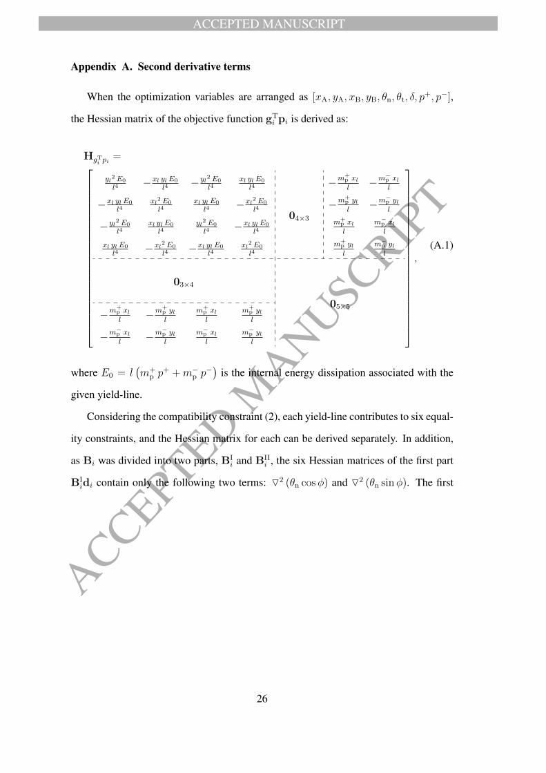
Appendix A. Second derivative terms

When the optimization variables are arranged as [xA, yA, xB, yB, θn, θt, δ, p+, p−],

the Hessian matrix of the objective function gTi pi is derived as:

HgTipi =

yl2 E0

l4−xl yl E0

l4−yl

2 E0

l4xl yl E0

l4

04×3

−m+

p xl

l−

m−p xl

l

−xl yl E0

l4xl

2 E0

l4xl yl E0

l4−xl

2 E0

l4−

m+p yll

−m−

p yll

−yl2 E0

l4xl yl E0

l4yl

2 E0

l4−xl yl E0

l4m+

p xl

l

m−p xl

l

xl yl E0

l4−xl

2 E0

l4−xl yl E0

l4xl

2 E0

l4m+

p yll

m−p yll

03×4

05×5

−m+

p xl

l−

m+p yll

m+p xl

l

m+p yll

−m−

p xl

l−

m−p yll

m−p xl

l

m−p yll

,(A.1)

where E0 = l(

m+p p+ +m−

p p−)

is the internal energy dissipation associated with the

given yield-line.

Considering the compatibility constraint (2), each yield-line contributes to six equal-

ity constraints, and the Hessian matrix for each can be derived separately. In addition,

as Bi was divided into two parts, BIi and BII

i , the six Hessian matrices of the first part

BIidi contain only the following two terms:

2 (θn cosφ) and 2 (θn sinφ). The first

26

ACCEPTED MANUSCRIPT

ACCEPTED

MA

NU

SCRIP

T

term 2 (θn cosφ) can be found to be:

2 (θn cosφ) =

−3θnxly

2l

l5

symmetrical

05×4

−θnyl(−2x2

l+y2

l)

l5θnxl(−x2

l+2y2

l)

l5

3θnxly2l

l5θnyl(−2x2

l+y2

l)

l5−

3θnxly2l

l5

θnyl(−2x2l+y2

l)

l5−

θnxl(−x2l+2y2

l)

l5−

θnyl(−2x2l+y2

l)

l5θnxl(−x2

l+2y2

l)

l5

−yll3

xlyll3

y2l

l3−xlyl

l30

04×5 04×4

,(A.2)

which is a symmetrical 9 × 9 matrix. The second term has a similar form (for sake of

conciseness not shown here).

Now consider the second part, BIIi di; its Hessian matrices contain the following four

terms: 2 (θt sinφ), 2 (θt cosφ),

2(

l2θt + δ

)

, and 2(

l2θt − δ

)

. Clearly, the first two

terms can be obtained by simply replacing θn with θt in 2 (θn sinφ) and

2 (θn cosφ),

and then reordering the rows and columns accordingly. The third and fourth terms can

be found to be:

2

(

l

2θt + δ

)

= 2

(

l

2θt − δ

)

=

θt yl2

2 l3

symmetrical

06×3

− θt xl yl2 l3

θt xl2

2 l3

− θt yl2

2 l3θt xl yl2 l3

θt yl2

2 l3

θt xl yl2 l3

− θt xl2

2 l3− θt xl yl

2 l3θt xl

2

2 l3

0 0 0 0 0

− xl

2 l− yl

2 lxl

2 lyl2 l

0 0

03×6 03×3

.

(A.3)

27

ACCEPTED MANUSCRIPT

ACCEPTED

MA

NU

SCRIP

T

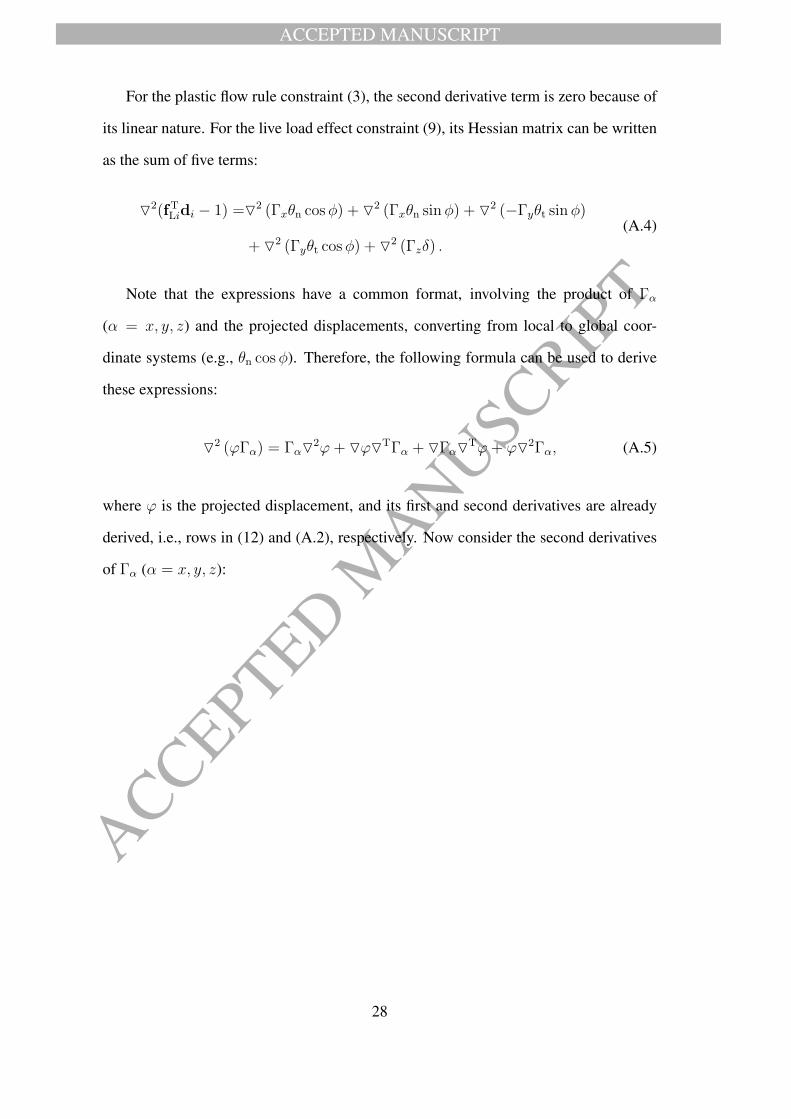
For the plastic flow rule constraint (3), the second derivative term is zero because of

its linear nature. For the live load effect constraint (9), its Hessian matrix can be written

as the sum of five terms:

2(fTLidi − 1) =

2 (Γxθn cosφ) + 2 (Γxθn sinφ) +

2 (−Γyθt sinφ)

+ 2 (Γyθt cosφ) +

2 (Γzδ) .

(A.4)

Note that the expressions have a common format, involving the product of Γα

(α = x, y, z) and the projected displacements, converting from local to global coor-

dinate systems (e.g., θn cosφ). Therefore, the following formula can be used to derive

these expressions:

2 (ϕΓα) = Γα

2ϕ+ ϕTΓα + ΓαTϕ+ ϕ2Γα, (A.5)

where ϕ is the projected displacement, and its first and second derivatives are already

derived, i.e., rows in (12) and (A.2), respectively. Now consider the second derivatives

of Γα (α = x, y, z):

28

ACCEPTED MANUSCRIPT

ACCEPTED

MA

NU

SCRIP

T

∂2Γα

∂x2A

= −2∂Λα

∂xA

+

∫ xB

xA

∂2Λα

∂x2A

dx, (A.6a)

∂2Γα

∂yA∂xA

= −∂Λα

∂yA+

∫ xB

xA

∂2Λα

∂yA∂xA

dx, (A.6b)

∂2Γα

∂y2A=

∫ xB

xA

∂2Λα

∂y2Adx, (A.6c)

∂2Γα

∂xB∂xA

=∂Λα

∂xA

−∂Λα

∂xB

+

∫ xB

xA

∂2Λα

∂xB∂xA

dx, (A.6d)

∂2Γα

∂xB∂yA=

∂Λα

∂yA+

∫ xB

xA

∂2Λα

∂xB∂yAdx, (A.6e)

∂2Γα

∂x2B

= 2∂Λα

∂xB

+

∫ xB

xA

∂2Λα

∂x2B

dx, (A.6f)

∂2Γα

∂yB∂xA

= −∂Λα

∂yB+

∫ xB

xA

∂2Λα

∂yB∂xA

dx, (A.6g)

∂2Γα

∂yB∂yA=

∫ xB

xA

∂2Λα

∂yB∂yAdx, (A.6h)

∂2Γα

∂yB∂xB

=∂Λα

∂yB+

∫ xB

xA

∂2Λα

∂yB∂xB

dx, (A.6i)

∂2Γα

∂y2B=

∫ xB

xA

∂2Λα

∂y2Bdx. (A.6j)

(α = x, y, z)

Note that Γz is not a function of the displacement variables. The Hessian matrix of

Γα (α = x, y, z) can now readily be obtained, as can the full expression for (A.4). For

instance, considering (A.5), the fifth term 2 (Γzδ) can be written as:

2 (Γzδ) = Γz

2δ + δTΓz + ΓzTδ + δ2Γz

= δTΓz + ΓzTδ + δ2Γz

=

δ24×4Γz 04×2 4×1Γz 04×2

02×4

05×5T1×4Γz

02×4

,

(A.7)

29

ACCEPTED MANUSCRIPT

ACCEPTED

MA

NU

SCRIP

T

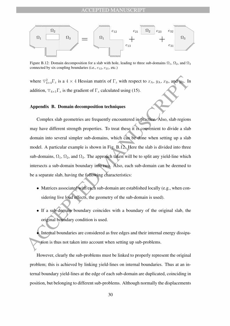
Figure B.12: Domain decomposition for a slab with hole, leading to three sub-domains Ω1, Ω2, and Ω3

connected by six coupling boundaries (i.e., e12, e21, etc.)

where 24×4Γz is a 4 × 4 Hessian matrix of Γz with respect to xA, yA, xB, and yB. In

addition, 4×1Γz is the gradient of Γz calculated using (15).

Appendix B. Domain decomposition techniques

Complex slab geometries are frequently encountered in practice. Also, slab regions

may have different strength properties. To treat these it is convenient to divide a slab

domain into several simpler sub-domains, which can be done when setting up a slab

model. A particular example is shown in Fig. B.12. Here the slab is divided into three

sub-domains, Ω1, Ω2, and Ω3. The approach taken will be to split any yield-line which

intersects a sub-domain boundary into two. Also, each sub-domain can be deemed to

be a separate slab, having the following characteristics:

• Matrices associated with each sub-domain are established locally (e.g., when con-

sidering live load effects, the geometry of the sub-domain is used).

• If a sub-domain boundary coincides with a boundary of the original slab, the

original boundary condition is used.

• Internal boundaries are considered as free edges and their internal energy dissipa-

tion is thus not taken into account when setting up sub-problems.

However, clearly the sub-problems must be linked to properly represent the original

problem; this is achieved by linking yield-lines on internal boundaries. Thus at an in-

ternal boundary yield-lines at the edge of each sub-domain are duplicated, coinciding in

position, but belonging to different sub-problems. Although normally the displacements

30

ACCEPTED MANUSCRIPT

ACCEPTED

MA

NU

SCRIP

T

at yield-lines are relative, at the edges of a domain (or sub-domain) these are relative to

the surrounding void domain, and hence can be considered to be absolute. Thus, assum-

ing the absolute displacements at the edges of sub-domain Ω1 and Ω2 are denoted θΩ1n ,

θΩ1t , and δΩ1, and at θΩ2

n , θΩ2t , and δΩ2 respectively, the required compatibility condition

can be written as follows:

θΩ1n + θΩ2

n − θBn = 0, (B.1a)

θΩ1t + θΩ2

t = 0, (B.1b)

δΩ1 + δΩ2 = 0, (B.1c)

where θBn is introduced to model the presence of a potential real yield-line at the bound-

ary (supplemented by corresponding plastic multiplier terms). Note that, in order to

avoid sign convention issues, all line directions are assumed to be identical. Thus if S

denotes the coefficient matrix for constraint B.1 then Sd = 0. Hence the compatibility

constraints for a problem where domain decomposition has been used can be written as:

Bαd = 0, for all α ∈ S, (B.2)

Sd = 0, (B.3)

where Bα is the compatibility matrix for sub-problem α, and where S is the set of all

sub-domains.

References

Anderheggen, E., Knopfel, H., 1972. Finite element limit analysis using linear pro-

gramming. International Journal of Solids and Structures 8, 1413–1431.

Bauer, S., Lackner, R., 2015. Gradient-based adaptive discontinuity layout optimization

for the prediction of strength properties in matrix-inclusion materials. Int. J. Solids

Struct. 63, 82–98.

31

ACCEPTED MANUSCRIPT

ACCEPTED

MA

NU

SCRIP

T

Chan, H., 1972. The collapse load of reinforced concrete plates. Int. J. Numer. Meth.

Eng. 5, 57–64.

Fox, E.N., 1974. Limit analysis for plates: the exact solution for a clamped square plate

of isotropic homogeneous material obeying the square yield criterion and loaded by

uniform pressure. Philos. T. Roy. Soc. A 227, 121–155.

Gilbert, M., He, L., Smith, C.C., Le, C.V., 2014. Automatic yield-line analysis of slabs

using discontinuity layout optimization. Proc. R. Soc. A 470, 20140071.

Gilbert, M., Tyas, A., 2003. Layout optimization of large-scale pin-jointed frames.

Engineering Computations 20, 1044–1064.

He, L., Gilbert, M., 2015. Rationalization of trusses generated via layout optimization.

Struct. Multidisc. Optim. (accepted for publication).

Hodge, P.G., Belytschko, T., 1968. Numerical methods for the limit analysis of plates.

Journal of Applied Mechanics 35, 796–802.

Islam, S., Park, R., 1971. Yield-line analysis of two way reinforced concrete slabs with

openings. Struct. Eng. 49, 269–276.

Jackson, A., 2010. Modelling the collapse behaviour of reinforced concrete slabs. Ph.D.

thesis. Department of Engineering, University of Cambridge.

Jackson, A.M., Middleton, C.R., 2013. Closely correlating lower and upper bound

plastic analysis of real slabs. Struct. Eng. 91, 34–40.

Johansen, K.W., 1943. Brudlinieteorier. Gjellerup Forlag, Copenhagen. (English trans-

lation: Yield-Line Theory, Cement and Concrete Association, London, 1962).

Johansen, K.W., 1968. Pladeformler. Polyteknisk Forlag, Copenhagen. (English

translation:Yield-line formulae for slabs, Cement and Concrete Association, London,

1972).

32

ACCEPTED MANUSCRIPT

ACCEPTED

MA

NU

SCRIP

T

Johnson, D., 1994. Mechanism determination by automated yield-line analysis. Eng.

Struct. 72, 323–327.

Johnson, D., 1995. Yield-line analysis by sequential linear programming. Int. J. Solids

Struct. 32, 1395–1404.

Kwan, A.K.H., 2004. Dip and strike angles method for yield line analysis of reinforced

concrete slabs. Mag. Concrete Res. 56, 487–498.

Munro, J., Da Fonseca, A.M.A., 1978. Yield-line method by finite elements and linear

programming. Struct. Eng. 56, 37–44.

Nocedal, J., Wright, S.J., Robinson, S.M., 2006. Numerical Optimization. Second

edition ed., Springer.

Olsen, P.C., 1998. The influence of the linearisation of the yield surface on the load-

bearing capacity of reinforced concrete slabs. Comput. Method. Appl. M. 162, 351–

358.

Ramsay, A., Maunder, E., Gilbert, M., 2015. Yield-line analysis - is the 10% rule safe?

NAFEMS Benchmark magazine January, 15–20.

Ramsay, A.C.A., Johnson, D., 1997. Geometric optimization of yield-line patterns using

a direct search method. Struct. Optimization 115, 108–115.

Ramsay, A.C.A., Johnson, D., 1998. Analysis of practical slab configurations using

automated yield-line analysis and geometric optimization of fracture patterns. Eng.

Struct. 20, 647–654.

Regan, P.E., Yu, C.W., 1973. Limit state design of structural concrete. Chatto and

Windus, London United Kingdom.

Thavalingam, A., Jennings, A., Sloan, D., McKeown, J., 1999. Computer-assisted gen-

eration of yield-line patterns for uniformly loaded isotropic slabs using an optimisa-

tion strategy. Eng. Struct. 21, 488–496.

33

ACCEPTED MANUSCRIPT

ACCEPTED

MA

NU

SCRIP

T

Vigerske, S., Wachter, A., 2013. Introduction to IPOPT: a tutorial for download-

ing, installing, and using IPOPT. URL: http://www.coin-or.org/Ipopt/

documentation/.

34