automatic parameter identification for generic robot …€¦ · automatic parameter identification...

1

MULTIBODY DYNAMICS 2011, ECCOMAS Thematic Conference J.C. Samin, P. Fisette (eds.)

Brussels, Belgium, 4-7 July 2011

AUTOMATIC PARAMETER IDENTIFICATION FOR GENERIC ROBOT MODELS

Rafael Ludwig and Johannes Gerstmayr

Linz Center of Mechatronics GmbH Altenbergerstr. 69, 4040 Linz, Austria

e-mail: [email protected], [email protected] web page: http://www.lcm.at

Keywords: Parameter identification, genetic optimization, realistic robot simulation

Abstract. High speed motion of robots and exact positioning demand of robots require highly accurate robot simulations. In existing generic models for different robot types, the choice of optimal parameters is a very important factor to obtain correct simulation results. The aim of this paper is to increase the accuracy of mechatronic simulations of generic robots by use of an automatic identification algorithm, which allows an easy identification of mechanical, drive and controller parameters. The use of algebraic least square methods based on dynamic equations is state of the art in robotics, however, different genetic algorithms have shown ex-cellent performance in many different applications in the past. In robotics the genetic algo-rithm is applied mainly in the area of trajectory optimization and the search of the optimal controller parameters. In the present paper a special automatic parameter identification al-gorithm, based on the principle of genetic optimization without parameter crossover, is de-scribed. Furthermore, a method is shown which considers multiple local minima of the simulation error. For verification of the algorithm the exactly known parameters of a simu-lated belt drive model are identified up to high accuracy. Finally, the algorithm is applied to measurement data of a real robot with parallel kinematics to identify certain drive parame-ters of the generic robot model, including the time delay of the measured torque. The simu-lated torque with optimized parameters shows high conformance with the real drive torque.


2

1 INTRODUCTION Nowadays robots and machines have high demands for speed and accurate positioning.

The optimal trajectory planning and simulation of such robots require detailed models of the robots, the controller, gear boxes and the flexibility of the mechanical components. Generic robot models have been developed in the past (see Ref. [18] and Ref. [19]), which allow a pa-rameterized simulation of many kinds of different robotic systems. However, in many cases certain system parameters are unknown due to a variety of component suppliers.

In the present paper, the identification of system parameters by means of recorded meas-urement data, provided by the electrical drives, is investigated. A genetic algorithm is applied to different robot configurations and tested for its suitability. Evolution in nature is very effec-tive in the presence of noise (see Ref. [4]), which occurs in the recorded drive data. In contrast to Newton’s method, the genetic algorithm is independent of the choice of starting points in case of more than one (local) minimum.

Genetic algorithms are used for optimization of the controller parameters (see Ref. [11] and Ref. [5]), path planning of robot motions like in Ref. [1], Ref. [2], Ref. [3] and Ref. [5], but also image processing (cmp. Ref. [4]), tracking (see Ref. [6]) and parameter estimation (Ref. [7], Ref. [8], Ref. [9] and Ref. [10]). In literature, a lot of fuzzy logic algorithms are available. Alternatively, algorithms with binary parameters, named genes, and problems with limited possibilities of parameter combination exist (see Ref. [11]).

Genetic algorithms are a powerful alternative to other methods, in which model equations are manipulated and often transformed into the Laplace domain like in Ref. [17], especially when parameters of different mathematical models should be identified and the best fitting model for a given physical process should be found. However, the direct identification, e.g. in the Laplace domain or using the Z-transform are limited to very simple systems and few un-known parameters (see Ref. [20]). In case of more complicated systems, the algebraic effort increases rapidly.

The challenge of the present work is the estimation of the parameters of generic robot models with controllers. The original data of the controller input and of the electrical drives is used as input and output of the optimization. In the coupled multibody system, the model equations are assembled in a successive way, using the Newton-Euler method like in Ref. [15] and [16]. The model equations are not used during the optimization process, just the output of the simulation, so the mathematical model of the system can be seen as black box (see Ref. [12]) for the genetic parameter estimation algorithm.

The evolutionary, genetic algorithm of this paper operates with normal distributed parame-ter sets as candidates of the next generation. A strategy is presented, how to deal with more than one (local) minimum during the optimization. For the reproduction, the algorithm uses the principle of mutation of the best parameters in the generation. Crossover is not used, so the algorithm is easier to use. The robot models are programmed in the multibody code HOTINT (see Ref. [14]), which allows the coupled simulation of the elastic finite element system and the discrete controller algorithm. In order to get enough information about the be-havior about the system, the system input must be chosen carefully (see Ref. [12] and Ref. [13]).

2 GENETIC OPTIMIZER The genetic optimizer is used for systematic search of the best fitting model parameter vec-

tor optθ . A strategy for consideration of more than one (local) minimum of the simulation out-put error is available. After certain optimizer variables are set, the system input and the output time signals are chosen from drive data. In the parameter space P , the first generation 1g =


3

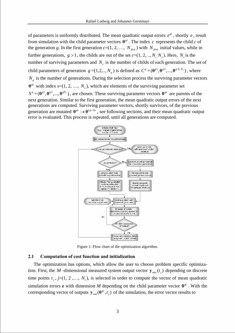
of parameters is uniformly distributed. The mean quadratic output errors gce , shortly e , result from simulation with the child parameter vectors gcθ . The index c represents the child c of the generation g. In the first generation c=(1, 2, …, firstN ) with firstN initial values, while in further generations, 1g > , the childs are out of the set c=(1, 2, .., c sN N ). Here, sN is the number of surviving parameters and cN is the number of childs of each generation. The set of

child parameters of generation g =(1,2,.., gN ) is defined as gC = 1 2( , ,..., )c sg N Ng gθ θ θ , where

gN is the number of generations. During the selection process the surviving parameter vectors gsθ with index s=(1, 2, …, sN ), which are elements of the surviving parameter set gS = 1 2( , ,..., )sgNg gθ θ θ , are chosen. These surviving parameter vectors gsθ are parents of the

next generation. Similar to the first generation, the mean quadratic output errors of the next generations are computed. Surviving parameter vectors, shortly survivors, of the previous generation are mutated ( 1)gs g c+→θ θ , see following sections, and their mean quadratic output error is evaluated. This process is repeated, until all generations are computed.

Figure 1: Flow chart of the optimization algorithm.

2.1 Computation of cost function and initialization The optimization has options, which allow the user to choose problem specific optimiza-

tion. First, the M -dimensional measured system output vector ( )mes jty depending on discrete time points jt , j=(1, 2 ,…, tN ), is selected in order to compute the vector of mean quadratic

simulation errors e with dimension M depending on the child parameter vector gcθ . With the corresponding vector of outputs ( , )gc

sim jty θ of the simulation, the error vector results to


4

( , ) ( ) ( , ).gc gcj mes j sim jt t t= −e θ y y θ (1)

At the end of the simulations with each parameter vector gcθ , the simulation errors,

are evaluated and stored. They are also called cost function values. The goal of the automatic identification algorithm is the search for the optimal parameter vector optθ such that the corre-sponding cost function value is minimal.

The dimension N of the parameter space NP ⊂ is equal to the number of user defined pa-rameters. Due to the fact, that N is infinite and the optimization process has to be finished in finite time, the components gc

iθ of the parameter vectors gcθ are limited by the user,

Furthermore, the initial population size, i.e. the number of uniform distributed parameters of the first generation of the optimization, is defined by the user. If this value is set to a very high value, the global minimum is found more likely, but the computation effort increases.

2.2 Selection process

After computation of the cost function values gce (see Eq. (2)), the surviving parameter set S is computed by selection of | |S parameter vectors gcθ with the lowest cost function values

gce . If the generation is not the first ( 1g > ), the survivors of the previous generation are also considered during the selection process.

2.3 Mutation The parameter values of the mutated parameters are located close to their parent parame-

ters, i.e. the surviving parameters. Each parameter of the first generation is normal distributed,

with new random values gcir for every component gc

iθ of each parameter vector. Related to the inverse formula of standard normal distribution, the function

is defined in order to mutate the parameters. The mutated parameters ( 1)g c+θ for the next gen-eration g+1 are computed with the user defined range reduction factor ]0,1]ξ ∈ . This factor is smaller than one in order to have decreasing influence to the distance between the child pa-rameters and the surviving parameters

2

1 1

1 [ ( , )] ,tNM

gc k gcj

k jt

e e tM N = =

= ∑∑ θ (2)

,min ,max[ , ].gci i iθ θ θ∈ (3)

,min ,max ,min( ) , [0,1],gc gc gci i i i i ir rθ θ θ θ= + − ∈ (4)

1 1 1 1sgn -log 2| | 0 12 2 2 2( ) ,

102

x x if x xs x

if x

⎧ ⎛ ⎞ ⎛ ⎞− − ≤ < ∧ < ≤⎪ ⎜ ⎟ ⎜ ⎟⎪ ⎝ ⎠ ⎝ ⎠= ⎨⎪ =⎪⎩

(5)

( 1) (g-1),max ,min( ) ( r ) .g c gs gc

i i i i isθ θ θ θ ξ+ = + − (6)


5

After evaluation of Eq. (6), each child parameter ( 1)g ciθ

+ is compared with its corresponding limits ,miniθ and ,maxiθ of the parameter space. In case of an exceeded limit, the child parameter

( 1)g ciθ

+ is set to this limit. In case of more than one minimum of the cost function in the pa-rameter space P , the optimization possibly searches near the wrong minima. To avoid this possible problem, a modified strategy of the selection process is shown in the next section.

2.4 Selection process considering multiple local minima In case of more than one multiple (local) minima of the cost function are expected during

the optimization, the surviving parameter vectors should not be placed too close together, since the optimization searches possibly near a local minima instead of the best minima of the simulation error in the parameter space P . In order to force the optimization to find several local minima at different locations in parameter space, the following strategy for the selection process is used. First, all parameters of the generation are sorted with respect to their cost functions. Then, the parameters of the simulation with lowest cost function are added to the surviving parameter set S . All sorted candidate parameters gc gC∈θ have a distance ( )gcd θ , which should be bigger than a minimal allowed distance (g-1)

min,0d ξ to all parameters in gS ,

Note, that the minimal allowed distance is decreasing every generation g, so it is possible to find minima of the cost function, which are located very close to other minima during the automatic parameter identification. The case of one dimensional parameter identification, the minimal distance factor has to be chosen

for good optimization results. In N -dimensional parameter spaces, the minimal distance fac-tor should be also chosen smaller than the diagonal of normed parameter space,

3 AUTOMATIC PARAMETER IDENTIFICATION OF BELT DRIVE In order to test the automatic parameter identification, a belt drive simulation as shown in

Fig. (2) is investigated. According to Ref. [21] with the assumption of small axial strains of the belt and a linear distribution of the displacement with respect to the initial belt lengths 0il is assumed. The displacements are defined with respect to the Lagrangian frame of reference.

2

(g-1)min,0

,max ,min

( ) min .g

s

gc gsgc i i

p S i i i

d dθ θξ

θ θ∈

⎛ ⎞⎛ ⎞−⎜ ⎟= >⎜ ⎟⎜ ⎟⎜ ⎟−⎜ ⎟⎝ ⎠⎝ ⎠∑θ (7)

min,0 1d < , (8)

2min,0 1 .

N

d N< =∑ (9)


6

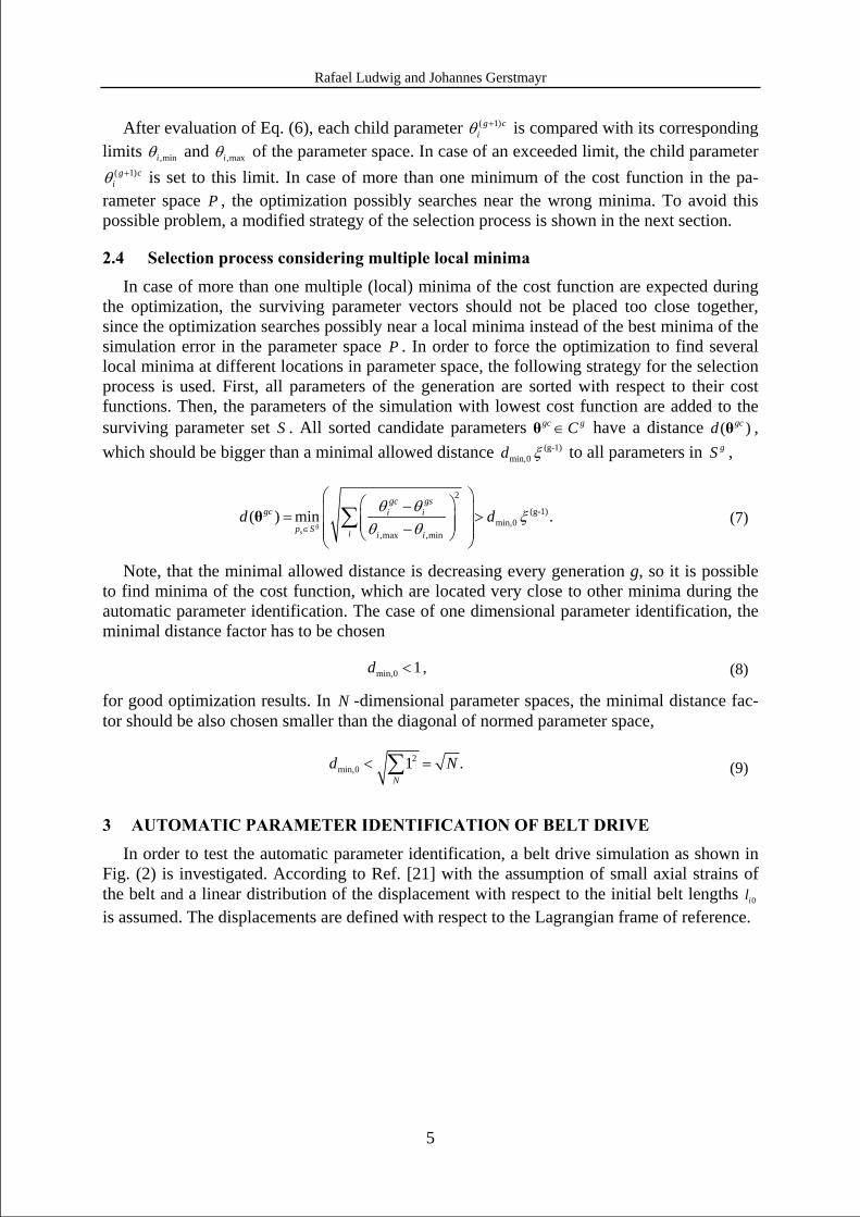
Figure 2: Belt drive model with position dependent stiffness.

The differences iuΔ between actual and initial belt lengths depend on the initial position 0( 0)x t x= = of the rail mass, the actual position x of the rail mass, the angle of the driving

gear 1ϕ and the angle of the driven gear 2ϕ are

According to Ref. [22], which deals with the experimental setup for measurement of belt parameters, the axial belt stiffnesses of each part reads

The Lagrange equations of motion of the system follow to

in which the Lagrange function

consists of the potential energy of the belt with iuΔ from Eq. (10),

and the kinetic energy of the gear inertias and the rail mass

( )( )( )

11 0

22 0

32 1 .

u r x x

u r x x

u r

ϕ

ϕ

ϕ ϕ

Δ = + −

Δ = − + −

Δ = −

(10)

0

.ii

EAkl

= (11)

1 2, { , , },j jj j

d L L Q q xdt q q

ϕ ϕ∂ ∂= + ∈

∂ ∂ (12)

L T V= − (13)

( ) ( ) ( )( )3

2 2 22 21 1 0 2 2 0 3 2 1

1

1 1 ( ) ,2 2

ii

iV k u k r x x k r x x k rϕ ϕ ϕ ϕ

=

= Δ = + − + − − − + −∑ (14)

2 2 21 1 2 2

1 1 1 .2 2 2

T m x J Jϕ ϕ= + + (15)


7

The partial derivatives of L with respect to the generalized coordinates jq are

Further terms of inertia from the derivative of the Lagrange function depending on the generalized velocities jq are

The principle of virtual work applied to the driving torque 1M and the force vector leads to the generalized forces

The equations of motion follow to

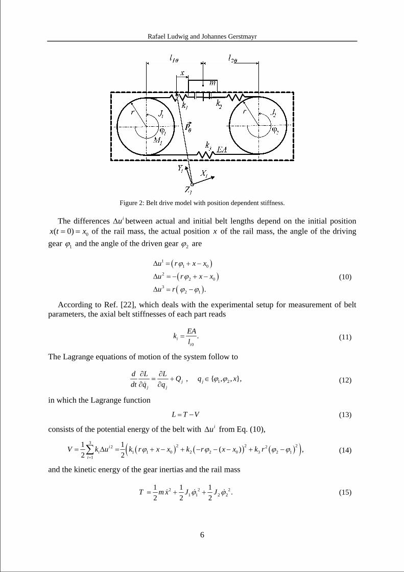
An image of the implemented model in HOTINT with the dynamic equations from Eq. (19) is shown in Fig. (3).

Figure 3: HOTINT model of belt drive - driving and driven gear are drawn to a larger scale.

In order rotate the driving gear with a prescribed angle 1dϕ , it is necessary to add a control-ler to the system. Therefore a P-controller is used to compute the driving torque

The mass and stiffness matrices of the controlled system are

( ) ( )

( ) ( )

( ) ( )

23 2 1 1 1 0

1

23 1 2 2 2 0

2

1 1 0 2 2 0 .

L k r k r r x x

L k r k r r x x

L k r x x k r x xx

ϕ ϕ ϕϕ

ϕ ϕ ϕϕ

ϕ ϕ

∂= − − + −

∂∂

= − − + −∂∂

= − + − − + −∂

(16)

1 1 2 21 2

, , .d L d L d Lmx J Jdt x dt dt

ϕ ϕϕ ϕ

∂ ∂ ∂= = =

∂ ∂ ∂ (17)

11 1 1 1 1 2

1 1 3

0

.

j jj jj j

xW M F x M q F q M F xq q

Q M Q F

ϕδ δϕ δ δ δ δϕ δϕ δ∂ ∂= + = + = + +

∂ ∂

⇒ = =

∑ ∑ (18)

( )( )3 2 1 1 1 01 1 1

2 2 2 2 0 3 2 1

2 2 0 1 1 0

( ) ( )

( ) ( )

( ) ( ) .

k r k r x xJ r M

J r k r x x k r

m x k r x x k r x x F

ϕ ϕ ϕϕ

ϕ ϕ ϕ ϕ

ϕ ϕ

− − + −= +

= − + − + −

= − + − − + − +

(19)

1 1 1( ).dM P ϕ ϕ= − (20)


8

For the simulation with nominal parameters, the following parameters are chosen

Parameter Symbol Value Unit Initial spring length of 1k 1,0l 0.1875+ 0x m Initial spring length of 2k 2,0l 0.7875- 0x m Axial stiffness EA 52 10× N Moment of inertias 1 2,J J

21 10−× 2kg m

Radius r 31 10−× m Rail mass m 0.948 kg Controller gain P 0 and 45 1Nm rad−

Table 1: Nominal parameters of belt drive simulation.

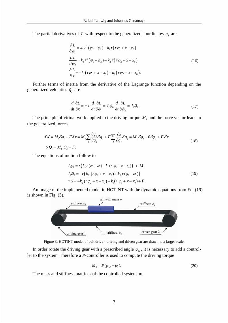
The eigenfrequencies have the following form,

With vanishing controller parameter, 0P = 1Nm rad− , 1C is also zero. 2C and 3C are posi-tive values. When the controller is turned on, the first eigenfrequency depends on P and the initial position 0x of the rail mass. The dependency on the initial position is shown in Fig. (4), where the controller gain is 45P = 1Nm rad− .

0 0.1 0.2 0.3 0.4 0.5 0.6 0.765

70

75

80

85

x0 (m)

f (H

z)

Figure 4: First eigenfrequency with proportional angle controller computed with HOTINT.

In real systems, it is often hard to get the correct controller values, therefore the controller value is identified. The axial stiffness EA of the belt is also a parameter for the identification, since the real material behaviour usually differs from the values of data sheets due to toler-ances. As measurement data, the angle 1ϕ and torque 1M of the driving gear from a reference simulation are used in order to test the identification algorithm. The reference angle 1,dϕ was prescribed in form of small steps in order to get a good excitation of the undamped system i.e. shown in Fig. (5).

1 2

2 2 21 3 3 1

2 2 23 2 2 3 2

1 2 1 2

( , , ),

-- .

diag J J m

k r k r P k r k rk r k r k r k rk r k r k k

=

⎡ ⎤+ +⎢ ⎥= +⎢ ⎥⎢ ⎥+⎣ ⎦

M

K (21)

21,2 1 3,4 2 5,6 3det( ) 0 , , .C C Cω ω ω ω− = ⇒ = ± = ± = ±K M (22)


9

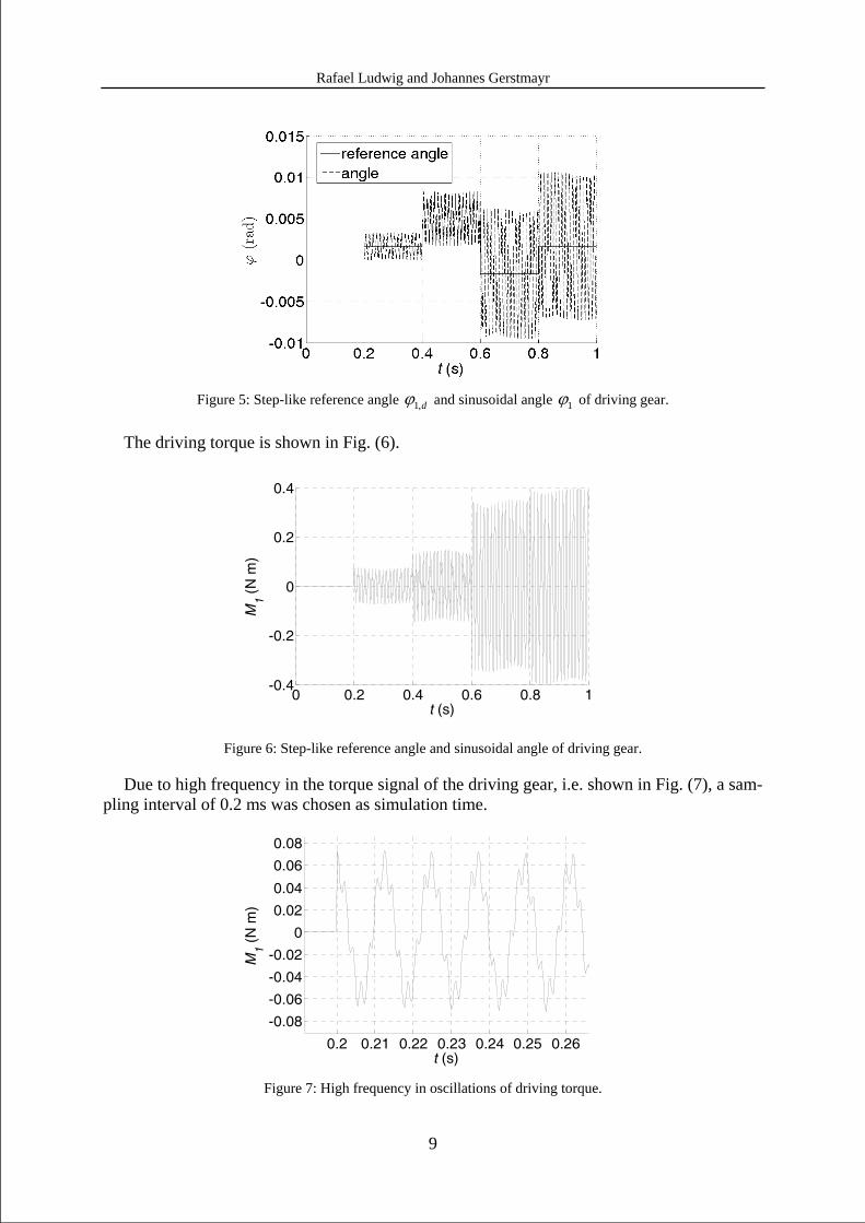
Figure 5: Step-like reference angle 1,dϕ and sinusoidal angle 1ϕ of driving gear.

The driving torque is shown in Fig. (6).

0 0.2 0.4 0.6 0.8 1-0.4

-0.2

0

0.2

0.4

t (s)

M1 (

N m

)

Figure 6: Step-like reference angle and sinusoidal angle of driving gear.

Due to high frequency in the torque signal of the driving gear, i.e. shown in Fig. (7), a sam-pling interval of 0.2 ms was chosen as simulation time.

0.2 0.21 0.22 0.23 0.24 0.25 0.26

-0.08

-0.06

-0.04

-0.02

0

0.02

0.04

0.06

0.08

t (s)

M1 (

N m

)

Figure 7: High frequency in oscillations of driving torque.


10

In following, the influence of the number of surviving parameters is shown. The parame-ters are searched in the intervals 5 5[1.5 10 ,2.5 10 ] NEA∈ × × and -1[30,60] Nm radP∈ .

Identification parameter Value Initial population size 1000 Cardinality | |S of surviving parameter set 8 and 20 Number of Children of each survivor 8 Number of generations g 12 Range reduction factor ξ 0.5 Minimal distance min,0d 0 and 0.5

Table 2: Settings of identification algorithm.

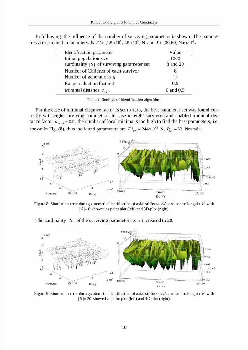
For the case of minimal distance factor is set to zero, the best parameter set was found cor-rectly with eight surviving parameters. In case of eight survivors and enabled minimal dis-tance factor min,0 0.5d = , the number of local minima is too high to find the best parameters, i.e. shown in Fig. (8), thus the found parameters are 3244 10optEA = × N, 53optP = -1Nm rad .

Figure 8: Simulation error during automatic identification of axial stiffness EA and controller gain P with

| | 8S = showed as point plot (left) and 3D-plot (right).

The cardinality | |S of the surviving parameter set is increased to 20.

Figure 9: Simulation error during automatic identification of axial stiffness EA and controller gain P with

| | 20S = showed as point plot (left) and 3D-plot (right).


11

In this case, the optimized parameters 200056optEA = N and 45.0145optP = -1Nm rad are very close to the nominal parameters. The simulation error and the tested parameters during the optimization are shown in Fig. (9). Remarkable are the high number of local minima with re-spect to the axial stiffness EA . The big influence of the axial stiffness to a phase shift of the gear angle is reason for this behavior. Nevertheless, with a sufficient number of initial values, the original values can be retrieved easily.

4 AUTOMATIC IDENTIFICATION OF PARAMETERS OF GENERIC ROBOT The generic robot is described in Ref. [18] and Ref. [19]. As short summary, the generic

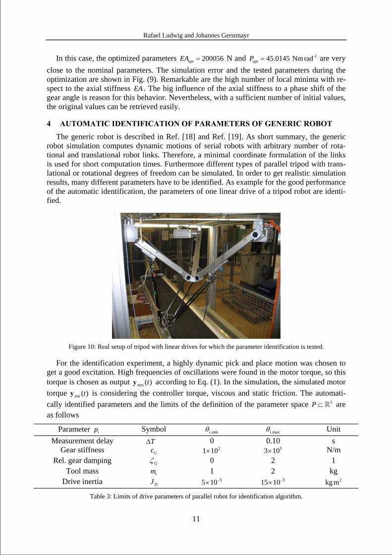
robot simulation computes dynamic motions of serial robots with arbitrary number of rota-tional and translational robot links. Therefore, a minimal coordinate formulation of the links is used for short computation times. Furthermore different types of parallel tripod with trans-lational or rotational degrees of freedom can be simulated. In order to get realistic simulation results, many different parameters have to be identified. As example for the good performance of the automatic identification, the parameters of one linear drive of a tripod robot are identi-fied.

Figure 10: Real setup of tripod with linear drives for which the parameter identification is tested.

For the identification experiment, a highly dynamic pick and place motion was chosen to get a good excitation. High frequencies of oscillations were found in the motor torque, so this torque is chosen as output ( )mes ty according to Eq. (1). In the simulation, the simulated motor torque ( )sim ty is considering the controller torque, viscous and static friction. The automati-cally identified parameters and the limits of the definition of the parameter space 5P ⊂ are as follows

Parameter ip Symbol ,miniθ ,maxiθ Unit Measurement delay TΔ 0 0.10 s

Gear stiffness Gc 21 10×

53 10× N/m Rel. gear damping Gζ 0 2 1

Tool mass tm 1 2 kg Drive inertia DJ

55 10−× 515 10−×

2kg m Table 3: Limits of drive parameters of parallel robot for identification algorithm.


12

The time delay TΔ denotes the transfer times of the motor torque values into a file. In the simulation, the electric torque of the controller circuit is subtracted by static and viscous fric-tion terms. This torque is multiplied with the gear factor and a link side equivalent force result and acts on the rail additionally to the gravitation force. Further, a multiplication of the drive inertia with the square of the gear factor leads to equivalent mass em of the moment of inertia of the motor results. The rail mass railm is well known from the data sheet. Between the rail mass and the equivalent mass from drive inertia DJ is a spring damper element with stiff-ness Gc and damping Gd representing the mechanical gear effects. For better physical inter-pretation, the relative damping factor Gξ is identified. The damping of the spring damper element is

A constraint equation with Lagrange parameter keeps the distance between the rail and the tool mass constant. For the automatic identification algorithm, the following parameters are used

Identification parameter Value Initial population size 1024 Cardinality | |S of surviving parameter set 8 Number of Children of each survivor 8 Number of generations g 12 Range reduction factor ξ 0.5 Minimal distance min,0d 0 and 0.5

Table 4: Settings of identification algorithm.

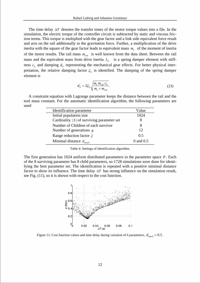
The first generation has 1024 uniform distributed parameters in the parameter space P . Each of the 8 surviving parameter has 8 child parameters, so 1728 simulations were done for identi-fying the best parameter set. The identification is repeated with a positive minimal distance factor to show its influence. The time delay TΔ has strong influence on the simulation result, see Fig. (11), so it is shown with respect to the cost function.

Figure 11: Cost function values and time delay during variation of 6 parameters, min,0 0.5d = .

2 .e rail GG G

e rail

m m cdm m

ξ=+

(23)


13

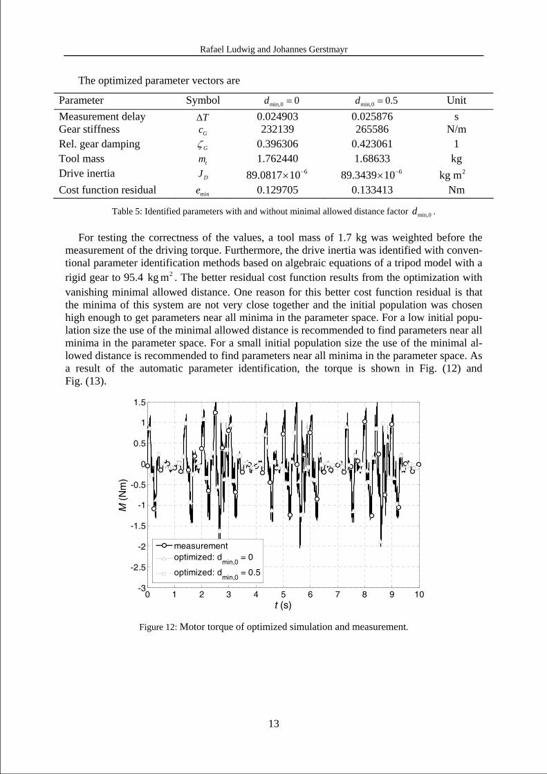
The optimized parameter vectors are

Parameter Symbol min,0 0d = min,0 0.5d = Unit Measurement delay TΔ 0.024903 0.025876 s Gear stiffness Gc 232139 265586 N/m Rel. gear damping Gζ 0.396306 0.423061 1 Tool mass tm 1.762440 1.68633 kg Drive inertia DJ 89.0817 610−× 89.3439 610−× 2kg m Cost function residual mine 0.129705 0.133413 Nm

Table 5: Identified parameters with and without minimal allowed distance factor min,0d .

For testing the correctness of the values, a tool mass of 1.7 kg was weighted before the measurement of the driving torque. Furthermore, the drive inertia was identified with conven-tional parameter identification methods based on algebraic equations of a tripod model with a rigid gear to 95.4 2kg m . The better residual cost function results from the optimization with vanishing minimal allowed distance. One reason for this better cost function residual is that the minima of this system are not very close together and the initial population was chosen high enough to get parameters near all minima in the parameter space. For a low initial popu-lation size the use of the minimal allowed distance is recommended to find parameters near all minima in the parameter space. For a small initial population size the use of the minimal al-lowed distance is recommended to find parameters near all minima in the parameter space. As a result of the automatic parameter identification, the torque is shown in Fig. (12) and Fig. (13).

0 1 2 3 4 5 6 7 8 9 10-3

-2.5

-2

-1.5

-1

-0.5

0

0.5

1

1.5

t (s)

M (

Nm

)

measurementoptimized: d

min,0 = 0

optimized: dmin,0

= 0.5

Figure 12: Motor torque of optimized simulation and measurement.


14

7.5 8 8.5 9-3

-2.5

-2

-1.5

-1

-0.5

0

0.5

1

1.5

( )

M (

Nm

)

measurementoptimized: d

min,0 = 0

optimized: dmin,0

= 0.5

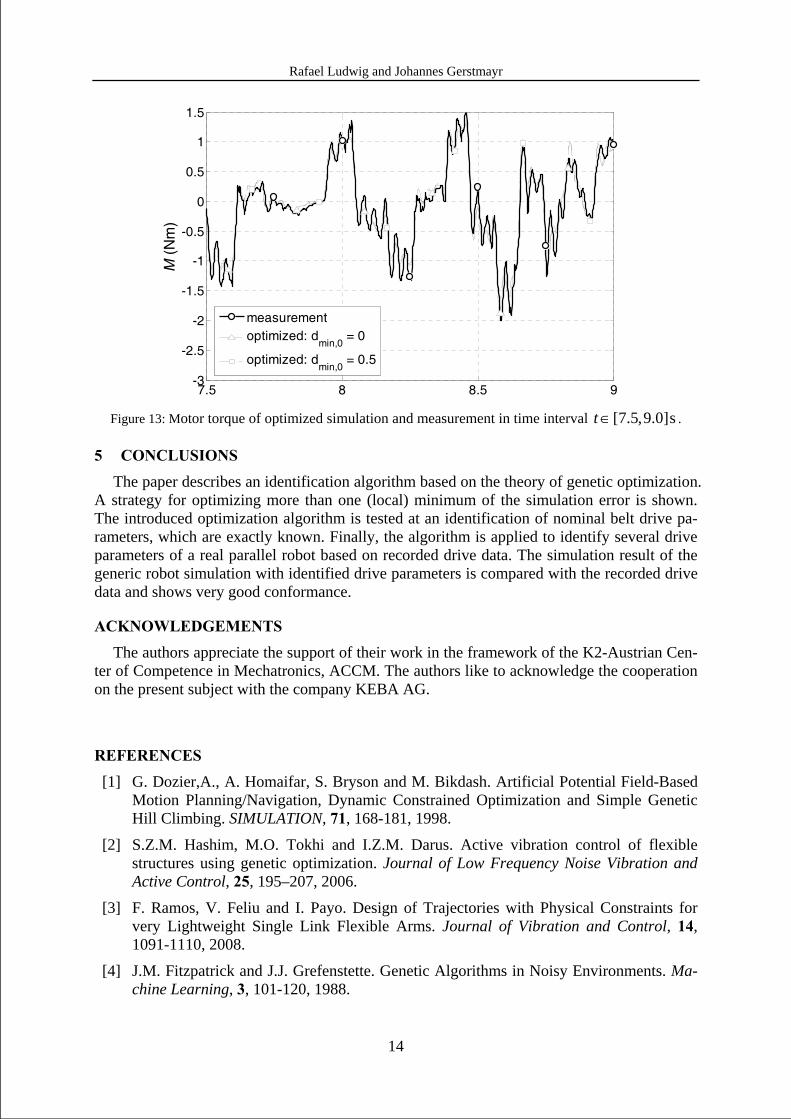
Figure 13: Motor torque of optimized simulation and measurement in time interval [7.5,9.0]st∈ .

5 CONCLUSIONS The paper describes an identification algorithm based on the theory of genetic optimization.

A strategy for optimizing more than one (local) minimum of the simulation error is shown. The introduced optimization algorithm is tested at an identification of nominal belt drive pa-rameters, which are exactly known. Finally, the algorithm is applied to identify several drive parameters of a real parallel robot based on recorded drive data. The simulation result of the generic robot simulation with identified drive parameters is compared with the recorded drive data and shows very good conformance.

ACKNOWLEDGEMENTS The authors appreciate the support of their work in the framework of the K2-Austrian Cen-

ter of Competence in Mechatronics, ACCM. The authors like to acknowledge the cooperation on the present subject with the company KEBA AG.

REFERENCES [1] G. Dozier,A., A. Homaifar, S. Bryson and M. Bikdash. Artificial Potential Field-Based

Motion Planning/Navigation, Dynamic Constrained Optimization and Simple Genetic Hill Climbing. SIMULATION, 71, 168-181, 1998.

[2] S.Z.M. Hashim, M.O. Tokhi and I.Z.M. Darus. Active vibration control of flexible structures using genetic optimization. Journal of Low Frequency Noise Vibration and Active Control, 25, 195–207, 2006.

[3] F. Ramos, V. Feliu and I. Payo. Design of Trajectories with Physical Constraints for very Lightweight Single Link Flexible Arms. Journal of Vibration and Control, 14, 1091-1110, 2008.

[4] J.M. Fitzpatrick and J.J. Grefenstette. Genetic Algorithms in Noisy Environments. Ma-chine Learning, 3, 101-120, 1988.


15

[5] M.R. Heinen and F.S. Osório. Applying Genetic Algorithms to Control Gait of Physi-cally Based Simulated Robots. IEEE Congress on Evolutionary Computation, 2006.

[6] J.L. Martínez, A. Mandow, J. Morales, S. Pedraza and A. García-Cerezo. Approximat-ing Kinematics for Tracked Mobile Robots. The International Journal of Robotics Re-search, 24, 867-878, 2005.

[7] X. Xiaomin, S. Qing, Z. Ling and Z. Bin. Parameter Estimation and its Sensitivity Analysis of the MR Damper Hysteresis Model Using a Modified Genetic Algorithm. Journal of Intelligent Material Systems and Structures, 20, 2089-2100, 2009.

[8] M.S. De Queiroz. An Active Identification Method of Rotor Unbalance Parameters. Journal of Vibration and Control, 15, 1365–1374, 2009.

[9] T.K. Teng, J.S. Shieh and C.S. Chen. Genetic algorithms applied in online autotuning PID parameters of a liquid-level control system. Transactions of the Institute of Meas-urement and Control, 5, 433–450, 2003.

[10] A. Zakharov and S. Halasz. PARAMETER IDENTIFICATION OF A ROBOT ARM USING GENETIC ALGORITHMS. PERIODICA POLYTECHNICA SER. EL. ENG, 45, 195–209, 2001.

[11] A. Arakawa and K. Miyata. A Simultaneous Optimization Algorithm for Determining Both Mechanical-System and Controller Parameters for Positioning Control Mecha-nisms. 4th International Workshop on Advanced Motion Control Proceedings, 1996.

[12] L. Ljung. System Identification – Theory for the User – Second Edition. Prentice-Hall, N.J., 1999.

[13] A.J. Fairweather, M.P.Foster and D.A. Stone. VRLA BATTERY PARAMETER IDENTIFICATION USING PSEUDO RANDOM BINARY SEQUENCES (PBRS). 5th IET International Conference on Power Electronics, Machines and Drives, 2010.

[14] J. Gerstmayr, HOTINT. A C++ Environment for the simulation of multibody dynamics systems and finite elements. Proceedings of the Multibody Dynamics Eccomas The-matic Conference, 1-20, 2009.

[15] A.A. Shabana. Dynamics of Multibody Systems - Second Edition. Cambridge university press, USA, 1998.

[16] H. Bremer and F. Pfeiffer. Elastische Mehrkörpersysteme. B. G. Teubner, Stuttgart, 1992.

[17] M. Fliess, C. Join and H. Sira-Ramírez. Non-linear estimation is easy. Int. J. Modelling Identification and Control 4, 1, 2008.

[18] R. Ludwig, J. Gerstmayr, C. Augdopler and C. Mittermayer. Realistic Robot Simulation with Flexible Components. Proceedings of the 5th International Conference on Compu-tational Intelligence, Robotics and Autonomous Systems (CIRAS), 187-192, 2008.

[19] R. Ludwig, J. Gerstmayr, C. Augdopler and C. Mittermayer. Flexible Robot with Clear-ance. 4th Proceedings of the European Conference on Structural Control, 2, 511-518, 2008.

[20] M. Fliess and H. Sira-Ramírez. AN ALGEBRAIC FRAMEWORK FOR LINEAR IDENTIFICATION. ESAIM: Control, Optimisation and Calculus of Variations, 9, 151-168, 2003.


16

[21] F. Ziegler, Technische Mechanik der festen und flüssigen Körper, Springer Verlag, Wien, 1998.

[22] G. Cepon, L. Manin, Introduction of damping into the flexible multibody belt-drive model: A numerical and experimental investigation, Journal of Sound and Vibration, 324, 2009.

automatic parameter identification for generic robot …€¦ · automatic parameter identification...

Documents