automatic detection of trypanosomes on the blood stream
TRANSCRIPT
FACULDADE DE ENGENHARIA DA UNIVERSIDADE DO PORTO
Automatic Detection of Trypanosomeson the Blood Stream
José Rui Neto Faria
Mestrado Integrado em Engenharia Informática e Computação
Supervisor at FEUP: Luís Filipe Pinto de Almeida Teixeira
Supervisor at FhP: Fábio Filipe Costa Pinho
July 22, 2016


Automatic Detection of Trypanosomes on the BloodStream
José Rui Neto Faria
Mestrado Integrado em Engenharia Informática e Computação
Approved in oral examination by the committee:
Chair: João Carlos Pascoal FariaExternal Examiner: Pedro Manuel Henriques da Cunha Abreu
Supervisor: Luís Filipe Pinto de Almeida TeixeiraJuly 22, 2016


Abstract
Despite the major advancements in Medical Science of the XXI century, there are still dangerousdiseases spread worldwide. Two of them chagas disease and the sleeping sickness are potentiallylife-threatening illnesses caused by the protozoan parasites: Trypanosoma cruzi (T. cruzi) andTrypanosoma brucei (T. brucei) respectively. These diseases are mainly found in Latin Americaand Africa being transmitted to humans and animals by small insects like triatomine bugs andtsetse flies either by bite or contact with their faeces, killing a high number of people by latediagnostic.
The chagas disease has two phases, the initial (acute) phase lasts about two months after infec-tion, in this phase a high number of parasites circulate in the blood stream, but in most cases thesymptoms are absent or mild. In the second phase, chronic phase, the parasites are hidden mainlyin the heart and digestive muscles, in later years the infection can lead to sudden death or heartfailure caused by progressive destruction of the heart muscle and digestive system.
The sleeping sickness also has two phases, the initial phase, last from some weeks to oneor two years depending of the sub-species of the T.brucei parasite, in this phase a high numberof parasites circulate in the blood stream, and some patients suffer from fever and aches. Inthe second phase, the parasite reaches the nervous system causing mental deterioration and otherneurological problems leading to the death of the patient.
The objective of this work was to create a mobile solution that can help detect both the diseasesin the initial stages by detecting the trypanossomes parasites. With this application, the user takes aphoto of a thin blood smear sample of a patient using an adapter that attaches the mobile device toa microscope, then the image is segmented in order to separate the components of the blood fromits background. Later, the application will try to confirm if the parasites segmented are the correctones, informing the user if the donor of the blood is infected. With this, it becomes possible tomake the detection of the diseases in countries where the health services are poorly developed andpeople do not have good access to it. This mobile application is fast and reliable due to its analysissensibility of 97.37% and its short execution time of approximately 32 seconds on a high-endandroid device
i

ii

Resumo
Hoje em dia existem várias doenças consideradas perigosas. Duas delas, a doença de chagas ea do sono, são mortais e causadas pelos parasitas protozoários: Trypanosoma cruzi (T. cruzi) eTrypanosoma brucei (T. brucei) respetivamente. Essas doenças aparecem geralmente na AméricaLatina e África sendo transmitidas a seres humanos e animais por pequenos insetos como o tri-atomine e tsetse através de mordidas. Estas doenças causam elevado número de mortes devido adiagnósticos tardios.
A doença de chagas tem duas fases, a inicial(aguda), que dura até duas semanas depois dainfeção, sendo que nesta fase um grande grupo de parasitas circula na corrente sanguínea e ossintomas são quase inexistentes tornando o seu diagnóstico atempado difícil. Na segunda fase,a fase crónica, os parasitas desaparecem da corrente sanguínea e movem-se para o coração emúsculos digestivos levando à morte por falha desses mesmos orgãos.
A doença do sono também tem duas fases, a fase inicial,que pode durar desde uma semana adois anos dependendo da sub-espécie de T.brucei, nesta fase existe um grande número de parasitasna corrente sanguínea e alguns pacientes sofrem de dores de cabeça e febre. Na segunda fase oparasita chega ao sistema nervoso causando a deterioração da saúde mental do paciente levando àsua morte.
Este projeto disponibiliza uma solução móvel que permite detetar ambas as doenças nos seusestados iniciais encontrando os respetivos parasitas e permitindo o seu tratamento. Com estaaplicação, o utilizador tira fotos de uma amostra de sangue pertencente a um paciente, usando ummicroscópio com adaptador ou microstage. A foto será segmentada de modo a separar o fundo daimagem do resto dos componentes seguindo-se a identificação dos parasitas. Com isto torna-sepossível a deteção destas doenças em países menos desenvolvidos onde os serviços de saúde e oacesso aos mesmos não são garantidos. Esta solução é rápida e eficaz devido à sensibilidade de97.37% na sua análise e à sua curta duração de 32 segundos num dispositivo android consideradohigh-end.
iii

iv

Acknowledgements
I would like to thank my thesis supervisor professor Luís Filipe Pinto de Almeida Teixeira ofFaculdade de Engenharia do Porto, its door was always open whenever I ran into problem and thediscussions I had with him made me see the problem in a different light.
I would also like to thank the engineer Fábio Filipe Costa Pinho, my responsible in FraunhoferAICOS, his guidance and insight helped my to organize my project.
I would also like to acknowledge Maria João Medeiros de Vasconcelos and Luis Filipe CaeiroMargalho Guerra Rosado, engineers in Fraunhofer AICOS for helping me with the managementof resources and for having the availability to hear my problems and to help me find the solutions.
In last I want to thank Rui Neves and Simão Felgueiras, colleagues of mine that were alsodoing their thesis in Fraunhofer AICOS, and by whom I learned many things in order to improvemy project.
José Rui Neto Faria
v

vi

” Okay, well, sometimes science is more art than science, Morty.”
Rick Sanchez
vii

viii

Contents
1 Introduction 11.1 Motivation . . . . . . . . . . . . . . . . . . . . . . . . . . . . . . . . . . . . . . 11.2 Project and objectives . . . . . . . . . . . . . . . . . . . . . . . . . . . . . . . . 11.3 Structure of the dissertation . . . . . . . . . . . . . . . . . . . . . . . . . . . . . 2
2 Background 32.1 Chagas disease . . . . . . . . . . . . . . . . . . . . . . . . . . . . . . . . . . . 3
2.1.1 Transmission . . . . . . . . . . . . . . . . . . . . . . . . . . . . . . . . 32.1.2 Stages . . . . . . . . . . . . . . . . . . . . . . . . . . . . . . . . . . . . 32.1.3 Diagnosis . . . . . . . . . . . . . . . . . . . . . . . . . . . . . . . . . . 42.1.4 Treatment . . . . . . . . . . . . . . . . . . . . . . . . . . . . . . . . . . 42.1.5 The parasite . . . . . . . . . . . . . . . . . . . . . . . . . . . . . . . . . 4
2.2 Sleeping sickness . . . . . . . . . . . . . . . . . . . . . . . . . . . . . . . . . . 62.2.1 Transmission . . . . . . . . . . . . . . . . . . . . . . . . . . . . . . . . 62.2.2 Stages . . . . . . . . . . . . . . . . . . . . . . . . . . . . . . . . . . . . 62.2.3 Diagnosis . . . . . . . . . . . . . . . . . . . . . . . . . . . . . . . . . . 72.2.4 Treatment . . . . . . . . . . . . . . . . . . . . . . . . . . . . . . . . . . 72.2.5 The parasite . . . . . . . . . . . . . . . . . . . . . . . . . . . . . . . . . 7
2.3 Trypanossoma cruzi vs Trypanossoma brucei . . . . . . . . . . . . . . . . . . . 9
3 Literature review 113.1 Image recognition . . . . . . . . . . . . . . . . . . . . . . . . . . . . . . . . . . 11
3.1.1 Preprocessing . . . . . . . . . . . . . . . . . . . . . . . . . . . . . . . . 113.1.2 Segmentation . . . . . . . . . . . . . . . . . . . . . . . . . . . . . . . . 143.1.3 Feature extraction . . . . . . . . . . . . . . . . . . . . . . . . . . . . . . 193.1.4 Classification . . . . . . . . . . . . . . . . . . . . . . . . . . . . . . . . 21
3.2 Technology review . . . . . . . . . . . . . . . . . . . . . . . . . . . . . . . . . 233.2.1 Computer vision . . . . . . . . . . . . . . . . . . . . . . . . . . . . . . 233.2.2 Mobile Operating System . . . . . . . . . . . . . . . . . . . . . . . . . 243.2.3 Image acquisition . . . . . . . . . . . . . . . . . . . . . . . . . . . . . . 253.2.4 Summary . . . . . . . . . . . . . . . . . . . . . . . . . . . . . . . . . . 26
3.3 Similar projects . . . . . . . . . . . . . . . . . . . . . . . . . . . . . . . . . . . 263.3.1 Malaria Scope . . . . . . . . . . . . . . . . . . . . . . . . . . . . . . . 263.3.2 Athelas . . . . . . . . . . . . . . . . . . . . . . . . . . . . . . . . . . . 263.3.3 Columbia Engineering mobile application . . . . . . . . . . . . . . . . . 27
3.4 Conclusion . . . . . . . . . . . . . . . . . . . . . . . . . . . . . . . . . . . . . 27
ix

CONTENTS
4 Implementation 294.1 Image Dataset . . . . . . . . . . . . . . . . . . . . . . . . . . . . . . . . . . . . 29
4.1.1 Image Dataset Requirements . . . . . . . . . . . . . . . . . . . . . . . . 294.1.2 Image acquisition . . . . . . . . . . . . . . . . . . . . . . . . . . . . . . 29
4.2 Preprocessing . . . . . . . . . . . . . . . . . . . . . . . . . . . . . . . . . . . . 294.2.1 Image cropping . . . . . . . . . . . . . . . . . . . . . . . . . . . . . . . 30
4.3 Segmentation . . . . . . . . . . . . . . . . . . . . . . . . . . . . . . . . . . . . 304.3.1 Determining the aperture diameter . . . . . . . . . . . . . . . . . . . . . 314.3.2 Color segmentation using LAB color space . . . . . . . . . . . . . . . . 314.3.3 Area threshold . . . . . . . . . . . . . . . . . . . . . . . . . . . . . . . 33
4.4 Features . . . . . . . . . . . . . . . . . . . . . . . . . . . . . . . . . . . . . . . 334.5 Classification . . . . . . . . . . . . . . . . . . . . . . . . . . . . . . . . . . . . 35
4.5.1 Classification training . . . . . . . . . . . . . . . . . . . . . . . . . . . 354.5.2 Classification testing . . . . . . . . . . . . . . . . . . . . . . . . . . . . 374.5.3 Results and decision . . . . . . . . . . . . . . . . . . . . . . . . . . . . 39
4.6 Mobile application . . . . . . . . . . . . . . . . . . . . . . . . . . . . . . . . . 394.6.1 Application overview . . . . . . . . . . . . . . . . . . . . . . . . . . . . 404.6.2 Application requirements . . . . . . . . . . . . . . . . . . . . . . . . . . 434.6.3 Image processing module integration . . . . . . . . . . . . . . . . . . . 43
5 Validation of the mobile application 455.1 Execution time . . . . . . . . . . . . . . . . . . . . . . . . . . . . . . . . . . . 455.2 Results . . . . . . . . . . . . . . . . . . . . . . . . . . . . . . . . . . . . . . . . 48
6 Conclusions and future work 49
References 51
x

List of Figures
2.1 Triatomine bugs [CHA] . . . . . . . . . . . . . . . . . . . . . . . . . . . . . . . 32.2 The phases of trypanosoma cruzi. . . . . . . . . . . . . . . . . . . . . . . . . . 52.3 Life cycle of T.Cruzi [CDCb] . . . . . . . . . . . . . . . . . . . . . . . . . . . . 52.4 Tsetse fly [SLE] . . . . . . . . . . . . . . . . . . . . . . . . . . . . . . . . . . . 62.5 T. brucei trypomastigote in thin blood smears stained with Giemsa[CDCa]. . . . 82.6 Life cycle of T.Brucei [SLE] . . . . . . . . . . . . . . . . . . . . . . . . . . . . 82.7 Trypomastigotes comparation. . . . . . . . . . . . . . . . . . . . . . . . . . . . 9
3.1 Gaussian blur . . . . . . . . . . . . . . . . . . . . . . . . . . . . . . . . . . . . 123.2 Representation of RGB figure . . . . . . . . . . . . . . . . . . . . . . . . . . . 153.3 Channel subtraction process . . . . . . . . . . . . . . . . . . . . . . . . . . . . 163.4 Area threshold . . . . . . . . . . . . . . . . . . . . . . . . . . . . . . . . . . . . 173.5 Split and merge process . . . . . . . . . . . . . . . . . . . . . . . . . . . . . . . 173.6 Example of figure gradient 1 . . . . . . . . . . . . . . . . . . . . . . . . . . . . 183.7 RGB color histogram . . . . . . . . . . . . . . . . . . . . . . . . . . . . . . . . 203.8 KNN process . . . . . . . . . . . . . . . . . . . . . . . . . . . . . . . . . . . . 213.9 SVM Result . . . . . . . . . . . . . . . . . . . . . . . . . . . . . . . . . . . . . 223.10 Simple decision tree example . . . . . . . . . . . . . . . . . . . . . . . . . . . . 233.11 Microscope with skylight . . . . . . . . . . . . . . . . . . . . . . . . . . . . . . 253.12 Fraunhofer microstage . . . . . . . . . . . . . . . . . . . . . . . . . . . . . . . 26
4.1 Crop process . . . . . . . . . . . . . . . . . . . . . . . . . . . . . . . . . . . . 304.2 Lab channels of the figure . . . . . . . . . . . . . . . . . . . . . . . . . . . . . . 314.3 Result from Color segmentation . . . . . . . . . . . . . . . . . . . . . . . . . . 324.4 Result from Area segmentation . . . . . . . . . . . . . . . . . . . . . . . . . . . 334.5 Resulting figures of the marking process . . . . . . . . . . . . . . . . . . . . . . 364.6 Resulting figures of the marking process . . . . . . . . . . . . . . . . . . . . . . 364.7 Learning phase of the program . . . . . . . . . . . . . . . . . . . . . . . . . . . 374.8 Testing phase of the program . . . . . . . . . . . . . . . . . . . . . . . . . . . . 384.9 Simple application database diagram . . . . . . . . . . . . . . . . . . . . . . . . 404.10 Android application activities figures . . . . . . . . . . . . . . . . . . . . . . . . 414.11 Android application activities figures . . . . . . . . . . . . . . . . . . . . . . . . 424.12 Android application activities figures . . . . . . . . . . . . . . . . . . . . . . . . 42
5.1 Image example . . . . . . . . . . . . . . . . . . . . . . . . . . . . . . . . . . . 48
xi

LIST OF FIGURES
xii

List of Tables
3.1 Different blur types . . . . . . . . . . . . . . . . . . . . . . . . . . . . . . . . . 123.2 Different types of color spaces . . . . . . . . . . . . . . . . . . . . . . . . . . . 14
4.1 TCGFE features . . . . . . . . . . . . . . . . . . . . . . . . . . . . . . . . . . . 344.2 Classification algorithms . . . . . . . . . . . . . . . . . . . . . . . . . . . . . . 354.3 Results of classification algorithms . . . . . . . . . . . . . . . . . . . . . . . . . 39
5.1 Process duration on a computer . . . . . . . . . . . . . . . . . . . . . . . . . . . 465.2 Process duration on an Asus Zenfone 2 . . . . . . . . . . . . . . . . . . . . . . . 465.3 Process duration on a galaxy nexus . . . . . . . . . . . . . . . . . . . . . . . . . 475.4 Results of the program . . . . . . . . . . . . . . . . . . . . . . . . . . . . . . . 48
xiii

LIST OF TABLES
xiv

Abbreviations
CPU central process unitKNN K-nearest neighboursOpenCV Open Source Computer Vision LibraryRAM Random Access MemoryRGB Red,Green,BlueROI Region of interestSVM Support vector machineT. b. gambiense Trypanosoma brucei gambienseT. b. rhodesiense Trypanosoma brucei rhodesienseT. brucei Trypanosoma bruceiT. cruzi Trypanosoma cruzi
xv


Chapter 1
Introduction
1.1 Motivation
Trypanosomes infect a variety of hosts and are responsible for many diseases that affected humans
and animals alike, two of the most dangerous diseases to humans chagas disease and sleeping
sickness, are caused by T.cruzi and T.brucei two sub-species of Trypanosomes.
Chagas disease is a potentially life-threatening illness, being found mainly in Latin America.
Per year there are 41,200 new cases of T cruzi infection, 14,400 infants are born with congenital
Chagas disease and 12,000 die from it[eme]. The cost of treatment for Chagas disease remains
substantial. In Colombia alone, the annual cost of medical care for all patients with the disease
was estimated to be about US$ 267 million in 2008 [CHA].Spraying insecticide to control the
bugs responsible for the transmission of it would cost nearly US$ 5 million annually.
The sleeping sickness cases are generally prevalent in Africa, in 1998 40 000 cases were
reported, but more than 300 000 cases were undiagnosed and untreated [SLE]. A more recent
epidemic happened in Africa and the prevalence of the disease reached 50% in several villages
in Angola, South Sudan and the Democratic Republic of the Congo. In the last years the cases
of the disease decreased to 9878 cases in 2009 and 3796 in 2014 due to control efforts.The esti-
mated number of actual cases is below 20 000 and the estimated population at risk is 65 million
people[SLE].
This project aims to help the reduction of these numbers by giving a portable option for de-
tecting both diseases in the early stages and making the treatment possible.
1.2 Project and objectives
The objective of this work is to create an android application that detects if someone is infected
with the early stages of the chagas disease or the sleeping sickness by analyzing a picture of a blood
sample retrieved from a possibly infected person and detecting the parasite responsible for the
diseases: Trypanosoma cruzi or Trypanosoma brucei respectively. For that first a good computer
1
Introduction
vision methodology must be created using as support the contextualization of the problem and the
searched state of the art.
This application should run in a variety of android devices and have a good performance
depending of the mobile system hardware like battery, processor and memory. The work of the
application can be reduced to 3 steps: acquire a picture either by taking a photo of the blood
sample using an adapter to attach the device to a microscope or by loading an image from the
gallery, analyze it using methods from computer vision and show the result to the user.
1.3 Structure of the dissertation
The present document has five other chapters:
Chapter 2: Gives background about the diseases and the related parasites in order to help the
reader understanding better the processes that will be used in the application and how it will work;
Chapter 3: Makes a revision and evaluation of the work done in the area which this project is
inserted, this includes the existent computer vision algorithms, similar mobile applications in the
market and conclusions about the collected information;
Chapter 4: Explains the used computer vision methodology, all its steps and how it was used
in an android application
Chapter 5: Tests a group of images and its results are discussed.
Chapter 6: Concludes the dissertation and points out future.
2

Chapter 2
Background
2.1 Chagas disease
2.1.1 Transmission
Chagas disease, also known as American trypanosomiasis, is a potentially life-threatening illness
caused by the Trypanosoma cruzi (T. cruzi). This parasite is mainly transmitted by contact with
faeces/urine of infected blood-sucking triatomine bugs. These bugs are active at night and live in
the cracks of the poorly constructed houses. They usually bite exposed areas of skin and defecate
close to them. When the person smears the faeces into the bite, the eyes, the mouth or into any skin
break the parasite enters the body and the disease starts [CHA]. The T.cruzi can also be transmitted
by consumption of food contaminated with it, blood transfusion from infected donors, passage
from an infected mother to her newborn, organ transplant from infected donors and laboratory
accidents[CDCb].
Figure 2.1: Triatomine bugs [CHA]
2.1.2 Stages
There are two phases of Chagas disease: the acute phase and the chronic phase. The first phase,
lasts from the first weeks to the first months of the infection. It is usually symptom free or with
3

Background
mild symptoms associated, generally mistaken for other diseases. These symptoms can include
fever, fatigue, body aches, headache, rash, loss of appetite, diarrhea, and vomiting. The most
recognized marker of acute Chagas disease is called Romaña’s sign, which includes swelling of
the eyelids on the side of the face near the bite wound or where the bug faeces were deposited or
accidentally rubbed into the eye. It his in this phase that a high number of parasite circulate in
the blood, being the phase when it is easier to detect a disease from a blood sample and where the
application of the project will be used[eme].
The chronic phase is when the most symptoms are felt, as the parasites stop to circulate in the
blood and hide themselves mainly in the heart and digestive muscles of the infected person [CHA]
feeding on their cells, this causes a progressive destruction of the muscles, leading to sudden death
or heart failure of its carrier[eme].
2.1.3 Diagnosis
The chagas disease can be detected by observation of the parasite T.cruzi in a thin blood smear,
this method can only be used in the acute phase of the disease because as said in chapter 2.1.2
the parasites in the chronic phase are no longer circulating on the bloodstream of the infected
person[CDCb]. In the chronic phase serologic tests are used to detect the disease if symptoms of
it are detected in the patient. This method tests the presence of a specific antibodies to T.cruzi and
is not as well developed as the one used in the acute phase [eme].
2.1.4 Treatment
The treatment of the chagas disease is different depending on the phase of the illness the patient is
in. During the acute phase and in the beginning of the chronic phase of the disease when the patient
symptoms do not exist or are mild an anti-parasitic treatment is used, this treatment has as objective
to eliminate the parasites in the blood stream by using benznidazole and nifurtimox, which have
a reduced effect as the patient’s time without diagnosis and respective treatment increases. This
treatment is not possible in pregnant women or by people with kidney or liver failure. Nifurtimox is
also contra-indicated for people with a background of neurological or psychiatric disorders.[CHA]
The symptomatic treatment is used in the chronic phase,when the anti-parasitic treatment
should not be given, helping people who have cardiac or intestinal problems caused by the chagas
disease, this solution will not cure the infected person but will improve life quality[eme].
2.1.5 The parasite
The protozoan parasite, Trypanosoma cruzi, causes Chagas disease and it will be detected by the
application so that it can be possible to know if the patient is infected. This parasite lives part of
its life in the blood and/or tissues of the infected hosts and the rest of it in the digestive tracts of
the infecting bugs.
In its life cycle the Trypanosoma cruzi can change between many forms like trypomastig-
otes (figure 2.2a), amastigotes (figure 2.2b) and epimastigotes (figure 2.2c), to better explain this
4

Background
(a) T. cruzi trypomastigote inthin blood smears stained withGiemsa[CDCb].
(b) Trypanosoma cruzi amastig-otes in heart tissue[CDCb].
(c) Trypanosoma cruzi epimastig-ote from culture[CDCb].
Figure 2.2: The phases of trypanosoma cruzi.
changes, their purpose and when they happen we need to talk about the life cycle of the parasite.
The Trypanosoma cruzi life cycle can be divided in 2 major phases: the human stages and the
Triatomine bug stages.
Figure 2.3: Life cycle of T.Cruzi [CDCb]
The first stage starts with the bite of the Triatomine bug, when this insect takes a blood meal
and releases trypomastigotes in its faeces near the bite wound, later the parasite either by the
wound or by other skin break infects the host. Once inside of the wound the parasite invades the
nearer cells and differentiates into intracellular amastigotes. In this phase the parasite can multiply
by binary fission using cells infected tissue, after multiplying in the cell the parasite transforms
into trypomastigotes and goes to the blood stream, then when finding a suitable cell it transforms
5
Background
again in amastigotes, this last two phases are repeated until the infected person is cured or dead.
The second major phase happens in the Triatomine bug, starting with this insect getting in-
fected with trypomastigotes after biting an animal or human infected with the parasite, in this
stage the T.cruzi evolves in the digestive system of the insect. In the midgut the trypomastigote
evolves to epimastigote and multiplies and differentiates, in the hindgut the epimastigote goes
back to trypomastigotes[CDCb].
The two major phases described previously are cyclic and are represented in the figure 2.3
with the color blue to the human stages and the color red to the Triatomine bug stages.
2.2 Sleeping sickness
2.2.1 Transmission
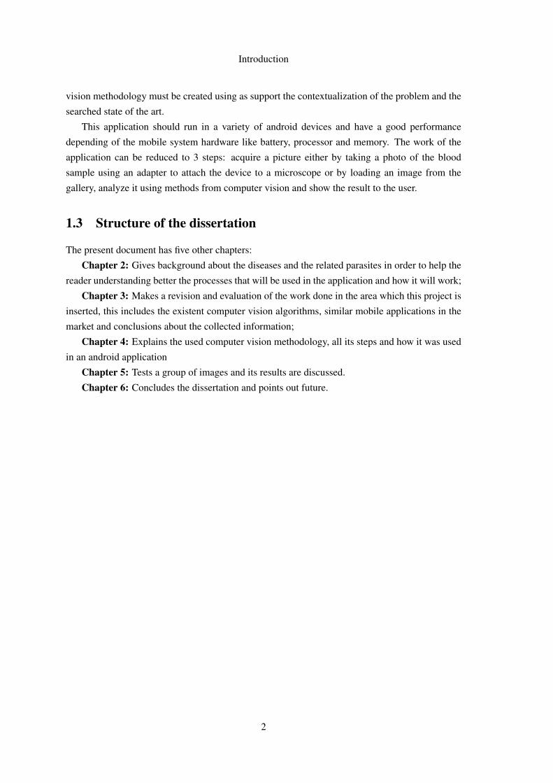
Sleeping sickness also known as African Trypanosomiasis, is a potentially life-threatening illness
caused by the Trypanosoma brucei (T. brucei). This parasite is mainly transmitted by bite of
infected blood-sucking tsetse flies. Tsetse flies are mainly found in the sub-Saharan Africa though
only some species transmit the disease, the regions where the majority of the cases occur are
places that depend of the agriculture, fishing, animal husbandry or hunting. The disease develops
in areas ranging from a single village to an entire region. Within an infected area, the intensity of
the disease can vary from region to the other[SLE].
Figure 2.4: Tsetse fly [SLE]
2.2.2 Stages
The sleeping sickness has two phases, in the first stage, like the chagas disease, the parasite is
found in big quantities in the peripheral circulation of the infected patient, the patient suffers from
symptoms like fever, headache, muscle and joint aches[CDCa]. The duration of this phase depends
of the sub-specie of T.brucei that infected the patient:
6

Background
• T. b. rhodesiense: this infection progresses rapidly, most patients develop fever, headache,
muscle and joint aches, and enlarged lymph nodes within 1-2 weeks of the infective bite.
After a few weeks the parasite invades the nervous system and the second stage starts.
• T. b. gambiense: progresses more slowly than the T.b. rhodesiense and the symptoms are
weaker. Infected people may have intermittent fevers, headaches, muscle and joint aches.
Usually the first stage lasts one to two years.
The second stages leads to the death of the patient, in this phase the parasite is found in the central
nervous system and starts causing problems like personality changes, daytime sleepiness with
night-time sleep disturbance, and progressive confusion. The time of death of the patient also
depends of the sub-species, if the patient is infected with T. b. rhodesiense the subject will die
in few months after the infection otherwise if infected with T. b. gambiense the death happens in
about 3 years but is preceded by progressive destruction of the nervous system[CDCa].
2.2.3 Diagnosis
The sleeping sickness can be detected by observation of the parasite T.brucei in a thin blood
smear, generally the load of the sub-specie T. b. rhodesiense infection is higher than the level in
the T. b. gambiense infection[CDCa]. Both parasites can also be found in the lymph node fluid,
generally the T. b. gambiense its easier to be detected by observation of the node fluid. All patients
diagnosed with the disease must have their cerebrospinal fluid examined to determine the stage of
the infection and the respective treatment.
2.2.4 Treatment
The treatment of the sleeping sickness is different depending on the phase of the disease the patient
is in. The drugs used in the first stage of the disease are safer and easier to administer than those
from the second stage. Meaning the earlier the disease is identified the better the prospect of cure.
In the first stage of the disease two different drugs are used for the treatment: Pentamidine
and Suramin, the first is used for the treatment of T.b. gambiense and the second for the treatment
of the T.b. rhodiense. In the second phase Melarsoprol, Eflornithine and Nifurtimox are used for
the treatment. The Melarsoprol is used to treat both of sub-species of the T.brucei parasite, the
Eflornithine and Nifurtimox only work against T.b. gambiense, furthermore the last one has only
been tested in animals.[SLE]
2.2.5 The parasite
The protozoan parasite, Trypanosoma brucei, causes sleeping sickness, and it will be detected by
the application so that it can be possible to know if the blood is infected. This parasite lives part
of its life in the blood and/or tissues of the infected hosts and the rest of it in the digestive tracts of
the infecting bugs.
7

Background
Figure 2.5: T. brucei trypomastigote in thin blood smears stained with Giemsa[CDCa].
In its life cycle the Trypanosoma brucei can change between many forms like trypomastig-
otes(figure 2.2a) and epimastigotes, to better explain this changes, their purpose and when they
happen we need to talk about the life cycle of the parasite. The Trypanosoma brucei life cycle can
be divided in 2 major phases: the human stages and the Tsetse flies stages.
Figure 2.6: Life cycle of T.Brucei [SLE]
The first phase starts with the bite of the tsetse fly, when this insect takes a blood meal and
releases trypomastigotes to the bloodstream from there they are carried to other sites throughout
the body, reaching other body fluids (e.g., lymph, spinal fluid) and replicating by binary fission.
Later a tsetse fly can become infected by taking a blood meal from an infected person or animal.
8

Background
In the Tsetse fly the parasite reaches the midgut after infecting it, transforming in to procyclic
trypomastigotes that can multiply by binary fission. Later they transform into epimastigotes and
reach the fly’s salivary glands and continue multiplication by binary fission.
The two major phases described previously are cyclic and are represented in the image 2.6
with the color blue for the human stages and the color red for the Triatomine bug stages.
2.3 Trypanossoma cruzi vs Trypanossoma brucei
The program will try to detect the parasites in the patient bloodstream, as seen in the section 2.1.5
and 2.2.5 both the T.cruzi and the T.brucei will be detected in the trypomastigote stage.
(a) T. cruzi trypomastigote in thin bloodsmears stained with Giemsa[CHA].
(b) T. brucei trypomastigote in thin bloodsmears stained with Giemsa[SLE].
Figure 2.7: Trypomastigotes comparation.
As seen in the figures 2.7a and 2.7b both parasites have similar color and shape in the blood
samples stained with giemsa. The biggest difference between them is the size of the kinoplast as
seen in the figures. Another difference between them is that the T.brucei can only be found in the
trypomastigote stage in the human body and the T.cruzi can be also found in the amastigote form
in various tissues.
9

Background
10
Chapter 3
Literature review
3.1 Image recognition
In this section the algorithms associated with an object recognition problem will be shown and
explained being grouped among the four phases of the problem: Preprocessing, segmentation,
feature extraction and classification.
3.1.1 Preprocessing
Preprocessing is the first step of the figure recognition problem where the objective is to prepare
and improve the overall quality of the figure. For many people this step is discarded since it can
distort or change the raw data of the figure. However an intelligent use of it can provide benefits
and solve problems that ultimately lead to a better performance of the program [Kri14].
In the preprocessing generally the methods aim to change the properties of the pixels in the
figure like: the color and brightness in order to solve problems like pixel noise and too much
brightness difference. The preprocessing phase can also be used to change the figure in order to
remove information that will not be needed in the later stages of the program.
3.1.1.1 Blur
Generally figure blurring is not considered a positive property in an figure because of the loss of
information that is associated with it, but there are cases where this type of operation can have
positive result if applied in a correct and controlled way [Kri14].
The blur operations (also known as smoothing) are algorithms applied to an figure to blur
and eliminate different pixel noises from it, like per example: salt and pepper noise, where white
and black pixels appear alone in the figure creating problems in the later stages of the analyze by
obstructing important information. These algorithms blur the figure by creating a window(with
odd size) which will pass every pixel in the figure convolving its matrix with a defined kernel
depending of the blur subtype, the next table shows different blurs and their respective kernels:
11

Literature review
Table 3.1: Different blur types
Type characteristics
Mean filter After convolving the content of the window with the kernel the
value of the pixel is the mean value of the group pixels contained
in the window
Median filter After convolving the content of the window with the kernel the
value of the pixel is the median value of the group pixels con-
tained in the window
Gaussian filter In this blur the window is convoluted with a kernel created by a
Gaussian function, the result is the value of the central pixel of
the window
Kuwahara filter This blur divides the window in 4 sub-windows and calculates the
mean value of each, in the end the value of the central pixel is the
mean value of that region that has the smallest variance.
Nagao-Matsuyama filter This blur uses a 5x5 window divided in 9 sub-windows to cal-
culate the value of its central pixel, its value is the mean of the
sub-window with the lowest variance
These types of algorithms are greatly affected by the size of the window, generally the biggest
the window size the blurriest the result is (figure 3.1), this property is one of the most important
properties of the process.
(a) Original figure 1 (b) Window size 3
(c) Window size 7 (d) Window size 15
Figure 3.1: Gaussian blur
12

Literature review
3.1.1.2 Image resize
This is one of the most simple preprocessing methods, its objective is not to improve the results
of the posterior operations but to make the overall program faster. This method generally by
reducing the resolution or size of the figure reduces the quantity of pixels to be analyzed, this
makes algorithms that have to get and modify the information of all the pixels in the figure faster
due to their reduced number. The image resize can be a double-edged sword due to the result
of the operation, an figure that has been reduced a lot will lose important information and will
deteriorate the results of the segmentation,feature extraction and classification phases.
3.1.1.3 Image crop
The objective of this preprocessing method is the same as the image resize but is applied in a
different way. With image crop the size of the figure will be changed not due to a universal resize
but a cut of regions of the figure that will not be necessary for the rest of the program. The problem
of this method is that can not be easily applied to all figure due to the fact that, in some figures, the
region of interest is hard to discover and consequently the area to be cut too. The big advantage
compared to the figure resize is the fact that, as said before, the pixels are not changed and the
discarded information is not necessary avoiding problems in later stages of the project.
3.1.1.4 Modification of color space
This type of method tries to correct or enhance the color information of an figure, making the
later steps of the overall object recognition process faster and more reliable. For that generally
the original figure color space is changed to another color space that can be either a different
representation of the same colors with different properties or a totally new color space created by
the user using information present in the figure[?].
In Table 3.2 some of the most well known color spaces are identified and characterized.
1This figure is taken from http://imgbuddy.com/blood-smear-staining.asp
13

Literature review
Table 3.2: Different types of color spaces
color space characteristics
RGB This is one of most common color spaces, each color is repre-
sented by the sum of the red,green and blue colors
HSV In this color space each color is represented by the hue, saturation,
and value(or brightness)
GRAY In this color space every color is represented by a gray-scale color,
generally is used to simplify the figure
LAB In this color space every color is represented by lightness and a
and b coordinate for the color-opponent dimension
CMY It represents the 3 links used in color printing: cyan, magenta and
yellow
CMYK It represents the 4 links used in color printing: cyan, magenta,
yellow and black
As said before the user can also create their own color space this can be reached by either
changing the components from an existent color space, or by using many different channels to
create an figure, making the identification of the different components of the figure easier. An
example of a created color space could be an gray-scale figure where the pixel value is calculated
by subtracting the RGB channel Red to the sum of the Blue and Green channels, this would create
figure where only the components that have a red color component inferior to the sum of the other
two would be shown, and the brighter components would be the ones where the red component is
minor compared to the other two.
This step can also be used as an intermediate step in the color segmentation algorithms being
applied generally to a copy of the figure to allow the selection of component existent in the figure.
3.1.2 Segmentation
The segmentation is the process of dividing the figure into multiple smaller segments. The ob-
jective is to simplify and change the representation of an figure into something easier to analyze.
In our current problem that would be dividing the background, foreground and its elements that
represent the many constituents of the blood smear, later they can be identified individually in the
classification phase using the features extracted. Segmentation algorithms are generally based in
two image properties: intensity values discontinuity and similarity. The first spots different seg-
ments by detecting the abrupt changes between them like the color and brightness change of a
group of pixels. The second category finds different segments by encountering similar groups of
pixels.[AaKK10]
14

Literature review
3.1.2.1 Using the difference between color channels
This method uses the difference in the color channels of the image color space to remove the
majority of the background and some elements of the foreground that are not the desired object.
In the first step of this segmentation algorithm the figure is separated in different sub-figures, which
one representing the presence of a channel in the original figure, the darker the pixel the weaker
is the value of the represented channel in that pixel[SMUCBLRP13]. This step can be applied to
many different color spaces like the RGB, HSV, LAB and CMYK, for explanation proposes the
example below will be in a RGB color space.
(a) Original figure 2 (b) Red channel
(c) Green channel (d) Blue channel
Figure 3.2: Representation of RGB figure
In Figure 3.2, the parasite positioned in the center of the figure is mainly red and blue the
green channel is weaker and the intensity of the background in the 3 channels is almost the same.
So, by taking advantage of these differences, and computing the difference between the blue and
green channels some information of the figure can be retrieved. The result of this operation is
the figure 3.3a where the background is dark and the parasite and some unwanted subsets are
lighter[SMUCBLRP13]. To improve the result of the previous operation a color threshold follow-
ing the formula below should be applied.
f (n) =
white if | Blue-Green |> T
black otherwise
2This figure is taken from http://imgbuddy.com/blood-smear-staining.asp
15
Literature review
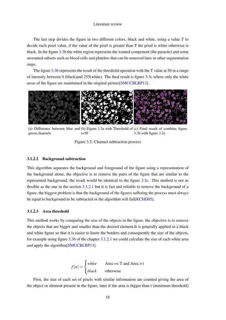
The last step divides the figure in two different colors, black and white, using a value T to
decide each pixel value, if the value of the pixel is greater than T the pixel is white otherwise is
black. In the figure 3.3b the white region represents the wanted component (the parasite) and some
unwanted subsets such as blood cells and platelets that can be removed later in other segmentation
steps.
The figure 3.3b represents the result of the threshold operation with the T value at 50 in a range
of intensity between 0 (black)and 255(white). The final result is figure 3.3c where only the white
areas of the figure are maintained in the original picture[SMUCBLRP13].
(a) Difference between blue andgreen channels
(b) Figure 3.3a with Threshold oft=50
(c) Final result of combine figure3.3b with figure 3.2a
Figure 3.3: Channel subtraction process
3.1.2.2 Background subtraction
This algorithm separates the background and foreground of the figure using a representation of
the background alone, the objective is to remove the parts of the figure that are similar to the
represented background, the result would be identical to the figure 3.3c. This method is not as
flexible as the one in the section 3.1.2.1 but it is fast and reliable to remove the background of a
figure, the biggest problem is that the background of the figures suffering the process must always
be equal to background to be subtracted or the algorithm will fail[KCHD05].
3.1.2.3 Area threshold
This method works by comparing the size of the objects in the figure, the objective is to remove
the objects that are bigger and smaller than the desired element.It is generally applied in a black
and white figure so that it is easier to know the borders and consequently the size of the objects,
for example using figure 3.3b of the chapter 3.1.2.1 we could calculate the size of each white area
and apply the algorithm[SMUCBLRP13].
f (n) =
white Area =< T and Area > t
black otherwise
First, the size of each set of pixels with similar information are counted giving the area of
the object or element present in the figure, later if the area is bigger than t (minimum threshold)
16
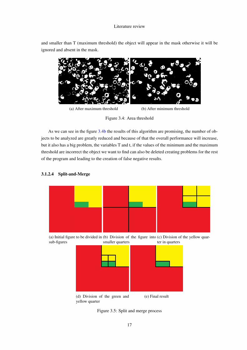
Literature review
and smaller than T (maximum threshold) the object will appear in the mask otherwise it will be
ignored and absent in the mask.
(a) After maximum threshold (b) After minimum threshold
Figure 3.4: Area threshold
As we can see in the figure 3.4b the results of this algorithm are promising, the number of ob-
jects to be analyzed are greatly reduced and because of that the overall performance will increase,
but it also has a big problem, the variables T and t, if the values of the minimum and the maximum
threshold are incorrect the object we want to find can also be deleted creating problems for the rest
of the program and leading to the creation of false negative results.
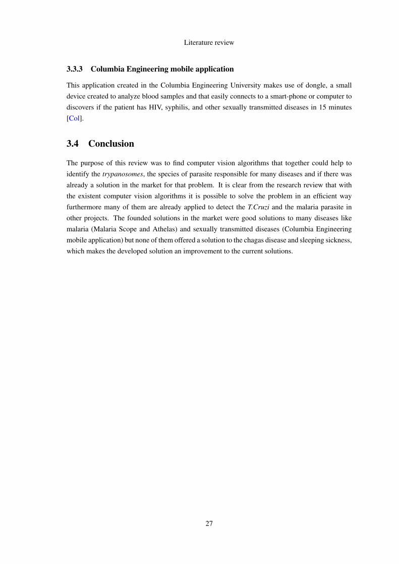
3.1.2.4 Split-and-Merge
(a) Initial figure to be divided insub-figures
(b) Division of the figure intosmaller quarters
(c) Division of the yellow quar-ter in quarters
(d) Division of the green andyellow quarter
(e) Final result
Figure 3.5: Split and merge process
17

Literature review
This is a simple method that divides the figure in many different sub-figures. This algorithm starts
by dividing the initial figure in four different quarters (figure 3.5b), after that the program will test
them with the predicate. In the predicate the color present in the quarters is tested, if the quarter
has a big variation of color inside of it, then it is divided again in more quarters (figure 3.5d),
otherwise the division does not occur and instead of it if the neighbours quarters have a similar
color are merged(figure 3.5e). This phase is repeated until every segment as a similar color inside
of it and division is not possible[KG08].
In the end the result of this algorithm is an figure divided by its color variance, changing if the
color space was altered in the preprocessing phase.
3.1.2.5 Watershed
Watershed is a group of algorithms that separate the figure in sub-figures by detecting the color
difference between areas, all of them start in the same way, first the gray figure is converted to
an intensity gradient magnitude of an figure, this gradient will look like a topographic surface,
and will have maximums and minimums created by clearer and darker intensities[CHYL09]. The
watersheds algorithms are divided in:
• flooding algorithm:This algorithm finds the separations of the sub-figures by "flooding" the
minimum points of the intensity gradient, when different water sources meet a separation of
the figures is created, the resulting group of separations are all the lines where the figures is
divided.
• rainfall algorithm:in this algorithm "raindrops" are placed in each pixel of the figure, the
raindrop will flow to a local minimum using gradient descent, all the pixels with the same
minimum are part of the same sub-figure.
Figure 3.6: Example of figure gradient 3
The watershed algorithm has problems with noise, conducting to over-segmentation of areas,
to reduce that risk a blur algorithm(chapter 3.1.1.1) should be used before the operation[CHYL09].3This figure is taken from http://photos1.blogger.com/blogger/3551/3073/320/Reliefimg.jpg
18

Literature review
3.1.2.6 Mean-shift
The mean-shift algorithm is an advanced and versatile technique for clustering based segmentation
that divides the figure in sub-figures modeling feature vectors associated with each pixel(color,position)
with a density function. After the creation of a 2d space of the points with the density function,
the algorithm for each pixel will:
• create a search window:This window can be rectangular or circular and includes many
different pixels, and it will be positioned in the figure.
• calculate the mass center of the window:in this stage using the density function of the
pixels the figure will calculate the mass center of them.
• move window to mass center:after the last step the center of the window is positioned in
the mass center moving the window to a denser group.
• return to second step: this will happen until the center of the window is the same as the
mass center.
The objective is to associate the many pixels to a denser area, and with them create a sub-
figure. This algorithm is considered efficient and robust but its results depends on the density
function used[Ngu].
3.1.3 Feature extraction
Feature extraction is one of the most important step to resolving successfully an object recognition
problem, from the resulting features of its appliance to the classification systems (chapter 3.1.4)
will be trained and if the wrong type of features are chosen the classification will, consequently,
fail in the identification of the parasite creating false positive and negative results.
3.1.3.1 Using color histogram
A color histogram is a representation of the quantity of pixels of each color present in the figure,
it can be built for many color representations, like HSV, RGB and YCM. To help the explanation
the RGB color space will be used, to use this type of histogram, first the figure must be divided
in the 3 channels and its intensity sub-histograms must be extracted, the final results represent the
distribution of the color in the figure. For example, looking at figure 3.7 we come to the conclusion
that the figure has not many pixels with strong blue and green channels.
This type of features are good for identification of an object that has always similar color
distribution otherwise if the object can appear with many different colors, or is identified in places
where the lightning changes its color value then the use of this features causes incorrect results
and must be avoided [SB91].
19

Literature review
Figure 3.7: RGB color histogram
3.1.3.2 Hu moments
Hu moments are features derivated from algebraic combinations of the first 3 orders of normal-
ized central moments, describing, characterizing, and quantifying the shape of an object in an
figure[Li10]. Hu Moments are normally extracted from the silhouette or outline of an object in
an figure, extracting a shape feature vector (i.e. a list of numbers) to represent the shape of the
object[Li10]. Later that feature vector will be compared to others to find if the objects are the
same. In the end this type of features fails to identify objects whose shape can change in different
figures creating problems in the classification phase.
3.1.3.3 Color correlogram
The color correlogram (henceforth correlogram) can be seen as an extended colour histogram, it
expresses how the spatial correlation of pairs of colors changes with distance. Informally a color
correlogram of and figure is a table where each entry represents the probability of finding a pixel
of color j at a distance k from a pixel of color i in the figure[JKM+94].
This type of features is robust, tolerating changes in the viewing positions, changes in back-
ground,partial occlusions, camera zoom and are a good solution for problems of figure recogni-
tion, but has the same problem as Hu Moments, objects which the shape is not constant can not be
correctly identified[JKM+94].
3.1.3.4 SIFT
Scale-invariant feature transform is an algorithm that detects and extracts the local features of an
figure, that features are scale, rotation and brightness invariant[Low99]. The SIFT algorithm can
be divided in many stages:
• Detection: In this stage the algorithm identifies the interest points of the figure, for that,
features like corners and edges of the figure are separated and detected. First Lowe’s method
transforms the figure in a matrix of feature vectors, is this part that makes the features
invariant.Then key locations are found by the difference of gaussians founding the best
local features.
• Description:After the last step the features are extracted, indexed and saved.
• Matching: In the last stage of the algorithm, the saved points are compared to the points of
the figure. To improve the matching of points the euclidean distance can be used.
20

Literature review
3.1.4 Classification
In this phase the program, using the information retrieved by the segmentation and feature extrac-
tion phase learns what an object is, and later can identify it.
3.1.4.1 K-nearest neighbours
In object recognition, the k-Nearest Neighbours algorithm is a machine learning method used for
classification of objects. In the KNN algorithm the objects are evaluated by comparing with other
objects that were learned by it, this algorithm is also known as a lazy algorithm[K-n].
The algorithm is divided in two parts: learning and classification, in the first one a group of figures
and their respective features (see chapter 3.1.3) are given to the algorithm and their classification,
with that information the algorithm will create a representation of the needed groups in a 2d fea-
ture space (figure 3.8a, where the green triangles and the red circles represent different groups).
In the second stage, classification, an figure is evaluated by the algorithm using the model estab-
lished previously, in this phase the features of the evaluated figure is compared to the others that
were given in the previous step and then the figure is placed on the 2d space, from there the algo-
rithm will find the K closest figures (figure 3.8b, where blue quad is the new figure), in the end the
algorithm chooses the class of the figure by seeing the classes of the closest points and going with
the majority (figure 3.8b).
(a) End of learning stage KNN (b) Beginning of classificationstage KNN,k=3
(c) End of classification stage
Figure 3.8: KNN process
This algorithm is robust and works well with big quantities of data being a good solution to
the problem of classifying a big quantity of different objects its biggest problem is the definition
of the parameter K and its high computational cost[K-n].
3.1.4.2 Support Vector Machine
The support vector machine is a supervised learning model that classifies an figure as being one
of two classes.This algorithm receives a group of figures, maps them in a 2D space using their
features and then tries to find a function that translates the general rule of the figures (figure 3.9),
21

Literature review
creating a line that separates both classes, new examples are then mapped into that same space and
their class identified[CV95].
Figure 3.9: SVM Result
This algorithm is good against problems of two classes, one vs one or one vs all, being its
biggest problem that the function can have over-fitting, that means some objects are classified
incorrectly [CV95].
3.1.4.3 Naive Bayes classifier
The bayes classifier is a learning probabilistic classifier that follows the Bayes theorem to classify
figures, that means that the answer given by it is an probability of the object being of a certain
class. For that the class is trained following the formula:
P(Cn|Fx) = P(Cn)∗P(Fx|Cn)P(Fx)
Where P(Cn|Fx) is the probability of the object being of a certain class n if feature x is detected,
the P(Fx|Cn) is the inverse, and the P(Cn) and P(Fx) are the probabilities of being of class n and
having feature x. P(Fx) is calculated by dividing the number of times the feature x appear in the
figures for the total of figures and P(Cn) is defined in priori of the calculations.
But what happens when multiple features are detected? We have to calculate the probability
for an object to be part of a class taking in account all the features.One way to simplify the problem
is using the naive bayes classifier[Leu07]. The naive bayes classifier finds which class the object is
more probable of being part by simplifying the formula above to one single variable, P(Fx|Cn), this
happens because P(Cn) and P(Fx) have always the same value being desregarded in the calculation,
so to calculate the probability of P(F1,F2,F3,...,Fx|Cn), where all F is all the features:
P(F1,F2,F3, ...,Fx|Cn) = P(F1|Cn)∗P(F2|Cn)∗P(F3|Cn)∗ ...∗P(Fx|Cn)
The biggest the result the biggest the probability that the object is part of a class, this result
can only be used as comparison with the results from other classes[Leu07].
22

Literature review
3.1.4.4 Decision tree
A decision tree is a classification algorithm that uses a tree graph model to make decisions about
the class of the object.In this algorithm, generally, the nodes represents a result and each branch a
decision or feature (figure 3.10).
Figure 3.10: Simple decision tree example
This graph can be also read as If <condition1>,<condition2>,...,and <conditionN> then <re-
sult> making it easier to understand than others classification methods.
3.2 Technology review
This thesis has as objective the creation of a mobile application that uses an figure processing
methodology that can detect and count trypanosomes. Thus, some technological aspects must be
considered in the development stage of this project, which will be described in the next sections.
3.2.1 Computer vision
3.2.1.1 OpenCV
OpenCV is an open source machine learning and computer vision library created to facilitate and
accelerate the use of machine perception and figure processing algorithms in computer vision
programs. This library has more than 2500 optimized algorithms, that can be used to detect and
recognize faces, identify objects, classify human actions in videos, track camera movements, track
moving objects and many more.
OpenCV has C++, C, Python, Java and MATLAB interfaces and supports Windows, Linux,
Android and Mac OS. Making one of the most used libraries.[ABO]
23

Literature review
3.2.1.2 FastCV
FastCV is a computer vision library aimed to the android mobile platform, used to create real-
time computer vision applications. FastCV is optimized for use in ARM architectures, usu-
ally associated with mobile devices improving the overall performance and speed of the created
applications.[Fas]
3.2.2 Mobile Operating System
The figure processing methodology aims to be used in a mobile operating system. These operating
systems control all the features of the mobile devices like GPS, Wi-fi, camera, mobile communi-
cation system and user interface.In this thesis the context of the camera features are particularly
important due to the fact that the camera will take the pictures to be analyzed. In this sub section
the 3 most popular mobile operating systems will be described.
3.2.2.1 Android
Android is an operating system currently developed by Google based on the Linux kernel used
by mobile devices like mobile-phones,tablets and smart-watches. This is the mobile operating
system with the most market share being the best-selling mobile OS since 2013.In September
2015, Android had 1.4 billion monthly active users.
The Android primary app store is know as Google Play, with over one million applications
and billions of downloads.
The popularity of the system is mostly due to its open source code and licensing, being used by
many different companies together with their proprietary software, Its open nature also attracted
a large community of developers and enthusiasts to use the open-source code as a foundation for
community-driven projects.
The main programming language used to developed native application in android is the android
java language.
3.2.2.2 iOS
This mobile operating system is developed by Apple Inc., is used exclusively by Apple devices and
it was unveiled when the iPhone was launched in 2007. This operating system is more controlled,
monitored and restricted than the android operating system. Moreover, it is updated annually.
The iOS is the second most popular mobile operating system in the world by sales after An-
droid. Its only used by apple devices like the Iphone and Ipad.Its primary app store is Apple’s App
Store with more than 1.4 million iOS applications and more than 100 billion downloads.
The main programming language used to developed native application in the iOS is the Objective-
C language.
24

Literature review
3.2.2.3 Windows Phone
This is the most recent operating system of the three presented in this sub-section, it was created
by Microsoft and it is mostly used in recent nokia mobile devices.
The windows phone has a small market share due to its late entry into the smart-phone mar-
ket.However this system is recovering the market difference thanks to their development tools like
Visual Studio and developer community.
Generally the applications of this system are written in C# ,visual basic.NET or C++ and can
be used in computer and mobile systems alike.
3.2.3 Image acquisition
In this subsection some methods to acquired figure from blood samples with big amplifications
will be shown.
3.2.3.1 Skylight
The skylight is an adapter that allows the use of a mobile phone to take pictures of samples by
aligning the camera lens of the device with the microscope.[iPh]
Figure 3.11: Microscope with skylight
3.2.3.2 Fraunhofer microstage
This is a prototype created in Fraunhofer AICOS, the objective is to connect a mobile phone to
the device and take pictures of the blood samples either by using a manual ui in the mobile phone
or automatically using focus metrics. This devices gets all the commands and energy from the
mobile phone using a micro usb cable.[Mic]
25

Literature review
Figure 3.12: Fraunhofer microstage
3.2.4 Summary
This master thesis aims to create a methodology that detects and counts trypanosomes for mobile
devices. Because of time constraints the prototype should be created and optimized for one mobile
platform, being the android chosen because of its large market share and subsequent wider use.
To program the computer vision methodology the OpenCV library will be used due to the fact
that fastCV is still limited and does not have machine learning functions. The OpenCV library also
supports multi-platform development making possible to create initially the methodology on the
computer and test it. Later, when the program is ready it can be passed to the android application
by using JNI (a technology that converts c++ code to android Java) and OpenCVSDK.
3.3 Similar projects
In this section different mobile applications that detect diseases will be demonstrated.
3.3.1 Malaria Scope
This mobile Android application created by Fraunhofer in cooperation with the infectious diseases
department of the Instituto Nacional de Saúde Dr. Ricardo Jorge, aims to create a mobile solution
to pre-diagnosis of Malaria in medically underserved areas. The project also includes a magnifi-
cation gadget that can be connected to the smart-phone and provide the necessary magnification
capability replacing the microscope for a more portable solution.[Mal].
3.3.2 Athelas
Created in a hackathon, this mobile application detects malaria by analyzing blood samples pic-
tures taken by mobile phones using low-cost lens attachment that amplifies it, the objective is
to provide faster and cheaper alternatives to existing diagnostic procedures saving lives in places
where the health services are poor or non existent. [Ath]
26
Literature review
3.3.3 Columbia Engineering mobile application
This application created in the Columbia Engineering University makes use of dongle, a small
device created to analyze blood samples and that easily connects to a smart-phone or computer to
discovers if the patient has HIV, syphilis, and other sexually transmitted diseases in 15 minutes
[Col].
3.4 Conclusion
The purpose of this review was to find computer vision algorithms that together could help to
identify the trypanosomes, the species of parasite responsible for many diseases and if there was
already a solution in the market for that problem. It is clear from the research review that with
the existent computer vision algorithms it is possible to solve the problem in an efficient way
furthermore many of them are already applied to detect the T.Cruzi and the malaria parasite in
other projects. The founded solutions in the market were good solutions to many diseases like
malaria (Malaria Scope and Athelas) and sexually transmitted diseases (Columbia Engineering
mobile application) but none of them offered a solution to the chagas disease and sleeping sickness,
which makes the developed solution an improvement to the current solutions.
27

Literature review
28

Chapter 4
Implementation
4.1 Image Dataset
In this section the figure requirements and figure acquisition methods used in the program will be
explained.
4.1.1 Image Dataset Requirements
The figures to be used in the project must follow the requirements:
• The blood smear must be prepared by a specialized doctor;
• The blood smear figures should be acquired with 1000X magnification stained with giemsa;
• The blood smear figure should be acquired with a low-cost commercial microscope or with
Fraunhofer microstage prototype that can automatically take pictures of samples;
4.1.2 Image acquisition
The acquisition of figures of blood smears infected with trypanosomas was achieved by pho-
tographing existent samples in Fraunhofer AICOS prior to the start of the project.
The blood smears were photographed by attaching smart-phones like samsung S5, asus zen-
fone2 and htc, that have a good camera resolution to a microscope using an adapter or to fraunhofer
microstage prototype. The figures acquired are in .jpg format, with many different resolutions.
4.2 Preprocessing
Preprocessing techniques are used before the segmentation phase in order to assure that the figure
satisfies certain assumptions and to improve the overall performance of the next phases.
29

Implementation
4.2.1 Image cropping
The first step taken to improve the program’s performance and the final result was a cropping of
the figure given to it. The objective is to reduce the information to be processed by the program but
maintain the good results, to achieve that first the area of interest of the figure must be detected.
Generally this area is circular, lighter and has many small elements that will be analyzed by the
program (see fig 4.1a).
To detect the ROI (region of interest) first a copy of the figure is converted to a gray/scale
figure, then the figure is blurred multiple times using a median blur with a windows size that
follows the formula:
Window =
IW/WF IW >= IH
IH/WF IW < IH
Where IW and IH are the original figure width and height respectively, and the WF is the
window factor a constant with value 80. This value was achieved by test and observation of
different values and their respective result. The result from the last step is an figure where the
majority of the components are blurry and blended with the background of the region of interest.
The next step is an Otsu threshold that will create a mask that separates the background and
foreground of the figure, the objective of this method is to remove the rest of the components that
did not blend with the background, for that, if one or more components are detected they will be
removed using a flood fill for each of them that starts in the central point, the final result will be
similar to the figure 4.1b.
(a) Original figure (b) ROI mask (c) Cropped figure
Figure 4.1: Crop process
After getting the mask from the previous steps that identifies the ROI of the original figure
(fig. 4.1b) a new smaller figure is created by cropping the original figure to the width and height
space of the white region within the created mask (fig. 4.1c ).
4.3 Segmentation
Segmentation is the process of dividing the given figure to multiple segments that include or not
relevant information, the objective is to separate these segments and get the information relevant
30

Implementation
to the resolution of problem. The result must be some type of figure that assigns a label to each
pixel and where pixels with the same label share some type of characteristic.
In this program the segmentation is divided in three big steps: determining aperture diame-
ter, color and area segmentation. The objective of theses steps is to create a mask that include
components with similar characteristics to the parasites to be detected in the figure.
4.3.1 Determining the aperture diameter
This is the first step of the segmentation, and its objective its not to change the figure or the
information in with but to get the diameter of the microscope aperture. This information will be
used in the next steps of the segmentation that depend on the size of the of the figure.
The diameter is calculated by counting the number of white pixels in each row and column
in the mask of the pre-processing step (fig. 4.1b) and choosing the highest count. The previous
calculation is needed as a fail-safe for the possible misalignment of the ROI in the figure.
4.3.2 Color segmentation using LAB color space
(a) Original figure (b) Channel l
(c) Channel a with contrast enhancement (d) Channel b
Figure 4.2: Lab channels of the figure
31

Implementation
The objective of this segmentation algorithm is to create a starting mask that separates the back-
ground and the foreground of the blood smear, the second includes the trypanosomes and other
elements. In order to achieve the objective established in the paragraph above a copy of the figure
is converted to the lab color space and its channels are separated in different figures. Later the
contrast of the channel "a" is improved by the use of a CLAHE with a clip limit of 4(figure 4.2).
In the end the difference between the channels b and a with improved contrast will be calcu-
lated and a gray-scale figure will be created where the lighter areas symbolize the locals with the
biggest difference between the channels (fig. 4.3a).
(a) Difference between channel a and b (b) Result from Adaptive threshold
Figure 4.3: Result from Color segmentation
The last step is an adaptive mean threshold (Figure 4.3b) that uses a different window size
according to the aperture diameter by using the formula:
WindowSize = 9∗diameter362
The constant 9/362 was reached after testing and observing the results of different window
sizes in figures with different resolutions.
In the color segmentation, spaces like HSV and RGB were tested but shown worst result than
lab, the only result similar to the figure 4.3a has been the subtraction of the channels blue and
green of the RGB color space, but the mask has more unwanted elements than its lab color space
contra-part.
The improvement of the contrast of the channel "a" in the lab color space was also thought
after observation of the results of different contrast enhancement techniques on all the channels
of the figure. The conclusions of this experiment was that the channel that possessed the best
information was the "a" channel and that if not exaggerated the improvement of its contrast could
improve the overall result of the program. The consequence from making the contrast process too
strong was the appearance of extra non-parasites elements in the mask generated that would make
the program slower and its results worse.
32

Implementation
4.3.3 Area threshold
As we can see in Figure 4.3b the result is a mask that includes not only the parasites but other
components many of them identified by the difference in size and form. This segmentation step
aims to resolve part of that problem by using the mask generated in the color segmentation. The
algorithm will detect all the white objects in the figure using blob detection algorithms and store
them in a vector. Later the area of the detected blobs is calculated in pixels and compared with
a value that is considered the minimum value of the area of the parasite if the area of the blob is
smaller than the minimum area then that blob is removed from the mask. The formula to reach the
value of the minimum area threshold is:
MA = 5/11∗D
Where D is the diameter of the focal aperture that is discovered in the first step of the segmen-
tation, the objective of this formula is to adapt the minimum area to the resolution of the figure
given. For example, if an figure has lower resolution the areas of the blobs will be lower due to
the lower number of pixels in total in the figure, but because of the same reason the focal diameter
will also be smaller reducing, consequently, the minimum area.
The 5/11 constant was reached by observation of different area values in figures with different
aperture diameters, from that a rule was extracted and tested again in the same figures with the
original resolution and different resolutions to see if the results were similar.
(a) Mask from color segmentation (b) Result from area threshold
Figure 4.4: Result from Area segmentation
4.4 Features
A feature is a piece of information used to resolve computational problems, in figure processing
this features can be structures of the component like points, edges or objects, or general informa-
tion about the object like its color, geometry and texture. This information in the classification
phase of an object recognition problem is used to identify and separate objects in groups influenc-
ing the result of the classification phase.
33

Implementation
In these project to detect and extract features from each object of the segmented mask a library
called "TCGFE" was used. This library was created at Fraunhofer AICOS for a previous company
project called MalariaScope, and was provided in order to improve the overall classification pro-
cess. The "TCGFE" uses a mask and the original figure and generates from there 152 normalized
features that can be divided in 3 major groups: texture,color and geometry features (Table 4.1).
In the end the library creates a matrix with all the information and outputs it to a .csv and a .yml
file, later this information will be used as intermediate step in the classification phase.[RCEc16]
Table 4.1: TCGFE features
Group Family Channels Features
Geometry Binary
Area, Maximum Diameter, Minimum Diameter, Perimeter,
Convex Hull Area,Solidity, Elongation Bounding Box Area,
Extent, Equivalent Diameter, Circularity,Elliptical Symmetry,
Radial Variance, Compactness Index, Principal Axis Ratio,
Bounding Box Ratio,Irregularity Indexes, Eccentricity,
Asymmetry Indexes, Asymmetry Ratios, Lengthening
Index, Asymmetry Celebi
ColorC* and h
(from L*C*h)
Energy, Mean, Standard Deviation, Entropy, Skewness,
Kurtosis,L1 Norm, L2 Normb
Texture
DFT Grayscale Mean, Standard Deviation, Minimum, Maximum
GLRM Grayscale
Short run emphasis , Long run emphasis , Grey level
non-uniformity ,Run percentage , Low grey level runs emphasis ,
High grey level runs emphasis , Short run low grey level emphasis ,
Short run high grey level emphasis , Long run low grey level
emphasis , Long run high grey level emphasis
GLCMR,G,B
(from RGB)
Energy, Entropy, Contrast, Dissimilarity, Homogeneity, Correlation,
Maximum probability
Laplacian Grayscale Mean, Standard Deviation, Minimum, Maximum
The classification is the last step of the program and one of the most important. This step
is responsible for the classification of the components detected in the segmentation giving the
final verdict about the identity of the component.To make a decision, first a classifier must be
created and trained creating a model that identifies the wanted object using a group of features like
geometric, color and textures features. After the training, the program must be tested to assure
that the model created is the correct one and to know the accuracy of the classification. In the end
if the classification was well trained then it can be used to label all the segmented objects as being
part of a group.
The classification in this program will try to group the segmented components between para-
sites and non-parasites, then the last group will be removed returning a mask where all the com-
ponents are parasites.
34

Implementation
To improve the performance and efficacy of the classifier to be used in the project a second
smaller program was created to help with the training and testing of different classification models.
This program uses two distinct groups of figures to train and test the various classification models.
In the end the program will return a .xml file of the trained model to be used in the project and a
.txt file with the results of the test phase.
In the next sub-chapters the training and test phase of the smaller program and the use of the
classification in the project will be explained. The results of the test phase and, consequently, the
chosen model will also be explained.
4.5 Classification
4.5.1 Classification training
In this sub-section, the classification training stage is presented.This step aims to find patterns
from features extracted and, using them, build a model that can identify the trypanossomes in the
thin blood smear figures (Figure 4.7).
The classification algorithms used to train the models were SVM, decision tree, boosted de-
cision tree, random forest and KNN. The first four algorithms are part of the supervised learning
methods, and the last one is the unique unsupervised learning method tested in this project. Some
of the classification algorithms used can be optimized by changing the parameters and features
utilized to train them.The processes required for each learning algorithm are summarized in Table
4.2.
Table 4.2: Classification algorithms
Classifier Optimization Feature selection
Supervised learning
SVM yes no
Decision tree yes no
Boosted decision tree yes no
Random forest yes no
KNN yes yes
To train the classification a group of blood smear figures were selected and then marked with
the help of an expert from Instituto de Higiene e Medicina Tropical, giving result to three figures:
the original (and unmodified) figure used to extract the features and the existent components in the
sample and the negative and positive figures where the respective components of the same figure
are marked with green quads(Figure 4.5). This marking of the figures make it easier to change,
remove or add figures to the process making it more dynamic.
35

Implementation
(a) Original figure (b) Positive Image (c) Negative Image
Figure 4.5: Resulting figures of the marking process
After reading the three figures mentioned above the program uses the segmentation step to
create a mask from the original figure that will have all the components. The program also creates
a positive and negative mask from the green quads present in the other two figures where the white
filled quads represent the area of interest. Later the final positive and negative mask are created
by using an "and" operation between the segmentation mask and the mask generated by the green
quads in the positive and negative figures containing the parasites and the non-parasites elements
respectively.
(a) Mask (b) Positive Mask (c) Negative Mask
Figure 4.6: Resulting figures of the marking process
After the creation of the final negative and positive mask the features will be extracted, labeled
and prepared to be used in the train phase of the classification algorithms. All the features of the
negative mask are labeled as -1 (not the parasite) otherwise if their origin is the positive mask they
are labeled 1 (parasite).
The previous steps are repeated until all the marked figures are analyzed and their features la-
beled and extracted creating a .csv and .yml files with all the information processed. The generated
files are used in the last step of the training phase that involves the creation of the classification
model, that is saved to .xml file to be used later in the project to identify the parasites and in the
test phase of the classification phase.
In the end, the training phase was done with 400 positive components (parasites) and 800 neg-
ative elements (non parasites), these numbers are not balanced because of the quantity of elements
existent in each blood sample. An attempt to balance this number could increase the false positive
results of the classifier.
36

Implementation
Figure 4.7: Learning phase of the program
4.5.2 Classification testing
In this sub-section, the classification test stage is explained. This step aims to test and validate the
classification models created previously allowing to understand which better identifies the parasite
in the thin blood smear figures (Figure 4.8).
37

Implementation
Figure 4.8: Testing phase of the program
The first step of the test phase is to load a .xml file that includes the trained classification
model, afterwards a group of marked and unmarked blood smear figures are loaded. The unmarked
figures are unmodified and will be used to extract features from each component detected in the
segmentation mask, the marked figures are divided in positive and negative figures and are copies
of the original figure marked with green quads. These quads mark the parasites (trypanosomes)
and the non parasites in each figure respectively.
After reading the three figures mentioned above the program uses the segmentation step to
create a mask from the original figure that will have all the components. The program also creates
a positive and negative mask from the green quads present in the other two figures where the white
filled quads represent the area of interest. Later the final positive and negative masks are created
by using an "and" operation between the segmentation mask and the mask generated by the green
quads in the positive and negative figures containing the parasites and the non-parasites elements
38

Implementation
respectively.
After the creation of the final negative and positive mask the features will be extracted, labeled
and prepared to be used in the test phase of the classification algorithms.All the features of the
negative mask are labeled as -1 (not the parasite) otherwise if their origin is the positive mask they
are labeled 1 (parasite).
In the end, the model classifies all the components and the result given to each of them is
compared to the expected label, later using this information the accuracy, sensibility and specificity
are calculated and the resulting data is saved in a .txt file.
4.5.3 Results and decision
In this sub-chapter the results of the many classification models training and testing will be shown,
an analysis of the results will be given and a final decision will be made.
Firstly, the performance of the learning algorithms was assessed , including the parameter
optimization for the parametrized classifiers prior to any type of feature selection procedure. The
test was performed as described in the chapter 4.5.2 and its result are shown in the table 4.3.
The K-nearest neighbors classification model with k=5 was the best classifier, being the one
with the biggest accuracy, sensitivity and specificity and consequently the one that generates more
confidence in its classifications, this model was tested with different groups of features but in the
end the best result appeared when all the 152 features from TCGFE were used.
Table 4.3: Results of classification algorithms
Classifier Accuracy Sensibility Specificity Best Params
SVM:RBF 0.835 0.901 0.769 C=64;gamma=0.001
Decision
tree0.950 0.983 0.917 MaxDepth=20
Supervised learningBoosted
decision
tree
0.975 0.983 0.967 MaxDepth=20
Random
forest0.946 0.975 0.917 MaxDepth=20
KNN 0.983 0.99 0.975 K=5;
4.6 Mobile application
The ultimate goal of this thesis was the creation of an Android application that could detect the
trypanosomes in the blood smears using the methodology presented until now. To create the appli-
cation the malariaScope, a mobile solution to detect malaria in blood samples made in Fraunhofer
AICOS, was used as initial template and then modified.
39

Implementation
4.6.1 Application overview
The created application has a built-in database that stores and collects all the information passed
in the application like patient data and blood smear information. This database relational model is
very simple and consists on the one-to-many relationship between patient and sample entities and
between sample and bloodView entities, a relation of one-to-one also exists between bloodView
and bloodViewResults, this last entity has the results of the analyze. In conclusion, the application
can have many patients and each of them can have many samples associated, and each sample is
a group of bloodViews and the associated results.Because of performance problems, the figures
to be analyzed by the program are saved in the mobile device internal storage data instead of the
constructed database, but its directory is saved so that an easy access is still possible.
Figure 4.9: Simple application database diagram
The application activity map is analogous to its database. The first screen is a simple splash
screen that presents the application (Figure 4.10a). After that the listOfPatients activity (Figure
4.10c) is opened presenting two buttons: search and add patient, and a list of the patients is shown,
each patient has the following option available:
• Select patient: this option opens the listOfSamples and shows the list of samples associated
to the patient;
• edit profile: this option edits the patient info;
• delete profile: this option removes the patient and his associated information from the
application;
• view profile: this option shows the patient information present in the application;
The user can reach the AddEditPatientActivity either by pressing the add patient button or edit
profile option in the previous activity, in this screen the patient and his data are created or edited
(Figure 4.10b). The patient information includes first and last name, birth date, gender, NUIC and
location. In the end, after completing or altering the patient’s data, two buttons are present: the
cancel and the save button, the first as the name says ignores the information and returns to the
listOfPatients activity the second one saves the actions of the user and returns to the listOfPatients
activity.
After selecting a patient the user is guided to the activity listOfSamples (Figure 4.11b), this
screen shows the name, gender,age and a list of the samples associated with the patient.This activ-
ity also possesses a button named "Add sample", this button is used to create a new empty sample
40

Implementation
(a) Splash screen (b) Add and edit patient activity (c) Patient list
Figure 4.10: Android application activities figures
that can be later used to save analyze informations. Each sample in the list present in the activity
shows their name, creation date, number of figures and has a group of options associated with it:
• See sample: this option opens the bloodViewsTabActivity and shows all the figures associ-
ated with the sample, if they were already analyzed and their results;
• Edit sample: lets the user change the samples name;
• Delete sample: this option removes the sample and associated figures and results from the
application.
The AddEditSampleActivity its an activity called by the add and edit sample actions, in this
screen two text fields are shown, the first one, ID will be the name of the sample and the second,
Date, that cannot be changed is the date of the creation of the sample (Figure 4.11a).
The BloodViewsTabActivity is the activity where the blood samples are loaded and analyzed.
The first time a sample is opened, the screen has an empty matrix and a button called "Add View"
(Figure 4.11c). This button is used to load the figures into the matrix by selecting them from the
mobile gallery or directly from the fraunhofer microstage (Figure 4.12a). When a group of figures
is loaded they will take the form of a blue filled quads in the matrix, later when analyzed their
color changes to green (Figure 4.12b).The analysis of the loaded figures can be started by either
pressing yes in a message that will appear after you load the figures ou by pressing a button that
appears on the activity.
When one of the blue/green quads is pressed in the BloodViewsTabActivity the ReportOfViewAc-
tivity is opened. This screen, if the figure was analyzed, will show the result of the computer vision
41

Implementation
(a) Add and edit sample (b) Sample list (c) Empty blood view Activity
Figure 4.11: Android application activities figures
methodology, an figure where all the trypanosomes are marked with black quads and below that
the number of parasites detected (Figure 4.12c). Otherwise an empty screen will be shown.
(a) Input figure options (b) Blood view Activity (c) Blood report activity
Figure 4.12: Android application activities figures
42

Implementation
4.6.2 Application requirements
The objective of this project is to create a mobile solution that can diagnostic the early stages of the
chagas disease and the sleeping sickness in medically undeserved areas. Thus, the technological
and technical limitations of these areas should be considered in the architecture of the system.
The three biggest factors that impact the architecture of the mobile solution are availability,
computational cost and promptness of the analysis. The program must not only be as fast as
possible but also be available for many different devices in different places/times.
Having in mind everything said above two solutions where thought, the first was the imple-
mentation of an offline computer vision module on the application and the second was the im-
plementation of an online computer vision module where the application would send the figure
to a server and receive the analyze. The chosen solution was the first because of its availability,
an application made this way does not need internet to work and can be used in remote regions.
The biggest problem of this solution is that, if not implemented efficiently, it can be computation-
ally demanding to the mobile device making it slower or even impossible to run in older mobile
devices.
4.6.3 Image processing module integration
As said in the sub-section 4.6.1 the computer vision module is called in the activity bloodView-
sTabActivity, where it is used for every figure to be analyzed. Later the results are shown in the
activity ReportOfViewActivity.
Regarding the figure processing methodology, its creation happened in a computer using the
programming language C++, this approach allowed a better comprehension of the method and its
changes by observation of the generated results.
In the mobile solution the method was implemented by converting the C++ code generated
above to Java code, with that in mind the NDK and OpenCVSDK were used making it possible
the use of the functions by a background service thread in the mobile device. This thread was
created due to the fact that the figure processing methodology is a long-running CPU-intensive
task and, if called directly by the interface, would freeze the program waiting for the result of the
analyze making it impossible to the user to interact with the application.
Additionally some methods and algorithms were improved and simplified in order to increase
the speed of the analyze and lighten the burden on the mobile CPU.
43

Implementation
44
Chapter 5
Validation of the mobile application
In this chapter the results of the previously created computer vision methodology will be tested
with a group of figures and some metrics will be extracted. The objective is to understand how
different figures can change the different metrics of the program.To achieve that a group of ten
figure named amX, where X is the number of the figure, were used to test the program and their
results saved.
5.1 Execution time
In this section the time metric of the created methodology that identifies and counts the try-
panosomes in the figures will be calculated and discussed. Thus for better results the program
was tested with ten figures in three different devices:
• Computer: the C++ version of the methodology was tested in a 64 bit Linux computer,
with 8 GB RAM and an Intel core i7-3770S processor with frequency of 3.10 GHz;
• Asus zenfone 2: the converted methodology was run in this mobile phone, with 4 GB RAM
and an Atom Z3580-Quad core processor with a frequency of 2.33 GHz;
• Samsung Google Galaxy Nexus I9250: This smart-phone executed the converted method-
ology, its specifications include 1 GB RAM and a Dual-core cortex-A9 processor with 1.2
GHz of frequency;
The devices above have a big range of specifications and their use will help to understand better
the generated results. To get a more complete analysis of the time length of the process the time
metrics were divided in three groups: the preprocessing plus segmentation duration, the features
extraction plus classification duration and the total duration of the methodology. The Tables 5.1,
5.2 and 5.3 show the duration in seconds of the methodology with the ten figures around the three
devices and an average of the results.
45

Validation of the mobile application
Table 5.1: Process duration on a computer
Imagepreprocessing + segmenta-
tion duration (seconds)
features extraction + classifi-
cation duration (seconds)total duration (seconds)
am1 5.66 12.22 17.88
am2 5.27 7.32 12.59
am3 5.28 20.72 26
am4 5.37 13.33 18.70
am5 5.41 16.18 21.59
am6 5.38 15.55 20.93
am7 2.17 9.25 11.42
am8 2.31 11.59 13.90
am9 2.13 4.21 6.34
am10 5.34 11.77 17.11
average 4.43 12.22 16.65
Table 5.2: Process duration on an Asus Zenfone 2
Imagepreprocessing + segmenta-
tion duration (seconds)
features extraction + classifi-
cation duration (seconds)total duration (seconds)
am1 7.59 27.46 35.05
am2 7.22 17.31 24.53
am3 7.12 43.90 51.02
am4 7.19 30.76 37.95
am5 7.53 36.10 43.63
am6 7.22 34.56 41.78
am7 2.89 16.29 19.18
am8 3.06 21.03 24.09
am9 2.83 6.92 9.75
am10 7.59 25.04 32.63
average 6.02 25.94 31.96
46

Validation of the mobile application
Table 5.3: Process duration on a galaxy nexus
Imagepreprocessing + segmenta-
tion duration (seconds)
features extraction + classifi-
cation duration (seconds)total duration (seconds)
am1 29.37 72.20 101.57
am2 27.70 36.54 64.24
am3 28.01 108.09 136.10
am4 27.54 79.66 107.20
am5 27.79 93.77 121.56
am6 27.69 86.34 114.03
am7 10.59 38.36 48.95
am8 11.48 52.31 63.79
am9 10.50 16.10 26.60
am10 28.41 64.65 93.06
average 22.91 64.80 87.71
In general, the preprocessing and the segmentation phases are faster than the feature extraction
and classification phases in all the three tested devices due to the duration of the feature extraction
that happens in the classification phase.
The specifications can make a big difference in the duration of the method, computers gener-
ally have better specifications and are, consequently, faster but they stray away of the objective,
a portable solution. For that the two mobile phones were tested, the method duration was longer
than in the computer but still considered good. In the results big variations of the preprocessing
and segmentation duration can be seen in the figures am7, am8 and am9 compared to the rest,
this happens because of the differences in color of these figures compared to the rest, this makes
the segmentation faster due to the fact that the first step of the segmentation (color segmentation)
creates a smaller mask (with less components) and the following steps like the area threshold are
faster.
The variation of duration also happens in the features extraction and classification phase due
to the size of the segmented mask, a bigger mask will have more elements detected. The features
must be extracted from each element detected and used to classify them. With this we can say that
blood samples with a big quantity of parasites will be slower than a sample without parasites.
47

Validation of the mobile application
(a) am1 (b) am9
Figure 5.1: Image example
5.2 Results
In this sections the results of the execution of the program in the ten figures are presented and
discussed. After running the program in a mobile device the results were:
Table 5.4: Results of the program
Image detected parasites false positives false negative
am1 40 1 0
am2 22 1 0
am3 55 0 0
am4 41 1 1
am5 47 1 0
am6 47 2 1
am7 60 6 3
am8 66 4 1
am9 31 2 3
am10 36 1 3
total 445 19 12
Given the results in Table 5.4, the sensibility of the total of the figures can be calculated:97.37%
this result is not too different from the one in the section 4.5.3, the difference in the results can be
due to the use of different figures in smaller quantity.
Other conclusion reached from the observation of this test was the fact that some groups of
parasites are counted as one parasite, this happen due to the fact that the segmentation is unable to
understand where the body of one stops and the other starts.
Other problem detected is that sometimes the segmentation detects part of the background
together with elements of the figure, but this one is corrected in the classification phase that treats
the background as other element to be tested.
48

Chapter 6
Conclusions and future work
Nowadays one of the most common diagnostic test of the diseases are the analysis of blood sam-
ples. This type of test generally is made by identifying and counting certain types of structures
present in the blood, making it a strong candidate to be automatized and improved. This led to
the creation of this project that has as objective to analyze blood samples and to try to discover
trypanossomes to know if the patient is infected, not only the solution must be automated but also
portable being aimed to android portable devices.
Interest in computer vision approaches as better alternatives to time-consuming diagnostics
has been growing. The biggest problem of this approach is the need of high quality figures to
apply the processing methodology and its performance in the mobile devices that generally are less
powerful than computers. Thus, a literature review has been done and some relevant information
was acquired, like a group of method that could be used and adapted to resolve the problem at
hand in an efficient way.
The primary objective of this project was to create a computer vision methodology that could
detect trypanossomes in an efficient way.The proposed solution was divided in four phases, prepro-
cessing, segmentation, feature extraction and classification. In the preprocessing phase a simple
crop is applied in the figure in order to eliminate some irrelevant information. The segmentation
follows the preprocessing by segmenting the figure by color and area. And this classification and
feature extraction work together to classify the detected elements using the TCGFE library and a
KNN.
Future improvements of the project should focus on the improvement segmentation phase by
better detecting the limits of each figure component and avoiding situation where a cluster of
parasites is detected as one entity.
In the end, the creation of the prototype of the mobile application could be seen as a successful
starting point, being the future work in this application aimed to improve the overall speed of the
analysis of each blood sample.
49

Conclusions and future work
50

References
[AaKK10] Salem Saleh Al-amri, N V Kalyankar, and S D Khamitkar. Image Segmentationby Using Threshod Techniques. Journal of Computing, 2(5):83–86, 2010.
[ABO] About | opencv. http://opencv.org/about.html. (Accessed on06/27/2016).
[Ath] Athelas | yc hacks. http://ychacks.devpost.com/submissions/25781-athelas/. (Accessed on 02/04/2016).
[CDCa] Cdc - african trypanosomiasis. http://www.cdc.gov/parasites/sleepingsickness/. (Accessed on 02/02/2016).
[CDCb] Cdc - chagas disease. http://www.cdc.gov/parasites/chagas/. (Ac-cessed on 02/02/2016).
[CHA] Who | chagas disease. http://www.who.int/topics/chagas_disease/en/. (Accessed on 02/01/2016).
[CHYL09] Cheng Chieh Chiang, Yi Ping Hung, Hsuan Yang, and Greg C. Lee. Region-based image retrieval using color-size features of watershed regions. Journalof Visual Communication and Image Representation, 20(3):167–177, 2009.
[Col] Smartphone, finger prick, 15 minutes, diagnosis—done! |the fu foundation school of engineering & applied science -columbia university. http://engineering.columbia.edu/smartphone-finger-prick-15-minutes-diagnosis%E2%80%94done-0?utm_content=buffer2cf71&utm_medium=social&utm_source=twitter.com&utm_campaign=buffer. (Accessed on02/04/2016).
[CV95] Corinna Cortes and Vladimir Vapnik. Support vector machine. Machine learn-ing, 20(3):273–297, 1995.
[eme] Chagas disease (american trypanosomiasis): Background, pathophysiol-ogy, epidemiology. http://emedicine.medscape.com/article/214581-overview. (Accessed on 06/02/2016).
[Fas] Fastcv computer vision sdk - qualcomm developer network. https://developer.qualcomm.com/software/fastcv-sdk. (Accessed on06/27/2016).
[iPh] iphone microscope camera adapter | skylight. http://www.skylightscope.com/. (Accessed on 06/27/2016).
51
REFERENCES
[JKM+94] Jing Huang, S.R. Kumar, Mandar Mitra, Wei-Jing Zhu, and Ramin Zabih. Im-age indexing using color correlograms. In Proceedings of IEEE Computer So-ciety Conference on Computer Vision and Pattern Recognition, volume 191,pages 762–768, 1994.
[K-n] K-nearest neighbor. http://www.scholarpedia.org/article/K-nearest_neighbor#Classification_decision_rule_and_confusion_matrix. (Accessed on 06/21/2016).
[KCHD05] Kyungnam Kim, Thanarat H. Chalidabhongse, David Harwood, and LarryDavis. Real-time foreground-background segmentation using codebook model.Real-Time Imaging, 11(3):172–185, 2005.
[KG08] Deepali Kelkar and Surendra Gupta. Improved quadtree method for split mergeimage segmentation. In Proceedings - 1st International Conference on Emerg-ing Trends in Engineering and Technology, ICETET 2008, pages 44–47, 2008.
[Kri14] Scott Krig. Image pre-processing. In Computer Vision Metrics, pages 39–83.Springer, 2014.
[Leu07] K Ming Leung. Naive bayesian classifier, 2007.
[Li10] Dongguang Li. Analysis of moment invariants on image scaling and rotation. InInnovations in Computing Sciences and Software Engineering, pages 415–419,2010.
[Low99] David G Lowe. Object recognition from local scale-invariant features. In Com-puter vision, 1999. The proceedings of the seventh IEEE international confer-ence on, volume 2, pages 1150–1157. Ieee, 1999.
[Mal] Malaria scope. http://www.fraunhofer.pt/en/fraunhofer_aicos/projects/internal_research/malaria-scope.html.(Accessed on 02/02/2016).
[Mic] Microstage - motorized microscope stage for smart-phone. http://www.fraunhofer.pt/en/fraunhofer_aicos/projects/academic_research/microstage---motorized-microscope-stage-for-smartphone.html. (Accessed on 06/27/2016).
[Ngu] Thu Huong Nguyen. Mean shift segmentation.
[RCEc16] Luis Rosado, Jose Manuel Costa, Dirk Elias, and Jaime cardoso. Automateddetection of malaria parasites on thick blood smears via mobile devices. InProcedia Computer Science, page TBD, 2016.
[SB91] Michael J Swain and Dana H Ballard. Color indexing. International journal ofcomputer vision, 7(1):11–32, 1991.
[SLE] Who | sleeping sickness. http://www.who.int/trypanosomiasis_african/parasite/en/. (Accessed on 04/02/2016).
52

REFERENCES
[SMUCBLRP13] Roger Soberanis-Mukul, Víctor Uc-Cetina, Carlos Brito-Loeza, and HugoRuiz-Piña. An automatic algorithm for the detection of Trypanosoma cruziparasites in blood sample images. Computer Methods and Programs inBiomedicine, 112(3):633–639, 2013.
53