AUTOMATIC CREATION OF COMPUTER PROGRAMS FOR DESIGNING ELECTRICAL CIRCUITS USING GENETIC

PROGRAMMING

J. R. Koza Computer Science Dept., Stanford University, Stanford, CA 94305

E-mail: koza@cs.stanford.edu http://www-cs-faculty.stanford.edu/~koza/

F. H Bennett III

Visiting Scholar, Computer Science Dept., Stanford University, Stanford, CA 94305

E-mail: forrest@evolute.com

D. Andre Computer Science Division University of California, Berkeley, CA

E-mail: dandre@cs.berkeley.edu

M. A. Keane Martin Keane Inc., 5733 West Grover, Chicago, Illinois 60630

E-mail: makeane@ix.netcom.com

One of the central goals of computer science is to get computers to solve problems starting from only a high-level statement of the problem. The goal of automating the design process bears many similarities to the goal of automatically creating computer programs. The design process entails creation of a complex structure to satisfy user-defined requirements. The design process is usually viewed as requiring human intelligence. Indeed, design is a major activity of practicing engineers. For these reasons, the design process offers a practical yardstick for evaluating automated programming (program synthesis) techniques. In particular, the design (synthesis) of analog electrical circuits entails the creation of both the topology and sizing (numerical values) of all of a circuit's components. There has previously been no general automated technique for automatically designing an analog electrical circuit from a high-level statement of the circuit's desired behavior. This paper shows how genetic programming can be used to automate the design of both the topology and sizing of a suite of five prototypical analog circuits, including a lowpass filter, a tri-state frequency discriminator circuit, a 60 dB amplifier, a computational circuit for the square root, and a time-optimal robot

controller circuit. All five of these genetically evolved circuits constitute instances of an evolutionary computation technique solving a problem that is usually thought to require human intelligence.

1. Introduction Genetic programming addresses one of the central goals of computer science – program synthesis (automatic programming). Paraphrasing Arthur Samuel (1959), this goal concerns

How can computers be made to do what needs to be done, without being told exactly how to do it? When we use the terms "program synthesis" or "automatic programming" and

talk about the goal of getting computers to solve problems starting from only a high-level statement of the problem, we mean a system that

• produces an entity that runs on a computer (i.e., is either a computer program or something that can be easily converted into a program),

• solves a wide variety of problems in a wide range of fields, • requires the human user to supply a minimum of information in advance, • is problem independent in the sense that the user does not have to alter the

basic operation of the system for each new problem, • scales well to ever-larger problems, • has a mechanism for implementing the full range of useful programming

constructs (or suitable substitutes for them) such as arithmetic operations, conditional operations, logical operations, internal memory, parameterizable subroutines, data structures, iteration, recursion, hierarchical compositions of subprograms, multiple inputs, and multiple outputs,

• is open-ended in the sense that it does not require the user to prespecify the size, shape, and form of the solution,

• does not require the user to decompose the problem into subproblems in advance or to identify and reward the achievement of prespecified subgoals,

• does not rely on discretionary human intervention and unmistakably distinguishes between what the user must provide in advance and what the system delivers,

• produces results that are reproducible and has no hidden steps, and • is capable of producing results that are competitive with those produced by

human programmers, mathematicians, and specialist designers. Speaking about artificial intelligence, Samuel (1983) provided an alternative

statement of the last point above,

"[T]he aim [is] ... to get machines to exhibit behavior which if done by humans would be assumed to involve the use of intelligence." Over the past four decades, the field of artificial intelligence has been dominated

by the belief that this goal can be achieved by representing knowledge with some suitable representation, depositing the knowledge into a computer in the form of a knowledge base, and then manipulating the knowledge using logic.

However, the existence of a strongly asserted belief for more than four decades does not preclude the possiblity that there may be alternative ways of achieving the goal of program synthesis that do not rely on knowledge or logic.

Natural selection and evolution offers an alternative way to get computers to solve problems from a high-level statement of the problem in the form of genetic programming. Genetic programming is an extension of the genetic algorithm (Holland 1975) in which the population consists of computer programs. Genetic programming is described in the books Genetic Programming: On the Programming of Computers by Means of Natural Selection (Koza 1992) and Genetic Programming II: Automatic Discovery of Reusable Programs (Koza 1994a).

Genetic programming is different from other approaches to artificial intelligence, machine learning, adaptive systems, automated logic, expert systems, and neural networks in the following four fundamental ways:

• representation – namely the space of computer programs, • the role of knowledge – namely none, • the role of logic – namely none, and • the mechanism for searching the space of possible solutions (programs) –

namely evolutionary and natural selection. Specifically, the representation used by genetic programming is that of computer

programs. Knowledge and logic play no role during the search. The search mechanism is based on evolution and natural selection.

As to representation, genetic programming operates in the space of possible computer programs and does not employ surrogate structures such as if-then rules, Horn clauses, decision trees, propositional logic, frames, formal grammars, conceptual clusters, concept sets, numerical weight vectors (for neural nets), vectors of numerical coefficients for polynomials (or other fixed expressions), classifier system rules, binary decision diagrams, production rules, expert system rules, or linear chromosome strings (as used in the genetic algorithm). Tellingly, computers are not commonly programmed using any of these surrogate structures. Human programmers do not commonly regard any them as being useful or suitable for ordinary programming. Our view is that if we are really interested in getting computers to solve problems without explicitly programming them, the structures that we should be using are computer programs. That is, we should be conducting the search for a solution to the problem of program synthesis in the space of computer programs. Computer programs offer the flexibility to perform

computations on variables of many different types, perform iterations and recursions, store intermediate results in data structures of various types (indexed memory, matrices, stacks, lists, rings, queues, named memory, relational memory), perform alternative calculations conditionally based on the outcome of other calculations, perform groups of operations in a hierarchical way, and to employ parameterizable, reusable, hierarchically callable subprograms (i.e., subroutines). Subroutines and iteration are particularly important because they involve reusing code and we believe that reusing code is the precondition for scalability in automatic programming.

Of course, once we say that what we really want and need is a computer program, we are immediately faced with the problem of how to locate the desired program in the space of possible programs. That is, we need a way to fruitfully search program space. As will be seen, genetic programming provides a problem-independent way to automatically create a computer program to solve a problem.

Knowledge has no explicit role in genetic programming. There is no knowledge representation; there is no explicit knowledge base in genetic programming; and there is no manipulation of knowledge in genetic programming – by logic or any other means. The practitioners of genetic programming are not against knowledge; they simply say that no one seems to know how to effectively represent it or to productively manipulate it. In any event, an explicit knowledge base is not needed when using genetic programming.

The vast majority of the research in artificial intelligence is based on approaches that are logically sound, correct, consistent, justifiable, deterministic, orderly, parsimonious, unequivocal, and decisive. Since computer science is founded on logic, it is almost second nature for computer scientists to unquestioningly assume that every problem-solving technique should have these characteristics. However, logic has no role in evolution in nature and it has no role in genetic programming. Genetic programming does not proce4ed in logical steps and operates by actively harboring (indeed encouraging) clearly inconsistent and contradictory approaches to solving the problem.

When the goal is automatic programming, we believe that the illogical principles of evolution and natural selection should be used instead of the principles of conventional knowledge-based and logic-driven artificial intelligence. We do not say that "knowledge is the enemy" or "logic considered harmful," but simply that neither knowledge nor logic are allies in the goal of achieving automatic programming.

Concerning its methodology for automatically creating computer programs, genetic programming uses a time-tested method – it evolves them. Starting with a primordial ooze of thousands of randomly created computer programs, a population of computer programs is progressively evolved over many generations by applying the operations of Darwinian fitness proportionate reproduction, crossover (sexual recombination), and occasional mutation.

The goal of automating the design process bears many similarities to the goal of automatically creating computer programs.

The design process entails creation of a complex structure to satisfy user-defined requirements. The design requirements specify "what needs to be done." A satisfactory design tells us "how to do it."

The design process is usually viewed as requiring human intelligence. Indeed, design is a major activity of practicing engineers. For these reasons, engineering design offers a practical yardstick for evaluating automated programming techniques.

In electrical engineering, for example, the design process typically involves the creation of an electrical circuit that satisfies a set of user-specified design goals. The design process for analog circuits begins with a high-level description of the circuit's desired behavior and entails creation of both the topology and the sizing of a satisfactory circuit. The topology comprises the gross number of components in the circuit, the type of each component (e.g., a resistor), and a list of all connections between the components. The sizing involves specifying the values (typically numerical) of each of the circuit's component.

Considerable progress has been made in automating the design of certain categories of purely digital circuits; however, the design of analog circuits and mixed analog-digital circuits has not proved as amenable to automation (Rutenbar 1993). Describing "the analog dilemma," Aaserud and Nielsen (1995) noted

"Analog designers are few and far between. In contrast to digital design, most of the analog circuits are still handcrafted by the experts or so-called 'zahs' of analog design. The design process is characterized by a combination of experience and intuition and requires a thorough knowledge of the process characteristics and the detailed specifications of the actual product.

"Analog circuit design is known to be a knowledge-intensive, multiphase, iterative task, which usually stretches over a significant period of time and is performed by designers with a large portfolio of skills. It is therefore considered by many to be a form of art rather than a science." There has been extensive previous work on the problem of circuit design using

simulated annealing, artificial intelligence, and other techniques as described in detail in Koza, Bennett, Andre, Keane, and Dunlap 1997, including work using genetic algorithms (Kruiskamp and Leenaerts 1995; Grimbleby 1995; Thompson 1996). However, there has previously been no general automated technique for synthesizing an analog electrical circuit from a high-level statement of the desired behavior of the circuit.

This paper presents an approach to the automatic design of both the topology and sizing of analog electrical circuits. Section 2 presents design problems involving five prototypical analog circuits. Section 3 describes the method. Section 4 details

required preparatory steps. Section 5 shows the results for the five problems. Section 6 cites other circuits that have been designed by genetic programming.

2. Five Problems of Analog Circuit Design This paper applies genetic programming to a suite of five problems of analog circuit design. The circuits comprise a variety of types of components, including transistors, diodes, resistors, inductors, and capacitors. The circuits have varying numbers of inputs and outputs.

(1) Design a lowpass filter having a one-input, one-output composed of capacitors and inductors and that passes all frequencies below 1,000 Hz and suppresses all frequencies above 2,000 Hz.

(2) Design a tri-state frequency discriminator (source identification) circuit having one input and one output that is composed of resistors, capacitors, and inductors and that produces an output of 1/2 volt and 1 volt for incoming signals whose frequencies are within 10% of 256 Hz and within 10% of 2,560 Hz, respectively, but produces an output of 0 volts otherwise.

(3) Design a computational circuit having one input and one output that is composed of transistors, diodes, resistors, and capacitors and that produces an output voltage equal to the square root of its input voltage.

(4) Design a time-optimal robot controller circuit having two inputs and one output that is composed of the above components and that navigates a constant-speed autonomous mobile robot with nonzero turning radius to an arbitrary destination in minimal time.

(5) Design an amplifier composed of the above components and that delivers amplification of 60 dB (i.e., 1,000 to 1) with low distortion and low bias.

3. Design by Genetic Programming The circuits are developed using genetic programming in which the population consists of computer programs. Multipart programs consisting of a main program and one or more reusable, parametrized, hierarchically-called subprograms can be evolved using automatically defined functions (Koza 1994a, 1994b). Architecture-altering operations (Koza 1995) automatically determine the number of such subprograms, the number of arguments that each possesses, and the nature of the hierarchical references, if any, among such automatically defined functions. For current research in genetic programming, see Kinnear 1994, Angeline and Kinnear 1996, Koza, Goldberg, Fogel, and Riolo 1996, Koza et al. 1997, and Banzhaf, Nordin, Keller, and Francone 1997.

A computer program is not a design. Genetic programming can be applied to circuits if a mapping is established between the program trees (rooted, point-labeled trees – that is, acyclic graphs – with ordered branches) used in genetic programming

and the line-labeled cyclic graphs germane to electrical circuits. The principles of developmental biology, the creative work of Kitano (1990) on using genetic algorithms to evolve neural networks, and the innovative work of Gruau (1992) on using genetic programming to evolve neural networks provide motivation for mapping trees into circuits by means of a growth process that begins with an embryo. For circuits, the embryo typically includes fixed wires that connect the inputs and outputs of the particular circuit being designed and certain fixed components (such as source and load resistors). The embryo also contains modifiable wires. Until these wires are modified, the circuit does not produce interesting output. An electrical circuit is developed by progressively applying the functions in a circuit-constructing program tree to the modifiable wires of the embryo (and, during the developmental process, to new components and modifiable wires). See also Brave 1996.

The functions in the circuit-constructing program trees are divided into four categories: (1) topology-modifying functions that alter the circuit topology, (2) component-creating functions that insert components into the circuit, (3) arithmetic-performing functions that appear in subtrees as argument(s) to the component-creating functions and specify the numerical value of the component, and (4) automatically defined functions that appear in the function-defining branches and potentially enable certain substructures of the circuit to be reused (with parameterization).

Each branch of the program tree is created in accordance with a constrained syntactic structure. Branches are composed of construction-continuing subtrees that continue the developmental process and arithmetic-performing subtrees that determine the numerical value of components. topology-modifying functions have one or more Construction-continuing subtrees, but no arithmetic-performing subtree. component-creating functions have one or more construction-continuing subtrees and typically have one arithmetic-performing subtree. This constrained syntactic structure is preserved using structure-preserving crossover with point typing (see Koza 1994a).

3.1. The Embryonic Circuit An electrical circuit is created by executing a circuit-constructing program tree that contains various component-creating and topology-modifying functions. Each tree in the population creates one circuit. The specific embryo used depends on the number of inputs and outputs.

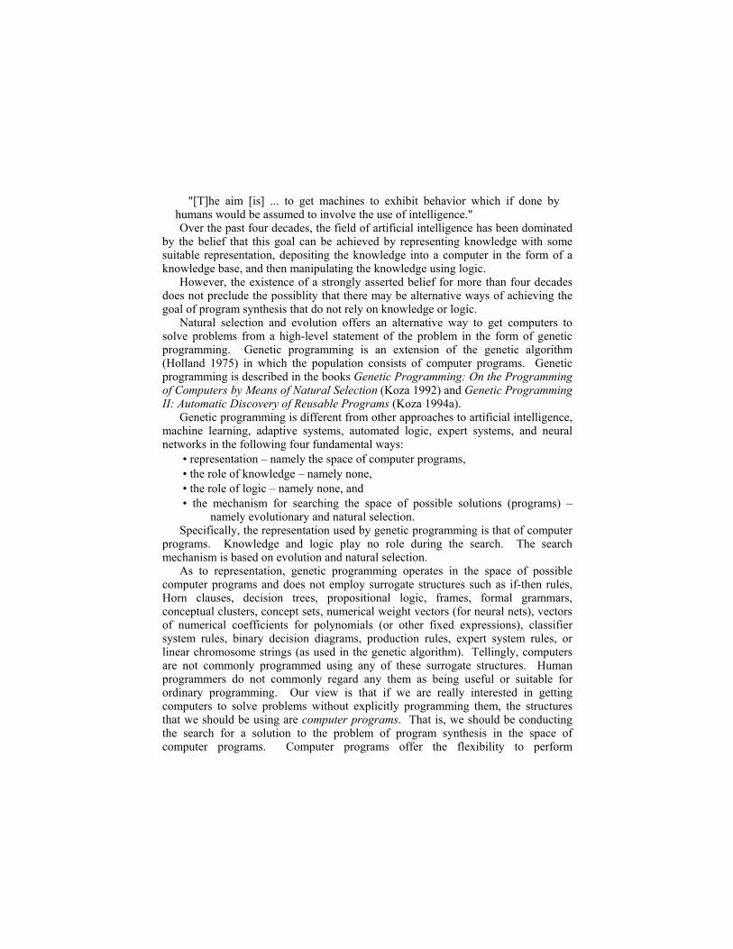
Figure 1 shows a one-input, one-output embryonic circuit in which VSOURCE is the input signal and VOUT is the output signal (the probe point). The circuit is driven by an incoming alternating circuit source VSOURCE. There is a fixed load resistor RLOAD and a fixed source resistor RSOURCE in the embryo. In addition

to the fixed components, there is a modifiable wire Z0 between nodes 2 and 3. All development originates from this modifiable wire.

Figure 1 One-input, one-output embryo. 3.2. Component-Creating

Functions Each program tree contains component-creating functions and topology-modifying functions. The component-creating functions insert a component into the developing circuit and assign component value(s) to the component.

Each component-creating functions has a writing head that points to an associated highlighted component in the developing circuit and modifies that component in a specified manner. The construction-continuing subtree of each component-creating functions points to a successor function or terminal in the circuit-constructing program tree.

The arithmetic-performing subtree of a component-creating functions consists of a composition of arithmetic functions (addition and subtraction) and random constants (in the range -1.000 to +1.000). The arithmetic-performing subtree specifies the numerical value of a component by returning a floating-point value that is interpreted on a logarithmic scale as the value for the component in a range of 10 orders of magnitude (using a unit of measure that is appropriate for the particular type of component).

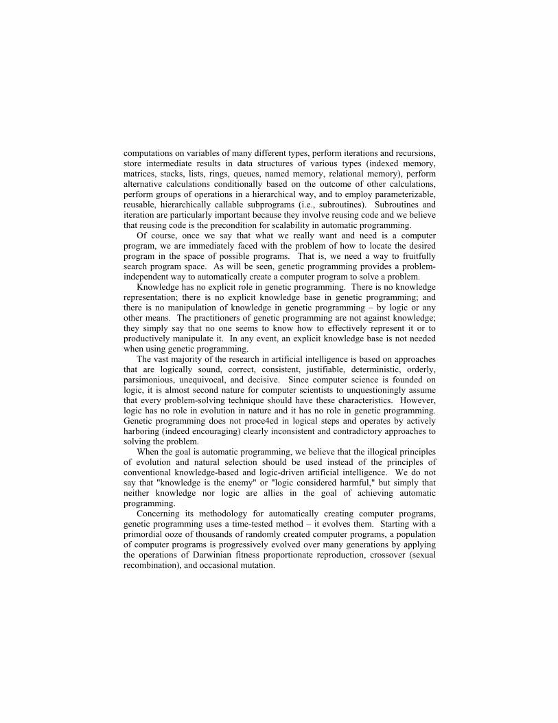
The two-argument resistor-creating R function causes the highlighted component to be changed into a resistor. The value of the resistor in kilo Ohms is specified by its arithmetic-performing subtree.

Figure 2 shows a modifiable wire Z0 connecting nodes 1 and 2 of a partial circuit containing four capacitors (C2, C3, C4, and C5). The circle indicates that Z0 has a writing head (i.e., is the highlighted component and that Z0 is subject to subsequent modification). Figure 3 shows the result of applying the R function to the modifiable wire Z0 of figure 2. The circle indicates that the newly created R1 has a writing head so that R1 remains subject to subsequent modification.

Similarly, the two-argument capacitor-creating C function causes the highlighted component to be changed into a capacitor whose value in micro Farads is specified by its arithmetic-performing subtrees.

The one-argument Q_D_PNP diode-creating function causes a diode to be inserted in lieu of the highlighted component. This function has only one argument because there is no numerical value associated with a diode and thus no arithmetic-performing subtree. In practice, the diode is implemented here using a pnp transistor whose collector and base are connected to each other. The Q_D_NPN function inserts a diode using an npn transistor in a similar manner.

There are also six one-argument transistor-creating functions (Q_POS_COLL_NPN, Q_GND_EMIT_NPN, Q_NEG_EMIT_NPN, Q_GND_EMIT_PNP, Q_POS_EMIT_PNP, Q_NEG_COLL_PNP) that insert a bipolar junction transistor in lieu of the highlighted component and that directly connect the collector or emitter of the newly created transistor to a fixed point of the circuit (the positive power supply, ground, or the negative power supply). For example, the Q_POS_COLL_NPN function inserts a bipolar junction transistor whose collector is connected to the positive power supply.

Figure 2 Modifiable wire Z0. Each of the functions in the family of six different three-argument transistor-

creating Q_3_NPN functions causes an npn bipolar junction transistor to be inserted in place of the highlighted component and one of the nodes to which the highlighted component is connected. The Q_3_NPN function creates five new nodes and three new modifiable wires. There is no writing head on the new transistor, but there is one on the new modifiable wires. There are 12 members (called Q_3_NPN0, ..., Q_3_NPN11) in this family of functions because there are two choices of nodes (1 and 2) to be bifurcated and then there are six ways of attaching the transistor's base, collector, and emitter after the bifurcation. Similarly the family of 12 Q_3_PNP functions causes a pnp bipolar junction transistor to be inserted.

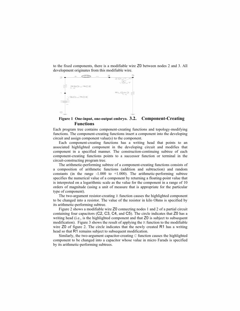
Figure 3 Result of applying the R function.

3.3. Topology-Modifying Functions Each topology-modifying function in a program tree points to an associated highlighted component and modifies the topology of the developing circuit.

The three-argument SERIES division function creates a series composition of the highlighted component (with a writing head), a copy of it (with a writing head), one new modifiable wire (with a writing head), and two new nodes.

The four-argument PARALLEL0 parallel division function creates a parallel composition consisting of the original highlighted component (with a writing head), a copy of it (with a writing head), two new modifiable wires (each with a writing head), and two new nodes. Figure 4 shows the result of applying PARALLEL0 to resistor R1 from figure 3.

Figure 4 Result of the PARALLEL0 function.The one-argument polarity-

reversing FLIP function reverses the polarity of the highlighted component. There are six three-argument functions (T_GND_0, T_GND_1, T_POS_0,

T_POS_1, T_NEG_0, T_NEG_1) that insert two new nodes and two new modifiable wires, and then make a connection to ground, positive power supply, or negative power supply, respectively.

There are two three-argument functions (PAIR_CONNECT_0 and PAIR_CONNECT_1) that enable distant parts of a circuit to be connected together. The first PAIR_CONNECT to occur in the development of a circuit creates two new wires, two new nodes, and one temporary port. The next PAIR_CONNECT creates

two new wires and one new node, connects the temporary port to the end of one of these new wires, and then removes the temporary port.

The one-argument NOOP function has no effect on the highlighted component; however, it delays activity on the developmental path on which it appears in relation to other developmental paths in the overall program tree.

The zero-argument END function causes the highlighted component to lose its writing head, thereby ending that particular developmental path.

The zero-argument SAFE_CUT function causes the highlighted component to be removed from the circuit provided that the degree of the nodes at both ends of the highlighted component is three (i.e., no dangling components or wires are created).

4. Preparatory Steps Before applying genetic programming to a problem of circuit design, seven major preparatory steps are required: (1) identify the suitable embryonic circuit, (2) determine the architecture of the overall circuit-constructing program trees, (3) identify the terminals of the program trees, (4) identify the primitive functions contained in these program trees, (5) create the fitness measure, (6) choose parameters, and (7) determine the termination criterion and method of result designation.

4.1. Embryonic Circuit The embryonic circuit used on a particular problem depends on the circuit's number of inputs and outputs.

For example, in the robot controller circuit, the circuit has two inputs, VSOURCE1 and VSOURCE2, not just one. Moreover, each input needs its own separate source resistor (RSOURCE1 and RSOURCE2). Consequently, the embryo has three modifiable wires Z0, Z1, and Z2 in order to provide full connectivity between the two inputs and the one output. All development then originates from these three modifiable wires.

There is often considerable flexibility in choosing the embryonic circuit. For example, an embryo with two modifiable wires (Z0 and Z1) was used for the lowpass filter. In some problems, such as the amplifier, the embryo contains additional fixed components because of additional problem-specific functionality of the harness (as described in Koza, Bennett, Andre, and Keane 1997).

4.2. Program Architecture Since there is one result-producing branch in the program tree for each modifiable wire in the embryo, the architecture of each circuit-constructing program tree depends on the embryonic circuit. One result-producing branch was used for the frequency discriminator and the computational circuit; two were used for lowpass filter problem; and three were used for the robot controller and amplifier. The

architecture of each circuit-constructing program tree also depends on the use, if any, of automatically defined functions. Automatically defined functions and architecture-altering operations were used in the frequency discriminator, robot controller, and amplifier. For these problems, each program in the initial population of programs had a uniform architecture with no automatically defined functions. In later generations, the number of automatically defined functions, if any, emerged as a consequence of the architecture-altering operations.

4.3. Function and Terminal Sets The function set for each design problem depended on the type of electrical components that were used to construct the circuit. Inductors and capacitors were used for the lowpass and highpass filter problems. Capacitors, diodes, and transistors were used for the computational circuit, the robot controller, and the amplifier. Resistors (in addition to inductors and capacitors) were used for the frequency discriminator. When transistors were used, functions to provide connectivity to the positive and negative power supplies were also included.

For the computational circuit, the robot controller, and the amplifier, the function set, Fccs-initial, for each construction-continuing subtree was

Fccs-initial = {R, C, SERIES, PARALLEL0, PARALLEL1, FLIP, NOOP, T_GND_0, T_GND_1, T_POS_0, T_POS_1, T_NEG_0, T_NEG_1, PAIR_CONNECT_0, PAIR_CONNECT_1, Q_D_NPN, Q_D_PNP, Q_3_NPN0, ..., Q_3_NPN11, Q_3_PNP0, ..., Q_3_PNP11, Q_POS_COLL_NPN, Q_GND_EMIT_NPN, Q_NEG_EMIT_NPN, Q_GND_EMIT_PNP, Q_POS_EMIT_PNP, Q_NEG_COLL_PNP}.

For the npn transistors, the Q2N3904 model was used. For pnp transistors, the Q2N3906 model was used.

The initial terminal set, Tccs-initial, for each construction-continuing subtree was

Tccs-initial = {END, SAFE_CUT}.

The initial terminal set, Taps-initial, for each arithmetic-performing subtree consisted of

Taps-initial = {←},

where ← represents floating-point random constants from –1.0 to +1.0. The function set, Faps, for each arithmetic-performing subtree was,

Faps = {+, -}.

The terminal and function sets were identical for all result-producing branches for a particular problem.

For the lowpass filter and frequency discriminator, there was no need for functions to provide connectivity to the positive and negative power supplies.

For the frequency discriminator, the robot controller, and the amplifier, the architecture-altering operations were used and the set of potential new functions, Fpotential, was

Fpotential = {ADF0, ADF1, ...}.

The set of potential new terminals, Tpotential, for the automatically defined functions was

Tpotential = {ARG0}.

The architecture-altering operations change the function set, Fccs for each construction-continuing subtree of all three result-producing branches and the function-defining branches, so that

Fccs = Fccs-initial ≈ Fpotential.

The architecture-altering operations generally change the terminal set for automatically defined functions, Taps-adf, for each arithmetic-performing subtree, so that

Taps-adf = Taps-initial ≈ Tpotential.

4.4. Fitness Measure The fitness measure varies for each problem. The high-level statement of desired circuit behavior is translated into a well-defined measurable quantity that can be used by genetic programming to guide the evolutionary process. The evaluation of each individual circuit-constructing program tree in the population begins with its execution. This execution progressively applies the functions in each program tree to an embryonic circuit, thereby creating a fully developed circuit. A netlist is created that identifies each component of the developed circuit, the nodes to which each component is connected, and the value of each component. The netlist becomes the input to the 217,000-line SPICE (Simulation Program with Integrated Circuit Emphasis) simulation program (Quarles, Newton, Pederson, and Sangiovanni-Vincentelli 1994). SPICE then determines the behavior of the circuit. It was necessary to make considerable modifications in SPICE so that it could run as a submodule within the genetic programming system.

4.4.1 Lowpass Filter A simple filter is a one-input, one-output electronic circuit that receives a signal as its input and passes the frequency components of the incoming signal that lie in a

specified range (called the passband) while suppressing the frequency components that lie in all other frequency ranges (the stopband).

The desired lowpass LC filter should have a passband below 1,000 Hz and a stopband above 2,000 Hz. The circuit is driven by an incoming AC voltage source with a 2 volt amplitude. If the source (internal) resistance RSOURCE and the load resistance RLOAD in the embryonic circuit are each 1 kilo Ohm, the incoming 2 volt signal is divided in half.

The attenuation of the filter is defined in terms of the output signal relative to the reference voltage (half of 2 volt here). A decibel is a unitless measure of relative voltage that is defined as 20 times the common (base 10) logarithm of the ratio between the voltage at a particular probe point and a reference voltage.

In this problem, a voltage in the passband of exactly 1 volt and a voltage in the stopband of exactly 0 volts is regarded as ideal. The (preferably small) variation within the passband is called the passband ripple. Similarly, the incoming signal is never fully reduced to zero in the stopband of an actual filer. The (preferably small) variation within the stopband is called the stopband ripple. A voltage in the passband of between 970 millivolts and 1 volt (i.e., a passband ripple of 30 millivolts or less) and a voltage in the stopband of between 0 volts and 1 millivolts (i.e., a stopband ripple of 1 millivolts or less) is regarded as acceptable. Any voltage lower than 970 millivolts in the passband and any voltage above 1 millivolts in the stopband is regarded as unacceptable.

A fifth-order elliptic (Cauer) filter with a modular angle Θ of 30 degrees (i.e., the arcsin of the ratio of the boundaries of the passband and stopband) and a reflection coefficient ρ of 24.3% is required to satisfy these design goals.

Since the high-level statement of behavior for the desired circuit is expressed in terms of frequencies, the voltage VOUT is measured in the frequency domain. SPICE performs an AC small signal analysis and report the circuit's behavior over five decades (between 1 Hz and 100,000 Hz) with each decade being divided into 20 parts (using a logarithmic scale), so that there are a total of 101 fitness cases.

Fitness is measured in terms of the sum over these cases of the absolute weighted deviation between the actual value of the voltage that is produced by the circuit at the probe point VOUT and the target value for voltage. The smaller the value of fitness, the better. A fitness of zero represents an (unattainable) ideal filter.

Specifically, the standardized fitness is

F(t) = i=0

100∑ (W (d ( f i ), f i )d ( f i ))

where fi is the frequency of fitness case i; d(x) is the absolute value of the difference between the target and observed values at frequency x; and W(y,x) is the weighting for difference y at frequency x.

The fitness measure is designed to not penalize ideal values, to slightly penalize every acceptable deviation, and to heavily penalize every unacceptable deviation. Specifically, the procedure for each of the 61 points in the 3-decade interval between 1 Hz and 1,000 Hz for the intended passband is as follows:

• If the voltage equals the ideal value of 1.0 volt in this interval, the deviation is 0.0.

• If the voltage is between 970 millivolts and 1 volt, the absolute value of the deviation from 1 volt is weighted by a factor of 1.0.

• If the voltage is less than 970 millivolts, the absolute value of the deviation from 1 volt is weighted by a factor of 10.0.

The acceptable and unacceptable deviations for each of the 35 points from 2,000 Hz to 100,000 Hz in the intended stopband are similarly weighed (by 1.0 or 10.0) based on the amount of deviation from the ideal voltage of 0 volts and the acceptable deviation of 1 millivolts.

For each of the five "don't care" points between 1,000 and 2,000 Hz, the deviation is deemed to be zero.

The number of “hits” for this problem (and all other problems herein) is defined as the number of fitness cases for which the voltage is acceptable or ideal or that lie in the "don't care" band (for a filter).

Many of the random initial circuits and many that are created by the crossover and mutation operations in subsequent generations cannot be simulated by SPICE. These circuits receive a high penalty value of fitness (108) and become the worst-of-generation programs for each generation.

For details, see Koza, Bennett, Andre, and Keane 1996b.

4.4.2 Tri-state Frequency Discriminator Fitness is the sum, over 101 fitness cases, of the absolute weighted deviation between the actual value of the voltage that is produced by the circuit and the target value.

The three points that are closest to the band located within 10% of 256 Hz are 229.1 Hz, 251.2 Hz, and 275.4 Hz. The procedure for each of these three points is as follows: If the voltage equals the ideal value of 1/2 volts in this interval, the deviation is 0.0. If the voltage is more than 240 millivolts from 1/2 volts, the absolute value of the deviation from 1/2 volts is weighted by a factor of 20. If the voltage is more than 240 millivolts of 1/2 volts, the absolute value of the deviation from 1/2 volts is weighted by a factor of 200. This arrangement reflects the fact that the ideal output voltage for this range of frequencies is 1/2 volts, the fact that a 240 millivolts discrepancy is acceptable, and the fact that a larger discrepancy is not acceptable.

Similar weighting was used for the three points (2,291 Hz, 2,512 Hz, and 2,754 Hz) that are closest to the band located within 10% of 2,560 ,Hz.

The procedure for each of the remaining 95 points is as follows: If the voltage equals the ideal value of 0 volts, the deviation is 0.0. If the voltage is within 240 millivolts of 0 volts, the absolute value of the deviation from 0 volts is weighted by a factor of 1.0. If the voltage is more than 240 millivolts from 0 volts, the absolute value of the deviation from 0 volts is weighted by a factor of 10. For details, see Koza, Bennett, Lohn, Dunlap, Andre, and Keane 1997b.

4.4.3 Computational Circuit SPICE is called to perform a DC sweep analysis at 21 equidistant voltages between –250 millivolts and +250 millivolts. Fitness is the sum, over these 21 fitness cases, of the absolute weighted deviation between the actual value of the voltage that is produced by the circuit and the target value for voltage. For details, see Koza, Bennett, Lohn, Dunlap, Andre, and Keane 1997a.

4.4.4 Robot Controller Circuit The fitness of a robot controller was evaluated using 72 randomly chosen fitness cases each representing a different target point. Fitness is the sum, over the 72 fitness cases, of the travel times. If the robot came within a capture radius of 0.28 meters of its target point before the end of the 80 time steps allowed for a particular fitness case, the contribution to fitness for that fitness case was the actual time. However, if the robot failed to come within the capture radius during the 80 time steps, the contribution to fitness was 0.160 hours (i.e., double the worst possible time).

SPICE performs a nested DC sweep, which provides a way to simulate the DC behavior of a circuit with two inputs. It resembles a nested pair of FOR loops in a computer program in that both of the loops have a starting value for the voltage, an increment, and an ending value for the voltage. For each voltage value in the outer loop, the inner loop simulates the behavior of the circuit by stepping through its range of voltages. Specifically, the starting value for voltage is –4 volt, the step size is 0.2 volt, and the ending value is +4 volt. These values correspond to the dimensions of the robot's world of 64 square meters extending 4 meters in each of the four directions from the origin of a coordinate system (i.e., 1 volt equals 1 meter). For details, see Koza, Bennett, Keane, and Andre 1997.

4.4.5 60 dB Amplifier SPICE was requested to perform a DC sweep analysis to determine the circuit's response for several different DC input voltages. An ideal inverting amplifier circuit would receive the DC input, invert it, and multiply it by the amplification factor. A circuit is flawed to the extent that it does not achieve the desired amplification, the output signal is not perfectly centered on 0 volts(i.e., it is biased), or the DC response is not linear. Fitness is calculated by summing an amplification penalty, a

bias penalty, and two non-linearity penalties – each derived from these five DC outputs. For details, see Bennett, Koza, Andre, and Keane 1996.

4.5. Control Parameters The population size, M, was 640,000 for all problems. Other parameters were substantially the same for each of the five problems and can be found in the references cited above.

4.6. Implementation on Parallel Computer Each problem was run on a medium-grained parallel Parsytec computer system (Andre and Koza 1996) consisting of 64 80-MHz PowerPC 601 processors arranged in an 8 by 8 toroidal mesh with a host PC Pentium type computer. The distributed genetic algorithm was used with a population size of Q = 10,000 at each of the D = 64 demes (semi-isolated subpopulations). On each generation, four boatloads of emigrants, each consisting of B = 2% (the migration rate) of the node's subpopulation (selected on the basis of fitness) were dispatched to each of the four adjacent processing nodes.

5. Results In all five problems, fitness was observed to improve over successive generations. A large majority of the randomly created initial circuits of generation 0 were not able to be simulated by SPICE; however, most were simulatable after only a few generations. Satisfactory results were generated in every case on the first or second trial. When two runs were required, the first produced an almost satisfactory result. This rate of success suggests that the capabilities of the approach and current computing system have not been fully exploited.

5.1. Lowpass Filter Many of the runs produced lowpass filters having a topology similar to that employed by human engineers. For example, in generation 32 of one run, a circuit (figure 5) was evolved with a near-zero fitness of 0.00781. The circuit was 100% compliant with the design requirements in that it scored 101 hits (out of 101). After the evolutionary run, this circuit (and all evolved circuits herein) were simulated anew using the commercially available MicroSim circuit simulator to verify performance. This circuit had the recognizable ladder topology (46) of a Butterworth or Chebychev filter (i.e., a composition of series inductors horizontally with capacitors as vertical shunts).

Figure 6 shows the behavior in the frequency domain of this evolved lowpass filter. As can be seen, the evolved circuit delivers about 1 volt for all frequencies up to 1,000 Hz and about 0 volts for all frequencies above 2,000 Hz.

In another run, a 100% compliant recognizable "bridged T" arrangement was evolved. In yet another run using automatically defined functions, a 100% compliant circuit emerged with the recognizable elliptic topology that was invented and patented by Cauer. When invented. the Cauer filter was a significant advance (both theoretically and commercially) over the Butterworth and Chebychev filters.

Thus, genetic programming rediscovered the ladder topology of the Butterworth and Chebychev filters, the "bridged T" topology, and the elliptic topology.

Figure 5 Evolved 7-rung ladder lowpass filter.

Figure 6 Frequency domain behavior of genetically evolved 7-rung ladder

lowpass filter.

Figure 7 Evolved frequency discriminator.

5.2. Tri-state Frequency Discriminator The evolved three-way tri-state frequency discriminator circuit from generation 106 scores 101 hits (out of 101). Figure 7 shows this circuit (after expansion of its automatically defined functions). The circuit produces the desired outputs of 1 volt and 1/2 volts (each within the allowable tolerance) for the two specified bands of frequencies and the desired near-zero signal for all other frequencies.

5.3. Computational Circuit The genetically evolved computational circuit for the square root from generation 60 (figure 8), achieves a fitness of 1.68, and has 36 transistors, two diodes, no capacitors, and 12 resistors (in addition to the source and load resistors in the embryo). The output voltages produced by this best-of-run circuit are almost exactly the required values.

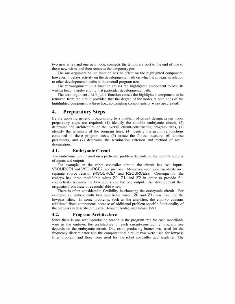
5.4. Robot Controller Circuit The best-of-run time-optimal robot controller circuit (figure 9) appeared in generation 31, scores 72 hits, and achieves a near-optimal fitness of 1.541 hours. In comparison, the optimal value of fitness for this problem is known to be 1.518 hours. This best-of-run circuit has 10 transistors and 4 resistors. The program has one automatically defined function that is called twice (incorporated into the figure).

5.5. 60 dB Amplifier The best circuit from generation 109 (figure 10) achieves a fitness of 0.178. Based on a DC sweep, the amplification is 60 dB here (i.e., 1,000-to-1 ratio) and the bias is

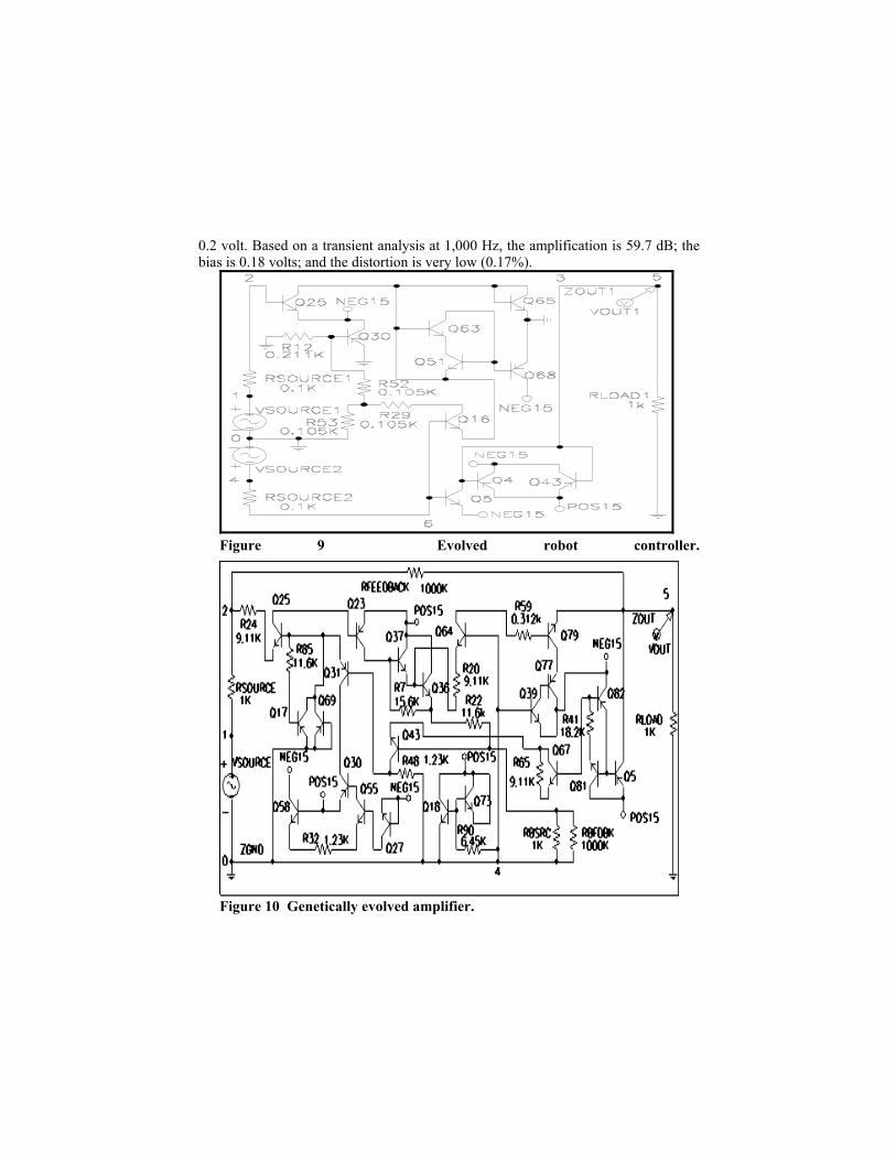
0.2 volt. Based on a transient analysis at 1,000 Hz, the amplification is 59.7 dB; the bias is 0.18 volts; and the distortion is very low (0.17%).

Figure 9 Evolved robot controller.

Figure 10 Genetically evolved amplifier.

Based on an AC sweep, the amplification at 1,000 Hz is 59.7 dB; the flatband gain is 60 dB; and the 3 dB bandwidth is 79, 333 Hz. Thus, a high-gain amplifier with low distortion and acceptable bias has been evolved.

6. Other Circuits Numerous other circuits have been similarly designed, including asymmetric bandpass filters (Koza, Bennett, Andre, and Keane 1996c), crossover filters (Koza, Bennett, Andre, and Keane 1996a), comb filters (Koza, Andre, Bennett, and Keane 1996), amplifiers (Koza, Bennett, Andre, and Keane 1997), a temperature sensor, and a voltage reference circuit (Koza, Bennett, Andre, Keane, and Dunlap 1997).

Figure 8 Evolved square root circuit.

7. Conclusion Genetic programming evolved the topology and sizing of five different prototypical analog electrical circuits.

References Aaserud, O. and Nielsen, I. Ring. 1995. Trends in current analog design: A panel

debate. Analog Integrated Circuits and Signal Processing. 7(1) 5-9. Andre, David and Koza, John R. 1996. Parallel genetic programming: A scalable

implementation using the transputer architecture. In Angeline, P. J. and Kinnear, K. E. Jr. (editors). 1996. Advances in Genetic Programming 2. Cambridge: MIT Press.

Angeline, Peter J. and Kinnear, Kenneth E. Jr. (editors). 1996. Advances in Genetic Programming 2. Cambridge, MA: The MIT Press.

Banzhaf, Wolfgang, Nordin, Peter, Keller, Robert E., and Francone, Frank D. 1998. Genetic Programming – An Introduction. San Francisco, CA: Morgan Kaufmann and Heidelberg: dpunkt.

Bennett III, Forrest H, Koza, John R., Andre, David, and Keane, Martin A. 1996. Evolution of a 60 Decibel op amp using genetic programming. In Higuchi, Tetsuya, Iwata, Masaya, and Lui, Weixin (editors). Proceedings of International Conference on Evolvable Systems: From Biology to Hardware (ICES-96). Lecture Notes in Computer Science, Volume 1259. Berlin: Springer-Verlag. Pages 455-469.

Brave, Scott. 1996. Evolving deterministic finite automata using cellular encoding. In Koza, John R., Goldberg, David E., Fogel, David B., and Riolo, Rick L. (editors). 1996. Genetic Programming 1996: Proceedings of the First Annual Conference, July 28-31, 1996, Stanford University. Cambridge, MA: MIT Press. Pages 39–44.

Grimbleby, J. B. 1995. Automatic analogue network synthesis using genetic algorithms. Proceedings of the First International Conference on Genetic Algorithms in Engineering Systems: Innovations and Applications. London: Institution of Electrical Engineers. Pages 53–58.

Gruau, Frederic. 1992. Cellular Encoding of Genetic Neural Networks. Technical report 92-21. Laboratoire de l'Informatique du Parallélisme. Ecole Normale Supérieure de Lyon. May 1992.

Holland, John H. 1975. Adaptation in Natural and Artificial Systems. Ann Arbor, MI: University of Michigan Press.

Kinnear, Kenneth E. Jr. (editor). 1994. Advances in Genetic Programming. Cambridge, MA: The MIT Press.

Kitano, Hiroaki. 1990. Designing neural networks using genetic algorithms with graph generation system. Complex Systems. 4(1990) 461–476.

Koza, John R. 1992. Genetic Programming: On the Programming of Computers by Means of Natural Selection. Cambridge, MA: MIT Press.

Koza, John R. 1994a. Genetic Programming II: Automatic Discovery of Reusable Programs. Cambridge, MA: MIT Press.

Koza, John R. 1994b. Genetic Programming II Videotape: The Next Generation. Cambridge, MA: MIT Press.

Koza, John R. 1995. Evolving the architecture of a multi-part program in genetic programming using architecture-altering operations. In McDonnell, John R., Reynolds, Robert G., and Fogel, David B. (editors). 1995. Evolutionary Programming IV: Proceedings of the Fourth Annual Conference on Evolutionary Programming. Cambridge, MA: The MIT Press. Pages 695–717.

Koza, John R., Andre, David, Bennett III, Forrest H, and Keane, Martin A. 1996. Use of automatically defined functions and architecture-altering operations in automated circuit synthesis using genetic programming. In Koza, John R., Goldberg, David E., Fogel, David B., and Riolo, Rick L. (editors). 1996. Genetic Programming 1996: Proceedings of the First Annual Conference. Cambridge, MA: The MIT Press.

Koza, John R., Bennett III, Forrest H, Andre, David, and Keane, Martin A. 1996a. Four problems for which a computer program evolved by genetic programming is competitive with human performance. Proceedings of the 1996 IEEE International Conference on Evolutionary Computation. IEEE Press. Pages 1–10.

Koza, John R., Bennett III, Forrest H, Andre, David, and Keane, Martin A. 1996b. Automated design of both the topology and sizing of analog electrical circuits using genetic programming. In Gero, John S. and Sudweeks, Fay (editors). Artificial Intelligence in Design '96. Dordrecht: Kluwer. Pages 151-170.

Koza, John R., Bennett III, Forrest H, Andre, David, and Keane, Martin A. 1996c. Automated WYWIWYG design of both the topology and component values of analog electrical circuits using genetic programming. In Koza, John R., Goldberg, David E., Fogel, David B., and Riolo, Rick L. (editors). 1996. Genetic Programming 1996: Proceedings of the First Annual Conference. Cambridge, MA: The MIT Press.

Koza, John R., Bennett III, Forrest H, Andre, David, and Keane, Martin A. 1997. Evolution using genetic programming of a low-distortion 96 Decibel operational amplifier. Proceedings of the 1997 ACM Symposium on Applied Computing, San Jose, California, February 28 – March 2, 1997. New York: Association for Computing Machinery. Pages 207 - 216.

Koza, John R., Bennett III, Forrest H, Andre, David, Keane, Martin A, and Dunlap, Frank. 1997. Automated synthesis of analog electrical circuits by means of genetic programming. IEEE Transactions on Evolutionary Computation. 1(2). Pages 109 – 128.

Koza, John R., Bennett III, Forrest H, Keane, Martin A., and Andre, David. 1997. Automatic programming of a time-optimal robot controller and an analog electrical circuit to implement the robot controller by means of genetic programming. Proceedings of 1997 IEEE International Symposium on Computational Intelligence in Robotics and Automation. Los Alamitos, CA; Computer Society Press. Pages 340 – 346.

Koza, John R., Bennett III, Forrest H, Lohn, Jason, Dunlap, Frank, Andre, David, and Keane, Martin A. 1997. Automated synthesis of computational circuits using genetic programming. Proceedings of the 1997 IEEE Conference on Evolutionary Computation. Piscataway, NJ: IEEE Press. 447–452.

Koza, John R., Bennett III, Forrest H, Lohn, Jason, Dunlap, Frank, Andre, David, and Keane, Martin A. 1997b. Use of architecture-altering operations to dynamically adapt a three-way analog source identification circuit to accommodate a new source. In Koza, John R., Deb, Kalyanmoy, Dorigo, Marco, Fogel, David B., Garzon, Max, Iba, Hitoshi, and Riolo, Rick L. (editors). 1997. Genetic Programming 1997: Proceedings of the Second Annual Conference. San Francisco, CA: Morgan Kaufmann. 213 – 221.

Koza, John R., Deb, Kalyanmoy, Dorigo, Marco, Fogel, David B., Garzon, Max, Iba, Hitoshi, and Riolo, Rick L. (editors). 1997. Genetic Programming 1997: Proceedings of the Second Annual Conference. San Francisco, CA: Morgan Kaufmann.

Koza, John R., Goldberg, David E., Fogel, David B., and Riolo, Rick L. (editors). 1996. Genetic Programming 1996: Proceedings of the First Annual Conference. Cambridge, MA: The MIT Press.

Koza, John R., and Rice, James P. 1992. Genetic Programming: The Movie. Cambridge, MA: MIT Press.

Kruiskamp Marinum Wilhelmus and Leenaerts, Domine. 1995. DARWIN: CMOS opamp synthesis by means of a genetic algorithm. Proceedings of the 32nd Design Automation Conference. New York, NY: Association for Computing Machinery. Pages 433–438.

Quarles, Thomas, Newton, A. R., Pederson, D. O., and Sangiovanni-Vincentelli, A. 1994. SPICE 3 Version 3F5 User's Manual. Department of Electrical Engineering and Computer Science, University of California, Berkeley, CA. March 1994.

Rutenbar, R. A. 1993. Analog design automation: Where are we? Where are we going? Proceedings of the l5th IEEE CICC. New York: IEEE. 13.1.1-13.1.8.

Samuel, Arthur L. 1959. Some studies in machine learning using the game of checkers. IBM Journal of Research and Development. 3(3): 210–229.

Samuel, Arthur L. 1983. AI: Where it has been and where it is going. Proceedings of the Eighth International Joint Conference on Artificial Intelligence. Los Altos, CA: Morgan Kaufmann. Pages 1152 – 1157.

Thompson, Adrian. 1996. Silicon evolution. In Koza, John R., Goldberg, David E., Fogel, David B., and Riolo, Rick L. (editors). 1996. Genetic Programming 1996: Proceedings of the First Annual Conference. Cambridge, MA: MIT Press.

Version 2 – Submitted December 21, 1997 for Computational Intelligence and Software Engineering to be edited by Witold Pedrycz and Jim F. Peters of the University of Manitolba for World Scientific.

AUTOMATIC CREATION OF COMPUTER PROGRAMS FOR DESIGNING ELECTRICAL CIRCUITS USING GENETIC

PROGRAMMING

J. R. Koza Computer Science Dept., Stanford University, Stanford, CA 94305

E-mail: koza@cs.stanford.edu http://www-cs-faculty.stanford.edu/~koza/

F. H Bennett III

Visiting Scholar, Computer Science Dept., Stanford University, Stanford, CA 94305

E-mail: forrest@evolute.com

D. Andre Computer Science Division University of California, Berkeley, CA

E-mail: dandre@cs.berkeley.edu

M. A. Keane Martin Keane Inc., 5733 West Grover, Chicago, Illinois 60630

E-mail: makeane@ix.netcom.com KEYWORDS: Genetic programming, genetic algorithms, design, circuit synthesis, analog

electrical circuits, electrical circuits, artificial intelligence, machine learning, program synthesis, automatic programming, filter, amplifier, controller.

TO: Prof. Witold Pedrycz Dept. of Electrical and Computer Engineering University of Manitoba Winnipeg, Manitoba R3T 5V6 Canada