author's personal copy -...

This article was published in an Elsevier journal. The attached copyis furnished to the author for non-commercial research and

education use, including for instruction at the author’s institution,sharing with colleagues and providing to institution administration.

Other uses, including reproduction and distribution, or selling orlicensing copies, or posting to personal, institutional or third party

websites are prohibited.

In most cases authors are permitted to post their version of thearticle (e.g. in Word or Tex form) to their personal website orinstitutional repository. Authors requiring further information

regarding Elsevier’s archiving and manuscript policies areencouraged to visit:

http://www.elsevier.com/copyright

http://www.elsevier.com/copyright

Author's personal copy

Biochemical Engineering Journal 39 (2008) 190–206

Bioprocess hybrid parametric/nonparametric modellingbased on the concept of mixture of experts

J. Peres a, R. Oliveira b, S. Feyo de Azevedo a,∗a Department of Chemical Engineering, Faculty of Engineering, University of Porto, Rua Dr. Roberto Frias s/n, 4200-465 Porto, Portugal

b REQUIMTE/CQFB, Departamento de Quımica, Faculdade de Ciencias e Tecnologia, Universidade Nova de Lisboa,P-2829-516 Caparica, Portugal

Received 21 March 2006; received in revised form 7 September 2007; accepted 17 September 2007

Abstract

This paper presents a novel method for bioprocess hybrid parametric/nonparametric modelling based on mixture of experts (ME) and theexpectation maximisation (EM) algorithm. The bioreactor system is described by material balance equations whereas the cell population subsystemis described by an adjustable mixture of parametric/nonparametric sub-models inspired in the ME architecture. This idea was motivated by thefact that cellular metabolism has an inherent “modular” structure, organised in metabolic pathways, with complex interactions. This study wassupported by simulations using models of different levels of complexity. The proposed method was compared with the conventional hybridtechnique employing the multi-layer perceptron (MLP) and the radial basis function (RBF) networks. As main conclusions it can be stated thatMEs trained with the EM algorithm are able to systematically detect metabolic shifts with the individual experts developing expertise in describingthe individual pathways. The hybrid ME model with thin-plate spline RBF network as experts outperforms both the hybrid MLP model and thehybrid RBF model in its ability to describe metabolic switches.© 2007 Elsevier B.V. All rights reserved.

Keywords: Bioprocesses; Bioreactors; Hybrid modelling; Mixture of experts; Expectation maximisation; Artificial intelligence; Waste-water treatment; Control

1. Introduction

The development of optimal control strategies for bio-processes is frequently constrained by the availability ofsufficiently accurate mathematical models for supporting suchdevelopments. Bioprocesses may be generically characterisedas complex systems exhibiting non-linear and time-varyingdynamics. The main source of complexity arises from theintracellular phenomena. Model-based bioreactor performanceoptimisation studies rarely incorporate detailed descriptions ofthe intracellular phase. The method is often viewed as being too“expensive” for routine applications. It has been pointed out byseveral authors that hybrid parametric/nonparametric modellingtechniques may represent a cost-effective alternative for the anal-ysis of bioprocesses [1–6]. Hybrid parametric/nonparametricsystems combine first principles modelling with chemometrictechniques for extracting knowledge hidden in process data;

∗ Corresponding author. Tel.: +351 225081694; fax: +351 225081632.E-mail address: [email protected] (S.F. de Azevedo).

hidden knowledge that has not been incorporated in the firstprinciples submodels so far. The most widely adopted hybridstructure for bioreactor systems combines macroscopic materialand/or energy balance equations with artificial neural networkssuch as the MLP or the RBF networks [4,7–17]. The job forthe neural networks in these structures is the nonparametricmodelling of unknown reaction kinetics, which is normallythe most challenging part of the process to be modelled ina mechanistic sense. One important feature of living cells isthe fact that they process different substrates through differ-ent metabolic pathways. Diauxic growth on two carbon sourcesis one of such examples. Another is aerobic/anaerobic growth,depending on the presence or absence of dissolved oxygen inthe medium. For example, the Saccharomyces cerevisiae yeastgrows through three different metabolic pathways for exploitingenergy and basic material sources and is able to switch betweena oxidative metabolic state and a oxido-reductive metabolicstate [18]. With high glucose supply or in conditions of oxygenlimitation, Escherichia coli produces acetate via an alterna-tive pathway. In case of glucose limitation, E. coli is able toalternatively metabolise acetate [e.g. 19]. In the more com-

1369-703X/$ – see front matter © 2007 Elsevier B.V. All rights reserved.doi:10.1016/j.bej.2007.09.003


J. Peres et al. / Biochemical Engineering Journal 39 (2008) 190–206 191

plex example of mixed cultures, several different metabolicmechanisms may occur simultaneously. In activated sludge pro-cesses, three main families of bacteria are involved, each ofthem switching between metabolic mechanisms [20] yieldingcomplex kinetic behaviour, viz. nitrification/denitrification, aer-obic/anaerobic, phosphorus accumulation/release states. Thebiological systems exemplified have inherent non-linear discon-tinuous reaction kinetics due to switching between metabolicmechanisms. The popular MLP networks have some limitationsfor approximating discontinuous input–output systems. MLPstend to exhibit erratic behaviour around discontinuities [21].RBF networks have the capacity of capturing the underlyinglocal struture of the input–output mapping [21] and could bemore suitable for processes with discontinuities. [22] showedthat modular neural networks, such as the ME [23], are wellsuited for the identification of processes that switch betweendifferent operating conditions. Such modular network architec-tures might be an interesting alternative for bioprocess hybridmodelling. A modular network architecture consists of two ormore (small) network modules mediated by an integration unit,which decides how to combine their outputs to form the finalsystem output and which modules should learn which trainingpatterns [21]. This type of architecture performs task decompo-sition in the sense that it learns to partition a task into two or morefunctionally independent tasks and allocates distinct networks tolearn each task [23]. As already mentioned, cells reaction kinet-ics are ruled by a rather complex network of metabolic reactionsorganised in different pathways: glycolysis, tricarboxylic acidcycle and many other. Hence a modular network structure ishypothetically highly compatible with the internal structure ofthe cell system. The main objective of this work is to developa hybrid modelling method for bioprocesses accounting for theintracellular modular structure of the cells subsystem. The com-bination of first principles modelling with modular networkarchitectures is thus explored. The remaining of this paper isorganised in four more sections. In Section 2 a general hybridstructure for bioreactor systems is described. Following, the MEnetwork architecture and the expectation maximisation (EM)algorithm are reviewed. The incorporation of these concepts inthe hybrid modelling framework is discussed. In Sections 3.1 and3.2 two case studies are presented where hybrid models employ-

ing mixture of experts, MLPs and RBF networks are compared.Finally, in Section 4, the main conclusions are presented.

2. Proposed hybrid modelling technique

2.1. General parametric/nonparametric hybrid model forbioreactor systems

Hybrid model structures have been classified as paralleland/or serial [7,8]. In parallel structures a full mathematicalmodel is available that however is not sufficiently accuratefor model-based applications. A nonparametric modelling tech-nique is then combined in parallel with the mathematical model,having access to the same input variables and correcting themathematical model outputs. In the serial case, there is knowl-edge concerning the general structure of the system, but partsthereof are not known in a mechanistic sense. Such unknownsub-systems are modelled with nonparametric techniques, whichfeed with information to mechanistic parts. The hybrid modelstructures that naturally arise in bioreactor modelling problemstend to be simultaneously serial and parallel [24,25]. The biore-actor system is described by material balance equations while aparallel neural network/mechanistic structure represents the cellpopulation system. In this work, a similar structure is adoptedthat however uses a ME architecture for modelling the unknownreaction kinetics term instead of the usual MLPs or RBFs net-works (see Fig. 1). This model may be mathematically stated bythe following two equations:

dcdt

= r(c, w) − Dc + u (1)

r = Krmec(c)ϕnonp(c, w) (2)

with c a vector of n concentrations, K a n × m yield coefficientsmatrix, rmec a m × r matrix of mechanistically known kineticexpressions, ϕnonp(c, w) a vector of r unknown kinetic func-tions modelled with ME networks, w a vector of parameters thatmust be estimated from data, D the dilution rate, and u is a vec-tor of net volumetric input rates (possibly control inputs). Theunknown reaction kinetics ϕnonp(c, w) are thus modelled withME networks as discussed in the remaining of this section.

Fig. 1. Proposed mechanistic/mixture of experts hybrid structure.


192 J. Peres et al. / Biochemical Engineering Journal 39 (2008) 190–206

2.2. The mixture of experts architecture

Different types of modular networks may be designed,depending on the network modules definition, on the integrationunit definition and on the levels of hierarchy. The most well stud-ied network (initial proposal) is the mixture of experts network(also known as associative Gaussian mixture model) [21,23].The ME architecture consists of a set of K expert networks anda gating network (see Fig. 1). Basically, the task of each expertj is to approximate a function fj : c → ϕj over a region of theinput space. The task of the gating system is to assign an expertnetwork to each input vector c. The final system output ϕME isa combination of the expert network outputs:

ϕME =K∑

j=1

gj(c)ϕj(c) (3)

with gj(c) the gating outputs. The ME architecture has strongstatistical foundations since it was inspired by the concept ofmixture models [26]. The expert modules are simple linear func-tions for non-linear regression problems or linear functions witha single output non-linearity for classification problems. In somenon-linear regression problems it may be necessary to use morecomplex non-linear experts. MLP networks with the tangenthyperbolic function in the hidden layers and linear functionsin the output layer are a possible choice [27] and was one of thechosen structure in this work (the other one was a RBF network):

ϕj(c) = w2,j tanh(w1,jc + b1,j) + b2,j (4)

with w1,j and w2,j the weight matrices in the connectionsbetween nodes of layers 1 and 2 and 2 and 3, respec-tively, whereas b1,j and b2,j are bias associated parametervectors. In the following analysis, the parameters associatedwith each expert j are represented in a vector form wj ={w1,j, b1,j, w2,j, b2,j}. Also, different forms for the gating sys-tem have been reported. The softmax function suggested initiallyby [23], is a normalised exponential function of the inputs c andprovides a “soft” hyperplane division [28]. A localised gatingsystem based on Gaussian functions provides “soft” hyper-ellipsoids input space partitions [28,29]. The localised gatingsystem provides more flexible input space partitions and wasadopted in this work. It can be formulated as follows:

gj(c, a) = αjP(c, mj, �j)K∑

i=1

αiP(c, mi, �i)

(5)

P(c, mj, �j) = (2π)−n/2|�j|−1/2

× exp

{−1

2(c − mj)T�−1

j (c − mj)

}(6)

Eq. (6) is a Gaussian distribution with centre mj and covari-ance matrix �j (usually only the diagonal is considered). Eq.(5) establishes a normalised gating output scaled by the scalarparameters αj . In Eq. (5) the variable a is a vectored represen-tation of all gating system parameters a = {αj, mj, �j}.

The ME architecture concept has been extended to includeseveral hierarchical levels being then termed hierarchical mix-ture of experts (HME). The HME is a tree-like structure wherethe input space is subdivided in regions and regions in subregions and so on. This structure is more complex but mayoften outperform the ME network [30]. For the present studythe ME network structure was adopted instead of the HME,for reasons of simplicity since the ME provided satisfactoryresults.

2.3. The expectation maximisation algorithm

The training algorithm to be adopted is tightly connectedwith the nature of the network structure and to the solution char-acteristics sought. The simplest approach is the classical leastsquares employing the gradient descent (GD) algorithm [21,23],with error back-propagation for the calculation of gradients. Thetraining algorithm has also been treated as a maximum likelihoodparameter estimation problem by [23]. The expectation max-imisation (EM) algorithm [31] was derived and applied for thisstructure by [32]. It was shown in [33] that when the objectivefunction is defined as a mean square error the solutions tend to bemore “cooperative”, whereas the maximum likelihood formula-tion with the EM algorithm tends to produce more “competitive”solutions. The EM algorithm was also shown to provide linearconvergence, faster than that obtained with a gradient ascentalgorithm along with a maximum likelihood formulation [34].Since we are particularly interested in competitive learning theEM algorithm was adopted in this work. This algorithm is a two-step iterative procedure [29,32] that for each iteration p can besummarised as follows:

1. E-stepIn the E-step a matrix of posterior probabilities hp = {hp,t

j }is computed as follows:

hp,tj = gj(ct , ap

j )P(dt|ct , wpj )

K∑i=1

gi(ct ,pai)P(dt|ct ,

pwi)

,

j = 1, . . . , K, t = 1, . . . , np (7)

with the subscript index j denoting expert index, the super-script indexes t and p denoting training pattern and iteration,respectively, with np being the number of measured pat-terns. The term P(dt|ct , wp

j ) is the conditional probabilityof a desired target d of dimension nd , given the input c ofdimension nc and given the expert j. For regression problemsa Gaussian probabilistic model with identity covariance isnormally assumed, hence

P(dt|ct , wpj ) = 1

(2π)−nd/2 exp

(−1

2||d − ϕj||2

)(8)

2. M-stepThe M-step consists of a set of K + 1 independent max-

imisation problems. The first K optimisations evaluate new



expert module parameters wj:

wp+1j = argmax

( np∑t=1

hp,tj ln P(dt|ct , wp

j )

),

j = 1, . . . , K (9)

These optimisations must be solved iteratively usingappropriate numerical methods. A quasi-Newton methodwith conjugated gradients (CG) was employed as describedin [35]. The evaluation of gradients was done with errorback-propagation through the expert networks [36]. The lastoptimisation step K + 1 evaluates new parameters for thegating system. In the case of the localised gating network theoptimisation has an exact one-step analytical solution [29]:

αp+1j = 1

np

∑t

hp,tj (10)

mp+1j = 1∑

t

hp,tj

∑t

hp,tj ct (11)

�p+1j = 1∑

t

hp,tj

∑t

hp,tj (ct − mp+1

j )(ct − mp+1j ) (12)

The algorithms described and adopted in this work are avail-able in the form of a Matlab TM toolbox [37].

3. Results and discussion

3.1. Case study A: fed-batch S. cerevisiae cultivationprocess

In this first case study the proposed hybrid modelling tech-nique is applied to a baker’s yeast production process in afed-batch bioreactor. The S. cerevisiae yeast cells metaboliseglucose via two pathways under aerobic conditions: oxida-tive and/or reductive pathways, with ethanol the end productof the reductive pathway. The yeast cells are also able touse ethanol as an alternative substrate, but the ethanol canbe metabolised oxidatively only. Sonnleitner and Kappeli [18]developed a simple unstructured kinetic model based on the res-piratory bottleneck concept (see Appendices A and B for detaileddescription). The model defines three macroscopic reactions forcarbon source utilisation with well-defined stoichiometry:

a1G + b1N + c1O2μo

G→X + f1CO2 + g1H2O

(P1 – oxidative glucose uptake)

a2G + b2Nμr

G→X + e2E + f2CO2 + g2H2O

(P2 – reductive glucose uptake)

e3E + b3N + c3O2μo

E→X + f3CO2 + g3H2O

(P3 – oxidative ethanol uptake)

with X, G, E, N, O2 and CO2 the biomass, glucose, ethanol,ammonia, oxygen and carbon dioxide, respectively suspendedor dissolved in the liquid phase, ai − gi with i =1, 2 or 3 are stoi-chiometric coefficients, and μo

G, μrG and μo

E specific growth ratesassociated with the three macroscopic reactions. The yeast cellsmay find themselves in one of two metabolic states: oxidative oroxido-reductive. In the oxidative metabolic state, only pathways(P1) and (P3) take place. In conditions of oxygen saturation, itmay be shown that the oxidative metabolic state is only possiblefor glucose concentrations lower than 0.042 g/L. The oxido-reductive state, corresponding to pathways (P1) and (P2), occursfor glucose concentrations higher than 0.042 g/L, presumingagain oxygen saturation. The switch between the two metabolicstates is a crisp “if-then” switch. Consequently, pathways (P2)and (P3) are never simultaneous. The main objective in this studyis to evaluate the proposed hybrid modelling technique and inparticular to verify if a mixture of two experts trained with theEM algorithm is capable of distinguishing between the oxidativeand oxido-reductive states, and if the individual experts developexpertise in describing the one or the other metabolic state. Inthe next two examples the focus was on illustrating and enhanc-ing the theoretical capacities of the mixture of experts networkso measurement noise was excluded thus avoiding the issues ofmodel overfitting.

3.1.1. Example A.1: preliminary simulation studySix batches were simulated using the model described in

Appendices A and B yielding a total number of measured pat-terns of np = 606. Details for the data generation are providedin Table 1. To simplify the analysis, oxygen was assumed to benever limiting. In such circumstances the specific growth rate isa function of glucose and ethanol concentrations only (see modelequations in Appendices A and B). The main objective in thisstudy is to compare the ME, MLP and RBF networks in map-ping the relationship between (μ) and the two concentrations(SG) and (SE).

The ME network was configured with K = 2 MLP expertswith equal size {2, 2, 1}. The total number of parameters was 24(9 parameters per expert and 6 parameters for the gating system– the gating had just one input, the glucose concentration). TheME was trained with the EM algorithm as described in Section2.3. The results obtained after 1000 iterations are shown in Fig. 2(a) and (b). It is not surprising the fact that this small ME networkwas able to model this system with almost negligible error forall 6 batches (the mean squared error (MSE) was 2.59 × 10−6)as shown in Fig. 2(a), given the powerful capacity for nonlinearfunction approximation of the experts. A more significant resultis the fact that the ME network learned to distinguish between thetwo metabolic states: expert (1) developed expertise in describ-ing the oxidative metabolic state whereas expert (2) developedexpertise in describing the oxido-reductive state. Fig. 2(b) showsthe gating outputs (g1) and (g2) over measured pattern along withthe corresponding glucose measurements. The gating outputsintercept at glucose concentration of 0.042 g/L that is preciselywhere the true process switch occurs. A MLP network with18 parameters was trained over the same data and the samestructure as the experts in the ME. The network was trained



Table 1Data generation and network configuration details

Example A.1 Example A.2 Example A.3

Case study ASimulations using model Eqs. A.1–A.11 Simulations using model Eqs. A.1–A.11 Simulations using model Eqs. A.1–A.11Measurements: SG, SE Measurements: SG, SE Measurements: X, SG, SE with Gaussian noise

(σ = 1/3[0.025 0.001 0.025][Xmax SG, max SE, max]T)Measurements: μ = 1/X(dX/dt) + D = μo

G + μrG + μo

E = f (SG, SE)Sampling rate: 0.2 h Sampling rate: 0.0002 h Sampling rate: 0.5 h101 measured patterns per batch 2601 measured patterns 33 measured patterns per batch

ME network structure MLP network structure RBF network structure

Inputs: SG, SE Inputs: SG, SE Inputs: SG, SE

Outputs: μ Outputs: μ Outputs: μ

Number of experts: 2 Number of layers: 3 Number of layers: 3Type of experts: MLP or RBF network

Hidden layer: tangent hyperbolic Hidden layer: Gaussian or thin plate spline (TPS)radial basis function Gaussian:ϕi(x) = exp((−||x − ti||2)/(2σ2))TPS: ϕi(x) = ||x − ti||2 log(||x − ti||)

Output layer: linear function Output layer: linear functionGating system: Gaussian input for the gating: SG

with the same algorithm employed to solve the first K optimi-sations of the M step: quasi-Newton with a Conjugate Gradientmethod (CG) along with error back-propagation for the analyt-ical evaluation of gradients. The objective function was definedin this case as a least squares problem. After 2000 iterationsthe MSE stabilised at 3.62 × 10−5. This error is higher thanthat obtained with the ME but still very small (one order ofmagnitude below). In practical terms an almost perfect map-ping is achieved indicating that there is no apparent advantageof using a ME network in this example. The results producedby a RBF network with two inputs (SG and SE), a single hiddenlayer with 16 nodes and an output layer, trained over the samedata, were however worst (MSE = 2.3 × 10−4). The basis func-tion units were symmetrical Gaussian density functions. Thetraining algorithm follows the scheme proposed by [38]. On

the first stage the centres and the widths of each radial basisfunction are determined by the k-mean clustering and by a P-nearest-neighbour heuristic, respectively. The second stage, fordetermining the network weights for interconnections betweenthe hidden layer and the output layer, consists simply of comput-ing a pseudo-inverse matrix since the error function is quadraticin the weights [27].

3.1.2. Example A.2: accuracy in the vicinity of themetabolic switch

In this example (data generation details are presented inTable 1), the objective was to assess the performance of the dif-ferent network structures in the vicinity of the switch betweenmetabolic states (network structures details are presented inTable 1). Three ME networks were considered: one was config-

Fig. 2. Results for six simulated batches: (a) specific growth rate estimates with a ME with 2 experts (18 parameters): measured values (◦), estimated values (—).(b) Gaussian gating network outputs: g1 (· · · ), g2 (—). The true switch is when substrate is constant and equal to 0.0422 g/L.



Fig. 3. The square error of the specific growth rate estimates with: (a) a ME with 2 MLP experts (18 parameters); (b) a MLP network with 17 parameters; (c) a MEwith 2 TPS RBF experts (14 parameters); (d) a TPS RBF network with 16 parameters.

ured with 2 MLP expert networks, another one was configuredwith 2 Gaussian RBF expert networks and the last one was con-figure with 2 TPS RBF expert networks. The 3 experts wereconfigured with the same dimensions: {2, 2, 1}. The output ofthe ME network was again the total specific growth rate andthe inputs were c = {SG, SE}. The gating system was a localisedgating network as in the previous case. For comparison it wasalso considered a single MLP network with dimensions {2, 2, 1},

a single Gaussian RBF with dimensions {2, 4, 1} and a singleTPS RBF with dimensions {2, 5, 1}. The results are presentedin Figs. 3(a)–(d) and 4 (a). Fig. 3(a) and (d) show the modellingerror for the best ME networks, for MLP and for the best RBFnetworks. Three differences are evident: (i) the mean squarederror (MSE) is much smaller for the mixture of experts (ME)than for both MLP and RBF, (ii) the MSE is slightly smallerfor the ME with 2 MLP experts than for the ME with 2 TPS

Fig. 4. (a) Gaussian gating network outputs. (b) The true switch is when glucose is constant and equal to 0.0422 g/L.



Table 2Comparison of the models for case study A.3

Network type nh nw Cells system Reactor system, test data

Estimation data MSEerror (×10−4)

Validation data MSEerror (×10−4)

RMS error BIC

MLP 5 21 2.6 3.5 0.092 −204.6RBF (Gaussian) 12 49 3.0 5.0 0.096 −247.9RBF (TPS) 12 37 3.7 5.7 0.118 −251.8ME (2 MLP experts) 2 24 2.8 3.4 0.092 −209.5ME (2 RBF Gaussian experts) 4 40 3.7 4.4 0.149 −278.8ME (2 RBF TPS experts) 4 32 3.4 5.1 0.072 − 195.9

Bold values corresponds to the best values obtained for each criterion.

RBF experts and (iii) the MSE is erratic in the case of the MLPand RBF. This is a relevant result though not totally unexpectedbecause it is well known that MLPs have difficulties in map-ping discontinuous systems and exhibit oscillatory behaviour atthe extremities [21]. The use of a ME could represent a clearadvantage for modelling processes that are run near metabolicswitches. The case of recombinant S. cerevisiae or E. coli aresuch examples since they are facultative aerobic microorgan-isms and the build up of ethanol or acetate are associated withlower biomass and product yields.

The more accurate results provided by the ME network arisefrom the ability to detect the switch of both metabolic states andto assign each expert to describe the individual metabolic states.

Fig. 4(b) is a contour plot showing the true process switch. Themetabolic switch is independent of the ethanol concentration andoccurs for constant glucose concentration of SG = 0.042 g/L.The black surface signals the oxidative state while the whitesurface signals the oxido-reductive state. Fig. 4(a) shows a con-tour plot of the gating system outputs in the same 2D input space.The black colour indicates the g1 output whereas white repre-sents g2 output. The ME transition occurs precisely for the trueswitch of SG = 0.042 g/L. The ME transition is however softwhen compared to the true crisp switch shown in Fig. 4(b). Softtransitions are however characteristic of biological systems thusthis result is not seen as a disadvantage of the Gaussian gatingsystem.

Fig. 5. Results obtained with the hybrid ME model with 2 MLP experts (24 parameters) for the test partition: (a) biomass: measured values (♦), estimated values(—). (b) Gaussian gating network outputs: g1 (· · · ), g2 (- - -) vs. concentrations of SG (�). (c) Measured values vs. simulated values. (d) Estimated μ values (—),measured μ values (◦), expert 1 (· · · ), expert 2 (- - -).



Fig. 6. Results obtained with the hybrid ME model with 2 RBF TPS experts (32 parameters) for the test partition: (a) biomass: measured values (♦), estimated values(—). (b) Gaussian gating network outputs: g1 (· · · ), g2 (- - -) vs. concentrations of SG (�). (c) Measured values vs. simulated values. (d) Estimated μ values (—),measured μ values (◦), expert 1 (· · · ), expert 2 (- - -).

Fig. 7. Results obtained with the hybrid MLP model (21 parameters) for the test partition: (a) biomass: measured values (♦), estimated values (—). (b) Estimated μ

values (—), measured μ values (◦). (c) Measured values vs. simulated values.



Table 3Comparison of the models for case study B

Network type nh nw Cells system Reactor system, test data

Estimation dataMSE error

Validation dataMSE error

RMS error BIC

MLP 12 225 0.009 0.012 0.13 −3617.5RBF (Gaussian) 14 261 0.014 0.017 0.05 −2813.2RBF (TPS) 12 213 0.018 0.022 0.16 −3883.2ME (2 MLP experts) 5 204 0.010 0.012 0.03 −1778.0ME (2 RBF Gaussian experts) 9 348 0.013 0.020 0.05 −2981.3ME (2 RBF TPS experts) 6 228 0.019 0.021 0.02 − 1522.2

Bold values corresponds to the best values obtained for each criterion.

3.1.3. Example A.3: a complete modelIn this example the objective was to assess the performance

of the hybrid ME, the hybrid MLP model and the hybrid RBFmodel in describing the dynamics of biomass concentration. Thematerial balance equation for fed-batch operation is given by theequation:

dX

dt= (μ − D) X (13)

Twelve batches were simulated using the process model equa-tions presented in Appendices A and B, varying the initial

concentrations randomly from the uniform distribution in therange specified in Appendices A and B(Example A.3). The datageneration details are provided in Table 1. Nine batches wereused for training (six batches for the estimation partition andthree batches for the validation partition) and the other threebatches were used for testing. The best parameters of the MEmodels and of the MLP and RBF models were identified bycross validation and by varying the number of the hidden nodes.Table 2 shows the structure of the best models and the corre-sponding MSE values obtained on the estimation and validationpartitions. One observes that these MSE values present minor

Fig. 8. Results obtained with the hybrid ME model with 2 TPS RBF experts (228 parameters) for the test partition: (a–h) concentrations: measured values (◦),estimated values (—). (i) Gaussian gating network outputs: g1 (- - -), g2 (—) vs. concentrations of SO2,(◦).



differences being practically the same for both partitions and forboth network models.

To assess the performance of each model, a different criterionfrom that used to train them [27] was used. The performanceof each hybrid model was evaluated in terms of the root meansquare (RMS) error defined as

ERMS =∑ ||c − ctest||2∑ ||ctest − ctest||2 (14)

with c the estimated state values given by the optimal parameters,ctest the state values of the test data and ctest is the respective aver-age. Comparing the RMS criterion values presented in Table 2it can be concluded that in this case study the hybrid ME modelwith 2 TPS RBF experts has the lowest RMS value and thereforethe best estimation performance. However, it is not sufficient toassess the goodness of the fit only by the RMS criterion, giventhe different structures and complexities of the hybrid models(i.e. different numbers of degrees of freedom). It is necessary,therefore to evaluate the adequacy of the models through a givenmeasure quantity. The Akaike information criterion [AIC, 39]is the most widely used but have some problems described in[40]. Instead AIC it was used the Bayesian information crite-rion (BIC), more appropriate for data sets with more than 46

data points [41,42]:

BIC = L(θ) − nw

2ln

np

2π(15)

where L is the likelihood function of the model, θ denotes themaximum likelihood estimates of the vector of unknown param-eters, nw the total number of parameters and np is the totalnumber of measurements. The maximized logarithmic likeli-hood L(θ):

L(θ) = −np

2ln∑

||c − ctest||2 (16)

results from taking the natural logarithmic and maximize withrespect to the unknown parameters [42]. From Eqs. (15) and(16) a model with a higher BIC is preferable to one with a lowervalue [43]. The values presented in Table 2 show that in gen-eral the models with more parameters have a lower BIC value.This is consistent with the definition of BIC value because thiscriterion penalises models with higher number of parameters.The hybrid ME model configured with Gaussian RBF expertsexhibits the lowest BIC value. The hybrid MLP model exhibits ahigher BIC value comparatively to the hybrid ME MLP model.This could be explained by the low level of complexity of thiscase study being a single hybrid MLP model sufficient to pre-

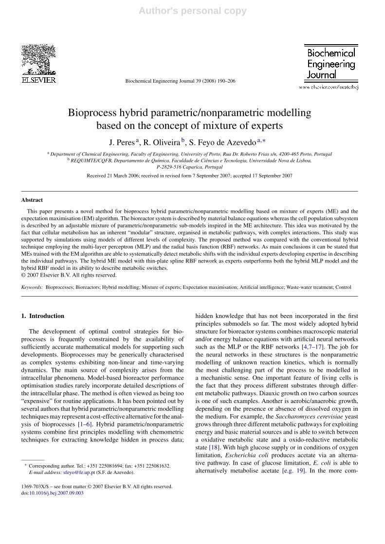
Fig. 9. Results obtained with the hybrid ME model with 2 MLP experts (204 parameters) for the test partition: (a–h) concentrations: measured values (◦), estimatedvalues (—). (i) Gaussian gating network outputs: g1 (- - -), g2 (—) vs. concentrations of SO2 ,(◦).



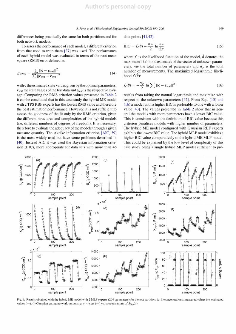
dict the biomass concentration values. The hybrid ME modelwith 2 TPS RBF experts has the highest BIC. Therefore, in thiscase study, the hybrid ME model configured with 2 TPS RBFexperts is preferable in terms of model prediction and complex-ity. The modelling results for the best three hybrid models forthe test partition are presented in Figs. 5(a)–7(a). These plotsare very similar in accordance with the previous analysis. Tovisualise the performance of the models the measured data ver-sus the estimated values from the hybrid models considered arepresented in Figs. 5(c)–7(c). These plots, just confirms the previ-ous results. Figs. 5(b) and 6(b) demonstrates again the capacityof the hybrid ME model of detecting the switch between thetwo metabolic states. The switch occurs for values of SG around0.09 g/L. Figs. 5(d) and 6(d) demonstrates the ability of eachexpert of developing expertise in describing one or the othermetabolic state on a specific part of the input space.

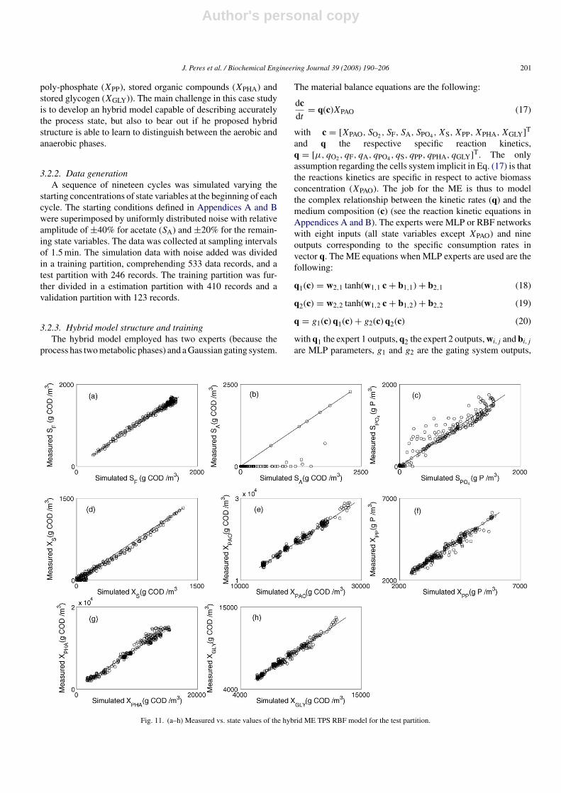
3.2. Case study B: activated sludge processes

3.2.1. Process descriptionIn this case study, a much more complex wastewater phos-

phorus removal process by activated sludge is addressed. Thestudy was supported by the activated sludge model number 2d

(ASM2d) described in [20]. The ASM2d model is a complexmorphologically and intracellularly structured model account-ing for the existence of three types of organisms. In this work,the model was simplified for aerobic phosphorus accumulatingorganisms (PAO) only. PAOs are facultative aerobic organismswith the capacity of adapting the metabolism for aerobic oranaerobic conditions. The wastewater treatment process is con-ducted in a sequencing batch reactor (SBR) operated throughrepeated batch cycles. Each SBR cycle has two main reactionphases (the other phases such as settling, medium withdrawingand replenishing with fresh medium are not relevant for thisstudy). The first phase is the anaerobiose taking a total timeof 40 min per cycle. This phase is immediately followed bythe aerobiose that takes more 20 min per cycle. The transitionbetween the anaerobiose and aerobiose is controlled by the aer-ation rate. The SBR model equations and respective parametersare presented in Appendices A and B. It should be noted that theproblem addressed here is much more complex than the problemof case study A. The process state is defined by 6 extracellu-lar state variables (concentrations of biomass (XPAO), dissolvedoxygen (SO2 ), readily biodegradable substrate (SF), acetate (SA),phosphate (SPO4 ) and slowly biodegradable substrate (XS)) andthe concentrations of 3 compounds stored intracellularly (stored

Fig. 10. Results obtained with the hybrid Gaussian RBF model (261 parameters) for the test partition: (a–h) concentrations: measured values (◦), estimated values(—).



poly-phosphate (XPP), stored organic compounds (XPHA) andstored glycogen (XGLY)). The main challenge in this case studyis to develop an hybrid model capable of describing accuratelythe process state, but also to bear out if he proposed hybridstructure is able to learn to distinguish between the aerobic andanaerobic phases.

3.2.2. Data generationA sequence of nineteen cycles was simulated varying the

starting concentrations of state variables at the beginning of eachcycle. The starting conditions defined in Appendices A and Bwere superimposed by uniformly distributed noise with relativeamplitude of ±40% for acetate (SA) and ±20% for the remain-ing state variables. The data was collected at sampling intervalsof 1.5 min. The simulation data with noise added was dividedin a training partition, comprehending 533 data records, and atest partition with 246 records. The training partition was fur-ther divided in a estimation partition with 410 records and avalidation partition with 123 records.

3.2.3. Hybrid model structure and trainingThe hybrid model employed has two experts (because the

process has two metabolic phases) and a Gaussian gating system.

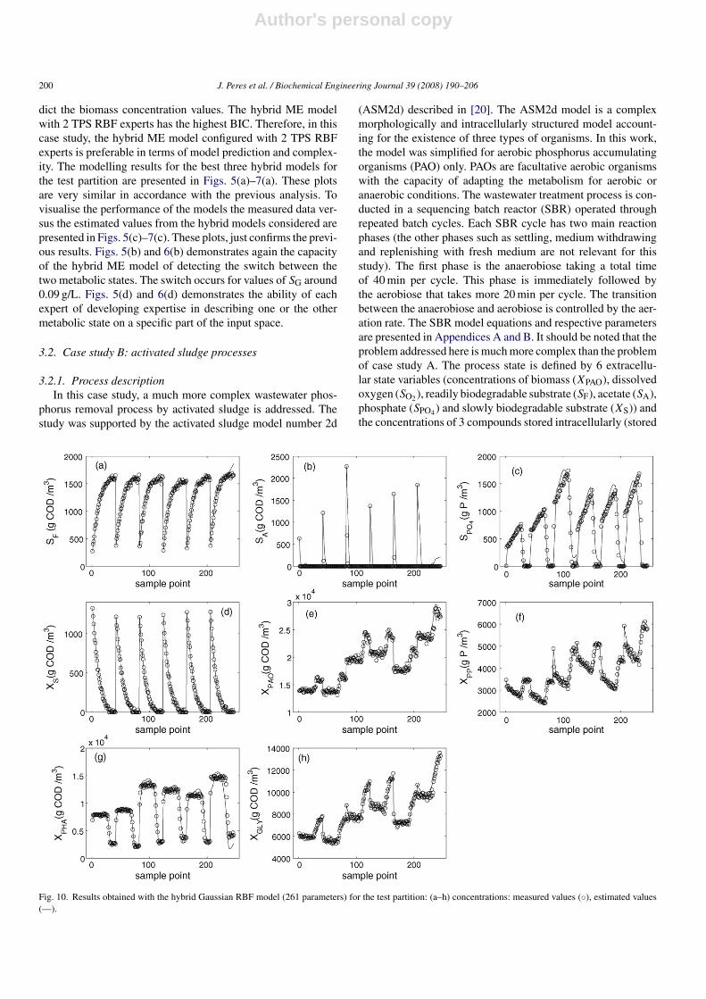
The material balance equations are the following:

dcdt

= q(c)XPAO (17)

with c = [XPAO, SO2 , SF, SA, SPO4 , XS, XPP, XPHA, XGLY]T

and q the respective specific reaction kinetics,q = [μ, qO2 , qF, qA, qPO4 , qS, qPP, qPHA, qGLY]T. The onlyassumption regarding the cells system implicit in Eq. (17) is thatthe reactions kinetics are specific in respect to active biomassconcentration (XPAO). The job for the ME is thus to modelthe complex relationship between the kinetic rates (q) and themedium composition (c) (see the reaction kinetic equations inAppendices A and B). The experts were MLP or RBF networkswith eight inputs (all state variables except XPAO) and nineoutputs corresponding to the specific consumption rates invector q. The ME equations when MLP experts are used are thefollowing:

q1(c) = w2,1 tanh(w1,1 c + b1,1) + b2,1 (18)

q2(c) = w2,2 tanh(w1,2 c + b1,2) + b2,2 (19)

q = g1(c) q1(c) + g2(c) q2(c) (20)

with q1 the expert 1 outputs, q2 the expert 2 outputs, wi,j and bi,j

are MLP parameters, g1 and g2 are the gating system outputs,

Fig. 11. (a–h) Measured vs. state values of the hybrid ME TPS RBF model for the test partition.



which are scalar quantities defining the relative contribution ofexpert 1 and 2 for the evaluation of the specific reaction kineticsq. The gating system has only one input, the concentration ofdissolved oxygen. The Gaussian gating system (see Eqs. (5)and (6)) with diagonal covariances matrix was adopted for thisstudy. The training method employed was the EM algorithm asdescribed in Section 2.3 and the parameters were identified bycross validation.

3.2.4. Model selectionAn thorough study was performed with the objective of com-

paring the hybrid model employing the ME network with twoexperts (a model that is a compromise between local and globalmodels) with the hybrid model employing the MLP network (aglobal model) or a RBF network (a local model). The optimalneural network configuration was determined by varying thenumber of hidden nodes for all ME, MLP or RBF models. Thetraining was repeated 30 times with different starting parame-ters. The experts parameters were initialised by random selectionfrom a zero mean, unit variance isotropic Gaussian where thevariance is scaled by the number of hidden or output units asappropriate [27]. The gating parameters were initialised by thekmeans algorithm applied to the gating input. The selected finalsolution was that having the lowest validation error among the

30 trials. The best configuration for all the models consideredare summarized on the first three columns of Table 3.

3.2.5. Modelling the process stateThe performance of each hybrid model was again evaluated

in terms of the root mean square (RMS) error over a test partitionas defined in the previous case study (Eq. (14)). Comparing theRMS criterion values presented in Table 3 it can be concludedthat in this study the hybrid ME model configured with 2 TPSRBF experts gives the best estimation performance. However,it is not sufficient to assess the goodness of the fit only withthe RMS criterion, given the different structures and complexi-ties of the two hybrid models (i.e. different numbers of degreesof freedom). Again, the model selection criterion used was theBayesian information criterion (BIC). The values presented inTable 3 shows that in contrast with the case A.3 the hybrid MEMLP model has a higher BIC value than the hybrid single MLPmodel. This result is in accordance with the greater level of com-plexity of this case study. Albeit the power of MLP networks formodelling nonlinear functions they have problems in describingdiscontinuities. The hybrid ME model configured with 2 TPSRBF experts has a BIC value much higher than that obtainedfor the other hybrid models considered. The capacity of the MEstructure of dividing the input space along with TPS RBFs capac-

Fig. 12. (a–h) Measured vs. state values of the hybrid ME MLP model for the test partition.



Fig. 13. (a–h) Measured vs. state values of the hybrid RBF Gaussian model for the test partition.

ity of learning local mappings seems more suitable for processeswith discontinuities. Therefore, it can be concluded that in thiscase study, the hybrid ME model configured with 2 TPS RBFexperts outperformed the hybrid single models in terms of modelprediction and complexity.

The modelling results for the test partition for those threehybrid models that has a greater BIC value are presented inFigs. 8(a–h)–10 (a–h). To visualise the performance of the mod-els the measured data versus the estimated values for the verysame hybrid models are presented in Figs. 11–13 . All the hybridmodels has difficulties in describing SA concentration. Anotherstate value not very well described is the SPO4 concentrationalthough the hybrid ME models showed an higher performance.It is evident that the estimated XPHA state value is betterdescribed by the hybrid ME TPS RBF model. Both these vari-ables, SPO4 and XPHA, has in common an abrupt switch betweenthe metabolic states so the advantage of using the hybrid MEmodels are better noticed. All the other state variables seems tobe better described by the hybrid ME models except the XS statevalues that are slightly enhanced by the single hybrid model.

3.2.6. Switch between aerobiose and anaerobioseAn important and most interesting feature of the ME was

observed: the ME network was able to detect the switch betweenthe anaerobiose and aerobiose as illustrated in Figs. 8(i) and 9(i)

and , and the experts developed expertise in modelling the kinet-ics of the one or the other metabolic state. The switch betweenthe experts occurs precisely at 0.66 h in the transition betweenthe anaerobiose and aerobiose. It has succeeded in all batches,either in training or validation batches. This feature was repeat-edly observed in several other tests with other processes (nottreated in this work).

4. Conclusions

The main objective of this work was to develop a bioprocesshybrid modelling method combining material balance equationswith modular neural network architectures for modelling cellsreaction kinetics. This idea was motivated by the fact that themetabolism of cells consists of a highly complex modular net-work of metabolic pathways. Two case studies of different levelsof complexity were considered. First, a culture of S. cerevisiaewas analysed using both data from simulation models and datafrom a set of experimental batches; subsequently a wastewatertreatment process was studied using data from simulations. Themain conclusions to be taken from this study are the following:

• the hybrid mixture of experts (ME) model, if trained with theexpectation maximisation algorithm, is able to detect differentpathways without breakdown;



• the hybrid ME model exhibited a better performance than thehybrid single model in both case studies however on the morecomplex case study such as a wastewater phosphorus removalprocess by activated sludge the difference were more evident;

• the hybrid ME TPS RBF model achieved the best predictionperformance in opposition to the hybrid ME MLP model;

• the ME architecture has the additional advantage that thesmall experts employed developed individually the expertisein describing the individual metabolic pathways;

• the ME networks are able to describe more accurately thekinetics around the metabolic switches.

In the context of hybrid modelling, modular mixture ofexperts represent a more structured description of cellular kinet-ics and thus may represent an advance in the extraction ofinformation from experimental data, yielding more accuratemodels with better generalisation properties. This technique mayconstitute a powerful methodology for biosystems identificationif connected with metabolic pathway analysis [44].

Acknowledgement

The authors acknowledge Fundacao para a Ciencia e Tecnolo-gia (FCT) for funding (contract no. POCTI/BIO/56571/2004).

Appendix A. Case study A: bakers’ yeast fed-batchcultivation model

State variables: concentrations of biomass (X), glucose (SG),ethanol (SE), and liquid volume (V). Material balance equations:

dX

dt= (μo

G + μrG + μo

E − D)X (A.1)

dSG

dt= −

(μo

G

YoGXG

+ μrG

Y rGXG

)X − D(SG − SG0) (A.2)

dSE

dt=(

μrG

Y rGXE

− μoE

YoEXE

)X − DSE (A.3)

dV

dt= DV = F (A.4)

Initial conditions—Example 1: B i: X(0) (g/L), SG(0) (g/L),SE(0) (g/L), V (0) (L), F (L/h), SG (g/L). B1: 1.20, 1.46, 2.27,2.5, 0.12, 50; B2: 1.54, 0.29, 2.90, 2.5, 0.15, 100; B3: 0.38, 1.53,1.95, 2.5, 0.15, 50; B4: 1.46, 0.00, 1.84, 2.5, 0.15, 25; B5: 0.23,3.13, 0.72, 2.5, 0.05, 10; B6: 0.25, 2.98, 0.64, 2.5, 0.10, 25.

Initial conditions–Example 3: 1 ≤ X(0) ≤ 2 g/L, 1 ≤SG(0) ≤ 2 g/L, SE(0) = 1 g/L, V (0) = 1 L, 1 ≤ F ≤ 2 L/h,SG0 = 50 g/L.

Kinetic rates:

qG = qG maxSG

KG + SG(A.5)

Aerobic metabolic state:

μoG = YoG

XGqG (A.6)

μrG = 0 (A.7)

μoE= min

(μE max

E

KE + E

Ki

Ki + SG, YoE

XO

(qo max−qG

YoGXG

YoGXO

))

(A.8)

Fermentative metabolic state:

μoG = YoG

XOqo max (A.9)

μrG = Y rG

XG

(qG − qo max

YoGXO

YoGXG

)(A.10)

μoE = 0 (A.11)

Switch between metabolic states:

• if qG ≤ qo maxYoGXO/YoG

XG⇒ respirative metabolic state (Eqs.(A.6)–(A.8))

• else if qG > qo maxYoGXO/YoG

XG⇒ fermentative metabolic state(Eqs. (A.9)–(A.11))

S. cerevisiae model parameters (taken from [18]):Kinetic parameters: qG max = 3.5 g gluc/(g cell × h), KG =

0.2 g/L, μE max = 0.17 h−1, KE = 0.1 g/L, qo max = 0.256 g O2/(g cell × h), Ko = 0.1 mg/L, Ki = 0.1 g/L.

Stoichiometric yields: YoGXG(k−1

1 ) = 0.49, Y rGXG(k−1

2 ) = 0.05,YoE

XE(k−14 ) = 0.72, YoG

XO(k−15 ) = 1.2, Y rG

XE(k−13 ) = 0.1,

YoEXO(k−1

6 ) = 0.64.

Appendix B. Case study B: simplified activated sludgemodel

State variables: concentrations of dissolved oxygen (SO2 ),readily biodegradable substrate (SF), acetate (SA), ammonium(SNH4 ), phosphate (SPO4 ), inert, non-biodegradable organics(SI), bicarbonate alkalinity (SALK), slowly biodegradable sub-strate (XS), biomass (XPAO), stored poly-phosphate (XPP),stored organic compounds (XPHA) and stored glycogen (XGLY).

Material balance equations 1:

dSO2

dt=(

1

YOPHA

− 1

)r22 − 1

YOPP

r23

+(

1 − 1

YOGLY

)r24 − r25 (B.1)

dSF

dt= (1 − fSI)(r1 + r3) (B.2)

dSA

dt= −r20 (B.3)

1 SNH4 , SALK, SI are assumed to be constant and hence the correspondingderivatives are zero.



dSPO4

dt= YPO4 r20 + r21 − 0.0144 r22 − 0.9955 r23

+ 0.0180 r24 + 0.02 r25 (B.4)

dXS

dt= −r1 − r3 (B.5)

dXPAO

dt= 1

YOPHA

r22 − 1

YOPP

r23 − 1

YOGLY

r24 − r25 (B.6)

dXPP

dt= −YPO4 r20 − r21 + r23 (B.7)

dXPHA

dt= YPHA r20 − r22 (B.8)

dXGLY

dt= (1 − YPHA) r20 + r24 (B.9)

SO2 (0) = 0 g O2/m3, SF(0) = 300 g COD/m3, SA(0) =1890 g COD/m3, SNH4 (0) = 12.6 g N/m3, SPO4 (0) = 9 gP/m3,SI(0) = 300 g COD/m3, SALK(0) = 50 g HCO3

−/m3, XS(0) =1250 g COD/m3, XPAO(0) = 18, 000 g COD/m3, XPP(0) =4500 g P/m3, XPHA(0) = 9000 g COD/m3, XGLY(0) =8100 g COD/m3.

Kinetic equations:

r1 = khfS

KX + fS

SO2

KLO2

+ SO2

XPAO (B.10)

r3 = ηLfe kh

fS

KX + fS

KLO2

KLO2

+ SO2

XPAO (B.11)

r20 = qmaxs,AN

SA

KA + SA

f maxPHA − fPHA

KfPHA + f maxPHA − fPHA

× XGLY

KGLY + XGLY

XPP

KPP + XPPXPAO (B.12)

r21 = mANKO2

KO2 + SO2

XPP

KPP + XPPXPAO (B.13)

r22 = kPHAfPHA

KfPHA + fPHA

SO2

KO2 + SO2

SNH4

KNH4 + SNH4

× SPO4

KP + SPO4

SALK

KALK + SALKXPAO (B.14)

r23 = kPPXPAO

XPP

SPO4

KPO4 + SPO4

SO2

gPPKO2 + SO2

× f maxPP − fPP

KfPP + f maxPP − fPP

XPHA

KPHA + XPHAXPAO (B.15)

r24 = kGLYXPHA

XGLY

SO2

KO2 + SO2

f maxGLY − fGLY

KfGLY + f maxGLY − fGLY

× XPHA

KPHA + XPHAXPAO (B.16)

r25 = mO2

SO2

KO2 + SO2

XPAO (B.17)

fi = Xi

XPAO(B.18)

Stoichiometric parameters: fSI = 0 (g COD/g COD), YOPHA =

1.39 (g COD/g COD), YPO4 = 0.35 (g P/g COD), YOGLY = 1.11

(g COD/g COD) YPHA = 1.50 (g COD/g COD), YOPP = 4.42

(g P/g COD).Kinetic parameters: kh = 3.0 (g COD/g COD d), KL

O2=

0.20 (g O2/m3), ηLfe = 0.2, KX = 0.1 (g COD/g COD),

qmax ,APs,AN = 8.0 (g COD/g COD d), kPHA = 5.51 (g COD/

g COD d), mAN = 0.05 (g P/g COD d), kPP = 0.10(g P/g COD d), kGLY = 0.93 (g COD/g COD d), gPP = 0.22,mO2 = 0.06 (g O2/g COD d), KP = 1.00 (g P/m3), KA = 4.00(g COD/m3), KfPHA = 0.20 (g COD/g COD), KO2 = 0.20(g O2/m3), KPO4 = 0.02 (g P/m3), KNH4 = 0.05 (g N/m3),f max

PP = 0.35 (g P/g COD), f maxPHA = 0.05 (g COD/g COD),

f maxGLY = 0.50 (g COD/g COD), KPP = 0.01 (g P/m3),

KPHA = 0.01 (g COD/m3), KGLY = 0.01 (g COD/m3),KfGLY = 0.01 (g COD/g COD), KfPP = 0.01 (g P/g COD),KALK = 0.01 (mol HCO3

−/m3).

References

[1] J. Schubert, R. Simutis, M. Dors, I. Havlik, A. Lubbert, Hybrid modeling ofyeast production processescombination of a-priori knowledge on differentlevels of sophistication, Chem. Eng. Technol. 17 (1) (1994) 10–20.

[2] H. Preusting, J. Noordover, R. Simutis, A. Lubbert, The use of hybrid mod-elling for the optimization of the penicillin fermentation process, Chimia50 (9) (1996) 416–417.

[3] R. Simutis, R. Oliveira, M. Manikowski, S.F. de Azevedo, A. Lubbert, Howto increase the performance of models for process optimization and control,J. Biotechnol. 59 (1–2) (1997) 73–89.

[4] H.J.L. van Can, H.A.B. teBraake, S. Dubbelman, C. Hellinga, K.C.A.M.Luyben, J.J. Heijnen, Understanding and applying the extrapolation prop-erties of serial gray-box models, AIChE J. 44 (5) (1998) 1071–1089.

[5] A. Tholudur, W.F. Ramirez, J.D. McMillan, Mathematical modeling andoptimization of cellulase protein production using Trichoderma reesei RL-P37, Biotechnol. Bioeng. 66 (1) (1999) 1–16.

[6] J. Peres, R. Oliveira, S.F. de Azevedo, Knowledge based modular net-works for process modelling and control, Comput. Chem. Eng. 25 (2001)783–791.

[7] D.C. Psichogios, L.H. Ungar, A hybrid neural network—1st principlesapproach to process modeling, AIChE J. 38 (10) (1992) 1499–1511.

[8] M.L. Thompson, M.A. Kramer, Modeling chemical processes using priorknowledge and neural networks, AIChE J. 40 (8) (1994) 1328–1340.

[9] G. Montague, J. Morris, Neural-network contributions in biotechnology,Trends Biotechnol. 12 (8) (1994) 312–324.

[10] S.F. de Azevedo, B. Dahm, F.R. Oliveira, Hybrid modelling of biochemicalprocesses: a comparison with the conventional approach, Comput. Chem.Eng. 21 (1997) S751–S756.

[11] H.J.L. van Can, H.A.B.T. Braake, C. Hellinga, K.C.A.M. Luyben, J.J. Hei-jnen, An efficient model development strategy for bioprocesses based onneural networks in macroscopic balances. Part II, Biotechnol. Bioeng. 62(6) (1999) 666–680.

[12] L. Chen, O. Bernard, G. Bastin, P. Angelov, Hybrid modelling of biotech-nological processes using neural networks, Control Eng. Pract. 8 (7) (2000)821–827.

[13] A. Karama, O. Bernard, A. Genovesi, D. Dochain, A. Benhammou, J.P.Steyer, Hybrid modelling of anaerobic wastewater treatment processes,Water Sci. Technol. 43 (1) (2001) 43–50.



[14] A. Karama, O. Bernard, J.L. Gouze, A. Benhammou, D. Dochain, Hybridneural modelling of an anaerobic digester with respect to biological con-straints, Water Sci. Technol. 43 (7) (2001) 1–8.

[15] A. Andr sik, A. Msz ros, S.F. de Azevedo, On-line tuning of a neural PIDcontroller based on plant hybrid modeling, Comput. Chem. Eng. 28 (8)(2004) 1499–1509.

[16] A. Teixeira, A. Cunha, J. Clemente, J. Moreira, H. Cruz, P. Alves, M.Carrondo, R. Oliveira, Modelling and optimization of a recombinant BHK-21 cultivation process using hybrid grey-box systems, J. Biotechnol. 118(3) (2005) 290–303.

[17] A. Teixeira, J. Clemente, A. Cunha, M. Carrondo, R. Oliveira,Bioprocess iterative batch-to-batch optimization based on hybrid paramet-ric/nonparametric models, Biotechnol. Progr. 22 (1) (2006) 247–258.

[18] B. Sonnleitner, O. Kappeli, Growth of Saccharomyces-cerevisiae is con-trolled by its limited respiratory capacity formulation and verification of ahypothesis, Biotechnol. Bioeng. 28 (6) (1986) 927–937.

[19] H.E. Reiling, H. Laurila, A. Fiechter, Mass-culture of escherichia-colimedium development for low and high-density cultivation ofescherichia coli-b/r in minimal and complex media, J. Biotechnol. 2 (3–4)(1985) 191–206.

[20] M. Henze, W. Gujer, T. Mino, T. Matsuo, M.C. Wentzel, G.V.R. Marais,M.C.M. Van Loosdrecht, Activated sludge model no.2d, ASM2d, WaterSci. Technol. 39 (1) (1999) 165–182.

[21] S. Haykin, Neural Networks: A Comprehensive Foundation, MacmillanCollege Publishing Company Inc., 1994.

[22] B. Eikens, M.N. Karim, Process identification with multiple neural networkmodels, Int. J. Control 72 (7–8) (1999) 576–590.

[23] R.A. Jacobs, M.I. Jordan, S.J. Nowlan, G.E. Hinton, Adaptive mixtures oflocal experts, Neural Comput. 3 (1991) 79–87.

[24] R. Oliveira, J. Peres, S.F. de Azevedo, Hybrid modelling of fermentationprocesses using artificial neural networks: a study on identification andstability, in: M. Pons, J.F.M. van Impe (Eds.), Computer Applications inBiotechnology 2004, Elsevier, 2005, pp. 195–200 (ISBN: 0-08-044251-X).

[25] J. Peres, R. Oliveira, S.F. de Azevedo, Hybrid modelling of fermentationprocesses: a study on the use of modular neural networks for modellingcells reaction kinetics, in: M. Pons, J.F.M. van Impe (Eds.), ComputerApplications in Biotechnology 2004, Elsevier, 2005, pp. 293–298 (ISBN:0-08-044251-X).

[26] D.M. Titterington, A.F.M. Smith, U.E. Makov, Analysis of Finite MixtureDistributions, Wiley, New York, 1985.

[27] C.M. Bishop, Neural Networks for Pattern Recognition, Oxford UniversityPress, 1995.

[28] V. Ramamurti, J. Ghosh, Structurally adaptive modular networks fornonstationary environments, IEEE Trans. Neural Network 10 (1) (1999)152–160.

[29] L. Xu, M.I. Jordan, G.E. Hinton, An alternative model for mixture ofexperts, in: G. Tesauro, D.S. Touretzky, T.K. Leen (Eds.), Advances inNeural Information Processing Systems, vol. 7, MIT Press, 1995, pp. 633–640.

[30] S. Haykin, Neural Networks: A Comprehensive Foundation, 2nd ed., Pren-tice Hall Inc., 1999.

[31] A.P. Dempster, N.M. Laird, D.B. Rubin, Maximum likelihood from incom-plete data via EM algorithm, J. R. Stat. Soc. B: Methodol. 39 (1) (1977)1–38.

[32] M.I. Jordan, R.A. Jacobs, Hierarchical mixtures of experts and the EMalgorithm, Neural Comput. 6 (2) (1994) 181–214.

[33] A.V. Rao, D. Miller, K. Rose, A. Gersho, Mixture of experts regressionmodeling by deterministic annealing, IEEE Trans. Signal Process. 45 (11)(1997) 2811–2820.

[34] M.I. Jordan, L. Xu, Convergence results for the EM approach to mix-tures of experts architectures, Neural Networks 8 (9) (1995) 1409–1431.

[35] M.F. Moller, A scaled conjugate-gradient algorithm for fast supervisedlearning, Neural Networks 6 (4) (1993) 525–533.

[36] D.E. Rumelhart, G.E. Hinton, R.J. Williams, Learning internal representa-tions by error propagation, in: D.E. Rumelhart, J.L. McClelland, the PDPResearch Group (Eds.), Parallel Distributed Processing: Explorations in theMicrostructure of Cognition, Vol. 1: Foundations, MIT Press, Cambridge,MA, 1986, pp. 318–362.

[37] P. Moerlan, Mixture Models for Unsupervised and Supervised Learning,PhD thesis, Computer Science Department, Swiss Federal Institute of Tech-nology at Lausanne (EPFL), 2000.

[38] J. Moody, C.J. Darken, Fast learning in networks of locally-tuned process-ing units, Neural Comput. 1 (1989) 281–294.

[39] H. Akaike, New look at statistical-model identification AC19 (6) (1974)716–723.

[40] U. Anders, O. Korn, Model selection in neural networks, Neural Networks12 (2) (1999) 309–323.

[41] T. Leonard, J. Hsu, Bayesian Methods, Cambridge University Press, NewYork, 1999.

[42] I.G. Main, T. Leonard, O. Papasouliotis, C.G. Hatton, P.G. Meredith, Oneslope or two? Detecting statistically significant breaks of slope in geophys-ical data, with application to fracture scaling relationships, Geophys. Res.Lett. 26 (18) (1999) 2801–2804.

[43] T. Seher, I.G. Main, A statistical evaluation of a ‘stress-forecast’ earth-quake, Geophys. Res. Lett. 157 (1) (2004) 187–193.

[44] S. Schuster, D. Fell, T. Dandekar, A general definition of metabolic path-ways useful for systematic organization and analysis of complex metabolicnetworks, Nat. Biotechnol. 18 (2000) 326–332.

author's personal copy -...

Documents