atomic scheduling of appliance energy consumption in residential smart grid
TRANSCRIPT

Atomic Scheduling of ApplianceEnergy Consumption in Residential
Smart Grid
Kyeong Soo (Joseph) Kim(With S. Lee, T. O. Ting@XJTLU and X.-S. Yang@Middlesex)
Department of Electrical and Electronic EngineeringXi’an Jiaotong-Liverpool University
CeSGIC 1st International Workshop onSmart Grid Technology and Data Processing
19 June 2015
1 / 55

OutlineIntroductionReview of Current Formulation of Appliance EnergyConsumption Scheduling
Atomic Scheduling of Appliance Energy ConsumptionStarting-Time-Based FormulationOptimal-Routing-Based FormulationSuccessive Convex RelaxationExamples
Numerical ResultsExperimental ParametersComparison of Bounds with True Optimal ValuesCost MinimizationPAR Minimization
Conclusions
2 / 55


Next . . .IntroductionReview of Current Formulation of Appliance EnergyConsumption Scheduling
Atomic Scheduling of Appliance Energy ConsumptionStarting-Time-Based FormulationOptimal-Routing-Based FormulationSuccessive Convex RelaxationExamples
Numerical ResultsExperimental ParametersComparison of Bounds with True Optimal ValuesCost MinimizationPAR Minimization
Conclusions
4 / 55

Autonomous Demand-Side Management inSmart Grid
Gateway(Traditional)
Electricity
Grid
Greenfield
Power
Line
Bi-Directional
Communication
Links
Power Plant
5 / 55

Scheduling of Appliance EnergyConsumption
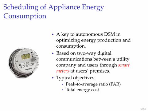
I A key to autonomous DSM inoptimizing energy production andconsumption.
I Based on two-way digitalcommunications between a utilitycompany and users through smartmeters at users’ premises.
I Typical objectivesI Peak-to-average ratio (PAR)I Total energy cost
6 / 55

Scheduling of Appliance EnergyConsumption
I A key to autonomous DSM inoptimizing energy production andconsumption.
I Based on two-way digitalcommunications between a utilitycompany and users through smartmeters at users’ premises.
I Typical objectivesI Peak-to-average ratio (PAR)I Total energy cost
6 / 55

A Question on Scheduled EnergyConsumption
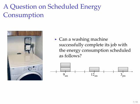
I Can a washing machinesuccessfully complete its job withthe energy consumption scheduledas follows?
7 / 55
A Question on Scheduled EnergyConsumption
I Can a washing machinesuccessfully complete its job withthe energy consumption scheduledas follows?
9am 3pm12am
7 / 55

A Question on Scheduled EnergyConsumption
I Can a washing machinesuccessfully complete its job withthe energy consumption scheduledas follows?
9am 3pm12am
or
7 / 55

A Question on Scheduled EnergyConsumption
I Can a washing machinesuccessfully complete its job withthe energy consumption scheduledas follows?
9am 3pm12am
or
9am 3pm2pm10am
7 / 55

Next . . .IntroductionReview of Current Formulation of Appliance EnergyConsumption Scheduling
Atomic Scheduling of Appliance Energy ConsumptionStarting-Time-Based FormulationOptimal-Routing-Based FormulationSuccessive Convex RelaxationExamples
Numerical ResultsExperimental ParametersComparison of Bounds with True Optimal ValuesCost MinimizationPAR Minimization
Conclusions
8 / 55

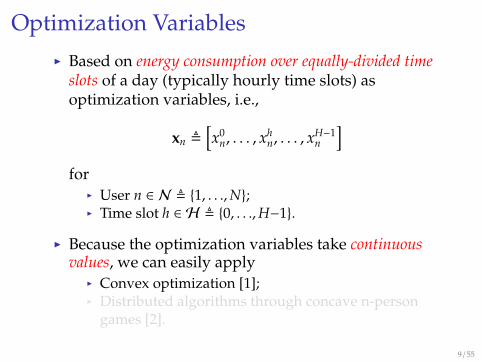
Optimization VariablesI Based on energy consumption over equally-divided time
slots of a day (typically hourly time slots) asoptimization variables, i.e.,
xn ,[x0
n, . . . , xhn, . . . , x
H−1n
]for
I User n ∈ N , {1, . . .,N};I Time slot h ∈ H , {0, . . .,H−1}.
I Because the optimization variables take continuousvalues, we can easily apply
I Convex optimization [1];I Distributed algorithms through concave n-person
games [2].
9 / 55

Feasible SetA feasible energy consumption scheduling set for user n
Xn=
{xn
∣∣∣∣∣∣ ∑h∈Hn
xhn=En, γ
minn ≤xh
n≤γmaxn , ∀h∈Hn, xh
n=0, ∀h∈H\Hn
}whereI γmin
n : Minimum energy level;I γmax
n : Maximum energy level;I En: Total daily energy consumption;I Hn: Scheduling interval defined as follows:
Hn ,{h∣∣∣h = i mod H, ∀i∈
[αn, βn
]}with αn∈[0, H−1], βn∈[1, 2H−2], and 1≤βn−αn≤H−1.
10 / 55

Optimal SchedulingThe optimal scheduling is formulated as an optimizationproblem for a given objective function φ(·) (e.g., totalenergy cost or PAR) as follows:
minimizexn∈Xn, ∀n∈N
φ (L(x))
whereI x , [x1, . . . , xN]: A vector of user energy consumption
vectors;I L(x) , [L0 (x) , . . . ,LH−1 (x)]: A vector of aggregate
loads across all users at each time slot, which aredefined as
Lh (x) ,∑n∈N
xhn.
11 / 55

Objective Functions
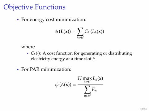
I For energy cost minimization:
φ (L(x)) =∑h∈H
Ch (Lh(x))
whereI Ch(·): A cost function for generating or distributing
electricity energy at a time slot h.
I For PAR minimization:
φ (L(x)) =
H maxh∈H
Lh(x)∑n∈N
En
12 / 55
Objective Functions
I For energy cost minimization:
φ (L(x)) =∑h∈H
Ch (Lh(x))
whereI Ch(·): A cost function for generating or distributing
electricity energy at a time slot h.
I For PAR minimization:
φ (L(x)) =
H maxh∈H
Lh(x)∑n∈N
En
12 / 55

Atomic vs. Non-Atomic Scheduling
αn,a βn,a
αn,a βn,a
Gap Gap
γminn
γmaxn
(a)
γopn (·)
γminn
γmaxn
(b)
Examples of (a) non-atomic and (b) atomic scheduling.I γmin
n : Minimum energy levelI γmax
n : Maximum energy levelI γop
n (·): Operating energy level
13 / 55

Non-Atomic Scheduling Example
Appliance 1
Appliance 2
Scheduled
Consumption?
14 / 55

Non-Atomic Scheduling Example: Case 1
Appliance 1
Appliance 2
Scheduled
Consumption
15 / 55
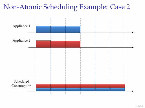
Non-Atomic Scheduling Example: Case 2
Appliance 1
Appliance 2
Scheduled
Consumption
16 / 55

Non-Atomic Scheduling Example: Case 3
Appliance 1
Appliance 2
Scheduled
Consumption
17 / 55

Next . . .IntroductionReview of Current Formulation of Appliance EnergyConsumption Scheduling
Atomic Scheduling of Appliance Energy ConsumptionStarting-Time-Based FormulationOptimal-Routing-Based FormulationSuccessive Convex RelaxationExamples
Numerical ResultsExperimental ParametersComparison of Bounds with True Optimal ValuesCost MinimizationPAR Minimization
Conclusions
18 / 55

Overview of Atomic Scheduling ProblemFormulation & Solution
Starting-Time-BasedFormulation
Optimal-Routing-BasedFormulation
Convex Relaxation
Successive ConvexRelaxation withFractional-Value
Dropping
ConvexOptimization
(Feasible Upper Bound)
CombinatorialOptimization
Boolean-ConvexOptmization
ConvexOptmization
(Lower Bound)
19 / 55

Next . . .IntroductionReview of Current Formulation of Appliance EnergyConsumption Scheduling
Atomic Scheduling of Appliance Energy ConsumptionStarting-Time-Based FormulationOptimal-Routing-Based FormulationSuccessive Convex RelaxationExamples
Numerical ResultsExperimental ParametersComparison of Bounds with True Optimal ValuesCost MinimizationPAR Minimization
Conclusions
20 / 55

Starting-Time-Based FormulationI Optimization variables:
s , [s1, . . . , sN]
I A feasible set for user n:
Sn ,{sn
∣∣∣sn = i mod H, ∀i∈[αn, βn−δn+1]}
I Aggregate load across all users at each time slot h:
Lh(s) ,∑n∈N
γopn ((h − sn) mod H) IRn(sn)(h)
whereI IRn(sn)(h): An indicator function for a set Rn(sn).I Rn(sn): A range of user n’s appliance operation for sn
defined as follows:
Rn(sn) ,{h∣∣∣h = i mod H, ∀i∈ [sn, sn + δn − 1]
}21 / 55

Issues with Starting-Time-Based Formulation
I Because the feasible set is now discrete, we have toevaluate the objective function for all the elements in thefeasible set.
I The optimization by direct enumeration becomesimpractical for large N and H.
I When N=100 and H=24 with the worst case scenarioof αn=0, βn=23, and δn=1 for all n∈N , we need toevaluate the objective function 24100 times, which ison the order of 10138 times!
22 / 55

Next . . .IntroductionReview of Current Formulation of Appliance EnergyConsumption Scheduling
Atomic Scheduling of Appliance Energy ConsumptionStarting-Time-Based FormulationOptimal-Routing-Based FormulationSuccessive Convex RelaxationExamples
Numerical ResultsExperimental ParametersComparison of Bounds with True Optimal ValuesCost MinimizationPAR Minimization
Conclusions
23 / 55

Why London Eye?
Does the London Eyehave something todo with the atomicscheduling?
24 / 55

A Network, A Path, and Links
S
D
0 12
3
4
5
6
7
8
9
10111213
14
15
16
17
18
19
20
21
2223
l9,10l10,11
l11,12
p9,3
A network connectingthe source (S) and thedestination (D)through 24intermediate nodeswith a path (p9,3) andits constituent links(l9,10, l10,11, and l11,12).
25 / 55
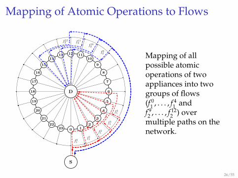
Mapping of Atomic Operations to Flows
0 12
3
4
5
6
7
8
9
10111213
14
15
16
17
18
19
20
21
2223
f01
f11
f21
f31
f41
f92
f102
f112f12
2
S
D
Mapping of allpossible atomicoperations of twoappliances into twogroups of flows(f 0
1 , . . . , f41 and
f 92 , . . . , f
122 ) over
multiple paths on thenetwork.
26 / 55

Optimization Variables and Feasible SetI Optimization variables: Flow configurations of all users
defined asf ,
[f 1, . . . , f n, . . . , f N
]where
f n ,[f 0n , . . . , f
H−1n
].
I A feasible atomic energy consumption scheduling setfor user n:
Fn =
{fn
∣∣∣∣∣∣∑s∈Sn
f sn=1, f s
n∈ {0, 1} , ∀s∈Sn, f sn=0, ∀s∈H\Sn
}where Sn is the feasible set of starting times for user nthat is already defined in starting-time-basedformulation.
27 / 55

Atomic Optimal SchedulingI Atomic optimal scheduling for an objective function
of φ(·) is formulated as follows:
minimizefn∈Fn,∀n∈N
φ (L (f)) .
whereI L (f), [L0 (f) , . . . ,LH−1 (f)]: A vector of aggregate loads
across all flows at each time slot, which are defined as
Lh(f) ,∑n∈N
γopn ((h−s) modH)
∑s∈Sn
f snIRn(s)(h)
.I Note that for a convex objective function, this
problem becomes a Boolean-convex problem, since theoptimization variable f s
n is restricted to only 0 or 1.28 / 55

Next . . .IntroductionReview of Current Formulation of Appliance EnergyConsumption Scheduling
Atomic Scheduling of Appliance Energy ConsumptionStarting-Time-Based FormulationOptimal-Routing-Based FormulationSuccessive Convex RelaxationExamples
Numerical ResultsExperimental ParametersComparison of Bounds with True Optimal ValuesCost MinimizationPAR Minimization
Conclusions
29 / 55

Relaxed Atomic Optimal SchedulingI We can relax the atomic optimal scheduling problem
by replacing f sn∈ {0, 1}with 0≤f s
n≤1 in constraints asfollows:
minimizefn∈F̂n,∀n∈N
φ (L (f))
where
F̂n =
{fn
∣∣∣∣∣∣∑s∈Sn
f sn=1, 0 ≤ f s
n ≤ 1, ∀s∈Sn, f sn=0, ∀s∈H\Sn
}.
I For a convex objective function, this problembecomes convex because F̂n is now a convex set. Itcan be solved efficiently, for instance, using thewell-known interior-point method [1].
30 / 55

Relaxed vs. Original Scheduling Problems
I The relaxed atomic optimal scheduling problem isnot equivalent to the original problem.
I The elements of the optimal solution from the relaxedproblem can take fractional values (e.g., 0.75).
I The optimal solution of the relaxed problem,however, provides a lower bound on the optimalsolution of the original problem.
I The feasible set for the relaxed problem contains thefeasible set for the original problem.
31 / 55

Successive Convex Relaxation
First, we solve the relaxed convex optimization problem.Then, carry out the following procedures:
1. Identify the maximum element of each user flowconfiguration vector (i.e., corresponding to f n) andexclude them in the following procedures.
2. Arrange in ascending order the remaining elementsthat are less than 1.
3. Drop the smallest element and add a zero constraintfor it.
32 / 55

Successive Convex Relaxation (Cont.)
4. For the rest of the elements, drop them and add zeroconstraints from the smallest element up to ND
elements in total (including the one in step 3) as far asthe element is less than a dropping threshold (θD);otherwise, stop dropping and go to the next step.
5. If there remains only one nonzero element per userflow configuration vector, stop here (a solutionfound); otherwise, solve a new relaxed convexoptimization problem with augmented constraintsand repeat the whole procedure from step 1.
33 / 55

Successive Convex Relaxation: An ExampleConsider a simple case of N=2, H=4, and ND = 1.I Initial condition:
f = [ 0.25 0.25 0.25 0.25 | 0.3 0.2 0.25 0.25 ]
I After 1st step:
f = [ 0.0 0.2 0.3 0.5 | 0.7 0.0 0.2 0.1 ]
I After 2nd step:
f = [ 0.0 0.0 0.2 0.8 | 0.9 0.0 0.1 0.0 ]
Stop here. Solution found!
34 / 55

Next . . .IntroductionReview of Current Formulation of Appliance EnergyConsumption Scheduling
Atomic Scheduling of Appliance Energy ConsumptionStarting-Time-Based FormulationOptimal-Routing-Based FormulationSuccessive Convex RelaxationExamples
Numerical ResultsExperimental ParametersComparison of Bounds with True Optimal ValuesCost MinimizationPAR Minimization
Conclusions
35 / 55

Energy Cost and PAR Minimization
I Energy cost minization
minimizefn∈F̂n,∀n∈N
∑h∈H
Ch (Lh(f)) .
I PAR minimization
minimizeΓ,fn∈F̂n,∀n∈N
Γ
subject to Γ ≥ Lh(f), ∀h ∈ H .
I Note that PAR minimization is formulated as a relaxedlinear program by introducing a new auxiliary variableΓ.
36 / 55

Energy Cost and PAR Minimization
I Energy cost minization
minimizefn∈F̂n,∀n∈N
∑h∈H
Ch (Lh(f)) .
I PAR minimization
minimizeΓ,fn∈F̂n,∀n∈N
Γ
subject to Γ ≥ Lh(f), ∀h ∈ H .
I Note that PAR minimization is formulated as a relaxedlinear program by introducing a new auxiliary variableΓ.
36 / 55

Energy Cost and PAR Minimization
I Energy cost minization
minimizefn∈F̂n,∀n∈N
∑h∈H
Ch (Lh(f)) .
I PAR minimization
minimizeΓ,fn∈F̂n,∀n∈N
Γ
subject to Γ ≥ Lh(f), ∀h ∈ H .
I Note that PAR minimization is formulated as a relaxedlinear program by introducing a new auxiliary variableΓ.
36 / 55

Next . . .IntroductionReview of Current Formulation of Appliance EnergyConsumption Scheduling
Atomic Scheduling of Appliance Energy ConsumptionStarting-Time-Based FormulationOptimal-Routing-Based FormulationSuccessive Convex RelaxationExamples
Numerical ResultsExperimental ParametersComparison of Bounds with True Optimal ValuesCost MinimizationPAR Minimization
Conclusions
37 / 55

Next . . .IntroductionReview of Current Formulation of Appliance EnergyConsumption Scheduling
Atomic Scheduling of Appliance Energy ConsumptionStarting-Time-Based FormulationOptimal-Routing-Based FormulationSuccessive Convex RelaxationExamples
Numerical ResultsExperimental ParametersComparison of Bounds with True Optimal ValuesCost MinimizationPAR Minimization
Conclusions
38 / 55

Appliance Energy ConsumptionRequirements
Appliance Parametersα [h] β [h] γop [kWh] δ [h]
Dish Washer 0 23 0.7200 2Washing Machine 0 23 0.4967 3(Energy Star)Washing Machine 0 23 0.6467 3(Regular)
Clothes Dryer 0 23 0.6250 4PHEV1 222 292 3.3000 3
1 Plug-in hybrid electric vehicle.2 Scheduling interval of 10 PM–5 AM.
I An appliance is randomly selected for each user.I Constant operating energy levels (γop) are assumed.
39 / 55

Hourly Cost Function
We assume a simple quadratic hourly cost function as in[3], i.e.,
Ch (Lh) = ahL2h [cent]
where
ah =
{0.2 if h ∈ [0, 7],0.3 if h ∈ [8, 23].
40 / 55

Hourly Cost Function
We assume a simple quadratic hourly cost function as in[3], i.e.,
Ch (Lh) = ahL2h [cent]
where
ah =
{0.2 if h ∈ [0, 7],0.3 if h ∈ [8, 23].
40 / 55

Performance Measures and Parameter Values
I Performance measuresI Lower bound: LBI Upper bound with ND: UB (ND)I Gap: G , UB(D) − LBI Number of iterations
I Parameter values for successive convex relaxationI Dropping threshold (θD): 0.1I Maximum number of fractional-valued elements that
can be dropped per iteration (ND): 1, 2, 5, 10
41 / 55

Next . . .IntroductionReview of Current Formulation of Appliance EnergyConsumption Scheduling
Atomic Scheduling of Appliance Energy ConsumptionStarting-Time-Based FormulationOptimal-Routing-Based FormulationSuccessive Convex RelaxationExamples
Numerical ResultsExperimental ParametersComparison of Bounds with True Optimal ValuesCost MinimizationPAR Minimization
Conclusions
42 / 55

Upper/Lower Bounds vs. True OptimalValues: Cost Minimization
2 3 4 5 6 7 8 9 100
5 · 10−2
0.1
0.15
0.2
0.25
0.3
0.35
N
Energy
Cost[U
SD]
LB
GO
UB(1)
UB(2)
UB(5)
UB(10)
43 / 55

Upper/Lower Bounds vs. True OptimalValues: PAR Minimization
2 3 4 5 6 7 8 9 100
1
2
3
4
5
6
7
8
9
10
N
PAR
inAgg
rega
tedLoad
LB
GO
UB(1)
UB(2)
UB(5)
UB(10)
44 / 55

Next . . .IntroductionReview of Current Formulation of Appliance EnergyConsumption Scheduling
Atomic Scheduling of Appliance Energy ConsumptionStarting-Time-Based FormulationOptimal-Routing-Based FormulationSuccessive Convex RelaxationExamples
Numerical ResultsExperimental ParametersComparison of Bounds with True Optimal ValuesCost MinimizationPAR Minimization
Conclusions
45 / 55

Cost Minimization: Upper/Lower Bounds
2 10 20 30 40 500
1
2
3
4
5
N
Energy
Cost[U
SD]
LBUB(1)UB(2)UB(5)UB(10)
46 / 55

Cost Minimization: Gaps
2 10 20 30 40 500
1
2
3
4
5
6
7×10⁻²
N
Gap
[USD]
UB(1)−LBUB(2)−LBUB(5)−LBUB(10)−LB
47 / 55

Cost Minimization: Number of Iterations
2 10 20 30 40 500
200
400
600
800
1,000
N
Number
ofIterations
UB(1)UB(2)UB(5)UB(10)
48 / 55

Next . . .IntroductionReview of Current Formulation of Appliance EnergyConsumption Scheduling
Atomic Scheduling of Appliance Energy ConsumptionStarting-Time-Based FormulationOptimal-Routing-Based FormulationSuccessive Convex RelaxationExamples
Numerical ResultsExperimental ParametersComparison of Bounds with True Optimal ValuesCost MinimizationPAR Minimization
Conclusions
49 / 55

Par Minimization: Upper/Lower Bounds
2 10 20 30 40 500
5
10
15
20
25
N
PAR
inAggregatedLoad
LBUB(1)UB(2)UB(5)UB(10)
50 / 55

Par Minimization: Gaps
2 10 20 30 40 500
1
2
3
N
Gap
UB(1)−LBUB(2)−LBUB(5)−LBUB(10)−LB
51 / 55

Par Minimization: Number of Iterations
2 10 20 30 40 500
200
400
600
800
1,000
N
Number
ofIterations
UB(1)UB(2)UB(5)UB(10)
52 / 55

Next . . .IntroductionReview of Current Formulation of Appliance EnergyConsumption Scheduling
Atomic Scheduling of Appliance Energy ConsumptionStarting-Time-Based FormulationOptimal-Routing-Based FormulationSuccessive Convex RelaxationExamples
Numerical ResultsExperimental ParametersComparison of Bounds with True Optimal ValuesCost MinimizationPAR Minimization
Conclusions
53 / 55

ConclusionsI We have provided a new formulation of appliance energy
consumption scheduling based on the optimal routingframework.
I It guarantees the atomicity of resulting scheduledenergy consumption.
I We have also provided an efficient solution techniquebased on successive convex relaxation for aBoolean-convex problem resulting from a convexobjective function.
I It enables us to carry out systematic analysis of theoriginal problem with both upper and lower bounds.
I Possible extensions to the current work includeI Distributed atomic energy consumption scheduling;I Advanced techniques refining the feasible region at
each iterative step to reduce the total number ofiterations.
54 / 55

References I
S. Boyd and L. Vandenberghe, Convex optimization.Cambridge, U.K.: Cambridge Universtiy Press, 2004.
J. B. Rosen, “Existence and uniqueness of equilibriumfor concave N-person games,” Econometrica, vol. 33,no. 3, pp. 520–534, Jul. 1965.
A.-H. Mohsenian-Rad, V. W. S. Wong, J. Jatskevich,R. Schober, and A. Leon-Garcia, “Autonomousdemand-side management based on game-theoreticenergy consumption scheduling for the future smartgrid,” IEEE Trans. Smart Grid, vol. 1, no. 3, pp.320–331, Dec. 2010.
55 / 55