atomic orbitals: explained and derived by energy wave ... · 1 atomic orbitals: explained and...
TRANSCRIPT
1
Atomic Orbitals: Explained and Derived by Energy Wave Equations
Jeff Yee,1,2 Yingbo Zhu,1,3 Guofu Zhou1
1 Electronic Paper Display Institute, South China Academy of Advanced Optoelectronics, South China Normal University, Higher Education Mega Center, Guangzhou 510006 CHINA
2 ZTE USA Inc, Milpitas, California, 95035 USA 3 China Telecom Imusic Ltd, Guangzhou, Guangdong, 510081 CHINA
Email: [email protected]
August 13, 2017
Summary
Physics separates the study of motion into two branches based on the size of the object in motion: classical mechanics for objects typically larger than an atom and quantum mechanics for atoms and subatomic particles. Quantum mechanics surfaced, in part, to solve the failure of classical mechanics’ explanation of the electron and its atomic orbital. Early attempts to explain the electron’s motion using classical methods failed because of assumptions that the electron orbits an atomic nucleus similar to a planet orbiting the Sun.
When revisiting the structure of the proton in terms of a five-quark structure known as the pentaquark, found in recent proton collision experiments, it is possible to model the electron’s orbital distance, ionization energy and shape based on classical mechanics. In a branch of classical mechanics known as statics, an object is at rest where the point of the resultant forces is equal, otherwise known as the point where the sum of forces is zero. This paper accurately models the electron’s orbital distance in an atom based on a pentaquark structure of the proton in which the orbiting electron is both attracted by an anti-quark and repelled by quarks in the proton.
The calculations precisely describe a single proton and electron - hydrogen. The Bohr radius is derived, the ionization energy is calculated and the probability cloud of the electron is first explained for hydrogen. These equations are then expanded in this paper to calculate the orbital distances for the first 20 elements from hydrogen to calcium.
Two methods were used to compare the results. The first method compares the calculated results with measured atomic orbital distances. The second method uses ionization energies, which are more precise measurements than distance measurements. Ionization energy is a function of the electron’s distance from the nucleus. The calculated results from both methods are charted against measured results from experiments.
Using this new model of the proton, a logical explanation is provided for the quantum jumps of an electron based on a change in the repelling force that is modified due to the alignment of protons in a nucleus for different atomic elements. Two sections of this paper are dedicated to the proposed proton alignment that explains various orbital distances, energy levels, shapes and the periodic sequence seen in elements.
The atom’s structure and the electron’s strange behavior in an atomic orbital can be explained and calculated using classical mechanics.
2
Summary........................................................................................................................................................................................1
1. ClassicalExplanationofAtomicOrbitals........................................................................................................3
1.1. EnergyWaveEquationConstants.............................................................................................................................8
Notation...............................................................................................................................................................................................................8
ConstantsandVariables................................................................................................................................................................................8
2. OrbitalDistancesandEnergies.......................................................................................................................11
2.1. ClassicalExplanationofOrbitalDistances..........................................................................................................11
2.2. ClassicalExplanationofOrbitalQuantumLeaps...............................................................................................13
2.3. AngleandDistanceRules..........................................................................................................................................19
2.4. CalculatingOrbitalDistances...................................................................................................................................22
2.5. EnergyandWaveAmplitudeRules........................................................................................................................29
2.6. CalculatingIonizationEnergies...............................................................................................................................32
3. OrbitalShapes.......................................................................................................................................................35
3.1. ProbabilityCloud..........................................................................................................................................................35
3.2. SOrbital...........................................................................................................................................................................36
3.3. POrbital...........................................................................................................................................................................37
3.4. DOrbital..........................................................................................................................................................................39
3.5. FOrbital...........................................................................................................................................................................43
4. AtomicElementSequence................................................................................................................................47
5. Conclusion..............................................................................................................................................................50
Acknowledgements.....................................................................................................................................................52
Appendix........................................................................................................................................................................53
A.MathcadSolutionsforOrbitalDistances......................................................................................................................53
B.OrbitalDistanceTables......................................................................................................................................................67
C.IonizationEnergiesofAtomicElements.......................................................................................................................69
3
1. Classical Explanation of Atomic Orbitals
For more than a century, the Bohr model has explained the atom as a collection of electrons orbiting around an atomic nucleus, similar to planets in the solar system circling the Sun.1 In fact, this is why they continue to be called “atomic orbitals”. This presumes that the electron has a specific velocity that allows it to stay in orbit, without being pulled into the nucleus. However, this model fails to explain the quantum jumps of the electron or the probability cloud that is found in experiments. The electron does not take a predictable path around the nucleus like the Earth takes around the Sun. This, amongst other observations, led to a separate branch of science to predict the behavior of subatomic particles known as quantum mechanics.2 Strangely, the world of particles seems to behave under a different set of rules for objects that are larger than an atom.
This paper provides the framework for the calculation of the electron’s position in the atom, and its associated energy levels, using only classical mechanics. It removes the need to have a separate set of quantum rules and equations for the electron’s behavior.
The classical explanation of the electron’s position in an atomic orbit is that it is being pushed and pulled at the same time by both a spherical, attractive and an axial, repulsive force. The Bohr model assumes that there is only an attractive charge in the atom’s nucleus similar to the gravitational pull of the Sun. When this assumption is revisited, it is possible to:
1) Calculate the distances of each orbital
2) Calculate the energy levels of each orbital
3) Explain the probability cloud and behavior of the electron in an orbital
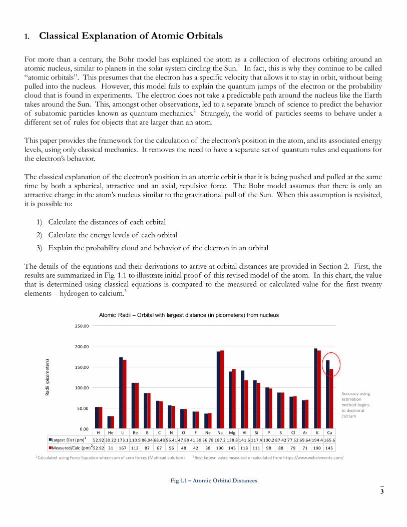
The details of the equations and their derivations to arrive at orbital distances are provided in Section 2. First, the results are summarized in Fig. 1.1 to illustrate initial proof of this revised model of the atom. In this chart, the value that is determined using classical equations is compared to the measured or calculated value for the first twenty elements – hydrogen to calcium.3
Fig 1.1 – Atomic Orbital Distances
1CalculatedusingForceEquationwheresumofzeroforces(Mathcadsolution)2Bestknownvaluemeasuredorcalculatedfromhttps://www.webelements.com/
Accuracyusingestimationmethodbeginstodeclineatcalcium
H He Li Be B C N O F Ne Na Mg Al Si P S Cl Ar K Ca
LargestDist(pm) 52.92 30.22 173.1 110.9 86.94 68.48 56.41 47.89 41.59 36.78 187.2 138.8 141.6 117.4 100.2 87.42 77.52 69.64 194.4 165.6
Measured/Calc (pm) 52.92 31 167 112 87 67 56 48 42 38 190 145 118 111 98 88 79 71 190 145
0.00
50.00
100.00
150.00
200.00
250.00
Radii(picometers)
Atomic Radii – Orbital with largest distance (in picometers) from nucleus
1
2
4
There are some variations due to two reasons: 1) the measurement of atoms from some experiments may not be precise, and 2) the angles of electrons were estimated and solved using Mathcad and the method begins to decline as the number of electrons in orbit increases or the distance to the nucleus decreases. This will be further explained in Section 2.
Fig 1.1 would not have been sufficient proof alone as it only calculated and compared the largest orbital distance for 20 elements. However, orbital distances were calculated using this classical method for all of the subshells in an atom (1s, 2s, 2p, 3s, 3p, 4s) and also for ionized elements through calcium. Since experimental evidence of orbital distances for these subshells do not exist, they can be compared to ionization energies instead. Ionization energies depend on an electron’s distance from the nucleus.
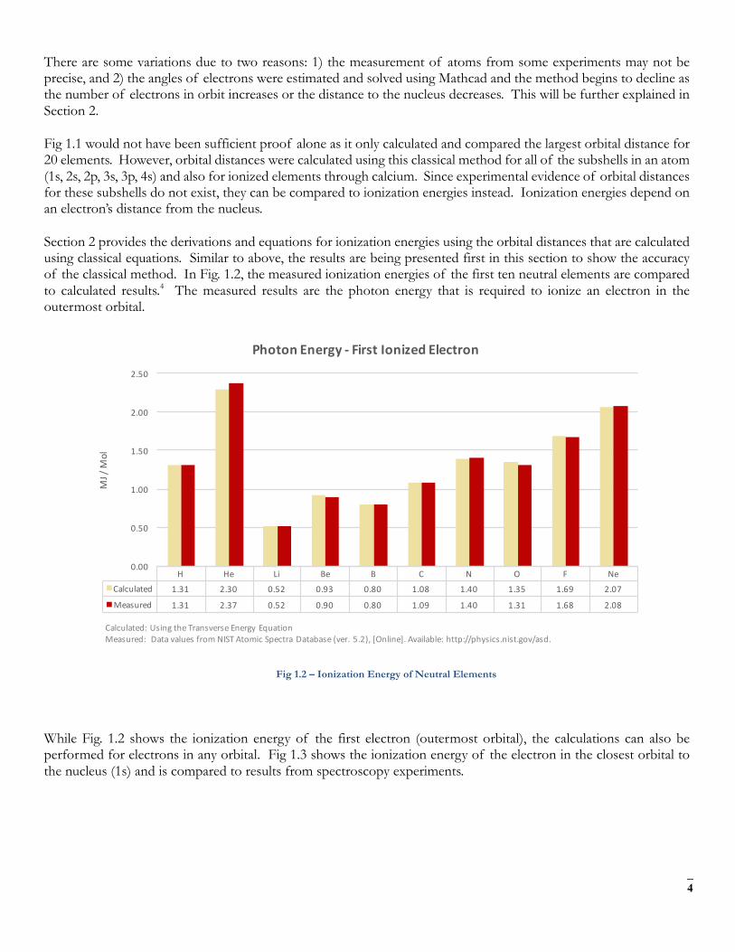
Section 2 provides the derivations and equations for ionization energies using the orbital distances that are calculated using classical equations. Similar to above, the results are being presented first in this section to show the accuracy of the classical method. In Fig. 1.2, the measured ionization energies of the first ten neutral elements are compared to calculated results.4 The measured results are the photon energy that is required to ionize an electron in the outermost orbital.
Fig 1.2 – Ionization Energy of Neutral Elements
While Fig. 1.2 shows the ionization energy of the first electron (outermost orbital), the calculations can also be performed for electrons in any orbital. Fig 1.3 shows the ionization energy of the electron in the closest orbital to the nucleus (1s) and is compared to results from spectroscopy experiments.
H He Li Be B C N O F Ne
Calculated 1.31 2.30 0.52 0.93 0.80 1.08 1.40 1.35 1.69 2.07
Measured 1.31 2.37 0.52 0.90 0.80 1.09 1.40 1.31 1.68 2.08
0.00
0.50
1.00
1.50
2.00
2.50
MJ/M
ol
PhotonEnergy- FirstIonizedElectron
Calculated:UsingtheTransverseEnergyEquationMeasured: DatavaluesfromNISTAtomicSpectraDatabase (ver. 5.2),[Online].Available: http://physics.nist.gov/asd.

5
Fig 1.3 – Ionization Energy of 1s Electron of Neutral Elements (Spectroscopy). Uses Amplitude Factor Equation.
Orbital distances were also calculated for ionized elements. Because the classical explanation of atomic orbitals is based on the interaction of each and every electron on other electrons, in addition to the nucleus, they have been grouped into atoms with a similar electron structure. For example, Fig. 1.4 lists the ionized elements with only one electron in orbit (1s1). This is the simplest arrangement as the only force on the electron is from the nucleus. For helium, it is He1+. For heavily ionized calcium, it is Ca19+. In Fig 1.4, the calculated orbital distances and ionization energies agree with the measured results.
H He Li Be B C N O F Ne Na Mg Al Si P S Cl Ar K CaCalculated 1.31 2.33 6.16 11.8 19.3 28.6 39.7 52.7 67.4 84.0 104.4126.9151.7178.7207.9239.2272.8308.6347.8389.4
Measured 1.31 2.37 6.26 11.5 19.3 28.6 39.6 52.6 67.2 84.0 104 126 151 178 208 239 273 309 347 390
0.00
50.00
100.00
150.00
200.00
250.00
300.00
350.00
400.00
450.00Mj/M
ol
PhotonEnergy- Spectroscopy1sElectron(usingAmp.FactorEquation)
Calculated:UsingtheTransverseEnergyEquation,usedradius andamplitudefactor forthespectroscopyof1selectron.Measured: Datavaluesfromhttp://cbc.arizona.edu/chemt/Flash/photoelectron.html
He1+ Li2+ Be3+ B4+ C5+ N6+ O7+ F8+ Ne9+ Na10+ Mg11+ Al12+ Si13+ P14+ S15+ Cl16+ Ar17+ K18+ Ca19+
Calculated 5.25 11.81 21.00 32.82 47.26 64.32 84.02 106.33 131.27 158.84 189.04 221.85 257.30 295.37 336.06 379.38 425.33 473.90 525.10
Measured 5.25 11.82 21.01 32.83 47.28 64.36 84.08 106.43 131.43 159.08 189.37 222.32 257.92 296.20 337.14 380.76 427.07 476.06 527.76
0.00
100.00
200.00
300.00
400.00
500.00
600.00
MJ/MOL
IONIZEDATOM ENERGY - 1S1 ELECTRON
AmplitudeRule: Z-e+1
Calculated:UsingTransverseEnergyEquation
Measured: DatavaluesfromNISTAtomicSpectraDatabase (ver. 5.2),[Online].Available: http://physics.nist.gov/asd.
6
Fig 1.4 – Ionization Energy of Ionized Elements with 1 Electron
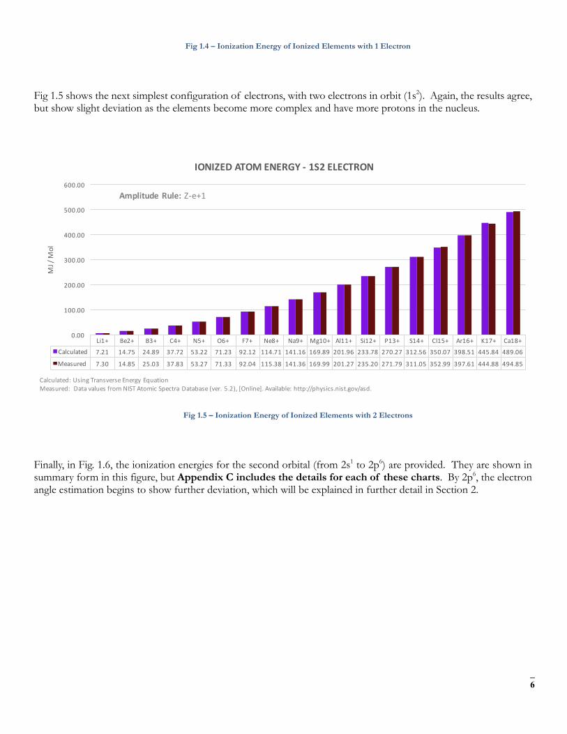
Fig 1.5 shows the next simplest configuration of electrons, with two electrons in orbit (1s2). Again, the results agree, but show slight deviation as the elements become more complex and have more protons in the nucleus.
Fig 1.5 – Ionization Energy of Ionized Elements with 2 Electrons
Finally, in Fig. 1.6, the ionization energies for the second orbital (from 2s1 to 2p6) are provided. They are shown in summary form in this figure, but Appendix C includes the details for each of these charts. By 2p6, the electron angle estimation begins to show further deviation, which will be explained in further detail in Section 2.
Li1+ Be2+ B3+ C4+ N5+ O6+ F7+ Ne8+ Na9+ Mg10+ Al11+ Si12+ P13+ S14+ Cl15+ Ar16+ K17+ Ca18+
Calculated 7.21 14.75 24.89 37.72 53.22 71.23 92.12 114.71 141.16 169.89 201.96 233.78 270.27 312.56 350.07 398.51 445.84 489.06
Measured 7.30 14.85 25.03 37.83 53.27 71.33 92.04 115.38 141.36 169.99 201.27 235.20 271.79 311.05 352.99 397.61 444.88 494.85
0.00
100.00
200.00
300.00
400.00
500.00
600.00
MJ/M
ol
IONIZEDATOMENERGY- 1S2ELECTRON
AmplitudeRule: Z-e+1
Calculated:UsingTransverseEnergyEquation
Measured: DatavaluesfromNISTAtomicSpectraDatabase (ver. 5.2),[Online].Available: http://physics.nist.gov/asd.

7
Fig 1.6 – Ionization Energy of Ionized Elements with 3 to 10 Electrons
Twenty orbital distances were calculated using classical methods and compared to measured results. More than 150 variations of neutral and ionized atoms from hydrogen to calcium were also calculated for ionization energies using the same method for orbital distances. The calculations agree with measured results. When there are deviations, there is a noticeable trend that appears as elements become more complex with increasing electrons and shorter distances to the nucleus. With greater accuracy in computer modeling of electron angles, it is expected that these deviations should disappear.
In addition to orbital calculations and ionization energies, an explanation is provided for orbital shapes in Section 3. Orbital shapes are attributed to a tetrahedral nucleus structure and an arrangement of protons that cause a greater repulsion factor when protons and spins are aligned. This same tetrahedral structure is then expanded upon in Section 4 to explain the sequence of the Periodic Table of Elements.
The equations used to derive an electron’s distance and energy use a common set of constants that were found to calculate a particle’s rest mass like the electron, unite the major forces, derive 19 fundamental physical constants and derive 6 common energy and force equations in physics. They are found in papers: Particle Energy and Interaction5, Forces6, Fundamental Physical Constants7 and Key Physics Equations and Experiments8. These constants and their notation are found below in Section 1.1.
0.0020.0040.0060.0080.00100.00120.00
Be1+
N4+
Ne7+
Al10
+ S13+
K1
6+
2S1
020406080
100120
B1+
N3+
F5+
Na7+
Al9+
P11+
Cl13
+ K1
5+
2S2
0
20
40
60
80
100
N1+
F3+
Na5+
Al7+
P9+
Cl11
+ K1
3+
2P2
0.0020.0040.0060.0080.00100.00
O1+
Ne3+
Mg5+
Si7+
S9+
Ar11
+ Ca13
+
2P3
0
20
40
60
80
F1+
Na3+
Al5+
P7+
Cl9+
K11+
2P4
0.00
20.00
40.00
60.00
80.00
Ne1+
Mg3+
Si5+
S7+
Ar9+
Ca11
+
2P5
0.00
20.00
40.00
60.00
80.00
Na1+
Al3+
P5+
Cl7+
K9+
2P6
0.0020.0040.0060.0080.00100.00
C1+
O3+
Ne5+
Mg7+
Si9+
S11+
Ar13
+ Ca15
+
2P1
8
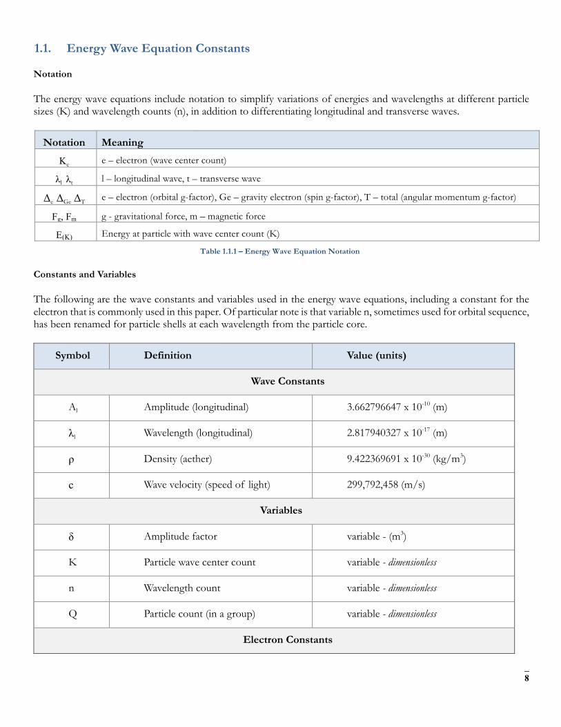
1.1. Energy Wave Equation Constants
Notation
The energy wave equations include notation to simplify variations of energies and wavelengths at different particle sizes (K) and wavelength counts (n), in addition to differentiating longitudinal and transverse waves.
Notation Meaning
Ke e – electron (wave center count)
λl λt l – longitudinal wave, t – transverse wave
Δe ΔGe ΔT e – electron (orbital g-factor), Ge – gravity electron (spin g-factor), T – total (angular momentum g-factor)
Fg, Fm g - gravitational force, m – magnetic force
E(K) Energy at particle with wave center count (K) Table 1.1.1 – Energy Wave Equation Notation
Constants and Variables
The following are the wave constants and variables used in the energy wave equations, including a constant for the electron that is commonly used in this paper. Of particular note is that variable n, sometimes used for orbital sequence, has been renamed for particle shells at each wavelength from the particle core.
Symbol Definition Value (units)
Wave Constants
Al Amplitude (longitudinal) 3.662796647 x 10⁻¹⁰ (m)
λl Wavelength (longitudinal) 2.817940327 x 10⁻¹⁷ (m)
ρ Density (aether) 9.422369691 x 10⁻³⁰ (kg/m3)
c Wave velocity (speed of light) 299,792,458 (m/s)
Variables
δ Amplitude factor variable - (m3)
K Particle wave center count variable - dimensionless
n Wavelength count variable - dimensionless
Q Particle count (in a group) variable - dimensionless
Electron Constants
9
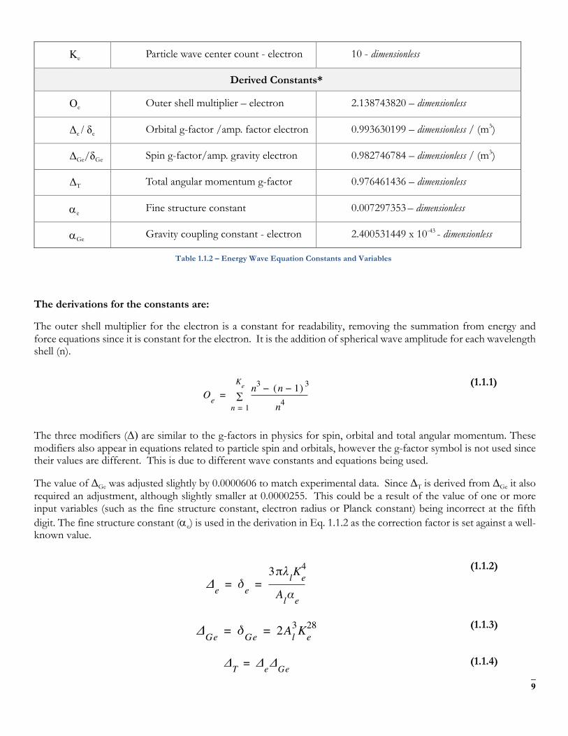
Ke Particle wave center count - electron 10 - dimensionless
Derived Constants*
Oe Outer shell multiplier – electron 2.138743820 – dimensionless
Δe / δe Orbital g-factor /amp. factor electron 0.993630199 – dimensionless / (m3)
ΔGe/δGe Spin g-factor/amp. gravity electron 0.982746784 – dimensionless / (m3)
ΔT Total angular momentum g-factor 0.976461436 – dimensionless
ae Fine structure constant 0.007297353 – dimensionless
aGe Gravity coupling constant - electron 2.400531449 x 10-43 - dimensionless
Table 1.1.2 – Energy Wave Equation Constants and Variables
The derivations for the constants are:
The outer shell multiplier for the electron is a constant for readability, removing the summation from energy and force equations since it is constant for the electron. It is the addition of spherical wave amplitude for each wavelength shell (n).
(1.1.1)
The three modifiers (Δ) are similar to the g-factors in physics for spin, orbital and total angular momentum. These modifiers also appear in equations related to particle spin and orbitals, however the g-factor symbol is not used since their values are different. This is due to different wave constants and equations being used.
The value of ΔGe was adjusted slightly by 0.0000606 to match experimental data. Since ΔT is derived from ΔGe it also required an adjustment, although slightly smaller at 0.0000255. This could be a result of the value of one or more input variables (such as the fine structure constant, electron radius or Planck constant) being incorrect at the fifth digit. The fine structure constant (ae) is used in the derivation in Eq. 1.1.2 as the correction factor is set against a well-known value.
(1.1.2)
(1.1.3)
(1.1.4)
Oen3 n 1−( ) 3−
n4n 1=
Ke∑=
Δe δe3πλlKe
4
Alαe= =
ΔGe δGe 2Al3Ke
28= =
ΔT ΔeΔGe=
10
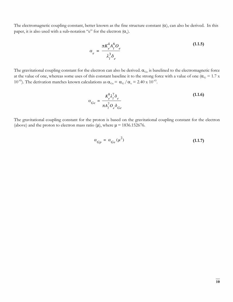
The electromagnetic coupling constant, better known as the fine structure constant (a), can also be derived. In this paper, it is also used with a sub-notation “e” for the electron (ae).
(1.1.5)
The gravitational coupling constant for the electron can also be derived. aGe is baselined to the electromagnetic force at the value of one, whereas some uses of this constant baseline it to the strong force with a value of one (aG = 1.7 x 10-45). The derivation matches known calculations as aGe = aG / ae = 2.40 x 10-43.
(1.1.6)
The gravitational coupling constant for the proton is based on the gravitational coupling constant for the electron (above) and the proton to electron mass ratio (µ), where µ = 1836.152676.
(1.1.7)
αeπKe
4Al6Oe
λl3δe
=
αGeKe8λl7δe
πAl7OeδGe
=
αGp αGe µ2( )=
11
2. Orbital Distances and Energies
This section provides the derivation of classical equations to calculate the orbital distances and ionization energies of elements from hydrogen to calcium that were graphed and compared against measured results in Section 1.
2.1. Classical Explanation of Orbital Distances
In Section 1, an introductory explanation of the electron’s orbital distance was described as a nucleus that has both a spherical, attractive force and an axial, repulsive force. The electron is being both pushed and pulled by a proton and the orbital is the point where the sum of the forces on the electron is zero.
This explanation requires a model of the proton that is also found in the Forces paper and is consistent with a pentaquark model of the proton, which includes four quarks and one anti-quark. An explanation for why three quarks are often found in proton collision experiments is provided in Forces. Here, the forces are described.
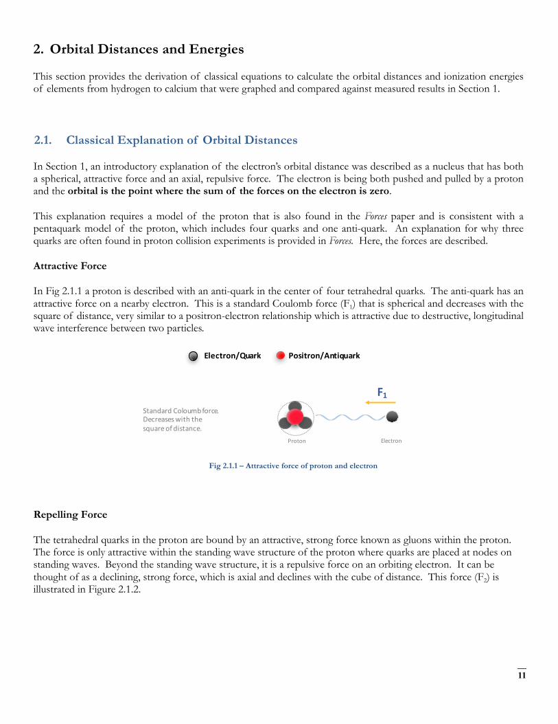
Attractive Force
In Fig 2.1.1 a proton is described with an anti-quark in the center of four tetrahedral quarks. The anti-quark has an attractive force on a nearby electron. This is a standard Coulomb force (F1) that is spherical and decreases with the square of distance, very similar to a positron-electron relationship which is attractive due to destructive, longitudinal wave interference between two particles.
Fig 2.1.1 – Attractive force of proton and electron
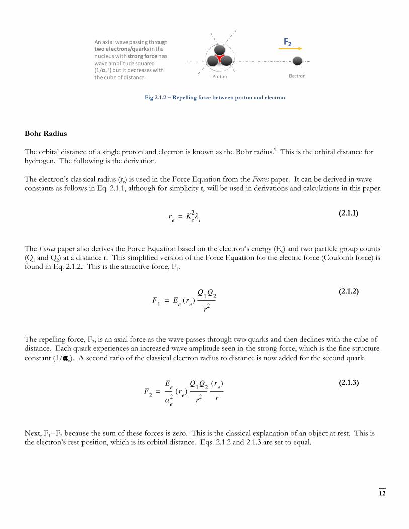
Repelling Force
The tetrahedral quarks in the proton are bound by an attractive, strong force known as gluons within the proton. The force is only attractive within the standing wave structure of the proton where quarks are placed at nodes on standing waves. Beyond the standing wave structure, it is a repulsive force on an orbiting electron. It can be thought of as a declining, strong force, which is axial and declines with the cube of distance. This force (F2) is illustrated in Figure 2.1.2.
Electron/Quark Positron/Antiquark
Proton Electron
F1StandardColoumbforce.Decreaseswiththesquareofdistance.
12
Fig 2.1.2 – Repelling force between proton and electron
Bohr Radius
The orbital distance of a single proton and electron is known as the Bohr radius.9 This is the orbital distance for hydrogen. The following is the derivation.
The electron’s classical radius (re) is used in the Force Equation from the Forces paper. It can be derived in wave constants as follows in Eq. 2.1.1, although for simplicity re will be used in derivations and calculations in this paper.
(2.1.1)
The Forces paper also derives the Force Equation based on the electron’s energy (Ee) and two particle group counts (Q1 and Q2) at a distance r. This simplified version of the Force Equation for the electric force (Coulomb force) is found in Eq. 2.1.2. This is the attractive force, F1.
(2.1.2)
The repelling force, F2, is an axial force as the wave passes through two quarks and then declines with the cube of distance. Each quark experiences an increased wave amplitude seen in the strong force, which is the fine structure constant (1/⍺ e). A second ratio of the classical electron radius to distance is now added for the second quark.
(2.1.3)
Next, F1=F2 because the sum of these forces is zero. This is the classical explanation of an object at rest. This is the electron’s rest position, which is its orbital distance. Eqs. 2.1.2 and 2.1.3 are set to equal.
Proton Electron
Anaxialwavepassingthroughtwoelectrons/quarks inthenucleuswithstrongforcehaswaveamplitudesquared(1/⍺e
2)butitdecreaseswiththecubeofdistance.
F2
re Ke2λl=
F1 Ee re( )Q1Q2
r2=
F2Ee
αe2re( )
Q1Q2
r2
re( )
r=
13
(2.1.4)
After solving for r in Eq. 2.1.4, it is found to be the Bohr radius (5.2918 x 10⁻¹¹ meters).10
(2.1.5)
The Bohr radius is the simplest orbital distance to calculate as it has two forces to consider due to two particles: one electron and one proton. At the end of this section, a methodology is created for considering the force of multiple protons and electrons in an atom to calculate various orbital distances. First, the quantum leap of the orbital must be explained beyond the 1s orbital.
2.2. Classical Explanation of Orbital Quantum Leaps
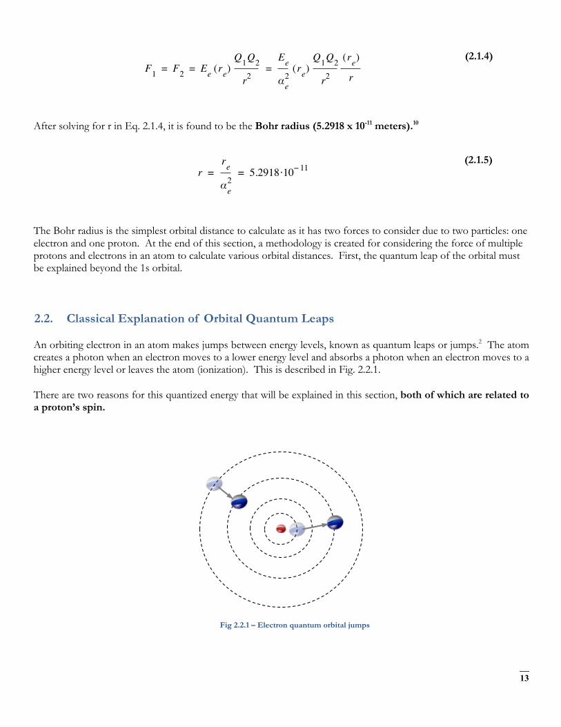
An orbiting electron in an atom makes jumps between energy levels, known as quantum leaps or jumps.2 The atom creates a photon when an electron moves to a lower energy level and absorbs a photon when an electron moves to a higher energy level or leaves the atom (ionization). This is described in Fig. 2.2.1.
There are two reasons for this quantized energy that will be explained in this section, both of which are related to a proton’s spin.
Fig 2.2.1 – Electron quantum orbital jumps
F1 F2 Ee re( )Q1Q2
r2
Ee
αe2re( )
Q1Q2
r2
re( )
r= = =
rre
αe2
5.2918 10 11−·= =
14
Protons have a similar spin as electrons. In the revised pentaquark model of the proton, there are four tetrahedral quarks and an anti-quark in the middle. The tetrahedral quarks cancel spin (+ ½, + ½, - ½, - ½), leaving the anti-quark/positron in the center that is responsible for the spin. It has value + ½ or - ½.
The anti-quark/positron reflects longitudinal waves that is responsible for the electric force (Coulomb force), but its spin also creates a second, transverse wave as illustrated in Fig. 2.2.2 in red.
Fig 2.2.2 – Proton’s spin (anti-quark/positron spin in the center)
There are two directions for spin, otherwise referred to as spin-up or spin-down in physics. Since quantum jumps are related to the arrangement of protons in the nucleus, which is affected by their tetrahedral structure, the following icons are used in this theory:
Fig 2.2.3 – Proton’s icons for spin-up and spin-down showing tetrahedral quark alignment
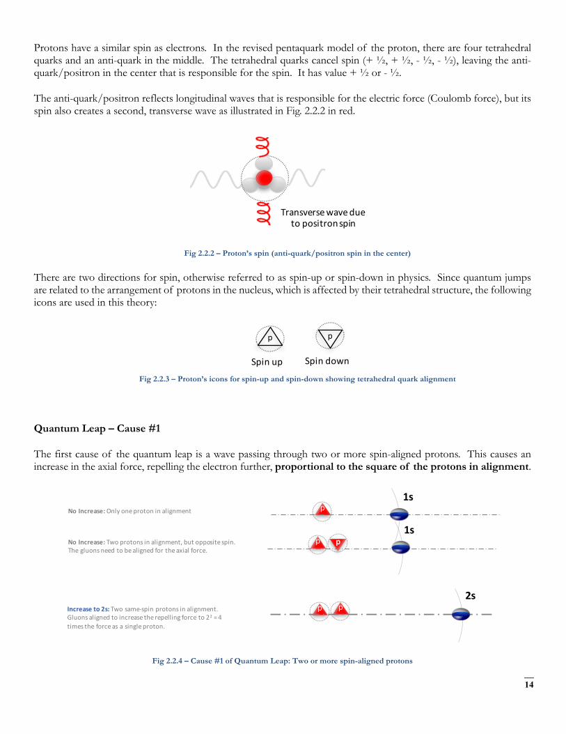
Quantum Leap – Cause #1
The first cause of the quantum leap is a wave passing through two or more spin-aligned protons. This causes an increase in the axial force, repelling the electron further, proportional to the square of the protons in alignment.
Fig 2.2.4 – Cause #1 of Quantum Leap: Two or more spin-aligned protons
Transversewaveduetopositronspin
Spinup Spindown
p p
p p2s
p p1s
p1s
NoIncrease:Onlyoneprotoninalignment
NoIncrease:Twoprotonsinalignment,butoppositespin.Thegluonsneedtobealignedfortheaxialforce.
Increaseto2s:Twosame-spinprotonsinalignment.Gluonsalignedtoincreasetherepellingforceto22=4timestheforceasasingleproton.
15
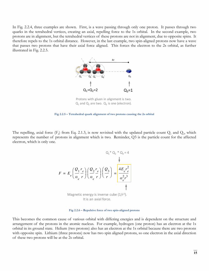
In Fig. 2.2.4, three examples are shown. First, is a wave passing through only one proton. It passes through two quarks in the tetrahedral vertices, creating an axial, repelling force to the 1s orbital. In the second example, two protons are in alignment, but the tetrahedral vertices of these protons are not in alignment, due to opposite spins. It therefore repels to the 1s orbital distance. However, in the last example, two spin-aligned protons now have a wave that passes two protons that have their axial force aligned. This forces the electron to the 2s orbital, as further illustrated in Fig. 2.2.5.
Fig 2.2.5 – Tetrahedral quark alignment of two protons causing the 2s orbital
The repelling, axial force (F2) from Eq. 2.1.3, is now revisited with the updated particle count Q1 and Q2, which represents the number of protons in alignment which is two. Reminder, Q3 is the particle count for the affected electron, which is only one.
Fig 2.2.6 – Repulsive force of two spin-aligned protons
This becomes the common cause of various orbital with differing energies and is dependent on the structure and arrangement of the protons in the atomic nucleus. For example, hydrogen (one proton) has an electron at the 1s orbital in its ground state. Helium (two protons) also has an electron at the 1s orbital because there are two protons with opposite spin. Lithium (three protons) now has two spin aligned protons, so one electron in the axial direction of these two protons will be at the 2s orbital.
Q1 Q3
p
Q2
4r
Q1
p
Q2
Q1=Q2=2 Q3=1
Protonswithgluoninalignmentistwo.Q1 andQ2 aretwo.Q3 isone(electron).
Magneticenergyisinversecube(1/r3).Itisanaxialforce.
F EeQ1αe
rer⎝ ⎠
⎜ ⎟⎛ ⎞ Q2
αe
rer⎝ ⎠
⎜ ⎟⎛ ⎞ Q3
r⎝ ⎠⎜ ⎟⎛ ⎞ 4Eere
2
αe2r3
= =
Q1*Q2 *Q3=4
16
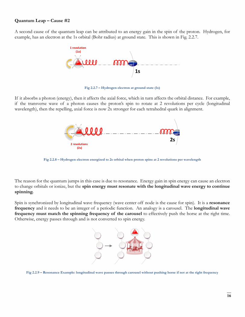
Quantum Leap – Cause #2
A second cause of the quantum leap can be attributed to an energy gain in the spin of the proton. Hydrogen, for example, has an electron at the 1s orbital (Bohr radius) at ground state. This is shown in Fig. 2.2.7.
Fig 2.2.7 – Hydrogen electron at ground state (1s)
If it absorbs a photon (energy), then it affects the axial force, which in turn affects the orbital distance. For example, if the transverse wave of a photon causes the proton’s spin to rotate at 2 revolutions per cycle (longitudinal wavelength), then the repelling, axial force is now 2x stronger for each tetrahedral quark in alignment.
Fig 2.2.8 – Hydrogen electron energized to 2s orbital when proton spins at 2 revolutions per wavelength
The reason for the quantum jumps in this case is due to resonance. Energy gain in spin energy can cause an electron to change orbitals or ionize, but the spin energy must resonate with the longitudinal wave energy to continue spinning.
Spin is synchronized by longitudinal wave frequency (wave center off node is the cause for spin). It is a resonance frequency and it needs to be an integer of a periodic function. An analogy is a carousel. The longitudinal wave frequency must match the spinning frequency of the carousel to effectively push the horse at the right time. Otherwise, energy passes through and is not converted to spin energy.
Fig 2.2.9 – Resonance Example: longitudinal wave passes through carousel without pushing horse if not at the right frequency
p

17
Longitudinal wave amplitude can increase and cause faster spin, but it can only be 1x, 2x, 3x, etc in integers, because the rotation must match the periodic frequency of longitudinal waves. E.g. 2x wave amplitude is 2x rotational spin; but 1.5x wave amplitude is still only 1x rotational spin. Thus, the electron would fall back to the 1s orbital, vibrating into position and creating a new photon with this transverse energy as it settles back to 1s.
Fig 2.2.9 – Resonance Example: longitudinal wave pushes horse, transferring longitudinal energy to transverse energy
This explanation of spin and resonance frequency can now be modeled mathematically. First, the standard force equation for the axial, repelling force is shown again for a proton resonating with longitudinal waves.
Fig 2.2.10 – Repelling force equation for proton with standard (1x) spin
This is compared to a proton that absorbs a photon, which is transverse energy, causing the spin of the proton to change. If the energy is sufficient to reach two revolutions per longitudinal wavelength (2x), it can now continue to spin at that frequency. The equation is shown in Fig. 2.2.11. The fine structure (ae) is the wave amplitude change between quarks for the strong force, which is now modified to be 2x greater for each quark in axial alignment. Note that it is the inverse of the fine structure constant that is the increase in wave amplitude or (ae/2).
p
Q1 Q3
p
Q2
r
Singleprotonalignment - 1xspin
F EeQ1αe
rer⎝ ⎠
⎜ ⎟⎛ ⎞ Q2
αe
rer⎝ ⎠
⎜ ⎟⎛ ⎞ Q3
r⎝ ⎠⎜ ⎟⎛ ⎞ Eere
2
αe2r3
= =
*Usingshorthand notation forforceequation
Q1=Q2=Q3=1
18
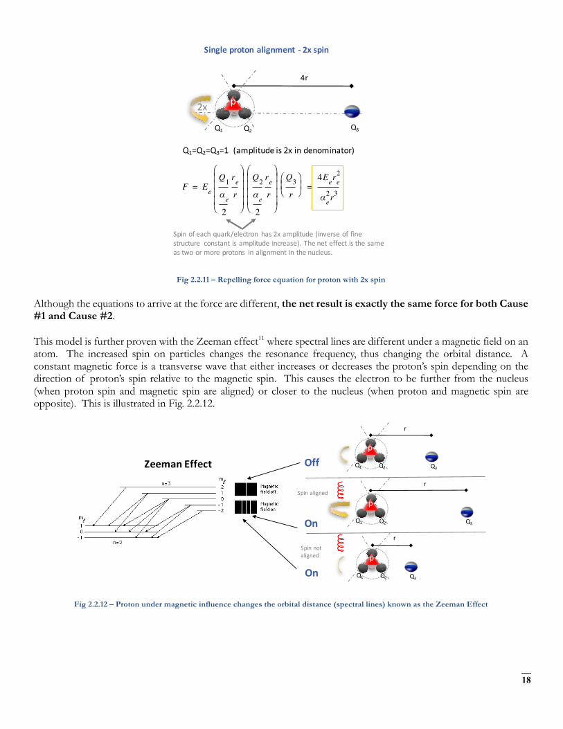
Fig 2.2.11 – Repelling force equation for proton with 2x spin
Although the equations to arrive at the force are different, the net result is exactly the same force for both Cause #1 and Cause #2.
This model is further proven with the Zeeman effect11 where spectral lines are different under a magnetic field on an atom. The increased spin on particles changes the resonance frequency, thus changing the orbital distance. A constant magnetic force is a transverse wave that either increases or decreases the proton’s spin depending on the direction of proton’s spin relative to the magnetic spin. This causes the electron to be further from the nucleus (when proton spin and magnetic spin are aligned) or closer to the nucleus (when proton and magnetic spin are opposite). This is illustrated in Fig. 2.2.12.
Fig 2.2.12 – Proton under magnetic influence changes the orbital distance (spectral lines) known as the Zeeman Effect
Q1 Q3
p
Q2
4r
2x
Singleprotonalignment - 2xspin
F EeQ1αe2
rer
⎝ ⎠⎜ ⎟⎜ ⎟⎜ ⎟⎜ ⎟⎛ ⎞
Q2αe2
rer
⎝ ⎠⎜ ⎟⎜ ⎟⎜ ⎟⎜ ⎟⎛ ⎞
Q3r⎝ ⎠
⎜ ⎟⎛ ⎞ 4Eere
2
αe2r3
= =
Q1=Q2=Q3=1(amplitudeis2xindenominator)
Spinofeachquark/electron has2xamplitude(inverseoffinestructure constantisamplitudeincrease).Theneteffectisthesameastwoormoreprotons inalignmentinthenucleus.
ZeemanEffect Q1 Q3
p
Q2
r
Off
Q1 Q3
p
Q2
r
On
Q1 Q3
p
Q2On
r
Spinaligned
Spinnotaligned
19
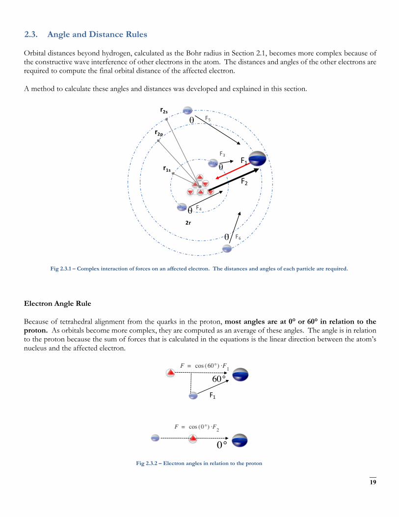
2.3. Angle and Distance Rules
Orbital distances beyond hydrogen, calculated as the Bohr radius in Section 2.1, becomes more complex because of the constructive wave interference of other electrons in the atom. The distances and angles of the other electrons are required to compute the final orbital distance of the affected electron.
A method to calculate these angles and distances was developed and explained in this section.
Fig 2.3.1 – Complex interaction of forces on an affected electron. The distances and angles of each particle are required.
Electron Angle Rule
Because of tetrahedral alignment from the quarks in the proton, most angles are at 0° or 60° in relation to the proton. As orbitals become more complex, they are computed as an average of these angles. The angle is in relation to the proton because the sum of forces that is calculated in the equations is the linear direction between the atom’s nucleus and the affected electron.
Fig 2.3.2 – Electron angles in relation to the proton
r1s
2r
F1F3
F2
r2p
r2s
F4
F5
F6
θ
θ
θ
θ
F1
60°
0°
20
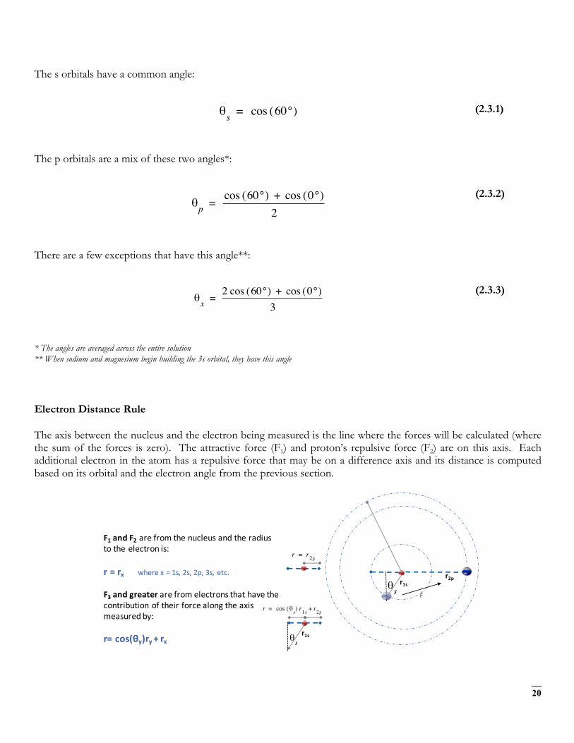
The s orbitals have a common angle:
(2.3.1)
The p orbitals are a mix of these two angles*:
(2.3.2)
There are a few exceptions that have this angle**:
(2.3.3)
* The angles are averaged across the entire solution ** When sodium and magnesium begin building the 3s orbital, they have this angle
Electron Distance Rule
The axis between the nucleus and the electron being measured is the line where the forces will be calculated (where the sum of the forces is zero). The attractive force (F1) and proton’s repulsive force (F2) are on this axis. Each additional electron in the atom has a repulsive force that may be on a difference axis and its distance is computed based on its orbital and the electron angle from the previous section.
θs 60°( )cos=
θp60°( )cos 0°( )cos+
2=
θx2 60°( )cos 0°( )cos+
3=
F1 andF2 arefromthenucleusandtheradiustotheelectronis:
r=rx wherex=1s,2s,2p,3s, etc.
F3 andgreaterarefromelectronsthathavethecontributionoftheirforcealongtheaxismeasuredby:
r=cos(θy)ry +rx
r1sF
r2pθs
r1sθs
r r2p=
r θs( ) r1scos r2p+=
21
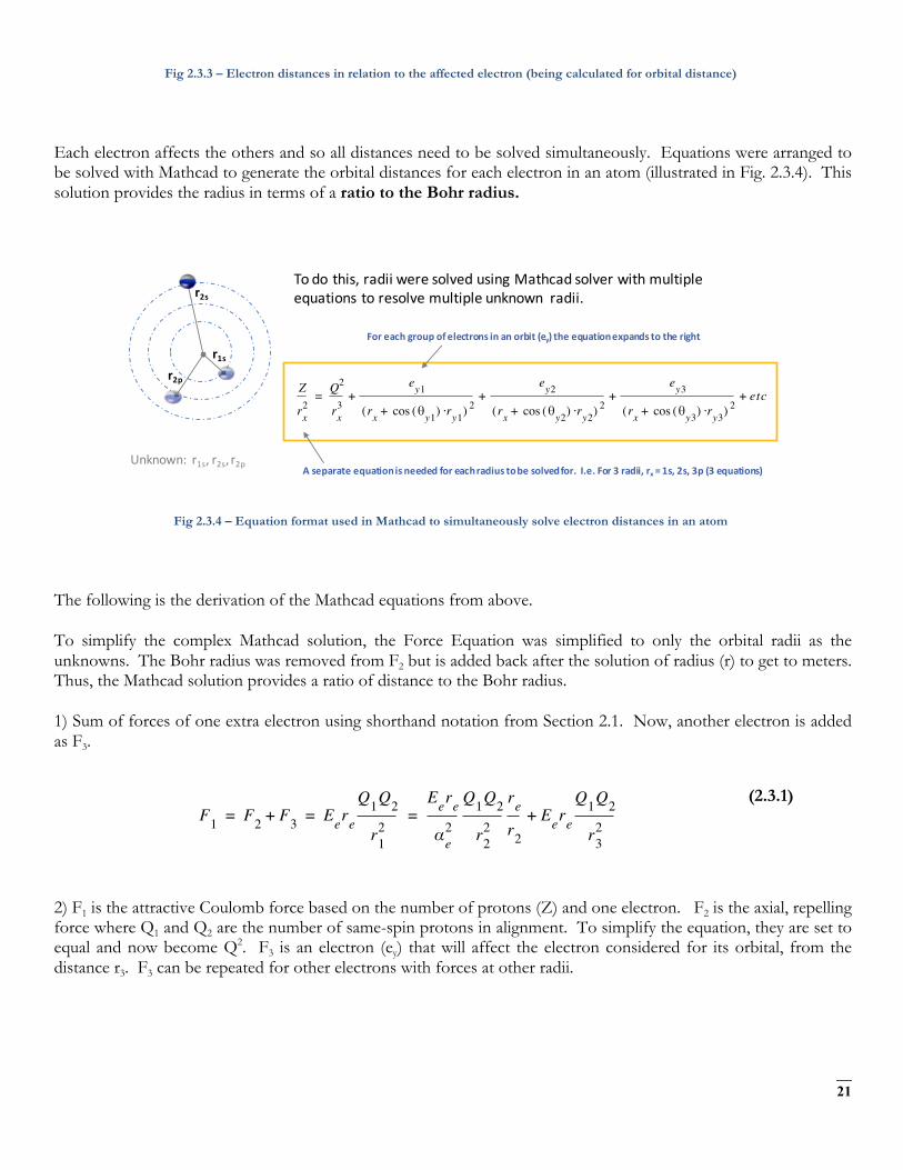
Fig 2.3.3 – Electron distances in relation to the affected electron (being calculated for orbital distance)
Each electron affects the others and so all distances need to be solved simultaneously. Equations were arranged to be solved with Mathcad to generate the orbital distances for each electron in an atom (illustrated in Fig. 2.3.4). This solution provides the radius in terms of a ratio to the Bohr radius.
Fig 2.3.4 – Equation format used in Mathcad to simultaneously solve electron distances in an atom
The following is the derivation of the Mathcad equations from above.
To simplify the complex Mathcad solution, the Force Equation was simplified to only the orbital radii as the unknowns. The Bohr radius was removed from F2 but is added back after the solution of radius (r) to get to meters. Thus, the Mathcad solution provides a ratio of distance to the Bohr radius.
1) Sum of forces of one extra electron using shorthand notation from Section 2.1. Now, another electron is added as F3.
(2.3.1)
2) F1 is the attractive Coulomb force based on the number of protons (Z) and one electron. F2 is the axial, repelling force where Q1 and Q2 are the number of same-spin protons in alignment. To simplify the equation, they are set to equal and now become Q2. F3 is an electron (ey) that will affect the electron considered for its orbital, from the distance r3. F3 can be repeated for other electrons with forces at other radii.
r2p
r2s
r1s
Unknown: r1s,r2s,r2p
Todothis,radiiweresolvedusingMathcadsolverwithmultipleequationstoresolvemultipleunknown radii.
Z
rx2
Q2
rx3
ey1
rx θy1( )cos ry1·+( ) 2
ey2
rx θy2( )cos ry2·+( ) 2
ey3
rx θy3( )cos ry3·+( ) 2etc+ + + +=
Aseparateequationisneededforeachradiustobesolvedfor.I.e.For3radii,rx =1s,2s,3p(3equations)
Foreachgroupofelectronsinanorbit(ey)theequationexpandstotheright
F1 F2 F3+ EereQ1Q2
r12
Eere
αe2
Q1Q2
r22
rer2
EereQ1Q2
r32
+= = =
22
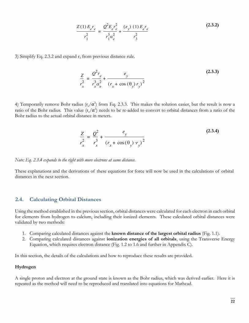
(2.3.2)
3) Simplify Eq. 2.3.2 and expand r3 from previous distance rule.
(2.3.3)
4) Temporarily remove Bohr radius (re/⍺2) from Eq. 2.3.3. This makes the solution easier, but the result is now a ratio of the Bohr radius. This value (re/⍺2) needs to be re-added to convert to orbital distances from a ratio of the Bohr radius to the actual orbital distance in meters.
(2.3.4)
Note: Eq. 2.3.4 expands to the right with more electrons at same distance.
These explanations and the derivations of these equations for force will now be used in the calculations of orbital distances in the next section.
2.4. Calculating Orbital Distances
Using the method established in the previous section, orbital distances were calculated for each electron in each orbital for elements from hydrogen to calcium, including their ionized elements. These calculated orbital distances were validated by two methods:
1. Comparing calculated distances against the known distance of the largest orbital radius (Fig. 1.1). 2. Comparing calculated distances against ionization energies of all orbitals, using the Transverse Energy
Equation, which requires electron distance (Fig. 1.2 to 1.6 and further in Appendix C).
In this section, the details of the calculations and how to reproduce these results are provided.
Hydrogen
A single proton and electron at the ground state is known as the Bohr radius, which was derived earlier. Here it is repeated as the method will need to be reproduced and translated into equations for Mathcad.
Z 1( ) Eere
r12
Q2Eere2
r13αe2
ey( ) 1( ) Eere
r32
+=
Z
rx2
Q2re
rx3αe2
ey
rx θy( ) rycos+( ) 2+=
Z
rx2
Q2
rx3
ey
rx θy( )cos ry·+( ) 2+=
23
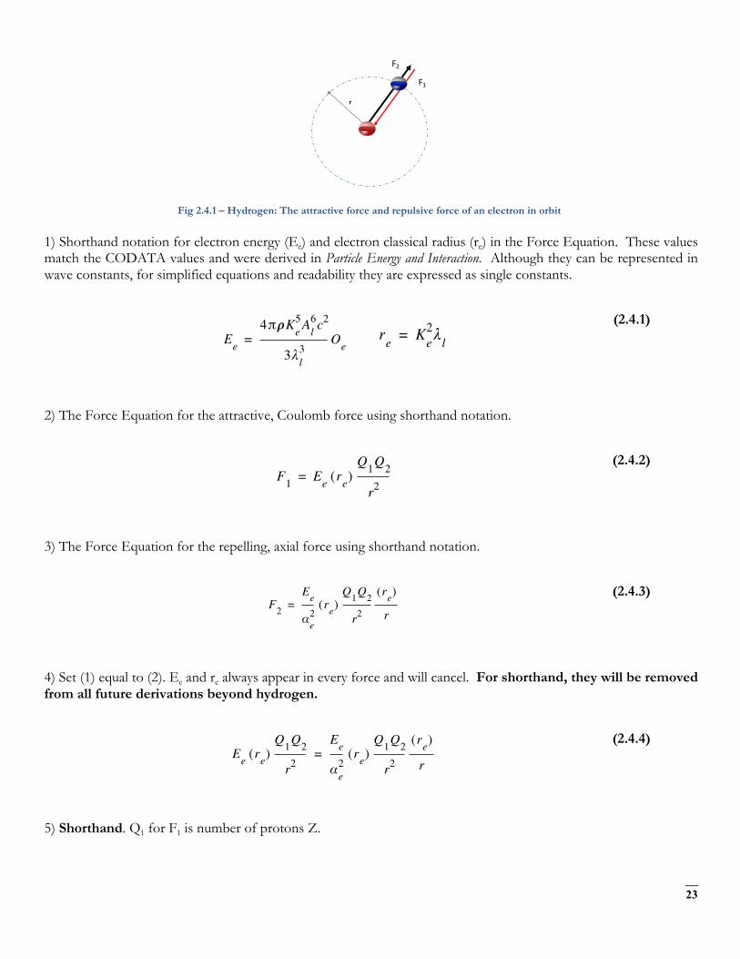
Fig 2.4.1 – Hydrogen: The attractive force and repulsive force of an electron in orbit
1) Shorthand notation for electron energy (Ee) and electron classical radius (re) in the Force Equation. These values match the CODATA values and were derived in Particle Energy and Interaction. Although they can be represented in wave constants, for simplified equations and readability they are expressed as single constants.
(2.4.1)
2) The Force Equation for the attractive, Coulomb force using shorthand notation.
(2.4.2)
3) The Force Equation for the repelling, axial force using shorthand notation.
(2.4.3)
4) Set (1) equal to (2). Ee and re always appear in every force and will cancel. For shorthand, they will be removed from all future derivations beyond hydrogen.
(2.4.4)
5) Shorthand. Q1 for F1 is number of protons Z.
r
F1
F2
re Ke2λl=Ee
4π!Ke5Al6c2
3λl3
Oe=
F1 Ee re( )Q1Q2
r2=
F2Ee
αe2re( )
Q1Q2
r2
re( )
r=
Ee re( )Q1Q2
r2
Ee
αe2re( )
Q1Q2
r2
re( )
r=
24
(2.4.5)
6) Solve for r and the solution is 5.2918 x 10⁻¹¹ m (52.9 pm). This is the exact value of the Bohr radius.
(2.4.6)
Helium
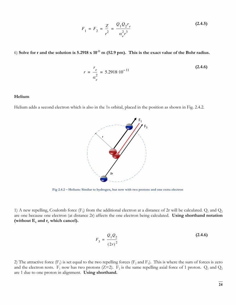
Helium adds a second electron which is also in the 1s orbital, placed in the position as shown in Fig. 2.4.2.
Fig 2.4.2 – Helium: Similar to hydrogen, but now with two protons and one extra electron
1) A new repelling, Coulomb force (F3) from the additional electron at a distance of 2r will be calculated. Q1 and Q2 are one because one electron (at distance 2r) affects the one electron being calculated. Using shorthand notation (without Ee and re which cancel).
(2.4.6)
2) The attractive force (F1) is set equal to the two repelling forces (F2 and F3). This is where the sum of forces is zero and the electron rests. F1 now has two protons (Z=2). F2 is the same repelling axial force of 1 proton. Q1 and Q2 are 1 due to one proton in alignment. Using shorthand.
F1 F2Z
r2
Q1Q2re
αe2r3
= = =
rre
αe2
5.2918 10 11−·= =
r
2r
F1F3
F3Q1Q2
2r( ) 2=
25
(2.4.7)
3) Solve for r in Eq. 2.4.7. Helium 1s orbital distance is calculated to be 30.2 pm. This is compared with an estimated radius of 31 pm from experiments.12
(2.4.8)
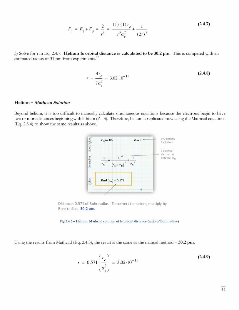
Helium – Mathcad Solution
Beyond helium, it is too difficult to manually calculate simultaneous equations because the electrons begin to have two or more distances beginning with lithium (Z=3). Therefore, helium is replicated now using the Mathcad equations (Eq. 2.3.4) to show the same results as above.
Fig 2.4.3 – Helium: Mathcad solution of 1s orbital distance (ratio of Bohr radius)
Using the results from Mathcad (Eq. 2.4.3), the result is the same as the manual method – 30.2 pm.
(2.4.9)
F1 F2 F3+ 2
r2
1( ) 1( ) re
r3αe2
1
2r( ) 2+= = =
r4re
7αe2
3.02 10 11−·= =
Distance:0.571ofBohrradius.Toconverttometers,multiplybyBohrradius.30.2pm.
Z=2protonsforhelium
1externalelectron atdistance2r1s
r 0.571re
αe2
⎝ ⎠⎜ ⎟⎜ ⎟⎛ ⎞
3.02 10 11−·= =

26
Lithium – Mathcad Solution
The equations become more complex beginning with lithium (Z=3) because it begins a new orbital (2s). Therefore, a second equation is required to simultaneously solve the 1s and 2s orbital distances. Each new orbital requires a new equation and appends more repulsive electrons to each equation being solved. These explanations are annotated along with the Mathcad solution in Fig. 2.4.4.
Fig 2.4.4 – Lithium: Mathcad solution of 1s and 2s orbital distances (ratio of Bohr radius)
The solution provides the 1s and 2s orbital distances as a ratio of the Bohr radius as 0.397 and 3.272 respectively. In picometers, these distances are 21 pm and 173 pm. The largest distance (2s) was then plotted in the graph in Fig. 1.1.
(2.4.10)
(2.4.11)
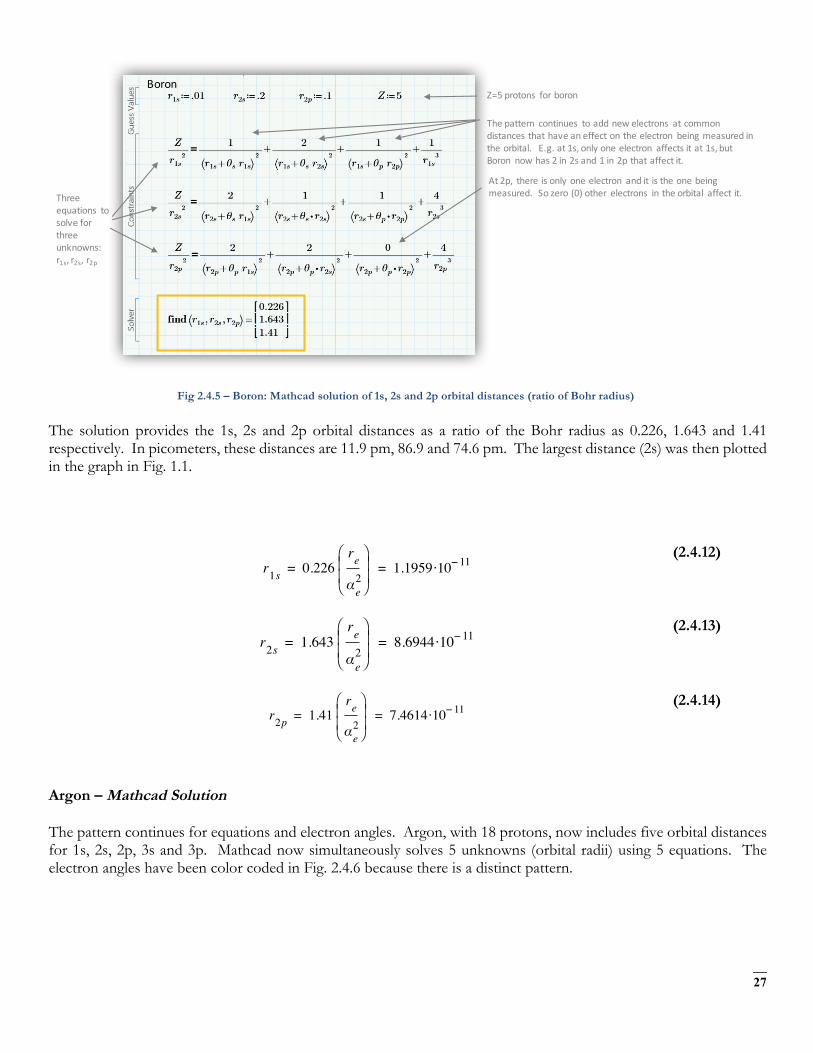
Boron – Mathcad Solution
Boron is the next example, as it now begins the transition to the 2p orbital. Since this is a third distance to calculate, a third equation is added and each equation expands to the right to include the effect of the electron at the 2p orbital distance. Also, this is the first time that the electron angles for the p orbital (θp) needs to be considered. Again, annotations in Fig. 2.4.5 explain the changes at Boron to construct the equations that yield the orbital distances.
LithiumZ=3protonsforlithium
Q=2(4afterbeingsquared)which istherepellingforcetocausetheelectron tobeatthe2nd orbital
1electron atthe1sorbital and1electron at2sorbitalthathaveaforceonanelectron inthe1sorbital (theother 1selectron)
Otherthanthe2selectron beingmeasured,therearenoother 2selectrons. Onlythe2electrons in1shaveanaffectonit.
Lithium isnowtetrahedral. Hasathetavaluethataffectsthedistancer– fromdistancerule.
r1s 0.397re
αe2
⎝ ⎠⎜ ⎟⎜ ⎟⎛ ⎞
2.10 10 11−·= =
r2s 3.272re
αe2
⎝ ⎠⎜ ⎟⎜ ⎟⎛ ⎞
1.7315 10 10−·= =
27
Fig 2.4.5 – Boron: Mathcad solution of 1s, 2s and 2p orbital distances (ratio of Bohr radius)
The solution provides the 1s, 2s and 2p orbital distances as a ratio of the Bohr radius as 0.226, 1.643 and 1.41 respectively. In picometers, these distances are 11.9 pm, 86.9 and 74.6 pm. The largest distance (2s) was then plotted in the graph in Fig. 1.1.
(2.4.12)
(2.4.13)
(2.4.14)
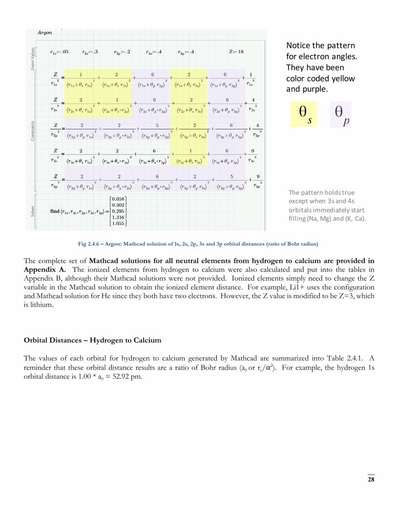
Argon – Mathcad Solution
The pattern continues for equations and electron angles. Argon, with 18 protons, now includes five orbital distances for 1s, 2s, 2p, 3s and 3p. Mathcad now simultaneously solves 5 unknowns (orbital radii) using 5 equations. The electron angles have been color coded in Fig. 2.4.6 because there is a distinct pattern.
BoronZ=5protons forboron
Thepattern continues toaddnewelectrons atcommondistancesthathaveaneffectontheelectron beingmeasuredintheorbital. E.g.at1s,onlyoneelectron affectsitat1s,butBoron nowhas2in2sand1in2pthataffectit.
Threeequations tosolveforthreeunknowns:r1s,r2s,r2p
At2p, thereisonlyoneelectron anditistheonebeingmeasured.Sozero(0)other electrons intheorbital affectit.
r1s 0.226re
αe2
⎝ ⎠⎜ ⎟⎜ ⎟⎛ ⎞
1.1959 10 11−·= =
r2s 1.643re
αe2
⎝ ⎠⎜ ⎟⎜ ⎟⎛ ⎞
8.6944 10 11−·= =
r2p 1.41re
αe2
⎝ ⎠⎜ ⎟⎜ ⎟⎛ ⎞
7.4614 10 11−·= =
28
Fig 2.4.6 – Argon: Mathcad solution of 1s, 2s, 2p, 3s and 3p orbital distances (ratio of Bohr radius)
The complete set of Mathcad solutions for all neutral elements from hydrogen to calcium are provided in Appendix A. The ionized elements from hydrogen to calcium were also calculated and put into the tables in Appendix B, although their Mathcad solutions were not provided. Ionized elements simply need to change the Z variable in the Mathcad solution to obtain the ionized element distance. For example, Li1+ uses the configuration and Mathcad solution for He since they both have two electrons. However, the Z value is modified to be Z=3, which is lithium.
Orbital Distances – Hydrogen to Calcium
The values of each orbital for hydrogen to calcium generated by Mathcad are summarized into Table 2.4.1. A reminder that these orbital distance results are a ratio of Bohr radius (a0 or re/⍺2). For example, the hydrogen 1s orbital distance is 1.00 * a0 = 52.92 pm.
Noticethepatternforelectronangles.Theyhavebeencolorcodedyellowandpurple.
θs θp
Thepatternholdstrueexceptwhen3sand4sorbitalsimmediatelystartfilling(Na,Mg)and(K,Ca).
29
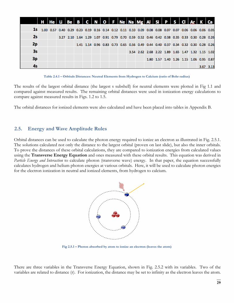
Table 2.4.1 – Orbitals Distances: Neutral Elements from Hydrogen to Calcium (ratio of Bohr radius)
The results of the largest orbital distance (the largest s subshell) for neutral elements were plotted in Fig 1.1 and compared against measured results. The remaining orbital distances were used in ionization energy calculations to compare against measured results in Figs. 1.2 to 1.5.
The orbital distances for ionized elements were also calculated and have been placed into tables in Appendix B.
2.5. Energy and Wave Amplitude Rules
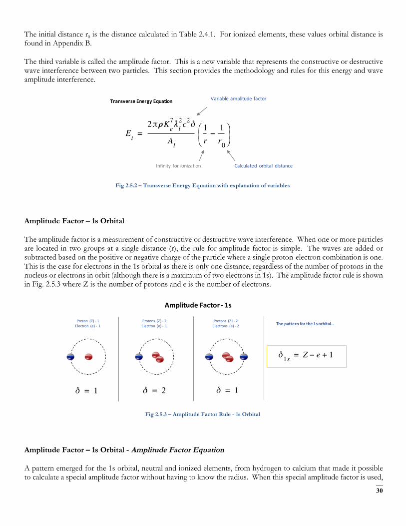
Orbital distances can be used to calculate the photon energy required to ionize an electron as illustrated in Fig. 2.5.1. The solutions calculated not only the distance to the largest orbital (proven on last slide), but also the inner orbitals. To prove the distances of these orbital calculations, they are compared to ionization energies from calculated values using the Transverse Energy Equation and ones measured with these orbital results. This equation was derived in Particle Energy and Interaction to calculate photon (transverse wave) energy. In that paper, the equation successfully calculates hydrogen and helium photon energies at various orbitals. Here, it will be used to calculate photon energies for the electron ionization in neutral and ionized elements, from hydrogen to calcium.
Fig 2.5.1 – Photon absorbed by atom to ionize an electron (leaves the atom)
There are three variables in the Transverse Energy Equation, shown in Fig. 2.5.2 with its variables. Two of the variables are related to distance (r). For ionization, the distance may be set to infinity as the electron leaves the atom.
30
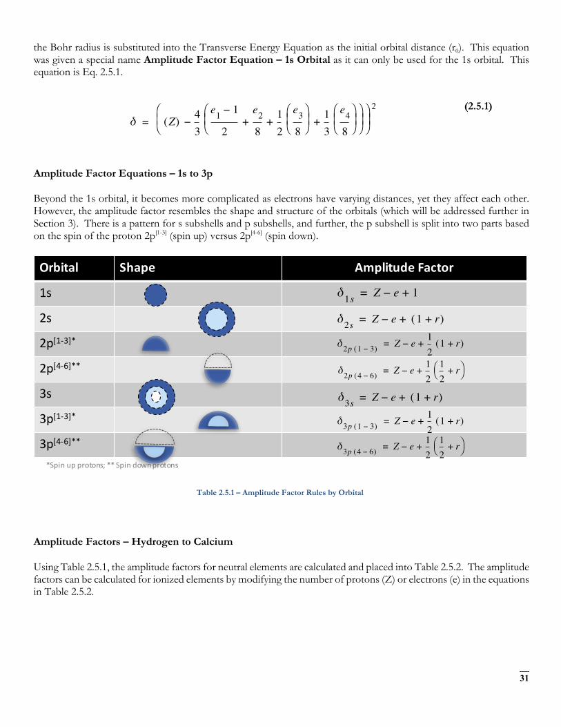
The initial distance r0 is the distance calculated in Table 2.4.1. For ionized elements, these values orbital distance is found in Appendix B.
The third variable is called the amplitude factor. This is a new variable that represents the constructive or destructive wave interference between two particles. This section provides the methodology and rules for this energy and wave amplitude interference.
Fig 2.5.2 – Transverse Energy Equation with explanation of variables
Amplitude Factor – 1s Orbital
The amplitude factor is a measurement of constructive or destructive wave interference. When one or more particles are located in two groups at a single distance (r), the rule for amplitude factor is simple. The waves are added or subtracted based on the positive or negative charge of the particle where a single proton-electron combination is one. This is the case for electrons in the 1s orbital as there is only one distance, regardless of the number of protons in the nucleus or electrons in orbit (although there is a maximum of two electrons in 1s). The amplitude factor rule is shown in Fig. 2.5.3 where Z is the number of protons and e is the number of electrons.
Fig 2.5.3 – Amplitude Factor Rule - 1s Orbital
Amplitude Factor – 1s Orbital - Amplitude Factor Equation
A pattern emerged for the 1s orbital, neutral and ionized elements, from hydrogen to calcium that made it possible to calculate a special amplitude factor without having to know the radius. When this special amplitude factor is used,
Et2π!Ke
7λl2c2δ
Al
1r
1r0
−⎝ ⎠⎜ ⎟⎛ ⎞=
Calculated orbital distanceInfinityforionization
VariableamplitudefactorTransverseEnergyEquation
AmplitudeFactor- 1s
Proton (Z)- 1Electron (e)- 1
Protons (Z)- 2Electron (e)- 1
Protons (Z)- 2Electrons (e)- 2
δ 1= δ 1=δ 2=
Thepatternforthe1sorbital…
δ1s Z e− 1+=
31
the Bohr radius is substituted into the Transverse Energy Equation as the initial orbital distance (r0). This equation was given a special name Amplitude Factor Equation – 1s Orbital as it can only be used for the 1s orbital. This equation is Eq. 2.5.1.
(2.5.1)
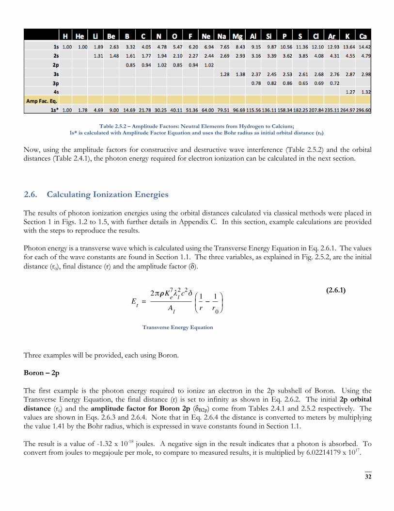
Amplitude Factor Equations – 1s to 3p
Beyond the 1s orbital, it becomes more complicated as electrons have varying distances, yet they affect each other. However, the amplitude factor resembles the shape and structure of the orbitals (which will be addressed further in Section 3). There is a pattern for s subshells and p subshells, and further, the p subshell is split into two parts based on the spin of the proton 2p[1-3] (spin up) versus 2p[4-6] (spin down).
Table 2.5.1 – Amplitude Factor Rules by Orbital
Amplitude Factors – Hydrogen to Calcium
Using Table 2.5.1, the amplitude factors for neutral elements are calculated and placed into Table 2.5.2. The amplitude factors can be calculated for ionized elements by modifying the number of protons (Z) or electrons (e) in the equations in Table 2.5.2.
δ Z( ) 43
e1 1−
2
e28
12
e38⎝ ⎠
⎜ ⎟⎛ ⎞ 1
3
e48⎝ ⎠
⎜ ⎟⎛ ⎞
+ + +⎝ ⎠⎜ ⎟⎛ ⎞
−⎝ ⎠⎜ ⎟⎛ ⎞ 2
=
Orbital Shape AmplitudeFactor
1s
2s
2p[1-3]*
2p[4-6]**
3s
3p[1-3]*
3p[4-6]**
*Spinupprotons;**Spindownprotons
δ1s Z e− 1+=
δ2s Z e− 1 r+( )+=
δ2p 1 3−( ) Z e− 121 r+( )+=
δ2p 4 6−( ) Z e− 1212
r+⎝ ⎠⎛ ⎞+=
δ3s Z e− 1 r+( )+=
δ3p 1 3−( ) Z e− 121 r+( )+=
δ3p 4 6−( ) Z e− 1212
r+⎝ ⎠⎛ ⎞+=
32
Table 2.5.2 – Amplitude Factors: Neutral Elements from Hydrogen to Calcium; 1s* is calculated with Amplitude Factor Equation and uses the Bohr radius as initial orbital distance (r0)
Now, using the amplitude factors for constructive and destructive wave interference (Table 2.5.2) and the orbital distances (Table 2.4.1), the photon energy required for electron ionization can be calculated in the next section.
2.6. Calculating Ionization Energies
The results of photon ionization energies using the orbital distances calculated via classical methods were placed in Section 1 in Figs. 1.2 to 1.5, with further details in Appendix C. In this section, example calculations are provided with the steps to reproduce the results.
Photon energy is a transverse wave which is calculated using the Transverse Energy Equation in Eq. 2.6.1. The values for each of the wave constants are found in Section 1.1. The three variables, as explained in Fig. 2.5.2, are the initial distance (r0), final distance (r) and the amplitude factor (δ).
Transverse Energy Equation
(2.6.1)
Three examples will be provided, each using Boron.
Boron – 2p
The first example is the photon energy required to ionize an electron in the 2p subshell of Boron. Using the Transverse Energy Equation, the final distance (r) is set to infinity as shown in Eq. 2.6.2. The initial 2p orbital distance (r0) and the amplitude factor for Boron 2p (δB2p) come from Tables 2.4.1 and 2.5.2 respectively. The values are shown in Eqs. 2.6.3 and 2.6.4. Note that in Eq. 2.6.4 the distance is converted to meters by multiplying the value 1.41 by the Bohr radius, which is expressed in wave constants found in Section 1.1.
The result is a value of -1.32 x 10⁻¹⁸ joules. A negative sign in the result indicates that a photon is absorbed. To convert from joules to megajoule per mole, to compare to measured results, it is multiplied by 6.02214179 x 10¹⁷.
Et2π!Ke
7λl2c2δ
Al
1r
1r0
−⎝ ⎠⎜ ⎟⎛ ⎞=
33
(2.6.2)
(2.6.3)
(2.6.4)
(2.6.5)
After converting from joules to megajoules per mole, the calculated result is -0.80 Mj/mol. This matches the measured result for Boron which is -.80 Mj/mol.13 Both values were charted in Fig. 1.2.
Boron – 1s
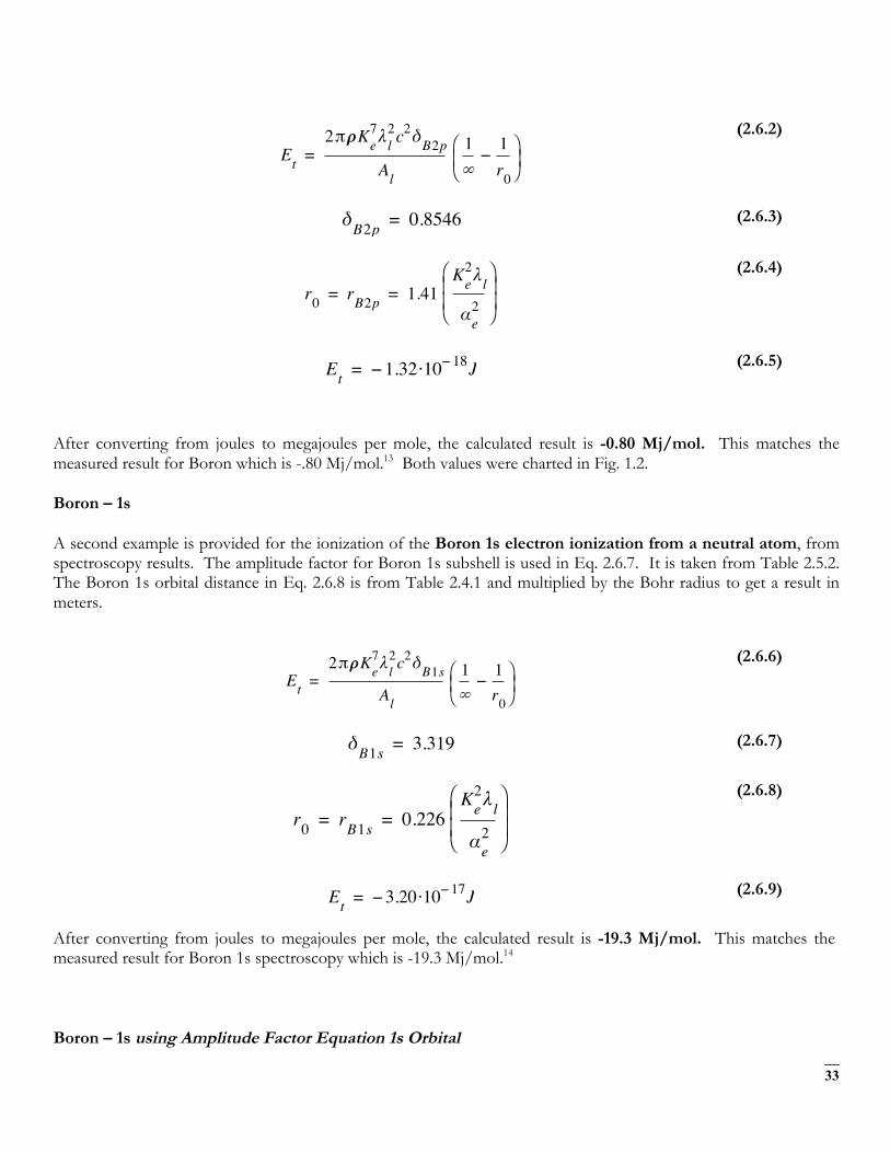
A second example is provided for the ionization of the Boron 1s electron ionization from a neutral atom, from spectroscopy results. The amplitude factor for Boron 1s subshell is used in Eq. 2.6.7. It is taken from Table 2.5.2. The Boron 1s orbital distance in Eq. 2.6.8 is from Table 2.4.1 and multiplied by the Bohr radius to get a result in meters.
(2.6.6)
(2.6.7)
(2.6.8)
(2.6.9)
After converting from joules to megajoules per mole, the calculated result is -19.3 Mj/mol. This matches the measured result for Boron 1s spectroscopy which is -19.3 Mj/mol.14
Boron – 1s using Amplitude Factor Equation 1s Orbital
Et2π!Ke
7λl2c2δB2pAl
1∞
1r0
−⎝ ⎠⎜ ⎟⎛ ⎞=
δB2p 0.8546=
r0 rB2p 1.41Ke2λl
αe2⎝ ⎠
⎜ ⎟⎜ ⎟⎛ ⎞
= =
Et 1.32 10 18− J·−=
Et2π!Ke
7λl2c2δB1sAl
1∞
1r0
−⎝ ⎠⎜ ⎟⎛ ⎞=
δB1s 3.319=
r0 rB1s 0.226Ke2λl
αe2⎝ ⎠
⎜ ⎟⎜ ⎟⎛ ⎞
= =
Et 3.20 10 17− J·−=
34
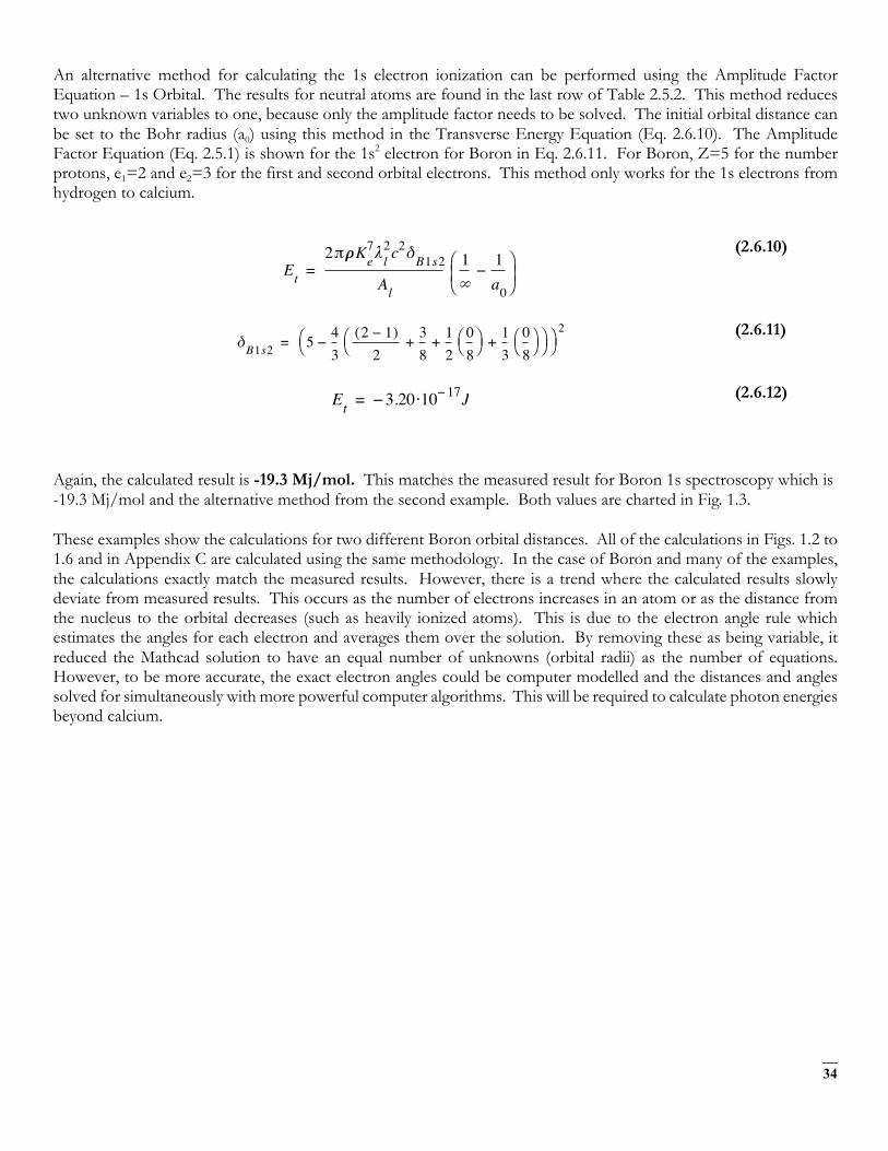
An alternative method for calculating the 1s electron ionization can be performed using the Amplitude Factor Equation – 1s Orbital. The results for neutral atoms are found in the last row of Table 2.5.2. This method reduces two unknown variables to one, because only the amplitude factor needs to be solved. The initial orbital distance can be set to the Bohr radius (a0) using this method in the Transverse Energy Equation (Eq. 2.6.10). The Amplitude Factor Equation (Eq. 2.5.1) is shown for the 1s2 electron for Boron in Eq. 2.6.11. For Boron, Z=5 for the number protons, e1=2 and e2=3 for the first and second orbital electrons. This method only works for the 1s electrons from hydrogen to calcium.
(2.6.10)
(2.6.11)
(2.6.12)
Again, the calculated result is -19.3 Mj/mol. This matches the measured result for Boron 1s spectroscopy which is -19.3 Mj/mol and the alternative method from the second example. Both values are charted in Fig. 1.3.
These examples show the calculations for two different Boron orbital distances. All of the calculations in Figs. 1.2 to 1.6 and in Appendix C are calculated using the same methodology. In the case of Boron and many of the examples, the calculations exactly match the measured results. However, there is a trend where the calculated results slowly deviate from measured results. This occurs as the number of electrons increases in an atom or as the distance from the nucleus to the orbital decreases (such as heavily ionized atoms). This is due to the electron angle rule which estimates the angles for each electron and averages them over the solution. By removing these as being variable, it reduced the Mathcad solution to have an equal number of unknowns (orbital radii) as the number of equations. However, to be more accurate, the exact electron angles could be computer modelled and the distances and angles solved for simultaneously with more powerful computer algorithms. This will be required to calculate photon energies beyond calcium.
Et2π!Ke
7λl2c2δB1s2Al
1∞
1a0
−⎝ ⎠⎜ ⎟⎛ ⎞=
δB1s2 5 43
2 1−( )2
38
1208⎝ ⎠
⎛ ⎞ 1308⎝ ⎠
⎛ ⎞+ + +⎝ ⎠⎛ ⎞−⎝ ⎠
⎛ ⎞ 2=
Et 3.20 10 17− J·−=
35
3. Orbital Shapes
Section 2 describes a method to calculate orbital distances, but it does not explain the strange shapes and probability nature of the electron. Using the proton’s pentaquark model, these shapes can be explained based on proton arrangement in an atomic nucleus.
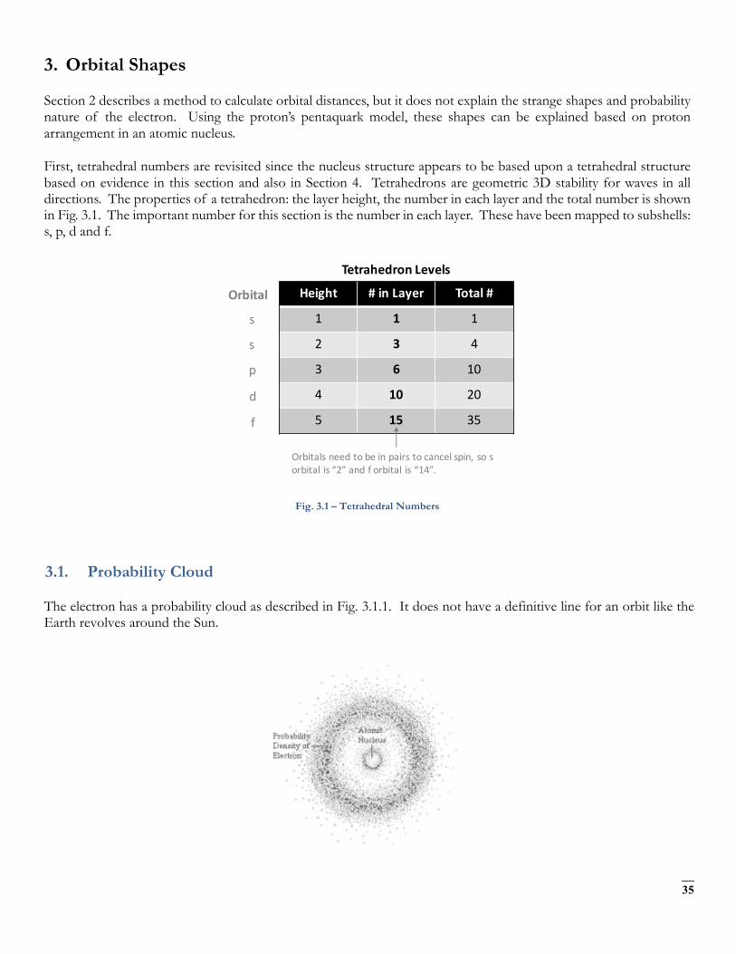
First, tetrahedral numbers are revisited since the nucleus structure appears to be based upon a tetrahedral structure based on evidence in this section and also in Section 4. Tetrahedrons are geometric 3D stability for waves in all directions. The properties of a tetrahedron: the layer height, the number in each layer and the total number is shown in Fig. 3.1. The important number for this section is the number in each layer. These have been mapped to subshells: s, p, d and f.
Fig. 3.1 – Tetrahedral Numbers
3.1. Probability Cloud
The electron has a probability cloud as described in Fig. 3.1.1. It does not have a definitive line for an orbit like the Earth revolves around the Sun.
Height #inLayer Total#
1 1 1
2 3 4
3 6 10
4 10 20
5 15 35
TetrahedronLevels
Orbital
s
s
p
d
f
Orbitalsneedtobeinpairstocancelspin, sosorbitalis“2”andforbitalis“14”.
36
Fig. 3.1.1 – Electron Probability Cloud 15
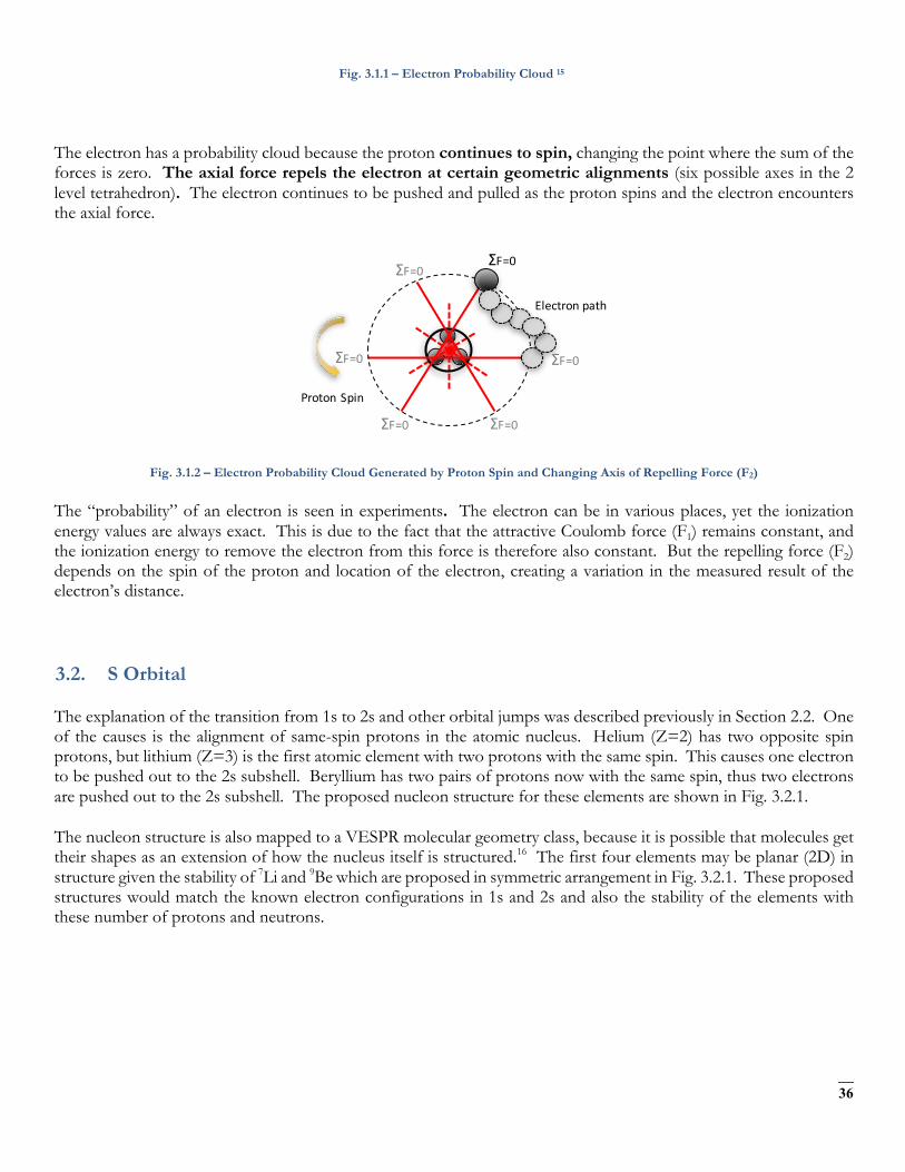
The electron has a probability cloud because the proton continues to spin, changing the point where the sum of the forces is zero. The axial force repels the electron at certain geometric alignments (six possible axes in the 2 level tetrahedron). The electron continues to be pushed and pulled as the proton spins and the electron encounters the axial force.
Fig. 3.1.2 – Electron Probability Cloud Generated by Proton Spin and Changing Axis of Repelling Force (F2)
The “probability” of an electron is seen in experiments. The electron can be in various places, yet the ionization energy values are always exact. This is due to the fact that the attractive Coulomb force (F1) remains constant, and the ionization energy to remove the electron from this force is therefore also constant. But the repelling force (F2) depends on the spin of the proton and location of the electron, creating a variation in the measured result of the electron’s distance.
3.2. S Orbital
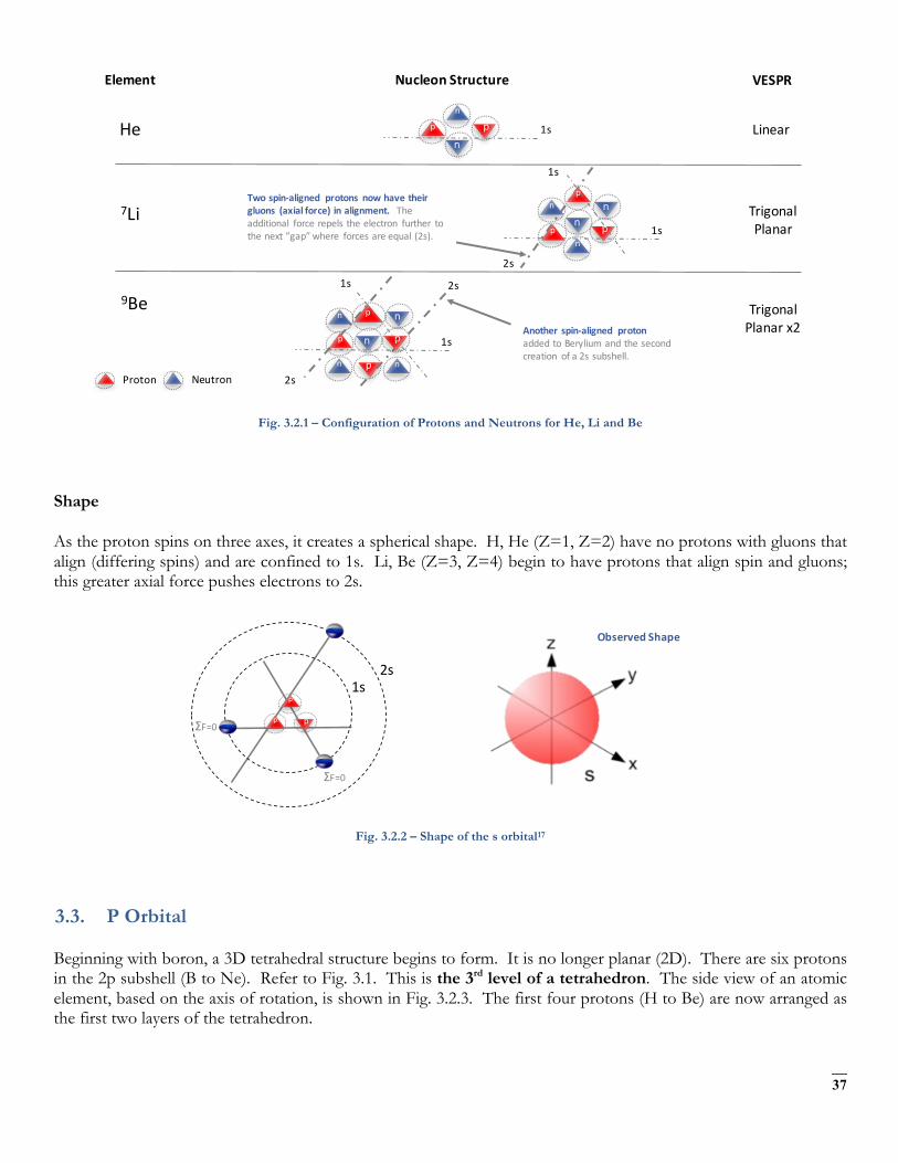
The explanation of the transition from 1s to 2s and other orbital jumps was described previously in Section 2.2. One of the causes is the alignment of same-spin protons in the atomic nucleus. Helium (Z=2) has two opposite spin protons, but lithium (Z=3) is the first atomic element with two protons with the same spin. This causes one electron to be pushed out to the 2s subshell. Beryllium has two pairs of protons now with the same spin, thus two electrons are pushed out to the 2s subshell. The proposed nucleon structure for these elements are shown in Fig. 3.2.1.
The nucleon structure is also mapped to a VESPR molecular geometry class, because it is possible that molecules get their shapes as an extension of how the nucleus itself is structured.16 The first four elements may be planar (2D) in structure given the stability of 7Li and 9Be which are proposed in symmetric arrangement in Fig. 3.2.1. These proposed structures would match the known electron configurations in 1s and 2s and also the stability of the elements with these number of protons and neutrons.
Electronpath
ΣF=0
ΣF=0
ΣF=0
ΣF=0
ΣF=0 ΣF=0ProtonSpin
37
Fig. 3.2.1 – Configuration of Protons and Neutrons for He, Li and Be
Shape
As the proton spins on three axes, it creates a spherical shape. H, He (Z=1, Z=2) have no protons with gluons that align (differing spins) and are confined to 1s. Li, Be (Z=3, Z=4) begin to have protons that align spin and gluons; this greater axial force pushes electrons to 2s.
Fig. 3.2.2 – Shape of the s orbital17
3.3. P Orbital
Beginning with boron, a 3D tetrahedral structure begins to form. It is no longer planar (2D). There are six protons in the 2p subshell (B to Ne). Refer to Fig. 3.1. This is the 3rd level of a tetrahedron. The side view of an atomic element, based on the axis of rotation, is shown in Fig. 3.2.3. The first four protons (H to Be) are now arranged as the first two layers of the tetrahedron.
Element NucleonStructure VESPR
Proton Neutron
p
n
He
7Li
9Be
pn
1s Linear
TrigonalPlanar
TrigonalPlanarx2
pn
p 1spn
n
n
1s
2s
pn
p 1sp n
n
n
1s
2sn p
2s
Twospin-aligned protons nowhavetheirgluons (axialforce)inalignment. Theadditional forcerepelstheelectron further tothenext”gap”where forcesareequal(2s).
Anotherspin-aligned protonaddedtoBerylium andthesecondcreation ofa2ssubshell.
ΣF=0
p
ppΣF=0
2s1s
ObservedShape
38
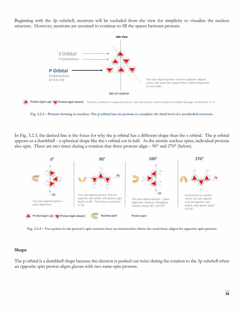
Beginning with the 2p subshell, neutrons will be excluded from the view for simplicity to visualize the nucleus structure. However, neutrons are assumed to continue to fill the spaces between protons.
Fig. 3.2.3 – Protons forming in nucleus. The p orbital has six protons to complete the third level of a tetrahedral structure.
In Fig. 3.2.3, the dashed line is the focus for why the p orbital has a different shape than the s orbital. The p orbital appears as a dumbbell – a spherical shape like the s orbital cut in half. As the atomic nucleus spins, individual protons also spin. There are two times during a rotation that three protons align – 90° and 270° (below).
Fig. 3.2.4 – Two points in the proton’s spin rotation have an intersection where the axial force aligns for opposite spin protons
Shape
The p orbital is a dumbbell shape because the electron is pushed out twice during the rotation to the 3p subshell when an opposite spin proton aligns gluons with two same-spin protons.
Neutrons continue toseparateprotons, butonlyprotons willbeshowntosimplifydrawingsofelementsZ>4.Proton(spinup) Proton(spindown)
Axisofrotation
SideView
POrbital6totalprotons(Z=5to10)
S Orbital4 totalprotons
Twospin-alignedprotons andoneopposite alignedproton willcausetheshapeoftheporbital (explainedonnextslide)
Proton(spinup) Proton(spindown)
2p
0°
Twospin-alignedprotons –gluonalignment.
Nucleusspin Protonspin
90° 180° 270°
3p
Twospin-alignedprotons andoneopposite spinproton withgluonsalignbrieflyat90°. Thisforcesanelectronto3p.
Secondtimeinrotationwheretwospin-alignedandoneopposite spinproton aligngluonsagainat270°.
Twospin-alignedprotons – gluonalignmentcontinues throughoutrotation except 90° and270°.
2p
3p

39
Fig. 3.2.5 – Dumbbell shape of p orbital due to two points in rotation where sum of forces is not at 2p distance
Proton Fill Order
Protons with spins aligned with the atomic nucleus’ spin will fill first as there is less energy required before a proton with opposite spin is filled in the nucleus structure. Protons also fill from the center then outwards for geometric stability. Fig. 3.2.6 shows the fill order of atomic elements from boron (B) to neon (Ne) in both the side view of the nucleus and the bottom row (third row) which is being filled with protons.
Fig. 3.2.6 – Fill order of p orbital electrons (side view and bottom view shown)
3.4. D Orbital
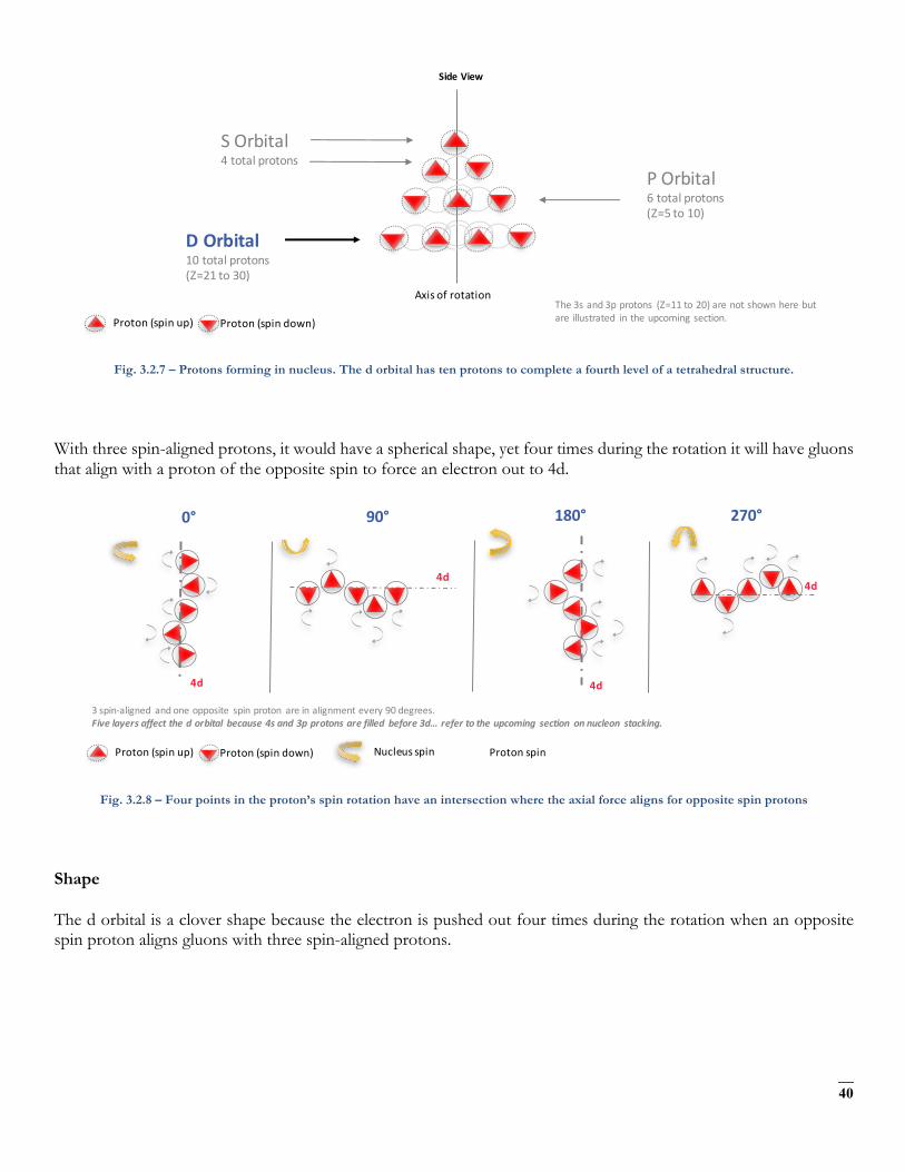
The d orbital contains 10 electrons. Again, refer to Fig. 3.1. This is the 4th level of the tetrahedron. This is illustrated in Fig. 3.2.7. Note that the 3s and 3p protons are not shown in this tetrahedral view, but are addressed in Section 4.
ΣF!=0
2p
ΣF=0
ΣF=0
ObservedShape
Topview oftetrahedronstructure anditssideplanesthathavetheproton alignmentasthestructure spins.
90°270°
ΣF=0 y-z
x-y
x-z
3p
Sumofforcesatthe2porbitaldistanceisnotzero,leavingagapastheelectron isforcedoutat90° and270°.
Element
OtoNe(Z=8to10)
BtoN(Z=5to7)
SideView BottomView(3rd Row)
Proton(spinup) Proton(spindown)
Spinupprotons fillcenter ofthird rowfirstforgeometric stability.
Spindownprotons filltheoutside tocomplete the3rdrowoftetrahedron.
40
Fig. 3.2.7 – Protons forming in nucleus. The d orbital has ten protons to complete a fourth level of a tetrahedral structure.
With three spin-aligned protons, it would have a spherical shape, yet four times during the rotation it will have gluons that align with a proton of the opposite spin to force an electron out to 4d.
Fig. 3.2.8 – Four points in the proton’s spin rotation have an intersection where the axial force aligns for opposite spin protons
Shape
The d orbital is a clover shape because the electron is pushed out four times during the rotation when an opposite spin proton aligns gluons with three spin-aligned protons.
Proton(spinup) Proton(spindown)
Axisofrotation
SideView
POrbital6totalprotons(Z=5to10)
S Orbital4 totalprotons
D Orbital10totalprotons(Z=21to30)
The3sand3pprotons (Z=11to20)arenotshownherebutareillustrated intheupcomingsection.
Proton(spinup) Proton(spindown)
4d
0°
3spin-aligned andoneopposite spinproton areinalignment every90degrees.Fivelayersaffectthedorbital because4sand3pprotonsarefilled before3d… refertotheupcoming section onnucleon stacking.
Nucleusspin Protonspin
90° 180° 270°
4d
4d
4d

41
Fig. 3.2.9 – Dumbbell shape of d orbital due to four points in rotation where sum of forces is not at 3d distance
Proton Fill Order
At Z=21, scandium (Sc) is the first element that begins a d orbital. As protons always build from the center then outwards for stability, the first proton is placed in the center (refer to Fig. 3.2.10). In a 4th row of a tetrahedron, this is the first time that a unit is in the center of axis of rotation. This creates a unique shape relative to other d orbital shapes (refer to shape highlighted in yellow).
Fig. 3.2.10 – Fill order of the 1st d orbital electron (bottom view shown)
The next three elements build outwards from the center, occupying the three sides of the triangle as shown below. These now have the clover shape as there are four points in the rotation where the repelling, axial force distance changes as shown in Fig 3.2.9. These take place on the x-y, x-z and y-z planes of the tetrahedron while it spins. This is highlighted in yellow below.
ObservedShape
ΣF!=0
3d
ΣF=0
90°270°ΣF=0
4d
0°
180°Nowthereare fourtimesduringtherotationwhere thesumofforcesisnotzeroatthe3dorbitaldistanceandtheelectronisforcedfurtherout.
Sc(Z=21)
BottomView(4thRow)
Proton(spinup) Proton(spindown)
y-z
x-y
x-z
Thisisthefirstproton inatetrahedral structure thatisalignedwiththetopproton ontheaxisofrotation (zaxis).Asaresult, ithasaunique shape.
42
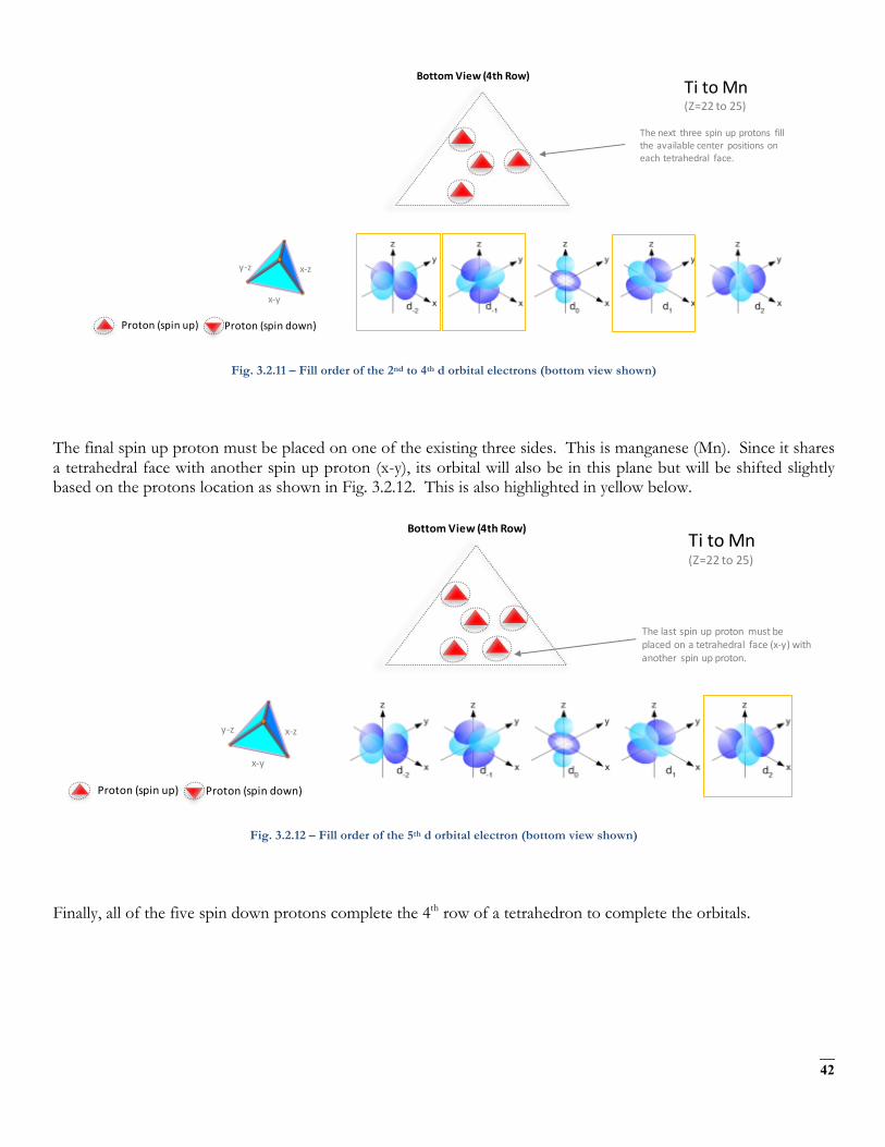
Fig. 3.2.11 – Fill order of the 2nd to 4th d orbital electrons (bottom view shown)
The final spin up proton must be placed on one of the existing three sides. This is manganese (Mn). Since it shares a tetrahedral face with another spin up proton (x-y), its orbital will also be in this plane but will be shifted slightly based on the protons location as shown in Fig. 3.2.12. This is also highlighted in yellow below.
Fig. 3.2.12 – Fill order of the 5th d orbital electron (bottom view shown)
Finally, all of the five spin down protons complete the 4th row of a tetrahedron to complete the orbitals.
Ti toMn(Z=22to25)
BottomView(4thRow)
Proton(spinup) Proton(spindown)
y-z
x-y
x-z
Thenext threespinupprotons filltheavailablecenter positionsoneachtetrahedral face.
Ti toMn(Z=22to25)
BottomView(4thRow)
Proton(spinup) Proton(spindown)
y-z
x-y
x-z
Thelastspinupproton mustbeplacedonatetrahedral face(x-y)withanother spinupproton.

43
Fig. 3.2.13 – Fill order of the spin down orbital electrons (bottom view shown)
3.5. F Orbital
The sequence for the f block is unique. Beginning with lanthanum (Z=57) it starts a block that contains 15 elements. Again, refer to Fig. 3.1. The 5th level of a tetrahedron has 15 units. There are 15 elements for the f block (Z=57 to 71), although an odd number affects the number of orbitals (14 / 2 = 7). It converts a proton to neutron in the next d block to compensate, beginning with the 5d block.
Fig. 3.2.14 – Protons forming in nucleus. The f orbital has 15 protons to complete a fifth level of a tetrahedral structure.
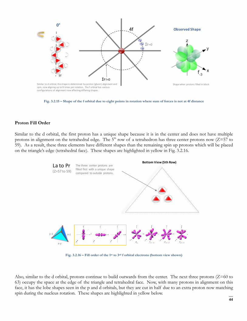
Shape
The f orbital is more complex, but follows the same rules based on proton alignment as the p and d orbitals. When completely full it is similar to the d orbital, but cut in half (eight lobes instead of four). It is based on the points in the nucleus rotation where the gluons of opposite spin protons align.
BottomView(4thRow)
Proton(spinup) Proton(spindown)
y-z
x-y
x-z
FetoZn(Z=26to30)
Finally,thefivespindown protonscomplete thebottomlayerofthe4th rowofatetrahedron.
Proton(spinup) Proton(spindown) Axisofrotation
SideView
POrbital6totalprotons(Z=5to10)
S Orbital4 totalprotons
F Orbital15totalprotons(Z=57to71)
DOrbital10totalprotons(Z=21to30)
Theother sandporbital protons arenotshown
herebutareillustrated intheupcomingsection.
44
Fig. 3.2.15 – Shape of the f orbital due to eight points in rotation where sum of forces is not at 4f distance
Proton Fill Order
Similar to the d orbital, the first proton has a unique shape because it is in the center and does not have multiple protons in alignment on the tetrahedral edge. The 5th row of a tetrahedron has three center protons now (Z=57 to 59). As a result, these three elements have different shapes than the remaining spin up protons which will be placed on the triangle’s edge (tetrahedral face). These shapes are highlighted in yellow in Fig. 3.2.16.
Fig. 3.2.16 – Fill order of the 1st to 3rd f orbital electrons (bottom view shown)
Also, similar to the d orbital, protons continue to build outwards from the center. The next three protons (Z=60 to 63) occupy the space at the edge of the triangle and tetrahedral face. Now, with many protons in alignment on this face, it has the lobe shapes seen in the p and d orbitals, but they are cut in half due to an extra proton now matching spin during the nucleus rotation. These shapes are highlighted in yellow below.
ObservedShape
5f
0°
ShapewhenprotonsfilledinblockSimilar todorbital,theshapeisdeterminedbyproton(gluon)alignmentandspin,nowaligningupto8timesperrotation.Theforbitalhasvariousconfigurationsofalignmentnowaffectingdifferingshapes.
ΣF!=0
4f
ΣF=0
LatoPr(Z=57to59)
BottomView(5thRow)
y-z
x-y
x-z
Thethree centerprotons arefilledfirst withauniqueshapecompared tooutside protons.

45
Fig. 3.2.17 – Fill order of the 4th to 6th f orbital electrons (bottom view shown)
Once again, similar to the d orbital, the last spin up proton must be placed on one of the three triangular edges. It will share an edge with an existing x-y spin up proton, but the orbital is shifted on this plane because of the location of the proton.
Fig. 3.2.18 – Fill order of the 7th f orbital electron (bottom view shown)
Finally, seven spin down protons are added to the 5th row of a tetrahedral structure to complete the orbitals. There are now 7 spin up and 7 spin down protons. This matches the orbitals seen in the f series. However, there is one more space in the 5th row of a tetrahedron because it has 15 units. One last proton completes this row and it causes the next d block series to have 9 elements. This is confirmed in the Periodic Table of Elements as the 5d block (Z=72 to 80) contains 9 elements. In addition, the transition from 4f to 5d and again from 5f to 6d shows a mass increase
Nd toEu(Z=60to63)
BottomView(5thRow)
y-z
x-y
x-z
Thenext threespinupprotons filltheavailablecenter positionsoneachtetrahedral face.
Nd toEu(Z=60to63)
BottomView(5thRow)
y-z
x-y
x-z
Thelastspinupproton mustbeplacedonatetrahedral facewithanother spinupproton.

46
that includes at least three neutrons before the next element. This means that the d block has a neutron take the position of a proton so that it can have 9 protons in a row, otherwise it requires 10 units to complete a row (two of the three neutrons are separation neutrons and the third occupies the proton’s position).
Fig. 3.2.19 – Fill order of the remaining f orbital electrons (bottom view shown)
Using the same rules that enabled the calculations of orbital distances in Section 2, specifically that the proton is a pentaquark with gluons that align to cause a repelling force, the probability nature and shape of orbitals can be logically explained. The shapes match a nucleus structure that is based on a tetrahedral sequence. This nucleus structure is then further validated by the atomic element sequence seen in the Periodic Table of Elements, described in more detail in the next section.
BottomView(5thRow)
y-z
x-y
x-z
Gd toLu(Z=64to71)
Sevenspindownprotons matchthesevenspinupprotons tofilltheorbitals.
Thelastremainingproton completes thebottom layerofthe5th rowofatetrahedron(15),howeverthisisanoddnumberandcannotbeanorbital becauseanorbitalrequires twoelectrons ofopposite spin.
Itwillreduce aproton fromthenextdorbitaltocomplete byputtinganeutron inplaceofaproton. Thisisseenintheatomicmassincreasesbetween4fand5dblocksandalso5fto6dblocks(174.9to178.5amu and262to267amu respectivelyduetomassincreasesforatleastthreeneutrons beforethenextproton).
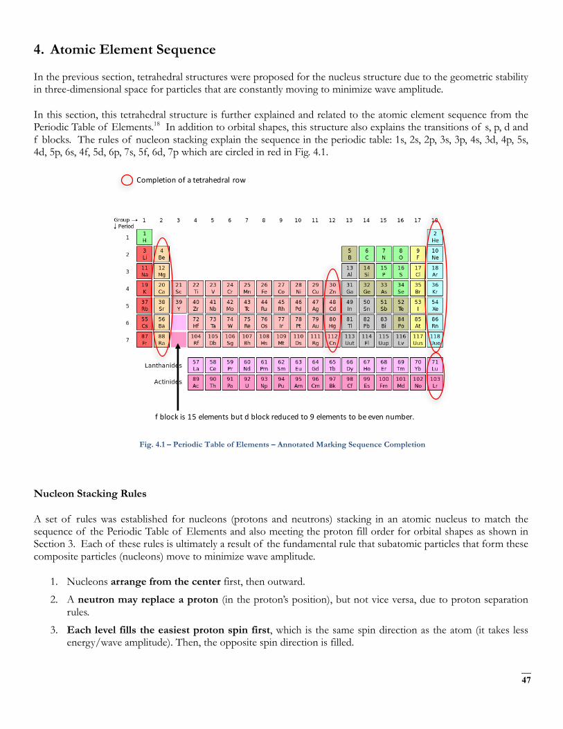
47
4. Atomic Element Sequence
In the previous section, tetrahedral structures were proposed for the nucleus structure due to the geometric stability in three-dimensional space for particles that are constantly moving to minimize wave amplitude.
In this section, this tetrahedral structure is further explained and related to the atomic element sequence from the Periodic Table of Elements.18 In addition to orbital shapes, this structure also explains the transitions of s, p, d and f blocks. The rules of nucleon stacking explain the sequence in the periodic table: 1s, 2s, 2p, 3s, 3p, 4s, 3d, 4p, 5s, 4d, 5p, 6s, 4f, 5d, 6p, 7s, 5f, 6d, 7p which are circled in red in Fig. 4.1.
Fig. 4.1 – Periodic Table of Elements – Annotated Marking Sequence Completion
Nucleon Stacking Rules
A set of rules was established for nucleons (protons and neutrons) stacking in an atomic nucleus to match the sequence of the Periodic Table of Elements and also meeting the proton fill order for orbital shapes as shown in Section 3. Each of these rules is ultimately a result of the fundamental rule that subatomic particles that form these composite particles (nucleons) move to minimize wave amplitude.
1. Nucleons arrange from the center first, then outward.
2. A neutron may replace a proton (in the proton’s position), but not vice versa, due to proton separation rules.
3. Each level fills the easiest proton spin first, which is the same spin direction as the atom (it takes less energy/wave amplitude). Then, the opposite spin direction is filled.
f blockis15elementsbutdblockreducedto9elementstobeevennumber.
Completionofatetrahedral row
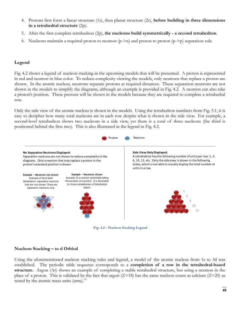
48
4. Protons first form a linear structure (1s), then planar structure (2s), before building in three dimensions in a tetrahedral structure (2p).
5. After the first complete tetrahedron (2p), the nucleons build symmetrically - a second tetrahedron.
6. Nucleons maintain a required proton to neutron (p->n) and proton to proton (p->p) separation rule.
Legend
Fig. 4.2 shows a legend of nucleon stacking in the upcoming models that will be presented. A proton is represented in red and neutron in blue color. To reduce complexity viewing the models, only neutrons that replace a proton are shown. In the atomic nucleus, neutrons separate protons at required distances. These separation neutrons are not shown in the models to simplify the diagrams, although an example is provided in Fig. 4.2. A neutron can also take a proton’s position. These protons will be shown in the models because they are required to complete a tetrahedral row.
Only the side view of the atomic nucleus is shown in the models. Using the tetrahedron numbers from Fig. 3.1, it is easy to decipher how many total nucleons are in each row despite what is shown in the side view. For example, a second-level tetrahedron shows two nucleons in a side view, yet there is a total of three nucleons (the third is positioned behind the first two). This is also illustrated in the legend in Fig. 4.2.
Fig. 4.2 – Nucleon Stacking Legend
Nucleon Stacking – to d Orbital
Using the aforementioned nucleon stacking rules and legend, a model of the atomic nucleus from 1s to 3d was established. The periodic table sequence corresponds to a completion of a row in the tetrahedral-based structure. Argon (Ar) shows an example of completing a stable tetrahedral structure, but using a neutron in the place of a proton. This is validated by the fact that argon (Z=18) has the same nucleon count as calcium (Z=20) as noted by the atomic mass units (amu).19
13
610
15
Proton Neutron
Example– NeutronsnotshownExampleofthirdlevel
tetrahedronseparationneutronsthatarenotshown.Theseareseparationneutronsonly.
NoSeparationNeutronsDisplayed:Separationneutronsarenotshowntoreducecomplexityinthediagrams.Onlyaneutronthatmayreplaceaprotonintheproton’sstandardpositionisshown.
Example– NeutronsshownExampleofaneutronpotentiallytakingthepositionofaproton.Itisillustratedtoshowcompletenessoftetrahedral
object.
SideViewOnlyDisplayed:Atetrahedronhasthefollowingnumberofunitsperrow:1,3,6,10,15,etc.Onlythesideviewisshowninthefollowingslides,whichisnotabletovisuallydisplaythetotalnumberofunitsinarow.

49
Fig. 4.3 – Nucleon Stacking from 1s to 3d Atomic Elements (He to Zn)
Nucleon Stacking – to f Orbital (potential arrangement)
The nucleon stacking model was continued through the first f orbital (Hg), although the variations and possibilities for symmetry become more complex. Thus, these models are potential arrangements that match the nucleon stacking rules to keep symmetry and stability in the nucleus when it corresponds to the end of a block sequence.
Fig. 4.4 – Nucleon Stacking from 4p to 4f Atomic Elements (Kr to Hg)
1s(He)
2protons
Linear TrigonalPlanar
2s(Be)
4 protons
Tetrahedral
2p(Ne)
10protons
3s(Mg)
12protons
3p(Ar)
18protons
4s(Ca)
20protons
3d(Zn)
30protons
Linear structureaddedtotetrahedral structureassecondtetrahedronbeginstobuildsymmetrically.
Second3rd row(porbital)added.Ar has39.948amu,samenucleoncountasCa(40).Twoneutronsfillthevoidoftwoprotons.
Twocompletetetrahedrons.Cahas40.078amu,samenucleoncountasAr(40).Protonsreplacethetwoneutrons.
4p(Kr)
36protons
5s(Sr)
38protons
4d(Cd)
48protons
5p(Xe)
54protons
6s(Ba)
56protons
4f(Hg)
80protons
Sixprotonsaddedasportbital.Krhas83.798amu,whichissufficientforanadditionalsixneutronsthatcouldmakeanotherprow(notpictured).
Linear (sorbital)rowadded.2protons.
10protonsaddedforanotherdorbitalrow.
6 protonsaddedforanotherporbitalrow. Possiblethataneutronmay resideinaproton’spositioninthesrow.
2protonsaddedforanothersorbitalrow.Possiblethataneutronmay resideinaproton’spositioninthesrow.
15protonsaddedfortheforbitalrow.Oneprotonwillberemovedfromthenextdrowtocompensate.
50
5. Conclusion
Atomic orbitals and the behavior of the electron in the presence of an atomic nuclei consisting of one or more protons can be calculated and explained using classical mechanics equations for forces. Specifically, the resting position of the electron is based on the point where the attractive and repulsive forces are equal – known as the point where the sum of the forces is zero.
This required a different model of the proton that originated with the Forces paper that accurately modeled the strong force. The repulsive force is the effect of two quarks in alignment, which produces a strong, axial attraction when within standing wave distance, but is a repelling force beyond these standing waves. This repulsive force is what causes the electron to stay at a distance from the nucleus that becomes the orbital. It also has an attractive force due to the anti-quark (or positron) in the center of the proton. Because there are distinct points in the proton’s spin where the electron experiences this outward, axial force, the electron is constantly being pushed and pulled by the nucleus. This four-quark and one anti-quark configuration of the proton has recently been observed in pentaquark experiments.
After manually calculating the distances for hydrogen and helium and establishing a set of rules and equations, elements beyond lithium required greater computational power to simultaneously solve multiple equations and unknowns as electrons reside in two or more orbital distances. Using Mathcad, orbital distances were solved for elements up to the 4s subshell (calcium), which required computing six equations and six unknowns simultaneously. Elements greater than calcium may be computed in the future with enhanced computer modeling, which will also require better methods for determining specific electron angles.
The orbital distances were compared to measured results of atomic distances and were within reasonable accuracy (exact measurements of atomic orbitals are difficult due to the constantly changing electron’s position). Twenty comparisons were charted in Fig. 1.1 for orbital distances. A second method was selected to validate orbital distance that allowed a greater number of comparisons. More than 150 comparisons of calculated ionization energies versus measured energies were provided in Figs. 1.2 to 1.6. This method was chosen as a second validation because orbital distance is required in the calculation of ionization energy.
A classical explanation of the electron’s orbit and a pentaquark model of the proton also provides an explanation for the probability cloud of the electron and the shape of the orbital, including quantum leaps. These shapes and leaps are based on the arrangement of the axial force from proton alignment. This led to modeling of the atomic nucleus to explain the exact shape of each orbital and the sequence of the Periodic Table of Elements. The structure is linear for the first two elements (H and He), triangular planar for the next two elements (Li and Be) and then tetrahedral for the remaining elements beginning with boron (B).
The Particle Energy and Interaction and Forces papers also showed tetrahedral patterns for the electron and proton. Although experiments have observed that molecules have triangular and tetrahedral structures, atomic nuclei and subatomic particles are not observed directly and their structure must be deduced from other observations. There is enough evidence across these papers that a single, fundamental particle builds structures from the electron (particle) to the proton (composite particle) to an atomic nucleus (element) to molecules. All of these are based on a stable formation of a fundamental particle that reacts to waves in all three dimensions and minimizes its wave amplitude. This is illustrated in Fig. 5.1.
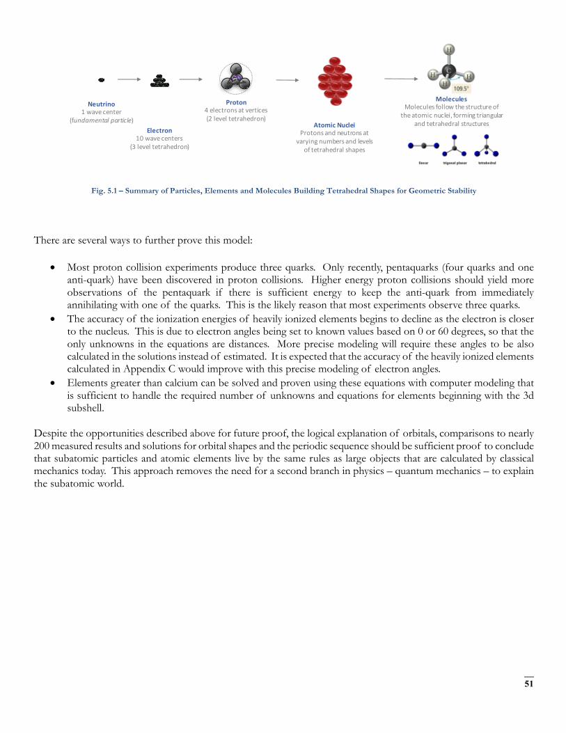
51
Fig. 5.1 – Summary of Particles, Elements and Molecules Building Tetrahedral Shapes for Geometric Stability
There are several ways to further prove this model:
• Most proton collision experiments produce three quarks. Only recently, pentaquarks (four quarks and one anti-quark) have been discovered in proton collisions. Higher energy proton collisions should yield more observations of the pentaquark if there is sufficient energy to keep the anti-quark from immediately annihilating with one of the quarks. This is the likely reason that most experiments observe three quarks.
• The accuracy of the ionization energies of heavily ionized elements begins to decline as the electron is closer to the nucleus. This is due to electron angles being set to known values based on 0 or 60 degrees, so that the only unknowns in the equations are distances. More precise modeling will require these angles to be also calculated in the solutions instead of estimated. It is expected that the accuracy of the heavily ionized elements calculated in Appendix C would improve with this precise modeling of electron angles.
• Elements greater than calcium can be solved and proven using these equations with computer modeling that is sufficient to handle the required number of unknowns and equations for elements beginning with the 3d subshell.
Despite the opportunities described above for future proof, the logical explanation of orbitals, comparisons to nearly 200 measured results and solutions for orbital shapes and the periodic sequence should be sufficient proof to conclude that subatomic particles and atomic elements live by the same rules as large objects that are calculated by classical mechanics today. This approach removes the need for a second branch in physics – quantum mechanics – to explain the subatomic world.
Electron10wavecenters
(3leveltetrahedron)
Proton4electronsatvertices(2leveltetrahedron)
AtomicNucleiProtonsandneutronsat
varyingnumbersandlevelsoftetrahedralshapes
MoleculesMoleculesfollowthestructureof
theatomicnuclei,formingtriangularandtetrahedralstructures
Neutrino1wavecenter
(fundamentalparticle)

52
Acknowledgements
The authors acknowledge the support from National Key Research and Development Program of China (2016YFB0401501), the National Natural Science Foundation of China (Grant No. 51561135014, Guangdong Innovative Research Team Program (No. 2011D039), the Program for Changjiang Scholars, Innovative Research Teams in Universities Project (No. IRT13064), Science and technology project of Guangdong Province (No. 2016B090918083), the 111 project and Guangzhou Key Laboratory of Electronic Paper Displays Materials and Devices (201705030007).
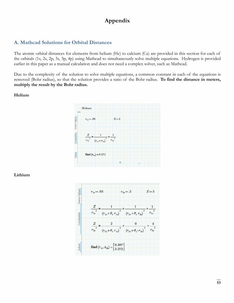
53
Appendix
A. Mathcad Solutions for Orbital Distances
The atomic orbital distances for elements from helium (He) to calcium (Ca) are provided in this section for each of the orbitals (1s, 2s, 2p, 3s, 3p, 4p) using Mathcad to simultaneously solve multiple equations. Hydrogen is provided earlier in this paper as a manual calculation and does not need a complex solver, such as Mathcad.
Due to the complexity of the solution to solve multiple equations, a common constant in each of the equations is removed (Bohr radius), so that the solution provides a ratio of the Bohr radius. To find the distance in meters, multiply the result by the Bohr radius.
Helium
Lithium
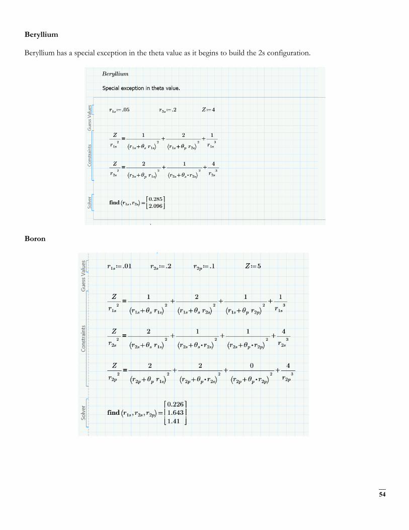
54
Beryllium
Beryllium has a special exception in the theta value as it begins to build the 2s configuration.
Boron
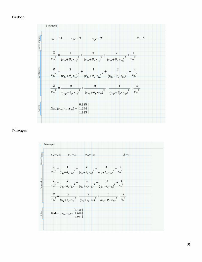
55
Carbon
Nitrogen

56
Oxygen
Flourine
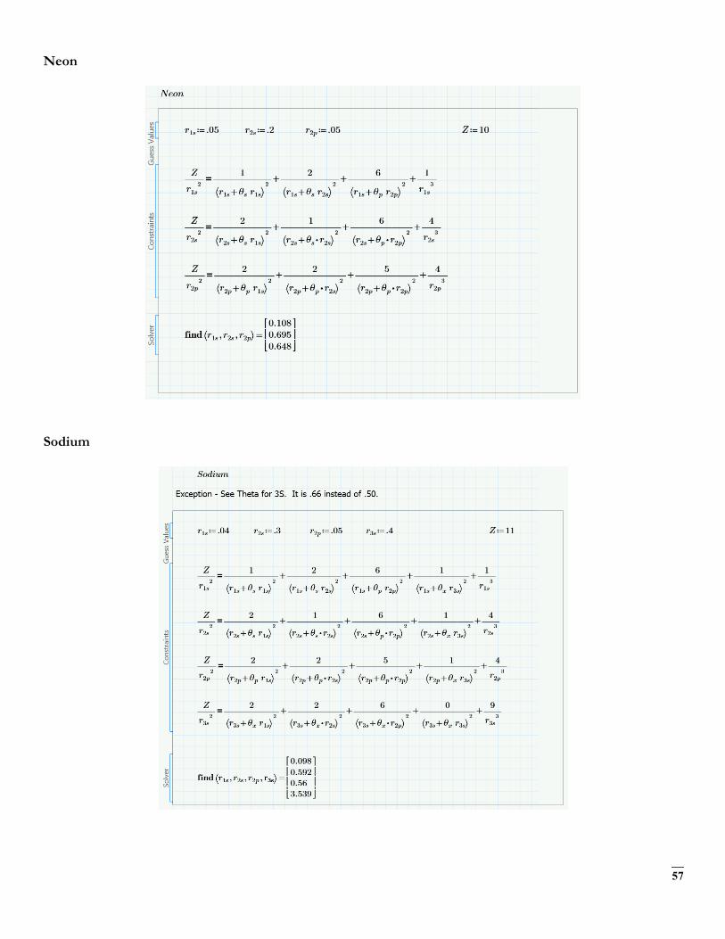
57
Neon
Sodium
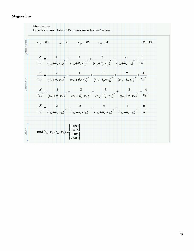
58
Magnesium

59
Aluminum
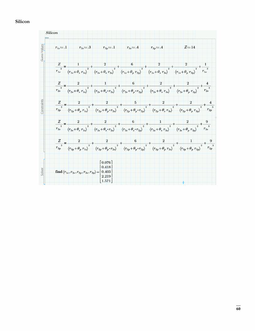
60
Silicon
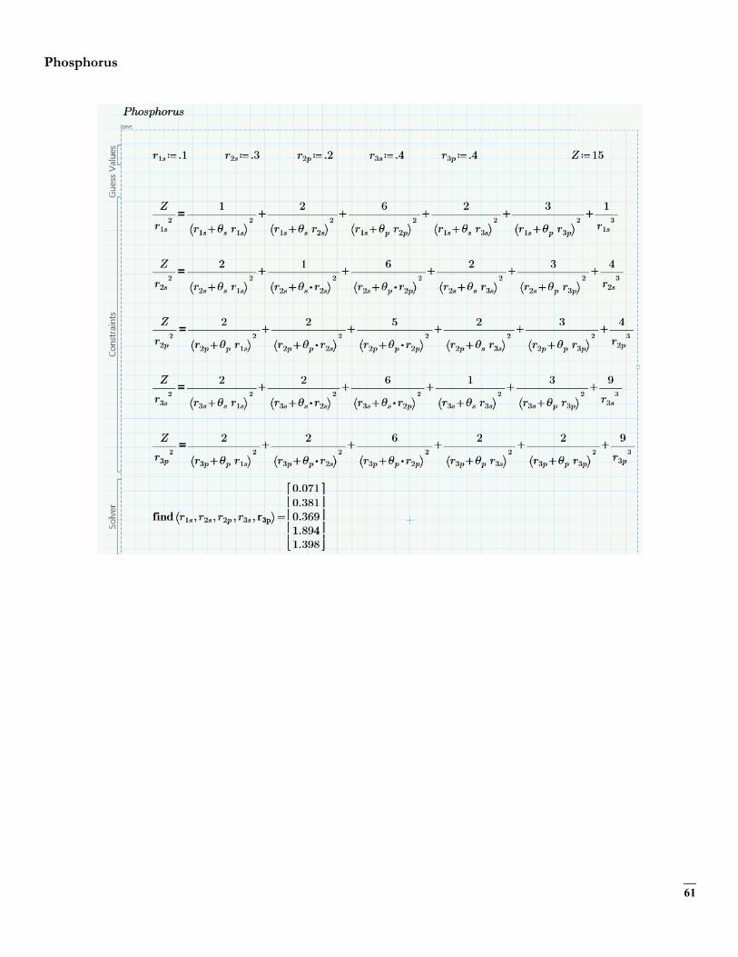
61
Phosphorus

62
Sulfur
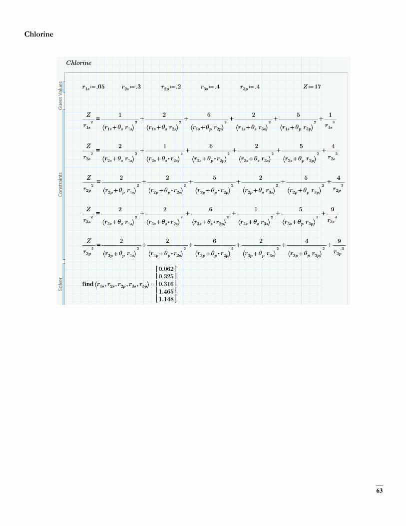
63
Chlorine
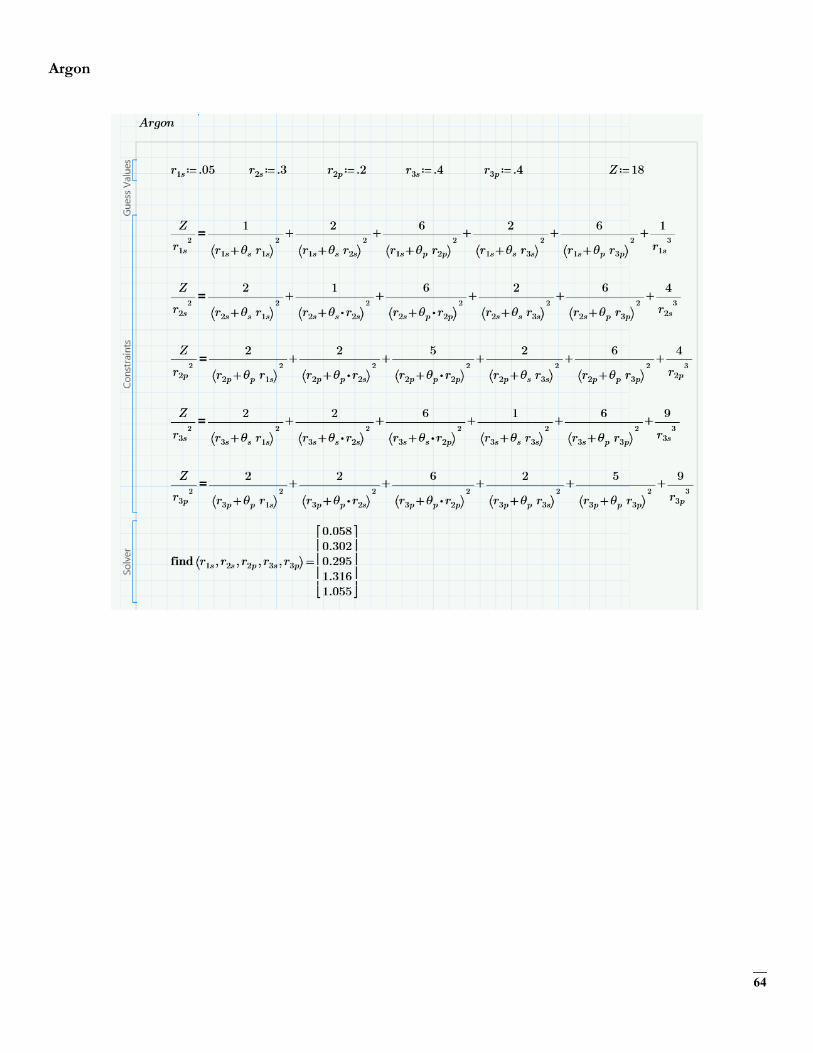
64
Argon
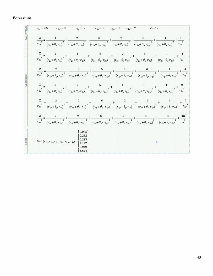
65
Potassium
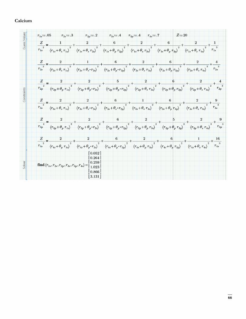
66
Calcium
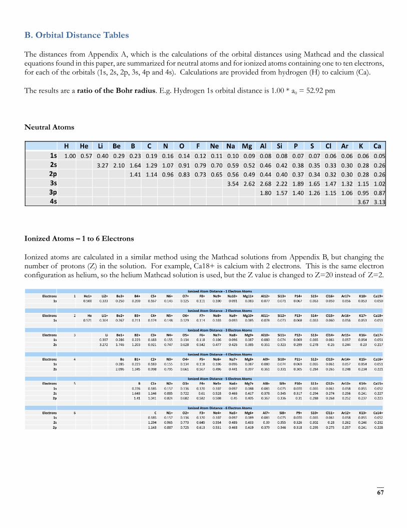
67
B. Orbital Distance Tables
The distances from Appendix A, which is the calculations of the orbital distances using Mathcad and the classical equations found in this paper, are summarized for neutral atoms and for ionized atoms containing one to ten electrons, for each of the orbitals (1s, 2s, 2p, 3s, 4p and 4s). Calculations are provided from hydrogen (H) to calcium (Ca).
The results are a ratio of the Bohr radius. E.g. Hydrogen 1s orbital distance is 1.00 * a0 = 52.92 pm
Neutral Atoms
Ionized Atoms – 1 to 6 Electrons
Ionized atoms are calculated in a similar method using the Mathcad solutions from Appendix B, but changing the number of protons (Z) in the solution. For example, Ca18+ is calcium with 2 electrons. This is the same electron configuration as helium, so the helium Mathcad solution is used, but the Z value is changed to Z=20 instead of Z=2.
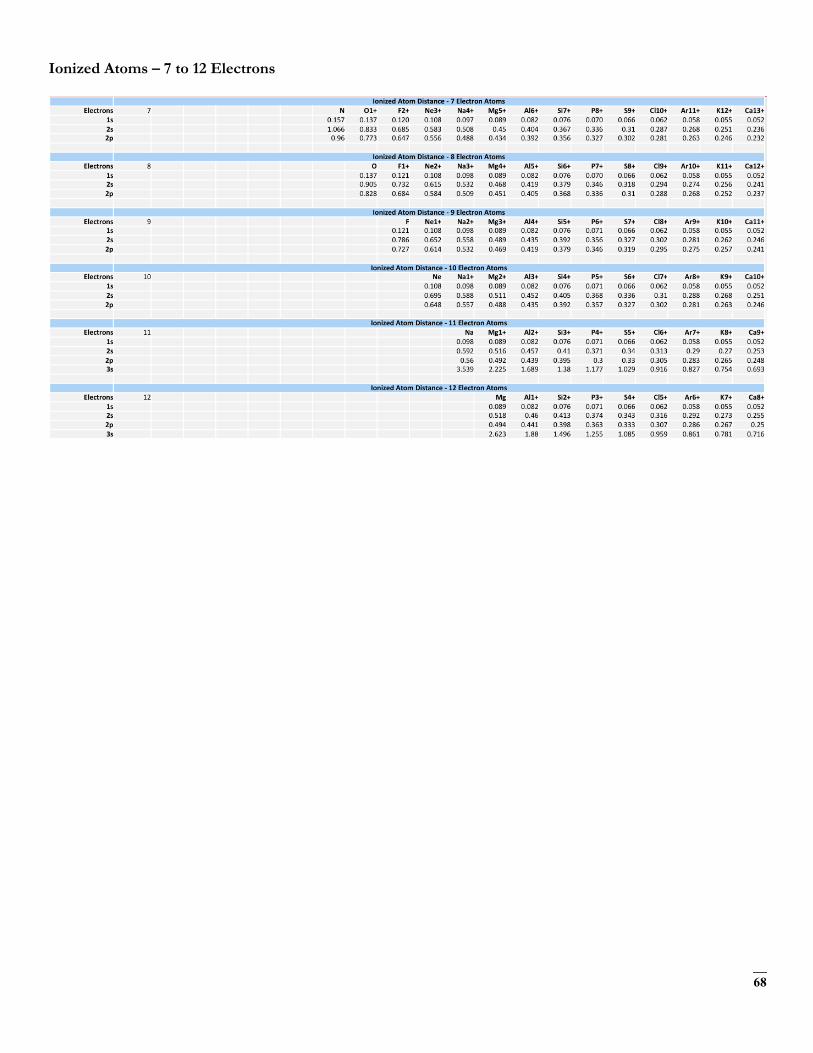
68
Ionized Atoms – 7 to 12 Electrons
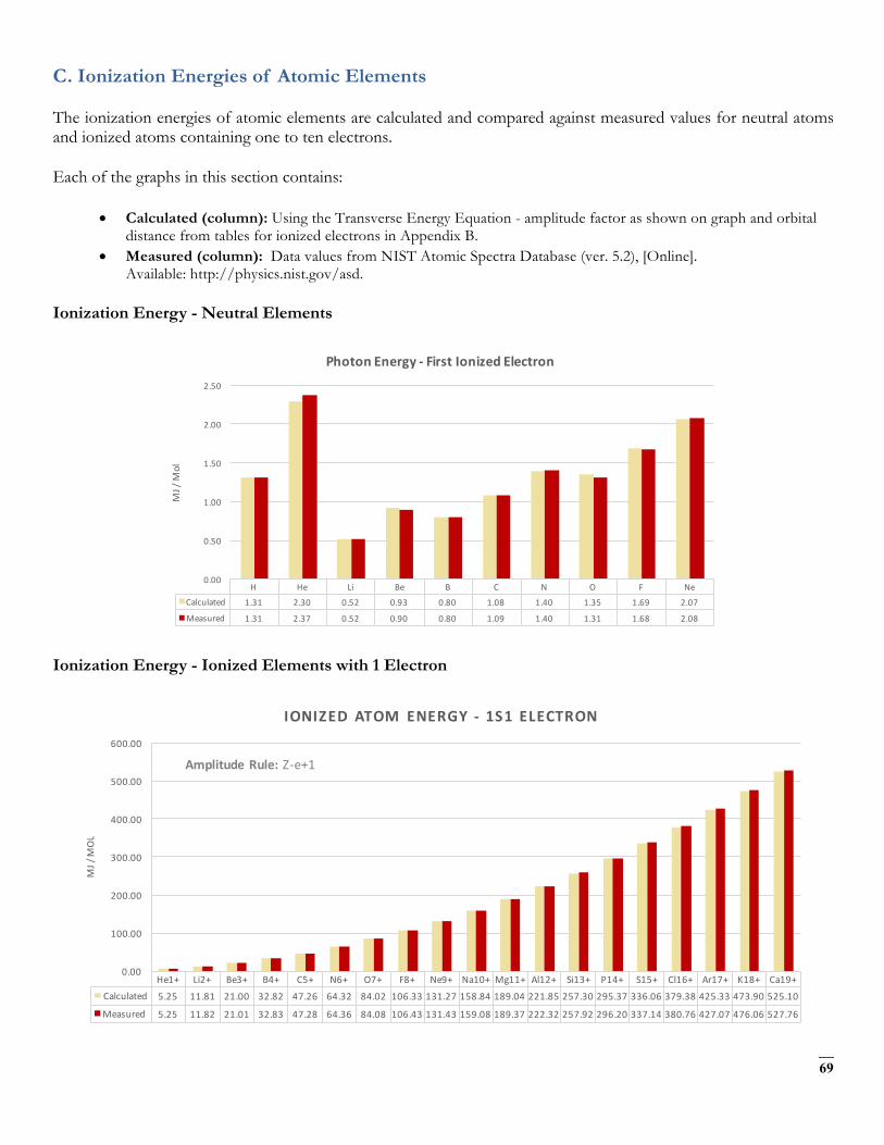
69
C. Ionization Energies of Atomic Elements
The ionization energies of atomic elements are calculated and compared against measured values for neutral atoms and ionized atoms containing one to ten electrons.
Each of the graphs in this section contains:
• Calculated (column): Using the Transverse Energy Equation - amplitude factor as shown on graph and orbital distance from tables for ionized electrons in Appendix B.
• Measured (column): Data values from NIST Atomic Spectra Database (ver. 5.2), [Online]. Available: http://physics.nist.gov/asd.
Ionization Energy - Neutral Elements
Ionization Energy - Ionized Elements with 1 Electron
H He Li Be B C N O F Ne
Calculated 1.31 2.30 0.52 0.93 0.80 1.08 1.40 1.35 1.69 2.07
Measured 1.31 2.37 0.52 0.90 0.80 1.09 1.40 1.31 1.68 2.08
0.00
0.50
1.00
1.50
2.00
2.50
MJ/M
ol
PhotonEnergy- FirstIonizedElectron
Calculated:UsingtheTransverseEnergyEquationMeasured: DatavaluesfromNISTAtomicSpectraDatabase (ver. 5.2),[Online].Available: http://physics.nist.gov/asd.
He1+ Li2+ Be3+ B4+ C5+ N6+ O7+ F8+ Ne9+ Na10+ Mg11+ Al12+ Si13+ P14+ S15+ Cl16+ Ar17+ K18+ Ca19+
Calculated 5.25 11.81 21.00 32.82 47.26 64.32 84.02 106.33 131.27 158.84 189.04 221.85 257.30 295.37 336.06 379.38 425.33 473.90 525.10
Measured 5.25 11.82 21.01 32.83 47.28 64.36 84.08 106.43 131.43 159.08 189.37 222.32 257.92 296.20 337.14 380.76 427.07 476.06 527.76
0.00
100.00
200.00
300.00
400.00
500.00
600.00
MJ/MOL
IONIZEDATOM ENERGY - 1S1 ELECTRON
AmplitudeRule: Z-e+1
Calculated:UsingTransverseEnergyEquation
Measured: DatavaluesfromNISTAtomicSpectraDatabase (ver. 5.2),[Online].Available: http://physics.nist.gov/asd.
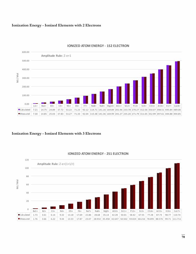
70
Ionization Energy - Ionized Elements with 2 Electrons
Ionization Energy - Ionized Elements with 3 Electrons
Li1+ Be2+ B3+ C4+ N5+ O6+ F7+ Ne8+ Na9+ Mg10+ Al11+ Si12+ P13+ S14+ Cl15+ Ar16+ K17+ Ca18+
Calculated 7.21 14.75 24.89 37.72 53.22 71.23 92.12 114.71 141.16 169.89 201.96 233.78 270.27 312.56 350.07 398.51 445.84 489.06
Measured 7.30 14.85 25.03 37.83 53.27 71.33 92.04 115.38 141.36 169.99 201.27 235.20 271.79 311.05 352.99 397.61 444.88 494.85
0.00
100.00
200.00
300.00
400.00
500.00
600.00
MJ/M
ol
IONIZEDATOMENERGY- 1S2ELECTRON
AmplitudeRule: Z-e+1
Calculated:UsingTransverseEnergyEquation
Measured: DatavaluesfromNISTAtomicSpectraDatabase (ver. 5.2),[Online].Available: http://physics.nist.gov/asd.
Be1+ B2+ C3+ N4+ O5+ F6+ Ne7+ Na8+ Mg9+ Al10+ Si11+ P12+ S13+ Cl14+ Ar15+ K16+ Ca17+Calculated 1.73 3.61 6.14 9.32 13.18 17.69 22.86 28.68 35.14 42.28 50.01 58.42 67.55 77.28 87.73 98.77 110.74
Measured 1.76 3.66 6.22 9.44 13.33 17.87 23.07 28.932 35.458 42.647 50.502 59.024 68.216 78.095 88.576 99.71 111.711
0
20
40
60
80
100
120
MJ/M
ol
IONIZEDATOMENERGY- 2S1ELECTRON
AmplitudeRule: Z-e+(1+1/r)
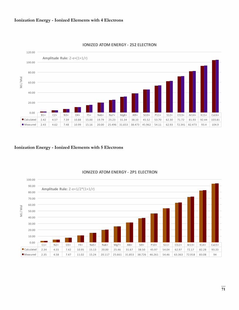
71
Ionization Energy - Ionized Elements with 4 Electrons
Ionization Energy - Ionized Elements with 5 Electrons
B1+ C2+ N3+ O4+ F5+ Ne6+ Na7+ Mg8+ Al9+ Si10+ P11+ S12+ Cl13+ Ar14+ K15+ Ca16+Calculated 2.42 4.57 7.39 10.88 15.00 19.79 25.23 31.34 38.10 45.52 53.70 62.30 71.72 81.93 92.44 103.81
Measured 2.43 4.62 7.48 10.99 15.16 20.00 25.496 31.653 38.473 45.962 54.11 62.93 72.341 82.473 93.4 104.9
0.00
20.00
40.00
60.00
80.00
100.00
120.00
MJ/M
ol
IONIZEDATOMENERGY- 2S2ELECTRON
AmplitudeRule: Z-e+(1+1/r)
C1+ N2+ O3+ F4+ Ne5+ Na6+ Mg7+ Al8+ Si9+ P10+ S11+ Cl12+ Ar13+ K14+ Ca15+Calculated 2.34 4.55 7.42 10.95 15.13 20.00 25.46 31.67 38.50 45.97 54.04 62.97 72.17 82.28 93.33
Measured 2.35 4.58 7.47 11.02 15.24 20.117 25.661 31.853 38.726 46.261 54.46 63.363 72.918 83.08 94
0.00
10.00
20.00
30.00
40.00
50.00
60.00
70.00
80.00
90.00
100.00
MJ/M
ol
IONIZEDATOMENERGY- 2P1ELECTRON
AmplitudeRule: Z-e+1/2*(1+1/r)
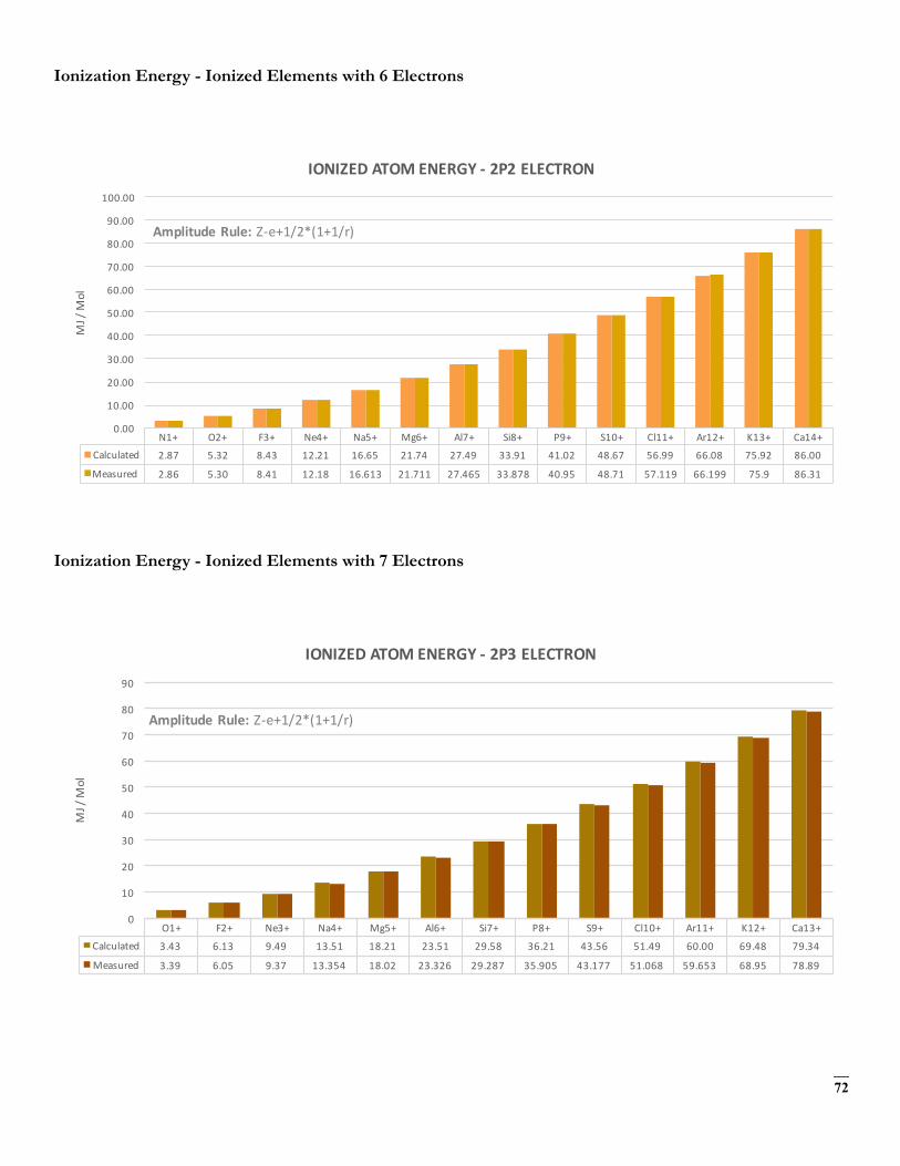
72
Ionization Energy - Ionized Elements with 6 Electrons
Ionization Energy - Ionized Elements with 7 Electrons
N1+ O2+ F3+ Ne4+ Na5+ Mg6+ Al7+ Si8+ P9+ S10+ Cl11+ Ar12+ K13+ Ca14+Calculated 2.87 5.32 8.43 12.21 16.65 21.74 27.49 33.91 41.02 48.67 56.99 66.08 75.92 86.00
Measured 2.86 5.30 8.41 12.18 16.613 21.711 27.465 33.878 40.95 48.71 57.119 66.199 75.9 86.31
0.00
10.00
20.00
30.00
40.00
50.00
60.00
70.00
80.00
90.00
100.00
MJ/M
ol
IONIZEDATOMENERGY- 2P2ELECTRON
AmplitudeRule: Z-e+1/2*(1+1/r)
O1+ F2+ Ne3+ Na4+ Mg5+ Al6+ Si7+ P8+ S9+ Cl10+ Ar11+ K12+ Ca13+Calculated 3.43 6.13 9.49 13.51 18.21 23.51 29.58 36.21 43.56 51.49 60.00 69.48 79.34
Measured 3.39 6.05 9.37 13.354 18.02 23.326 29.287 35.905 43.177 51.068 59.653 68.95 78.89
0
10
20
30
40
50
60
70
80
90
MJ/M
ol
IONIZEDATOMENERGY- 2P3ELECTRON
AmplitudeRule: Z-e+1/2*(1+1/r)
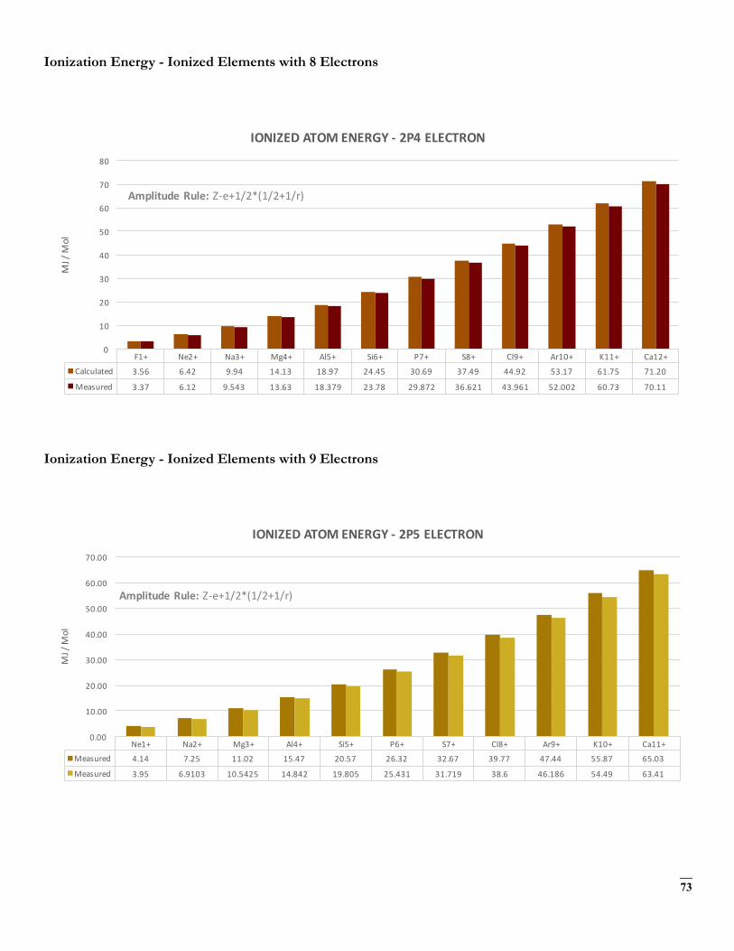
73
Ionization Energy - Ionized Elements with 8 Electrons
Ionization Energy - Ionized Elements with 9 Electrons
F1+ Ne2+ Na3+ Mg4+ Al5+ Si6+ P7+ S8+ Cl9+ Ar10+ K11+ Ca12+Calculated 3.56 6.42 9.94 14.13 18.97 24.45 30.69 37.49 44.92 53.17 61.75 71.20
Measured 3.37 6.12 9.543 13.63 18.379 23.78 29.872 36.621 43.961 52.002 60.73 70.11
0
10
20
30
40
50
60
70
80
MJ/M
ol
IONIZEDATOMENERGY- 2P4ELECTRON
AmplitudeRule: Z-e+1/2*(1/2+1/r)
Ne1+ Na2+ Mg3+ Al4+ Si5+ P6+ S7+ Cl8+ Ar9+ K10+ Ca11+Measured 4.14 7.25 11.02 15.47 20.57 26.32 32.67 39.77 47.44 55.87 65.03
Measured 3.95 6.9103 10.5425 14.842 19.805 25.431 31.719 38.6 46.186 54.49 63.41
0.00
10.00
20.00
30.00
40.00
50.00
60.00
70.00
MJ/M
ol
IONIZEDATOMENERGY- 2P5ELECTRON
AmplitudeRule: Z-e+1/2*(1/2+1/r)

74
Ionization Energy - Ionized Elements with 10 Electrons
The 2p6 configuration is the last atomic element configuration calculated using the estimation method because the accuracy begins to decline.
1 Bohr, N., On the Constitution of Atoms and Molecules - Part II Systems Containing Only a Single Nucleus, Philosophical Magazine 26, 153, (1913). 2 Liboff, R., Introductory Quantum Mechanics, (Addison-Wesley, Reading, 2002).
3 Webelements, Orbital Distances, [Online]. Available: https://www.webelements.com
4 Data values from NIST Atomic Spectra Database (ver. 5.2), [Online]. Available: http://physics.nist.gov/asd
5 Yee, J., Particle Energy and Interaction, Vixra.org 1408.0224 (2017).
6 Yee, J., Forces, Vixra.org 1606.0112 (2017).
7 Yee, J., Fundamental Physical Constants, Vixra.org 1606.0113 (2017).
8 Yee, J., Fundamental Physical Constants, Vixra.org 1705.0101 (2017).
9 NIST, CODATA Value of Bohr Radius, [Online]. Available: https://physics.nist.gov/cgi-bin/cuu/Value?bohrrada0
Na1+ Mg2+ Al3+ Si4+ P5+ S6+ Cl7+ Ar8+ K9+ Ca10+Calculated 4.76 8.13 12.14 16.82 22.14 28.19 34.87 42.15 50.02 58.82
Measured 4.562 7.7327 11.577 16.091 21.267 27.107 33.604 40.76 48.61 57.11
0
10
20
30
40
50
60
70
MJ/M
ol
IONIZEDATOMENERGY- 2P6ELECTRON
AmplitudeRule: Z-e+1/2*(1/2+1/r)

75
10 Mohr, P., Newell, D. and Taylor, B., CODATA Recommended Values of the Fundamental Physical Constants 2014 Rev. Mod. Phys. 88, 035009 (2016).
11 Zeeman, P., On the influence of Magnetism on the Nature of the Light emitted by a Substance, Phil. Mag. 43: 226 (1897). 12 Webelements, Helium Orbital Distance, [Online]. Available: https://www.webelements.com/helium/atom_sizes.html
13 Data values from NIST Atomic Spectra Database (ver. 5.2), [Online]. Available: http://physics.nist.gov/asd.
14 University of Arizona, Photoelectron Spectroscopy, [Online]. Available: http://cbc.arizona.edu/chemt/Flash/photoelectron.html
15 Science Fridays, [Online]. Image Source: https://awo.aws.org/2013/04/a-tale-of-two-models/
16 Jolly, W. L., Modern Inorganic Chemistry, (McGraw-Hill, New York,1984). 17 Chemistry Libretexts, Atomic Orbital Shapes, [Online]. Available: https://chem.libretexts.org/Core/Physical_and_Theoretical_Chemistry/Quantum_Mechanics/09._The_Hydrogen_Atom/Atomic_Theory/Electrons_in_Atoms/Electronic_Orbitals
18 IUPAC, Periodic Table of Elements, [Online]. Available: https://iupac.org/what-we-do/periodic-table-of-elements/
19 Angelo.edu, Atomic Masses (of argon and calcium), [Online]. Available: https://www.angelo.edu/faculty/kboudrea/periodic/structure_mass.htm