atmospheric turbulence-induced signal fades on optical heterodyne

Atmospheric turbulence-induced signal fades on opticalheterodyne communication links

Kim A. Winick

The three basic atmospheric propagation effects, absorption, scattering, and turbulence, are reviewed. Asimulation approach is then developed to determine signal fade probability distributions on heterodyne-detected satellite links which operate through naturally occurring atmospheric turbulence. The calculationsare performed on both angle-tracked and nonangle-tracked downlinks, and on uplinks, with and withoutadaptive optics. Turbulence-induced degradations in communication performance are determined usingsignal fade probability distributions, and it is shown that the average signal fade can be a poor measure of theperformance degradation.

1. Introduction

The Massachusetts Institute of Technology LincolnLaboratory is currently involved in the development ofheterodyne detection technology for use on high datarate, intersatellite, optical communication links. Aspart of this endeavor, we are designing a semiconduc-tor laser transmitter payload to be placed in geosyn-chronous orbit late in 1989. To lessen the cost andcomplexity of our initial technology demonstration,the companion heterodyne receiver will be located onearth, with future systems to be entirely space-based.

Atmospheric effects and the resulting degradationin system performance are major considerations in thedesign of the satellite-to-earth optical communicationlink. Atmospheric effects at optical and near-opticalwavelengths can be divided into three categories: ab-sorption, scattering, and turbulence.' Absorption andscattering primarily reduce the amplitude of the re-ceived wave front, while turbulence introduces ran-dom wave front fluctuations in both amplitude andphase. Reductions in amplitude, due to absorptionand scattering, are relatively time-invariant, changingslowly as weather conditions evolve or as clouds passoverhead. They are also nonstatistical in nature. Bycontrast, turbulence-induced fluctuations are stochas-tic and can vary at rates as high as a hundred times persecond. Although the three atmospheric effects differconsiderably, their end result is the same, namely, adegradation in communication link performance.

The author is with MIT Lincoln Laboratory, P.O. Box 73, Lexing-ton, Massachusetts 02173.

Received 5 September 1985.0003-6935/86/111817-09$02.00/0.© 1986 Optical Society of America.

This degradation is usually characterized as a loss in.signal-to-noise ratio.

The portion of this loss attributable to turbulence isstochastic and consequently can only be completelydescribed by its cumulative probability distribution.Most researchers, however, have computed only themean or variance of the loss,2 3 even though these sta-tistics alone are inadequate for predicting communica-tion system performance. A notable exception can befound in the work of Churnside and McIntyre whoused an approximate analysis involving Zernike poly-nomials to derive probability densities.4 5 Their tech-nique, however, relies on the implicit assumption thatthe coefficients in the Zernike polynomial expansionsare uncorrelated, and they are not.6 In this paper adifferent approach for calculating the probability den-sity for an optical heterodyne detection system is de-scribed. The approach is based on simulation andyields mean and variance values consistent with thoseobtained using other techniques. The method is illus-trated by evaluating the degradation in communica-tion performance on satellite-to-earth and earth-to-satellite links. The calculations are performed fordownlinks, with and without angle tracking, and foruplinks, with and without adaptive optics. Hetero-dyne detection is assumed on all links, and an operat-ing wavelength of 0.84 um is used in the calculations.7

This paper is organized as follows. Section II sum-marizes absorption and scattering effects, informationwhich should prove useful in assessing the relativeimportance of these phenomena compared with thoseof turbulence. Section III describes turbulence and itseffect on optical heterodyne detection. This discus-sion closely parallels the work of Fried.2 Section IVpresents a simulation technique for calculating signal-to-noise ratio probability densities in optical hetero-dyne detection systems. Section V specifies the near-

1 June 1986 / Vol. 25, No. 11 / APPLIED OPTICS 1817

field phase structure function, a quantity which isneeded to perform the simulations described in Sec.IV. The phase structure function is presented for fourcases: downlink, downlink with angle tracking,uplink, and uplink with adaptive optics. Section VIcontains simulation results for an optical heterodynedetection communication system. Cumulative proba-bility distributions of the received signal-to-noise ratioare given, and the resulting degradation in communi-cation system performance is quantified. Section VIIcontains our conclusions.

II. Absorption and Scattering

Absorption occurs when the optical electromagneticfield transfers energy to the molecular constituents ofthe atmosphere.89 This transfer, which can be de-scribed quantum mechanically, results in an increaseof the molecules rotational, vibrational, or electronicinternal energy. Absorption effects exhibit extremewavelength dependencies, and in some instances canbe mitigated by judiciously choosing the operatingwavelength. Figures 1 and 2 show the energy loss dueto absorption of an optical beam propagating throughthe atmosphere from a satellite to a ground station.The ground station is at an altitude of 10,000 ft-abovesea level in a tropical environment, and the zenithangle of the satellite is 450. As Figs. 1 and 2 indicate,absorption losses of <2.4 dB are to be expected be-tween 0.8380 and 0.8500 .um. Clearly, operation be-tween 0.8200 and 0.8380 ,m is ill-advised because ofthe large number of strong absorption lines which oc-cur in this band. The values given in Figs. 1 and 2 wereproduced using the HITRAN software developed at theU.S. Air Force Geophysical Laboratory.' 0

Absorption values are a function of climatologicalconditions, and thus the data presented in Figs. 1 and 2are only characteristic of a typical tropical environ-ment without cloud cover. Although absorption val-ues change with climatological conditions, the wave-length locations of the discrete absorption lines do not.In the wavelength region between 0.8 and 0.9,4m, most

z0(A

C4I-

absorption is due to atmospheric water vapor content.Scattering, as opposed to absorption, does not pro-

duce a net change in the internal energy states ofmolecules. It is explained in terms of electromagneticwave theory and the electron theory of matter.' Scat-tering occurs when the optical electromagnetic wavesets in oscillation the electric charges which constitutethe scattering particle. This particle can be any bit ofmatter such as an air molecule or a fog droplet. Scat-tering losses are not a strong function of wavelength atvisible and near visible wavelengths. They are, how-ever, a strong function of visibility conditions. At awavelength of 0.84 jim, a computer code produced bythe U.S. Air Force Geophysics Laboratory' 2 indicatesthat a scattering loss of <1 dB is to be expected on asatellite-to-earth communication link. This 1-dB val-ue assumes that the ground station is at an altitude of10,000-ft above sea level, the satellite zenith angle is450, weather conditions at sea level are clear (i.e., visi-bility = 20 km), and there is no cloud cover. Opticalscattering losses due to even small amounts of cloudcover can be severe (i.e., greater than tens of decibels),thus limiting communications to those time periodswhen there are no clouds.

Ill. Turbulence and Optical Heterodyne Detection

Turbulence refers to the time-varying inhomogen-eous refractive-index structure of the atmosphere, andit is even present in excellent visibility conditions.The refractive-index inhomogeneity is of the order ofone part in a million and is a result of the nonuniformtemperature structure of the atmosphere. Turbu-lence can be modeled qualitatively as if the atmo-sphere consisted of a set of seak lenses of varyingdiameters. The atmosphere changes in time as theselenses are moved by the winds. A stationary lenswhich is larger than the beam diameter will onlychange the angular orientation (i.e., tilt) of the propa-gating beam. Thus, the wind-induced motion of largelenses will cause the beam to dance around its nominalarrival angle. Conversely, lenses which are small with

z0InCD

I-

WAVELENGTH (Mm)

Fig. 1. Absorption spectral line plot (0.82-0.84 im).

0.840 0.845WAVELENGTH (gm)

0.860

Fig. 2. Absorption spectral line plot (0.84-0.85 gm).

1818 APPLIED OPTICS / Vol. 25, No. 11 / 1 June 1986

Iu

0.7

).5

).4

0.3

).2

)0 .

r I I , I I I I I I'

I

I

I

l

LOAD

Fig. 3. Optical heterodyne receiver structure.

respect to the beam diameter lead to diffraction ef-fects, and these diffractive effects result in beambroadening and intensity scintillation. The nature ofturbulence differs from both absorption and scatteringbecause it has a relatively rapid time-varying charac-teristic (i.e., up to -100 Hz) and because it distorts thephase, not just the amplitude, of the received wavefront. It is this turbulence-induced phase perturba-tion which limits the resolution of the best ground-based telescopes, regardless of size, to -1 sec of arc.13"14

Figure 3 illustrates the optical heterodyne receiverstructure associated with a communication link from asatellite to a ground station. The receiver structureshown has been simplified for the sake of clarity, andthe discussion which follows parallels the work ofFried.2 The effect of atmospheric turbulence can bemodeled as an amplitude and phase perturbation ofthe received beam. These perturbations are ex-pressed mathematically by writing the received signalfield, Es(X), as follows:

E,(X) = As(X) exp[io(X)] exp(i2irfst), (1)

where A,(X), 0(X), and fs are the amplitude, phase,and frequency of the field at point X. We treat thecase of frequency modulation for which the signal in-formation is contained inf,. If the modulation is 8-aryfrequency shift keying (FSK), As can assume one ofeight discrete frequencies. In the absence of turbu-lence AS(X) and 0(X) are constants.

As indicated in Fig. 3, the received signal field ismixed with a plane wave local oscillator field, EJ(X),described by

E0 (X) = A, exp(ip1) exp(i2irfot). (2)

The current I produced by the photodetector is pro-portional to the power of the incident field integratedover the detector's collection aperture. Thus we canwrite

I = X S W(X)[E(X) + EJ(X)][E0(X) + E,(X)I*dX, (3)

where x1 = detector quantum efficiency,

1,I -I'W(X) = (4)

and * denotes complex conjugate. Note that W(X)

defines the region of the detector's collection aper-ture-assumed to be a circle of diameter d. Combin-ing Eqs. (1)-(3) yields

I = X S W(X)A 2(X)dX + X f W(X)A2dX

+ 7 S W(X)2A.A8(X) cos[2r(f, - fo)t + 0(X) - o]dX. (5)

Since in a well-designed heterodyne detection systemthe local oscillator power is considerably larger thanthe received signal power,'5 Eq. (5) can be written as

I- f W(X)A'dX + n f W(X)2A0A,(X)X cos[2ir(fs - fo)t + O(X) - 4O]dX. (6)

The information containing portion of the photocur-rent, denoted I, is clearly given by

I = X f W(X)2AA,(X) cos[2r(f - f)t + d(X) - koJdX. (7)

Thus the information bearing signal power received bythe demodulator, P8, is given by

Ps = ((GIs)2 R) = 4G2R,72A'({fW(X)A,(X)

X cos[2r(fs - f)t + ¢P(X) -4 00]dX12), (8)

where the brackets ( ) denote a time average. Equa-tion (8) can be written as

P = 2G2RiA 2 ff W(X) W(X')A8 (X)A,(X')

X (cos[4ir(f, - fo)t + (X) + (X') - 2 6])dXdX'

+ 2G2R 2 A2 55 W(X)W(X')A0 (X)A,(X')

x cos[O(X) - (X')]dXdX'- 2G2 Rn2 A2 55 W(X) W(X')A 0 (X)A,(X')

X cos[O(X) - (X')]dXdX'. (9)

In the last step above, the term containing cos[4,r(f, -fo)t + q5(X) + 0(X') - 2] has been dropped, because itoscillates so rapidly that its time average is zero. Us-ing complex notation, Eq. (9) becomes

P = 2G2 R, 2A 2 1 W(X)As(X) exp[i0(X)]dXI 2 . (10)

If loss v is defined as the signal power in the presence ofturbulence divided by the signal power in the absenceof turbulence, it follows from Eq. (10) that

lo IS W(X)A,(X) exp[i1(X)]dXi 2

A2(f W(X)dX) 2 (11)

where

As(X) = constant = A in the absence of turbulence. (12)

Note that the loss in signal-to-noise ratio equals theloss in signal power.

The mean and variance of v have been calculatedanalytically by Fried,23 but there is an error in hisvariance calculation.'6 The error stems from an ap-proximation made in Sec. III of his paper. Banakh16and Massa17 have performed variance calculations us-ing a Monte Carlo numerical integration techniquewhich avoids Fried's error. It is our goal, however, asstated in Sec. I, to compute the cumulative probabilitydistribution of v rather than only its first and secondmoments.

We note that most of the atmospheric turbulenceoccurs within the first 10 km of the earth's surface.


Thus, for a reasonably sized earth-based collectionaperture (i.e., d > 10 cm) and for a wavelength of 0.84gida, the turbulence is within the near field [i.e., d > (104X 0.84 X 10-6)1/2 m].

In such a situation, it can be shown that most of theloss in signal-to-noise ratio is due to the phase pertur-bhtion (X) rather than the amplitude scintillationA,(X).18 Thus, we can write

v w f W(X) exp[i41(X)]dXI2 (13)

where

X = ( W(X)dX) 2 = (area of collection aperture) 2 . (14)

It is not necessary to neglect amplitude scintillation inorder to use the simulation technique described in thenext section, but it does simplify matters greatly.

IV. Probability Density Calculation

It was shown in the previous section that the loss insignal-to-noise ratio v is given by

v Al, WIf WM exp[i0(X)jdN2, (15)

where

,> = [S W(X)dX] 2 (16)

In this section, a simulation technique for calculatingthe probability distribution of v will be described.

Equation (15) can be written as follows:

v w an1 If W(X) exp[i0(X)]dXI 2 (17)

where

O(X) A (X) -0(0). (18)

The phase 0(X) of the received wave front is a statisti-cal quantity which is both Gaussian and stationary inX.' 9 Thus the quantity (X) is a zero mean, station-ary, Gaussian random process, and as such is complete-ly specified by its autocorrelation function R0(X - X')defined by

R,(X - X') A 8(X)O(X'), (19)

where the overbar denotes a statistical average.Using the algebraic identity

(a - b)(c - d) = -/ 2(a - c)2 - /2(b -d)2

+ /2(a - d)2 + 1/2(b - )2 , (20)

it follows that

Ro(X - X') = - [0(X) - 4(X')]2 + [1(X) - 0(0)]22 ~~~~2

+ 1 [05(X') - 4(o)]2

= D-D(X - X') + 2 D(X') + D(X), (21)

~Where

DO(a) A [(X + 6) -0(X)]2 . (22)

D4,(6), which is referred to as the phase structure func-tion in atmospheric optics, will be specified in Sec. V.

For now, however, let us assume that D 1(6) and henceR¢,(X - X') are known.

The integral in Eq. (15) can be approximated by thefollowing sum:

1 N 2

V Z_ _ exp[iO(Xj)] Ii=1

(23)

where the X,X 2, .. ., XN are N sample points withinthe collection aperture. In Appendix A it is shownthat the mean-squared error E that results from ap-proximating the integral of Eq. (17) by this sum isbounded above by

e < 4- f W(X) W(Y) exp [- D(X - Y)] dXdY

-81-/2 1 EJ exp [-2 D(X -Xj)] dX

+ 4 2 E E exp [-2 DO(X - XK)1.j=1 K=1J

(24)

Note that the O(X), . . . , O(XN) are zero mean, identi-cally distributed, correlated Gaussian random vari-ables. A method for evaluating v using a computerexperiment now becomes apparent. Statistically in-dependent sets of O(X), . . . , O(XN) are generated Mtimes, and for each of these sets v is computed usingEq. (23). The cumulative probability distribution,Pcun(Z), defined by

(25)pCm(Z) A probability v < z,

is then approximated as follows:

Pcum(Z) (number of times v < z)M

The variance of the estimate of Pcum(z) is the varianceof a binomial distribution. Thus,

variance = Pcum(z) [1 - Pcum(Z)]/M (27)

A technique for generating the correlated Gaussianrandom variables, 0(X), . ., O(XN), is described next.

There are simple methods available for generatingstatistically independent Gaussian random vari-ables.20 Let G denote an N X 1 column vector consist-ing of N, zero mean, unit variance, statistically inde-pendent, Gaussian random variables generated by oneof these methods. Then we will show that there existsa matrix C such that the matrix product C * G is an N X1 column vector whose elements are 0(X), . , (XN) -We note that this method of generating correlatedGaussian random variables is essentially the inverse ofthe whitening process commonly encountered in sta-tistical communication theory.2'

Let B denote the N X N correlation matrix whosejth, kth element bk (i.e., the element in row j andcolumn k) is defined as

bjkA O(Xj)O(Xk) R(Xj - Xk). (28)

Note that the elements of the column vector C G areGaussian, because linear transformations preserveGaussian statistics.22 It is also clear that the elements


(26)

of C G are zero mean. Thus, it is sufficient to find amatrix C which satisfies the following condition:

B = (C G)(C G)t , (29)

where superscript t denotes the matrix transpose. Wealso note that

(C G *(C G)t = C G . Gt. Ct = C . Ct. (30)

Since B is a correlation matrix it must be real, sym-metric, and positive semidefinite.23 From the real andsymmetric property it follows that B has a complete setof N orthonormal eigenvectors, and from the positivesemidefinite property it follows that the correspondingeigenvalues must be non-negative.24 Let T denote thematrix whose columns Tj are the orthonormal eigen-vectors of matrix B. Let X denote the eigenvaluecorresponding to the eigenvector T. Then we canwrite

Fig. 4. h - X coordinate system.

can be written as a function of two variables h and Xwhich together specify position. The quantities h andX are defined in Fig. 4. The statistical properties ofturbulence have been studied by Kolmogorov,25 andhis work along with others has led to the followingrelationship (Ref. 19, p. 164):

B T=T.[ 2 J.Tt1 0 X

1 0 0

B =T- x1/2 | - 12/2O 21/2 011/F

[n(h,X) - n(h',X')] 2= cn (h 2 )

*X - X12 + (h - h')2]1/3, (34)

where C2( ), the refractive-index structure parameter,is a measurable quantity which is a function of altitudeabove the earth's surface. The refractive-index struc-ture parameter changes with time of day, time of year,and with local atmospheric conditions.26 Figure 5

(1) shows two C2 profiles provided by the Rome Air Devel-opment Center, and these profiles will be used to gen-erate our results in Sec. VI.

Comparing Eqs. (29)-(31) yields the following desiredresult:

X1/2

C = T A/2 * (32)

0 XN

Thus, determining the matrix C is equivalent to find-ing the eigenvalues and eigenvectors of matrix B. Theresults of Sec. VI are based on a fifty point,X1,X2, ... ,XN, sampling of the collection aperture.The correlation matrix B is then evaluated using Eqs.(21), (22), and (28). Finally, the eigenvectors andeigenvalues of the 50 X 50 matrix B are computed usinga scientific software package.

V. Phase Structure Function

In this section the phase structure function, D,5,(),defined by Eq. (22) is specified. Four cases are consid-ered-downlink, downlink with angle tracking, uplink,and uplink with adaptive optics. D,5(5) can be calcu-lated using several different methods, all of which areperturbation techniques.'9 These techniques yieldapproximate solutions to the stochastic electromag-netic wave equation given by

VE+(2r 2f()En, 2E = , (33)

where E is the electric field vector, X is the wavelength,and n is the refractive index of the atmosphere. n is astatistical quantity, and thus Eq. (33) is stochastic. n

A. Downlink

For the downlink it was first shown by Tatarski' 9

thatD¢(B) I ([4(X + a) - 4(X)]2 ) = 2.91(sec2a)151/3

J C2(h)dh, (35)fon

where a = zenith angle of the satellite. A simple rayoptics derivation of Eq. (35) can also be found in apaper by Fried.27 In the literature, Eq. (35) is oftenwritten as

D (X -X 2) = 6.88(lX, -Xj/ro)5/3, (36)

where

rA A transverse coherence length

= [.423(sec2a) (2,r)2 f C2(h)dh]-3/5 (37)

Using Eq. (37) and the C2 profiles of Fig. 5, the daytimeand nighttime values of r (at X = 0.84 Am) are calculat-ed to be 8.9 and 16.4 cm, respectively.

B. Downlink with Angle Tracking

As discussed in Sec. III, turbulent effects can bedivided into three categories-angle of arrival fluctua-tions, beam spreading, and scintillation. A significantportion of the turbulence-induced signal loss in a het-erodyne detection system is due to angle of arrivalfluctuations alone, and this loss can be removed bytracking the arrival angle of the downlink beam. Be-cause of imperfect orbit prediction capabilities and


< SATELLITE

EARTH STATION,

EARTH

x = (x.y)

because the earth-based antenna gain pattern is ex-tremely narrow, angle tracking is probably required onthe downlink even if there is no turbulence. Thus, it isreasonable to determine communication performancein the presence of turbulence assuming downlink angletracking. The angle-tracked phase structure func-tion, D T(6), is needed to perform this task. D T(5)was first calculated (approximately) by Fried, and heobtained the following result14:

DAT(a) 6.88(QM/ro) [1 - (IS/d)13]. (38)

Fried's calculation assumed that the phase of the tiltcorrected wave front and the tilt component itself wereuncorrelated. Although this assumption is not valid,the final result expressed by Eq. (38) remains reason-ably accurate. In fact, we have evaluated the angle-tracked phase structure function exactly and havefound Eq. (38) to be in error by <6.88(8I/ro) 5 /3 1.5 X10-2.

C. Uplink

Using reciprocity arguments developed by Shapiro28

and by Fried and Yura29 for optical propagation, it canbe rigorously shown that uplink and downlink lossstatistics will be identical. In this subsection, a sim-pler, less rigorous approach is used to demonstrate thisfact.

The transmitting aperture of a geosynchronous sat-ellite is so far removed from the earth that it appears asa point source when viewed by the receiver on earth.Consequently, the downlink beam is essentially colli-mated by the time it reaches the atmosphere, anddiffraction effects arising from the finite size of thesatellite transmitting aperture can be safely neglected.On the uplink a similar situation does not exist, sincethe atmosphere lies in close proximity to the earth-based transmitter. Thus, the uplink beam will notremain collimated as it propagates through the atmo-sphere (even in the absence of turbulence) but willexperience diffraction because of the finite size of theearth-based transmitting aperture. In our analysis,these uplink diffraction effects will be neglected,which is tantamount to assuming that the atmospherelies deep in the near field of the earth-based aperture.

This assumption appears reasonable at a wavelengthof 0.84 Am, provided the diameter of the earth-basedaperture exceeds 10 cm. If necessary, the uplink dif-fraction effects discussed above can be accounted forby using extended Huygens-Fresnel diffraction tech-niques. 3 0

Since diffraction within the atmosphere is beingneglected, ray optics methods are applicable. Usingray optics, it follows that the optical field at the toplayer of the atmosphere on the uplink is identical tothat which is present at the bottom layer of the atmo-sphere on the downlink. Thus, Eq. (35) remains avalid description for the uplink phase statistics at thetop layer of the atmosphere.

It will be assumed that the distorted wave front atthe top layer of the atmosphere lies in the far field ofthe satellite receiving aperture. This is a reasonableassumption (at a wavelength of 0.84 Am) for satellitesin geosynchronous orbit. In the far field the receivedelectric field E(X') at the satellite will be proportionalto the Fourier transform of the field at the top of theatmospheres' This Fourier transform relationshipcan be written as follows:

Eu(X) W(X) exp[i(X)] exp [-i a X. X,] dX, (39)

whereW(X)= 1, inside the earth-based transmitting aperturel

to, elsewhere, JL =distance between top of atmosphere and satellite.

For satellites in geosynchronous orbit and for earth-based transmitting and satellite receiving aperture di-ameters of the order of 20 cm or less, it follows that theterm (X X')/(XL) in Eq. (39) is approximately zero.Thus Eq. (39) reduces to

(40)

The result given by Eq. (40) implies that, unlike thedownlink, the optical field received on the uplink is aplane wave.

The received signal strength on the uplink is equal toI E,(X')12. Therefore, the turbulence-induced loss onthe uplink will be given by

io1

w DA~~~~~Y10-15

I. NIGHT. 10-16

cc t

F10.17

C.,.

l 10 19 . ,,10 102 103 104 105

ALTITUDE ABOVE SITE m)

Fig. 5. Refractive-index structure function profiles.

loss = I W(X) exp[i0(X)]dX 2

If W(X)dXI2(41)

Note that Eq. (41) is identical to Eq. (13), and thus theprobability distribution of the signal-to-noise ratioloss is the same for the uplink as for the downlink.

D. Uplink with Adaptive Optics

By sensing the downlink beam from the satellite, thephase perturbation introduced by the turbulent atmo-sphere can be determined. This information can thenbe used to predistort the uplink beam (i.e., subtractfrom it the downlink phase perturbation) before trans-mission to compensate for the turbulence on the earth-to-satellite uplink. If the uplink and downlink pathswere identical, in principle total uplink compensationcould be achieved. There are two fundamental factors


E,,(X'),x f W(X) exp[i0(X)]dX.

-

SATELLITE POSITION ATTIME to

SATELLITE POSITION ATTIME t + 2At

X X

DO NLINK BEAM LEAVES w r v UPLINK BEAM LEAVES EARTH ATSATELLITE AT TIME t ARRIVE TIME t t ARRIVES AT SATELLITE

AT EARTH AT TIME t At AT TIME t + 2t

EARTH STATION POSITIONAT TIME t + At

At = SATELLITE-TO-EARTH PROPAGATION PATH LENGTH/SPEED OF LIGHTr = 2(Angular Rotation Rate of Earth)At

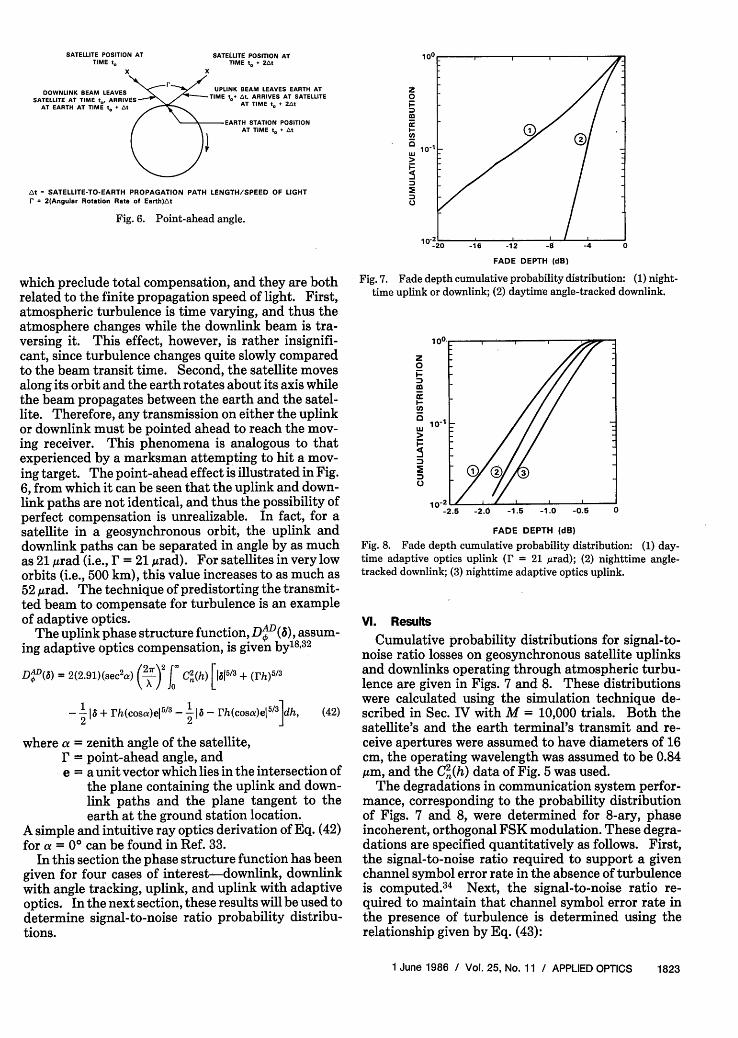
Fig. 6. Point-ahead angle.

which preclude total compensation, and they are bothrelated to the finite propagation speed of light. First,atmospheric turbulence is time varying, and thus theatmosphere changes while the downlink beam is tra-versing it. This effect, however, is rather insignifi-cant, since turbulence changes quite slowly comparedto the beam transit time. Second, the satellite movesalong its orbit and the earth rotates about its axis whilethe beam propagates between the earth and the satel-lite. Therefore, any transmission on either the uplinkor downlink must be pointed ahead to reach the mov-ing receiver. This phenomena is analogous to thatexperienced by a marksman attempting to hit a mov-ing target. The point-ahead effect is illustrated in Fig.6, from which it can be seen that the uplink and down-link paths are not identical, and thus the possibility ofperfect compensation is unrealizable. In fact, for asatellite in a geosynchronous orbit, the uplink anddownlink paths can be separated in angle by as muchas 21 grad (i.e., r = 21 girad). For satellites in very loworbits (i.e., 500 km), this value increases to as much as52,grad. The technique of predistorting the transmit-ted beam to compensate for turbulence is an exampleof adaptive optics.

The uplink phase structure function, Dy(a), assum-ing adaptive optics compensation, is given by'8 32

DAD(a) = 2(2.91)(sec2a) (2)7 J C2(h) [15l5/3 + (h) 5 /3

1 1 , I I / 3 --6 + rh(cosa)e - -rh(cosa)el5/3 dh, (42)

2 2

where a = zenith angle of the satellite,r = point-ahead angle, ande = a unit vector which lies in the intersection of

the plane containing the uplink and down-link paths and the plane tangent to theearth at the ground station location.

A simple and intuitive ray optics derivation of Eq. (42)for a = 00 can be found in Ref. 33.

In this section the phase structure function has beengiven for four cases of interest-downlink, downlinkwith angle tracking, uplink, and uplink with adaptiveoptics. In the next section, these results will be used todetermine signal-to-noise ratio probability distribu-tions.

Fig. 7. Fade depth cumulative probability distribution: (1) night-time uplink or downlink; (2) daytime angle-tracked downlink.

100-

z0

10-

LU

10-2-2.5 -2.0 -1.5 -1.0 -0.5 0

FADE DEPTH (dB)

Fig. 8. Fade depth cumulative probability distribution: (1) day-time adaptive optics uplink (r = 21 Mrad); (2) nighttime angle-tracked downlink; (3) nighttime adaptive optics uplink.

VI. Results

Cumulative probability distributions for signal-to-noise ratio losses on geosynchronous satellite uplinksand downlinks operating through atmospheric turbu-lence are given in Figs. 7 and 8. These distributionswere calculated using the simulation technique de-scribed in Sec. IV with M = 10,000 trials. Both thesatellite's and the earth terminal's transmit and re-ceive apertures were assumed to have diameters of 16cm, the operating wavelength was assumed to be 0.84gim, and the C'(h) data of Fig. 5 was used.

The degradations in communication system perfor-mance, corresponding to the probability distributionof Figs. 7 and 8, were determined for 8-ary, phaseincoherent, orthogonal FSK modulation. These degra-dations are specified quantitatively as follows. First,the signal-to-noise ratio required to support a givenchannel symbol error rate in the absence of turbulenceis computed.34 Next, the signal-to-noise ratio re-quired to maintain that channel symbol error rate inthe presence of turbulence is determined using therelationship given by Eq. (43):


z0

Mcc

I-(0Qa0

FADE DEPTH (dB)

0

Pcturb -1= IPcs (v -lp(v)dv, (43)

where S/N = signal-to-noise ratio,purb (S/N) = channel symbol error in the presence of

turbulence,PC(S/N) = channel symbol error rate in the absence

of turbulence, andp(v) = probability density of the signal-to-

noise ratio loss v due to turbulence.Finally, the degradation is computed as the differ-

ence between the above two signal-to-noise ratios. Wehave chosen to specify the degradation at an 8-arychannel symbol error rate of 1.5%. If rate 1/2, con-straint length 7, convolutional encoding is used in con-junction with 8-ary FSK modulation, the 1.5% channelsymbol error rate corresponds to approximately a 2 X10-7 hard decision, Viterbi decoded, user bit error rate.

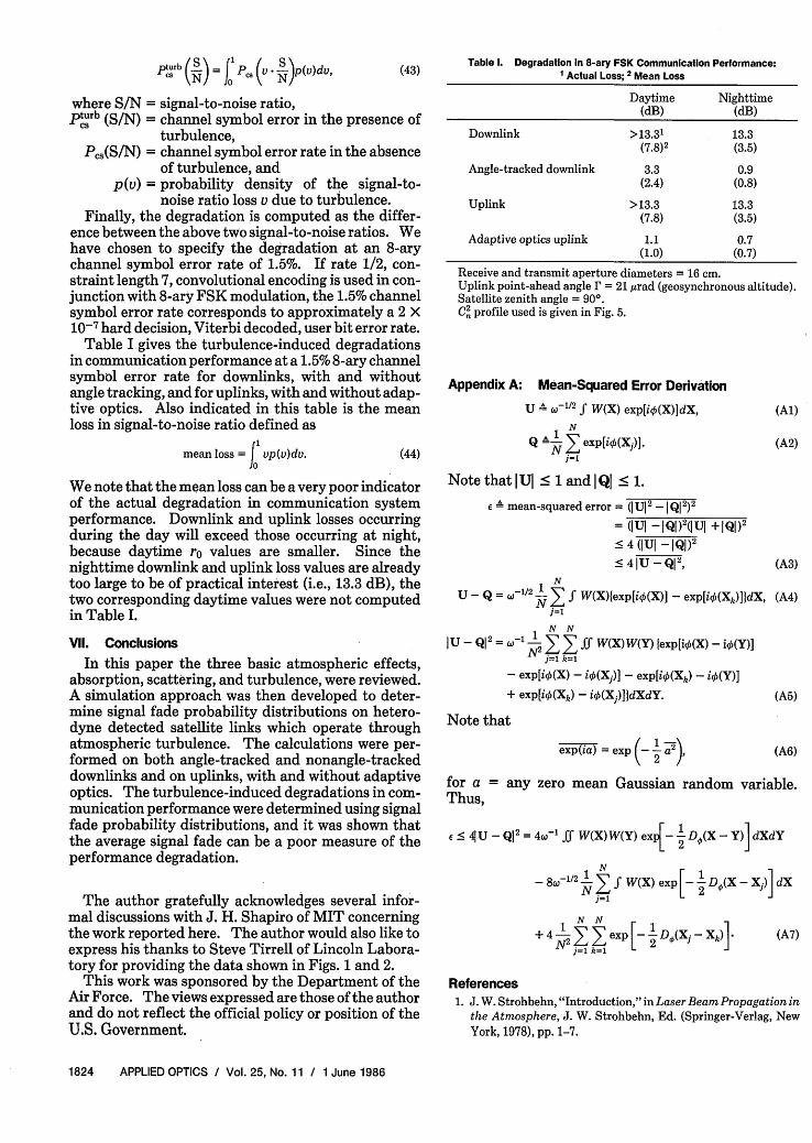
Table I gives the turbulence-induced degradationsin communication performance at a 1.5% 8-ary channelsymbol error rate for downlinks, with and withoutangle tracking, and for uplinks, with and without adap-tive optics. Also indicated in this table is the meanloss in signal-to-noise ratio defined as

mean loss = J vp(v)dv. (44)

We note that the mean loss can be a very poor indicatorof the actual degradation in communication systemperformance. Downlink and uplink losses occurringduring the day will exceed those occurring at night,because daytime r values are smaller. Since thenighttime downlink and uplink loss values are alreadytoo large to be of practical interest (i.e., 13.3 dB), thetwo corresponding daytime values were not computedin Table I.

Vil. Conclusions

In this paper the three basic atmospheric effects,absorption, scattering, and turbulence, were reviewed.A simulation approach was then developed to deter-mine signal fade probability distributions on hetero-dyne detected satellite links which operate throughatmospheric turbulence. The calculations were per-formed on both angle-tracked and nonangle-trackeddownlinks and on uplinks, with and without adaptiveoptics. The turbulence-induced degradations in com-munication performance were determined using signalfade probability distributions, and it was shown thatthe average signal fade can be a poor measure of theperformance degradation.

The author gratefully acknowledges several infor-mal discussions with J. H. Shapiro of MIT concerningthe work reported here. The author would also like toexpress his thanks to Steve Tirrell of Lincoln Labora-tory for providing the data shown in Figs. 1 and 2.

This work was sponsored by the Department of theAir Force. The views expressed are those of the authorand do not reflect the official policy or position of theU.S. Government.

Table 1. Degradation In 8-ary FSK Communication Performance:Actual Loss; 2 Mean Loss

Daytime Nighttime(dB) (dB)

Downlink >13.31 13.3(7.8)2 (3.5)

Angle-tracked downlink 3.3 0.9(2.4) (0.8)

Uplink >13.3 13.3(7.8) (3.5)

Adaptive optics uplink 1.1 0.7(1.0) (0.7)

Receive and transmit aperture diameters = 16 cm.Uplink point-ahead angle r = 21,urad (geosynchronous altitude).Satellite zenith angle = 90°.Cn profile used is given in Fig. 5.

Appendix A: Mean-Squared Error Derivation

U A W-1/2 f W(X) exp[i4(X)]dX,

N1=1

Note that Ul < 1 and I Q < 1.

e mean-squared error = (I Ul 2 - I Q 2)2

= (IUl -IQI) 2 (U +IQI) 2

< 4 (U -IQ) 2

41U -Q12,

U-Q = &'1/2 N f W(X)exp[i1(X)] - exp[i0(Xk)]1dX,j=1

N IU - Q12 = l >2 E if sW(X)W(Y) texp[i1(X) - i4(Y)]j=1 k=1

- exp[i(X) - i0(X)] - exp[io(Xk) - i(Y)]

+ exp[i(Xk) - i(X)]1dXdY.

Note that

exp(ia) = exp (- 2 2),

(Al)

(A2)

(A3)

(A4)

(A)

(A6)

for a = any zero mean Gaussian random variable.Thus,

e < U - Q12 = 4-' f W(X)W(Y) exl{- 2 DO(X - Y)] dXdY

1/2 1 1- 8w-1' N Z W(X) exp [- D0(X - X) dX

j=1

+ 4 >" E exp [- D(XJ - Xk)1j=1 k=1

(A7)

References1. J. W. Strohbehn, "Introduction," in Laser Beam Propagation in

the Atmosphere, J. W. Strohbehn, Ed. (Springer-Verlag, NewYork, 1978), pp. 1-7.


2. D. L. Fried, "Optical Heterodyne Detection of an Atmospheri-cally Distorted Signal Wave Front," Proc. IEEE 55, 57 (1967).

3. D. L. Fried, "Atmospheric Modulation Noise in an Optical Het-erodyne Receiver," IEEE J. Quantum Electron. QE-3, 213(1967).

4. J. H. Churnside and C. M. McIntyre, "Signal Current Probabili-ty Distribution for Optical Heterodyne Receivers in the Turbu-lent Atmosphere. 1: Theory," Appl. Opt. 17, 2141 (1978).

5. J. H. Churnside and C. M. McIntyre, "Signal Current Probabili-ty Distribution for Optical Heterodyne Receivers in the Turbu-lent Atmosphere. 2: Experiment," Appl. Opt. 17,2148 (1978).

6. R. J. Noll, "Zernike Polynomials and Atmospheric Turbulence,"J. Opt. Soc. Am. 66, 207 (1976).

7. J. E. Kaufmann and L. L. Jeromin, "Optical Heterodyne Inter-satellite Links Using Semiconductor Lasers," in IEEE GLOBE-COM '84, Convention Record, Atlanta, GA (26-29 Nov. 1984).

8. E. J. McCartney, Absorption and Emission by AtmosphericGases (Wiley, New York, 1983), Chap. 1.

9. R. K. Long, "Atmospheric Absorption and Laser Radiation,"Bulletin 199 (Engineering Experiment Station, Ohio State U.,Columbus, OH).

10. L. S. Rothman, "High Resolution Atmospheric TransmittanceRadiance: HITRAN and the Data Compilation," Proc. Soc. Pho-to-Opt. Instrum. Eng. 142, 2 (1978).

11. E. J. McCartney,-Optics of the Atmosphere (Wiley, New York,1976), pp. 20-26.

12. F. X. Kneizys et al.,"Atmospheric Transmittance/Radiance:Computer Code LOWTRAN 5," AFGL Report AFGL-TR-80-0067 (Air Force Geophysics Laboratory, Lexington, MA, 1980),AD No. A088215.

13. L. W. Fredrick and R. H. Baker, Astronomy (Van Nostrand,New York, 1976), p. 85.

14. D. L. Fried, "Optical Resolution Through a Randomly Inhomo-geneous Medium for Very Long and Very Short Exposures," J.Opt. Soc. Am. 56, 1372 (1966).

15. R. M. Gagliardi and S. Karp, Optical Communications (Wiley,New York, 1976), Chap. 6.

16. V. A. Banakh, G. M. Krekov, V. L. Mironov, S. S. Khmelevtsov,and R. Sh. Tsvik, "Focused-Laser Beam Scintillations in theTurbulent Atmosphere," J. Opt. Soc. Am. 64, 516 (1974).

17. G. P. Massa, "Fourth-Order Moments of an Optical Field thathas Propagated Through the Clear Turbulent Atmosphere,"M.S. Thesis, Massachusetts Institute of Technology, Cam-bridge, MA (1975).

18. D. L. Fried, "Anisoplanatism in Adaptive Optics," J. Opt. Soc.Am. 72, 52 (1982).

19. V. I. Tatarski, Wave Propagation in a Turbulent Medium(McGraw-Hill, New York, 1961).

20. M. Zelen and N. C. Severo, "Probability Functions," in Hand-book of Mathematical Functions, M. Abramowitz and I. Stegun,Eds. (Dover, New York, 1965), Chap. 26.

21. I. Selin, Detection Theory (Princeton U.P., Princeton, NJ,1965), pp. 23-28.

22. W. B. Davenport, Jr., Probability and Random Processes(McGraw-Hill, New York, 1970), pp. 504-505.

23. W. Feller, An Introduction to Probability Theory and Its Appli-cations (Wiley, New York, 1966), Vol. 2, pp. 80-82.

24. F. E. Hohn, Introduction to Linear Algebra (Macmillan, NewYork, 1972), Chap. 9.

25. A. Kolmogorov, "Turbulence," in Classic Papers in StatisticalTheory S. K. Friedlander and L. Topper, Eds. (Interscience,New York, 1961), pp. 151-155.

26. D. L. Walters, "Atmospheric Modulation Transfer Function forDesert and Mountain Locations: r Measurements," J. Opt.Soc. Am. 71, 406 (1981).

27. D. L. Fried, "Diffusion Analysis for the Propagation of MutualCoherence," J. Opt. Soc. Am. 58, 961 (1968).

28. J. H. Shapiro, "Reciprocity of the Turbulent Atmosphere," J.Opt. Soc. Am. 61, 492 (1971).

29. D. L. Fried and H. T. Yura, "Telescope-Performance Reciproci-ty for Propagation in a Turbulent Medium," J. Opt. Soc. Am. 62,600 (1972).

30. R. F. Lutomirski and H. T. Yura, "Propagation of a FiniteOptical Beam in an Inhomogeneous Medium," Appl. Opt. 10,1652 (1971).

31. J. W. Goodman, Introduction to Fourier Optics (McGraw-Hill,New York, 1968), pp. 57-62.

32. G. A. Tyler, "Turbulence-Induced Adaptive-Optics Perfor-mance Degradation: Evaluation in the Time Domain," J. Opt.Soc. Am. A 1, 251 (1984).

33. K. A. Winick, "Signal Fade Probability Distributions for OpticalHeterodyne Receivers on Atmospherically Distorted SatelliteLinks," in IEEE GLOBECOM '84 Convention Record, Atlanta,GA (26-29 Nov. 1984).

34. W. C. Lindsey and M. K. Simon, Telecommunication SystemsEngineering (Prentice-Hall, Englewood Cliffs, NJ, 1973), pp.483-499.

0


atmospheric turbulence-induced signal fades on optical heterodyne

Documents