assimilation impact from satellite wind observations filling … · assimilation impact from...

Assimilation impact from satellite wind observations filling the gap

at high latitudesL. Garand, J. Feng, Y. Rochon, S. Heilliette, Environment Canada, and A. P. Trishchenko,Canada Center for Remote Sensing5h WMO Workshop on the Impact of Various ObservingSystems on NWPSedona, AZ, 22-25 May 2012

– June 29, 2012

Outline

• Advantage of Highly Elliptical Orbit for polar regions• Motivation for a specific AMV impact study• OSE AMV impact in Canadian data assimilation system• OSSE definition• Results• Conclusion

– June 29, 2012

Polar Communications and Weather (PCW) mission in a few words

• 2-satellite constellation in highly elliptical orbit planned for 2018• Core meteo instrument similar to ABI (GOES-R)• Extends GEO applications to the pole, 15 min imagery

16-h 3-apogee (TAP) ground track spatio-temporal coverage vs latitude

Apogee 43,000 km, at 30 N, 30,000 km

– June 29, 2012

Motivation here: impact on NWP of filling the AMV gap in the northern polar region

Current AMV coverageAfter quality controland thinning

4 HEO satellites wouldBe needed to fill both N and S gaps

AMVs would be produced from 15 min imageryAt latitudes 45o-90o

– June 29, 2012

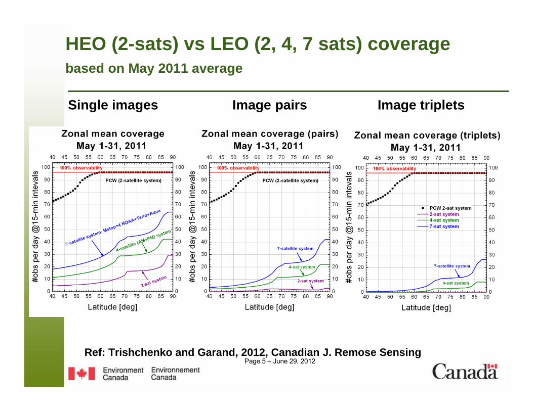
HEO (2-sats) vs LEO (2, 4, 7 sats) coveragebased on May 2011 average

Single images Image pairs Image triplets

Ref: Trishchenko and Garand, 2012, Canadian J. Remose Sensing

– June 29, 2012

Start with real AMV observations

OSE:• OPE system: includes GEO and MODIS AMVs• NO-AMV: OPE, but without AMVs• 3D-Var FGAT• 2 months 27 Dec 2008 to 23 Feb 2009

• Goal:- reassessing AMV impact globally and by region- will allow evaluating the realism of OSSE

– June 29, 2012

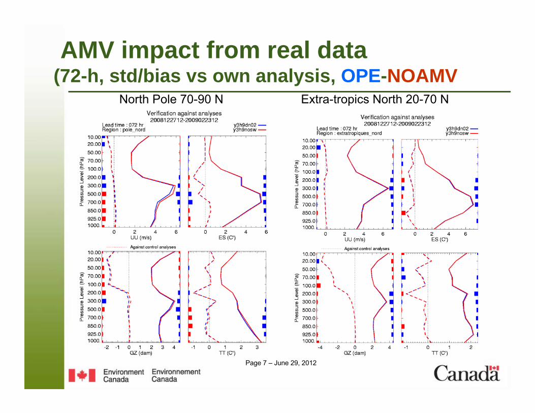
AMV impact from real data (72-h, std/bias vs own analysis, OPE-NOAMV

North Pole 70-90 N Extra-tropics North 20-70 N

– June 29, 2012

Impact of real AMV: 500 hPa TT ano-corOPE-NOAMV

Modest but significant positive impact up to day 4

Extra-tropics North 20-70 N Tropics 20 N – 20 S

______---------- vs control

vs own

– June 29, 2012

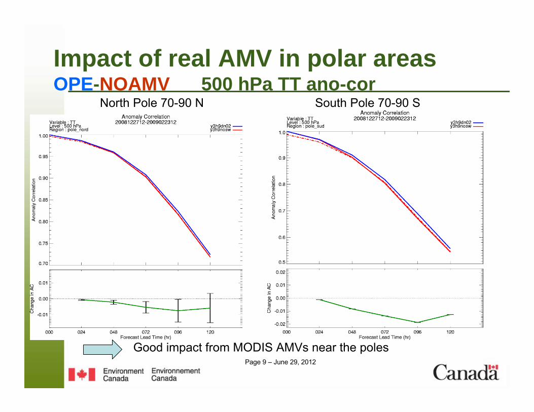
Impact of real AMV in polar areasOPE-NOAMV 500 hPa TT ano-cor

North Pole 70-90 N South Pole 70-90 S

Good impact from MODIS AMVs near the poles

– June 29, 2012

OSSE definition

• Period covered in test cycles (2.5 months):– 15 December 2005 to 28 February 2006

• Simulated from NR all data types assimilated. Positions are those at the same dates in 2008-2009, to include recent types (GPSRO, IASI) not available in 2005-2006.

• All-sky (cloudy) IR radiances were simulated from NR. Clear radiances were selected as done operationally (residual cloud contamination is possible).

• Background check done once for all (same data assimilated in all cycles).

– June 29, 2012

About 4M obs simulated & assimilated(all those of the operational system)

• Conventional- radiosondes & dropsondes, aircrafts- surface reports, buoys, ships- wind profilers

• Satellite- AMVs from Modis Terra/Aqua, 5 GEOs- scatterometrer surface ocean winds- AMSU-A/B, MHS from 8 satellites- hyperspectral IR from AIRS & IASI- GEO water vapor channel from 5 satellites- GPSRO refractivity from 9 satellites

– June 29, 2012

Simulation and assimilation setups

• Assimilation model and system:▪ Operational Global Environmental Multi-scale model (GEM)

– 801x600 (~35 km), 80 levels, top 0.1 hPa ▪ 3D-VAR assimilation, FGAT (First Guess at Appropriate Time) ▪ Cycle starts from 5-day forecast from NR

• ECMWF NR interpolated to GEM grid for validation purposes

– June 29, 2012

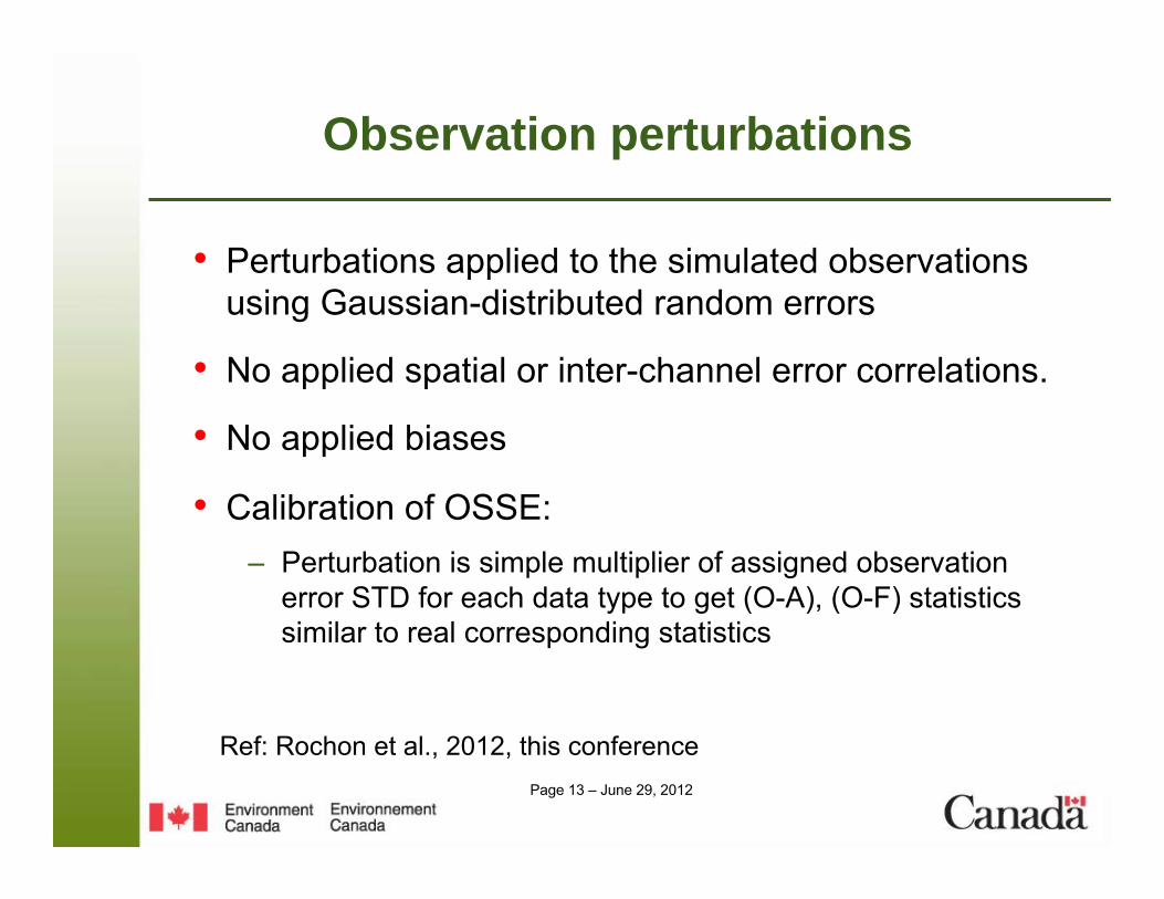
Observation perturbations

• Perturbations applied to the simulated observations using Gaussian-distributed random errors

• No applied spatial or inter-channel error correlations.

• No applied biases

• Calibration of OSSE: – Perturbation is simple multiplier of assigned observation

error STD for each data type to get (O-A), (O-F) statistics similar to real corresponding statistics

Ref: Rochon et al., 2012, this conference

– June 29, 2012

Wind errors assigned in assimilationin comparison to AMV MVD errors

Level hPa

Raob m/s

AMDARm/s

AMVm/s

(O-F) AMV MVD60-90N 20-60N (m/s)

1000 1.6 2.6 3.0 ---- ---925 1.7 2.6 3.0 ---- 1.8850 1.7 2.6 3.0 ---- 1.8700 1.8 2.6 3.5 2.7 3.2500 2.0 2.6 4.5 2.7 3.2400 2.2 3.1 5.0 3.2 3.2300 2.6 3.1 5.5 3.2 3.6250 2.6 3.1 6.0 3.2 3.6200 2.3 3.1 6.0 3.2 3.6150 2.1 3.1 6.0 3.2 3.6100 1.9 3.1 6.0 3.2 3.6

• AMV error inflated in relation to (O-F)• polar MDV lower than extratropics MVD• perturbation is 0.28 AMV obs error

– June 29, 2012

Simulated AMV: NR wind at NR cloud top

11m BTFrom NR

Cloud topPressureWhere TOA tau(cloud)=0.9

Cloud fraction1- tau(cloud)

AMVNR windAt cloudtop

Ref: Garand et al, Atmosphere-Ocean, 2011.

– June 29, 2012

PCW AMV used in assimilation

• thinning at 180 km• no data where cloud free• 50-90 N coverage• allowed range 250-850 hPa• every 6-h• ocean only 50-70 N• same obs error for all AMVs

Conditions similar to operational AMVs except +-3-hwindow for OPE and range 100-700 hPa

– June 29, 2012

Definition of OSSE cycles (3dvar)

OSSE cycles

Comparing current OPE with OPE+ PCW AMV:• PR10: mimics complete OPE system

includes GOES and MODIS AMVs• PCWS: PR10 + PCW AMVs

Comparing NOAMV to adding PCW AMV:• EXP1: PR10 without AMV (no IR radiances by mistake) • EXP2: EXP1 + PCW AMVs (no other AMVs)• EXP3: EXP2 with AMV obs error X 0.7

* EXP1 to be redone with IR radiances assimilated for comparison to PR10 and equivalent denial experiences done with real data

– June 29, 2012

50-90 N

20-50 N

500 hPa anomaly correlation (vs NR) No-AMV PCW-AMV

UU GZ TT

Impact extends to 20-50N region!

– June 29, 2012

Time series of 500 hPa GZ STD vs Nature RunNO-AMV PCW-AMV

20-50 N 50-90 N

Impact as strong in 20-50 N region than 50-90 N 72h-120h

– June 29, 2012

24-h

72-h

120-h

Zonal mean of std difference for temperatureNo-AMV - PCW-AMV

Vs Nature run vs own analysis

Results differsignificanly earlyIn forecast

Results get much closer with time

Positive impact spreadsto lower latitudes (red)

– June 29, 2012

Comparing results vs own analysis and vs NR (50-90 N) NO_AMV-PCW_AMV

24-h

72-h

VS OWN ANALYSIS VS NR ANALYSIS

GZ TT GZ TT

– June 29, 2012

Comparing Simulated OPE to OPE+PCW_AMV(against NR)

50-90 N 20-50 N

Significant gain up to day 3 of ~2h in both regions

– June 29, 2012

Comparing Simulated OPE to OPE+PCW_AMV(against NR) 500 hPa temperature

50-90 N 20-50 N

Gain a 72-h in both regions linked to specific good cases

– June 29, 2012

70-90 N

50-90 N

Nominal AMV error AMV error x 0.7

Lower AMV errorimproves score

Lower AMV errordegrades score

Impact of reducing AMV observation error (500 hPa UU anom-corr)

NO-AMV PCW-AMV

– June 29, 2012

Examination of DFS (% of total per type)

OI (%) = 100 * DFSk/Pk (Courtesy P. Du, P. Gauthier)

ai airs csr iasi mi pr ro sc sf sw amsua amsub ua0

5

10

15

20

25

30

35OSSEREAL_OBS

Obs

erva

tion

influ

enc e

(%)

AIRS IASI SCAT SFC AMV AMSUA B RAOB

– June 29, 2012

Conclusion

• A comprehensive OSSE setup was developed which proves useful fo infer added value of HEO AMVs

• OSE: Real AMVs have modest but consistent positive impact at all latitudes in OPE system up to day 4.

• OSSE: adding PCW AMVs has a significant positive impact up to day 3, not only in region of PCW data (50-90 N) but in midlatitudes as well (20-50 N).

• Validation vs NR or own analysis consistant after day 2 • Gain of predictability of order 1-3h at day 3 in region 20-

90 N.

assimilation impact from satellite wind observations filling … · assimilation impact from...

Documents