asset liability management for tanzania : pension funds by

Afrika StatistikaVol. 13 (3), 2018, pages 1733 –1758.DOI: http://dx.doi.org/10.16929/as/1733.131

Afrika Statistika

ISSN 2316-090XAsset liability management for Tanzania :pension funds by stochastic programming

Andongwisye John1∗, Torbjorn Larsson 2 , Martin Singull3 and Allen Mushi4

1,4Department of Mathematics, University of Dar es salaam2,3Department of Mathematics, Linkoping University

Received : August 15, 2018. Accepted : August 30, 2018

Copyright c© 2018, Afrika Statistika and The Statistics and Probability African Soci-ety (SPAS). All rights reserved

Abstract. We present a long-term model of asset liability management for Tanzaniapension funds. The pension system is pay-as-you-go where contributions are usedto pay current benefits. The pension plan is a final salary defined benefit. Two kindsof pension benefits, a commuted (at retirement) and a monthly (old age) pensionare considered. A decisive factor for a long-term asset liability management is that,Tanzania pension funds face an increase of their members’ life expectancy, whichwill cause the retirees to contributors dependence ratio to increase. We present astochastic programming approach which allocates assets with the best return toraise the asset value closer to the level of liabilities. The model is based on workby Kouwenberg in 2001, with features from Tanzania pension system. In contrastto most asset liability management models for pension funds by stochastic pro-gramming, liabilities are modeled by using number of years of life expectancy formonthly benefit. Scenario trees are generated by using Monte Carlo simulation.Numerical results suggest that, in order to improve the long-term sustainabilityof the Tanzania pension fund system, it is necessary to make reforms concerningthe contribution rate, investment guidelines and formulate target funding ratios tocharacterize the pension funds’ solvency situation.

Key words: Pay-as-you-go pension fund, asset liability management, stochasticprogramming, scenario trees.AMS 2010 Mathematics Subject Classification : 62P05, 90C15.

∗Corresponding author Andongwisye John: [email protected] Larsson : [email protected] Singull : [email protected] Mushi : [email protected]

J. Andongwisye, Larsson T., Singull S. and Mushi A, Afrika Statistika, Vol. 13 (3), 2018,pages 1733 –1758. Asset liability management for Tanzania : pension funds by stochasticprogramming. 1734

Resume. Nous presentons un modele a long terme de gestion actif-passif pour lesfonds de pension tanzaniens. Le systeme de retraite est un systeme de repartitionqui utilise les cotisations pour payer les prestations courantes. Le regime de retraiteest base sur les points du dernier salaire. Deux types de prestations de retraite, unerente viagere (a la retraite) et une rente mensuelle (vieillesse) sont pris en compte.Un facteur decisif pour une gestion actif-passif a long terme est que les fonds depension tanzaniens sont confrontes a une augmentation de l’esperance de vie deleurs membres, ce qui entraınera une augmentation du taux de dependance des re-traites a contributeurs. Nous presentons une approche de programmation stochas-tique consistant a allouer des actifs offrant le meilleur rendement afin d’elever lavaleur de l’actif plus pres du niveau des passifs. Le modele est base sur les travauxde Kouwenberg (2001), avec des caracteristiques du systeme de retraite de la Tan-zanie. Contrairement a la plupart des modeles de gestion actif-passif pour les fondsde pension par programmation stochastique, les passifs sont modelises en utilisantle nombre d’annees d’esperance de vie pour les prestations mensuelles. Les arbresde scenario sont generes a l’aide de la simulation de Monte Carlo. Des resultatsnumeriques suggerent que, pour ameliorer la viabilite a long terme du systeme defonds de pension tanzanien, il est necessaire de proceder a des reformes concer-nant le taux de cotisation, les directives d’investissement et la formulation de ratiosde financement objectifs pour caracteriser la situation de solvabilite des fonds depension.

1. Introduction

A pension is a generic term for single or periodic payments to a beneficiary, whichreplaces a former income of an employee in case of reaching a certain age, or inthe case of disability or death. A pension fund is considered to be an organization,obliged with paying pensions and it has a task of making benefit payments tomembers who have ended their active earnings carrier. The payments to be madeto the retirees must be in accordance with a benefit condition that prescribes theflow of payments to which each member in the fund is entitled.

There are two major kinds of pension fund schemes, known as defined contribu-tion (DC) and defined benefit (DB). A defined contribution scheme specifies howmuch a member will contribute, often as a fixed percentage of salary. The fixedpercentage of the salary is called contribution rate. The benefit is determined bythe size of accumulated contributions in an individual account that participatesin a profit sharing. At an agreed age or state, pension benefits are paid as a lumpsum or as regular payments, depending on contributions as well as development ofinvested funds. A defined benefit scheme specifies a level of benefit, usually basedon salary in relation to near retirement (final salary), or on salary throughoutemployment (career average salary plans). This level is usually defined accordingto a benefit formula as a function of the salary and years of the service. Thecontributions from employer and employee are accumulated to meet the level ofbenefit. Contributions may be increased or decreased depending on investmentperformance or demographic experience. The main difference between DC and DB

Journal home page: www.jafristat.net, www.projecteuclid.org/as


pension schemes is the way in which the financial risk is treated. In DC plans,the financial risk is borne by the contributors. In DB scheme, the financial risk isborne by the sponsors of the scheme. Recently, due to the demographic evolutionand the development of the equity market, DC schemes have become popular inthe global pension market (Gao, 2008).

A pay-as-you-go pension is a system where current benefit payouts for retirees arepaid by using contributions from current members. To be sustainable, it requiresa balance between the benefits paid to the retirees and the contributions madeby the current members. The world demography is however changing rapidlywith increased life expectancy and decreased fertility rate (Johnson, 2004; Batiniet al., 2006), and the retirees population is growing, compared to the workingpopulation, in most countries of the world (Bos et al., 1992). The increasing ratioof retirees to working population is bringing various policy responses. Parametricreforms tinker with pay-as-you-go defined benefit pension schemes by reducingbenefits, and also raising taxes and eliminating the incentives for early retirementwill be necessary.

There are recent applications of Asset Liability Management (ALM) for pensionfunds by stochastic programming for several countries. Dert (1995) studiedasset liability management by chance constraints for Dutch pension funds andKouwenberg (2001) studied multistage stochastic programming for a Dutchpension fund. Dupacova and Polıvka (2009) studied ALM for Czech pension funds,Hilli et al. (2007) for a Finnish pension company, Mulvey et al. (2000) for a TowersPerrin-Tillinghast pension fund in America, and Geyer and Ziemba (2008) foran Innovest Austrian pension fund. Klein Haneveld et al. (2010) studied ALMwith integrated chance constraints for Dutch pension funds while Hussin et al.(2014) studied two-stage stochastic programming using integrated chance con-straints for a Malaysia pension fund. Bogentoft et al. (2001) and Bai and Ma (2009)study ALM with CVaR constraints for Dutch and China pension funds, respectively.

Several studies of the challenges facing pay-as-you-go pension systems due tochanges in demography have been conducted. Among these are Humberto et al.(2016) who studied a sustainability framework for pay-as-you-go pension system.This study forecasts that the net present value of expenditure on pensions inthe US will exceed the net present value of contributions through the period2015 − 2089. Ai et al. (2015) develop a benchmark risk measure for pensionsponsors by obtaining a total asset requirement for sustaining the pension planwith respect to the risk of increased longevity.

We develop an asset liability management for Tanzania pension funds by stochasticprogramming. As an application, the largest pension fund in Tanzania, the Na-tional Social Security Fund (NSSF) is considered. According to the Social SecurityRegulatory Authority (SSRA), this fund has about 44% of the total pension fundspopulation in 2015 and the retirees to contributors dependency ratio is the lowest



among Tanzania pension funds.

The remainder of this paper is organized as follows. The Tanzania pension fundsystem is presented in Section 2. Section 3 outlines an asset liability managementfor pension funds by stochastic programming. The model is developed in Section4 while Section 5 explains the scenario tree generation. Numerical results andsimulations are presented in Section 6 while Section 7 gives the summary andconclusion.

2. Tanzania pension system

The pension fund system in mainland Tanzania is characterized by five pensionfunds serving a small subset of the population. These are Parastatal PublicPension (PPF), Public Service Pension Fund (PSPF), National Social SecurityFund (NSSF), Local Authority Pension Fund (LAPF) and Government EmployeesProvident Fund (GEPF). In year 2015, the system covered 2.14 millions memberswhich was about 4% of the total population and 10% of the working population.All funds were converted to pay-as-you-go defined benefit between 1999 and 2013.These funds are regulated and supervised by the Social Security RegulatoryAuthority (SSRA).

The SSRA was established under the social security regulatory authority Act No. 8of 2008 and amended by Act No. 5 of 2012, with the main objective of supervisingand regulating the social security sector. This authority started its operationsat the end of the year 2010. It may set contribution rates payable to a fund bymembers and minimum benefit payable to its beneficiaries. But before adjustingcontribution rate and minimum benefit payable, the authority should undertakeor cause a fund to undertake actuarial valuation. Currently, the contribution rateis 20% of the monthly salary. An employee commonly pays 5% and the employerpays 15%, while in some funds including NSSF, an employee and employer eachpays 10%.

The five aforementioned pension funds offer different kinds of benefits, on shortand long term. Two of the benefits paid by the funds are commuted and monthlybenefit. Commuted benefit is a part of pension payable as a lump sum at retire-ment. The monthly benefit is the part of pension converted as regular monthlypayments after retirement on the condition of retiree survival. A member whoattains an age of fifty-five years may at any time thereafter opt to retire, but ifhe does not, he may continue be working until the compulsory retirement ageof sixty. To receive pension a member should have contributed for 15 years, thatis, 180 months provided a member has met other conditions set in the enablinglegislation of the respective fund and attained the retirement age. The currentbenefit formula was issued in 2014 by SSRA and aims to offer a commuted benefitof 25% of highest average final salary (average of the highest three salaries in thelast 10 years preceding retirement) for all contributing months of a beneficiary paidat retirement. The monthly benefit aims to a benefit of 75% of average final salary



Table 1: Asset investment limits

Asset Lower limit Upper limitGovernment Security 20% 70%

Real Estate 0% 30%Loans 0% 20%

Fixed Deposit 0% 35%

for all contributing months, paid every month after retirement. This benefit aimsat a minimum pension payable to members not less than 40% of the prescribedlowest minimum wage. The authority may where necessary set rates of indexationof members benefit to the current level of earnings of contributors.

The investment of pension funds had grown up to 7.8 trillion Tanzania shillingsin 2014/15. The Bank of Tanzania in consultation with SSRA issue guidelines re-garding pension funds investment activities. These guidelines prescribe limits forinvestments in various asset categories to foster risk diversification and limit ex-cessive concentration of risk. Pension funds may invest in the following asset cate-gories: fixed deposits, government security, corporate bonds, loans to government,loans to corporate and cooperative societies, equities, property and licensed collec-tive schemes. Since our ALM model is limited to a long-term strategic decision, asmall set of asset categories should be sufficient, as recommended by Kouwenberg(2001). Therefore, we consider four asset categories only, which are governmentsecurity, real estate, loans and fixed deposit. Government security is a low riskasset with high returns, real estate is a low risk asset with low return. Further,loans have high risk and high return while fixed deposit has low risk and high re-turns. The recent investment guidelines were issued by Bank of Tanzania in 2015,as shown in Table 1.

The pension fund may exceed the upper limits in the event of an increase inthe market price of assets, reevaluation, bonus issues or transfer of investmentfrom one category to another provided that, no new investment shall be done forthose categories until such times, when the investments are restored to the limitsprescribed in the guidelines. Such excess should be reported immediately to theBank of Tanzania.

We consider these guidelines to be regulatory and not practical. We therefore modifysome of the limits to make them more practical and suitable for modeling. Sinceloans have high risk, we decrease its upper bound to 10%. We increase the lowerbound for real estate to 20% since it is a low risk asset. Also, pension funds needto participate into real estate activities that directly support their stakeholders(employees and employers). Table 2 displays the modified limits.Table 3 gives the anticipated remaining life expectancy of members of Tanzaniapension funds at different periods of time, by age and sex as given in Isaka (2016).



Table 2: Modified asset investment limits

Asset Lower limit Upper limitGovernment Security 20% 70%

Real Estate 20% 30%Loans 0% 10%

Fixed Deposit 0% 35%

Table 3: Remaining life expectancy of members at different time, by age and sex

Men WomenYear At 20 at 40 At 60 At 20 At 40 At 602013 54.6 37.5 20.8 55.7 39.1 22.22038 57.1 39.2 21.8 58.1 40.4 22.92063 59.7 41.0 22.9 61.2 42.5 24.22088 61.8 42.6 23.9 63.6 44.2 25.4

3. Asset liability management for pension funds by stochastic programming

Stochastic programming is an approach for modeling decision problems thatinvolve parameters that are not known at the time of making decisions. In an ap-plication of stochastic programming, these uncertainties are modeled as randomparameters in a discrete time model with a finite planning horizon (Dupacovaand Polıvka, 2009). Stochastic programming has been proven to be an efficientapproach in designing effective strategies in wealth and asset liability managementin practice (Hilli et al., 2007).

3.1. Multistage stochastic programming

In multistage stochastic programming, decisions xt are taken in time stages t =1, . . . , T . The initial decision x1 is followed by a random realization ξ1, the nextdecision, x2, is followed by the realization ξ2, and so on. A multistage decisionproblem may allow a decision xT at the terminal time such that

x1 → ξ1 → x2 → ...→ xT−1 → ξT−1 → xT (1)

or terminate with the last observation ξT , such that

x1 → ξ1 → x2 → ...→ xT → ξT . (2)

Basing on Shapiro et al. (2009), the sequence ξt for t = 1, . . . , T is a stochasticprocess, and we let ξ[t] = (ξ1, . . . , ξt) denote the information process up to time t.The decision xt taken at stage t depends on the information data ξ[t], but not on thefuture realization, which is the nonanticipativity property, the basic requirement



of stochastic programming .

The generic form of a T-stage stochastic programming problem can be written in anested formulation as

minx1∈X1

f1(x1) + E[

minx2∈X2(x1,ξ2)

f2(x2, ξ2) + E[· · ·+ E

[min

xT∈XT (xT−1,ξT)fT (xT , ξT )

]]], (3)

where E is the expectation operator, the function f1 : Rn1 → R is continuous anddeterministic and the set X1 ⊂ Rn1 is deterministic. Further, xt ∈ Rnt , t = 1, . . . , T ,are decision variables and ft : Rnt × Rmt → R are continuous functions at stagest = 2, . . . , T . The multistage problem is linear if the objective functions and theconstraint functions are linear.

The formulation which is often used in stochastic optimization models, is

minx1,x2,..,xT

E[f1(x1) + f2(x2(ξ[2]), ξ2) + · · ·+ fT (xT (ξ[T ]), ξT )

]subject to x1 ∈ X1,

xt(ξ[t]) ∈ Xt(xt−1(ξ[t−1]), ξt), t = 2, . . . , T. (4)

In this formulation the decision variable xt = xt(ξ[t]), t = 1, . . . , T , is considered asa function of the data process ξ[t] up to time t.

3.2. Scenario tree

In stochastic programming, the uncertainty of parameter values are described bya scenario tree. The scenario tree branches off every random parameter in eachtime stage. This approach requires a finite discrete distribution, that is, a limitednumber of possible values of the random parameters. According to Kouwenberg(2001), the performance of stochastic programming can be improved by choosingan appropriate scenario generation method.

Following Pflug and Pichler (2014), scenario trees are circle free directed graphs,with a unique root, for which the distance of all leaves nodes from the root is equalto T − 1. Scenario trees carry probability valuations on nodes and on arcs.

The tree consists of N nodes and for each node n, except the root, a predecessorpred(n) is defined. The nodes of the tree are dissected into a node set at each stage,called Nt such that

N1 is the root node,NT are terminal nodes (leaves),Nt, t = 2, . . . , T − 1, are intermediate nodes (inner nodes).

For each t = 2, . . . , T and all n ∈ Nt, pred(n) ∈ Nt−1. A scenario s corresponds topath of nodes from the root node to a terminal node in NT .



Fig. 1: Scenario tree for T = 3 stages, with 10 nodes, and 6 scenarios

Figure 1 shows an example of a scenario tree for a process explained above withT = 3 stages, 10 nodes, and 6 scenarios. Stages are presented by t = 1, 2, 3. Theroot node n1 is the predecessor of nodes n2, n3 and n4 at stage t = 2. Each of thenodes at this stage has two successors at stage T = 3. Nodes at stage t = 2 arepredecessors of nodes at stage T = 3.

3.3. Application to asset liability management for pension funds

Asset liability management for a pension fund is a risk management approach,which takes into account the assets and liabilities, in reference to differentrestrictions from policies that can be applied. The main characteristic of financialinstitutions is the solvency, which is the ability to meet long-term obligations. Themanagement of a pension fund should make a decision on acceptable policiesthat guarantee with a high likelihood that the solvency is sufficient during theplanning horizon, which is up to several decades. In order to take sound decisions,the management needs to identify financial risks that may affect the solvency.

The solvency characterization differs from country to country. Some use the ratioof asset value to liability (funding ratio) to define the solvency (Dert, 1995). Whenthe funding ratio equals 100%, it means that the value of the assets will exactlymatch the value of the liabilities. The ratio greater than 100% means over-funding,that is, the fund will have a surplus. But if it is less than 100%, the fund’s assetsvalue will not cover all liabilities. Other countries use defined financial levels tocharacterize the solvency (Hilli et al., 2007). These levels are used as an earlywarning system so that the institution and regulators can take actions before apossible bankruptcy.



Management of assets involve decisions on investments while the liability consistsof future pension payments. The future assets returns, liabilities, streams of con-tributions and benefit payments are unknown at the time of making a decision.Stochastic programming models these uncertainties as random parameters ina discrete time model with a finite planning horizon consisting of time stagest = 1, . . . , T .

At stage t a decision xt, which is selling and buying of assets, is made. The decisionis on the diversification of the current wealth of the fund among I asset categories.The major uncertainty for pension funds is the return of each asset investmentat every time stage. Considering random asset return rates r1t, . . . , rIt at stagest = 1, . . . , T − 1, a random process with a known distribution is formed.The first stage is deterministic and a decision is made by specifying the transactionamounts x1 = (x11, . . . , xI1) in each asset. At stage t, the decision xt = (x1t, . . . , xIt)is a function xt = xt(ξ[t]) of the available information ξ[t] = (ξ1, . . . , ξt) of the dataprocess up to stage t. The sequence of functions xt = xt(ξ[t]), t = 2, . . . , T − 1,defines the implementable policy of the decision process.

The objective may represent the expected utility while the scenario-wise objectivesrepresent discounted sums of utility over time. Sometimes, a part of the objectivemay be interpreted as a penalty function. This is appropriate for the class of port-folio selection problems in which asset liability management falls. Such objectivestend to penalize the violation of goal constraints, such as goals for the solvency ofthe fund.

4. Problem formulation

We here present a multistage stochastic programming model for Tanzania pensionfunds. The sequence of decisions are made for a planning horizon of 50 years. Thestages are indexed by t = 0, . . . , T , where t = 0 denotes the present time and t = Tis the end of the planning horizon. Random realizations at stages are representedby nodes of a scenario tree. We denote by Nt the number of nodes of the scenariotree in stage t. The predecessor of the node n is denoted by n.

There are I asset categories indexed by i. The definitions of parameters and vari-ables are given below.



Deterministic parameters

Xinii Initial amount held in asset i

mini Initial cash position

crlo/up Lower/upper bound for contribution rate

dcrlo/up Lower/upper bound for the decrease/increase of contribution rateFmin Minimum funding ratioF end Required funding ratio at the end of the planning horizonlb/ub Lower/upper bound for portion of asset mixtpi /t

si Transaction cost for purchasing/selling of asset category i

λ Positive parameter for specifying risk aversion

Random parameters

Btn Benefit payment at node n of stage tLtn Liabilities at node n of stage tStn Total salaries of members at node n of stage tritn Rate of return of asset category i at node n of stage t

Decision variables

Xhitn Amount held in asset category i at node n of stage t

Xpitn Amount purchased of asset category i at node n of stage t

Xsitn Amount sold of asset category i at node n of stage t

Atn Asset value at node n of stage tcrtn Contribution rate at node n of stage tcrendn Contribution rate at node n of the end of the horizon, needed to lift

the funding ratio to F end

Ztn Deficit relative to the minimum funding ratio Fmin at node n of stage t

4.1. Asset inventory constraints

These constraints describe the dynamic change of amount in assets investment ineach stage. No rebalance is made (no decision is taken) at the end of the horizon.

Xhi01 = Xini

i +Xpi01 −X

si01, i = 1, . . . , I (5)

Xhitn = (1 + ritn)Xh

i,t−1,n +Xpitn −X

sitn,

n = 1, . . . , Nt, t = 1, . . . , T − 1, i = 1, . . . , I (6)

Here, equation (5) describes the initial amount invested at stage t = 0.



4.2. Cash balance constraints

These constraints specify that the cash inflow is equal to the cash outflow. Thereare two sources of cash inflow, which are contributions from members and sellingof assets. Cash outflow is the benefit paid to retirees and purchasing of assets.Transaction costs for selling and purchasing of assets are incorporated. Borrowingand lending variables are not included since there is a loan asset. There is no cashbalance at the end of the horizon.

cr01S01 +mini +

I∑i=1

(1− tsi )Xsi01 −B01 −

I∑i=1

(1 + tpi )Xpi01 = 0 (7)

crtnStn +

I∑i=1

(1− tsi )Xsitn −Btn −

I∑i=1

(1 + tpi )Xpitn = 0,

n = 1, . . . , Nt, t = 1, . . . , T − 1 (8)

4.3. Total asset value

At the end of each stage, the fund should measure its asset value, which is used tomeasure deficit and the solvency. Asset value is the value of previous period assetholdings and the returns of each asset in the current stage.

Atn =

I∑i=1

(1 + ritn)Xhi,t−1,n, n = 1, . . . , Nt, t = 1, . . . , T (9)

4.4. Goal constraints

The pension fund sets a minimum funding ratio Fmin and defines it as a goal. Atthe end of each stage, the deficit is measured. When the funding ratio is less thanthe minimum funding ratio then the deficit is penalized in the objective function.To assure a final wealth of the pension fund, the funding ratio is restored to thetarget level F end at the end of the planning horizon by setting the contribution rateto crendn .

Atn ≥ FminLt − Ztn, n = 1, . . . , Nt, t = 1, . . . , T − 1 (10)ATn ≥ F endLT − crendn STn, n = 1, . . . , NT (11)Ztn ≥ 0, n = 1, . . . , Nt, t = 1, . . . , T − 1

crendn ≥ 0, n = 1, . . . , NT (12)

4.5. Contribution rates constraints

The level and change of contribution rate are bounded.

crlo ≤ crtn ≤ crup, n = 1, . . . , Nt, t = 0, . . . , T − 1 (13)dcrlo ≤ crtn − crt−1,n ≤ dcrup, n = 1, . . . , Nt, t = 1, . . . , T − 1 (14)



4.6. Asset weight mix boundaries

The asset weight mix is bounded. Bank of Tanzania gives asset mix limits throughspecified investment guidelines as described in the Table 1.

lb

I∑i=1

Xhitn ≤ Xh

itn ≤ ubI∑i=1

Xhitn, n = 1, . . . , Nt, t = 0, . . . , T − 1, i = 1, . . . , I (15)

4.7. Objective

We use the objective function of Kouwenberg (2001), which is to minimize the sumof the average contributions rates, while taking into account the risk aversion ofthe pension fund and the state of the fund at the end of the planning horizon. Riskaversion is modeled with a quadratic penalty on deficits Ztn.

min

T−1∑t=0

( Nt∑n=1

crtnNt

)+ λ

T∑t=1

Nt∑n=1

1

Nt

(ZtnLtn

)2

+

NT∑n=1

crendn

NT(16)

Here, λ is the positive risk aversion penalty parameter.

5. Scenario tree generation

5.1. Asset returns scenarios

Asset returns scenarios provide the information about possible future returns ofassets. Each asset scenario should also include a salary increase in order to trans-form the real expected values of the benefits and liabilities into nominal values.Salaries are the rates of change of GDP per capita of working population as de-scribed by the World Bank. To model asset returns , a vector autoregressive model(VAR) is used as discussed in Kouwenberg (2001).

yt = v +Ayt−1 + ut, t = 1, . . . , T (17)yit = ln(1 + rit), t = 1, . . . , T, i = 1, . . . , I (18)

Here rit is the rate of return of asset i in stage t. The returns of each assetare transformed to ln(1 + rit) to avoid heteroscedasticity problems. Further,yt = (y1t, . . . , yIt)

T is an I × 1 random vector of continuously compounded rates,A is a fixed I × I matrix of coefficients, v = (v1, . . . , vI)

T is a fixed I × 1 vector ofintercept terms allowing of nonzero mean E(yt). Finally ut = (u1t, . . . , uIt)

T is anI-dimensional white noise with E(ut) = 0, E(utu

Tt ) = Σu and E(utu

Ts ) = 0 for s 6= t.

The covariance matrix Σu is assumed to be nonsingular.

To include the number of years between stages, the following relation is incorpo-rated.

rit = (1 + βi)τ − 1 + ritσi

√τ (19)

Here, rit is the rate of return produced by the vector autoregressive model, βi isthe mean return of asset i, σi is the standard deviation of the rate of return ofasset i, and τ is the number of years between stages.



5.2. Liability scenarios

Liabilities depend on expected future benefits. When a member makes a con-tribution, an expected benefit to be paid in future is created. Tanzania pensionfunds pay different kinds of pension benefits. These include maternity, gratuity,education, death gratuity, commuted pension and monthly pensions. In ourwork, only commuted and monthly benefits are considered and other benefits areignored. This simplification is due to the fact that other benefits are significantlysmaller, and it is optimistic with respect to the fund’s sustainability. Commutedpension is a part of benefit paid as a lump sum at retirement while monthlypension is a part of benefit paid in terms of regular payments every month fromretirement until the death of the retiree. These two benefits depend on the numberof months that a member has been contributing to the fund and a retiree’s averageannual earnings in the best three of the last 10 years preceding retirement.

To receive pension benefit a member should contribute for at least 180 months andreach an age of retirement. In 2014 SSRA issued the harmonization rule formulafor commuted and monthly benefits (SSRA, 2014). The commuted benefit, denotedCB, is given by

CB =1

580×m× Sfin × 12.5× 25%, (20)

where m is the number of months a participant has been contributing to thefund, Sfin is the average final salary, 1

580 is the annual accrual factor, 12.5 is thecommutation factor at retirement, and 25% is the commutation rate of the annualfull amount of the pension.

A monthly pension, denoted MB, is given by

MB =1

580×m× Sfin × 75%× 1

12, (21)

where 75% is the commutation rate of the annual full amount of the pension. Inour calculations, the monthly pension is regularly revised to follow the growth inaverage salary for the working population. Also, MB is converted to annual benefitinstead of monthly.

In our calculations, a final annual average salary of a member aged k years in yeart is obtained from

Sfintk = St × (1 + d)60−k. (22)

Here, d is the annual salary growth rate and St is the annual average salary inyear t.

The total expected commuted benefit in year t for members of age k is

CBtk = P 60−kt × nk ×

1

580×mk × Sfintk × 12.5× 25%, (23)



where P 60−kt is the probability of a member aged k years in year t to live 60−k years

more, that is, until retirement, nk is the number of members aged k years in yeart, and mk is the average number of months that members of age k have contributed.

Total expected yearly benefit in year t for members aged k is

MBtk = P 60−kt × nk ×

1

580×mk × Sfintk × 75%× Ep60tk , (24)

where Ep60tk is the remaining life expectancy in years in year t for a member agedk years, when he reaches the age of sixty, as shown in Table 3.

The total expected benefit Btk in year t for members of age k is

Btk = CBtk +MBtk.

Liability is the discounted present value of expected total benefit. The total liabilityin year t is therefore given by

Lt =

59∑k=20

Btk(1 + r)60−k

, (25)

where r = 5% is a discount factor. This factor is in line with other assumptions andmodeling used by World Bank economists (PolicyNote, 2014). In our calculations,we assume that initial members had been creating liabilities before the start of thehorizon.

6. Numerical results

Basing on John et al. (2017) and assumptions therein, we project the futurestatus of the members, that is, how many will survive, retire and being paidcommuted and monthly pensions. We update the status of each member year byyear according to predicted mortality rates before retirement age and expectedlifetime thereafter. This projection shows that the fund is facing a mass increaseof retirees in the long future. The amount of contributions will not cover benefitpayouts.

The projected number of members in future 50 years is shown in the Figure 2a.The projection shows a fast growth in number of members for the first 15 years, toreach around 20% of the working population, and then the number of membersgrows slower.

Figure 2b shows that the number of retirees grows slowly in the beginning of thetime horizon and then grows fast after 35 years. This will cause an increase of theretirees to contributors dependency ratio, as shown in the Figure 2c. The depen-dency ratio starts in the beginning year at around 2% and increases to around 39%,which is very high, at the end of the horizon. This is an adverse situation since the



(a) Members growth (b) Retirees growth

(c) Retirees to contributors ratio

Fig. 2: Projected population

contributions from a 100 members is by far not sufficient to pay benefit payouts for39 retirees.We use the vector autoregressive model as described in Section 5.1 to modelstochastic factors and then this model is in turn used for generating data for thescenario tree. The asset data from NSSF annual reports of 2001 to 2011 are used. As-sets considered in this study are government security (Gs), real estate (Re), loans(Lo) and fixed deposit (Fd). Further, each scenario includes salary (Sa) growth,which is based on the yearly rate of changes of GDP per capita of working popu-lation for 2001 to 2011. Table 4 displays the means and standard deviations of theasset returns and the salary, while Table 5 displays their correlation matrix.To avoid any problem with spurious and unstable asset returns, lagged variablesare not used for the real estate, loans and fixed deposit assets. Estimation of vectorautoregressive coefficients is done by using a least square method as discussed byDrijver (2005) and Dert (1995). The result is displayed in Table 6 while Table 7displays the estimated correlation matrix of the residuals.Monte Carlo simulation together with Cholesky decomposition are used to generatea scenario tree for the stochastic programming model. Cholesky decomposition



Table 4: Means and standard deviations

Mean Std. DevSa 0.0377 0.0112Gs 0.0919 0.0164Re 0.0346 0.0080Lo 0.0647 0.0151Fd 0.0665 0.0233

Table 5: Correlations

Sa Gs Re Lo FdSa 1Gs -0.0159 1Re 0.3700 0.2220 1Lo -0.5090 -0.0139 -0.5330 1Fd 0.2990 0.2780 0.5400 -0.5040 1

Table 6: Coefficients of the vector autoregressive model

Sa ln(1+Sat) = 0.0381 + 0.0651× ln(1+Sat−1) + e1tGs ln(1+Gst) = 0.0885 + 0.0189×ln(1+Gst−1) + e2tRe ln(1+Ret) = 0.0212 + e3tLo ln(1+Lot) = 0.0769 + e4tFd ln(1+Fdt) = 0.0493 + e5t

Table 7: Residual correlations for vector autoregressive model.

Sa Gs Re Lo FdSa 1Gs -0.1799 1Re -0.2261 0.1369 1Lo -0.0899 -0.3379 -0.1589 1Fd 0.1971 0.2781 0.5028 -0.3596 1

is applied to preserve the covariance structure of rate of asset returns. Futurereturns are estimated using equations (17), (18) and (19). The number of yearsbetween stages is 2, 3, 5, 10, 10, 10, and 10 years respectively. The stages contain atree structure with 1, 20, 5, 5, 2, 2, 2, and 2 nodes, which gives 8000 scenarios. Foreach node a different random vector of distribution of residual is used to generate



Table 8: Deterministic parameters

crlo crup dcrlo dcrup Fmin F end B01 tpi /tsi λ mini S01

0.10 0.20 -0.02 0.02 80% 100% 358 0.02 4 3500 4994

the scenario for the asset returns.

To generate the scenario tree for benefit payouts and liabilities, we use the pro-jected fund population displayed in the Figures 2a and 2b. To get the tree shapedstructure, needed for stochastic programming, we use the salary tree, to generatebenefit payouts and liability trees. The stochastic programming model is solved bythe AMPL/Cplex package. It is assumed that the fund has an initial cash positionand holds assets in all categories. The deterministic parameters are given in theTable 8. Cash are in billions Tanzanian shillings.

6.1. First case: using current investment limits

We start by using the investment limit values as specified in Table 1. We set thefunding ratio at the end of the time horizon F end to 100%, which means that theasset value will match liabilities exactly.

First stage decision asset mix:

In order to attain its goal, the fund has to make first stage decisions. We use theinitial asset holding shown in the Figure 3a, in which loans holding is beyond thelimit (see Table 1). This is allowed by Tanzania pension system with some conditionsas stated in Section 2. As shown in the Figure 3b, the model makes a decision ofselling all real estate assets, which have low risk but also have low return comparedto other assets. Also, the model decides to buy more government security and fixeddeposit, which have low risk but high returns, as displayed on Figure 3c, whileholding the initial value of loans. This means that, the first stage decision on assetallocation is to hold government security, loans, fixed deposit as shown in theFigure 3d.

Average contribution rates:

The average contribution rate is 10%, which is the minimal possible, for all stagesbefore the end of the time horizon. At the horizon the fund needs no contributionto raise the funding ratio to F end, as shown in the Figure 4.

Average asset values:

The Figure 5 shows that, the average asset values grow across the time horizonwith an average annual return rate of 8.5%.



(a) Initial holdings (b) Asset sold

(c) Asset bought (d) Asset hold

Fig. 3: First stage decision on asset allocation

Fig. 4: Average contribution rates



Fig. 5: Average asset values

6.2. Second case: using the modified investment limits

We here use modified investment limits as specified in the Table 2. But we stillconsider the assumptions for contribution rate, asset holdings and funding ratioas in the first case.

First stage decision asset mix:

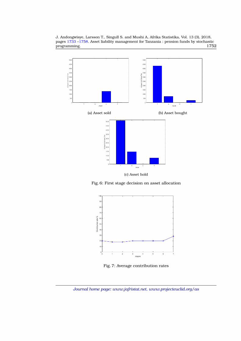
The model makes the first stage decision of selling all of the high risk asset loans, asshown in the Figure 6a. Also, the model decides to buy more government security,real estate and fixed deposit, which are low risk assets, as displayed on Figure 6b.This means that, the first stage decision on asset allocation is to hold governmentsecurity, real estate and fixed deposit, as shown in the Figure 6c.

Average contribution rates:

The average contribution starts at a rate of 20%. At the horizon the average finalcontribution rate to raise the funding ratio to F end is 28%, as shown by the Figure7.

Average asset values:

The Figure 8 shows that, average asset values grow across the horizon with anaverage annual return rate of 8.2%.



(a) Asset sold (b) Asset bought

(c) Asset hold

Fig. 6: First stage decision on asset allocation




Fig. 8: Average asset values

6.3. Funding ratio

Using the modified investment limits specified in Table 2, we study how the fundingratio Frt at stage t of the fund changes. We use the relation

Frt = At/Lt, (26)

where At and Lt are average values for asset values and liabilities, respectively, atstage t. The Figure 9 shows that the funding ratio starts by decreasing fast whiletowards the end of the horizon, the funding ratio raises towards the target fundingratio F end of 100%.

6.4. The difference between contributions and benefit payouts

Since this fund is pay-as-you-go, it is of interest to study the difference betweencontributions and benefit payouts throughout the stages. Basing on the case ofmodified investment limits, according to Table 2, we use the equation (8) to studythe changes in this difference.

crtnStn +

I∑i=1

(1− tsi )Xsitn −Btn −

I∑i=1

(1 + tpi )Xpitn = 0,

n = 1, . . . , Nt, t = 1, . . . , T − 1.

If

crtnStn −Btn < 0 (27)



Fig. 9: Funding ratio

holds, then the fund should sell assets according to the terms (1 − tsi )Xsitn, to pay

benefit payouts rather than buying assets, according to the terms (1 + tsi )Xpitn, for

investment.

Let the average difference between contributions and benefit payouts at stage t bedct, then

dct = crtSt −Bt, (28)

where crtSt is the average contribution at stage t and Bt is the average benefit atstage t. Figure 10 shows that, this difference is first increasing, but in the laststage, it decreases to a large negative value. This means that, at the horizon thefund uses asset values to pay benefit payouts.

6.5. Increasing contribution rate

We here study the effect of increasing contribution rates using the case of modifiedinvestment limits, according to Table 2. We allow the upper bound of the contri-bution rate crup to increase to 25%. As shown by Figure 11, the initial contributionrates are then higher while the rates at stages 5 and 6 are lower, than when themaximal contribution rate is 20%.Considering the Figure 12, the difference between contributions and benefit pay-outs is slightly higher compared to when the maximal contribution rate is 20%.But still at the horizon this value becomes very negative. Hence, before the end ofthe horizon, the fund makes higher surplus which is invested to improve the assetvalues, but towards the end of the horizon assets are instead consumed.



Fig. 10: Difference between contributions and benefit payouts


6.6. The effect of funding ratio on fund’s sustainability

We study the effect of changes in funding ratios for the modified investment limitscase. When the ratios Fmin and F end are both 80%, average contribution rates be-have as in the Figure 4. The difference between contributions and benefit payouts





grows very slowly and then decreases to very negative values after stage 5, whichis earlier than in Figures 10 and 12 . This means that by setting a low fundingratio, contributions will be low, and the fund must use its asset value for the last20 years to pay benefit payouts, which will cause assets to deplete.



7. Conclusion

We present an asset liability management model for Tanzania pension fund bystochastic programming. The pension system is a pay-as-you-go defined benefitwhere the current benefits are paid by using contributions from current membersof the fund. This system is an inter-generation contract which is largely affectedby changes in demography. It is shown that, as the old age population increasesmuch in relation to the number of contributing members, the pension paymentsexceed the contributions, and the asset value is used to pay benefits instead ofbeing investing for covering future benefit payments and liabilities.

Our study suggests that in order to improve the long-term sustainability of theTanzania pension fund system, it is necessary to make reforms concerning con-tribution rates and investment guidelines. Also the authority should formulateconditions for the solvency of funds.

References

Ai, J., Brockett, P. L., and Jacobson, A. F. (2015). A new defined benefit pension riskmeasurement methodology. Insurance: Mathematics and Economics, 63:40–51.

Bai, M. and Ma, J. (2009). The CVaR constrained stochastic programming ALMmodel for defined benefit pension funds. International Journal of Modelling, Iden-tification and Control, 8(1):48–55.

Batini, N., Callen, T., and McKibbin, W. J. (2006). The global impact of demographicchange. IMF Working Paper, 06/9.

Bogentoft, E., Romeijn, H. E., and Uryasev, S. (2001). Asset/liability managementfor pension funds using CVaR constraints. The Journal of Risk Finance, 3(1):57–71.

Bos, E., Vu, M., Levin, A., and Bulatao, R. (1992). World Population Projections1992-1993 Estimates and Projections with Related Demographic Statistics. JohnsHopkins University Press, Baltimore Maryland.

Dert, C. (1995). Asset Liability Management for Pension Funds: A Multistage ChanceConstrained Programming Approach. Ph.D thesis, Erasmus University Rotterdam.

Drijver, S. J. (2005). Asset Liability Management for Pension Funds Using MultistageMixed-Integer Stochastic Programming. Ph.D thesis, University Library Gronin-gen.

Dupacova, J. and Polıvka, J. (2009). Asset-liability management for Czech pensionfunds using stochastic programming. Annals of Operations Research, 165(1):5–28.

Gao, J. (2008). Stochastic optimal control of dc pension funds. Insurance: Mathe-matics and Economics, 42(3):1159–1164.

Geyer, A. and Ziemba, W. T. (2008). The Innovest Austrian pension pund financialplanning model InnoALM. Operations Research, 56(4):797–810.

Hilli, P., Koivu, M., Pennanen, T., and Ranne, A. (2007). A stochastic programmingmodel for asset liability management of a Finnish pension company. Annals ofOperations Research, 152(1):115.



Humberto, G., Maria, D., and Steven, H. (2016). Optimal strategies for pay-as-you-go pension finance: A sustainability framework. Insurance: Mathematics andEconomics, 69:117–126.

Hussin, S. A. S., Mitra, G., Roman, D., Ibrahim, H., Zulkepli, J., Aziz, N., Ahmad, N.,and Rahman, S. A. (2014). An asset and liability management (ALM) model us-ing integrated chance constraints. In AIP Conference Proceedings, volume 1635,pages 558–565. AIP.

Isaka, I. (2016). Updates on Social Security Reforms in Tanzania. Presentation inNBAA Seminar on social security schemes. Dar es Salaam.

John, A., Larsson, T., Singull, M., and Mushi, A. (2017). Projecting Tanzania pen-sion fund system. African Journal of Applied Statistics, 4(1):193–218.

Johnson, R. (2004). Economic policy implications of world demographic change.Economic Review-Federal Reserve Bank of Kansas City, 89(1):39.

Klein Haneveld, W. K., Streutker, M. H., and Van Der Vlerk, M. H. (2010). AnALM model for pension funds using integrated chance constraints. Annals ofOperations Research, 177(1):47–62.

Kouwenberg, R. (2001). Scenario generation and stochastic programming mod-els for asset liability management. European Journal of Operational Research,134(2):279–292.

Mulvey, J. M., Gould, G., and Morgan, C. (2000). An asset and liability managementsystem for Towers Perrin-Tillinghast. Interfaces, 30(1):96–114.

Pflug, G. C. and Pichler, A. (2014). Multistage Stochastic Optimization. Springer.PolicyNote (2014). Public Expenditure Review: Government Pension Obligations and

Contingent Liabilities. World Bank Technical document.Shapiro, A., Dentcheva, D., and Ruszczynski, A. (2009). Lectures on Stochastic

Programming. SIAM, Philadelphia.SSRA (2014). The Social Security Schemes: Pension Benefit Harmonization Rules.

Social security Act No. 8 of 2008 as amended.


asset liability management for tanzania : pension funds by

Documents