State of Ohio Wetland Ecology Group Environmental Protection Agency Division of Surface Water

ASSESSMENT OF WETLANDS IN THE CUYAHOGA RIVER WATERSHED OF NORTHEAST OHIO

Cuyahoga, Geauga, Medina, Portage, Stark, and Summit Counties Ohio EPA Technical Report WET/2007-4

Ted Strickland, Governor Chris Korleski, Director State of Ohio Environmental Protection Agency

P.O. Box 1049, Lazarus Government Center, 50 West Town Street, Columbus, Ohio 43216-1049 ——————————————————————————————————————

ii

This Page intentionally left blank.

iii

Appropriate Citation:

Fennessy, M. S., J. J. Mack, E. Deimeke, M. T. Sullivan, J. Bishop, M. Cohen, M. Micacchion and M. Knapp.

2007. Assessment of wetlands in the Cuyahoga River watershed of northeast Ohio. Ohio EPA Technical

Report WET/2007-4. Ohio Environmental Protection Agency, Division of Surface Water, Wetland Ecology

Group, Columbus, Ohio.

This entire document can be downloaded from the website of the Ohio EPA, Division of Surface Water:

http://www.epa.state.oh.us/dsw/wetlands/WetlandEcologySection.html

Photographs cover page. Top of page: Tare Creek marsh complex (J. J. Mack); Bottom of page: Forest

seep wetland on south valley side of Tare Creek complex (J. J. Mack).

iv

ACKNOWLEDGMENTS

This project was funded by U.S. EPA Wetland Program Development Grant No. CD965114. The principal

authors for this report were Siobhan Fennessy (Kenyon College) and John Mack, (Ohio EPA). Siobhan

Fennessy and Marie Sullivan, (Cuyahoga River RAP) were project managers. Statistical design and sample

selection was performed by Mary Kentula and Tony Olsen (U.S. EPA - EMAP) and Siobhan Fennessy.

Marie Sullivan and Siobhan Fennessy prepared maps and provided GIS support. Field Crew Coordination

was performed by Siobhan Fennessy, Pat Heithaus (Kenyon College), Marie Sullivan and Kelvin Rogers

(Ohio EPA). Special thanks goes to the hard working summer field crew members from the Cuyahoga

River RAP (Susan Haboustak, Samantha Scott, Colleen Sharp, Sonya Steckler), Kenyon College (Carolyn

Barrett, Elizabeth Diemeke, Ellen Herbert, Casey Smith), and Cleveland State University (Beth McGuire).

Thanks to Julie Wolin (Cleveland State University) for coordinating the involvement of Beth McGuire

through the National Science Foundation Research Experiences for Undergraduate Program and for her

participation in this project. Rapid assessment data collection was also performed by Siobhan Fennessy, Pat

Heithaus, Marie Sullivan, Kelvin Rogers, John Mack and Mick Micacchion (Ohio EPA). Wetland

biological assessments were performed by John Mack (plant community), Marty Knapp (macroinvertebrate

community, and Mick Micacchion (amphibian community). Data was managed by Siobhan Fennessy,

Mary Kentula and John Mack. Soil spectral analysis was performed by Matthew Cohen (University of

Florida). Joe Bishop (Penn State Cooperative Wetlands Center) provided land use data for calculation of

the Landscape Development Index. Property owners who permitted access for sampling are also gratefully

acknowledged for their cooperation.

v

TABLE OF CONTENTS

Acknowledgments........................................................................................................................... iv

Table of Contents............................................................................................................................. v

List of Tables .................................................................................................................................vii

List of Figures ...............................................................................................................................viii

Notice to Users................................................................................................................................. x

Abstract ........................................................................................................................................... xi

Introduction...................................................................................................................................... 1

Overview....................................................................................................................................... 1

Wetland Water Quality Standards................................................................................................. 1

Category 1 Wetlands..................................................................................................................... 1

Restorable (modified) Category 2 Wetlands................................................................................. 2

Category 2 Wetlands..................................................................................................................... 2

Category 3 Wetlands..................................................................................................................... 2

Wetland Tiered Aquatic Life Uses................................................................................................ 2

Watershed Overview........................................................................................................................ 4

Landscape setting of Cuyahoga River watershed ......................................................................... 4

The upper, middle, and lower Cuyahoga River ............................................................................ 4

Upper Cuyahoga River watershed ................................................................................................ 5

Middle Cuyahoga River watershed............................................................................................... 5

Lower Cuyahoga River watershed................................................................................................ 5

Methods ........................................................................................................................................... 7

Site selection and Statistical Design ............................................................................................. 7

Assessment Approach ................................................................................................................... 8

Sampling methods - Level 1 Landscape Assessment.................................................................... 8

Land use ........................................................................................................................................ 8

Sampling methods - Level 2 Rapid Assessment ........................................................................... 9

Sampling methods - Level 3 Intensive Assessment .................................................................... 11

Soil and Water Sampling ............................................................................................................ 11

Data analysis ............................................................................................................................... 12

vi

Results............................................................................................................................................ 14

Overview of Results.................................................................................................................... 14

Evaluation of the Ohio Wetland Inventory ................................................................................. 14

Resources Necessary to Assess Wetlands in a HUC8 Watershed .............................................. 14

Level 1 Landscape Assessment................................................................................................... 15

Level 2 Rapid Assessment .......................................................................................................... 17

Causes and Sources of Wetland Degradation ............................................................................. 18

Level 3 Intensive Assessment - Biological Measures................................................................. 20

Level 3 Intensive Assessment - Soils.......................................................................................... 21

Condition of soils and estimates of assimilative capacity of nutrients ....................................... 22

Comparison of Level 1-2-3 Assessment Approach Results........................................................ 22

CART Models - Results.............................................................................................................. 24

Discussion ...................................................................................................................................... 25

Condition of Wetlands in the Cuyahoga Watershed................................................................... 25

Evaluating the Level 1-2-3 Assessment Paradigm...................................................................... 25

Level 1 - Uses and Limitations ................................................................................................... 25

Level 2 - Validation and Sample Size......................................................................................... 27

Level 3 - Sample Size, Verification, and "Fair" Condition......................................................... 28

Buffer Distance, Land Use and Wetland Condition.................................................................... 29

Soil Studies ................................................................................................................................. 29

Study Design - Assessing Wetlands versus Points ..................................................................... 30

Full Implementation of a Statewide Wetland Monitoring and Assessment Program for Ohio... 30

Literature Cited .............................................................................................................................. 32

Appendix...................................................................................................................................... 123

vii

LIST OF TABLES

Table 1. General Wetland Aquatic Life Use Designations ............................................................... 37 Table 2. Special wetland use designations........................................................................................ 38 Table 3. Wetland Tiered Aquatic Life Uses (WTALUs) .................................................................. 39 Table 4. List of land use categories and their associated LDI coefficients ....................................... 40 Table 5a. Soil and water parameters for Level 3 sampling sent to Ohio EPA laboratory ................ 41 Table 5b. Soil and water parameters for soil spectral study collected at random points .................. 42 Table 6. Descriptive statistics for LDI scores ................................................................................... 43 Table 7. Average LDI scores by county for different buffer distances............................................. 43 Table 8. Average LDI scores by antidegradation categories for different buffer distances.............. 44 Table 9. Regression results comparing LDI score to ORAM score by HGM class.......................... 44 Table 10. Percentage of wetlands surrounded by low, medium, or high intensity land uses............ 45 Table 11. Descriptive statistics of wetland area by county and condition category ......................... 46 Table 12. Descriptive statistics of wetland area by TMDL region and condition category.............. 47 Table 13a. Average ORAM scores by five HGM classes for four wetland condition categories..... 48 Table 13b. Average ORAM scores by five plant community classes for four condition categories 48 Table 14. Average number of hydrologic, habitat, or combined stressors by condition category.... 49 Table 15. Percentage of Metric 3e stressors by condition category, county, TMDL region, HGM class, and plant community................................................................................................ 50 Table 16. Percentage of Metric 4c stressors by condition category, county, TMDL region, HGM class, and plant community................................................................................................ 51 Table 17. Average number of stressors and average Weighted Stressor Score from PA Checklist . 52 Table 18. Average values for wetland soil parameters ..................................................................... 52 Table 19. Average ORAM scores by land use intensity categories for different buffer distances ... 53 Table 20. Agreement between LDI and ORAM assessments ........................................................... 53 Table 21. Agreement between LDI and VIBI................................................................................... 54 Table 22. Agreement in condition category assignment between ORAM, Weighted Stressor Score and Wetland Tiered Aquatic Life Uses............................................................................. 55 Table 23. Percentage of wetlands by condition category for LDI, ORAM, Weighted Stressor Score and the VIBI..................................................................................................................... 56 Table 24. ANOVA summary table for comparison of mean ORAM and VIBI scores from Ohio EPA's reference wetland dataset and results from Cuyahoga and Urban Wetland Study 56 Table 25. Summary statistics for ORAM scores on first 50, 100, 125, 150, 200, and 243 points sampled ............................................................................................................................. 57 Table 26. Descriptive statistics of wetland area by TMDL region and condition category.............. 58 Table 27. Summary of staffing scenarios to achieve full rotating basin wetland monitoring........... 59

viii

LIST OF FIGURES

Figure 1. Ecoregions of the Cuyahoga watershed............................................................................. 60 Figure 2. Upper Cuyahoga River Map.............................................................................................. 61 Figure 3. Schematic representation of Upper Cuyahoga River watershed ....................................... 62 Figure 4. Land use/land cover of Upper Cuyahoga River watershed ............................................... 63 Figure 5. Middle Cuyahoga River .................................................................................................... 64 Figure 6. Schematic representation of Middle Cuyahoga River watershed...................................... 65 Figure 7. Land use/land cover in Middle Cuyahoga River watershed.............................................. 66 Figure 8. Lower Cuyahoga River watershed .................................................................................... 67 Figure 9a. Schematic representation of the Lower Cuyahoga River watershed ............................... 68 Figure 9b. Schematic representation of the Lower Cuyahoga River watershed ............................... 69 Figure 9c. Schematic representation of Tinkers Creek portion Lower Cuyahoga watershed........... 70 Figure 10. Land use/land cover in the Lower Cuyahoga River watershed ....................................... 71 Figure 11. GRTS map showing the four hundred initial sampling points ........................................ 72 Figure 12. Preliminary examination of sample points was done using digital aerial photos ............ 73 Figure 13. The fate of wetland points included in this study............................................................ 74 Figure 14. The distribution of wetlands over the seven HGM classes.............................................. 74 Figure 15. Plot showing all sites sampled ordered by ORAM score ................................................ 75 Figure 16. The size distribution of wetlands within major HGM classes ......................................... 75 Figure 17. Scatterplots of LDI-MN score versus LDI-FL score ....................................................... 76 Figure 18. Box and whisker plots of mean LDI scores for each buffer distance .............................. 77 Figure 19. Histograms of LDI scores by different buffer distances.................................................. 78 Figure 20. Scatterplots (and regression line) of LDI scores and ORAM scores ............................... 79 Figure 21. Box and whisker plots of LDI scores for different wetland condition categories ........... 80 Figure 22. Mean LDI scores for each buffer distance stratified by HGM class ............................... 81 Figure 23. Percent variance explained in regression of LDI and ORAM scores .............................. 82 Figure 24A. Percent variance explained in regression of LDI and ORAM scores by HGM class .. 83 Figure 24B. Percent variance explained in regression of forest cover and ORAM scores by HGM class ............................................................................................................... 84 Figure 24C. Percent variance explained in regression of agricultural cover and ORAM scores by HGM class ............................................................................................................... 85 Figure 24D. Percent variance explained in regression of urban cover and ORAM scores by HGM class .............................................................................................................. 86 Figure 25. Pie charts of LDI scores for different buffer distances.................................................... 87 Figure 26A. Frequency histogram of ORAM scores ........................................................................ 88 Figure 26B. Probability plot and Anderson-Darling Normality test................................................. 88 Figure 27A. The distribution of wetlands across the wetland category scheme ............................... 89 Figure 27B. The acreage of wetlands across the wetland category scheme...................................... 89 Figure 28. Pie charts of percentage of wetlands and acreage of wetlands by four counties and four antidegradation condition categories .............................................................................. 90 Figure 29. Pie charts of percentage of wetlands and acreage of wetlands by four TMDL report region and four antidegradation condition categories..................................................... 91 Figure 30. Pie charts of percentage of wetlands and acreage of wetlands by HGM class and four antidegradation condition categories ........................................................................... 92 Figure 31A. Frequency histogram of number of stressors from PA Stressor Checklist ................... 93 Figure 31B. Frequency histogram of Weighted Stressor Score from the PA Stressor Checklist ..... 93

ix

Figure 32A. Box and whisker plots of number of stressors by wetland condition category ............ 94 Figure 32B. Box and whisker plots of Weighted Stressor Score by wetland condition category .... 94 Figure 33A. Percentage of wetlands in poor, fair, good, and excellent condition as determined by the number of stressors from the PA Stressor Checklist.............................................. 95 Figure 33B. Percentage of wetlands in poor, fair, good, and excellent condition as determined by the Weighted Stressor Score from the PA Stressor Checklist...................................... 95 Figure 34A. Scatterplot of number of stressors and ORAM score ................................................... 96 Figure 34B Scatterplot of Weighted Stressor Score and ORAM score ............................................ 96 Figure 35. Percentage of wetlands in LQWLH (poor), RWLH (fair), WLH (good), and SWLH (excellent) condition as determined by Vegetation IBI scores ....................................... 97 Figure 36. Scatterplot of VIBI score versus ORAM score ............................................................... 97 Figure 37. Scatterplot of VIBI score versus number of stressors from the PA Stressor Checklist ... 98 Figure 38. Scatterplot of VIBI score versus Weighted Stressor Score ............................................. 98 Figure 39. Scatterplots of LDI scores and VIBI scores .................................................................... 99 Figure 40. Box and whisker plots of VIBI scores for different land uses intensity classes .............. 100 Figures 41A-K. Bar charts of soil parameters by HGM class, county, condition category, and LDI categories................................................................................................................ 101-111 Figure 42. Box and whisker plots of ORAM scores for different buffer distances .......................... 112 Figure 43. The percent agreement between the Level 1 and Level 2 (ORAM) assessments............ 113 Figure 44. Box and whisker plots average ORAM scores for different Level 1:Level 2 "agreement" categories for different buffer distances.......................................................................... 114 Figure 45. The percent agreement between the Level 1 and Level 3 (VIBI) assessments................ 115 Figure 46. Box and whisker plots of average VIBI scores by different Level 1:Level 3 "agreement" categories for different buffer distances......................................................................... 116 Figure 47A. CART model for ORAM scores for all wetlands ......................................................... 117 Figure 47B. CART model for ORAM scores for depressional wetlands.......................................... 118 Figure 47B. CART model for ORAM scores for riverine wetlands ................................................. 119 Figure 48A. Comparison of mean ORAM scores in Cuyahoga watershed and Urban wetlands in Franklin County with mean scores from Ohio EPA's reference wetland dataset......... 120 Figure 48B. Comparison of mean VIBI scores in Cuyahoga watershed and Urban wetlands in Franklin County with mean scores from Ohio EPA's reference wetland dataset......... 120 Figure 49A. Percentage of wetland resource in four categories based on samples of first 50, 100, 125, 150, 150, 200 and 243 points. .............................................................................. 121 Figure 49B. Percentage of mean ORAM scores in four categories based on samples of first 50, 100, 125, 150, 150, 200 and 243 points. .............................................................................. 121 Figure 49C. Percentage of mean ORAM score standard deviation in four categories based on samples of first 50, 100, 125, 150, 150, 200 and 243 points. ....................................... 122 Figure 49D. Percentage of ORAM score 95% confidence interval in four categories based on samples of first 50, 100,125, 150, 150, 200 and 243 points. ........................................ 122

x

NOTICE TO USERS

Ohio EPA adopted Wetland Water Quality Standards (WWQS; Ohio Administrative Code 3745-1)

regulations in May 1998. These criteria consist of narrative standards, chemical criteria, and a wetland

antidegradation rule that requires wetlands to be categorized by their quality and functions and values.

Category 1 wetlands are wetlands of limited quality, functions or values. Category 2 wetlands are wetlands

of moderate quality, functions, or values but also includes wetlands that have been degraded but a have

reasonable potential for restoration (modified Category 2). Category 3 wetlands are wetlands of superior

quality, functions, or values. A wetland’s category is determined by using the Ohio Rapid Assessment

Method for Wetlands (ORAM) v. 5.0. The ORAM has been calibrated by comparing ORAM scores to

results from detailed assessments.

Ohio EPA has proposed Wetland Tiered Aquatic Life Uses based on a wetland’s ecoregion (Woods et al.

1998), hydrogeomorphic class (Brinson 1993) and dominant plant community. These criteria are derived

from the Vegetation Index of Biotic Integrity and the Amphibian Index of Biotic Integrity. Supporting

documentation for these criteria can be found at:

http://www.epa.state.oh.us/dsw/wetlands/WetlandEcologySection.html

xi

ASSESSMENT OF WETLANDS IN THE CUYAHOGA RIVER WATERSHED

OF NORTHEAST OHIO

M. Siobhan. Fennessy1, John J. Mack2, Elizabeth Deimeke3, Marie T. Sullivan4, Joseph Bishop5, Matthew

Cohen6, Mick Micacchion7, and Marty Knapp7

ABSTRACT

We used an assessment approach combining the USEPA EMAP probabilistic sampling design with existing Ohio wetland assessment tools, including the Ohio rapid assessment method (ORAM), the modified Penn State Stressor Checklist, the Vegetation IBI and the Amphibian IBI, along with a landscape analysis (the Landscape Development Intensity Index) to evaluate the ecological condition of wetlands in the 1,300 km2 Cuyahoga River watershed. Sample sites were selected using the Generalized Random Tesselation Stratified (GRTS) survey design, which provides a geospatially balanced, stratified random sample. The Ohio Wetland Inventory was used as the sample frame for the population of wetlands in the watershed. We evaluated 366 mapped wetland sites and assessed 243 wetlands to determine condition and report on their response to surrounding land-use. Of the 366 sites, we determined that 243 points (66.4 %) were wetlands while the remainder (16.4 %) were characterized as non-wetlands (n = 60) or duplicate points (n = 18). In 12.3 % of the cases (n = 45), field crews were denied site access by property owners. For the wetlands sampled, ORAM scores were normally distributed with a minimum of 16.0, a maximum of 94.0, and a mean of 55.6 (± 14.5 SD). Across the entire watershed, 9.1% of wetlands were in poor condition, 13.2% in fair condition, 51.0% in good condition, and 26.7% in very good condition. There was dramatic decline in the numbers of Category 3 wetlands from the upper parts of the watershed in Geauga county (49.3% of all wetlands sampled), to the middle parts of the watershed in Portage (18.5% and Summit (19.6%) counties, and the near disappearance of Category 3 wetlands in Cuyahoga county (8.3%). Using the Landscape Development Index (LDI), we evaluated the scale at which the effects of land-use are strongest over six buffer widths: 100, 250, 500, 1000, 2000, and 4000 m. ORAM scores were negatively correlated with increasing intensity of land use (high LDI scores) for depressional, riverine, and slope wetlands for each buffer width to a distance of 1000 m, with the strongest correlations for the 100 and 250 m buffer distances. For impoundments, land-use in the first three buffer distances through 500 m did not relate to ORAM score. Overall, land use intensity in the watershed can be characterized as in "low" to "moderately-low". Wetlands in Geauga county had significantly lower LDI scores across most buffer distances than wetlands _________ 1. Department of Biology, Kenyon College, Gambier, Ohio 43022, fennessym@kenyon.edu. 2. Cleveland Metroparks, 4600 Valley Parkway, Fairview Park, Ohio 44126, jjm@clevelandmetroparks.com. 3. Department of Biology, Kenyon College, Gambier, Ohio 43022 4. Cuyahoga River Community Planning Organization, NOACA building, 1299 Superior Avenue, Cleveland, OH 44114, sullivanm@cuyahogariverrap.org. 5. Penn State Cooperative Wetlands Center, 110 Land and Water Research Building, University Park, PA, 16802, jab190@psu.edu. 6. School of Forest Resources and Conservation, University of Florida, 328 Newins-Ziegler Hall, P.O. Box 110410, Gainesville, FL, 32611, mjc@ufl.edu 7. Division of Surface Water, Ohio Environmental Protection Agency, 4675 Homer-Ohio Lane, Groveport, Ohio, 43125 Summit, and Portage counties, particularly for the 1000 m, 2000 m, and 4000 m buffers. The predictive in

xii

in Cuyahoga, Summit, and Portage counties, particularly for the 1000 m, 2000 m, and 4000 m buffers. The predictive power of the Level 1 LDI assessment at the individual site level for all wetlands was low (R2 = 12-17%; p < 0.05) for 100 m to 1000 m buffer classes, and no significant correlations were found at the 2000 m or 4000 m distances. Classification and regression tree analysis indicates that wetland size is also a strong predictor of wetland condition, probably as a function of landscape fragmentation. The utility of the Level 3 data collected in this study was limited by insufficient sample size, restricting our ability to calibrate and validate the Level 1 and 2 protocols with Level 3 data. In particular the Level 3 vegetation data was absent for Category 1, poor condition wetlands. However, the VIBI distribution still had sufficient breadth in disturbance to be highly correlated with the Level 2 assessment tools. The limitation of small sample size was even more of a problem for amphibian data and prevented its use in validation. A secondary objective of this project was to explore key biogeochemical properties of the wetlands being assessed through soil analysis and the development of a soil spectral library. Soil samples were collected at 202 of the wetlands assessed. Soil data showed no consistent trends with condition category. We found depressions contained significantly higher nutrient concentrations (total nitrogen, total phosphorus and total carbon) than riverine sites, and attribute the difference to the accumulation of organic matter in the longer, more stable hydroperiod characteristic of depressional settings. This project demonstrates that the State of Ohio has developed the prerequisite tools required to successfully implement a statewide wetland-monitoring program using statistically- based water quality assessment approaches.

1

INTRODUCTION Overview

The State of Ohio has been developing wetland assessment methods since 1996 with the goal of incorporating statewide wetland monitoring into its existing rotating basin surface water monitoring program. Strategies for designing an effective monitoring program are described in what is known as the “three-tier framework” for wetland monitoring and assessment (U.S. EPA 2006). Wetland monitoring and assessment programs in the U.S. are designed to report on the ambient condition of wetland resources, evaluate restoration success, and report on the success of management activities. The “three-tier framework” is a strategy for designing effective monitoring programs. This approach breaks assessment procedures into a hierarchy of three levels that vary in the degree of effort and scale, ranging from broad, landscape assessments using readily available data (known as Level 1 methods), to rapid field methods (Level 2), to intensive biological and physico-chemical measures (Level 3) (Brooks 2004, Fennessy et al. 2004). Rapid methods are well-suited for assessing the ecological condition of a large number of wetlands in a relatively short time frame.

The overall project objective was to assess the ecological condition of wetlands in the Cuyahoga River watershed 1 in northeast Ohio using existing Ohio wetland assessment tools. There were also several secondary objectives: 1) evaluate using the Landscape Development Index (LDI), Ohio Rapid Assessment Method v. 5.0 (ORAM) and the Amphibian IBI (AmphIBI) and Vegetation IBI for Ohio wetlands (VIBI) for performing watershed scale wetland assessments, and 2) develop standardized protocols for performing future assessments. 1 The Ohio EPA has previously developed a site-suitability model for estimating the land in the Cuyahoga River watershed available for wetland restoration (White and Fennessy 2005).

In addition to these main objectives, the random sample design presented an opportunity for exploring key biogeochemical properties of the wetlands being assessed through the development of a soil spectral library that could then be used in future projects for the rapid characterization of soil parameters. This was accomplished by developing a comprehensive regional soil library of spectral signatures in the visible and near infrared spectrum. With this library, the optical properties of soils can be correlated to soil chemical, physical and biological characteristics of interest, such as total phosphorus and nitrogen, phosphate sorption capacity, or soil enzyme activity. With the development of a soil library, future assessments of wetland soil characteristics in the Cuyahoga basin, and perhaps in the surrounding region, could be completed very cost-effectively and rapidly (i.e., ~$1 per sample, and hundreds of samples a day) (Cohen et al. 2005). Wetland Water Quality Standards

The State of Ohio adopted Wetland Water Quality Standards and a Wetland Antidegradation Rule on May 1, 1998. The rules categorize wetlands based on their quality and impose differing levels of protection based on the wetland's category (OAC rules 3745-1-50 through 3745-1-54). The regulations specify three wetland categories: Category 1, Category 2, and Category 3 wetlands. These categories correspond to wetlands of poor, good and excellent quality. There is also an implied fourth category (fair) in the definition of Category 2 wetlands, i.e. wetlands that are degraded but restorable (modified Category 2). These potentially restorable wetlands are Category 2 wetlands and receive the same level of regulatory protection as other Category 2 wetlands. Category 1 Wetlands Ohio Administrative Code Rule 3745-1-54(C)(1) defines Category 1 wetlands as wetlands which “...support minimal wildlife

2

habitat, and minimal hydrological and recreational functions," and as wetlands which “...do not provide critical habitat for threatened or endangered species or contain rare, threatened or endangered species.” Category 1 wetlands are often hydrologically isolated, have low species diversity, no significant habitat or wildlife use, little or no upland buffers, limited potential to achieve beneficial wetland functions, and/or have a predominance of non-native species. Category 1 wetlands are defined as "limited quality waters" in OAC Rule 3745-1-05(A). They are considered to be a resource that has been so degraded or with such limited potential for restoration, or of such low functionality, that no social or economic justification and lower standards for avoidance, minimization, and mitigation are applied. Category 1 wetlands would include wetlands in "poor" ecological condition. Restorable (modified) Category 2 Wetlands Ohio Administrative Code Rule 3745-1-54(C) states that wetlands that are assigned to Category 2 constitute the broad middle category that “...support moderate wildlife habitat, or hydrological or recreational functions," but also include "...wetlands which are degraded but have a reasonable potential for reestablishing lost wetland functions" creating an implied fourth category of wetlands (modified Category 2 wetlands). Modified Category 2 wetlands include wetlands in "fair" ecological condition. Category 2 Wetlands Ohio Administrative Code Rule 3745-1-54(C)(2) defines Category 2 wetlands as wetlands which "...support moderate wildlife habitat, or hydrological or recreational functions," and as wetlands which are "...dominated by native species but generally without the presence of, or habitat for, rare, threatened or endangered species..." Category 2 wetlands constitute the broad middle category of "good" quality wetlands. In comparison to Ohio

EPA's stream designations, they are equivalent to "warmwater habitat" streams, and thus can be considered a functioning, diverse, healthy water resource that has ecological integrity and human value. Some Category 2 wetlands are relatively lacking in human disturbance and can be considered to be naturally of moderate quality; others may have been Category 3 wetlands in the past, but have been disturbed "down to" Category 2 status. Category 2 wetlands would include wetlands in "good" ecological condition. Category 3 Wetlands Wetlands that are assigned to Category 3 have “...superior habitat, or superior hydrological or recreational functions.” They are typified by high levels of diversity, a high proportion of native species, and/or high functional values. Category 3 wetlands include wetlands which contain or provide habitat for threatened or endangered species, are high quality mature forested wetlands, vernal pools, bogs, fens, or which are scarce regionally and/or statewide. Category 3 would include wetlands of "excellent" condition. Wetland Tiered Aquatic Life Uses The State of Ohio has proposed draft rules which would revise OAC Rules 3745-1-50 to -54 and include an expansion of the OAC Rule 3745-1-53 with Wetland Tiered Aquatic Life Uses (WTALUs) (Tables 1, 2, and 3). The WTALUs generally correspond to the antidegradation categories with the exception that a wetland can be degraded but still exhibit a residual function or value at moderate or high levels such that it is Categorized as Category 2 or 3 but has a lower WTALU use designation. Narrative WTALU categories based on the Vegetation IBI were first proposed in Mack (2001) and have been subsequently updated (Mack 2004b; Mack and Micacchion 2006) and are summarized in Table 1. WTALUs have also been proposed using the Amphibian IBI. In addition to the tiered uses, special uses (values or

3

ecological services) provided by wetlands can be assigned (Table 2). The WTALUs were developed by partitioning the 95th percentile of VIBI scores for that TALU category into sextiles and combining the sextiles into the 4 aquatic life use categories proposed as numeric biological criteria for Ohio wetlands: limited quality wetland habitat (LQWLH) (1st and 2nd sextiles), restorable wetland habitat (RWLH) (3rd and 4th sextiles), wetland habitat (5th sextile), and superior wetland habitat (SWLH) (6th sextile). Numeric TALUs (biological criteria) for Ohio wetlands were developed based on VIBI scores, ecoregion, landscape position, and plant community (Table 3). In the context of this study, the WTALUs were used as true wetland condition categories for evaluating the results of the Level 1, 2, and 3 assessments.

4

WATERSHED OVERVIEW2 Landscape setting of Cuyahoga River Watershed The Cuyahoga River basin drains 2107 km2 (813 mi2) and includes 1963 km (1220 mi) of streams spanning parts of Cuyahoga, Geauga, Portage, and Summit counties with minor amounts of the watershed located in Medina and Stark Counties, emptying into Lake Erie at Cleveland. The Cuyahoga River is one of the few rivers in the world that changes flow direction (south then north), creating a U-shaped watershed. Land use patterns vary greatly from the upper basin (forest-agricultural-rural) to the lower basin (densely urban-industrial). Agriculture is still the predominant land use in the upper basin, and while less prevalent in the middle basin, soils in the Middle Cuyahoga are highly erodable and can cause significant sedimentation and nutrient loadings to streams and wetlands. Resource extraction (e.g. sand and gravel mining) and hydromodification of streams and wetlands are localized throughout the basin, rather than widespread as in western Ohio. The waters of heavily populated areas of the middle and lower basin are strongly influenced by urban and construction site runoff, industrial and municipal point sources, combined sewer overflows, and land disposal of waste. The basin is located in the Erie-Ontario Drift and Lake Plains (EOLP) ecoregion (Woods et al. 1998) which is part of the glaciated Allegheny Plateau (Figure 1). The EOLP ecoregion is a glacial plain that lies between the unglaciated Allegheny Plateau region to the south and the relatively flat, more fertile, Eastern Corn Belt Plain ecoregion to the west. It is

2 Text from this section is drawn liberally

(with thanks to the authors of those reports) from the following Ohio EPA Reports: Total Maximum Daily Loads for the Upper Cuyahoga River, Total Maximum Daily Loads from the Middle Cuyahoga River, and Total Maximum Daily Loads for the Lower Cuyahoga River available at http://www.epa.state.oh.us/dsw/tmdl/index.html.

characterized by glacial formations that can have significant local relief and has a mosaic of cropland, pasture, woodland and urban areas. Soils are mainly derived from glacial till and lacustrine deposits from former pro-glacial lakes. There are five subregions with the EOLP, three of which are significant in the Cuyahoga watershed: Low Lime Drift Plain (rolling landscape of low rounded hills with scattered end-moraines and kettles with lower fertility soils than the till plains to the west), Erie Gorges (steep dissected areas along Chagrin, Cuyahoga and Grand Rivers with many rock exposures, and the Summit Interlobate Area (a region of numerous lakes, wetlands, sphagnum bogs, sluggish streams, kames, and kettles with outwash derived sand and till soils). Many of the glacial features characteristic of the EOLP ecoregion are found in the Cuyahoga River watershed. The northern and eastern boundaries of the watershed are largely defined by terminal moraines. The retreating glaciers buried ancient river valleys with glacial outwash. The river generally follows the course of the buried ancient river valleys but does traverse a ridge of erosion-resistant sandstone near Akron which caused the southerly flowing river to form falls and cascades at Cuyahoga Falls and to turn northwest at the confluence of the Little Cuyahoga River just north of Akron. The river then winds through the outwash terraces, till plains, till ridges, and the Erie Gorges zones in the Cuyahoga Valley National Park before passing through a narrow band of flat lake plain in Cleveland.

The upper, middle, and lower Cuyahoga River The Cuyahoga River basin has been divided by Ohio EPA into three sub-basins for stream TMDL purposes and these sub-basins are also useful for characterizing the amount, type, and quality of the wetland resource in the Cuyahoga watershed: the upper Cuyahoga from the headwaters to the Lake Rockwell dam; the middle Cuyahoga from below the Lake Rockwell

5

dam to the Munroe Falls dam; and the lower from below Munroe Falls dam to the mouth at Cleveland and Lake Erie. Upper Cuyahoga River Watershed The upper Cuyahoga watershed drains 534 km2 (208 mi2) with 565 km (351 mi) of principal streams (Figure 2). It originates in northeastern Geauga County and flows southwest to Kent through relatively hilly kame and kettle topography. This area is well known as a hotspot of rare and listed plant and animal species. Based on Ohio EPA’s wetland reference work since 1996, this region is also home to one of the largest and highest quality wetland complexes remaining in the state of Ohio. Figure 3 is a schematic of the upper watershed showing locations of point sources, tributaries, reservoirs and large wetland areas. Land use in the upper basin is primarily forest and agriculture (Figure 4). Approximately 12% of the land in the upper Cuyahoga basin is owned by the City of Akron and was purchased, in many instances decades ago, to protect its drinking water sources. Many of the largest and best quality wetland complexes on the Cuyahoga floodplains are now owned and protected by Akron. A 40 km (25 mi) segment of the Cuyahoga River from the Troy-Burton Township line to State Route 14 in Portage County has been designated a State Scenic River and several stream segments are designated State Resource Waters. Three large water supply reservoirs for the City of Akron are located in the upper basin: the 173 ha (428 ac) East Branch Reservoir, the 627 ha (1550 ac) LaDue Reservoir, and the 253 ha (625 ac) Lake Rockwell Reservoir, where the Akron drinking water plant is located. Middle Cuyahoga River Watershed The middle Cuyahoga River is located northeast of Akron and covers portions of Portage, Summit, and Stark Counties (Figure 5). It drains 350 km2 (135 mi2) and extends from the Lake Rockwell reservoir northeast of the City of Kent and flows through the urban areas of Kent

and Munroe Falls. The downstream boundary of the middle watershed is Waterworks park in Cuyahoga Falls. A major tributary is Breakneck Creek. A large portion of the wetland resource in The middle Cuyahoga is located in the Breakneck Creek watershed (eastern and southern Portage County). Figure 6 is a schematic of the middle watershed showing locations of point sources, tributaries, reservoirs and large wetland areas. The middle Cuyahoga is characterized by glacial formations and in general, low gradients and velocities. Land use in the western half of the middle Cuyahoga River watershed is urban and suburban; in the Breakneck Creek region of eastern Portage County, agriculture, forest, and wetland land uses predominate (Figure 7). Lower Cuyahoga River Watershed

The lower Cuyahoga River is located predominately in Cuyahoga, Medina and Summit Counties with a very small area in Geauga County (Figure 8). It drains 1217 km2 (470 mi2) from the Waterworks Park in Cuyahoga Falls to Lake Erie in downtown Cleveland, and includes the heavily urbanized Little Cuyahoga River sub-basin in Akron. Figures 9a, 9b, and 9c are a schematic of the middle watershed showing locations of point sources, tributaries, reservoirs and large wetland areas. The lower Cuyahoga is characterized by its passage through the expansive valley of the Cuyahoga Valley National Park (Erie Gorges subregion) and by the extensive and pervasive influence of current and historical industry and urbanization associated with Cleveland and Akron (Figure 10). The lower Cuyahoga has been identified as an Area of Concern by the International Joint Commission and has been the subject of extensive planning and restoration under the auspices of the Cuyahoga River Remedial Action Plan (Cuyahoga River RAP). The Cuyahoga River was also designated an American Heritage river in 1998. Cleveland and Summit County metroparks both have extensive land holdings in

6

the lower Cuyahoga. The lower Cuyahoga also includes

Tinkers Creek, the largest tributary in the entire Cuyahoga watershed (Figure 9c). Tinkers Creek drains 250 km2 (96 mi2) and its watershed includes portions of 4 counties (Cuyahoga, Geauga, Portage Summit). The upper part of the Tinkers Creek watershed has extensive complexes of wetlands which are very similar to the wetland complexes of the upper Cuyahoga watershed in appearance and genesis. Lower Tinkers Creek transitions from a "wetland stream" to a more classic riffle-pool stream as it passes Twinsburg, Ohio and moves into the Tinkers Creek gorge before debauching into the mainstem Cuyahoga.

7

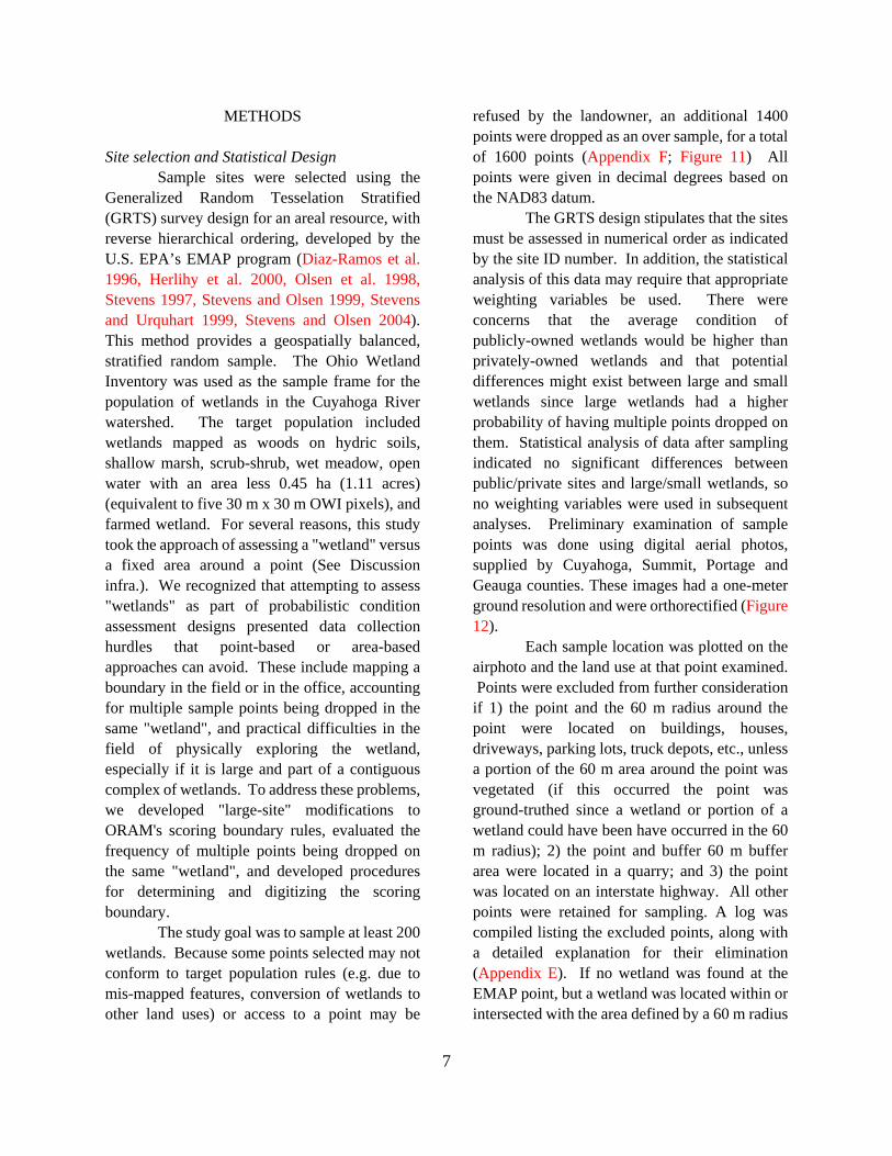
METHODS Site selection and Statistical Design

Sample sites were selected using the Generalized Random Tesselation Stratified (GRTS) survey design for an areal resource, with reverse hierarchical ordering, developed by the U.S. EPA’s EMAP program (Diaz-Ramos et al. 1996, Herlihy et al. 2000, Olsen et al. 1998, Stevens 1997, Stevens and Olsen 1999, Stevens and Urquhart 1999, Stevens and Olsen 2004). This method provides a geospatially balanced, stratified random sample. The Ohio Wetland Inventory was used as the sample frame for the population of wetlands in the Cuyahoga River watershed. The target population included wetlands mapped as woods on hydric soils, shallow marsh, scrub-shrub, wet meadow, open water with an area less 0.45 ha (1.11 acres) (equivalent to five 30 m x 30 m OWI pixels), and farmed wetland. For several reasons, this study took the approach of assessing a "wetland" versus a fixed area around a point (See Discussion infra.). We recognized that attempting to assess "wetlands" as part of probabilistic condition assessment designs presented data collection hurdles that point-based or area-based approaches can avoid. These include mapping a boundary in the field or in the office, accounting for multiple sample points being dropped in the same "wetland", and practical difficulties in the field of physically exploring the wetland, especially if it is large and part of a contiguous complex of wetlands. To address these problems, we developed "large-site" modifications to ORAM's scoring boundary rules, evaluated the frequency of multiple points being dropped on the same "wetland", and developed procedures for determining and digitizing the scoring boundary.

The study goal was to sample at least 200 wetlands. Because some points selected may not conform to target population rules (e.g. due to mis-mapped features, conversion of wetlands to other land uses) or access to a point may be

refused by the landowner, an additional 1400 points were dropped as an over sample, for a total of 1600 points (Appendix F; Figure 11) All points were given in decimal degrees based on the NAD83 datum.

The GRTS design stipulates that the sites must be assessed in numerical order as indicated by the site ID number. In addition, the statistical analysis of this data may require that appropriate weighting variables be used. There were concerns that the average condition of publicly-owned wetlands would be higher than privately-owned wetlands and that potential differences might exist between large and small wetlands since large wetlands had a higher probability of having multiple points dropped on them. Statistical analysis of data after sampling indicated no significant differences between public/private sites and large/small wetlands, so no weighting variables were used in subsequent analyses. Preliminary examination of sample points was done using digital aerial photos, supplied by Cuyahoga, Summit, Portage and Geauga counties. These images had a one-meter ground resolution and were orthorectified (Figure 12).

Each sample location was plotted on the airphoto and the land use at that point examined. Points were excluded from further consideration if 1) the point and the 60 m radius around the point were located on buildings, houses, driveways, parking lots, truck depots, etc., unless a portion of the 60 m area around the point was vegetated (if this occurred the point was ground-truthed since a wetland or portion of a wetland could have been have occurred in the 60 m radius); 2) the point and buffer 60 m buffer area were located in a quarry; and 3) the point was located on an interstate highway. All other points were retained for sampling. A log was compiled listing the excluded points, along with a detailed explanation for their elimination (Appendix E). If no wetland was found at the EMAP point, but a wetland was located within or intersected with the area defined by a 60 m radius

8

of the point (width of two LandSat pixels), then new coordinates were taken at the approximate point where the wetland boundary was closest to the original EMAP point. The new point (termed the "modified EMAP point") was also recorded by indicating its location on the high- resolution aerial photos included in each site folder. If more than one wetland was located within or intersected with the area defined by the 60 m radius circle then the wetland closest to the original EMAP point was sampled. Assessment Approach

Recent approaches to wetland assessment have advocated a multi-level approach which incorporates assessments based on landscape (remote sensing) data (level 1), on-site but “rapid” methods using checklists of observable stressors and other observable wetlands features (level 2), and intensive methods where quantitative floral, faunal, and/or biogeochemical data is collected (level 3) (USEPA 2006; Brooks 2004; Fennessy et al. 2004, 2007). We collected four types of data: 1) GIS data (land use information and other information obtained from existing geographic information system data layers); 2) rapid assessment data obtained from a site visit and recorded on a background information form, a wetland determination form, the Penn State Stressor Checklist (Brooks 2004) and scores from the Ohio Rapid Assessment of Wetlands v. 5.0 (Mack 2001) (Appendix A); 3) quantitative ecological data on vegetation, amphibian, macroinvertebrate assemblages and soil and water chemistry data (at 10% of the sites sampled); and 4) soil chemical, physical and spectral data at 202 of the 242 wetlands assessed. Sampling methods - Level 1 Landscape Assessment

Wetland sample points were selected using the Ohio Wetland Inventory (OWI) database (ODNR 1988). The OWI maps used LandSat satellite data (30 m x 30 m pixels) and

presence of hydric soils to produce the OWI maps. The satellite data reflect conditions at the time that LandSat Thematic Mapper data was acquired (May 1987 for northeast Ohio). The accuracy of the OWI map was evaluated in the field by determining 1) whether or not a wetland actually existed at the point, 2) if a wetland was not located at the point, was a wetland(s) located within a 60 m radius (2 times the pixel width) of the point, and 3) if a wetland was located, was it of the same type as indicated for that location on the OWI. This represented the first systematic field check of the accuracy of the OWI. Handheld geographic position system units, with an accuracy of 0.5 m to 5 m, were used to determine the latitude and longitude of wetlands sampled in this study. Land Use Land-use surrounding the wetland sites included in this study was characterized using the Ohio Digital land-use survey database. Land-use was classified into the following categories (Frohn 2005): 1) forest (a combination of evergreen and deciduous forest cover); 2) pasture (areas of grasses, legumes, or grass-legume mixtures planted for livestock grazing or the production of seed or hay crops); 3) crop (areas used for the production of crops such as corn, soybeans, and wheat); 4) residential (includes both heavily built up urban centers (high intensity residential) and areas with a mixture of constructed materials and vegetation (low intensity residential) and included apartment complexes, row houses, and single-family housing units); 5) commercial (includes infrastructure (e.g. roads, railroads, etc.) and all highways and all developed areas not classified as residential); 6) wetland (a combination of wooded wetland and herbaceous wetland cover); 7) open water; and 8) bare /mined lands.

Upon completion of all field work we used ArcGIS v. 9.0 to digitize all wetland boundaries as indicated by field teams on the airphoto of the site. We then characterized

9

land-uses at various distances beyond the wetland perimeter. We evaluated land-use at distances of 100 m, 250 m, 500 m, 1000 m, 2000 m and 4000 m from the scoring boundary of each site (Houlahan and Findlay 2004). The percent land use for each buffer distance was calculated starting at the wetland perimeter, so the actual area of each land-use type varies with the size of the wetland.(Brooks et al. 2004; Rheinhardt et al. 2006, Wentworth 2006). State-wide land cover data for Ohio, available from Frohn (2005), were used to calculate land cover characteristics. The composition of each land cover class as well as a series of landscape metrics were calculated using a specifically programmed ArcView 3.3 (ESRI 2002) project that automates the processing of multiple polygons (Bishop & Lehning 2007). The program incorporates the landscape metrics included with the ArcView extension software Patch Analyst (Rempel 2007) with several more standard geographic information system (GIS) functions that provide for buffering designated distances away from selected polygons. For this study, the polygons are the digitized wetlands boundaries that were sampled. The program was used to calculate all metrics from within each wetland boundary as well as all specified buffer distances listed above.

Land-use proportions were converted to a Landscape Development Intensity (LDI) index which integrates the impacts of human land use on a given site (Brown and Vivas 2005). The LDI scores were calculated based on assignment of land-use coefficients (Table 4). Coefficients were calculated as the normalized natural log of emergy per area per time, a measurement used to quantify human activity (Brown and Vivas 2005). In terms of the LDI index, emergy is energy corrected for different qualities and includes all non-renewable energies, such as electricity and water. The LDItotal is calculated as a weighted average, such that:

LDItotal = ∑ %LUi * LDIi.

where, LDITotal = the LDI score, %LUi = percent of total area in that land use i, and LDIi = landscape development intensity coefficient for land use i (Brown and Vivas 2005). What is unique to this calculation is that it integrates all land-uses into one score rather than looking at each land-use separately. By using this method (level 1 assessment) in combination with the level 2 and 3 assessments, we could evaluate the response of wetland ecosystems as the human impact on surrounding land-use increases. The LDI index was calculated for each of the six buffer distances by analyzing the different land-uses from the wetland boundary edge. We classified LDI scores to correspond to four wetland condition categories by quadrisecting the 95th percentile of LDI scores for each buffer distance. We also classified into general land-use categories ("natural", "agriculture", and "urban") for simplicity in some analyses: natural (LDI scores of 0-100), agricultural (100-350), and urban (>350). Two different sets of LDI coefficients were used in the analysis: coefficients that were developed for the land uses and climatic conditions of southern Minnesota (Brandt-Williams and Campbell 2006) and a second set of coefficients calculated for Florida (Brown and Vivas 2005) (Table 4). The two sets of coefficients are scaled differently, so their absolute values are not comparable. The LDI score using the Minnesota coefficients can range from 0 to 465; the score using the Florida coefficients can range from 1 to 10. We multiplied the Florida scores by 100 to put them on approximately the same scale as the Minnesota scores. Because of the extremely high correlation between the scores from the two sets of coefficients (see Results), and the fact that climate and land use patterns in Minnesota are more similar to those in Florida, we only used the LDI coefficients for Minnesota in all of our level 1 analyses. Sampling methods - Level 2 Rapid Assessment

10

The ORAM assessment was performed at each wetland point in accordance with the Ohio Rapid Assessment Method for Wetlands v. 5.0, User's Manual and Scoring Forms, Ohio EPA Technical Report WET/2001-1. In addition to ORAM, the Penn State Stressor Checklist (also a Level 2 condition assessment) was completed at each site (Brooks 2004). The Checklist is made up of a set of indicators used to identify probable stressors, such as sedimentation, hydrologic modification, and habitat fragmentation. Data was collected in accordance with all documentation on the appropriate use of the stressor checklist. A Background Field Data form was also completed at each site. Finally, a streamlined Routine Wetland Delineation Form (Environmental Laboratory 1987) was completed to confirm that a jurisdictional wetland was sampled at each location. All forms were completed using the EMAP protocol for handling data forms.

Wetlands were located on the ground using the GPS device and orienteering to the point. Upon arrival at the EMAP point a determination was made as to whether or not the point was within a wetland. If the point was within a wetland, then this point (location) was, by definition, located inside the wetland’s “scoring boundary.” The scoring boundary (assessment unit) was defined by rules outlined in the ORAM v. 5.0 User's Manual (Mack 2001) as follows:

1. Boundaries between contiguous or connected wetlands were established where the volume, flow, source, or velocity of water moving through a wetland changed significantly. Areas with of the same HGM class or with a high degree of hydrologic interaction were included within the same scoring boundary. In many instances, especially for small, depressional wetlands the scoring boundary was the same as the jurisdictional boundary.

2. Boundaries were also established between contiguous wetlands of different HGM classes, e.g. between contiguous slope and

riverine wetlands. 3. Wetlands that form a "patchwork" on

a landscape were scored together (the wetlands were usually 0.4 ha (1 ac.) in size, part of a mosaic of wetlands that were usually less than 30 m (100 ft) apart, and more than 50% of the assessment area was defined as wetland using the 1987 Delineation Manual (Environmental Laboratory 1987).

4. Scoring boundaries were established without regard to property boundaries or boundaries between political jurisdictions.

5. Scoring boundaries were established without regard to roads or railroad embankments provided there was a surface water connection between the two parts of the wetland at least some time during the year.

6. Scoring boundaries of wetlands fringing lakes and reservoirs were established around the entire lake or reservoir and all of its fringing wetlands where the area of open water was less than 8 ha (20 ac.); Scoring boundaries were established around fringing wetlands separately where the area of open water around the lake or reservoir was greater than 8 ha.

7. Scoring boundaries of riverine wetlands were established where a) more than 60 m (200 ft) of non-wetland riparian corridor separated the two wetlands, b) more than 60 m of river channel separated wetlands on either side of a river (except as modified in No. 8 below), or c) at the point where a narrow (<15 m) fringe of wetlands along a stream extending for more than 60 m expands into a broader wetland.

8. In addition to these rules, several supplemental "large-site" rules were developed specifically for this project because of the many very large wetland complexes in the upper Cuyahoga watershed. Where the point fell in a wetland >20 ha (50 ac) in size and this wetland was contiguous to other large wetland areas, streams or roads that bisected the wetland complex were allowed to be used to define assessment unit boundaries.

If no wetland was present within the 60

11

m radius area, the type of land use found at the original EMAP point was recorded as follows: 1) the site was developed and there was no way to know whether a wetland existed there originally or not; 2) the site was farmed, or was otherwise vegetated, and a soil sample collected to a depth of 10 cm using a push corer indicated that hydric soils were not present; 3) the site was farmed, or was otherwise vegetated, and a soil sample collected to a depth of 10 cm using a push corer soil core indicates that hydric soils were present; 4) a determination could not be made. Sampling methods - Level 3 Intensive Assessment

Vegetation. A plot-based vegetation sampling method was used to sample wetland plant communities (Peet et al., 1998). Sampling was performed in accordance with Field Manual for Vegetation Index of Biotic Integrity v. 1.3 (Mack 2004c). At most sites, a “standard” 20 m x 50 m plot was established (0.1 ha). The location of the plot was qualitatively selected by the investigator based on site characteristics and rules for plot location (Mack 2004c). Presence and areal cover was recorded for herb and shrub stratums; stem density and basal area was recorded for all woody species >1m. Percent cover was estimated using cover classes of Peet et al. (1998) (solitary/few, 0-1%, 1-2.5%, 2.5-5%, 5-10%, 10-25%, 25-50%, 50-75%, 75-90%, 90-95%, 95-99%). Woody stems were recorded using diameter classes of Peet et al. (1998) (0-1 cm, 1-2.5 cm, 2.5-5 cm, 5-10 cm, 10-15 cm, 15-20 cm, 20-25 cm, 25-30 cm, 30-35 cm, 35-40 cm, >40 cm stems individually measured). The midpoints of the cover and diameter classes were used in all analyses. Other data collected included standing biomass (g/m2 from eight 0.1m2 clip plots) and various physical variables (e.g. % open water, depth to saturated soils, amount of coarse woody debris, etc.). A soil pit was dug in the center of every plot and soil color, texture, and depth to saturation were recorded. Amphibians and Macroinvertebrates. Funnel traps were used in sampling both the

macroinvertebrate and amphibians present in wetlands. Sample methods followed macroinvertebrate and amphibian IBI protocols in Micacchion (2004) and Knapp (2004). Funnel traps were constructed of aluminum window screen cylinders with fiberglass window screen funnels at each end. The funnel traps were similar in shape to commercially available minnow traps but with a smaller mesh-size. Ten funnel traps were placed evenly around the perimeter of the wetland and the trap location marked with flagging tape and numbered sequentially. Traps were set at the same location throughout the sample period. Each wetland was sampled three times between March and July. Some sites did not have sufficient water present by the 2nd or 3rd trapping run and were only trapped 1-2 times. Traps were unbaited and left in the wetland for twenty-four hours in order to ensure unbiased sampling for species with diurnal and nocturnal activity patterns. Upon retrieval, the traps were emptied by everting the funnel and shaking the contents into a white collection and sorting pan. Organisms that could be readily identified in the field (especially adult amphibians and larger fish) were counted and released. The remaining organisms were transferred to wide-mouth one liter plastic bottles and preserved with 95% ethanol. Laboratory analysis of the funnel trap macroinvertebrate and fish samples followed standardized Ohio EPA procedures (Ohio EPA 1989). Amphibian analysis was performed using the keys of Walker (1946) and Pfingsten and Downs (1989).

Soil and Water Sampling

Water sampling. At all level 3 sites, a grab sample was collected and analyzed for the parameters listed in Table 5a. Field grab samples were analyzed at the Ohio EPA laboratory. Grab samples were collected by directly filling three one-quart containers with water from the wetland. Care was taken while obtaining the water samples not to capture stirred up sediments suspended by researchers traversing the wetland

12

by foot. 10% blank and 10% duplicate samples were taken. The samples were preserved and transferred to the Ohio EPA Laboratory.

Soil sampling at random points. Six soil cores (10 cm deep) were obtained from each wetland using a standard soil probe. Samples were distributed throughout each site (>20m between sample locations) to represent the variability in hydrologic conditions and vegetation communities. Before sampling, the duff layer (the top layer of undecomposed organic material), if present, was removed. Five of the cores measured 2.5 cm in diameter and were taken with a metal punch-core, while the sixth core had a diameter of 8 cm and was taken using a butyrate tube. Cores were taken in a random order to prevent bias in the sampling location of the 8-cm core. Samples were designated as either ‘in’ or ‘out’, a qualitative judgment of whether the soil sample was from the interior of the wetland or around the periphery. Samples were bagged and stored at 4°C after leaving the site. Samples were shipped to the Wetland Biogeochemistry Laboratory at the University of Florida, Gainesville for analysis.

The 8-cm core from each wetland was analyzed for the following: pH, conductivity, bulk density, total phosphorous (TP), total organic carbon (TC), total nitrogen (TN), loss on ignition (LOI), H2O-extractable phosphorous (H2O-P), HCl-extractable phosphorous (HCl-P), nitrate-nitrogen (NO3-N), phosphorous sorption capacity (P-sorption), and extractable Al, Fe, and Ca (USEPA 1991, USEPA 1993, Cohen 2005) (Table 5b). All soil parameters were analyzed using methods detailed in the Standard Operating Procedure Manual of the Wetland Biogeochemistry Laboratory, University of Florida, Gainesville. Soil samples were analyzed for 202 wetland sites of the 242 total wetland sites visited.

All soil samples were scanned for their optical response properties using a post-dispersive spectroradiometer in the visible and near infrared region of the electromagnetic

spectrum. The laboratory optical set-up for obtaining reflectance spectra consisted of a high-energy tungsten filament bulb emitting light through a 2-cm fore-optic at the sample surface. Diffuse reflectance spectra were obtained between 350 and 2500 nm in 1-nm bands. The measured reflectance is a composite function of harmonic oscillations of various chemical bonds within the soil structure of each sample; these data may be interpreted to describe both the composition the soil matrix and concentrations of numerous constituents (Malley et al. 2004). The measured laboratory concentrations of particular parameters of importance were correlated to the spectral signature of the given soil sample. As additional samples were processed and deviance approximated, relationships between spectra and soil properties were evaluated (Shepherd and Walsh 2002). A spectral library was constructed and chemometrics that correlate spectra with laboratory observations were developed and carefully evaluated for predictive efficiency. When a sufficiently reliable chemometric is developed subsequent soil characterization will require that a sample need only undergo preparation and spectral characterization; the expected value and confidence interval for the parameter of interest can then be calculated based on the chemometrics developed from the library.

Soil Sampling in Vegetation Plots. Ad- ditional soil sampling stations were located within the intensive modules of the wetland vegetation sampling plot, following previously established Ohio EPA sampling procedures. Soil samples were taken from the top 12 cm of soil using a 8.25 cm x 25 cm stainless steel bucket auger (AMS Soil Recovery Sampler), with a butyrate plastic liner. Samples were collected by inserting the auger to half its depth, filling the liner half-way. These soil samples were analyzed at the Ohio EPA laboratory. The soil samples were analyzed for parameters listed in Table 5a. In addition, the dominant soil color (matrix), mottles, clay films, concretions and any other feature that may be recorded. Colors were

13

determined using an appropriate hue from the Munsell Soil Color Charts. Notations, within a particular hue, were made to the nearest chroma and value.

Data analysis Minitab v. 12.0 was employed for the analyses of ORAM scores, LDI scores and soil measurements. One-way analysis of variance was used to detect differences in continuous variables such as ORAM and LDI scores between HGM classes, wetland condition categories, and wetland size categories. Regression models were applied to examine the correlations between the Level 1, 2, and 3 assessments. Classification and Regression Tree (CART) analysis was used to explore variation in an ORAM scores using the LDI and soil data as predictor variables. CART is a useful tool in building models to predict specific variable thresholds in wetland quality because the model is capable of dealing with continuous or categorical variables. It is a nonparametric analysis using recursive partitioning for multivariate analysis. This tool is effective at exploring relationships without having a prior model, it handles large problems easily, and the results are interpretable based on the tree that the test builds (JMP v. 5.0). CART groups the data by choosing a threshold in the predictor variable that best explains variance in the response variable.

We created three CART models, one for all wetlands assessed as part of the study, and one for riverine and depressional wetlands since these represented the dominant HGM classes in the watershed. Our goal was to predict variable thresholds by partitioning ORAM scores as the response variable. Our model included the soil variables TC, TN, TP, HCl-P and H2O-P, the LDI scores for each buffer distance, and wetland size as predictors for total ORAM scores minus metric 1 (size of assessment area) and metric 2 (buffer characteristics). Metrics 1 and 2 were removed from the score to maintain independence of the response and predictor variables. Thus the

scoring range for ORAM in the CART analysis was 5 – 70. Using binary splits, CART partitions the data into exclusive groups by choosing the variable that best explains the observed variance in ORAM scores. The optimal number of splits was determined using a cross-validation method in which a random sample of the data (k=10) was tested against the model. This provided an estimate of how well the model performed by calculating a cross-validation r-square value (JMP v. 5.0).

14

RESULTS

Overview of Results Of the first 400 randomly selected points,

5 were determined to be outside of the watershed, 12 points were not assessed, and 17 points were "stranded" (i.e. they were assessed but a preceding point was not assessed so that the data from the stranded point could not be used without violating the GRTS study design). Of the 17 stranded points, 8 were duplicate points located within the same wetland assessment area as a lower numbered point. Field crews visited the remaining 366 points, primarily between late June and early August, 2005, although a few sites were assessed in September and early October. Of the 366 sites, we determined that 243 points (66.4 %) were wetlands while the remainder (21.3 %) were characterized as non-wetlands (n = 60) or duplicate points (n = 18) (Figure 13). In only 12.3 % of the cases (n = 45), field crews were denied access to the site by property owners.

Of the 243 wetlands assessed, the majority were either depressional (n = 87) or riverine (n = 93) (Figure 14). The remaining sites constituted a combination of natural (beaver) and man-made impoundments (n = 16), slope wetlands (n = 35), fringing wetlands (n = 9), and bogs (n = 3). ORAM scores ranged from a low of 16 to a high of 90, capturing virtually the entire range of ecological condition as indicated by ORAM scores. ORAM has an effective range of 6 to 90 with a scores occasionally of <6 or >90 for a few sites that receive point subtractions or additions under Metric 5 (Figure 15). The size of the assessment areas sampled (as determined by the ORAM scoring boundary rules) varied widely, ranged from 0.004 ha to 263.2 ha. The size distribution of all wetlands sampled showed that the largest proportion of wetlands, regardless of HGM class fell in the 0.12 to <1.2 ha (0.33 to 3.0 ac) size category (Figure 16). Evaluation of the Ohio Wetland Inventory

An ancillary result of this study was to perform the first quantitative assessment of the accuracy of the OWI mapping procedure, which used single-day LandSat photography with 30 m x 30 m resolution supplemented by hydric soil maps to create the wetland inventory maps. The mapping accuracy of the OWI can be considered in terms of "Type I" and "Type II" errors. We considered Type I mapping errors to be where the OWI mapped a wetland but field verification determined there was not a wetland at that point or within 60 m (twice the LandSat pixel width) of the point. Type II errors would be when the OWI failed to map a wetland when in fact a wetland was actually present. This study provided an evaluation of Type I error-rate of the OWI. Of the non-wetland areas evaluated in the 366 points we assessed, 10.4% (n = 38) were the result of apparent mapping errors in the OWI (Figure 13). Of the remaining points, we determined that 4.1% (n = 15) were the result of filling or conversion (e.g. developing, farming, impounding) of the wetland since the production of the OWI map. For 2.2% (n = 8) of the points, we were unable to determine the reason for not finding a wetland at the point (i.e. it could have been a mapping error or subsequent conversion). We conclude that the OWI over-maps (i.e. maps wetlands where they actually do not exist) about 10-15% of the time. This result has implications for estimating total wetland acreage remaining in Ohio since it suggests that the estimates of wetland acreage based on the OWI may somewhat over-estimate actual wetland acreage. Resources Necessary to Assess Wetlands in a HUC8 Watershed The six field crews spent 124 combined field days and averaged 2.5 sites per day. The total budget for this project was $356,007 for a per point evaluated cost of approximately $929 (366 plus 17 stranded points). If only points where a wetland was found are considered (242 + 18 duplicate points), per wetland costs were approximately $1370 (This includes additional

15

time and resources to perform Level 3 sampling at 22 sites). The per site cost includes sample handling and processing, laboratory analysis of soil and water samples, data management and analysis, voucher processing, and report writing time. It does not include data management time performed by EMAP. Level 1 Landscape Assessment

In earlier work evaluating the LDI as an assessment tool, Ohio EPA used the coefficients derived for Florida land uses (Mack 2006), although developers of the LDI recommend use of more regionally calibrated weighting factors (Brown and Vivas 2005). We calculated LDI scores using recently developed coefficients for southern Minnesota (Brandt-Williams and Campbell 2006), which has a climate much more similar to Ohio, and Florida (Brown and Vivas 2005). We found a nearly exact correspondence in LDI scores (R2 > 0.96, p = 0.000, for all buffer distances) (Figure 17), suggesting no, or at most only an incremental, improvement in resolution when these regionally calibrated coefficients are derived and used. Deviations in scores between LDI scores using the Minnesota and Florida coefficients, although small overall, were greatest at higher LDI scores where land use intensity and differences in coefficient values were greatest.

Mean LDI scores for all points assessed ranged from 70.4 (100 m) to 152.0 (4000 m) in the Cuyahoga Watershed. Overall, watershed-wide land use intensity could thus be characterized as "low" to "moderately-low" (Table 6). Wetlands in Geauga County had significantly lower LDI scores across most buffer distances than wetlands in Cuyahoga, Summit, and Portage Counties, although these differences were most pronounced when land use data from the 1000 m, 2000 m, and 4000 m buffers were used (Table 7). LDI scores increased (and standard deviations tended to decrease) as land use data from larger "buffer" areas were used to calculate the score (Tables 6 and 7; Figure 18). The score

distributions for LDI scores at 100 m and 250 m, and to some extent 500 m, are strongly left-skewed, reflecting the predominance of sites with low intensity land uses in the first few hundred meters from the wetland (Figure 19). For example, within the 100 m buffer, Cuyahoga County wetlands had an average LDI (79) score similar to Summit and Portage Counties wetlands (88 and 81 respectively) and not significantly different from Geauga County wetlands (38), but had a significantly higher score (232) than all the other counties' wetlands at the 4000 m distance. Score distributions become more normal when land use data at 1000, 2000, or 4000 meters was used (Figure 19). The increase in average LDI scores by buffer class continued to be observed when sites were stratified by condition categories (Table 8). Mean Category 2 wetland LDI scores increase from 66 to 156, and mean Category 3 wetland scores increased from 52 to 138 over the different buffer distances (Table 8) (Category 1 and modified Category 2 scores also increased in the same manner), although the 95th percentile of LDI scores by buffer distance did not change substantially (95th percentiles of LDI scores by buffer class: 100 m = 252; 250 m = 269; 500 m = 280; 1000 m = 264; 2000 m = 274; 4000 m = 255; average = 266). From a practical perspective, results from a level 1 LDI assessment are strongly scale-dependent.. This also suggests that the land use is more heterogeneous at shorter buffer distances (reflected in the higher standard deviations at narrower buffer distances) (Tables 6 and 7). The predictive power of the level 1 LDI assessment at the individual site level for all wetlands was low (R2 = 12-17%; p < 0.05) for 100 m to 1000 m buffer classes; and no interpretable correlations were observed at the 2000 m or 4000 m distances (Figure 20). However, at the population level, the LDI assessment could distinguish between at least two significantly different condition categories (Category 1 and Category 3) at every buffer distance except 4000 m (Table 8; Figure 21). The

16

best graphical separation of 25th and 75th percentile boxplots of all four condition categories was observed at the 100 m, 250 m, and 500 m buffer distances (Figure 21a, b, and c). The lowest p-values and highest F statistic were observed at the 100 m, 250 m and 2000 m buffer distances (Table 8). LDI scores were also evaluated by the four most common HGM classes (depression, riverine, slope, impoundment). LDI scores increased significantly as the distance from the wetland boundary increased for all HGM classes (Figure 22) in the same manner observed for the entire data set (Table 6). Mean LDI scores increased such that the 4000 m buffer had a mean LDI score over twice the value for the 100 m buffer. Similarly, variability in scores within HGM classes decreased as the buffer distance increased (as measured by reduced standard deviations at the largest buffer distances), i.e., the landscape at this scale is more homogeneous.

The intensity of land-use as measured by LDI scores also varied substantially between HGM classes. Depressional wetlands had the highest mean LDI scores at each buffer distance, with significantly higher mean LDI values at 100 m, 250 m and 500 m. For the 100 m buffer, depressional wetlands showed the highest mean LDI score of 95.7 indicating that depressional wetlands tend to be surrounded by more intense surrounding land-uses. In contrast, riverine and slope wetlands had mean LDI values that were 31% and 40% lower, respectively. Impounded wetlands showed an extremely low mean LDI value of 19.8 at 100 m (Figure 22). This is likely due to the predominance of open water in their immediate vicinity. Open water is given a 0.0 weighting factor even if it is was created as part of a managed reservoir. This pattern of land use differences as a function of HGM class persisted to 4000 m, with depressional wetlands showing the highest and impounded wetlands the lowest LDI scores. We tested LDI scores for the four main HGM classes for their ability to predict

ecological condition. As with regressions of the entire data set, we observed a low but significant negative correlation for all HGM classes such that as the intensity of land use increased, ORAM scores decreased (Table 9; Figure 23). While this negative trend was seen to a distance of 4000 m, the significance of the regressions declined as the buffer distances increased beyond 1000 m for depressional, riverine, and slope wetlands (Table 9; Figure 23). This suggests that land-uses at distances of 2000 m and 4000 m influence wetland condition less than buffers at 100 m, 250 m, and 500 m. Regression models for impounded wetlands showed the opposite pattern. LDI scores for impounded wetlands showed no significant correlation with ORAM scores until 2000 m, at which distance the variance explained in the ORAM scores was nearly 45%.

We repeated the above analysis using the Florida LDI coefficients (Figure 24A) with nearly identical results. We also investigated the influence of individual land uses including, percent forest in the buffer area, percent agricultural land, and percent suburban/urban lands, on ORAM scores (Figure 24B – 24D). The explanatory power of the individual land uses in predicting ORAM scores was consistently lower than either version of the LDI. In order to equate LDI score to potential wetland condition, LDI scores were grouped into condition categories based on the intensity of surrounding land use. Condition categories were determined by quadrisecting the 95th percentile for each buffer distance. The overall report card of wetland condition based on the Level 1 assessment again varied depending on the scale at which the landscape around the wetland was evaluated (Figure 25). From 100 m to 500 m, two-thirds to four-fifths of the wetland resource in the Cuyahoga Watershed would be expected to be in good to excellent condition, one-tenth to one-fifth in fair to good condition and about one-tenth of the resource in poor to fair condition, respectively (Table 10). At the 1000 m and 2000 m buffer distances one-third to one-half of the

17

resource is predicted to be in good to excellent condition, one-fifth to one-third in fair to good condition, and one-fifth in poor to fair condition, respectively (Table 10). Finally, at the 4000 m distance, about two-fifths of the resource is predicted to be in good to excellent condition, two-fifths in fair to good condition, and one-fifth in poor to fair condition (Table 10). Level 2 Rapid Assessment

For the wetlands sampled in the Cuyahoga watershed, ORAM scores were normally distributed with a minimum of 16.0, a maximum of 94.0, and a mean of 55.6 (± 14.5 SD, n = 243) (Figure 26A, B). For the Level 2 ORAM assessment, wetland condition was evaluated by comparing ORAM scores to the State of Ohio's wetland antidegradation categories: Category 1 (poor), modified Category 2 (fair), Category 2 (good), and Category 3 (excellent). Across the entire watershed, 9.1% of individual wetlands were in poor condition, 13.2% in fair condition, 51.0% in good condition, and 26.7% in excellent condition (Figure 27A). On an areal basis, 3.0% of the wetland area assessed was Category 1, 6.1% was modified Category 2, 35.2% was Category 2, and 55.7% was Category 3 (Figure 27B). Wetland condition by percentage and acreage of wetlands was also evaluated by county (Cuyahoga, Geauga, Portage, Summit) and TMDL (Total Maximum Daily Load) Report region (Upper Cuyahoga, Middle Cuyahoga, Lower Cuyahoga, and Tinkers Creek). The percentage of individual wetlands in each county that would be considered degraded (Category 1, modified Category 2) was relatively constant across the watershed with about 24-25% of wetlands in Cuyahoga, Portage, and Summit Counties and 16.4% in Geauga County (Figure 28a, b, c, d). When viewed from the perspective of the TMDL report regions, the Upper Cuyahoga, Middle Cuyahoga, and Tinkers Creek regions had equivalent percentages of degraded wetlands (22.3%, 18.2%, 22.2% respectively) while the Lower Cuyahoga region had 28.9% of its

wetlands classified as Category 1 or modified Category 2 (Figure 29a, b, c, d).

There was dramatic decline in the numbers of Category 3 wetlands from the upper parts of the watershed in Geauga County (49.3%), to the middle parts of the watershed in Portage (18.5% and Summit (19.6%) Counties, and the near disappearance of Category 3 wetlands in Cuyahoga County (8.3%). This constitutes a "dumbing down" of the wetland resource across the watershed and can be seen in the increasing percentages of Category 2 wetlands across Geauga (34.3%), Portage (57.4%), Summit (55.4%), and Cuyahoga Counties (66.7%) (Figure 28 a, b, c, d). However, this pattern was not observed when wetlands were grouped by TMDL region boundaries (Figure 29a, b, c, d). The percentages in the Middle Cuyahoga region were attributable to the inclusion of additional high quality wetlands in the Summit Interlobate area of Summit County in the counts; the higher percentages in the Lower Cuyahoga were due to the inclusion of additional high quality wetlands from the Cuyahoga Valley and Hudson Swamp/Brandywine Swamp areas.

When acreages of Category 1, modified Category 2, Category 2, and Category 3 wetlands are considered, a somewhat different picture of the wetland resource in the Cuyahoga watershed emerges. In Geauga County, 83.9% of the wetland area was Category 3; this fell quickly to 32.3% and 32.1% in Portage and Summit Counties, respectively; only 14.3% of the wetland area in Cuyahoga County was Category 3 (Table 11; Figure 28d, e, f, g). Acreage of Category 1 and modified Category 2 wetlands increased from a low of 3.6% in Geauga County to a high of 15.7% in Summit County.

Across the TMDL report regions, acreage of Category 3 wetlands was 29.8%, 69.5%, 32.9%, and 51.7% in the Upper Cuyahoga, Middle Cuyahoga, Tinkers Creek, and Lower Cuyahoga regions, respectively (Table 12; Figure 29d, e, f, g). Acreage of degraded wetlands increased from the upper to lower parts

18

of the watershed from lows of 4.5% and 5.6% in the Upper and Middle Cuyahoga regions, to highs of 20.0% and 19.3% in the Tinkers Creek and Lower Cuyahoga regions (Figure 29d, e, f, g).

These patterns in the number of wetlands and wetland area by condition class are also reflective of the size of wetlands and landscape fragmentation. Median size of wetlands in the four condition categories was significantly different (df = 3, H = 46.53, p = 0.000) (Kruskal-Wallis) (Category 1 = 0.29 ha (0.71 ac), modified Category 2 = 0.77 ha (1.91 ac), Category 2 = 1.66 ha (4.10 ac), Category 3 = 5.19 ha (12.83 ac) (Tables 11 and 12; See also Figure 16). This helps explain why the Lower Cuyahoga region (an area with more intensive land use), had over 50% of its wetland area as Category 3 wetlands: the remaining Category 3 wetlands were very large relative to other wetland types. Conversely, in the Upper and Middle Cuyahoga, both the number of individual Category 3 and the acreage of Category 3 wetlands was high.

Wetland condition was also evaluated by stratifying wetlands by HGM and plant community classes (Tables 13A, 13B). There were no significant (or in most instances not even observable) differences in average ORAM scores by condition category for HGM class or plant community (Tables 13A, 13B). When all sites were compared, depressional wetlands had significantly lower ORAM scores than other HGM classes, but this was due to differential patterns of disturbance and not due to any inherent bias against depressions by ORAM (Table 13A). These results are an important verification of a fundamental approach adopted in ORAM: a single set of metrics calibrated to allow all wetland types to score well or poorly in a similar manner. With the exception of depressions, the number and area of wetlands in each condition varied by HGM class (Figure 30). For depressions the relative proportion between the

number and acreage of wetlands in each condition category was nearly the same, due to most depressions being relatively small. For riverine wetlands, the number of Category 1 or modified Category 2 wetlands was higher than the area of these wetlands, while the area of Category 3 riverine wetlands was higher than their number (due to the large size of many Category 3 riverine wetlands). Similar, differences between the number and area of wetlands in each condition class were observed for slope and impoundment wetlands. Causes and sources of wetland degradation There are lists of the stressors provided in ORAM Metrics 3e (hydrologic alteration) and 4c (Habitat alteration). Category 2 and 3 wetlands had significantly lower numbers of hydrologic stressors than Category 1 and modified Category 2 wetlands and Category 3 wetlands had significantly lower numbers of habitat stressors than all other condition categories (Table 14). The most important hydrologic stressors related to condition category were ditching, dikes, stormwater input, filling, and roads (Table 15). Some regional differences in percentages were observed. Ditching was highest in Portage County and stormwater inputs in Summit County, while filling and roads were equivalent across all counties (Table 15). Hydrologic stressors by TMDL region, HGM class, and plant community were approximately equivalent except for impoundments which (not unexpectedly) had much higher percentages of dikes, filling, and roads (Table 15).

Supplementing the Level 2 ORAM assessment, the Penn State Stressor Checklist (the Checklist) was also used (Appendix A). The Checklist has 10 stressor categories (with an associated list of 54 individual stressors): hydrologic modification (10 stressors), high BOD (4 stressors), sedimentation (7 stressors), toxic contaminants (5 stressors), vegetation alteration (10 stressors), eutrophication and nutrient enrichment (6 stressors), thermal

19

alteration (3 stressors), salinity (2 stressors), acidification (5 stressors), and turbidity (2 stressors). While the original Checklist only allowed for checking the presence or absence of a stressor, low (L), medium (M), and high (H) qualifications were added for this study in order to allow an approximation of the amount of the stressor present (Appendix A). The data from the Checklist was analyzed by evaluating the number of stressors (out of 54) that were checked per site and also by weighting the low, medium, and high stressors with weighting factors of 1 (low), 3 (medium), or 5 (high) and summing all of the weights into a single stressor score (Weighted Stressor Score). The weighted stressor score had a range of 0 to a theoretical maximum of 270 (if every stressor was checked and had a high amount), although in this data set the maximum score was 40, reflecting a practical, real-world maximum of around 50.

Similar to LDI distributions at the 100 m and 250 m buffer distances, the number of stressors and Weighted Stressor Score were strongly left-skewed for stressor data from the Checklist (Figure 31A, B), reflecting that most sites had very few countable stressors. Comparing the number of stressors and Weighted Stressor Score to the wetland condition categories previously used showed significant differences in mean scores for Category 1 and Category 3 and some intermediate categories (Table 17; Figure 32A, B). There was substantial overlap in 25th and 75th percentile box plots for the number of stressors (Figure 32A). The Weighted Stressor Score had better separation in its score distribution than the unweighted stressor counts especially for Category 1/modified Category 2 and Category 3. To obtain a comparable report card on wetland health from this alternate Level 2 assessment, the 95th percentile of the number of stressors (95th = 7.9) and the Weighted Stressor Scores (95th = 22.9) was calculated and divided into quartiles. The percentages for these two approaches were nearly identical (Figure 33A, B). Comparing just the

Weighted Stressor Scores to the percentages from the ORAM assessment, 11.1% of wetlands were poor, 9.9% fair, 23.5% good and 55.6% excellent (compared to 9.1% of wetlands in poor condition, 13.2% in fair condition, 51.0% in good condition, and 26.7% in excellent condition from the ORAM Level 2 assessment). ORAM and the Weighted Stressor Score were in very close agreement at the "poor" to "fair" range, but disagreed by 25% in the "good" and "excellent" ranges: ORAM estimated ~25% more "good" wetlands and ~25% fewer "excellent" wetlands.

Finally, score distributions of ORAM and the Checklist were compared (Figure 34A, B). A critical tipping point in wetland condition for Category 2 and 3 wetlands appears to be reached when the number of stressors is greater than 4 (Figure 34A); when the Weighted Stressor Score is considered (which weights the severity of the stressor in addition to counting its presence), two tipping points can be observed: the number of Category 3 wetlands declines substantially beyond a score of 5; the number of Category 2 wetlands declines substantially beyond a score of 10 (Figure 34B).

The overall report card of wetland condition based on the Level 2 data varied across the watershed by county and TMDL region, with the best condition (in terms of individual wetlands and acreage) occurring in the upper parts of the watershed, although significant high quality wetland resource still remains in Summit and Portage counties despite the high urban and agricultural land uses in these counties. This is likely due to the regional glacial geology (the Summit Interlobate subregion) which caused a very high number of wetlands to develop, often with strong ground water influences and includes the large, relatively intact complexes of the Breakneck Creek watershed. Many of these wetlands still remain because of the difficulties in converting them to other land uses. As a general characterization, approximately two-thirds to three-fourths of the wetland resources in the Cuyahoga Watershed are in good or better

20

condition according to the two Level 2 assessment tools used and approximately one-quarter to one-third are in poor to fair condition. Level 3 Intensive Assessment - Biological Measures Level 3 biological data was collected for vegetation, amphibians and macroinvertebrates. Results for macroinvertebrate data are reported elsewhere (Knapp 2007). The vegetation data allowed for the calculation of the Vegetation Index of Biotic Integrity (VIBI). The VIBI is calibrated for most wetland types in Ohio. The amphibian sampling provided data to calculate the Amphibian Index of Biotic Integrity (AmphIBI). This IBI is designed primarily for use in forested wetlands (and shrub wetlands embedded in upland forests) located in upland or riverine depressional landscape positions. Because the final list of sample points was not obtained until February 2005 and amphibian sampling had to commence by late March 2005, there was not sufficient time to perform reconnaissance to obtain a sample of 20 amphibian sampling sites that met the criteria for use of the AmphIBI. Accurate AmphIBI scores generally require at least 2 and preferably 3 separate sampling events (early, middle, late spring). Of the 15 sites that were able to be trapped, 1 was sampled once, 9 were sampled twice, and 5 were sampled three times. Only 6 of the first 22 sites evaluated (27.3%) were of the correct type of wetland (depressional in forest contexts) to support the kind of forest-dependent amphibian populations that the AmphIBI was designed to evaluate. Considering the entire data set, 32 sites (13.2%) were depressions with greater than 50% forest cover within 250 m of the wetland boundary (Semlitsch 1998). Of these sites only, 21 (8.6%) were forested wetlands or shrub swamps. An additional 24 riverine mainstem depressions had more than 50% forest cover within 250 m for total potential "AmphIBI" sites of 55 (23%). The difficulty in finding

sufficient trappable wetlands that could be habitat for pond-breeding salamanders and forest-dependent frog species is at least in part due to the relative scarcity of these wetlands in the Cuyahoga Watershed. Amphibian IBI data is in Appendix B. The original study goal was to perform Level 3 assessment at 10% of the Level 2 sites (goal = 200). Level 3 vegetation data was collected at 22 sites, which was 11% of the study goal of 200 Level 2 sites and 9% of 243 Level 2 sites actually assessed. The scores from the VIBI were converted to Wetland Tiered Aquatic Life Use categories (Table 3), which are directly related to wetland condition. Based on the Level 3 vegetation data, about 5% of the resource is poor quality, 32% fair quality, 18% good quality, and 45% excellent quality (Figure 35). VIBI scores were strongly and significantly correlated with ORAM v. 5.0 scores (Figure 36), however from the score distribution it is apparent that the low end of the condition gradient was not represented in the first 22 sites of the sample, so the distribution is truncated below the "fair" range. VIBI scores were also significantly correlated with the Weighted Stressor Score derived from the PA Stressor checklist (Figure 38) but were not correlated to a simple count of the number of stressors (Figure 37).

The GRTS design requires that sites be sampled in the order that they were randomly picked in order to obtain a spatially balanced random sample. Either by chance, or by the fact that we chose to only sample 10% of the level 2 sites with level 3 methods, it appears that we only obtained a partially representative Level 3 sample. This truncated distribution may partially explain the poor and opposite correlations between the Level 3 and Level 1 assessments that were observed (Figure 39). However, it may also be due to the precision of the land use data and weighting factors. Open water has the same weighting factor as other natural land uses even if it is located in a highly managed reservoir. This resulted in very low LDI scores for several

21

fringing wetlands located in reservoirs with VIBI scores in the poor to fair range. In addition, several other sites had had recent or relatively recent severe on-site disturbances but were otherwise located in landscapes that were dominated by second growth forest in National Park land. When these sites are removed from the data set, the relationship between condition and land use intensity begins to follow expected patterns (Figure 40), although there is a very wide range of conditions even at high land use intensities. Level 3 Intensive Assessment - Soils Of the 243 wetlands assessed in this study, soil samples were taken from 202 sites, the majority of which were depressional or riverine sites, followed by slopes, and impoundments. The soil study was implemented in two phases: the first phase was full laboratory analysis of one soil sample from each site for a full range of biogeochemical indicators; the second phase was the development of predictive models between these observed indicators and high resolution diffuse reflectance spectra, which is an emerging technique for rapid, low-cost characterization of environmental samples. The spectral technique (visible/near infrared reflectance spectroscopy or VINRS) provided characterization of 21 soil properties for all six soil samples. The general conclusion of the spectral study is that VINRS represents a useful tool for characterization of chemical and physical properties of environmental samples. For some analytes (organic matter, total N, total C, total P, total Ca), prediction efficiency was excellent. For another group of analytes (pH, HCl-extractable P, bulk density, P-sorption capacity, total metals [K, Mg, Zn, Cu, Fe, Al, Pb, Na]), prediction efficiencies were adequate for applications in which high sample throughput is required (e.g. resource or condition mapping as in this study), but less than adequate for high-accuracy applications (e.g. regulatory compliance testing). For a few analytes, prediction efficiency was not good for

any purpose (KCl-extractable nitrates, water-extractable P, total conductivity. Refer to Appendix C for a detailed discussion of the VINRS predictive models.

Figure 41 (A-K) summarizes the results from the laboratory analysis of the soil data for each of 11 parameters (soil pH, conductivity, percent carbon (C), percent nitrogen (N), total carbon (TC, ug cc-1), total nitrogen (TN, ug cc-1), total phosphorus (TP, ug cc-1), acid-extractable phosphorus (HCl-P, a measure of calcium bound P), water-extractable phosphorus (H2O-P, a measure of available P), phosphorus sorption capacity, and total nitrate extracted nitrogen (ug cc-1) in four different analyses. The first graph compares data by HGM class (panel “a” in each figure), the second compares by county (panel “b”), the third by wetland condition category (“c”), and the last by land use type, grouping sites into those on agricultural, natural, and urban land use settings at buffer distances from 100 m to 1000 m (panel “d”). Soil pH values differed significantly by condition category and county, although differences were small. Conductivity also showed significant differences by county. Percent C and N did not vary significantly by condition category as predicted, although %N did show a strong trend of N enrichment as condition decreased (Figure 41 C and D). Soils collected in Cuyahoga county were significantly lower for TC and TN than in other counties (Cuyahoga is the most urbanized of the counties in the study area). Similarly, the data show that wetlands surrounded by urban land (regardless of county) had substantially lower percent C (Figure 41C(d), and the lowest percent N (Figure 41D(d)). On a volumetric basis (ug cc-1), both TC and TN varied significantly by HGM class and county (Figure 41E and F). Total carbon (TC) was 20% higher in depressional wetlands than in riverine or slope wetlands, and 34% higher than impoundments; this is likely due to the fact that impounded wetlands are “younger” than other types so carbon has not had as much time to accumulate (ANOVA, F = 3.97, p = 0.009). TN varied in a

22

similar pattern where impoundments had significantly lower TN levels. Geauga county had significantly more total C and N, and is the least developed of the 4 counties that make up the watershed. Total phosphorus varied significantly by county (Figure 41G) and, as with TN and TC, the highest levels were found in Geauga county. No differences were seen when sites were stratified by HGM class or condition class. HCl- and water-extractable phosphorus showed similar patterns (Figure 41H and I), although water-extractable P was significantly lowest in category one wetlands. We measured P-sorption capacity as an estimate of the potential for wetlands in the watershed to bind and store phosphorus (Figure 41J). Soil nitrate levels (Figure 41K) varied significantly by HGM class (again, lowest in impoundments) and county (lowest in Geauga county). Wetland size category was an important classifier in detecting relationships between wetlands and soil traits. Wetlands of the two smallest size categories with areas less than 0.12 ha showed approximately 56% higher levels of total phosphorus than wetlands larger than 0.12 ha (data not shown, ANOVA, F=3.77, p=0.002). HCl-extractable phosphorus was also higher in small wetlands (0.04 – 0.12 ha) than in larger wetlands (ANOVA, F=2.20, p=0.046). These results may be the result of runoff from adjacent uplands. Condition of soils and estimates of assimilative capacity for nutrients

Phosphorus retention is an essential ecological function of wetlands to the landscape, especially in watersheds (like the upper Cuyahoga) that are dominated by agriculture and are consequently fighting the degradation of water quality due to the influence of nonpoint source nutrient inputs and downstream (i.e. Lake Erie) eutrophication. The annual load of phosphorus to Lake Erie is estimated to be 17,474 t/yr (Keddy 2000). The total phosphorus contained in the upper 10 cm of the 202 wetlands

sampled in this study was 1,481 t, accounting for nearly 10% of this annual P load (Table 18). Based on these data, it is estimated that the cumulative available phosphorus sorption capacity of the wetlands sampled in this study is equivalent to more than 5 times the annual load of P to Lake Erie from all sources. Comparison of Level 1-2-3 Assessment Approach Results The relationships between the Level 1, 2, and 3 assessments approaches have been discussed above (See e.g. Figures 20, 21, 23, 36, 39, 40). While the predictive power of the LDI Level 1 Assessment at the individual wetland level is low, significant differences between average LDI score and wetland condition categories derived from ORAM scores were observed (Figure 20). And, although the sample size was too low to evaluate differences statistically, similar patterns were observed when Level 3 vegetation data was evaluated (Figure 40). Mean ORAM score by land use intensity categories were significantly different at all buffer distances (Table 19; Figure 42). However, the strength of the differences in mean scores (as shown be declining F statistics), and the amount of overlap in the 25th and 75th percentiles increased, at buffer distances greater than 1000 m with the best separation occurring at 100 m and 250 m (Table 19; Figure 42). Even though correlations between LDI scores and ORAM scores were low (and in the reverse direction for LDI and VIBI scores), what ultimately matters for purposes of state wetland monitoring programs is that there is agreement between the different assessment approaches in assigning a wetland to a condition category. The 95th percentile of LDI scores for each buffer distance was calculated and quadrisected to create LDI land use intensity classes which could then be equated to the ORAM wetland antidegradation condition classes and the WTALU classes derived from the Vegetation IBI ("low" land use intensity = Category 3/SWLH;

23

"medium" land use intensity = Category 2/WLH; "high" land use intensity = modified Category 2/RWLH); "very high" land use intensity = Category 1/LQWLH)3. The condition categories as derived from each of the assessments were then compared. If the same result was reached, the data point was coded "same category"; if the LDI categorized the site as better than the ORAM (or VIBI) condition category, the site was code as "over" by 1, 2, or 3 categories depending on how many condition categories greater than ORAM (or VIBI) the LDI categorized the site by, e.g. LDI category for a wetlands was "low" (wetland predicted to be Category 3) but ORAM category was "modified Category 2" the site was coded as "over by 2 categories." Similarly, sites were coded as "under" (by 1, 2, or 3 categories), if the LDI condition category was lower than the ORAM (or VIBI) derived category. Depending on the purpose for the assessment, under- or over-categorization by a Level 1 assessment method can have different effects. Generally, in regulatory permit programs, the "better," conservative mistake is to over-categorize since this will generally result in a wetland receiving greater protections. In a wetland monitoring program, consistent over-categorization might result in the erroneous conclusion that wetlands in a watershed are in better condition than they actually are, resulting in the diversion of restoration resources to other watersheds. The highest levels of condition category agreement between LDI and ORAM were observed at the 100 m and 250 m buffer distances (Figure 43). Over-categorization was also more likely to occur at the narrower buffer classes 41.6%, 33.0%, and 29.7%, respectively, for 100 m, 250 m, and 500 m buffers; under-categorization was more likely to occur at the wider buffer classes: 42.4%, 50.2%, and 63.4%, respectively, for the 1000 m, 2000 m, and 3 SWLH = Superior Wetland Habitat, WLH = Wetland Habitat, RWLH = Restorable Wetland Habitat, LQWLH = Limited Quality Wetland Habitat. Refer to Tables 1-3 for more detail.

4000 m buffers (Figure 43). Percent agreement does not tell the whole story in evaluating the relationship between the methods. Average ORAM scores of sites in the seven agreement categories were compared (Table 20; Figure 44). At the 100 m , 250 m, and 500 m buffer distances under-categorization does not result in significantly different average ORAM scores from the "same category" class (i.e. the scores of under-categorized sites tend to balance out such that the average picture of condition is not different from sites where the LDI and ORAM assessments agreed on the condition category (Table 20; Figure 44). The "over by 1 category" class also has scores similar to the "same category" class at the 100 m and 250 m buffer distances. At greater buffer distances, F statistics and number of classes with significantly different average ORAM scores increases steadily from 1000 m to 4000 m (i.e. the scores are not "balancing out") (Table 20; Figure 44). Comparing agreement between condition class assignments of Level 1 and Level 3 results, we found that only the LDI scores from the 100 m buffer had a high percentage of agreement with the WTALU condition categories derived from the Level 3 VIBI assessment (Figure 45). Despite the small Level 3 sample size, patterns of under- and over- assessment (Table 21; Figure 46) were similar to those observed for the Level 1:Level 2 comparison (Figure 44) with differences in mean VIBI between under-categorized and same-category sites increasing after 100 m.

The Level 2 and Level 3 assessment methods were compared (Table 22). The Weighted Stressor Score agreed with ORAM 36.4% of the time and the VIBI (WTALU categories) 27.3% of the time (Table 22). The Weighted Stressor Score tended to consistently under-categorize compared to ORAM (assess sites as worse condition than ORAM) 59.1% of the time. The WSS under- and over-categorized about one-third of the time compared to the WTALU categories (Table 22). However, the Level 3 vegetation data still had strong and

24

significant correlations with both Level 2 assessment methods (Figures 36 and 38) (ORAM R2 = 76.1%; Weighted PA Stressor Score = 46.3%). Agreement on condition class assignments was very high between ORAM and VIBI (59.1%) (Table 22). No wetlands were under-assessed and only 4.5% of the sites were over-assessed by more than one condition category (36.4% of sites were over-categorized by ORAM. Over-assessment was mostly due to ORAM assessing wetlands as Category 2 when the VIBI assessed them as Restorable Wetland Habitat which is equivalent to modified Category 2) (Table 22). This was likely due to the conservative biases designed into the ORAM questions (i.e. because of its use in the state permit program, ORAM will err on the side of over-assessment in the absence of evidence to the contrary).

CART Models - Results

Three separate models were generated using CART analysis to identify thresholds in wetland condition regarding soil measurements, LDI scores, and wetland size. In the first model wetlands of all HGM classes were used (Figure 47A). The model initially split the sample into two groups based on an LDI score of 144 for the 100 m buffer such that sites with an LDI score greater than 144 had a mean adjusted ORAM score of 37.7, while those with lower LDI scores had a mean adjusted ORAM score of 44.5. Subsequent splits were based on wetland sizes of 0.3 ha and 4.6 ha. The model continued to partition the data into further groups based on LDI scores in the wider landscape (2000 m buffer) and soil total P. Ultimately, small wetlands (<0.3 ha) with high LDI scores had a mean ORAM score equivalent to category 1 wetlands, while large wetlands (>4.6 ha) with low LDI scores had the highest mean ORAM score.

The CART model for depressional sites identified water-soluble P, wetland size and total soil N as the major discriminating variables (Figure 47B). The first split separated the highest

scoring depressional wetlands with higher mean water-soluble P levels (>4.5 ug/cc) from the rest of the sample. Further splits partitioned lower scoring wetlands according to size (again at 0.3 ha), and TN levels such that lower scoring sites were relatively enriched in N . The lowest category wetlands were characterized by low P levels and very small size (<0.3 ha). For riverine sites, a CART analysis also partitioned the sites according to LDI score in the 100 m buffer, followed by a size threshold of 4.6 ha (Figure 47C).

25

DISCUSSION Condition of Wetlands in the Cuyahoga Watershed

All three assessments concur that two-thirds to three-fourths of the wetlands in the Cuyahoga River watershed are in good or better condition (Table 23). ORAM places twice the number of wetlands in the "good" class, and about half as many in the "excellent" class, than the Level 1 (LDI100 m, LDI250 m) or the alternate Level 2 assessment (PA Weighted Stressor Score). The Level 3 VIBI assessment categorized more than twice as many wetlands as "fair" than the Level 1 or 2 assessments, and about half as many as "good." It is clear, though, that the good to high quality wetland resource is not evenly distributed across the entire 8 digit HUC watershed (Figures 28 and 29) or by wetland type (Figure 30) with the Upper and Middle Cuyahoga parts of the watershed accounting for most of the high quality wetland in terms of both number and acreage. While proportions of poor or fair wetlands (Category 1, modified Category 2) stayed relatively constant by county, or watershed region, urbanization and agriculture clearly tend to truncate the wetland resource, such that "good" becomes the maximum attainable expectation.

The State of Ohio has only completed one other probabilistic wetland assessment for urban wetlands in Franklin County, Ohio (Mack and Micacchion 2007; Gamble et al. 2007). In order to put the results from the Cuyahoga assessment into perspective, we compared the average Level 2 and 3 assessment values from the Cuyahoga and Urban wetland assessments to average values from Ohio EPA's reference wetland data set for antidegradation and WTALU categories (Table 23; Figures 48A, B). Average ORAM score from the Cuyahoga watershed was nearly identical to average ORAM score for Category 2 wetlands (Figure 48A). Average scores from the Cuyahoga and Urban wetland assessments were significantly different

(Table 23); urban wetlands ORAM scores were not significantly different from the modified Category 2 wetlands scores (Table 23). Comparing VIBI scores, the 25th and 75th percentile of wetlands in the Cuyahoga project overlapped the upper part of the WLH habitat box and the lower part of the SWLH box (Figure 48B); average VIBI scores were not significantly different from average WLH scores but were significantly different from average scores from Urban wetlands (Table 23).

Compared to the results from the Urban wetland study (where the wetland resource is only in fair condition on average, the overall "report card" for the Cuyahoga is a good one. Average scores for the Level 2 and 3 assessments are equivalent to "good" condition when compared to reference wetlands in Ohio. Evaluating the Level 1-2-3 Assessment Paradigm Probabilistic studies of wetland condition have only been performed a few times in the United States. Other studies in the Nanticoke watershed of Delaware and Maryland (Whigham et al., in press) and the Juniata watershed of Pennsylvania (Wardrop et al., in press) used intensive Level 3 sampling at <100 sites (in addition to Level 1 and 2 assessments). This study evaluated the approach of 1) increasing sample size and 2) decreasing field time by performing Level 2 assessments at all sites and only doing Level 3 sampling at a percentage of all sites in order to verify the Level 2 results. This approach was very successful: we evaluated 378 points (366 plus 17 stranded); actually assessed 260 wetlands (243 plus 17 stranded points) in a single field season; and performed Level 3 biological assessments on 22 sites and soil sampling at 202 sites. Level 1 - Uses and Limitations Ecological condition responded to different gradients of land use. As land use is converted from forest to agriculture wetlands become more degraded. Other studies have

26

yielded similar results (Guntenspergen et al. 2002, Houlahan and Findlay 2004, Johnson and Rejmankova 2005, Houlahan et al. 2006). Guntenspergen et al. (2002) and Houlahan et al. (2006) both found a positive affect of forest cover on plant species richness. Houlahan et al. (2006) also found a negative relationship between forest cover and exotic plant species richness, suggesting that loss of forest cover facilitates the infiltration of exotic plant species. The extensive evaluation of the Landscape Development Index performed in this study has provided much information on the uses, advantages, and limitations of the LDI and landscape data in general. While arguably only as good as the land use data that is used to calculate it, the LDI is simply not very good at telling you the condition of any particular wetland. The land use data we used was the most up to date available for Ohio and is characteristic of the type of data available elsewhere in the country. This under- and over- assessment problem was noted in Mack (2006), which compared the LDI to Ohio EPA's reference data set. Importantly, at the population and watershed level, the LDI does appear to yield similar proportions of wetlands by condition class, as Level 2 and 3 assessments. In nearly every way we evaluated the LDI data, the scores derived from buffer distances of 100 m and 250 m (and in few instances up to 1000 m) were the most accurate and interpretable. At least in the relatively fragmented landscapes of northeast Ohio, land use tends to homogenize above 250-500 m (in effect everything becomes "medium"); it is the heterogeneity in land use at the narrow buffer distances that appears to provide the information content for predicting the condition of the population of wetlands being sampled.

The lack of one to one correspondence between LDI score and Level 2 and 3 scores has implications for the use of the LDI and other purely landscape based methods as disturbance gradients in the development of Level 2 and 3 assessment methods. At least during indicator

evaluation and metric selection, an on-site component to characterizing the level of disturbance at reference wetlands seems to be necessary.

Another surprising result was the nearly 1:1 correlation between the LDI scores derived from the Minnesota and Florida coefficients. It was expected that the coefficients developed for southern Minnesota (with land uses and climate much more similar to Ohio than Florida) would significantly improve the LDI as an assessment tool. In fact, no difference at all was observed between scores derived from the alternate emergy coefficients. There are several possible explanations for this. One, the land use data used here was too coarse to allow for distinctions in the different coefficients to become apparent. Two, the process for developing the coefficients may standardize them such that the overall LDI index scores are the same. Or three, the coefficients may have broader regional or national applicability than is presently understood.

The LDI does have the important advantage of being able to integrate multiple types of land use into a single score which can provide accurate population estimates of condition. However, alternate approaches which use multivariate techniques to distill multiple land uses and stressors into a single "score" are also being developed which may avoid issues regarding the development or applicability of the emergy weighting factors (Danz et al. 2004; Brazner et al. 2007). Based on the data collected here, the LDI could definitely provide a first approximation, Level 1 assessment, of wetland condition which would guide watershed prioritization and study design in future watershed scale assessments.

Finally, for impoundments, these data showed that the land-use in the first three buffer distances through 500 m did not relate to the ORAM scores. However, as the distances increased to 1000, 2000, and 4000 m, the negative correlation became significant and was

27

the strongest at 4000 m. The lack of correlation for the 100, 250, and 500 m buffer zones is likely due to the nature of impoundment creation. Impounded wetlands are often human-made constructs adjacent to large reservoirs. Because the LDI calculations consider open water as a natural area, the LDI scores for the immediate buffers around impoundments are low, indicating low impact. Thus, the extremely low scores recorded for impoundments failed to mirror the variability in ORAM score.

Level 2 -Validation and Sample Size

The ORAM assessment approach performed very well in its role of as Level 2 assessment tool. Some minor modifications were made to the scoring boundary rules to accommodate some of the very large contiguous complexes in the upper Cuyahoga (Many of these more difficult to evaluate wetlands were assessed by the project PIs rather than the student field crews). We possibly observed a tendency to not be a "hard-grader" on the part of the student field crews although no discernible patterns from our QA/QC data and cross-site scoring were actually measured. Whether or not this was occurring, we did obtain nearly the full range of possible ORAM scores. In addition, the similar percentages of poor to fair across Level 1, 2, and 3 and between ORAM and the PA Weighted Stressor Score provided assurances that there was no systematic bias.

Other recently developed rapid assessment approaches have taken a multi-score sheet approach for dominant HGM classes or other wetland types. For example, the California Rapid Assessment Method (CRAM) has unique questions and score sheets associated with each major HGM type (Collins et al. 2006). The ORAM specifically took a "single-score sheet" approach with precisely calibrated point totals such that all wetland types can score well or poorly on the same set of questions. This data set provided the most comprehensive evaluation of this approach and the design of ORAM v. 5.0.

We observed no significant (or in most instances even observable) differences in average ORAM scores by condition category for HGM class or plant community (Tables 13A, 13B). In fact, average scores for Category 3 depressions, riverine mainstem, riverine headwater, slope and impoundments were 71.0, 73.3, 73.1, 73.8, and 73.0, respectively (Table 13A). So, attainable expectations for reference standard wetlands were nearly equal across major HGM classes and similar results were obtained when we compared major plant communities (Table 13B). When all sites were evaluated we did observe that depressional wetlands had significantly lower ORAM scores than other HGM classes, but this was due to differential patterns of disturbance and not due to any inherent bias against depressions by ORAM (Table 13A).

The expanded stressor list in the Penn State Stressor Checklist was a very positive addition to the Level 2 data collected in this study with only very modest increase in time. The stressor lists were much more detailed than the checklists provided in ORAM and made it easier to answer the critical ORAM intactness questions (Metrics 3e, 4a, and 4c). We felt the Checklist was improved by the addition of high, medium, and low modifiers to the stressor descriptions. This additional data allowed the development of a Weighted Stressor Score which was significantly correlated with ORAM and the VIBI. The Weighted Stressor Score was good enough to be disturbance gradient in its own right for index development. In contrast, the simple enumeration of stressors had much less predictive power than a more integrative, weighted score. We also observed tipping points in the number of stressors above which the likelihood of being Category 3 (or Category 2) was very low. Future versions of ORAM should include an expanded stressor checklist and perhaps use a weighted stressor score in Metrics 3e, 4a, and 4c. Although when faced with a watershed with the number and diversity of wetlands as the Cuyahoga Watershed, 200 sites does not sound

28

like very many sites, we determined the sample size was more than adequate. We calculated condition class percentages, mean and standard deviation of ORAM scores, and 95% confidence intervals for all sites and from the first 50, 100, 125, 150, 200 sites (Tables 25 and 26; Figure 49A, B, C, D). We determined that beyond 100 to 125 sites, there was only incremental improvements in estimates of percent of the resource by four condition categories and narrowing of confidence intervals. Mean, standard deviation, median, 25th and 75th percentiles were nearly identical no matter how few or many points were sampled beyond 100 points. The largest issue with this data set was the relative paucity of Category 1 wetlands in the watershed (admittedly a good problem to have), which tended to skew estimates of resource at the lower sample sizes (see discussion below for Level 3 data). This may in part be due to the fact that the most disturbed wetlands are those that have been completely removed from the landscape and so are not available for sampling. Level 3 - Sample Size, Verification, and "Fair" condition Insufficient sample size was the main problem with the Level 3 data collected in this study. This restricted our ability to calibrate and validate the Level 1 and 2 protocols with Level 3 data. In particular the Level 3 Vegetation data set was truncated below "fair" condition (22nd point assessed) (Category 1 wetlands did not show up until the 30th and 42nd sample points, respectively). However, the VIBI distribution still had sufficient breadth in disturbance to be highly correlated with both Level 2 assessment tools (Figures 36 and 38). Sample size was even more problematic for the Amphibian data. Due to logistical constraints, reconnaissance could not be completed before trapping had to commence. In future probabilistic studies, site selection for Amphibian sites should reject inapplicable sites (like marshes) that are not habitat for

pond-breeding salamanders and forest-dwelling anurans and continue evaluating points until there are sufficient numbers of AmphIBI sites in the data set. In addition, the relative scarcity of this type of resource may need to be taken into consideration during study design.

Finally, because of its genesis as a regulatory categorization tool, ORAM has built in checks that could result in over-categorization of wetlands since this is a conservative mistake that will result in the wetland receiving greater regulatory protections. For example, a wetland in an agricultural landscape with medium to wide buffers and without affirmative evidence of more recent human disturbances would often tend to score into the Category 2 range. The residual effects of past-disturbances or more subtle on-going effects can be detected by Level 3 protocols. We chose to use ORAM "as is" for this study including its very conservative requirements for deducting points for disturbances. Despite this, we found nearly 60% agreement between ORAM and the VIBI, 0% under-categorization but 36% over-categorization by one condition class and 4% over-categorization by two classes. Most of the sites over-categorized by ORAM were Category 2 wetlands which the VIBI score assessed as Restorable Wetland Habitat4 or "fair" (There were two sites ORAM categorized as Category 3 and the VIBI as Category 2, Wetland Habitat; there was one LQWLH site ORAM categorized as a 2. This was a large recently impounded swamp forest with dying trees that was in a landscape of mature second growth forest within protected parkland). It is recommended that future efforts to perform ambient condition assessment of the wetland resource should modify or relax the restrictions on deducting points for disturbances especially if each field crew is led by a full-time wetland 4 It should be noted that for regulatory purposes this would not be an over-categorization since modified Category 2 wetlands are regulated as Category 2 wetlands (OAC Rule 3745-1-54).

29

ecologist. This should resolve the moderate over-categorization by ORAM vis-a-vis a Level 3 assessment. Buffer Distance, Land Use and Wetland Condition

Surrounding land-use does affect wetland condition. In particular, the land-use in the 100 m buffer surrounding most wetlands was an important variable, such that low intensity land-uses corresponded with wetlands of better condition. We saw evidence that not all wetlands react similarly to the same land-uses. The variation that exists between wetland responses to disturbance indicates that HGM class is a key variable in understanding wetland response to stressors.

Our data suggests that a sound approach for wetland protection is limiting the intensity of land-use in the 100 m buffer. Leaving this area in natural land use appears to shield the wetland from the damaging stressors of agricultural and urban land-uses up to 4 km away. This conclusion was reinforced by the CART analysis, which show that overall, land-use in the 100 m buffer was a significant variable in differentiating wetland condition. Furthermore, the CART models for all wetlands together, and riverine wetlands separately, partitioned the samples based on LDI scores between 144 to 158 in the 100 m buffer, scores that signify low intensity agriculture. Thus it appears that even low intensity land-use within the 100 m buffer can lead to inferior ecological condition.

Similar results have been shown for streams and wetlands. In a study of stream health, Patty et al. (1997) showed that riparian grass buffers 6-18 m wide along a stream were efficient at removing nearly 100% of all water contaminants, leading to higher functioning streams. Wetlands surrounded by low intensity land-use in the 1 km radius area surrounding a site have been found to be more ecologically intact than wetlands with higher intensity

land-use (Brooks 2004). Assessing seven separate watersheds in Pennsylvania, Brooks (2004) evaluated wetland condition based on a continuum of human-disturbance and compared it to the land-use in the immediate 1 km area. They found that as land-use shifted from forest and wetland areas to agricultural and urban uses, wetland disturbance scores increased.

Soil Studies

Soil chemical and physical parameters measured in this study were found to be consistent with values reported in the literature. Reports of soil TP, TN, and TC range widely (Verhoeven et al 2001, Aldous et al. 2005, Pierzynski et al. 2005), and this variability is seen in the wetlands sampled in this study. Wetland soil pH can range from extremely acidic to slightly alkaline (Hogan et al. 2004, D’Angelo 2005, Pierzynski et al. 2005). Soils sampled in this study tended to be slightly acidic, consistent with the mid range of soil pH reported in previous studies. Conductivity was also consistent with reported values (Van Hoewyk et al. 2000). We found depressions contained significantly higher nutrient concentrations (TN, TP and TC) than riverine sites, and attribute the difference to the accumulation of organic matter in the longer, more stable hydroperiod characteristic of depressional settings. Craft and Casey (2000) identified a similar phenomenon in their comparison of depressional and floodplain forested wetlands. Johnson and Rejmankova (2005) similarly found that agricultural activity heavily impacted wetlands, finding not only a greater presence of competitive dominant plant species, but also higher levels of P in marshes down slope from agricultural activity. Johnson and Rejmankova (2005) also found that soil P was the variable that most strongly influenced the abundance of competitive dominant species, implicating eutrophication as the major culprit in the degradation of wetlands impacted by agricultural activity. High nutrient levels cause a simplification of an ecosystem by removing

30

nutrient limitation as a factor influencing plant competition and distribution. Study Design - Assessing Wetlands versus Points

Because the ORAM assessment tool was designed to assess "wetlands", the decision was made early during the study design process to use the method "as-is" and assess "wetlands" versus a fixed area around the sample point. Other probabilistic surveys that have been undertaken (Wardrop et al, in press; Whigham et al., in press) have taken an area-based approach rather than assessing a "wetland." This approach avoids 1) the need for determining an assessment unit boundary (which can become difficult in large contiguous complexes of wetlands), 2) measuring the area of the assessment unit. It also allows points to fall onto disturbed and undisturbed areas of wetlands and be separately assessed, which avoids having multiple sample points being dropped on the same "wetland" (since the available digital sample frames will probably not correspond to assessment units defined by the assessment unit rules of the sample protocol). We found that defining an assessment unit boundary was relatively straightforward at majority of sites since most wetlands in the watershed were less than 1.2 ha (3 ac) in size (Figure 16). For the most complex sites we used field crews comprised of the study PIs (rather than the student interns) who were more adept at quickly defining assessment unit boundaries at complicated sites. We found it fairly easy to obtain digitized assessment unit boundaries and area estimates by having the field crews draw the assessment unit directly onto the aerial photo and digitizing this by hand in ArcView. This allowed us to obtain more accurate land use percentages from fixed distances from a polygon rather than a point in a wetland. Finally, even given the large complexes in the Upper Cuyahoga and Breakneck Creek regions, only 7.4% of the points were duplicate points.

Given these straightforward practical fixes to assessing "wetlands", we continue to

conclude that assessing "wetlands" versus points is a viable approach with several distinct advantages. First, the basic "currency" in Clean Water Act Section 401/404 regulation of wetlands is something called a "wetland" and this is also the common understanding: a "wetland" is a definable piece of real estate that can be mapped and walked around. There are substantial pragmatic and legal considerations in developing a condition assessment protocol that cannot assess "wetlands." We conclude that the advantages of having a single set of assessment tools which can be used in a wetland permit program as well as in an ambient condition assessment program outweighed the potential disadvantages. Full implementation of a Statewide Wetland Monitoring and Assessment Program for Ohio

The starting point for the final discussion of this report is two documents: Application of Elements of State Water Monitoring and Assessment Programs (the "Elements" document) (USEPA 2006) and the latest Surface and Ground Water Monitoring Assessment Strategy 2005-2009 (Monitoring Strategy) prepared by Ohio EPA. The most recent Monitoring Strategy document states (p. 30), that "The final step [in Wetland Monitoring objectives] will be to perform a fully integrated assessment of both wetlands and flowing waters (streams, rivers) in a watershed. This will involve the inclusion of ambient wetland assessments as part of Ohio EPA's routine intensive biological and water quality surveys, or "biosurveys," on a systematic basis statewide. Such an integrated survey would be an interdisciplinary monitoring effort coordinated on a watershed scale. Such efforts may involve a relatively simple setting focusing on a small watershed or a much more complex effort including entire large river drainage basins and multiple and overlapping stressors. Wetlands would be included in the routine, annual,

31

biosurveys Ohio EPA already conducts in 20-25 U.S. Geological Survey 11-digit HUB-based Watershed Assessment Units (WAUs) and 2-3 Large River Assessment Units (LRAUs)." The monitoring strategy estimates that full implementation of a wetland biosurvey program will require up to 8 wetland field crews. The State of Ohio has developed the prerequisite "tools" required to implement an "adequate" monitoring program as outlined in the Elements document, and is at the point where it could begin actual implementation. The main impediment to implementation is the lack of federal funding to expand the assessment program to include wetlands.

With this as background, staffing scenarios in order to achieve full, rotating basin wetland condition assessment are outlined. These scenarios presume that current (ca2007) levels of technical support, training, and program development will need to be maintained. 5 These four staffing scenarios (+0, +2, +4, and +6 FTE) are summarized in Table 27 and can be termed "nominal", "minimal", "partial", and "full" implementation of a statewide wetland monitoring and assessment program. The basis for this assessment is the experience of Ohio EPA that one fish field crew (full time biologist plus 2 interns) can assess approximately five HUC11 basin per field season (in recent years, Ohio EPA has fielded five fish crews for a total of about twenty-five total basins per field season). Our experience in this project is that wetland assessment will require an equivalent level of staffing, i.e. about 1 FTE wetland ecologist per HUC11 per taxa-group assessed. Note, this assumes each wetland field crew will also have 2 interns (i.e. 12 wetland field interns). The +6

5 Our present level of WEG staffing (2 FTE Ecologists) is barely sufficient to sustain our current level of 401 Program support, training, and research commitments. We expect that even implementing the "nominal" scenario will require a reduction of our current level of 401 program activities.

scenario assumes 2-3 FTEs per year will be used for wetland activities not related to rotating basin assessment (401 support, new research, mitigation assessment, training, etc.).

32

LITERATURE CITED

Aldous, A., P. McCormick, C. Ferguson, S. Graham, and C. Craft. 2005. Hydrologic regime controls soil phosphorus fluxes in restoration and undisturbed wetlands. Restoration Ecology 13: 341-347. Andreas, B. K. and J. J. Mack, and J. S. McCormac. 2004. Floristic Quality Assessment Index for Vascular Plants and Mosses for the State of Ohio. Wetland Ecology Group, Division of Surface Water, Ohio Environmental Protection Agency, Columbus, Ohio. 217 p. Brandt-Williams, S. and D. Campbell. 2006. Landscape development and landscape impact indices for assessment of wetlands in Minnesota. Unpublished.

Brazner, J. C., N. P. Danz, G. J. Niemi, R. R. Regal, A. S. Trebitz, R. W. Howe, J. M. Hanowski, L. B. Johnson, J. J. H. Ciborowski, C. A. Johnston, E. D. Reavie, V. J. Brady and G.V. Sgro. 2007. Evaluation of geographic, geomorphic and human influences on Great Lakes Wetland indicators: A multi-assemblage approach. Ecological Indicators 7:610-635.

Brooks, R. P. (ed.) 2004. Monitoring and Assessing Pennsylvania Wetlands. Final Report for Cooperative Agreement No. X-827157-01, between Penn State Cooperative Wetlands Center, Pennsylvania State University, University Park, PA and U.S. Environmental Protection Agency, Office of Wetlands, Oceans, and Watersheds, Washington, DC. Brooks, R. P., D. H. Wardrop, and J. A. Bishop. 2004. Assessing wetland condition on a watershed basis in the Mid-Atlantic region using synoptic land-cover maps. Environmental Monitoring and Assessment 94: 9-22.

Bishop, J. A., and D. Lehning. 2007. Landscape Tools: Geographic Information System (GIS) processing automation tools for landscape analysis. Penn State Institutes of Energy and the Environment, Pennsylvania State University, University Park, Pennsylvania. (under development). Brown, M. T. and M. B. Vivas. 2005. Landscape development intensity index. Environmental Monitoring and Assessment 101:289-309. Cohen, M. J., J. P. Prenger and W. F. DeBusk. 2005. Visible-Near Infrared Spectroscopy for Rapid, Non-Destructive Assessment of Wetland Soil Quality. Journal of Environmental Quality 34:1422-1434. Collins, J.N., E.D. Stein, M. Sutula, R. Clark, A.E. Fetscher, L. Grenier, C. Grosso, and A. Wiskind. 2006. California Rapid Assessment Method (CRAM) for Wetlands and Riparian Areas. Version 4.2.3. 136 pp. Craft, C. B. and Casey, W. P. 2000. Sediment and nutrient accumulation in floodplain and depressional freshwater wetlands of Georgia, USA. Wetlands, 20(2): 323-332.

Danz, N. P., R. R. Regal, G. J. Niemi, V. J. Brady, T. Hollenhorst, L. B. Johnson, G. E. Host, J. M. Hanowski, C. A. Johnston, T. Brown, J. Kingston and J. R. Kelly. 2004. Environmental Monitoring and Assessment 102:41-65.

Diaz-Ramos, S., Stevens, D. L., Jr. and Olsen, A. R. (1996) EMAP Statistical Methods Manual. Rep. EPA/620/R-96/002, U.S. Environmental Protection Agency, Office of Research and Development, NHEERL-WED, Corvallis, Oregon.

33

Environmental Laboratory. 1987. Corps of Engineers wetland delineation manual. Technical Report Y-87-1, U.S. Army Engineer Waterways Experiment Station, Vicksburg, MS. Environmental Systems Research Institute, Inc. (ESRI). 2002. ArcView Version 3.3 and Spatial Analyst Extension for ArcView 3.3. 380 New York Street, Redlands, California. Fennessy, M. Siobhan, Michael A. Gray, and Ricardo D. Lopez (1998). An Ecological Assessment of Wetlands Using Reference Sites Volume 1: Final Report, Volume 2: Appendices. Final Report to U.S. Environmental Protection Agency. Wetlands Unit, Division of Surface Water. Grant CD995761-01. Fennessy, M. S., A. D. Jacobs and M. E. Kentula. 2004. Review of rapid methods for assessing wetland condition. EPA/620/R-04/009. U.S. Environmental Protection Agency, Washington, D.C. Fennessy, M. S., A. D. Jacobs and M. E. Kentula. 2007. An evaluation of rapid methods for assessing the ecological condition of wetlands. Wetlands 27:504-521. Frohn, R. C. 2005. Ohio Statewide Land Cover Classification (1999 - 2003). Ohio Environmental Protection Agency, Section 319 Project #01 (h)EPA-06, "Statewide Land Use Classification and Validation in Ohio". OHEPA, Columbus, Ohio. SDE raster digital data, ftp://ftp-gis.epa.state.oh.us/gisdepot/gisdata/dsw/lulc/oh_lulc.zip. Gamble, D., E. Grody, J. Undercoffer, J. J. Mack. 2007. Assessment of hydrology of urban wetlands in central Ohio: morphometric surveys, depth-area-volume relationships and flood storage ecological service. Ohio EPA Technical Report WET/2007-3B. Ohio Environmental Protection Agency, Wetland Ecology Group,

Division of Surface Water, Columbus, Ohio. Herlihy, A. T., D. P. Larsen, S. G. Paulsen, N. S. Urquhart, and B. J. Rosenbaum. 2000. Designing a spatially balanced, randomized site selection process for regional stream surveys: the EMAP mid-Atlantic pilot study. Environmental. Monitoring and Assessment 63:95-113. Hill, M. O. and H. G. Gauch, Jr. 1980. Detrended correspondence analysis: an improved ordination technique. Vegetatio 42:47-58. Houlahan, J. and C. S. Findlay. 2004. Estimating the ‘critical’ distance at which adjacent land-use degrades wetland water and sediment quality. Landscape Ecology 19: 677-690. Keddy, P. A. 2000. Wetland Ecology: Principles and Conservation. Cambridge University Press, Cambridge, UK. Knapp, M. 2004. Integrated wetland assessment program. Part 8: wetland invertebrate community index (WICI). Ohio EPA Technical Report WET/2004-8. Ohio Environmental Protection Agency, Division of Surface Water, Ecological Assessment Section, Columbus, Ohio. Knapp, M. 2007. Density-based Invertebrate Community Index (DICI) of Ohio Wetlands. Final Index Report to: Integrated Wetland Assessment Program Part 8: Initial Development of Wetland Invertebrate Community Index for Ohio and Investigations of Invertebrate Communities of Wetlands in the Huron/Erie Lake Plains Ecoregion (2003) and Mitigation Banks. Ohio EPA Technical Report WET/2007-5. Ohio Environmental Protection Agency, Division of Surface Water, Ecological Assessment Section, Columbus, Ohio. Mack, J. J. 2001. Ohio Rapid Assessment Method for Wetlands, Manual for Using Version

34

5.0. Ohio EPA Technical Bulletin WET2001-1. Ohio Environmental Protection Agency, Division of Surface Water, 401 Wetland Ecology Unit, Columbus, Ohio. Mack, J. J. 2004a. Integrated wetland assessment program. Part 2: an ordination and classification of wetlands in the Till and Lake Plains and Allegheny Plateau regions. Ohio EPA Technical Report WET/2004-2. Ohio Environmental Protection Agency, Division of Surface Water, Wetland Ecology Group, Columbus, Ohio. Mack, J. J. 2004b. Integrated wetland assessment program. Part 4: vegetation index of biotic integrity (VIBI) for Ohio wetlands. Ohio EPA Technical Report WET/2004-4. Ohio Environmental Protection Agency, Division of Surface Water, Wetland Ecology Group, Columbus, Ohio. Mack, J. J. 2004c. Integrated wetland assessment program. Part 9: field manual for the vegetation index of biotic integrity for wetlands v. 1.3. Ohio EPA Technical Report WET/2004-9. Ohio Environmental Protection Agency, Division of Surface Water, Wetland Ecology Group, Columbus, Ohio. Mack, J. J. and M. Micacchion. 2006. Addendum to: Integrated Wetland Assessment Program. Part 4: Vegetation Index of Biotic Integrity for Ohio wetlands and Part 7: Amphibian Index of Biotic Integrity for Ohio wetlands. Ohio EPA Technical Report WET/2006-2. Ohio Environmental Protection Agency, Wetland Ecology Group, Division of Surface Water, Columbus, Ohio. Mack, J. J. and M. Micacchion. 2007. An ecological and functional assessment of urban wetlands in central Ohio. Volume 1: condition of urban wetlands using rapid (level 2) and intensive (level 3) assessment methods. Ohio

EPA Technical Report WET/2007-4A. Ohio Environmental Protection Agency, Wetland Ecology Group, Division of Surface Water, Columbus, Ohio. Micacchion, M. 2002. Amphibian index of biotic integrity (AmphIBI) for wetlands. Final Report to U.S. EPA Grant No. CD985875-01, testing biological metrics and development of wetland assessment techniques using reference sites, Volume 3. Ohio EPA, Division of Surface Water, Wetland Ecology Group, Columbus, Ohio. Micacchion, M. 2004. Integrated wetland assessment program. Part 7: amphibian index of biotic integrity (AmphIBI) for Ohio wetlands. Ohio EPA Technical Report WET/2004-7. Ohio Environmental Protection Agency, Division of Surface Water, Wetland Ecology Group, Columbus, Ohio. Malley, D. F., P. D. Martin, and E. Ben-Dor. 2004. Application in Analysis of Soils. Pp. 729-784 in C.A. Roberts, J. Workman, and J. B. Reeves (ed.) Near-Infrared Spectroscopy in Agriculture. Soil Science Society of America, Madison, WI, USA. McCune, B. and M. J. Mefford. 1995. PC-ORD. Multivariate Analysis of Ecological Data, Version 2.0. MjM Software Design, Glenedon Beach, Oregon, USA. Ohio EPA. 1989. Biological Criteria for the Protection of Aquatic Life: Volume III. Standardized Biological Field Sampling and Laboratory Methods for Assessing Fish and Macroinvertebrate Communities. Ohio Environmental Protection Agency, Division of Water Quality Planning and Assessment, Ecological Assessment Section, Columbus, Ohio. ODNR. 1988. Ohio Wetland Inventory (OWI) database. www.dnr.state.oh.us/wetlands/mapping.htm

35

Patty, L., Real, B., and Bril, J. J. 1997. The use of grassed buffer strips to remove pesticides, nitrate, and soluble phosphorus compounds from runoff water. Pestic. Sci. 49: 243-251. Peet, Robert K., Thomas R. Wentworth, and Peter S. White. 1988. A flexible, multipurpose method for recording vegetation composition and structure. Castanea 63(3): 262-274.i Pfingsten, R. A. and F. L. Downs. 1989. Salamanders of Ohio. Bulletin of the Ohio Biological Survey 7(2). Pierzynski, G. M., Sims, J. T., and Vance, G. F. 2005. Soils and Environmental Quality. Taylor and Francis, Boca Raton. Prenger, J. P. and K. R. Reddy. 2004. Microbial Enzyme Activities in a Freshwater Marsh after Cessation of Nutrient Loading. Soil Science Society of America Journal, 68: 1796-1804. Olsen, A. R., Stevens, D. L., Jr. and White, D. (1998) Application of global grids in environmental sampling. Computing Science and Statistics 30:279-84. Rempel, R. 2007. Patch Analyst 3.12. GIS system that facilitates the spatial analysis of landscape patches, and modeling of attributes associated with patches. Centre for Northern Forest Ecosystem Research, Lakehead University Campus, Thunder Bay, Ontario. Rheinhardt, R., M. M. Brinson, R. P. Brooks, M. McKenny-Easterling, J. M. Rubbo, J. Hite, and B. Armstrong. 2006. Development of a reference-based method for identifying and scoring indicators of condition for Coastal Plain riparian reaches. Ecological Indicators (In press). Semlitsch, R. D. 1998. Biological delineation of terrestrial buffer zones for pond-breeding

salamanders. Conservation Biology 12:1113-1119. Shepherd, K. D. and M. G. Walsh. 2004. Development of reflectance spectral libraries for characterization of soil properties. Soil Science Society of America Journal 66: 988-998. Shmida, A., 1984. Whittaker’s plant diversity sampling method. Israel Journal of Botany, 33, 41-46. Shepherd, K. D. and M. G. Walsh. 2002. Development of reflectance spectral libraries for characterization of soil properties. Soil Science Society of America Journal, 66: 988-998. Stevens, D. L., Jr. (1997) Variable density grid-based sampling designs for continuous spatial populations. Environmetrics 8:167-95. Stevens, D. L., Jr. and Olsen, A. R. (1999) Spatially restricted surveys over time for aquatic resources. Journal of Agricultural, Biological, and Environmental Statistics 4:415-28. Stevens, D. L., Jr. and Urquhart, N. S. (1999) Response designs and support regions in sampling continuous domains. Environmetrics11:13-41. Stevens, D. L., Jr. and A. R. Olsen (2004). "Spatially-balanced sampling of natural resources." Journal of American Statistical Association 99(465): 262-278. U.S. Army Corps of Engineers. 1987. Federal Manual for the Delineation of Wetlands. U.S. EPA. 1997. Level III ecoregions of the continental United States (revision of Omernik, 1987). Corvallis, Oregon, U.S. EPA - National Health and Environmental Research Laboratory Map M-1, various scales.

36

U.S. EPA. 2006. Elements of a state water monitoring and assessment program for wetlands. Wetland Division, Office of Wetlands, Oceans and Watersheds. U.S. Environmental Protection Agency, Washington D.C. Verhoeven, J. T. A., Whigham, D. F., van Logtestijn, R., and O’Neill, J. 2001. A comparative study of nitrogen and phosphorus cycling in tidal and non-tidal riverine wetlands. Wetlands, 21(2): 210-222. Van Hoewyk, D., P. M. Groffman, E. Kiviat, G. Mihcocko, and G. Stevens. 2000. Soil nitrogen dynamics in organic and mineral soil calcareous wetlands in Eastern New York. Soil Science Society of America Journal 64: 2168-2173. Walker, C.F. 1946. The Amphibians of Ohio. Ohio State Museum Science Bulletin 1(3). Wardrop, D. H., M. E. Kentula, D. L. Stevens Jr., S. F. Jensen, and R. P. Brooks. in press. Assessment of wetland condition: an example from the upper Juniata watershed in Pennsylvanica, USA. Wetlands 27(3). Whigham, D. J., A. D. Jacobs, D. E. Weller, T. E. Jordan, M. E. Kentula, S. F. Jensen, and D. L. Stevens. in press. Combining HGM and EMAP procedures to assess wetlands at the watershed scale -- status of flats and non-tidal riverine wetlands in the Nanticoke River watershed, Delaware and Maryland (USA). Wetlands 27(3). White, D. and S. F. Fennessy. 2005. Modeling the suitability of wetland restoration potential at the watershed scale. Ecological Engineering 24:359-377. Woods, A. J., J. M. Omernik, C. S. Brockman, T. D. Gerber, W. D. Hosteter, and S. H. Azevedo, 1998. Ecoregions of Indiana and Ohio (Map) and Supplementary text.

3737

Table 1. General Wetland Aquatic Life Use Designations.

code designation definition

SWLH Superior Wetland Habitat Wetlands that are capable of supporting and maintaining a high quality community with species composition, diversity, and functional organization comparable to the vegetation IBI score of at least 83% (five-sixths) of the 95th percentile for the appropriate wetland type and region as specified in Table 11.

WLH Wetland Habitat Wetlands that are capable of supporting and maintaining a balanced, integrated, adaptive community having a species composition, diversity, and functional organization comparable to the vegetation IBI score of at least 66% (two-thirds) of the 95th percentile for the appropriate wetland type and region as specified in Table 11.

RWLH Restorable Wetland Habitat Wetlands which are degraded but have a reasonable potential for regaining the capability of supporting and maintaining a balanced, integrated, adaptive community of vascular plants having a species composition, diversity, and functional organization comparable to the vegetation IBI score of at least 33% (one-third) of the 95th percentile distribution for the appropriate wetland type and region as specified in Table 11.

LQWLH Limited Quality Wetland Habitat Wetlands which are seriously degraded and which do not have a reasonable potential for regaining the capability of supporting and maintaining a balanced, integrated, adaptive community having a species composition, diversity, and functional organization comparable to the vegetation IBI score of less 33% (one-third) of the 95th percentile for the appropriate wetland type and region as specified in Table 11.

3838

Table 2. Special wetland use designations.

subscript special uses description

A recreation wetlands with known recreational uses including hunting, fishing, birdwatching, etc. that are publicly available

B education wetlands with known educational uses, e.g. nature centers, schools, etc.

C fish reproduction habitat wetlands that provide important reproductive habitat for fish

D bird habitat wetlands that provide important breeding and nonbreeding habitat for birds

E T or E habitat wetlands that provide habitat for federal or state endangered or threatened species

F flood storage wetlands located in landscape positions such that they have flood retention functions

G water quality improvement

wetlands located in landscape positions such that they can perform water quality improvement functions for streams, lakes, or other wetlands

39

Table 3. Wetland Tiered Aquatic Life Uses (WTALUs) for specific plant communities and landscape positions. tbd = to be developed. LQWLH = limited quality wetland habitat, RWLH = restorable wetland habitat, WLH = wetland habitat, SWLH = superior wetland habitat.

HGM class

HGM subclass

plant community

ecoregions

LQWLH

(Category 1)

RWLH (modified

Category 2)

WLH

(Category 2)

SWLH

(Category 3)

Depression all Swamp forest, Marsh, Shrub swamp EOLP all other regions

0 - 30 0 - 24

31 - 60 25 - 50

61 - 75 51 - 62

76 - 100 63 - 100

all Wet Meadow (incl. prairies and sedge/grass dominated communities that are not slopes)

all regions 0 - 29 30 - 59 60 - 75 76 - 100

Impoundment all Swamp forest, Marsh, Shrub Swamp EOLP all other regions

0 - 26 0 - 24

27 - 52 25 - 47

53 - 66 48 - 63

67 - 100 64 - 100

Wet Meadow (incl. prairies and sedge/grass dominated communities that are not slopes)

all regions 0 - 29 30 - 59 60 - 75 76 - 100

Riverine Headwater Swamp forest, Marsh, Shrub swamp EOLP all other regions

0 - 27 0 - 23

28 - 56 24 - 47

57 - 69 47 - 59

70 - 100 60 - 100

Mainstem Swamp forest, Marsh, Shrub swamp EOLP all other regions

0 - 29 0 - 20

30 - 56 21 - 41

57 - 73 42 - 52

74 - 100 53 - 100

Headwater or Mainstem Wet Meadow (incl. prairies and sedge/grass dominated communities that are not slopes)

all regions 0 - 29 30 - 59 60 - 75 76 - 100

Slope all Wet meadow (fen), tall shrub fen, forest seep all regions 0 - 29 30 - 59 60 - 75 76 - 100

Fringing1 Natural Lakes (excluding lacustrine fens) and reservoirs

tbd tbd tbd tbd tbd tbd

Coastal2 closed embayment, barrier-protected, river mouth

Swamp forest, Marsh, Shrub swamp all regions 0 - 24 25 - 49 50 - 61 62 - 100

open embayment, diked (managed unmanaged failed)

tbd tbd tbd tbd tbd tbd

Bog weakly ombrotrophic Tamarack-hardwood bog, Tall shrub bog all regions 0 - 32 33 - 65 66 - 82 83 - 100

moderately to strongly ombrotrophic Tamarack forest Leatherleaf bog Sphagnum bog all regions 0 - 23 24 - 47 48 - 59 60 - 100

40

Table 4. List of land use categories and their associated LDI coefficients (Brown and Vivas, 2005; Brandt-Williams and Campbell, 2005). MN = Minnesota coefficients, FL = Florida coefficients. Land Use Description MN FL Deciduous Forest Areas dominated by trees where 75% 0.00 1.000 or more of the tree species shed foliage simultaneously during season change. Evergreen Forest Areas characterized by trees where 75% 0.00 1.000 or more of the tree species maintain their leaves all year. Canopy is never without green foliage. Open Water Areas of open water, generally with 0.00 1.000 25% or greater cover of water. Pasture Areas of grasses, legumes, or grass-legume 1.08 2.985 mixtures planted for livestock grazing or the production of seed or hay crops. Urban/Recreational Grasses Vegetation planted in developed settings 3.566 4.375 for recreation, erosion control, or aesthetic purposes. Crop Areas used for the production of crops 3.247 5.073 (corn, soybeans, vegetables, tobacco, cotton). Residential Includes both heavily built up urban centers 4.04 7.989 (high intensity residential) and areas with a mixture of constructed materials and vegetation (low intensity residential). Commercial/Industrial/ Includes infrastructure and all highways and 4.65 8.635 Transportation all developed areas not classified as residential.

41

Table 5a. Soil and water parameters for Level 3 sampling and sent to the Ohio EPA laboratory, Ohio EPA method numbers, references, and reporting limits.

parameter

water

soil

OEPA method

Method

soil reporting

limit

water reporting limit

pH x x 120.2 (soil)

SW846-9045C (soil)

na na

Temperature x na na na na

Ammonia (NH4-N)

x 250.1 USEPA 350.1 (water) na 0.050mg/l

Total Kjeldahl N x 250.2 USEPA 351.2 na 0.20mg/l

Nitrate-nitrite x 250.3 USEPA 353.2 na 0.10mg/l

Nitrite x 250.4 ASTM D3867-90A na 0.020mg/l

Phosporus, total x 260.1 USEPA 365.4 na 0.050mg/l

Total Organic Carbon

x x 335.1 USEPA 415.1 2 2.0mg/l

particle size x 160.1 USACOE Method na na

Total suspended solids

x 130.3 USEPA 160.2 na 5mg/l

Total solids x 130.1 USEPA 160.3 na 10mg/l

Chloride x 230.1 USEPA 325.1 na 5.0mg/l

Aluminum x x 401.1 USEPA 200.7 160 200

Barium x x 401.1 USEPA 200.7 12 15

Calcium x x 401.1 USEPA 200.7 1600 2000

Chromium x x 401.1 USEPA 200.7 24 30

Copper x x 401.1 USEPA 200.7 8 10

Iron x x 401.1 USEPA 200.7 40 50

Magnesium x x 401.1 USEPA 200.7 800 1000

Manganese x x 401.1 USEPA 200.7 8 10

Lead x x 401.1 USEPA 200.7 32 2

Nickel x x 401.1 USEPA 200.7 32 40

Potassium x x 401.1 USEPA 200.7 1600 2000

Sodium x x 401.1 USEPA 200.7 4000 5000

Strontium x x 401.1 USEPA 200.7 24 30 Zinc x x 401.1 USEPA 200.7 16 10

42

Table 5b. Soil and water parameters for soil spectral study collected at random points.

parameter Method reporting limit description

pH Thomas 1996 0.1 ph units Thomas, G.W. 1996 Soil pH and soil acidity. In Bigham, J.W. (ed.) Methods of Soil Analysis. Part 3. Chemical Methods. Soil Science Society of America

Moisture 3 point balance

Conductivity USEPA 120.1 in a 2:1 water:soil slurry

0.1umho/cm EPA 1993. Methods for the Determination of Inorganic Substances in Environmental Samples

Loss on ignition (LOI)

ashing of 2 g of sample at 550 oC for

4 hours

Phosporus, total USEPA 365.1 0.05 mg/l EPA 1993. ashing of 2 g of sample at 550 oC for 4 hours followed by digestion in 0.27N HCl followed by autoanalysis of SRP using ascorbic acid method

Phosphorus, H2O Kuo 1996 Kuo, S. 1996. Phosphorus. In Bigham, J.W. (ed.) Methods of Soil Analysis. Part 3. Chemical Methods. Soil Science Society of America

Carbon, total Elemental Analyzer 0.030 mg Gas chromotograph elemental analyzer after dry combustion (Carlos-Erba NA-1500 CNS Analyzer)

Nitrogen, total Elemental Analyzer 0.020 mg Gas chromotograph elemental analyzer after dry combustion (Carlos-Erba NA-1500 CNS Analyzer)

Nitrate, KCL Mulvaney 1996 Mulvaney, R.L. 1996. Nitrogen-Inorganic Forms. In Bigham, J.W. (ed.) Methods of Soil Analysis. Part 3. Chemical Methods. Soil Science Society of America

Isotherms Nair et al. 1998 na Nair et al. 1998. Dairy manure influences on phosphorus retention capacity of spodosols. J. Environmental Quality 27:522-527

Aluminum USEPA 200.7 0.15 mg/l ICP Analysis after ashing/digestion in 6N

Iron USEPA 200.7 0.05 mg/l ICP Analysis after ashing/digestion in 6N

43

Table 6. Descriptive statistics for LDI scores (Minnesota coefficients) at different buffer distances. 100 m 250 m 500 m 1000 m 2000 m 4000 m

mean 70.4 97.3 114.8 130.5 141.4 152.0

st dev 85.3 85.2 81.5 73.5 65.3 55.5

minimum 0.0 0.0 0.0 0.0 19.6 37.0

1st quartile 0.0 22.5 47.0 82.5 99.6 113.5

median 46.0 87.0 107.0 120.0 131.8 139.0

3rd quartile 110.5 143.5 166.5 177.5 182.8 179.5

maximum 414.0 404.0 405.0 368.0 336.4 352.0

N 232 232 232 232 232 232 Table 7. Average (standard deviation) LDI scores by COUNTY for different buffer distances. Means without shared letters significantly different (p <0.05) after Tukey's multiple comparison test (df = 3, N = 232).

100 m 250 m 500 m 1000 m 2000 m 4000 m

Cuyahoga 79(103)ab 133(109)a 164(104)a 191(105)a 212(107)ab 232(89)a

Summit 88(98)b 112(96)a 131(92)a 147(89)ab 161(86)b 175(72)b

Portage 81(83)b 109(83)a 124(77)a 138(66)ab 104(33)b 157(35)b

Geauga 38(55)ac 60(62)b 78(61)b 95(46)ac 147(49)ac 112(23)c

F statistic 5.00 6.49 7.43 9.95 15.12 30.39

p value 0.002 0.000 0.000 0.000 0.000 0.000

44

Table 8. Average (standard deviation) LDI scores by antidegradation categories for different buffer distances. Antidegradation categories defined by ORAM score as follows: Category 1 = 0-34.9, Modified Category 2 = 35.0-44.9, Category 2 = 45.0-64.9, Category = 65.0-10. Means without shared letters significantly different (p <0.05) after Tukey's multiple comparison test (df = 3, N = 231).

100 m 250 m 500 m 1000 m 2000 m 4000 m

Category 1 114 (126)a 137(113)a 148(111)a 152(105) 186(71)a 169(63)

Modified Cat 2 99(103)a 124(97)a 130(77)a 130(73) 150(73)a 157(63)

Category 2 66(76)ab 95(79)ab 116(79)a 137(72) 144(65)b 156(56)

Category 3 52(60)b 76(73)b 96(75)b 112(62) 117(50)c 138(47)

F statistic 4.58 4.10 2.82 2.29 7.12 2.27

p value 0.004 0.007 0.040 0.079 0.000 0.081

Table 9. Regression results (R2) comparing LDI score to ORAM scores by HGM class. * p < 0.05, ** p <0.01, *** p <0.001. Note differences in R2 for slope wetlands in Table 9 and Figure 23 due to the removal of Point 2367 which was a clear outlier in the residual analysis of this regression and which was inflating regression results. 100 m 250 m 500 m 1000 m 2000 m 4000 m

Depression 0.136** 0.105** 0.078* 0.058* 0.022 0.014

Impoundment 0.100 0.000 0.032 0.176 0.377* 0.439**

Riverine 0.161*** 0.180*** 0.165*** 0.084** 0.045 0.029

Slope 0.087 0.127* 0.155* 0.165* 0.017 0.100

45

Table 10. Percentage of wetlands surrounded by low, medium, or high intensity surrounding land uses (and the associated wetland condition class) by increasing buffer distances around the wetland.

Low Excellent Condition

Medium Good

Condition

High Fair

Condition

Very High Poor

Condition

100 m 57.9 22.7 12.4 6.9

250 m 44.2 29.2 16.7 9.9

500 m 33.9 32.2 22.3 11.6

1000 m 21.0 38.2 22.7 18.0

2000 m 14.6 38.2 30.5 16.7

4000 m 1.7 35.6 42.5 20.2

46

Table 11. Descriptive statistics of wetland area by county and condition category. County

Condition Category

mean (st dev)

(acres)

median (acres)

total

(acres)

% of total acres

N

Cuyahoga Cat 1 0.7 0.7 0.7 1% 1

mod Cat 2 3.9(2.2) 3.9 7.8 8% 2

Cat 2 8.9(3.6) 3.9 71.1 76% 8

Cat 3 13.5 13.5 13.5 14% 1

Summit Cat 1 15.4(31.4) 1.4 92.2 7% 6

mod Cat 2 13.5(18.0) 5.0 107.8 8% 8

Cat 2 21.4(56.1) 6.3 664.2 52% 31

Cat 3 37.1(42.4) 18.4 408.1 32% 11

Portage Cat 1 1.2(2.2) 0.5 12.9 2% 11

mod Cat 2 4.3(9.8) 1.0 64.6 9% 15

Cat 2 6.4(14.1) 1.8 397.0 57% 62

Cat 3 11.3(13.7) 4.5 226.1 32% 20

Geauga Cat 1 2.7(2.3) 2.1 10.7 1% 4

mod Cat 2 7.6(9.9) 2.9 53.0 3% 7

Cat 2 9.7(15.9) 6.5 222.3 12% 23

Cat 3 45.3(112.9) 16.0 1494.2 84% 33

47

Table 12. Descriptive statistics of wetland area by TMDL region and condition category. Region

Condition Category

mean (st dev)

(acres)

median (acres)

total

(acres)

% of total acres

N

Upper Cuyahoga Cat 1 1.7(2.5) 0.5 18.9 2% 11

mod Cat 2 1.7(1.9) 0.8 16.8 2% 10

Cat 2 9.2(16.2) 3.3 517.5 66% 56

Cat 3 13.8(13.4) 12.7 235.0 30% 17

Middle Cuyahoga Cat 1 4.1(4.5) 2.6 12.4 1% 3

mod Cat 2 9.6(11.6) 2.4 105.9 5% 11

Cat 2 16.9(57.1) 3.1 506.2 25% 30

Cat 3 43.2(114.3) 11.5 1424.3 75% 33

Tinkers Creek Cat 1 1.0(0.5) 0.9 3.9 2% 4

mod Cat 2 19.0(26.2) 19.0 37.9 18% 2

Cat 2 5.8(5.3) 5.8 98.3 47% 17

Cat 3 17.2(9.7) 18.0 68.7 33% 4

Lower Cuyahoga Cat 1 20.3(39.2) 1.0 81.2 10% 4

mod Cat 2 8.0(15.7) 2.1 72.4 9% 9

Cat 2 11.1(17.8) 5.4 232.7 29% 21

Cat 3 37.6(34.8) 32.9 413.8 52% 11

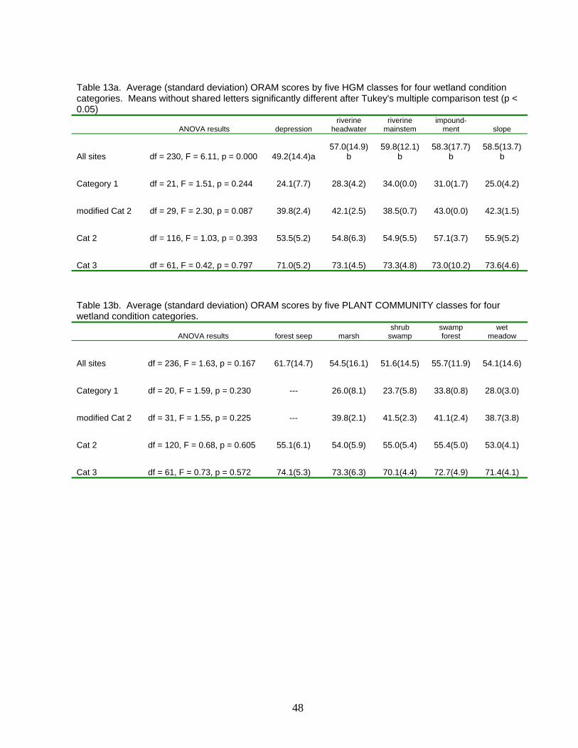
48

Table 13a. Average (standard deviation) ORAM scores by five HGM classes for four wetland condition categories. Means without shared letters significantly different after Tukey's multiple comparison test (p < 0.05)

ANOVA results

depression riverine

headwater riverine

mainstem impound-

ment

slope

All sites df = 230, F = 6.11, p = 0.000 49.2(14.4)a 57.0(14.9)

b 59.8(12.1)

b 58.3(17.7)

b 58.5(13.7)

b

Category 1 df = 21, F = 1.51, p = 0.244 24.1(7.7) 28.3(4.2) 34.0(0.0) 31.0(1.7) 25.0(4.2)

modified Cat 2 df = 29, F = 2.30, p = 0.087 39.8(2.4) 42.1(2.5) 38.5(0.7) 43.0(0.0) 42.3(1.5)

Cat 2 df = 116, F = 1.03, p = 0.393 53.5(5.2) 54.8(6.3) 54.9(5.5) 57.1(3.7) 55.9(5.2)

Cat 3 df = 61, F = 0.42, p = 0.797 71.0(5.2) 73.1(4.5) 73.3(4.8) 73.0(10.2) 73.6(4.6)

Table 13b. Average (standard deviation) ORAM scores by five PLANT COMMUNITY classes for four wetland condition categories.

ANOVA results

forest seep

marsh shrub

swamp swamp forest

wet meadow

All sites df = 236, F = 1.63, p = 0.167 61.7(14.7) 54.5(16.1) 51.6(14.5) 55.7(11.9) 54.1(14.6)

Category 1 df = 20, F = 1.59, p = 0.230 --- 26.0(8.1) 23.7(5.8) 33.8(0.8) 28.0(3.0)

modified Cat 2 df = 31, F = 1.55, p = 0.225 --- 39.8(2.1) 41.5(2.3) 41.1(2.4) 38.7(3.8)

Cat 2 df = 120, F = 0.68, p = 0.605 55.1(6.1) 54.0(5.9) 55.0(5.4) 55.4(5.0) 53.0(4.1)

Cat 3 df = 61, F = 0.73, p = 0.572 74.1(5.3) 73.3(6.3) 70.1(4.4) 72.7(4.9) 71.4(4.1)

49

Table 14. Average (standard deviation) number of hydrologic (Metric 3e), Habitat (Metric 4c) or combined stressors by wetland condition category. Means without shared letters significantly different (p <0.05) after Tukey's multiple comparison test.

Metric 3e Metric 4c Metric 3e + 4c

Category 1 2.0 (1.3)a 1.6(1.1)ab 3.6(1.7)a

mod Category 2 2.1(1.3)a 2.0(1.6)a 4.1(2.1)a

Category 2 1.2(1.3)b 1.1(1.4)b 2.4(2.2)b

Category 3 0.9(1.1)c 0.5(1.1)c 1.4(1.8)c

df 242 242 242

F statistic 8.54 10.27 14.25

p value 0.000 0.000 0.000

50

Table 15. Percentage of Metric 3e (Hydrologic alteration) stressors by condition category, county, TMDL region, HGM class, and plant community.

Condition category N ditchingtilingdikes weirsstormwater

input point

source filling roadsdredging other Category 1 22 27% 9% 9% 0% 36% 0% 50% 45% 5% 18% mod Category 2 32 53% 6% 16% 9% 9% 3% 38% 31% 13% 31% Category 2 124 31% 3% 10% 2% 2% 0% 18% 33% 4% 18% Category 3 65 11% 3% 8% 2% 3% 3% 18% 31% 2% 14% County CUYAHOGA 12 17% 8% 0% 8% 0% 0% 33% 33% 0% 25% GEAUGA 67 25% 3% 9% 1% 3% 1% 24% 36% 1% 28% PORTAGE 108 35% 5% 12% 3% 6% 2% 22% 33% 6% 12% SUMMIT 56 21% 4% 9% 4% 13% 0% 23% 30% 7% 18% TMDL region a Upper 94 33% 5% 12% 3% 10% 0% 18% 29% 3% 16% b Middle 77 27% 1% 4% 0% 6% 3% 31% 40% 6% 23% c Lower 45 27% 7% 13% 2% 4% 2% 24% 38% 7% 20% d Tinkers Creek 27 19% 4% 15% 11% 0% 0% 19% 22% 0% 11% HGM class depression 87 37% 8% 9% 2% 9% 1% 22% 28% 5% 15% fringing 9 22% 0% 22% 11% 0% 0% 11% 0% 0% 44% headwater 40 28% 3% 8% 0% 5% 0% 23% 30% 3% 20% impoundment 16 6% 0% 25% 0% 13% 0% 44% 63% 0% 13% mainstem 53 30% 4% 6% 4% 4% 2% 23% 47% 9% 21% slope 35 20% 0% 9% 6% 6% 3% 26% 29% 3% 20% Plant community forest seep 18 17% 0% 6% 0% 6% 6% 22% 28% 0% 17% marsh 85 31% 5% 13% 4% 8% 2% 22% 42% 4% 21% shrub swamp 42 24% 0% 12% 7% 7% 0% 21% 31% 10% 14% swamp forest 65 34% 6% 8% 2% 5% 0% 17% 20% 5% 15% wet meadow 27 26% 7% 4% 0% 7% 0% 44% 44% 4% 26%

51

Table 16. Percentage of Metric 4c (Habitat Alteration) stressors by condition category, county, TMDL region, HGM class, and plant community.

Condition class N mowing grazingclear-cuttin

select cutting

woody debris removal

sedi-mentation

toxic pollut.

shrub removal

aq bed removal farming

nutrient enrichment dredg-ing

Category 1 22 55% 14% 14% 9% 14% 14% 0% 9% 0% 14% 23% 5% mod Category 2 32 59% 3% 3% 19% 16% 16% 3% 25% 0% 16% 13% 9% Category 2 124 25% 2% 2% 19% 8% 9% 2% 10% 1% 10% 10% 7% Category 3 65 8% 3% 3% 5% 2% 8% 0% 3% 0% 6% 5% 5% County CUYAHOGA 12 25% 0% 0% 8% 0% 0% 0% 8% 0% 8% 0% 0% GEAUGA 67 21% 10% 10% 7% 4% 9% 0% 9% 0% 6% 12% 6% PORTAGE 108 31% 2% 2% 23% 9% 9% 0% 12% 1% 15% 10% 6% SUMMIT 56 30% 0% 0% 7% 11% 14% 5% 9% 0% 7% 11% 9% TMDL Region a Upper 94 32% 4% 4% 15% 5% 4% 1% 11% 0% 5% 4% 6% b Middle 77 25% 4% 4% 10% 12% 16% 1% 12% 1% 14% 18% 8% c Lower 45 29% 2% 2% 16% 9% 13% 2% 11% 0% 13% 11% 9% d Tinkers Creek 27 19% 4% 4% 22% 4% 7% 0% 4% 0% 11% 7% 0% HGM class depression 87 32% 1% 1% 20% 10% 8% 1% 11% 0% 13% 9% 6% fringing 9 22% 0% 0% 33% 11% 22% 0% 0% 11% 11% 33% 11% headwater 40 30% 5% 5% 15% 10% 8% 0% 20% 0% 5% 5% 5% impoundment 16 13% 6% 6% 13% 13% 19% 0% 0% 0% 13% 13% 0% mainstem 53 25% 6% 6% 11% 2% 9% 2% 4% 0% 11% 11% 9% slope 35 29% 6% 6% 3% 6% 11% 3% 14% 0% 9% 11% 9% Plant comm. forest seep 18 22% 0% 0% 11% 6% 11% 0% 11% 0% 11% 6% 11% marsh 85 24% 5% 5% 11% 7% 7% 0% 5% 1% 13% 13% 7% shrub swamp 42 31% 2% 2% 14% 10% 12% 2% 12% 0% 5% 12% 5% swamp forest 65 35% 2% 2% 26% 9% 8% 2% 14% 0% 9% 5% 6% wet meadow 27 22% 11% 11% 4% 4% 22% 4% 11% 0% 15% 19% 7%

52

Table 17. Average (standard deviation) number stressors and average Weighted Stressor Score from the PA Stressor checklist. Means without shared letters significantly different (p <0.05) after Tukey's multiple comparison test.

Condition category

Number of Stressors

Weighted Stressor Score

Category 1 5.2 (2.8)a 14.7(10.2)ab

mod Category 2 4.0(2.5)a 8.1(6.3)a

Category 2 2.7(2.1)b 5.6(4.9)b

Category 3 1.8(1.6)c 3.4(4.2)c

Table 18. Average values for wetland soil paramters. Total area of all wetlands where soil samples were collected, mean (standard deviation) soil nutrient levels and the resultant cumulative nutrient content (for upper 10cm of each wetland) as determined by multiplying areal nutrient content by wetland area and summing the results for the entire wetland population sampled in the watershed (note Mg = 106 g).

Wetland area or soil paramete

Mean for all

Wetlands, (g/m2)

Total for sampled population Area (Ha) 1174.35 (n=202)

Total phosphorus 122.39(59.30) 1,481.8 Mg Total nitrogen 636.74(323.18) 8,087.0 Mg Total carbon 9333.71(4963.69) 113,979.4 Mg

HCl-phosphorus 46.98(38.22) 751.9 Mg H2O-phosphorus 0.32(0.43) 3,765.2 kg

Nitrate-N 0.37(0.88) 2,939.9 kg Phosphorus-sorption 9630(4048) 100,829.6 Mg

53

Table 19. Average (standard deviation) ORAM scores (N = 232) by land use intensity categories for different buffer distances. Land use intensity categories defined by quadrisecting 95th percentile of LDI distribution for each buffer distance category. Means without shared letters significantly different (p <0.05) after Tukey's multiple comparison test. 100 m 250 m 500 m 1000 m 2000 m 4000 m

low 59.2 (12.9)a 59.6(13.3)a 60.8(12.9)a 61.6(13.5)a 60.6(12.6)a 54.3(5.3)ab

medium 54.6(14.6)ab 55.2(14.1)ab 56.2(14.0)ab 54.3(13.5)ab 56.8(14.2)a 59.1(14.3)a

high 47.3(13.2)bc 52.5(12.3)bc 50.6(13.1)bc 52.3(12.4)bc 55.6(13.3)a 53.9(14.0)b

very high 37.2(12.2)c 39.5(14.3)d 44.3(16.0)c 46.8(16.5)c 45.7(16.0)b 50.9(15.7)ab

df 3 3 3 3 3 3

F statistic 17.3 14.5 12.2 10.1 8.1 3.9

p value 0.000 0.000 0.000 0.000 0.000 0.011

Table 20. Agreement between LDI and ORAM assessments. Mean (standard deviation) of ORAM scores (N =232) by "agreement" categories for different buffer distances. Means without shared letters significantly different (p <0.05) after Tukey's multiple comparison test. "Under" by 1, 2, or 3 means the LDI predicted the wetland to be in worse condition than ORAM. "Over" by 1, 2, or 3 means the LDI predicted the wetland to be in better condition than ORAM. "Same category" means LDI and ORAM were in agreement. LDI land use intensity categories and ORAM equated as follows: low ~ Category 3, medium = Category 2, high ~ modified Category 2, very high ~ Category 1. 100 m 250 m 500 m 1000 m 2000 m 4000 m

under by 3 --- --- 67.8(1.9)ab 72.1(6.1)a 71.2(7.7)ab 72.2(6.0)a

under by 2 55.8(6.7)abc 61.0(10.2)ab 60.6(11.4)ad 59.1(9.0)ab 63.3(11.0)a 63.9(10.0)ab

under by 1 59.6(13.4)a 60.5(12.3)a 59.9(11.9)a 61.3(12.2)a 59.9(12.5)a 59.5(12.0)bc

same category 61.2(15.0)a 57.8(16.3)ab 57.6(16.2)ad 54.0(16.2)b 52.3(15.0)bc 47.1(11.8)d

over by 1 51.3(9.9)b 51.5(8.6)b 48.7(10.9)be 47.3(10.9)bc 45.5(10.5)c 37.8(11.1)e

over by 2 38.1(7.5)c 36.8(10.7)c 35.0(7.0)ce 35.2(3.3)c 30.6(6.6)cd 29.4(4.0)e

over by 3 31.9(2.3)cd 31.9(2.3)cd 31.5(2.1)cde 30.0 --- ---

df 5 5 6 6 5 5

F statistic 17.6 12.2 9.9 10.8 16.2 33.3

p value 0.000 0.000 0.000 0.000 0.000 0.000

54

Table 21. Agreement between LDI and VIBI. Mean (standard deviation) of VIBI scores by "agreement" categories for different buffer distances. Categories grouped into "under-categorized", "same category" and "over-categorized" due to small sample size of Level 3 data. Means without shared letters significantly different (p <0.05) after Tukey's multiple comparison test. "Unde-categorized" means the LDI predicted the wetland to be in worse condition than VIBI. "Over-categorized" means the LDI predicted the wetland to be in better condition than VIBI. "Same category" means LDI and VIBI were in agreement. LDI land use intensity categories and VIBI equated as follows: low ~ SWLH, medium = WLH, high ~ RWLH, very high ~ LQWLH. 100 m 250 m 500 m 1000 m 2000 m 4000 m

under-categorized 71.3(21.6)a 82.4(10.9)a 79.1(12.7)a 71.2(21.0)a 75.1(13.5)a 74.8(14.8)a

same category 77.1(11.3)a 69.0(11.6)a 57.7(10.0)ab 67.0(13.4)ab 72.5(26.2)a 75.0ab

over-categorized 53.9(22.0)b 46.1(15.2)b 44.2(17.4)b 39.7(6.4)b 38.0(9.6)b 38.0(9.5)b

df 2 2 2 2 2 2

F statistic 3.5 17.1 13.3 3.7 13.6 13.6

p value 0.051 0.000 0.000 0.044 0.000 0.000

N 21 21 21 21 21 21

55

Table 22. Agreement in condition category assignment between ORAM Antiegradation condition classes, PA Weighted Stressor Score condition classes and Wetland Tiered Aquatlc Life Uses (WTALU) categories for 22 Level 3 assessment sites.

Site site name ORAM Antideg

Category

PA Weighted Stressor

Score Stressor ClassVIBI

score WTALU

categories %agree ORAM-

PA %agree

WTALU-PA %agree ORAM-

WTALU 2001 Alexander Rd 48 Cat2 14 fair 60 WLH under by 1 under by 1 same category 2005 Old Forge Rd 74 Cat3 1 good 94 SWLH under by 1 under by 1 same category 2008 Bartholomew Rd 52 Cat2 18 fair 47 RWLH under by 1 same category over by 1 2013 Ward 62 Cat2 12 fair 50 RWLH under by 1 same category over by 1 2014 Brecksville 51 Cat2 21 fair 24 LQWLH under by 1 over by 1 over by 2 2015 Black Rd 40 mod Cat2 6 excellent 36 RWLH over by 2 over by 2 same category 2016 Wake Robin 74 Cat3 1 excellent 75 WLH same category over by 1 over by 1 2017 Quail Hollow 59 Cat2 1 good 50 RWLH same category over by 1 over by 1 2020 Thut 70 Cat3 0 excellent 84 SWLH same category same category same category 2023 Bath Rd 49 Cat2 1 good 36 RWLH same category over by 1 over by 1 2025 Rhinehart 65 Cat3 11 fair 74 SWLH under by 2 under by 2 same category 2027 Hasbrouck 77 Cat3 1 excellent 94 SWLH same category same category same category 2028 Bridge Creek 62 Cat2 3 good 47 RWLH same category over by 1 over by 1 2029 Twinsburg 70 Cat3 3 excellent 74 SWLH same category same category same category 2031 Miller 49.5 Cat2 8 poor 54 RWLH under by 1 same category over by 1 2032 Aquilla Rd 73 Cat3 3 good 84 SWLH under by 1 under by 1 same category 2033 Good Year 78 Cat3 9 good 84 SWLH under by 1 under by 1 same category 2034 Oak Knolls 71 Cat3 10 excellent 69 WLH same category over by 1 over by 1 2036 Tare Creek 74 Cat3 15 fair 80 SWLH under by 2 under by 2 same category 2037 Wingfoot Lake 50 Cat2 21 fair 53 WLH under by 1 under by 1 same category 2040 South Rider Rd 78 Cat3 4 good 91 SWLH under by 1 under by 1 same category 2042 Marsh Wetlands 75 Cat3 3 good 77 SWLH under by 1 under by 1 same category

under by 2 9.1% 9.1% 0.0% under by 1 50.0% 31.8% 0.0% same 36.4% 27.3% 59.1% over by 1 0.0% 27.3% 36.4% over by 2 4.5% 4.5% 4.5%

56

Table 23. Percentage of wetlands by condition category for LDI 100 m, LDI 200 m, ORAM, Weighted Stressor Score (PA WSS), and the VIBI. * n = 22 and VIBI distribution is truncated below the "fair" class.

LDI100 m

LDI250 m

ORAM

PA WSS

VIBI*

Poor 6.9 9.9 9.1 11.1 4.5

Fair 12.4 16.7 13.2 9.9 31.8

Good 22.7 29.2 51.0 23.5 18.2

Excellent 57.9 44.2 26.7 55.6 45.5

Table 24. ANOVA summary table for comparison of mean ORAM and VIBI scores from Ohio EPA's reference wetland dataset and results from Cuyahoga and Urban Wetland Study. Means without shared letters significantly different after Tukey's multiple comparison test (p < 0.05).

Antidegradation Categories

ORAM v. 5

WTALU categories

VIBI score

Category 1 26.0(6.1)a LQWLH 13.8(7.5)a

modified Cat 2 39.3(2.4)b RWLH 41.8(9.1)b

Category 2 55.8(5.2)c WLH 61.3(8.6)c

Category 3 74.8(6.5)d SWLH 78.4(11.1)d

Cuyahoga 55.5(14.4)c Cuyahoga 64.4(21.6)c

Urban 43.9(12.6)eb Urban 36.3(14.6)eb

--- --- Mitigation 30.0(14.1)eb

--- --- Bank 38.2(16.8)eb

df 5 df 6

F statistic 101.81 F statistic 126.36

p value 0.000 p value 0.000

N 468 N 297

57

Table 25. Summary statistics for ORAM scores based on first 50, 100, 125, 150, 200, and 243 points sampled.

Number of points sampled Mean st dev 95% CI

25th percentile median

75th percentile

50 points 60.2 13.7 3.8 50.0 60.3 73.3

100 points 56.8 15.4 3.0 45.0 55.5 71.8

125 points 55.6 15.5 2.7 44.0 54.5 69.3

150 points 55.0 15.4 2.5 44.8 53.5 66.1

200 points 55.4 14.7 2.0 46.6 54.8 66.4

243 points 55.1 14.6 1.8 46.5 54.5 66.0

58

Table 26. Descriptive statistics of wetland area by TMDL region and condition category. Number of Points Sampled

Condition Category

mean

st dev

95% CI

N

% of total resource

1st 50 points Cat 1 32.5 2.1 2.9 2 4%

mod Cat 2 39.3 2.6 2.3 5 10%

Cat 2 55.1 5.3 2.2 23 46%

Cat 3 74.0 4.5 2.0 20 40%

1st 100 points Cat 1 27.3 6.2 4.9 6 6%

mod Cat 2 40.4 2.3 1.0 19 19%

Cat 2 54.2 4.9 1.5 41 41%

Cat 3 74.3 5.8 1.9 34 34%

1st 125 points Cat 1 28.3 6.4 3.6 12 10%

mod Cat 2 40.5 2.6 1.0 20 16%

Cat 2 54.3 5.4 1.3 55 44%

Cat 3 74.1 5.6 1.9 38 30%

1st 150 points Cat 1 27.0 6.6 3.3 15 10%

mod Cat 2 40.6 2.3 0.9 22 15%

Cat 2 54.0 5.2 1.2 70 47%

Cat 3 73.7 5.9 1.8 43 29%

1st 200 points Cat 1 26.5 6.8 3.2 17 9%

mod Cat 2 40.5 2.6 1.0 27 14%

Cat 2 54.4 5.4 1.1 99 50%

Cat 3 72.8 5.6 1.5 57 29%

All 243 points Cat 1 26.6 6.8 2.8 22 9%

mod Cat 2 2.5 2.5 0.9 31 13%

Cat 2 5.4 5.4 1.0 123 51%

Cat 3 5.5 5.5 1.3 64 26%

59

Table 27. Summary of staffing scenarios to achieve full rotating basin wetland monitoring and assessment by 2013 with Level 3 sampling for ONE indicator taxa group. Numbers should be doubled for each additional taxa group.

work load

year(s)

Scenario 1:

NOMINAL +0 FTEs

Scenario 2:

MINIMAL +2 FTEs

Scenario 3:

PARTIAL +4 FTEs

Scenario 4:

FULL +6 FTEs

Continue current WPD grant commitments

2007-2009 YES YES YES YES

Maintain 2007 Levels of 401 Program Technical Support: enforcement, litigation, MBRT reviews, permit reviews, WRRSP, ORAM reviews, Mitigation review, Rule Development, etc.)

2007+ NO YES YES YES

Maintain 2007 Levels of ORAM and IBI Training

2007+ NO YES YES YES

Pilot Integrated Wetland-Stream Assessment Project

2009-2010 YES YES YES YES

Expanded Mitigation Assessment (Monitor 5-10% of "open" projects per year)

2008+ NO YES YES YES

Number of New WPD Research Projects

2010, 2012 2 2 2 2

Degree to which full statewide monitoring and assessment can be achieved by 2013

2011+ NOMINAL 5 HUC11

every other year

MINIMAL 5 HUC11 each year

PARTIAL 10-15

HUC11 each year

FULL 25

HUC11 each year

TOTAL FTEs

2 4 6 8

60

Figure 1. Ecoregions of the Cuyahoga Watershed and surrounding areas. Subregion 61a = Erie Lake Plain, 61b = Mosquito Creek/Pymatuning Lowlands, 61c = Low Lime Drift Plain, 61d = Erie Gorges, 61e = Summit Interlobate Area.

61

Figure 2. Upper Cuyahoga River Map and Attainment Status as of 2003. From Total Maximum Daily Loads for the Upper Cuyahoga River Final Report September 2004.

62

Figure 3. Schematic representation of Upper Cuyahoga River Watershed. From Total Maximum Daily Loads for the Upper Cuyahoga River Final Report September 2004.

63

Figure 4. Land use/land cover of Upper Cuyahoga River Basin. From Total Maximum Daily Loads for the Upper Cuyahoga River Final Report September 2004.

64

Figure 5. Middle Cuyahoga River. From Total Maximum Daily Loads for the Middle Cuyahoga River Final Report March 2000.

65

Figure 6. Schematic representation of Middle Cuyahoga River watershed. From Total Maximum Daily Loads for the Middle Cuyahoga River Final Report March 2000.

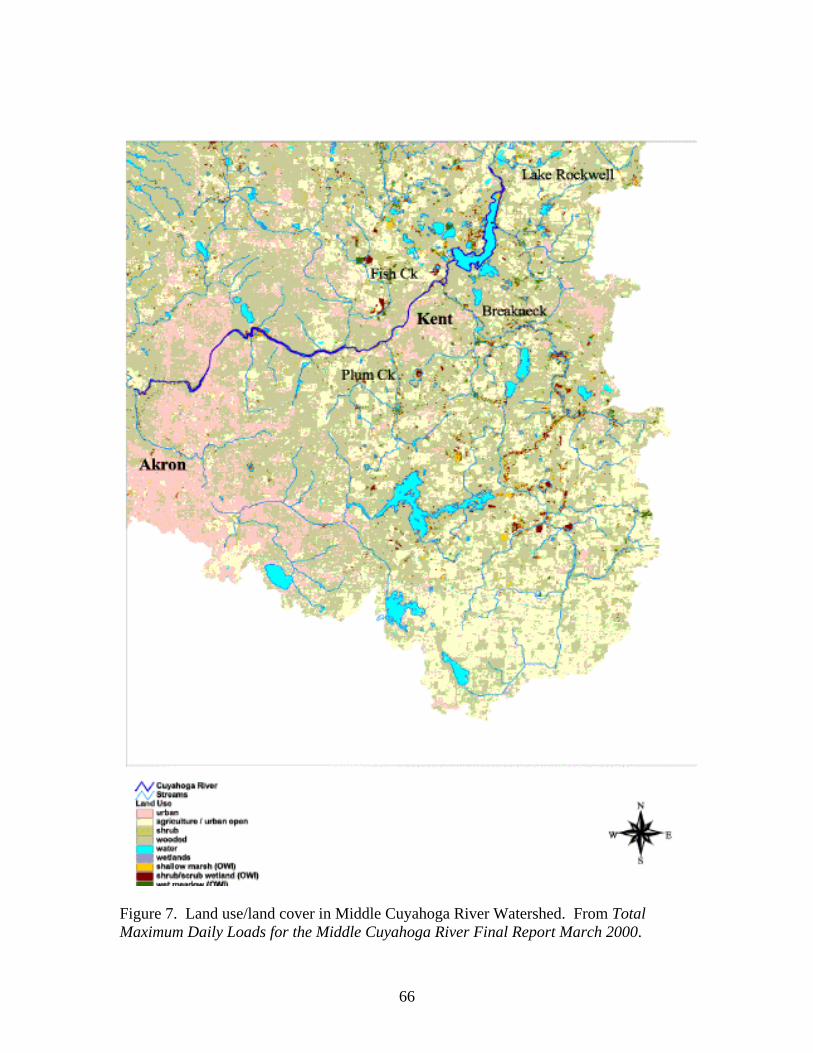
66

Figure 7. Land use/land cover in Middle Cuyahoga River Watershed. From Total Maximum Daily Loads for the Middle Cuyahoga River Final Report March 2000.

67

Figure 8. Lower Cuyahoga River Watershed. From Total Maximum Daily Loads for the Lower Cuyahoga River Final Report September 2003.

68

Figure 9a. Schematic representation of the Lower Cuyahoga River Watershed. From Total Maximum Daily Loads for the Lower Cuyahoga River Final Report September 2003.

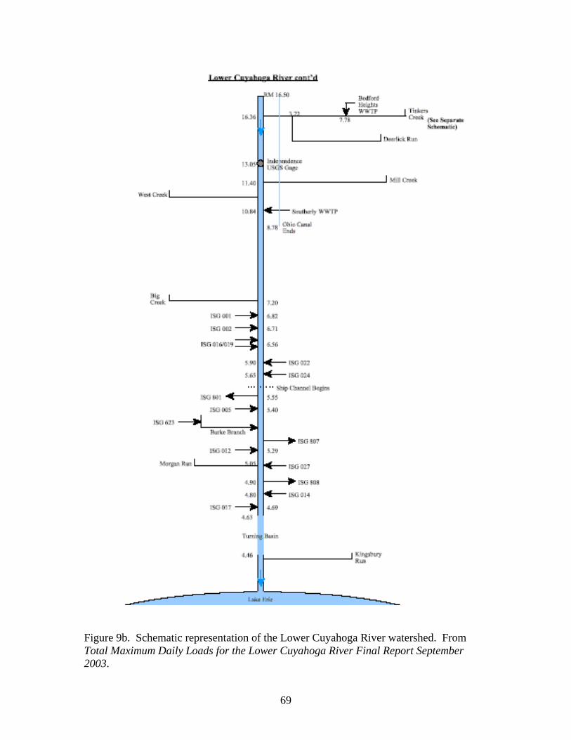
69

Figure 9b. Schematic representation of the Lower Cuyahoga River watershed. From Total Maximum Daily Loads for the Lower Cuyahoga River Final Report September 2003.

70

Figure 9c. Schematic representation of Tinkers Creek portion of Lower Cuyahoga River watershed. From Total Maximum Daily Loads for the Lower Cuyahoga River Final Report September 2003.

71

Figure 10. Land use/land cover in the Lower Cuyahoga River watershed. From Total Maximum Daily Loads for the Lower Cuyahoga River Final Report September 2003.

72

Figure 11. GRTS map showing the four hundred initial sampling points in the CRW of which 242 wetlands were evaluated (Mack and Fennessy 2005).

73

Figure 12. Preliminary examination of sample points was done using digital aerial photos, supplied by Cuyahoga, Summit, Portage and Geauga counties. These images had a one-meter ground resolution and were orthorectified. Each sample location was plotted on the airphoto and the land use at that point examined. Points were excluded from further consideration if it was clear that a wetland no longer existed at that point.

74

Figure 13. The fate of wetland points included in this study, including wetlands sampled using ORAM (n = 242) and level 3 techniques (n = 26), duplicate points (more than one sampling point was dropped in a single wetland assessment area, n = 18), access to the site was denied by landowners (n = 45), and no wetland was at the point or within 60 m of it and this was due to mapping errors in the OWI (n = 38), filling/conversion of a mapped wetland (n = 8), or the cause was unable to be determined (n = 15).

Figure 14. The distribution of wetlands over the seven HGM classes (sensu Brinson 1993).

10.4%

4.1%

2.2%

12.3%

4.9%

66.1%Wetlands Assessed

No Wetland Found - Mapping Error

Access Denied

Duplicate Point

No Wetland Found - Undetermined

No Wetland Found - Filled/Converted

depression37%

riverine mainstem20%

riverine headwater16%

slope15%

impoundment7%

fringing4%

bog1%

75

Figure 15. Plot showing all sites sampled ordered by ORAM score. The ORAM scoring range is 0 to 100; sites sampled in this probabilistic design ranged from scores of 16 to 94.

0

10

20

30

40

50

60

<0.04 0.04 to <0.12 0.12 to <1.2 1.2 to <4 4 to <10.1 10.1 to <20.2 >20.2Size (ha)

Porp

ortio

n W

etla

nds

DepressionalImpoundmentsRiverineSlope

Figure 16. The size distribution of wetlands within major HGM classes. Note the large percentage of all wetlands within the size category 0.12 to <1.2 ha.

0 30 60 90 120 150 180 210 240 270

10

20

30

40

50

60

70

80

90

100

site rank

OR

AM s

core

76

Figure 17. Scatterplots of LDI score calculated from Minnesota coefficients (LDI-MN) and LDI score calculated from Florida coefficients (LDI-FL) for different buffer distances (100 m, 250 m, 500 m, 1000 m, 2000 m, 4000 m). All R2 > 96.9% and p < 0.001.

c. 500 meters f. 4000 meters

b. 250 meters e. 2000 meters

a. 100 meters d. 1000 meters

0 100 200 300 400

100

200

300

400

500

600

700

800

LDI-MN100m

LDI-F

L100

m

0 100 200 300 400

100

200

300

400

500

600

700

800

LDI-MN250m

LDI-F

L250

m

0 100 200 300 400

100

200

300

400

500

600

700

800

LDI-MN500

LDI-F

L500

0 100 200 300 400

100

200

300

400

500

600

700

LDI-MN1000

LDI-F

L100

0

0 50 100 150 200 250 300 350

100

200

300

400

500

600

700

LDI-MN2000

LDI-F

L200

0

0 50 100 150 200 250 300 350

100

200

300

400

500

600

700

LDI-MN4000

LDI-F

L400

0

77

Figure 18. Box and whisker plots of mean (standard deviation) LDI scores (using Minnesota coefficients) for each buffer distance (n = 233, df = 5, F = 38.01, p = 0.000).

100m 250m 500m 1000m 2000m 4000m

0

100

200

300

400

70.4 (83.3) 97.3(85.2) 114.8(81.5) 130.5(73.5) 141.4(65.3) 152.0(55.5)

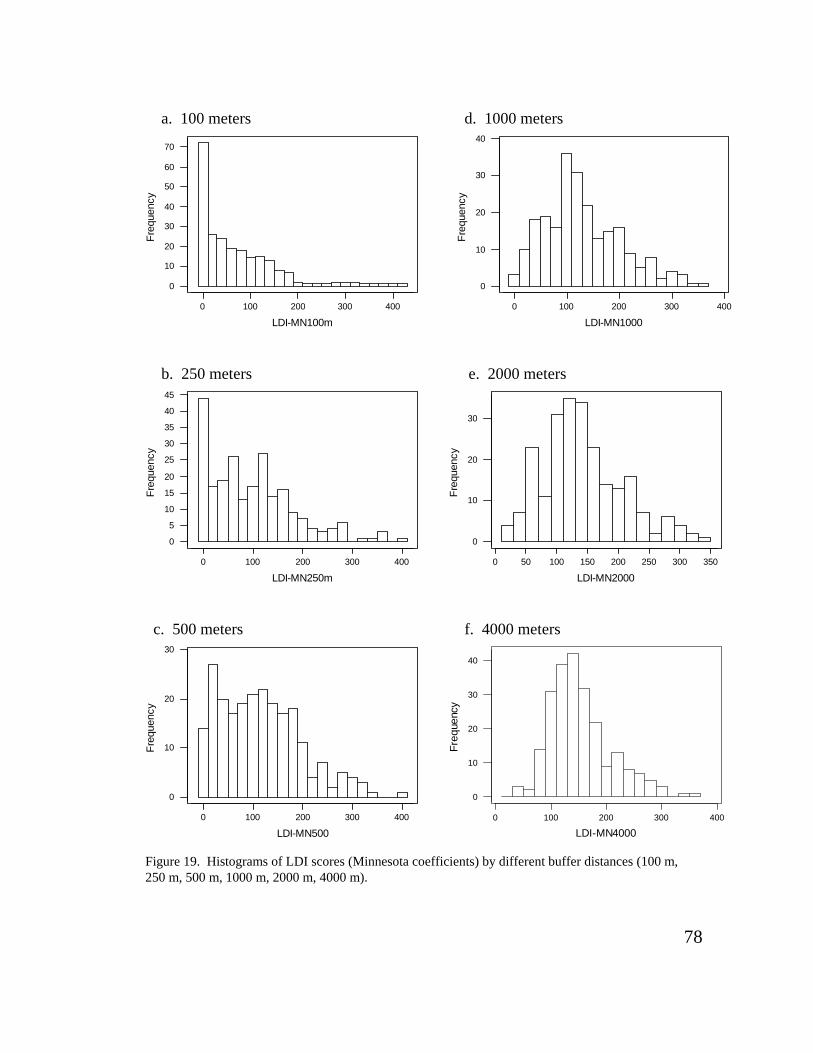
78

Figure 19. Histograms of LDI scores (Minnesota coefficients) by different buffer distances (100 m, 250 m, 500 m, 1000 m, 2000 m, 4000 m).

c. 500 meters f. 4000 meters

b. 250 meters e. 2000 meters

a. 100 meters d. 1000 meters

0 100 200 300 400

0

10

20

30

40

50

60

70

LDI-MN100m

Freq

uenc

y

0 100 200 300 400

0

5

10

15

20

25

30

35

40

45

LDI-MN250m

Freq

uenc

y

0 100 200 300 400

0

10

20

30

LDI-MN500

Freq

uenc

y

0 100 200 300 400

0

10

20

30

40

LDI-MN1000

Freq

uenc

y

0 50 100 150 200 250 300 350

0

10

20

30

LDI-MN2000

Freq

uenc

y

0 100 200 300 400

0

10

20

30

40

LDI-MN4000

Freq

uenc

y

79

Figure 20. Scatterplots (and regression line) of LDI scores (Minnesota coefficients) and ORAM scores (df = 232, p < 0.001).

c. 500 meters (R2 = 15.8%) f. 4000 meters (R2 = 4.8%)

b. 250 meters (R2 = 16.7%) e. 2000 meters (R2 = 6.6%)

a. 100 m (R2 = 16.9%) d. 1000 meters (R2 = 12.4%)

4003002001000

100

90

80

70

60

50

40

30

20

10

LDI-MN100

OR

AM

sco

re

4003002001000

100

90

80

70

60

50

40

30

20

10

LDI-MN250

OR

AM

sco

re

4003002001000

100

90

80

70

60

50

40

30

20

10

LDI-MN500

OR

AM s

core

4003002001000

100

90

80

70

60

50

40

30

20

10

LDI-MN1000

OR

AM

sco

re

350300250200150100500

100

90

80

70

60

50

40

30

20

10

LDI-MN2000

OR

AM s

core

350300250200150100500

100

90

80

70

60

50

40

30

20

10

LDI-MN4000

OR

AM

sco

re

80

Figure 21. Box and whisker plots of LDI scores (Minnesota coefficients) for different wetland condition categories at different buffer distances (100 m, 250 m, 500 m, 1000 m, 2000 m, 4000 m).

a. 100 meters d. 1000 meters

c. 500 meters f. 4000 meters

b. 250 meters e. 2000 meters

Cat1 Cat2 mod Cat2 Cat3

0

100

200

300

400

LDI-M

N10

0

Cat1 Cat2 mod Cat2 Cat3

0

100

200

300

400

LDI-M

N10

00

Cat1 Cat2 mod Cat2 Cat3

0

100

200

300

400

LDI-M

N25

0

Cat1 Cat2 mod Cat2 Cat3

0

50

100

150

200

250

300

350

LDI-M

N20

00

Cat1 Cat2 mod Cat2 Cat3

0

100

200

300

400

LDI-M

N50

0

Cat1 Cat2 mod Cat2 Cat3

0

50

100

150

200

250

300

350

LDI-M

N40

00

81

0

20

40

60

80

100

120

140

160

180

200

100 250 500 1000 2000 4000

Buffer Distance (m)

LDI S

core

DepressionalImpoundmentsRiverineSlope

A

B

C C

A

B

C C

A

B

C C

A

AC

B

BC

AA

B

C

A

AB

B

B

Figure 22. Mean LDI scores (using Minnesota coefficients) for each buffer distance stratified by HGM class. Different letters indicate statistically significant differences between HGM classes for that buffer distance (letters indicate significant differences for different HGM classes for each buffer distance). Error bars are the standard error of the mean (ANOVA, 100 m: F=5.17, p=0.002; 250 m: F=6.14, p=0.001; 500 m: F=5.65, p=0.001; 1000 m: F=5.55, p=0.001; 2000 m: F=5.09, p=0.002; 4000 m: F=4.28, p=0.006.

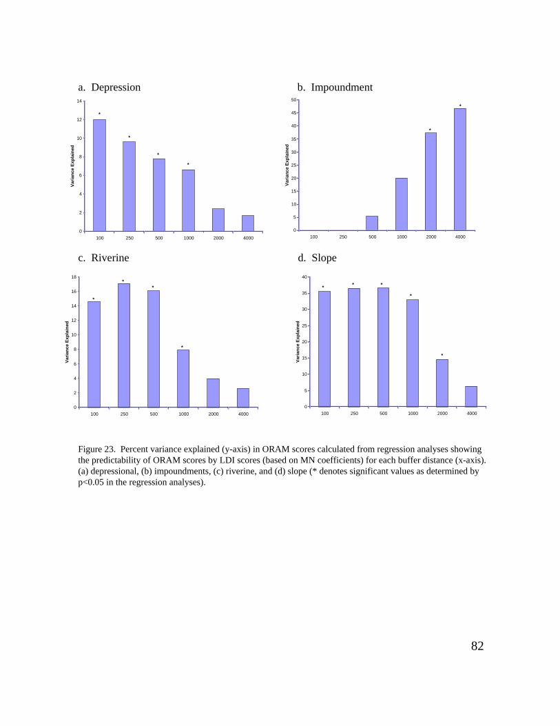
82

a. Depression b. Impoundment

c. Riverine d. Slope

0

2

4

6

8

10

12

14

100 250 500 1000 2000 4000

Varia

nce

Expl

aine

d

*

*

*

*

0

5

10

15

20

25

30

35

40

45

50

100 250 500 1000 2000 4000

Varia

nce

Expl

aine

d

*

*

0

2

4

6

8

10

12

14

16

18

100 250 500 1000 2000 4000

Varia

nce

Expl

aine

d

*

**

*

0

5

10

15

20

25

30

35

40

100 250 500 1000 2000 4000

Varia

nce

Expl

aine

d

* * *

*

*

Figure 23. Percent variance explained (y-axis) in ORAM scores calculated from regression analyses showingthe predictability of ORAM scores by LDI scores (based on MN coefficients) for each buffer distance (x-axis). (a) depressional, (b) impoundments, (c) riverine, and (d) slope (* denotes significant values as determined by p<0.05 in the regression analyses).

83

a. Depression b. Impoundment

c. Riverine d. Slope

Figure 24A. Percent variance explained in ORAM scores (y-axis) calculated from regression analyses showing the predictability of ORAM scores by LDI score (FL coefficients) for each buffer distance (x-axis). (a) depressional, (b) impoundments, (c) riverine, (d) slope (* denotes significant values as determined by p<0.05 from analyses of variance).

0

2

4

6

8

10

12

100 250 500 1000 2000 4000

Buffer Distance (m)

% V

ari

an

ce E

xp

lain

ed

*

*

* *

0

5

10

15

20

25

30

35

40

45

50

100 250 500 1000 2000 4000

Buffer Distance (m)

% V

ari

an

ce E

xp

lain

ed

**

0

2

4

6

8

10

12

14

16

18

100 250 500 1000 2000 4000

Buffer Distance (m)

% V

ari

an

ce E

xp

lain

ed

*

*

*

*

0

5

10

15

20

25

30

35

40

100 250 500 1000 2000 4000

Buffer Distance (m)

% V

ari

an

ce E

xp

lain

ed

** *

*

*

84

a. Depression b. Impoundment

c. Riverine d. Slope

Figure 24B. Percent variance explained in ORAM scores (y-axis) calculated from regression analyses showing the predictability of ORAM scores by the proportion of forest in each buffer distance (x-axis). (a) depressional, (b) impoundments, (c) riverine, (d) slope (* denotes significant values as determined by p<0.05 from analyses of variance).

0

1

2

3

4

5

6

100 250 500 1000 2000 4000

Buffer Distance (m)

% V

ari

an

ce E

xp

lain

ed

**

0

5

10

15

20

25

30

100 250 500 1000 2000 4000

Buffer Distance (m)

% V

ari

an

ce E

xp

lain

ed

*

0

0.5

1

1.5

2

2.5

3

100 250 500 1000 2000 4000

Buffer Distance (m)

% V

ari

an

ce E

xp

lain

ed

0

1

2

3

4

5

6

7

100 250 500 1000 2000 4000

Buffer Distance (m)

% V

ari

an

ce E

xp

lain

ed

85

a. Depression b. Impoundment

c. Riverine d. Slope

Figure 24C. Percent variance explained in ORAM scores (y-axis) calculated from regression analyses showing the predictability of ORAM scores by the proportion of agricultural/pastoral land in each buffer distance (x-axis). (a) depressional, (b) impoundments, (c) riverine, (d) slope (* denotes significant values as determined by p<0.05 from analyses of variance).

0

0.5

1

1.5

2

2.5

3

3.5

4

4.5

5

100 250 500 1000 2000 4000

Buffer Distance (m)

% V

ari

an

ce E

xp

lain

ed

*

0

1

2

3

4

5

6

7

8

9

10

100 250 500 1000 2000 4000

Buffer Distance (m)

% V

ari

an

ce E

xp

lain

ed

0

2

4

6

8

10

12

14

100 250 500 1000 2000 4000

Buffer Distance (m)

% V

ari

an

ce E

xp

lain

ed

*

*

*

0

1

2

3

4

5

6

7

8

100 250 500 1000 2000 4000

Buffer Distance (m)

% V

ari

an

ce E

xp

lain

ed

86

a. Depression b. Impoundment

c. Riverine d. Slope

Figure 24D. Percent variance explained in ORAM scores (y-axis) calculated from regression analyses showing the predictability of ORAM scores by the proportion of urban/residential land in each buffer distance (x-axis). (a) depressional, (b) impoundments – note the change from a positive slope to negative slope at 1000 m, (c) riverine, (d) slope (* denotes significant values as determined by p<0.05 from analyses of variance).

0

1

2

3

4

5

6

100 250 500 1000 2000 4000

Buffer Distance (m)

% V

ari

an

ce E

xp

lain

ed

*

0

5

10

15

20

25

30

100 250 500 1000 2000 4000

Buffer Distance (m)

% V

ari

an

ce E

xp

lain

ed

*+

+

-

-

-

0

0.5

1

1.5

2

2.5

3

3.5

4

4.5

100 250 500 1000 2000 4000

Buffer Distance (m)

% V

ari

an

ce E

xp

lain

ed

0

5

10

15

20

25

30

100 250 500 1000 2000 4000

Buffer Distance (m)

% V

ari

an

ce E

xp

lain

ed

*

* *

* *

87

Figure 25. Pie charts of LDI scores (Minnesota coefficients) for different buffer distances (100 m, 250 m, 500 m, 1000 m, 2000 m, 4000 m). “Low”, “medium”, “high”, and “very high” refer to the intensity of the land uses within the buffer distance. Low = 0-99, medium = 100-199, high = 200-299, very high = 300+.

a. 100 meters d. 1000 meters

c. 500 meters f. 4000 meters

b. 250 meters e. 2000 meters

high ( 29, 12.4%)

very high ( 16, 6.9%)

medium ( 53, 22.7%)

low (135, 57.9%)

low (49, 21.0%)

very high (42, 18.0%)

high (53, 22.7%)

medium (89, 38.2%)

low (103, 44.2%)

high ( 39, 16.7%)

very high ( 23, 9.9%)

medium ( 68, 29.2%)

low (79, 33.9%)

high (52, 22.3%)

very high (27, 11.6%)

medium (75, 32.2%)

low (34, 14.6%)

very high (39, 16.7%)

high (71, 30.5%)

medium (89, 38.2%)

low ( 4, 1.7%)

medium (83, 35.6%)

very high (47, 20.2%)high (99, 42.5%)

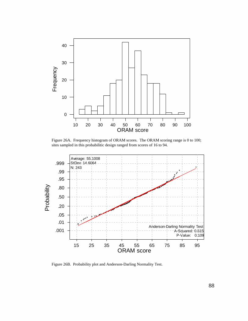
88

Figure 26A. Frequency histogram of ORAM scores. The ORAM scoring range is 0 to 100; sites sampled in this probabilitic design ranged from scores of 16 to 94.

Figure 26B. Probability plot and Anderson-Darling Normality Test.

10 20 30 40 50 60 70 80 90 100

0

10

20

30

40

ORAM score

Freq

uenc

y

Average: 55.1008StDev: 14.6064N: 243

Anderson-Darling Normality TestA-Squared: 0.615

P-Value: 0.109

15 25 35 45 55 65 75 85 95

.001

.01

.05

.20

.50

.80

.95

.99

.999

Prob

abilit

y

ORAM score

89

Figure 27A. The distribution of individual wetlands across the wetland category scheme (n=243).

Cat2 modified ( 32, 13.2%)

Cat1 ( 22, 9.1%)

Cat2 (124, 51.0%)

Cat3 ( 65, 26.7%)

Figure 27B. The distribution of acreage of wetlands (acres) across the wetland category scheme (n=243).

Cat1 ( 116, 3.0%

Cat2a ( 233, 6.1%)

Cat3 (2142, 55.7%)

Cat2b (1355, 35.2%)

90

Figure 28. Pie charts of percentage of wetlands (a, b, c, d) and acreage of wetlands (d, e, f, g) by four counties and four antidegradation condition categories: Cat1 = Category 2, Cat 2a = modified Category 2, Cat2b = Category 2, Cat3 = Category 3.

a. Geauga (number) e. Geauga (acreage)

Cat2a ( 7, 10.4%)

Cat1 ( 4, 6.0%)

Cat3 (33, 49.3%)

Cat2b (23, 34.3%)

Cat2a (15, 13.9%)

Cat1 (11, 10.2%)

Cat3 (20, 18.5%)

Cat2b (62, 57.4%)

b. Portage (number) f. Portage (acreage)

c. Summit (number) g. Summit (acreage)Cat2a ( 8, 14.3%)

Cat1 ( 6, 10.7%)

Cat3 (11, 19.6%)

Cat2b (31, 55.4%)

d. Cuyahoga (number) h. Cuyahoga (acreage)

Cat1 (1, 8.3%)

Cat2a (2, 16.7%)

Cat3 (1, 8.3%)

Cat2b (8, 66.7%)

Cat1 ( 11, 0.6%)Cat2a ( 53, 3.0%)

Cat2b ( 222, 12.5%)

Cat3 (1494, 83.9%)

Cat2a ( 65, 9.2%)

Cat1 ( 13, 1.8%)

Cat3 (226, 32.3%)

Cat2b (397, 56.7%)

Cat2a (108, 8.5%)

Cat1 ( 92, 7.2%)

Cat3 (408, 32.1%)

Cat2b (664, 52.2%)

Cat2a ( 8, 8.3%)

Cat1 ( 1, 0.7%)

Cat3 (13, 14.5%)

Cat2b (71, 76.5%)

91

Figure 29. Pie charts of percentage of wetlands (a, b, c, d) and acreage of wetlands (d, e, f, g) by TMDL report region and four antidegradation condition categories: Cat1 = Category 2, Cat 2a = modified Category 2, Cat2b = Category 2, Cat3 = Category 3.

a. Upper Cuyahoga (number) e. Upper Cuyahoga (acreage)

b. Middle Cuyahoga (number) f. Middle Cuyahoga (acreage)

c. Tinkers Creek (number) g. Tinkers Creek (acreage)

d. Lower Cuyahoga (number) h. Lower Cuyahoga (acreage)

Cat1 (11, 11.7%)

Cat2a (10, 10.6%)

Cat3 (17, 18.1%)

Cat2b (56, 59.6%)

Cat1 ( 3, 3.9%)

Cat2a (11, 14.3%)

Cat3 (33, 42.9%)

Cat2b (30, 39.0%)

Cat1 ( 4, 14.8%)

Cat2a ( 2, 7.4%)

Cat3 ( 4, 14.8%)

Cat2b (17, 63.0%)

Cat1 ( 4, 8.9%)

Cat2a ( 9, 20.0%)

Cat3 (11, 24.4%)

Cat2b (21, 46.7%)

Cat2a ( 17, 2.1%)Cat1 ( 19, 2.4%)

Cat3 (235, 29.8%)

Cat2b (517, 65.7%)

Cat2b ( 506, 24.7%)

Cat2a ( 106, 5.2%)

Cat1 ( 12, 0.6%)

Cat3 (1424, 69.5%)

Cat1 ( 4, 1.9%)

Cat2a (38, 18.1%)

Cat3 (69, 32.9%)

Cat2b (98, 47.1%)

Cat2a ( 72, 9.1%)

Cat1 ( 81, 10.2%)

Cat3 (414, 51.7%)

Cat2b (233, 29.1%)

92

Figure 30. Pie charts of percentage of wetlands (a, b, c, d) and acreage of wetlands (d, e, f, g) by HGM Class and four antidegradation condition categories: Cat1 = Category 2, Cat 2a = modified Category 2, Cat2b = Category 2, Cat3 = Category 3.

a. Depression (number) e. Depression (acreage)

b. Riverine (number) f. Riverine (acreage)

c. Slope (number) g. Slope (acreage)

d. Impoundment (number) h. Impoundment (acreage)

Cat1 (12, 13.8%)

Cat2a (17, 19.5%)

Cat3 (12, 13.8%)

Cat2b (46, 52.9%)

Cat1 ( 28, 4.3%)

Cat2a (167, 25.1%)

Cat3 (114, 17.2%)Cat2b (355, 53.4%)

Cat1 ( 5, 5.4%)

Cat2a ( 9, 9.7%)

Cat3 (32, 34.4%)

Cat2b (47, 50.5%)

Cat1 ( 83, 3.4%)

Cat2a ( 43, 1.8%)

Cat2b ( 830, 34.1%)

Cat3 (1478, 60.7%)

Cat1 ( 2, 5.7%)

Cat2a ( 3, 8.6%)

Cat3 (11, 31.4%)

Cat2b (19, 54.3%)

Cat1 ( 2, 0.4%)Cat2a ( 18, 3.8%)

Cat2b (110, 23.1%)

Cat3 (346, 72.7%)

Cat1 (3, 18.8%)

Cat2a (1, 6.2%)

Cat3 (7, 43.7%)

Cat2b (5, 31.2%)

Cat1 ( 3, 1.6%)Cat2a ( 2, 1.2%)

Cat2b ( 30, 17.8%)

Cat3 (131, 79.4%)

93

Figure 31A. Frequency histogram of number of stressors from the PA Stressor Checklist. The scoring range is 0 to 54; sites sampled in this probabilitic design ranged from scores of 0 to 11.

Figure 31B. Frequency histogram of Weighted Stressor Score derived from the PA Stressor Checklist. The scoring range is 0 to ~50; sites sampled in this probabilistic design ranged from scores of 0 to 40.

0 5 10

0

10

20

30

40

50

Number of Stressors

Freq

uenc

y

0 10 20 30 40

0

10

20

30

40

50

60

Weighted Stressor Score

Freq

uenc

y

94

Figure 32A. Box and whisker plots of number of stressors by wetland condition category. All means significantly different except Category 1 and modified Category 2 (df = 242, F = 17.91, p = 0.000).

Figure 32B. Box and whisker plots of weighted stressor score by wetland condition category. All means significantly different except modified Category 2 and Category and Category 2 and Category 3 (df = 242, F = 24.07, p = 0.000).

Category 1Category 2modif ied Category 2 Category 3

0

10

20

30

40

PA

Wei

ghte

d S

tress

or S

core

Category 1 modifiedCategory 2

Category 2 Category 3

0

5

10

Num

ber o

f PA

Che

cklis

t Stre

ssor

s

95

Figure 33A. Percentage of wetlands in poor, fair, good, and excellent condition as determined by the number of stressors from from the PA Stressor Checklist.

Figure 33B. Percentage of wetlands in poor, fair, good, and excellent condition as determined by the Weighted Stressor Score derived from the PA Stressor Checklist.

fair ( 29, 11.9%)

poor ( 21, 8.6%)

good ( 66, 27.2%)

excellent (127, 52.3%)

poor ( 27, 11.1%

fair ( 24, 9.9%)good ( 57, 23.5%)

excellent (135, 55.6%)

96

Figure 34A. Scatterplot of No. of Stressors and ORAM score. Horizontal solid lines areOhio wetland condition categories (see text). Vertical dashed lines represent quartiles of 95th

percentile of no. of stressor: poor (>6.0), fair(4.1-6.0), good (2.1-4.0), and excellent (0-2.0) (df = 242, R2 = 19.3%, F = 57.8, p = 0.000).

Figure 34B. Scatterplot of PA Weighted Stressor Score and ORAM score. Horizontal solid lines are Ohio wetland condition categories (see text). Vertical dashed lines represent quartiles of 95th percentile of stressor scores: poor (>17), fair(12-17), good (6-12), and excellent (0-6) (df = 242, R2 = 21.7%, F = 66.8, p = 0.000).

0 5 10

10

20

30

40

50

60

70

80

90

100

No. Stressors

OR

AM s

core

0 10 20 30 40

10

20

30

40

50

60

70

80

90

100

PA Weighted Stressor Score

OR

AM s

core

97

Figure 35. Percentage of wetlands in LQWLH (poor), RWLH (fair), WLH (good), and SWLH (excellent) condition as determined by Vegetation IBI scores. LQWLH = limited quality wetland habitat, RWLH = restorable wetland habitat, WLH = wetland habitat, SWLH = superior wetland habitat.

WLH ( 4, 18.2%)

LQWLH ( 1, 4.5%)

RWLH ( 7, 31.8%)

SWLH (10, 45.5%)

SWLH WLH RWLH LQWLH

25 35 45 55 65 75 85

0

10

20

30

40

50

60

70

80

90

100

ORAM Score

VIBI

sco

re

Figure 36. Scatterplot of VIBI score versus ORAM score. Line is regression line (df = 21, F = 63.7, R2 = 76.1%, p = 0.000.

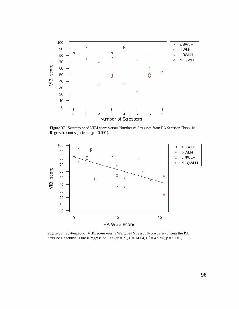
98

Figure 37. Scatterplot of VIBI score versus Number of Stressors from PA Stressor Checklist. Regression not signficant (p = 0.091).

Figure 38. Scatterplot of VIBI score versus Weighted Stressor Score derived from the PA Stressor Checklist. Line is regression line (df = 21, F = 14.64, R2 = 42.3%, p = 0.001).

a SWLH b WLH c RWLH d LQWLH

76543210

100

90

80

70

60

50

40

30

20

10

0

Number of Stressors

VIBI

sco

re

a SWLH b WLH c RWLH d LQWLH

0 10 20

0

10

20

30

40

50

60

70

80

90

100

PA WSS score

VIBI

sco

re

99

Figure 39. Scatterplots (and regression line) of LDI scores (Minnesota coefficients) and VIBI scores scores (df = 20).

c. 500 meters (R2 = 13.7%, p = 0.098) f. 4000 meters (R2 = 4.1%, p = 0.378)

b. 250 meters (R2 = 18.6%, p = 0.051) e. 2000 meters (R2 = 13.9%, p = 0.096)

a. 100 m (R2 = 13.3%, p =0.103) d. 1000 meters (R2 = 12.8%, p = 0.111)

a SWLH b WLH c RWLH d LQWLH

150100500

100

90

80

70

60

50

40

30

20

10

0

LDI-MN100

VIBI

sco

re

a SWLH b WLH c RWLH d LQWLH

2001000

100

90

80

70

60

50

40

30

20

10

0

LDI-MN1000

VIBI

sco

re

a SWLH b WLH c RWLH d LQWLH

2001000

100

90

80

70

60

50

40

30

20

10

0

LDI-MN250

VIBI

sco

re

a SWLH b WLH c RWLH d LQWLH

2001000

100

90

80

70

60

50

40

30

20

10

0

LDI-MN2000

VIBI

sco

re

a SWLH b WLH c RWLH d LQWLH

2001000

100

90

80

70

60

50

40

30

20

10

0

LDI-MN500

VIBI

sco

re

a SWLH b WLH c RWLH d LQWLH

25015050

100

90

80

70

60

50

40

30

20

10

0

LDI-MN4000

VIBI

sco

re

100

Figure 40. Box and whisker plots of VIBI scores for different land use intensity classes derived from LDI scores at different buffer distances (100 m, 250 m, 500 m, 1000 m, 2000 m, 4000 m).

a. 100 meters d. 1000 meters

c. 500 meters f. 4000 meters

b. 250 meters e. 2000 meters

low medium high

50

55

60

65

70

75

80

85

90

95

VIB

I Sco

re

low medium high

50

55

60

65

70

75

80

85

90

95

VIB

I Sco

re

low medium high very high

50

55

60

65

70

75

80

85

90

95

VIBI

Sco

re

low medium high very high

50

55

60

65

70

75

80

85

90

95

VIB

I Sco

re

low medium high v ery high

50

55

60

65

70

75

80

85

90

95

VIB

I Sco

re

medium high v ery high

50

55

60

65

70

75

80

85

90

95

VIBI

sco

re

101

(a) (b)

5

5.2

5.4

5.6

5.8

6

6.2

Depressional Impoundment Riverine Slope

HGM Class

0

1

2

3

4

5

6

7

8

CUYAHOGA GEAUGA PORTAGE SUMMIT

County (c) (d)

0

1

2

3

4

5

6

7

1 2 3

Condition Category

0

1

2

3

4

5

6

7

8

A N U

LDI Category

100m250m500m1000m

Figure 41A. Mean pH values for each (a) HGM class, (b) County, (c) Condition category, and (d) LDI categories; error bars represent the standard error of the mean. Stratification based on county, condition category, and LDI category 250 m showed significant differences, while other differences did not. Note that the comparison made in part (d) was between categories within the same buffer distances, not between different buffer distances, such that wetlands with agricultural, natural, and urban land-uses in the 250 m buffer had significantly different pH values; land-use categories for the 100, 500, and 1000 m buffers showed no such pH difference.

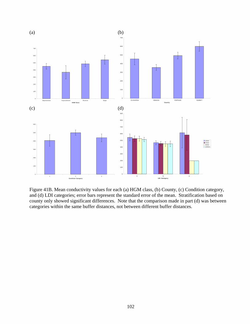
102

(a) (b)

0

100

200

300

400

500

600

700

Depressional Impoundment Riverine Slope

HGM Class

0

100

200

300

400

500

600

700

CUYAHOGA GEAUGA PORTAGE SUMMIT

County (c) (d)

0

100

200

300

400

500

600

1 2 3

Condition Category

0

100

200

300

400

500

600

700

800

900

A N U

LDI Category

100m250m500m1000m

Figure 41B. Mean conductivity values for each (a) HGM class, (b) County, (c) Condition category, and (d) LDI categories; error bars represent the standard error of the mean. Stratification based on county only showed significant differences. Note that the comparison made in part (d) was between categories within the same buffer distances, not between different buffer distances.

103

(a) (b)

0

2

4

6

8

10

12

14

16

Depressional Impoundment Riverine Slope

HGM Class 0

2

4

6

8

10

12

14

CUYAHOGA GEAUGA PORTAGE SUMMIT

County (c) (d)

0

2

4

6

8

10

12

14

16

1 2 3

Condition Category 0

2

4

6

8

10

12

14

A N U

LDI Category

LDI 100LDI 250LDI 500LDI 1000

Figure 41C. Mean percent total carbon values for each (a) HGM class, (b) County, (c) Condition category, and (d) LDI categories; error bars represent the standard error of the mean. Stratification showed significant differences between counties. Note that the comparison made in part (d) was between categories within the same buffer distances, not between different buffer distances.

104

(a) (b)

0

0.0001

0.0002

0.0003

0.0004

0.0005

0.0006

Depressional Impoundment Riverine Slope

HGM Class 0

0.0001

0.0002

0.0003

0.0004

0.0005

0.0006

CUYAHOGA GEAUGA PORTAGE SUMMIT

County (c) (d)

0

0.0002

0.0004

0.0006

0.0008

0.001

0.0012

1 2 3

Condition Category 0

0.0001

0.0002

0.0003

0.0004

0.0005

0.0006

0.0007

A N U

LDI Category

LDI 100LDI 250LDI 500LDI 1000

Figure 41D. Mean total percent nitrogen values for each (a) HGM class, (b) County, (c) Condition category, and (d) LDI categories; error bars represent the standard error of the mean. Stratification based oncounty and LDI categories in the 500 m buffer showed significant differences while other differences did not. Note that the comparison made in part (d) was between categories within the same buffer distances, not between different buffer distances, such that wetlands with agricultural, natural, and urban land-uses in the 500 m buffer had significantly different percent nitrogen values; land-use categories for the 100, 250, and 1000 m buffers showed no such difference.

105

(a) (b)

0

20

40

60

80

100

120

Depressional Impoundment Riverine Slope

HGM Class 0

20

40

60

80

100

120

CUYAHOGA GEAUGA PORTAGE SUMMIT

County (c) (d)

0

20

40

60

80

100

120

140

160

1 2 3

Condition Category 0

20

40

60

80

100

120

A N U

LDI Category

LDI 100LDI 250LDI 500LDI 1000

Figure 41E. Mean total carbon (ug/cc) values for each (a) HGM class, (b) County, (c) Condition category, and (d) LDI categories; error bars represent the standard error of the mean. Stratification based on HGM and county showed significant differences, while other differences did not. Note that the comparison made in part (d) was between categories within the same buffer distances, not between different buffer distances.

106

(a) (b)

0

1

2

3

4

5

6

7

8

Depressional Impoundment Riverine Slope

HGM Class 0

1

2

3

4

5

6

7

8

9

CUYAHOGA GEAUGA PORTAGE SUMMIT

County (c) (d)

0

1

2

3

4

5

6

7

8

9

10

1 2 3

Condition Category 0

1

2

3

4

5

6

7

8

A N U

LDI Category

LDI 100LDI 250LDI 500LDI 1000

Figure 41F. Mean total nitrogen (ug/cc) values for each (a) HGM class, (b) County, (c) Condition category, and (d) LDI categories; error bars represent the standard error of the mean. Stratification based on HGM and county showed significant differences, while other differences did not. Note that the comparison made in part (d) was between categories within the same buffer distances, not between different buffer distances.

107

(a) (b)

0

200

400

600

800

1000

1200

1400

1600

Depressional Impoundment Riverine Slope

HGM Class 0

200

400

600

800

1000

1200

1400

1600

CUYAHOGA GEAUGA PORTAGE SUMMIT

County (c) (d)

0

200

400

600

800

1000

1200

1400

1600

1 2 3

Condition Category 0

500

1000

1500

2000

2500

A N U

LDI Category

LDI 100LDI 250LDI 500LDI 1000

Figure 41G. Mean total phosphorus (ug/cc) values for each (a) HGM class, (b) County, (c) Condition category, and (d) LDI categories; error bars represent the standard error of the mean. Stratification based on county and LDI category 500 m showed significant differences, while other differences did not. Note that the comparison made in part (d) was between categories within the same buffer distances, not between different buffer distances, such that wetlands with agricultural, natural, and urban land-uses in the 500 m buffer had significantly different TP values; land-use categories for the 100, 250, and 1000 m buffers showed no such difference.

108

(a) (b)

0

100

200

300

400

500

600

700

800

Depressional Impoundment Riverine Slope

HGM Class 0

100

200

300

400

500

600

700

CUYAHOGA GEAUGA PORTAGE SUMMIT

County (c) (d)

0

100

200

300

400

500

600

700

1 2 3

Condition Category 0

100

200

300

400

500

600

700

A N U

LDI Category

LDI 100LDI 250LDI 500LDI 1000

Figure 41H. Mean total HCl extracted phosphorus (ug/cc) values for each (a) HGM class, (b) County, (c) Condition category, and (d) LDI categories; error bars represent the standard error of the mean. Stratification based on county and LDI categories in the 250 m buffer showed significant differences while other differences did not. Note that the comparison made in part (d) was between categories within the same buffer distances, not between different buffer distances, such that wetlands with agricultural, natural, and urban land-uses in the 250 m buffer had significantly different HCl extratable phosphorus values; land-use categories for the 100, 500, and 1000 m buffers showed no such difference.

109

(a) (b)

0

0.5

1

1.5

2

2.5

3

3.5

4

Depressional Impoundment Riverine Slope

HGM Class

0

0.5

1

1.5

2

2.5

3

3.5

4

4.5

5

CUYAHOGA GEAUGA PORTAGE SUMMIT

County (c) (d)

0

0.5

1

1.5

2

2.5

3

3.5

4

1 2 3

Condition Category

0

0.5

1

1.5

2

2.5

3

3.5

4

4.5

A N U

LDI Category

LDI 100LDI 250LDI 500LDI 1000

Figure 41I. Mean total water extracted phosphorus (ug/cc) values for each (a) HGM class, (b) County, (c) Condition category, and (d) LDI categories; error bars represent the standard error of the mean. Stratification based on HGM class, county and condition category showed significant differences while others did not. Note that the comparison made in part (d) was between categories within the same buffer distances, not between different buffer distances.

110

(a) (b)

0

20

40

60

80

100

120

140

Depressional Impoundment Riverine Slope

HGM Class 0

20

40

60

80

100

120

CUYAHOGA GEAUGA PORTAGE SUMMIT

County (c) (d)

0

20

40

60

80

100

120

140

1 2 3

Condition Category 0

50

100

150

200

250

A N U

LDI Category

LDI 100LDI 250LDI 500LDI 1000

Figure 41J. Mean total phosphorus-sorption (ug/cc) values for each (a) HGM class, (b) County, (c) Condition category, and (d) LDI categories; error bars represent the standard error of the mean. Stratification based on LDI categories in the 250 and 500 m buffer showed significant differences while other differences did not. Note that the comparison made in part (d) was between categories within the same buffer distances, not between different buffer distances, such that wetlands with agricultural, natural, and urban land-uses in the 250 and 500 m buffer had significantly different phosphorus sorption values; land-use categories for the 100 and 1000 m buffers showed no such difference.

111

(a) (b)

0

1

2

3

4

5

6

7

Depressional Impoundment Riverine Slope

HGM Class

0

1

2

3

4

5

6

7

CUYAHOGA GEAUGA PORTAGE SUMMIT

County (c) (d)

0

2

4

6

8

10

12

14

1 2 3

Condition Category

0

1

2

3

4

5

6

7

8

A N U

LDI Category

LDI 100LDI 250LDI 500LDI 1000

Figure 41K. Mean total nitrate extracted nitrogen (ug/cc) values for each (a) HGM class, (b) County, (c) Condition category, and (d) LDI categories; error bars represent the standard error of the mean. Stratification based on HGM class and county showed significant differences while others did not. Note that the comparison made in part (d) was between categories within the same buffer distances, not between different buffer distances.

112

Figure 42. Box and whisker plots of ORAM scores for different buffer distances (100 m, 250 m, 500 m, 1000 m, 2000 m, 4000 m).

a. 100 meters d. 1000 meters

c. 500 meters f. 4000 meters

b. 250 meters e. 2000 meters

low medium high v ery high

10

20

30

40

50

60

70

80

90

100

OR

AM S

core

low medium high v ery high

10

20

30

40

50

60

70

80

90

100

OR

AM S

core

low medium high v ery high

10

20

30

40

50

60

70

80

90

100

OR

AM S

core

low medium high v ery high

10

20

30

40

50

60

70

80

90

100

OR

AM S

core

low medium high v ery high

10

20

30

40

50

60

70

80

90

100

OR

AM s

core

low medium high very high10

20

30

40

50

60

70

80

90

100

OR

AM s

core

113

0.0

5.0

10.0

15.0

20.0

25.0

30.0

35.0

40.0

45.0

100 m 0.0 2.1 14.6 41.6 30.5 9.4 1.7

250 m 0.0 6.4 19.3 41.2 24.9 6.4 1.7

500 m 1.3 6.9 26.2 36.1 24.5 4.3 0.9

1000 m 2.1 12.0 28.8 36.5 16.3 3.9 0.4

2000 m 1.3 16.3 32.6 32.2 14.6 3.0 0.0

4000 m 3.4 20.6 39.9 24.5 9.9 1.7 0.0

under by 3 under by 2 under by 1 same category over by 1 over by 2 over by 3

Figure 43. The percent agreement between the Level 1 and Level 2 (ORAM) assessments for each buffer distance. Under (by 1, 2, or 3) means the LDI score derived land use class under categorized the wetland lower that what the Level 2 on-site assessment determined, i.e. the wetland was in better condition than predicted by the LDI score; Over (by 1, 2, or 3) means the LDI score over-categorized the wetland, i.e. the wetland was in worse condition than predicted by the LDI score; same category means the LDI and ORAM assessments reached the same result. Note how at the 2000 m and 4000 m buffers, there is an increased tendency to under-categorize wetlands; the opposite is the case at lower buffer distances.

114

Figure 44. Box and whisker plots of average ORAM scores for different Level1:Level2 “agreement” categories for different buffer distances (100 m, 250 m, 500 m, 1000 m, 2000 m, 4000 m). Under (by 1, 2, or 3) means the LDI score derived land use class under categorized the wetland lower that what the Level 2 on-site assessment determined, i.e. the wetland was in better condition than predicted by the LDI score; Over (by 1, 2, or 3) means the LDI score over-categorized the wetland, i.e. the wetland was in worse condition than predicted by the LDI score; same category means the LDI and ORAM assessments reached the same result.

a. 100 meters d. 1000 meters

c. 500 meters f. 4000 meters

b. 250 meters e. 2000 meters

over

by 3

catego

ries

over

by 2

cate

gories

over

by 1

categ

orysame

cat egor

y

under

by 1

catego

ryun

der b

y 2

categ

ories

100

90

80

70

60

50

40

30

20

10

OR

AM S

core

over by 3

catego

ries

over by

2

catego

ries

over b

y 1

categ

or ysam

e

categor

y

unde

r by 1

cate

gory

unde

r by 2

categ

ories

100

90

80

70

60

50

40

30

20

10

OR

AM S

core

over by 3

categor

ies

over by 2

categ

ories

over b

y 1

catego

rysa

me

catego

ry

unde

r by 1

cate

gory

under

by 2

cate

gorie

s

under

by 3

catego

ries

100

90

80

70

60

50

40

30

20

10

OR

AM S

core

over by

3

catego

ries

over b

y 2

categor

ies

over by 1

catego

rysame

categ

ory

under b

y 1

catego

ryun

der b

y 2

categor

ies

unde

r by 3

categor

ies

100

90

80

70

60

50

40

30

20

10

OR

AM S

core

over by 2

categ

ories

over by 1

categorysa

me

cate

gory

under

by 1

catego

ryunde

r by 2

categor

ies

unde

r by 3

cate

gor ies

100

90

80

70

60

50

40

30

20

10

OR

AM S

core

over b

y 2

catego

reis

over b

y 1

catego

rysa

me

catego

ry

under b

y 1

categ

oryund

er by 2

categori

es

under b

y 3

categ

ories

100

90

80

70

60

50

40

30

20

10

OR

AM S

core

115

Figure 45. The percent agreement between the Level 1 and Level 3 (VIBI) assessments for each buffer distance. Under (by 1, 2, or 3) means the LDI score derived land use class under categorized the wetland lower that what the Level 3 on-site assessment determined, i.e. the wetland was in better condition than predicted by the LDI score; Over (by 1, 2, or 3) means the LDI score over-categorized the wetland, i.e. the wetland was in worse condition than predicted by the LDI score; same category means the LDI and VIBI assessments reached the same result.

0

5

10

15

20

25

30

35

40

45

100 m 0 4.7619 14.2857 38.0952 19.0476 19.0476 4.7619

250 m 0 9.5238 33.3333 19.0476 14.2857 19.0476 4.7619

500 m 4.7619 9.5238 42.8571 14.2857 4.7619 23.8095 0

1000 m 9.5238 19.0476 33.3333 23.8095 4.7619 9.5238 0

2000 m 0 33.3333 28.5714 14.2857 4.7619 14.2857 4.7619

4000 m 4.7619 23.8095 42.8571 4.7619 19.0476 4.7619 0

under by 3 under by 2 under by 1 same category over by 1 over by 2 over by 3

116

Figure 46. Box and whisker plots of average VIBI scores different Level1:Level3 “agreement” categories for different buffer distances (100 m, 250 m, 500 m, 1000 m, 2000 m, 4000 m). Under (by 1, 2, or 3) means the LDI score derived land use class under categorized the wetland lower that what the Level 2 on-site assessment determined, i.e. the wetland was in better condition than predicted by the LDI score; Over (by 1, 2, or 3) means the LDI score over-categorized the wetland, i.e. the wetland was in worse condition than predicted by the LDI score; same category means the LDI and ORAM assessments reached the same result.

a. 100 meters d. 1000 meters

c. 500 meters f. 4000 meters

b. 250 meters e. 2000 meters

under-categorized same category over-categorized20

30

40

50

60

70

80

90

100

VIB

I sco

re

under-categorized same category over-categorized

20

30

40

50

60

70

80

90

100

VIB

I sco

re

under-categorized same category over-categorized20

30

40

50

60

70

80

90

100

VIB

I sco

re

under-categorized same category over-categorized20

30

40

50

60

70

80

90

100

VIB

I sco

re

under-categorized same category over-categorized

20

30

40

50

60

70

80

90

100

VIB

I sco

re

under-categorized same category over-categorized20

30

40

50

60

70

80

90

100

VIB

I sco

re

117

Figure 47A. CART model for ORAM scores for all wetlands and their expected thresholds based on CART analysis (overall R2=0.28, cross-validation k=10, R2=0.22). ORAM scores are modified for this analysis by subtracting scores for metric 1 (wetland size) and metric 2 (buffer), making a scoring range of 5 – 70. Red box approximates ORAM score for category 1, gold boxes represent category 2 scores, and green box approximates cut-off for category 3 wetlands.

Mean ORAM 42.4 (±11.7)n=202 Mean

ORAM 37.7 (±13.0)n=37

LDI 100m ?144 Mean ORAM 44.5 (±10.2) n=165

LDI 100m <144

Mean ORAM 27.3 (±13.7) n=10

Mean ORAM 34.8 (±12.5) n=27

Hectare <0.3 Hectare ?0.3 Mean ORAM 42.6 (±9.6) n=122

Mean ORAM 50 (±10.1) n=43

Hectare <4.6 Hectare ?4.6

All Wetlands

Mean ORAM 43.4 (±9.1) n=112 Mean

ORAM 33.9 (±10.8)n=10

LDI 2000m >215

LDI 2000m ?215

Mean ORAM 41.5 (±9.3) n=69

Mean ORAM 46.5 (±7.9) n=43

TP (mg/cc) ? 1.0 TP (mg/cc) < 1.0

118

Mean ORAM 38.0 (±12.2)n=77

Mean ORAM 35.4 (±13.9)n=60

H2O-P (ug/cc) <4.5 Mean ORAM 47.4 (±8.7) n=17

H2O-P (ug/cc) ?4.5

Mean ORAM 29.0 (±12.4) n=15

Mean ORAM 37.5 (±108) n=45

Hectare <0.3 Hectare ?0.3

Mean ORAM 28.9 (±14.8)n=5

Mean ORAM 39.6 (±7.3) n=38

TN (mg/cc) ? 9.2 TN (mg/cc) < 9.2

Depressional Wetlands

Mean ORAM 22.1 (±13.3) n=9

Mean ORAM 41.0 (±6.1) n=5

LDI 500m<135

Figure 47B. CART model for ORAM scores for depressional wetlands and their expected thresholds based on CART analysis (overall R2=0.50, crossvalidation k=10, R2=0.36). ORAM scores are modified for this analysis by subtracting scores for metric 1 (wetland size) and metric 2 (buffer), making a scoring range of 5 – 70. Red box approximates ORAM score for category 1, gold boxes represent category 2 scores, and green box approximates cut-off for category 3 wetlands.

119

Figure 47C. CART model for ORAM scores for riverine wetlands and their expected thresholds based on CART analysis (overall R2=0.52, crossvalidation k=10, R2=0.45). ORAM scores are modified for this analysis by subtracting scores for metric 1 (wetland size) and metric 2 (buffer), making a scoring range of 5 – 70. Gold boxes represent category 2 scores, and green box approximates cut-off for category 3 wetlands.

Mean ORAM44.8 (±11.7)n=71

Mean ORAM 31.2 (±8.1) n=9

LDI 100m ?155

Mean ORAM 46.7 (±9.9) n=62

LDI 100m <155

Mean ORAM 44.2 (±9.3) n=38

Mean ORAM 51.2 (±9.4) n=24

Hectare <4.6 Hectare ?4.6

Riverine Wetlands

Mean ORAM 41.0 (±9.7) n=20

Mean ORAM 48.0 (±6.2) n=18

LDI 4000m <150 LDI 4000m >150

Mean ORAM46.9 (±9.8) n=15

Mean ORAM56.3 (±7.4) n=9

HCl-P(ug/cc)< 480 HCl-P (ug/cc) ?480

Mean ORAM 35.9 (±7.3) n=14

Mean ORAM50.5 (±7.3) n=10

TP (mg/cc) >1 TP (mg/cc) <1

120

Cat1 mod Cat2 Cat2 Cat3 Cuyahoga Urban10

20

30

40

50

60

70

80

90

100

OR

AM v

5

Figure 48A. Comparison of mean ORAM scores in Cuyahoga watershed and Urban wetlands in Franklin County with mean scores from Ohio EPA’s reference wetland dataset. See Table 24 for ANOVA and multiple comparison results.

LQWLH RWLH WLH SWLH bank mit cuy urb

0

50

100

VIBI

sco

re

Figure 48B. Comparison of mean VIBI scores in Cuyahoga watershed, Urban wetlands in Franklin County, mitigation bank sites (bank), individual mitigation sites (mitigation) with mean scores from Ohio EPA’s reference wetland dataset. See Table 24 for ANOVA and multiple comparison results.

121

Figure 49A. Percentage of WETLAND RESOURCE in four categories based on samples of first 50, 100, 125, 150, 200, and 243 points. Refer to Table 24 for actual values.

Figure 49B. Percentage of AVERAGE ORAM SCORES by four categories based on samples of first 50, 100, 125, 150, 200, and 243 points. Refer to Table 24 for actual values.

0%

10%

20%

30%

40%

50%

60%

70%

80%

90%

100%

50 pts 100 pts 125 pts 150 pts 200 pts 243 pts

Category 3

Category 2

modified Category 2

Category 1

0%

20%

40%

60%

80%

100%

50 pts 100 pts 125 pts 150 pts 200 pts 243 pts

Category 3

Category 2

modified Category 2

Category 1

122

Figure 49C. Percentage of ORAM score STANDRD DEVIATION in four categories based on samples of first 50, 100, 125, 150, 200, and 243 points. Refer to Table 24 for actual values.

Figure 49B. Percentage of ORAM score 95% CONFIDENCE INTERVAL by four categories based on samples of first 50, 100, 125, 150, 200, and 243 points. Refer to Table 24 for actual values.

0%

20%

40%

60%

80%

100%

50 pts 100 pts 125 pts 150 pts 200 pts 243 pts

Category 3

Category 2

modified Category 2

Category 1

0%

10%

20%

30%

40%

50%

60%

70%

80%

90%

100%

50 pts 100 pts 125 pts 150 pts 200 pts 243 pts

Category 3

Category 2

modified Category 2

Category 1

123

Appendices

Appendix A - Field Data Sheets

Appendix B - Amphibian Data

Appendix C - Soil Spectral Study

Appendix D - Site List

Appendix E (digital) - Vegetation Data

Appendix F (digital) - Site Data

Appendix G (digital) - Point Maps

BACKGROUND INFORMATION

SITE NAME: SITE ID:

DATE: / / 2 0 0 5 DATA RECORDED BY:

FormReview

HGM Class(codes on back)

Plant Community Class(codes on back)

Primary Secondary Tertiary

. .

. .

Point Number

Modified PointNumber (if applicable)

County

Y N

Y N

Y N

Y N

Y N

Y N

Y N

Y N

180 degree photograph taken.

Site sketch made (aerial or topo.)

ORAM form completed.

Stressor checklist completed.

Wetland determination completed.

Soil samples (6) collected.

Photo log filled out with photograph numbers.

Data sheets QAed after sampling completed.

Y N

Y N

Was there a wetland at the point?If NO, go to next question. If YES, stop.

Was there a wetland within 60 m of the point?If NO, go to next question. If YES, stop.

NONWETLAND CHARACTERIZATION -- Pick One of the Three Options Below.

The soils are NOT hydric andthe area at the point is...

The soils ARE hydric and thearea at the point is...

No determination can be made.Explain below.

Developed with buildings, road, pavement, fill

Farmed

Other (specify)

Developed with buildings, road, pavement, fill

Farmed

Other (specify)

CLASSIFICATION

LOCATION

DATA QUALITY CONTROL

WETLAND PRESENCE

Latitude Longitude

M

Comment required if item answer is no

24290

APPENDIX A

1 of 8

COMMENTS, SITE SKETCHES, ETC.

Class Subclass

I Depression A Permanent inundationB Regular inundationC Seasonal inundationD Seasonal saturation

II Impoundment A BeaverB Human

III Riverine A HeadwaterB MainstemC Channel

IV Slope A HeadwaterB MainstemC IsolatedD Fringing

V Fringing A ReservoirB Natural lake

VI Coastal Not applicaple

VII Bog A Strongly ombrotrophicB Moderately ombrotrophicC Weakly ombrotrophic

Class Subclass

1 Forest A Swamp forestB Bog forestC Forest seep

2 Emergent A MarshB Wet meadowC Open bog

3 Shrub A Shrub swampB Tall shrub bogC Tall shrub fen

HYDROGEOMORPHIC CLASSIFICATION PLANT COMMUNITY CLASSIFICATION

SITE ID: DATE: / / 2 0 0 5

BACKGROUND INFORMATION FormReview

24290

APPENDIX A

2 of 8

WETLAND DETERMINATION FORM

WETLAND VEGETATION

Y N U Is the canopy dominated by wetland tree species?

Y N U Is the subcanopy (shrubs, small trees) dominated by wetland shrub or tree species?

Y N U Is the herb layer dominated by wetland species?

Is the overall vegetation of the area dominated by hydrophytic vegetation?(If no (N) or unable to determine (U), explain in comments.)Y N U

Inundated

Saturated in upper 30 cm (12 in)

Water marks

Drift lines

Sediment deposits

Drainage patterns in wetland

Oxidized root channels in upper 30 cm (12 in)

Water stained leaves

Other

HYDROLOGY INDICATORSPrimary Secondary

SOIL CHARACTERISTICS

Y N

Y N

HYDRIC SOIL INDICATORS

Histosol (peat or muck upper 80 cm)

Histic epipedon (peat or muck upper 40 cm)

Sulfur odor

Aquic moisture regime

Gleyed or low chroma soils

Concretions

High organic content in sandy soils

Organic streaking in sandy soils

Listed local hydric soil list

Listed national hydric soil list

WETLAND DETERMINATION

Y N Hydrophytic vegetation present

Y N Wetland hydrology present

Y N Hydric soils present

Y N Is this sampling point within a wetland

SITE NAME: DATE: / / 2 0 0 5INVESTIGATORS:

COUNTY:

POINT NO.:

MODIFIEDLATITUDE:

Matrix Color Mottle Color % Mottle Hydr. Cond.TextureOxid. Roots TEXTURE:LM = Loam SAL = Sandy loam SIL = Silty loamCL = Clay loam SACL = Sandy clay loamSICL = Silty clay loam C = Clay SAC = Sandy claySIC = Silty clay P = Peat M = MuckHYDR. COND.:I = Inundated S = Saturated M = Moist D = Dry

5 cm

20 cm

COMMENTS

.

.MODIFIEDLONGITUDE:

53294

APPENDIX A

3 of 8

Common Wetland Trees Silver maple Red maple Green ash Black ash Swamp white oak Pin oak American elm Slippery elm

Other Trees SometimesEncountered in Wetlands Black gum White pine American beech Tulip tree Birches (Betula) Cottonwood Swamp cottonwood Pumpkin ash

Common Wetland Shrub and Subcanopy TreeSpecies Spicebush (Lindera) Winterberry (Ilex) Chokecherry (Aronia) Buttonbush (Cephalanthus) Musclewood (blue beech) (Carpinus) Willows (Salix spp.) Arrowwood (Viburnum) Highbush blueberry (Vaccinium) Poison sumac (Toxicodendron) Alder (Alnus) Swamp rose (Rosa) Dogwood (Cornus) Spiraea Buckthorn (Rhamnus)

Common Wetland Graminoid Species Sedges (Carex) Bulrush (Scirpus, Schoenoplectus, Bolboschoenus) Spikerush (Eleocharis) Umbrella sedge (Cyperus) Three-way sedge (Dulichium) Twigrush (Cladium) True rush (Juncus) Bur-reed (Sparganium) Manna grasses (Glyceria) Wood reed (Cinna) Bluejoint grasses (Calamagrostis) Prairie cord grass (Spartina) Reed canary grass (Phalaris) Giant reed (Phragmites) Cutgrass (Leersia) Cattails (Typha)

Common Emergent Wetland Forbs Angelica Aster spp. Bedstraw (Galium) Beggar ticks (Bidens) Boneset (Eupatorium) Ditch stonecrop (Penthorum) False nettle (Boehmeria) Godenrods (Solidago, Euthamia) Hedge nettles (Stachys) Horehounds (Lycopus) Iris spp. Jewelweed (Impatiens) Joe-pye weeds (Eupatorium) Marsh marigold (Caltha) Marsh St. John's Wort (Triadenum, Hypericum) Marsh violets (Viola) Mountain mints (Pycnanthemum) Lobelias (cardinal flower, great lobelia) Loosestrife, native (Lysamachia) Loosestrife, purple (Lythrum salicaria) Loosestrife, swamp (Decodon) Loosestrife, winged (Lythrum alatum) Skullcaps (Scutellaria) Skunk cabbage (Symplocarpus) Smartweeds (Polygonum) Spring cress (Cardamine) Swamp buttercups (Ranunculus) Swamp dock (Rumex) Swamp mallow (Hibiscus) Swamp milkweed (Asclepias) Swamp saxifrage (Saxifraga) Swamp thistle (Cirsium) Sweet flag (Acorus) Water hemlock (Cicuta)

Common Aquatic Wetland Forbs Arrowheads (Sagittaria) Bladderworts (Utricularia) Buttercups, aquatic (Ranunculus flabellaris, R. longirostris) Coontails (Ceratophyllum) Duckweeds, common (Lemna minor) Duckweeds, uncommon (Lemna trisulca) Duckweed, large (Spirodela) Mermaid weed (Proserpinaca) Milfoils (Myriophyllum) Naiads (Najas) Pickerel weed (Pontederia) Pondweeds (Potamogeton) Spatterdocks (Nuphar) Water lilies (Nymphaea) Water meal (Wolffia) Water plaintain (Alisma) Watershield (Brasenia)

Common Wetland Ferns Cinnamon fern (Osmunda cinnamomea) Horsetail ferns (Equisetum) Royal fern (Osmunda regalis) Sensitive fern (Onoclea) Spinulose shield fern (Dryopteris carthusiana)

APPENDIX A

4 of 8

SITE NAME: SITE ID:

DATE: / / DATA RECORDED BY:

OHIO RAPID ASSESSMENT METHODFormReview

2 0 0 5

Page 1 of 2

Metric 1

Metric 1. Wetland Area (size) Metric 2. Upland buffer and surrounding land use2a. Calculate average buffer width. Select only one and assign score.

2b. Intensity of surrounding land use. Select one or take average of two. Metric 2

Metric 3. Hydrology3a. Sources of water. Score all that apply.

3b. Connectivity. Score all that apply.

3c. Maximum water depth. Select only oneand assign score.

3d. Duration inundation/saturation. Score one ortake average of two.

3e. Modifications to natural hydrologic regime.Score one or take average of two.3b

3c

3a

3e

3d

Metric 3

4a. Substrate disturbance.Score one or take average of two.

4b. Habitat development.Select only one and assign score.

4c. Habitat alteration. Score one ortake average of two. Metric 4

Metric 4. Habitat Alteration and Development

4a

4b

4c

Check all disturbances observedDitchTile

DikeWeir Point source (non-stormwater)

Filling/gradingRoadbed/RR track

DredgingOther

Stormwater input

Check all disturbances observedMowingGrazingClearcutting

Woody debris removalSedimentation

Toxic pollutantsShrub/sapling removal

Selective cuttingHerbaceous/aquatic bed removalFarming

DredgingNutrient enrichment

SUBTOTAL - Page 1

SCORE

(max 20 pts)

(max 30 pts)

(max 14 pts)

(max 6 pts)

7 WIDE-Buffers average 50 m (164 ft) or more around wetland perimeter 4 MEDIUM-Buffers average 25 to <50 m (82 to <164 ft) around wetland perimeter 1 NARROW-Buffers average 10 to <25 m (32 to <82 ft) around wetland perimeter 0 VERY NARROW-Buffers average <10 m (<32 ft) around wetland perimeter

7 VERY LOW - 2nd growth or older forest, prairie, savannah, wildlife area, etc. 5 LOW - Old fields (>10 years), shrubland, young second growth forest 3 MODERATELY HIGH - Residential, fenced pasture, park, conservation tillage, new fallow field 1 HIGH - Urban, industrial, open pasture, row cropping, mining, construction

5 High pH groundwater 3 Other groundwater 1 Precipitation 3 Seasonal/intermittent surface water 5 Perennial surface water (lake or stream)

1 100 year flood plain 1 Between stream/lake and other human use 1 Part of wetland/upland (e.g. forest) complex 1 Part of riparian or upland corridor

3 >0.7 m (>27.6 in) 2 0.4 to 0.7 m (15.7 to 27.6 in) 1 <0.4 m (<15.7 in)

4 Semi to permanently inundated/saturated 3 Regularly inundated/saturated 2 Seasonally inundated 1 Seasonally saturated in upper 30 cm (12 in)

12 None or none apparent 7 Recovered 3 Recovering 1 Recent or no recoverey

4 None or none apparent 3 Recovered 2 Recovering 1 Recent or no recoverey

7 Excellent 6 Very good 5 Good 4 Moderately good 3 Fair 2 Poor to fair 1 Poor

9 None or none apparent 6 Recovered 3 Recovering 1 Recent or no recoverey

6 >50 acres (>20.2 ha)

5 25 to <50 acres (10.1 to 20.2 ha)

4 10 to <25 acres (4 to <10.1 ha)

3 3 to <10 acres (1.2 to <4 ha)

2 0.3 to <3 acres (0.12 to <1.2 ha)

1 0.1 to <0.33 acres (0.04 to <0.12 ha)

0 <0.1 acres (0.04 ha)

28238

APPENDIX A

5 of 8

Page 1 of 2

SITE ID: DATE: / / 2 0 0 5

Page 2 of 2

OHIO RAPID ASSESSMENT METHODFormReview

Metric 5. Plant Communities, interspersion, microtopography

5a. Wetland Vegetation Communities.Circle the score of all present using 0 to 3cover scale using tables 1-3 as a guide.

Table 1. Vegetation Community Cover Scale(see table 2 for description of quality)

5a

(max 20 pts)

Metric 5

5b. Horizontal (plan view) interspersion.Select only one.

Table 2. Narrative Description of Vegetation Quality

5b

5c. Coverage of invasive plants. Add ordeduct points for coverage.

5d. Microtopography. Circle the score of all presentusing 0 to 3 cover scale using table 4 as a guide.

Table 4. Microtopography Cover Scale

5c

5d

Mark all that apply and score as indicated. Metric 6

Metric 6. Special Wetlands

Grand Total (max 100 pts)

Condition Score (Page 1 + Metric 5) (Max 90 points)

(max 10 pts)

10 Bog

10 Old growth forest10 Fen

5 Mature forested wetland

10 Lake Erie coastal/tributary wetland - unrestricted hydrology 5 Lake Erie coastal/tributary wetland - restricted hydrology

10 Lake plain sand prairies (Oak Openings)10 Relict wet prairies

10 Significant migratory songbird/water fowl habitat or useage10 Known occurence state/federal threatened or endangered species

-10 Category 1 wetland. See question 1 qualitative rating

Present but <0.1 ha (0.247 a) contiguous area.

Present and either comprises small part of wetland's vegetation and is ofmoderate quality, or comprises a significant part, but is of low quality.

Present and either comprises significant part of wetland's vegetation and isof moderate quality, or comprises a small part and is of high quality.

Present and either comprises significant part, or more, of wetland'svegetation and is of high quality.

1

2

3

Table 3. Mudflat and Open Water Class Quality

Low spp diversity and/or predominance of nonnative or disturbance tolerantnative species.

Native spp are dominant component of the vegetation, although nonnativeand/or disturbance tolerant native spp can also be present, and speciesdiversity moderate to moderately high, but generally w/o presence of rarethreatened or endangered spp.

A predominance of native species, with nonnative spp and/or disturbancetolerant native spp absent or virtually absent, and high spp diversity andoften, but not always, the presence of rare, threatened or endangered spp.

Low

Mod

High

Present but <0.1ha (0.247 acres) contiguous area

Low 0.1 to <1ha (0.247 to 2.47 acres)

Moderate 1 to <4ha (2.47 to 9.88 acres)

High 4ha (9.88 acres) or more

0

1

2

3

Page 1Subtotal

SCORE

0 1 2 30 1 2 30 1 2 30 1 2 30 1 2 30 1 2 30 1 2 3

Aquatic bedEmergentShrubForestMudflatsOpen waterOther (list below)

5 High 4 Moderately high 3 Moderate 2 Moderately low 1 Low 0 None

-5 Extensive >75% cover -3 Moderate 25-75% cover -1 Sparse 5-25% cover 0 Nearly absent <5% cover 1 Absent

Vegetated hummucks/tussucks 0 1 2 3Coarse woody debris >15 cm (6 in) 0 1 2 3Standing dead >25 cm (10 in) dbh 0 1 2 3Amphibian breeding pools 0 1 2 3

0

Present small amounts or, if more common, of marginalquality.

Functionally absent (present in very small amounts.)

Present in moderate amounts, but not of highest quality orin small amounts of highest quality.

Present in moderate or greater amounts and of highest quality.

0

1

2

3

28238

APPENDIX A

6 of 8

HYDROLOGIC MODIFICATION

TILE DRAINL M H

DITCHL M H

DikeL M H

Weir/damL M H

STORMWATER INPUTS/CULVERTSL M H

POINT SOURCE (NON-STORMWATER)L M H

L M H

Roadbed/railroadL M H

OtherL M H

L M H

SEDIMENTATION

L M H

Sediment deposits/plumesL M H

Siltiness on ground or vegetationL M H

URBAN/ROAD STORMWATER INPUT/CULVERTL M H

HIGH BOD

L M H

OtherL M H

Severe vegetation stressL M H

TOXIC CONTAMINANTS

OBVIOUS SPILLS, DISCHARGES, PLUMES, ODORSL M H

Wildlife impacts (e.g. tumors, abnormalities, etc.)L M H

OtherL M H

Adjacent industrial sites, proximity of railroadL M H

PENN STATE STRESSOR CHECKLIST

Active/recently active adjacent construction, plowing,heavy grazing or forest harvesting

Filling, grading, dredging (of wetland/waterbodyor immediate buffers)

Dominant presence (>50% of vegetation) of sedimenttolerant plants (see list)

Excessive denisity of aquatic plants or algal matsin water column.

Excessive deposition or dumping of organic waste(e.g. leaves, grass, clippings, woody debris, etc.).

L M H

VEGETATION ALTERATION

MowingL M H

GrazingL M H

Tree cutting (>50% canopy removal)L M H

Brush cutting (mechanized removal of shrubs/saplings)L M H

Removal of woody debrisL M H

OtherL M H

Aquatic weed control (mechanical or herbicide)L M H

Excessive herbivory (deer, muskrat, geese, carp, etc.)L M H

Evidence of chemical defoliationL M H

Dominant presence (>50% of the vegetation) of exoticor aggressive plant species (see list)

SITE NAME: SITE ID:

DATE: / / 2 0 0 5 DATA RECORDED BY:

Direct discharges of organic wastewater or material (e.g.milkhouse waste, food-processing waste, otherwastewater sources).

CHECK BOX IN CATEGORY HEADING IF ANY OF THE STRESSOR TYPES LISTED FOR THE CATEGORY ARE CHECKED.

Mark all observed. Mark all observed.

Mark all observed.

Mark all observed.

Mark all observed.

Form Review

Page 1 of 2

Dead/dying treesL M H

L M H

L M H

Eroding banks/slopesL M H

OtherL M H

45684

APPENDIX A

7 of 8

EUTROPHICATION AND NUTRIENT ENRICHMENT

L M H

Other (e.g. signs of excess nutrients - methane odor, dead fish, etc.)L M H

DIRECT DISCHARGES FROM AG. FEEDLOT, MANURE PITS, ETC.L M H

DIRECT DISCHARGES FROM SEPTIC OR SEWAGE TREATMENT SYSTEMSL M H

Heavy or moderate formation of algal matsL M H

ACIDIFICATION

ACID MINE DRAINAGE DISCHARGESL M H

OtherL M H

ADJACENT MINED LANDS/SPOIL PILESL M H

Excessively clear waterL M H

Absence of expected biotaL M H

OtherL M H

L M H

L M H

THERMAL ALTERATION

OtherL M H

Significant increase in water temperatureL M H

Moderate increase in water temperatureL M H

Other (e.g. evident use of road salt)L M H

Obvious increase in concentration of dissolved saltsL M H

Dominant presence (>50% of vegetation) of nutrient tolerant species(e.g. uniform stand of exotic/aggressive species)

Buffer Type

Natural Forest

Shrub/Sapling

Perennial Herb

Other (list)

Buffer Width (m) Buffer Score(from table)

Buffer Width (m)Buffer Type*

Natural Forest

Perennial Herb

Shrub/Sapling

Other*If exactly one-half of two buffer types, take half the sum.

>100 30-100 10-30 3-10 0-3

14 12 10 8 6

12 10 8 6 4

10 8 6 4 2

00000

PENN STATE STRESSOR CHECKLIST

SITE ID: DATE: / / 2 0 0 5

CHECK BOX IN CATEGORY HEADING IF ANY OF THE STRESSOR TYPES LISTED FOR THE CATEGORY ARE CHECKED.

Mark all observed.

Mark all observed.

Mark all observed.

Mark all observed.

Mark all observed.

High concentration of suspendedsolids in water column.

Moderate concentration ofsuspended solids in water column.

Page 2 of 2

Form Review

SALINITY

TURBIDITY

45684

APPENDIX A

8 of 8

APPENDIX BAMPHIBIAN DATA

SiteCode Site Applicable type AmphIB

I

AQAI

AQAI Metr

ic

RA Tol

RA Tol Metr

ic

RA Sen

RA Sen

Metr

ic

Sal.Sp.

Sal. M

etric

WF/S

S

WF/S

S Metr

ic

comments

SITE2001 Alexander Rd not sampleable * * * * * * * * * * *

SITE2005 Old Forge Rd no, bog 0 2.25 0 1 0 0 0 0 0 no 0 2 passes (1&2)

SITE2008 Bartholomew Rd no, marsh 0 0 0 0 0 0 0 0 0 no 0 no amphibians collected

SITE2013 Ward Rd no, marsh 3 3 3 1 0 0 0 0 0 no 0

SITE2014 Brecksville yes 30 4.13 3 0.723 3 0.1702 7 3 7 yes 10

SITE2015 Black Rd yes 10 3 3 0.5 7 0 0 1 0 no 0 2 passes (1&2)

SITE2016 Wake Robin not sampleable * * * * * * * * * * *

SITE2017 Quail Hollow yes 30 6.86 10 0.029 10 0.97066 10 0 0 no 0

SITE2020 Thut no, riverine forest 6 3.15 3 0.976 0 0.02439 3 1 0 no 0

SITE2023 Bath Rd yes 0 2.86 0 1 0 0 0 0 0 no 0 2 passes (1&2)

SITE2025 Rhinehart no, riverine marsh 3 3 3 1 0 0 0 0 0 no 0 2 passes (1&2)

SITE2027 Hasbrouck yes 40 6.87 10 0.034 10 0.96585 10 1 0 yes 10

SITE2028 Bridge Creek not sampleable * * * * * * * * * * *

SITE2029 Twinsburg no, riverine 3 3 3 1 0 0 0 0 0 no 0 2 passes (1&2)

SITE2031 Miller no, marsh 0 0 0 0 0 0 0 0 0 no 0 1 pass (1)

SITE2032 Aquilla Rd no, riverine marsh 0 2.15 0 1 0 0 0 0 0 no 0

SITE2033 Goodyear yes 40 6.9 10 0.025 10 0.975 10 0 0 yes 10 2 passes (1&2)

SITE2034 Oak Knolls no, riverine forest 0 2.2 0 1 0 0 0 0 0 no 0 2 passes (2&3)

SITE2036 Tare Creek no, riverine marsh 0 2.87 0 1 0 0 0 0 0 no 0

SITE2037 Wingfoot Lake no, marsh 3 3 3 1 0 0 0 0 0 no 0

SITE2040 South Rider Rd no, riverine marsh * * * * * * * * * * *

SITE2042 Marsh Wetlands no, riverine marsh * * * * * * * * * * *

last revised 8/19/2007 B1 Amhibs_Hoga_Report.xls

APPENDIX BAMPHIBIAN DATA

Jeffe

rson s

al.

spott

ed sa

l.

sm. m

outh

sal.

red sp

ot. ne

wt

sprin

g pee

per

w. cho

rus fro

g

bullfr

og

green

frog

leopa

rd fro

g

wood f

rog

Site # Site Name AMBJEF AMBMAC AMBTEX NOTVIR PSECRU PSETRI RANCAT RANCLA RANPIP RANSYL2001 Alexander Rd * * * * * * * * * *

2005 Old Forge Rd * * * * 0.75 * 0.25 * * *

2008 Bartholomew Rd * * * * * * * * * *

2013 Ward * * * * * 1.00 * * * *

2014 Brecksville 0.11 0.09 * 0.09 * * 0.07 0.64 0.02 *

2015 Black Rd * * 0.50 * 0.50 * * * * *

2016 Wake Robin * * * * * * * * * *

2017 Quail Hollow * * * * 0.02 0.01 0.00 0.00 * 0.97

2020 Thut * * * 0.02 * * * 0.98 * *

2023 Bath Rd * * * * 0.14 * * 0.86 * *

2025 Rhinehart * * * * * * * 1.00 * *

2027 Hasbrouck * 0.01 * * * 0.01 * 0.02 0.00 0.95

2028 Bridge Creek * * * * * * * * * *

2029 Tinkers Oxbow * * * * * * * 1.00 * *

2031 Miller * * * * * * * * * *

2032 Aquilla Rd * * * * 0.06 * 0.01 0.12 0.82 *

2033 Goodyear Bog * * * * * * * 0.25 * 0.98

2034 Oak Knolls * * * * * * 0.80 0.20 * *

2036 Tare Creek * * * * * * * 0.87 0.13 *

2037 Wingfoot Lake * * * * * * * 1.00 * *

2040 South Rider Rd * * * * * * * * * *

2042 Marsh Wetlands * * * * * * 0.51 0.49 * *

last revised 8/19/2007 B2 Amhibs_Hoga_Report.xls

OHIO ENVIRONMENTAL PROTECTION AGENCY

BIOGEOCHEMICAL CHARACTERIZATION AND SPECTRAL CALIBRATION OF WETLAND SOIL SAMPLES FROM THE CUYAHOGA RIVER BASIN

FEBRUARY 14, 2006

DR. MATT COHEN WETLAND BIOGEOCHEMISTRY LABORATORY

SOIL AND WATER SCIENCE DEPARTMENT UNIVERSITY OF FLORIDA

APPENDIX C

1 of 38

Summary

This report summarizes the findings of an examination of wetland soils from throughout

the Cuyahoga River basin in northern Ohio. The soil study was implemented in two phases; the

first phase was analysis of a subset of the 1685 soil samples collected for a full range of

biogeochemical indicators; the second phase was development and use of predictive models

between these observed indicators and high resolution diffuse reflectance spectra. The latter

method is an emerging technique for rapid, low-cost characterization of environmental samples.

In this work, the spectral technique (visible/near infrared reflectance spectroscopy – VNIRS)

allowed comprehensive characterization (21 soil properties) of a large number of wetland soils

(>1400 samples). This report summarizes the laboratory analyses, calibration efficiency between

VNIR spectra and site-level variability in soil properties. Our general conclusion is that VNIRS

represents a useful tool for characterization of chemical and physical properties of environmental

samples; for some analytes, prediction efficiency is excellent (organic matter, total nitrogen, total

carbon, total phosphorus, total calcium), while for others it is inadequate (KCl-extractable

nitrates, water-extractable phosphorus, total conductivity). For the remaining analytes (pH, HCl-

extractable P, bulk density, P-sorption capacity, total metals [K, Mg, Zn, Cu, Fe, Al, Pb, Na])

prediction efficiencies were adequate for applications in which high-sample throughput is

required (e.g., resource or condition mapping), but less than adequate for high-accuracy

applications (e.g., regulatory testing).

APPENDIX C

2 of 38

Introduction and Background

Analytical spectroscopy is a proven technology for the rapid non-destructive assessment of

materials, including plastics, industrial reagents, minerals and agricultural products. Spectral

reflectance signature libraries of numerous material samples and composites have been cataloged

(e.g. Clark 1999); from these libraries, unknown samples are interpreted for functional and

qualitative properties. There are many platforms and analytical schemes for obtaining and

interpreting spectral properties of samples. The application used in this work, which measures

diffuse visible/near infrared reflectance (VNIR), involves collecting high-resolution optical

signatures (e.g. 1-nm bandwidths) from a sample illuminated by a high intensity full spectrum

light source in the visible (350-750 nm) and near-to-mid infrared (750-2500 nm) regions of the

electromagnetic spectrum.

Fig. 1 – Typical spectral responses of green vegetation, dry vegetation (litter) and soil. Optical absorbance and reflectance features are composite responses of the organic and inorganic constituents of each material (USGS 1999).

Under controlled conditions, reflectance signatures arise due to electronic excitation of

atoms and vibrational stretching and bending of structural groups of atoms that form molecules

and crystals. For example, fundamental vibrational features for organic matter functional groups

are observed in the mid- to thermal-infrared (2.5-25 µm) portion of the spectrum; however,

overtones of these fundamental features occur at fractions of the fundamental frequency, which

fall within the range typical of DRS (700-1000 nm and 1000-2500 nm). Clay minerals and

APPENDIX C

3 of 38

common cations also exhibit distinctive spectral reflectance characteristics due to light

interference, facilitating rudimentary mineralogical description.

Despite the widespread application of analytical/descriptive spectroscopy to the

characterization of relatively pure molecular mixtures, quantitative inference of soil quality

indicators from spectral reflectance is limited by the heterogeneous character of the soil system.

In particular, soil represents a complex mixture of spectrally active constituents, and efforts to

unmix spectral responses for characterization efforts on bulk samples have been relatively

unsuccessful. Quantitative spectroscopy treats the characterization question differently; rather

than trying to use diagnostic features of a spectrum for inferring presence of particular organic

functional groups or minerals, multivariate analytical tools are used to infer composition and

concentration indirectly (i.e., statistically) from complex, strongly co-linear reflectance spectra.

The emergence and proliferation in the last decade of powerful statistical data mining tools (e.g.

Partial Least Squares [PLS] regression, Classification and Regression Trees [CART] and

Multivariate Adaptive Regression Splines [MARS]) has allowed researchers to develop efficient

predictive correlations between spectral response characteristics and a wide array of standard soil

and plant functional parameters (Ben- Dor and Banin 1995, Kooistra et al. 1997, Foley et al.

1998, Gillon et al. 1999, Chen et al. 2002). The method continues to be tested in a wide array of

ecological regions; recent work (Cohen et al. 2005) demonstrated applicability to a wide array of

potential ecosystem indicators in wetland systems with low ash-content soils.

Formal methods for analyzing soil archives for which laboratory evaluations have been

performed have been developed (Shepherd and Walsh 2002). This approach is founded on the

development of Spectral Reflectance Libraries (SRLs). SRLs consist of archived soils for which

spectral response curves and controlled laboratory analyses of functional indicators have been

collected. From the SRLs, calibrations are developed to correlate reflectance to functional

measurements; validated models can then be used to infer soil properties in incoming sample

soils for the suite of laboratory indicators without direct analysis. The indicator analytes that

have exhibited association with spectra in other studies include cation concentrations (Ca, Mg,

Fe, Al, Na), soil organic matter and ash content, soil texture and soil phosphorus. Preliminary

evidence suggests that reliable models can be developed to infer organic carbon quality (e.g.

lignin content - citation), organic mineralization rates (Bouchard et al. 2003, Fystro 2002), soil

hydraulic properties (Cohen et al. submitted), and various measures of toxic contamination

APPENDIX C

4 of 38

(Kooistra et al. 1997). While for many of these parameters, it is strong co-linearity with readily

observable soil attributes (e.g. soil carbon, soil clay content) and not direct reflectance effects

that are being observed, our research (Cohen et al. 2005) has shown that spectral observations

provide a measure of the soil system that offer non-redundant information about its composition.

The approach proposed for this study will facilitate rapid quantitative inference of a suite

of soil physical and chemical properties directly from reflectance characteristics. Our experience

suggests that, given effective data and sample management protocols, 100-200 samples can be

processed by a single technician in one day, and spectral quality assurance and prediction can be

automated so that results emerge for all parameters simultaneously in real-time. Given

extremely basic sample pre-processing, this offers tremendous throughput potential. Further, the

cost of analysis are significantly reduced compared with conventional laboratory costs, which

allows strategic spatial and temporal sampling, high-resolution surveys of soil condition and

statistically powerful inference of the effects of human activities on soil function to be developed

with relative ease.

Study Objectives and Protocols

As part of a large assessment study of wetlands throughout the Cuyahoga River basin,

soils were collected from 287 wetlands sites. At each site, 6 samples were collected (total N =

1685); from 231 sites, one sample selected for full laboratory characterization (see Table 1 for

list of selected analytes). All samples were analyzed spectrally (details given below). Our

objectives were:

1) Develop statistical predictive relationships between the measured soil properties and soil

spectra, and use standard prediction evaluation methods to determine which analytes can

be successfully predicted using a samples spectral signature.

2) Apply the predictive relationship to the 1454 samples for which only spectral data were

obtained.

3) Determine within- and between-site variability in spectrally predicted soil properties.

Below, we present the methods used for soil characterization and obtaining spectral

signatures. Our results are reported in three stages: 1) soil biogeochemistry, 2) soil spectra and

predictive modeling, and 3) model extension and site level summary.

APPENDIX C

5 of 38

Methods

Soil Biogeochemical Measurements

The list of soil analytes under examination in this work includes bulk soil properties (pH,

conductivity, organic matter content, bulk density), nutrient pools (total P, total N, total C, HCl-

extractable P, water extractable P, KCl-extractable nitrates), P sorption capacity, and total metals

(K, Na, Ca, Mg, Al, Fe, Cd, Pb, Cu, Zn).

Soil pH and conductivity were determined by a Fisher Scientific multi-meter on 10 g wet

soil after equilibrating with 20 mL of distilled deionized water. Organic matter content (%) was

determined from residue after ashing at 550 oC (Anderson, 1976). Total P was determined by

combusting approximately 0.2-0.5 g oven-dried, finely ground soil at 550o C for 4 hrs, digesting

the ash with 6M HCl and continuous heating on a hot plate, and filtering through No. 41

Whatman filter (Anderson 1976), followed by analysis of P by automated ascorbic acid method

(Method 365.1: USEPA 1993). Total C and N were determined on dried, ground soil samples by

dry combustion (Nelson and Sommers 1996) using a Carlo-Erba NA-1500 CNS Analyzer (Haak-

Buchler Instruments, Saddlebrook, NJ). HCl-extractable P was determined by extraction of 0.5

g dry soil in 25 mL 1 N HCl with shaking for 3 hrs, filtration through 0.45µm membrane filter,

and analysis of P by automated ascorbic acid method (Method 365.1: USEPA 1993). Water

extractable P was determined by extraction of the wet soil equivalent of 2.5 g soil dry weight in

25 mL of distilled deionized water with shaking for 1 hr, followed by filtration through 0.45 µm

membrane filter (Kuo 1996) and analysis of P by automated ascorbic acid method (Method

365.1: USEPA 1993). KCl-extractable NO3- was determined by extraction of 2 g of dry soil in

25 mL of 2.0 M KCl with shaking for 1 hour, centrifuging and filtration through a Whatman #41

filter followed by colorimetric nitrate determination (Mulvaney 1996). P sorption was done

using single point isotherms with 1.0 g of dry soil in 10 mL of 0.01 M KCl solution with 100

ppm phosphate followed by 24 hours of shaking, filtration through 0.45 µm filters and analysis

of P by automated ascorbic acid method (Method 365.1: USEPA 1993). Total metals

concentrations were determined using the solution from the Total P protocol, followed by

analysis using ICP (EPA method 200.7). All analyses were performed by the Wetland

Biogeochemistry Laboratory except ICP measures of total metals, which was performed at UF’s

Analytical Research Laboratory (ARL).

APPENDIX C

6 of 38

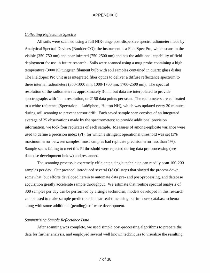
Collecting Reflectance Spectra

All soils were scanned using a full NIR-range post-dispersive spectroradiometer made by

Analytical Spectral Devices (Boulder CO); the instrument is a FieldSpec Pro, which scans in the

visible (350-750 nm) and near infrared (750-2500 nm) and has the additional capability of field

deployment for use in future research. Soils were scanned using a mug probe containing a high

temperature (3000 K) tungsten filament bulb with soil samples contained in quartz glass dishes.

The FieldSpec Pro unit uses integrated fiber optics to deliver a diffuse reflectance spectrum to

three internal radiometers (350-1000 nm; 1000-1700 nm; 1700-2500 nm). The spectral

resolution of the radiometers is approximately 3-nm, but data are interpolated to provide

spectrographs with 1-nm resolution, or 2150 data points per scan. The radiometers are calibrated

to a white reference (Spectralon – LabSphere, Hutton NH), which was updated every 30 minutes

during soil scanning to prevent sensor drift. Each saved sample scan consists of an integrated

average of 25 observations made by the spectrometers; to provide additional precision

information, we took four replicates of each sample. Measures of among-replicate variance were

used to define a precision index (PI), for which a stringent operational threshold was set (3%

maximum error between samples; most samples had replicate precision error less than 1%).

Sample scans failing to meet this PI threshold were rejected during data pre-processing (see

database development below) and rescanned.

The scanning process is extremely efficient; a single technician can readily scan 100-200

samples per day. Our protocol introduced several QAQC steps that slowed the process down

somewhat, but efforts developed herein to automate data pre- and post-processing, and database

acquisition greatly accelerate sample throughput. We estimate that routine spectral analysis of

300 samples per day can be performed by a single technician; models developed in this research

can be used to make sample predictions in near real-time using our in-house database schema

along with some additional (pending) software development.

Summarizing Sample Reflectance Data

After scanning was complete, we used simple post-processing algorithms to prepare the

data for further analysis, and employed several well known techniques to visualize the resulting

APPENDIX C

7 of 38

data. First, dataset end-members were identified based on organic matter content (% loss-on-

ignition), and plotted to offer an example of the spectral variability.

Data post-processing is an optional step in the data analysis process, but one shown to

have significant influence on model prediction efficiency. For this effort, data post-processing

consisted of spectral resampling (reduce by a factor of 10 the dimensionality of the spectra to

permit more manageable analysis) and derivative transformation (to eliminate between sample

effects due to ambient light conditions, optical set-up and specular reflectance). Other post-

processing techniques (scatter correction, normalization) were not done because previous efforts

indicated that these conferred no advantage in spectral predictive modeling.

To visualize the spectral data prior to analysis, we used a principal components analysis

on the derivative transformed, resampled data. This step is particularly useful to ascertain if the

calibration data subsample (231 laboratory analyzed samples) is spectrally representative of the

population. The PCA also permits the identification of spectral outliers that may exert

significant leverage on the calibration procedure.

Developing Spectral Prediction Models

After acquiring and pre-processing the spectral data, and consolidating/normalizing the

soil biogeochemical data, multivariate spectral modeling was started. Two methods were

initially compared because the research literature contains examples where both have been

shown to be superior with respect to prediction accuracy and model stability. The first and most

commonly applied is called partial least squares regression; this technique is also known as

projection-to-latent structures regression or PLS. The basic concept of this approach is to extract

canonical variables from the predictor data (spectra in this case) that are observed to be

correlated with the target variable (soil chemical properties). The decomposition of the

predictor-by-sample matrix into principal components is done conditioned to maximize the

covariance between the PCs and the target parameters.

PLS is a classical linear statistical tool and, as such, sensitive to certain anomalies in

predictor and target variables. Among these are the assumption of normality and presence of

outliers; for this reason, post-processing tools and visualization are critical.

Another method gaining favor in the research literature (Brown et al. 2005) for its

flexibility and accuracy is a non-parametric data mining tool called stochastic gradient boosted

APPENDIX C

8 of 38

tree regression (GBT). Tree-based analytical methods are based on recursive binary splitting of

the target data; it is analogous to well-known decision trees. At each binary split (or parent

node), the algorithm identifies the variable and level that maximizes the purity or minimizes the

within-node deviance of the resulting two nodes (daughter nodes). This algorithm, applied

recursively, allows partitioning of the original data into increasingly pure subsets based on

simply decision rules. In a regression setting, each sample allocated to a particular terminal node

is given the mean value of that node, and this value is compared to the observed value.

There are several primary problems with tree-based regression including optimality

problems and over-fitting. In gradient boosted tree (GBT) models, large sets of smaller trees

(nnodes ~ 3; selecting the single best split from among all predictors) are grown, each building on

the last by incorporating the previous residuals in an additive weighted expansion; observations

with larger residuals are preferentially weighted in subsequent iterations. This generic algorithm

is rapid to implement, allows inclusion of predictors for which pairwise associations are

relatively weak, and can be used to develop fits with non-normal data and for non-linear

responses (Friedman 2002).

For soft-modeling of spectra, or chemometric modeling, one critical requirement is a data

set large enough to permit separation of the sample data into a training data set and a verification

data set. Many of the statistical tools have a propensity to over-fit to the training data, so to

provide a reasonable measure of predictive accuracy under implantation conditions, a hold-out

validation data set is retained. In our work, model development was performed using only the

231 training samples; we explored the accuracy and stability of the calibrations under various

calibration and validation set conditions (50-80% for calibration). Assessing model utility is

always made based on the efficiency of predicting hold-out validation observations.

Model Diagnostics

Because the process of chemometric modeling is inferential and not mechanistic, a set of

robust diagnostics are required to ensure that observed relationships are not spurious, and to

compare between model types. Further, model diagnostics provide the necessary information to

determine if the prediction efficiency meets the minimum requirements of the desired

application. We use a set of well established diagnostics to evaluate the fit between predicted

and observed values for each of the soil properties evaluated.

APPENDIX C

9 of 38

There are three primary model diagnostics for continuous prediction. The first is the

familiar coefficient of determination (r2), which describes the goodness-of-fit between predicted

an observed as a fraction of the total variance in the latter. While this index is familiar to most

analysts, there are no well-defined utility thresholds for discriminating between useful and less

useful models. Model significance (that is, the probability that the observed relationship is nill

given the data) is of no utility for this effort. We report the r2 value because of its general appeal.

A second index is mean error (standard error of calibration or validation), which

measures the average deviation between predicted and observed values. Because the regression

error terms are typically normal, the mean squared error is strongly influenced by samples with

large residuals. However, the SEC/SEV value is of considerable utility for evaluating the

accuracy of the model, particularly where the level of accuracy necessary for a given application

can be specified. The SEC/SEV is not a useful index for comparing across models to determine

relative accuracy; for that measure we use an index developed in the chemical engineering

literature for chemometrics. The RPD value scales the SEV value by the population standard

deviation (i.e. RPD = SD/SEV). Large values indicate high relative efficiency. The research

literature consistently interprets values greater than 2.0 as having immediate predictive utility,

values less than 1.5 are of limited utility for even first-estimate applications, while parameters

with model RPD values between 1.5 and 2 are of variable utility depending on the application.

Finally, we use the slope and intercept of the fitted line to determine model bias. The

expected slope is 1.0 and models that deviate significantly from that value systematically over-

estimate large observed values and underestimate small observed values. Slopes less than 1

reverse this problem, with low and high observations predicted closer to the population mean.

The intercept value is indicative of systematic over- or under-estimation over the entire data

range. Intercept errors are unusual, but slope errors are common, mainly for model algorithms

that average multiple predictions (e.g. GBT).

Model Application and Site Level Summary

Once validated models have been selected, they can be immediately applied to the

remaining samples for which spectral information is available. There are two levels of error to

contend with for these data – first, there is error associated with the spectral prediction, which

can be evaluated based on the information obtained during the calibration. The second type of

APPENDIX C

10 of 38

error, which emerges when the multiple (n ~ 6) samples at each site are evaluated is associated

with internal spatial variability resulting from hydrologic and nutrient enrichment gradients.

After application of the spectral model to the full soil dataset, we examined the error (variability)

associated with each site. Sites were rank ordered by site mean concentration for each of the 20

analytes, and plotted with error bars representing the standard deviation around the site mean.

This gives both an estimate of the within-site variability (especially when the within-site

variability is compared with the population standard deviation) and between-site variability. The

direct interpretation of the linkages between the site mean (and variability) and indicators of

ecological condition represent an important next step in the use of these data.

Results I: Soil Biogeochemical Characterization

Table 1 summarizes the observed concentrations of the soil biogeochemical indicators;

note that cadmium was measured, but the data were eliminated from further analysis because

nearly all the samples were below the analytical detection limit. Some of the analytes required

normalization to meet the assumptions of the analytical methods – these are listed in Table 1.

Table 1. Summary of soil observations from wetlands in the Cuyahoga River basin.

Soil Parameter N Mean Minimum Maximum Std.Dev. Transform pH 231 5.71 3.74 7.61 0.82 none Cond. (µmhos) 231 487.48 1.07 2050.00 340.51 Ln Bulk Dens. (g/cm3) 230 1.31 0.18 2.77 0.60 none Moisture Content (%) 230 0.45 0.08 0.90 0.18 none LOI (%) 231 0.24 0.03 0.87 0.18 Ln TP (mg/kg) 231 1076.01 260.07 3712.32 569.26 Ln TN (g/kg) 231 6.82 0.63 29.41 5.94 Ln TC (g/kg) 231 102.93 6.81 475.65 94.87 Ln HCl-P (mg/kg) 231 413.37 27.69 2530.90 393.83 Ln H2O-P (mg/kg) 231 3.38 0.23 70.58 6.58 Ln NO3-N (mg/kg) 231 3.60 0.16 67.60 9.30 Ln P-Sorption (mg/g) 231 78.47 36.16 134.33 18.38 none Potassium (mg/kg) 231 23.63 1.75 52.90 11.09 none Calcium (mg/kg) 231 28.48 2.41 129.50 24.96 Ln Magnesium (mg/kg) 231 14.63 1.23 47.60 5.90 Ln Zinc (mg/kg) 231 0.55 0.14 2.37 0.26 Ln Copper (mg/kg) 231 0.06 0.00 0.66 0.06 Ln Iron (mg/kg) 231 127.79 0.00 2080.40 145.66 Ln Aluminum (mg/kg) 231 121.73 17.96 264.70 46.03 none Cadmium (mg/kg) 231 0.00 0.00 0.03 0.00 Ln Lead (mg/kg) 231 0.18 0.03 1.21 0.12 Ln Sodium (mg/kg) 231 2.49 1.01 26.54 1.95 Ln

APPENDIX C

11 of 38

Figure 2 shows the inter-correlations between the observed soil properties. Among the

criticisms of the spectral method is that it measures only organic matter content; because OM

content is correlated with many other aspects of soil performance, spectral predictive

relationships are spurious. While there is some merit to this critique, the degree to which this is

indeed the case can be assessed by examining the correlation structures in Figure 2. Further,

Table 2 summarizes the correlations with OM for all 20 analytes.

Fig. 2 – Matrix plots of a) bulk soil parameters measured and b) soil total metal concentrations. Shown are correlation structures and histograms for normality transformed data (see Table 1).

APPENDIX C

12 of 38

Table 2. Summary of correlation structure for soil biogeochemical observations.

pH

Bul

k D

ens.

P-So

rptio

n (m

g/g)

TrC

ond

TrLO

I

TrTP

TrTN

TrTC

TrH

Cl-P

TrH

2O-P

TrN

O3-

N

K

Al

TrC

a

TrM

g

TrZn

TrC

u

TrFe

TrPb

Bulk Dens. 0.05 - P-Sorption (mg/g) -0.29 -0.53 - TrCond 0.30 -0.30 0.08 - TrLOI -0.19 -0.78 0.56 0.22 - TrTP -0.10 -0.61 0.56 0.13 0.68 - TrTN -0.28 -0.79 0.61 0.19 0.95 0.74 - TrTC -0.25 -0.79 0.58 0.21 0.95 0.69 0.98 - TrHCl-P 0.17 -0.42 0.35 0.22 0.36 0.78 0.41 0.38 - TrH2O-P -0.14 -0.47 0.16 0.07 0.61 0.60 0.62 0.61 0.44 - TrNO3-N 0.00 -0.09 0.06 0.15 0.24 0.30 0.25 0.23 0.19 0.24 - K 0.22 0.06 0.08 0.11 -0.18 0.15 -0.16 -0.21 0.25 -0.15 0.17 - Al 0.03 -0.02 0.18 -0.03 -0.04 0.31 -0.01 -0.06 0.24 -0.04 0.12 0.75 - TrCa 0.40 -0.56 0.27 0.43 0.65 0.48 0.60 0.63 0.46 0.39 0.27 -0.01 -0.06 - TrMg 0.49 0.06 0.01 0.24 -0.16 0.13 -0.17 -0.17 0.31 -0.18 0.20 0.80 0.59 0.30 - TrZn 0.29 -0.28 0.21 0.19 0.21 0.48 0.21 0.20 0.57 0.18 0.21 0.44 0.40 0.43 0.60 - TrCu 0.23 -0.41 0.24 0.27 0.42 0.49 0.40 0.42 0.51 0.30 0.32 0.25 0.26 0.59 0.39 0.51 - TrFe 0.31 0.00 0.11 0.10 -0.08 0.19 -0.09 -0.11 0.27 -0.36 0.07 0.39 0.38 0.15 0.49 0.46 0.20 - TrPb -0.10 -0.40 0.33 0.12 0.47 0.50 0.50 0.53 0.29 0.37 0.17 0.04 0.17 0.31 0.12 0.49 0.42 0.06 - TrNa 0.27 -0.13 0.21 0.21 0.10 0.16 0.08 0.08 0.26 -0.02 0.13 0.46 0.31 0.31 0.49 0.32 0.29 0.26 0.12

We observe that there are indeed strong associations with organic matter content

(particularly for some of the metals, Cu and Pb, that may be harder to determine spectrally).

Only comparison of these Pearson correlation coefficients (r-values) with the observed model

efficiencies (summarized using r2-values) will illustrate the degree to which this confounding

factor is problematic.

Results II: Soil Spectral Characterization and Predictive Modeling

Spectral Summary

A summary of the full spectral data set is not possible graphically; to demonstrate the

degree of difference, we have selected nine representative samples from the entire gradient of

organic matter contents observed in the training data set. The spectra (derivative transformed)

are shown in Fig. 3 in an effort to demonstrate the relatively subtle differences that permit

prediction of soil chemical properties.

APPENDIX C

13 of 38

We can summarize the full data set by data compression techniques. Principal

components analysis permits the full data set (n = 1685) to be displayed using a reduced number

of latent variables that describe most of the data set variance. Principal components 1 through 4

captured nearly 90% of the original data set variance, and are plotted in scatterplots in Fig. 4.

Notably, while most of the dataset variance can be explained with this small number of

independent variables, the rotation techniques used for spectral calibration (PLS in particular)

often observe important predictive information from many more predictive axes (PCs). This

suggests that, while data compression is useful for visualizing bulk variability, more subtle

methods are critical for direct interpretation of the spectral response.

The maximal utility of the PCA method for dataset visualization is to determine the

degree to which the 231 training samples adequately represent the full dataset. In Fig. 4, the

PCA was done on all data simultaneously, but the points representing the 231 training samples

are delineated from the other samples. The results suggest that, in general the training data set is

representative of the population except for along PC4 (Fig. 4b).

Fig. 3 – Selected spectrographs for Cuyahoga wetlands spectral database. Spectrographs were selected along a gradient of organic matter content (LOI), and are reported as 1st derivative relative reflectance. Spectral diagnostic features are the location and depth of soil reflectance and absorbance bands. For organic matter content, the depth of absorbance in bands 1360 and 2210 are particularly diagnostic. Similarly, for phosphorus prediction, the spectral response at band 1920 is important.

APPENDIX C

14 of 38

Fig. 4 – Principal components analysis for all spectral samples; crosses represent the 1454 samples with spectra only and the grey circles represent the 231 calibration samples. Four PC axes are presented which in total explain nearly 90% of the total dataset spectral variance. Note, however, that the partial least squares (PLS) algorithm used for spectral predictive modeling often employs more than four latent components for prediction.

APPENDIX C

15 of 38

Chemometric Model Results

After comparison of the two methods (PLS and GBT) for spectral prediction, we

concluded that the additional time required to develop GBT models was not warranted; in most

cases PLS provided improved validation accuracy, reduced model complexity and much greater

model portability. As such, the results of the GBT effort are omitted from this report.

The PLS results are summarized in Figures 5 and 6. The individual fits (for calibration

and validation) are shown in Figures 7-26. For all models, we selected the cross-validation

scheme where 80% of the data were used for calibration and models were evaluated using the

remaining 20% (selected randomly). The reason for this are summarized in Figure 27; we

observe across almost all parameters that the use of a smaller fraction of the 231 training samples

resulted in weaker models. This may suggest that there is some lower bound to the number of

samples necessary to develop a reliable and generic spectral reflectance library. We note that for

calibrations developed using much larger data sets (n > 2000) we generally observe that

validation accuracy starts to level off at between 300 and 500 samples in the training set. Using

190 samples for training appears to be adequate, but future and broader iterations of this effort

should consider the need for a larger SRL from which to determine the necessary spectral

relationships.

APPENDIX C

16 of 38

Fig. 5 – Validation relative performance determinant (RPD) for standard soil properties. Thresholds of 1.5 and 2.0 are marked. Properties are in raw units unless preceded by Tr, which indicates natural log transform prior to calibration.

Fig. 6 – Validation relative performance determinant (RPD) for total metals concentrations. Thresholds of 1.5 and 2.0 are marked. Properties are in raw units(mg/kg) unless preceded by Tr, which indicates natural log transform prior to calibration.

APPENDIX C

17 of 38

Fig. 7 – Predicted vs. observed pH for calibration (80%) and validation (20%).

Fig. 8 – Predicted vs. observed bulk density for calibration (80%) and validation (20%).

APPENDIX C

18 of 38

Fig. 9 – Predicted vs. observed P sorption for calibration (80%) and validation (20%).

Fig. 10 – Predicted vs. observed total conductivity for calibration (80%) and validation (20%). Values are natural log transformed prior to calibration.

APPENDIX C

19 of 38

Fig. 11 – Predicted vs. observed organic matter (loss-on-ignition; LOI) for calibration (80%) and validation (20%). Values are natural log transformed prior to calibration.

Fig. 12 – Predicted vs. observed total phosphorus for calibration (80%) and validation (20%). Values are natural log transformed prior to calibration.

APPENDIX C

20 of 38

Fig. 13 – Predicted vs. observed total nitrogen for calibration (80%) and validation (20%). Values are natural log transformed prior to calibration.

Fig. 14 – Predicted vs. observed total carbon for calibration (80%) and validation (20%). Values are natural log transformed prior to calibration.

APPENDIX C

21 of 38

Fig. 15 – Predicted vs. observed HCl-extractable phosphorus for calibration (80%) and validation (20%). Values are natural log transformed prior to calibration.

Fig. 16 – Predicted vs. observed water extractable phosphorus for calibration (80%) and validation (20%). Values are natural log transformed prior to calibration.

APPENDIX C

22 of 38

Fig. 17 – Predicted vs. observed KCl-extractable nitrate for calibration (80%) and validation (20%). Values are natural log transformed prior to calibration.

Fig. 18 – Predicted vs. observed total potassium for calibration (80%) and validation (20%).

APPENDIX C

23 of 38

Fig. 19 – Predicted vs. observed for total aluminum for calibration (80%) and validation (20%).

Fig. 20 – Predicted vs. observed total calcium for calibration (80%) and validation (20%). Values are natural log transformed prior to calibration.

APPENDIX C

24 of 38

Fig. 21 – Predicted vs. observed total magnesium for calibration (80%) and validation (20%). Values are natural log transformed prior to calibration.

Fig. 22 – Predicted vs. observed total zinc for calibration (80%) and validation (20%). Values are natural log transformed prior to calibration.

APPENDIX C

25 of 38

Fig. 23 – Predicted vs. observed total copper for calibration (80%) and validation (20%). Values are natural log transformed prior to calibration.

Fig. 24 – Predicted vs. observed total iron for calibration (80%) and validation (20%). Values are natural log transformed prior to calibration.

APPENDIX C

26 of 38

Fig. 25 – Predicted vs. observed total lead for calibration (80%) and validation (20%). Values are natural log transformed prior to calibration.

Fig. 26 – Predicted vs. observed total sodium for calibration (80%) and validation (20%). Values are natural log transformed prior to calibration.

APPENDIX C

27 of 38

Results III: Spectral Prediction of Soil Properties and Site-Level Synthesis

Fig. 27 – Summary of site level mean and distribution for spectrally predicted pH.

Fig. 28 – Summary of site level mean and distribution for spectrally predicted bulk density.

APPENDIX C

28 of 38

Fig. 27 – Summary of site level mean and distribution for spectrally predicted P sorption.

Fig. 28 – Summary of site level mean and distribution for spectrally predicted conductivity (ln transf).

APPENDIX C

29 of 38

Fig. 29 – Summary of site level mean and distribution for spectrally predicted loss-on-ignition (ln transf.)

Fig. 30 – Summary of site level mean and distribution for spectrally predicted total P (ln transf.).

APPENDIX C

30 of 38

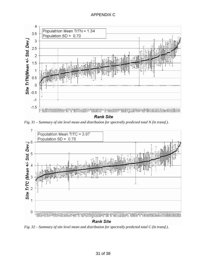
Fig. 31 – Summary of site level mean and distribution for spectrally predicted total N (ln transf.).

Fig. 32 – Summary of site level mean and distribution for spectrally predicted total C (ln transf.).

APPENDIX C

31 of 38

Fig. 33 – Summary of site level mean and distribution for spectrally predicted HCl-P (ln transf.).

Fig. 34 – Summary of site level mean and distribution for spectrally predicted HCl-P (ln transf.).

APPENDIX C

32 of 38

Fig. 35 – Summary of site level mean and distribution for spectrally predicted NO3-N (ln transf.).

Fig. 36 – Summary of site level mean and distribution for spectrally predicted Total K.

APPENDIX C

33 of 38

Fig. 37 – Summary of site level mean and distribution for spectrally predicted Total Al.

Fig. 38 – Summary of site level mean and distribution for spectrally predicted total Ca (ln transf.).

APPENDIX C

34 of 38

Fig. 39 – Summary of site level mean and distribution for spectrally predicted total Mg (ln transf.)

Fig. 40 – Summary of site level mean and distribution for spectrally predicted total Zn (ln transf.).

APPENDIX C

35 of 38

Fig. 41 – Summary of site level mean and distribution for spectrally predicted total Cu (ln transf.).

Fig. 42 – Summary of site level mean and distribution for spectrally predicted total Fe (ln transf.).

APPENDIX C

36 of 38

Fig. 43 – Summary of site level mean and distribution for spectrally predicted total Pb (ln transf.).

Fig. 44 – Summary of site level mean and distribution for spectrally predicted total Na (ln transf.). Discussion and Conclusions

APPENDIX C

37 of 38

Future Work

This work has measured biogeochemical properties at 231 wetland sites throughout the

Cuyahoga River basin, and developed predictive models that relate a much less expensive soil

property (spectral response) to these expensive measures of soil condition; these models were

extrapolated to an additional 1454 samples for which only spectral response information was

available. This report presents the absolute and relative efficiencies of spectral prediction for

each of the 20 analytes, and suggests that for many of them spectral prediction may be a useful

rapid assessment tool. Given this observation, we project three important tasks to be

accomplished in future work:

1) Understand the spatial and temporal variability of the spectral predictions for purposes of

efficient sampling and interpretation.

2) Examination of relationships between soil biogeochemical indicators and measures of

biological condition based on community composition and landscape matrix.

3) Development of direct spectral correlates with assessed biological/ecological condition.

This work can be accomplished as the data for biogeochemical condition and ecological

condition are fused.

APPENDIX C

38 of 38

APPENDIX DSITE LIST

SITE_ID Site Same as1 Same as2 Group type Modified** Fate*** If not Wetland Area name LONG_DDN83 LAT_DDN83WCW02352-2001 2001 OEPA 1 N 5 Congress Lake Region -81.256167 41.024223WCW02352-2002 2002 OEPA 0 na 0 on slope, no wetland w/in 60m Breakneck Cr Region -81.328714 41.162531WCW02352-2003 2003 OEPA 3 3 Hudson Swamp - Brandwine Cr Swamp -81.499664 41.276865WCW02352-2004 2004 OEPA 1 N 3 Middle Upper Cuyahoga River -81.079486 41.545586WCW02352-2005 2005 OEPA 1 N 5 Breakneck Cr Region -81.320538 41.079073WCW02352-2006 2006 OEPA 0 0 Area filled or never wetland Cuyahoga County -81.770699 41.436833WCW02352-2007 2007 2119 2335 OEPA 3 3 Hudson Swamp - Brandwine Cr Swamp -81.481719 41.235575WCW02352-2008 2008 OEPA 1 N 5 Middle Upper Cuyahoga River -81.227580 41.367039WCW02352-2009 2009 OEPA 3 3 Breakneck Cr Region -81.253966 41.129797WCW02352-2010 2010 OEPA 0 0 prior converted farmland Lower Upper Cuyahoga (Portage Co.) -81.248942 41.317215WCW02352-2011 2011 OEPA 0 N 0 Streetsboro school built on site Streetsboro - L Rockwell Region -81.326165 41.236681WCW02352-2012 2012 OEPA 3 3 Middle Upper Cuyahoga River -81.232495 41.354750WCW02352-2013 2013 OEPA 1 N 5 Greater Akron -Mogadore Res Region -81.399283 41.029004WCW02352-2014 2014 OEPA 1 N 5 Cuyahoga Valley Region -81.591098 41.325138WCW02352-2015 2015 OEPA 1 N 5 Cuyahoga Valley Region -81.602523 41.249462WCW02352-2016 2016 OEPA 1 Y 5 Middle Upper Cuyahoga River -81.284601 41.422496WCW02352-2017 2017 OEPA 1 Y 5 Stark Co site Congress Lake Region -81.312969 40.973292WCW02352-2018 2018 OEPA 3 3 Breakneck Cr Region -81.320611 41.119225WCW02352-2019 2019 OEPA 0 na 0 reservoir deep water Streetsboro - L Rockwell Region -81.308356 41.209325WCW02352-2020 2020 OEPA 1 N 5 Middle Upper Cuyahoga River -81.272509 41.334236WCW02352-2021 2021 OEPA 0 0 Cuyahoga Valley Region -81.586547 41.204961WCW02352-2022 2022 OEPA 0 N 0 Point located in WWT lagoon Cuyahoga County -81.663454 41.438815WCW02352-2023 2023 OEPA 1 Y 5 Cuyahoga Valley Region -81.573615 41.171461WCW02352-2024 2024 OEPA 3 3 Middle Upper Cuyahoga River -81.237796 41.428703WCW02352-2025 2025 OEPA 1 N 5 Breakneck Cr Region -81.271396 41.071575WCW02352-2026 2026 OEPA 0 N 0 Not a wetland Lower Upper Cuyahoga (Portage Co.) -81.188279 41.306222WCW02352-2027 2027 OEPA 1 Y 5 Hudson Swamp - Brandwine Cr Swamp -81.405358 41.227069WCW02352-2028 2028 OEPA 1 N 5 2028, 2108, 2356 all separate assessment u Middle Upper Cuyahoga River -81.184677 41.417910WCW02352-2029 2029 OEPA 1 Y 5 Upper Tinkers Creek -81.430100 41.305162WCW02352-2030 2030 OEPA 3 3 Middle Upper Cuyahoga River -81.124362 41.434071WCW02352-2031 2031 OEPA 1 Y 5 Greater Akron -Mogadore Res Region -81.405671 41.118388WCW02352-2032 2032 2360 OEPA 1 N 5 includes 2360 Upper Cuyahoga River -81.175500 41.525006WCW02352-2033 2033 OEPA 1 N 5 Greater Akron -Mogadore Res Region -81.357623 41.003634WCW02352-2034 2034 OEPA 1 Y 5 Streetsboro - L Rockwell Region -81.336436 41.174959WCW02352-2035 2035 OEPA 3 3 Streetsboro - L Rockwell Region -81.375481 41.217519WCW02352-2036 2036 2348 OEPA 1 Y 5 includes 2348 Upper Cuyahoga River -81.114302 41.472940WCW02352-2037 2037 OEPA 1 Y 5 Greater Akron -Mogadore Res Region -81.363799 41.019140WCW02352-2038 2038 OEPA 0 0 No wetland w/in 60m of point Cuyahoga County -81.682389 41.338641WCW02352-2039 2039 OEPA 0 0 No wetland w/in 60m of point Hudson Swamp - Brandwine Cr Swamp -81.507418 41.157946WCW02352-2040 2040 OEPA 1 Y 5 Upper Cuyahoga River -81.177514 41.469216WCW02352-2041 2041 OEPA 3 3 Breakneck Cr Region -81.246726 41.095693WCW02352-2042 2042 OEPA 1 N 5 Lower Upper Cuyahoga (Portage Co.) -81.219181 41.278899WCW02352-2043 2043 6 6

last revised 8/19/2007 D1 FixedtrackingSpreadsheet_FinalFinal.xls

APPENDIX DSITE LIST

SITE_ID Site Same as1 Same as2 Group type Modified** Fate*** If not Wetland Area name LONG_DDN83 LAT_DDN83WCW02352-2044 2044 OEPA 1 N 5 Upper Cuyahoga River -81.249860 41.390145WCW02352-2045 2045 2173 OEPA 1 N 5 2173 is part of this Upper Tinkers Creek -81.379889 41.291183WCW02352-2046 2046 OEPA 3 3 Middle Upper Cuyahoga River -81.091257 41.433660WCW02352-2047 2047 OEPA 0 0 Not a wetland Greater Akron -Mogadore Res Region -81.505987 41.090288WCW02352-2048 2048 OEPA 1 N 5 Upper Cuyahoga River -81.158522 41.561185WCW02352-2049 2049 OEPA 1 N 5 Breakneck Cr Region -81.255583 41.076206WCW02352-2050 2050 G3 1 N 1 Breakneck Cr Region -81.275536 41.152416WCW02352-2051 2051 K1-ECS 1 N 1 Lower Upper Cuyahoga (Portage Co.) -81.289030 41.257712WCW02352-2052 2052 SF 0 4 photo Cuyahoga County -81.435363 41.350455WCW02352-2053 2053 P+L 1 N 1 Cuyahoga Valley Region -81.700705 41.165488WCW02352-2054 2054 K1 +P&J 1 N 1 Hudson Swamp - Brandwine Cr Swamp -81.508512 41.311518WCW02352-2055 2055 S4 0 na 0 park Cuyahoga Valley Region -81.525104 41.217126WCW02352-2056 2056 G3 1 N 1 Upper Cuyahoga River -81.161051 41.451921WCW02352-2057 2057 S4 1 N 1 Congress Lake Region -81.306229 41.027131WCW02352-2058 2058 K1-ECS 1 N 1 Lower Upper Cuyahoga (Portage Co.) -81.268061 41.181854WCW02352-2059 2059 2387 G3+J 1 Y 1 2387 is part of this Greater Akron -Mogadore Res Region -81.451442 41.149842WCW02352-2060 2060 JMMM 1 N 1 Middle Upper Cuyahoga River -81.155693 41.379179WCW02352-2061 2061 2389 K1-LE 1 N 1 2389 not near 2061 Upper Tinkers Creek -81.434982 41.313643WCW02352-2062 2062 JMMM 1 N 1 Middle Upper Cuyahoga River -81.157761 41.417770WCW02352-2063 2063 K2-John 1 N 1 Breakneck Cr Region -81.354409 41.129467WCW02352-2064 2064 3 3 Upper Cuyahoga River -81.061791 41.564237WCW02352-2065 2065 S4 3 3 Congress Lake Region -81.264890 41.007416WCW02352-2066 2066 K1-L&E 1 N 1 Streetsboro - L Rockwell Region -81.370649 41.180422WCW02352-2067 2067 K2 1 N 1 Upper Tinkers Creek -81.392363 41.272757WCW02352-2068 2068 2396 John 1 N 1 Upper Cuyahoga River -81.077686 41.488135WCW02352-2069 2069 3 3 Breakneck Cr Region -81.297125 41.091143WCW02352-2070 2070 K2 0 na 0 deep forest Cuyahoga Valley Region -81.582712 41.296851WCW02352-2071 2071 S4 1 N 1 Hudson Swamp - Brandwine Cr Swamp -81.484282 41.174592WCW02352-2072 2072 G3 1 N 1 Middle Upper Cuyahoga River -81.212950 41.455334WCW02352-2073 2073 G3 1 N 1 Breakneck Cr Region -81.264893 41.106165WCW02352-2074 2074 2138 2242 K1-ECS 1 N 1 points probably different assessment units, v Lower Upper Cuyahoga (Portage Co.) -81.218384 41.262410WCW02352-2075 2075 K1-LECS 1 N 1 Upper Tinkers Creek -81.378143 41.280096WCW02352-2076 2076 K3+L 1 N 1 Middle Upper Cuyahoga River -81.245475 41.403908WCW02352-2077 2077 3 3 Upper Tinkers Creek -81.394654 41.297774WCW02352-2078 2078 G3 1 N 1 Cuyahoga County -81.485812 41.443910WCW02352-2079 2079 S4 3 3 Hudson Swamp - Brandwine Cr Swamp -81.501157 41.280426WCW02352-2080 2080 P+L 1 Y 1 Upper Cuyahoga River -81.142670 41.565163WCW02352-2081 2081 G3 0 N 0 CODED WRONG = 0 DEVELOPED ON HYDBreakneck Cr Region -81.235383 41.096588WCW02352-2082 2082 G3 1 N 1 Breakneck Cr Region -81.303600 41.143077WCW02352-2083 2083 K1-ECS 1 N 1 Streetsboro - L Rockwell Region -81.319245 41.267903WCW02352-2084 2084 K3 1 N 1 Cuyahoga County -81.428200 41.363667WCW02352-2085 2085 2361 K2 1 N 1 Cuyahoga Valley Region -81.679363 41.134178WCW02352-2086 2086 SF 0 4 photo Cuyahoga County -81.502001 41.351932

last revised 8/19/2007 D2 FixedtrackingSpreadsheet_FinalFinal.xls

APPENDIX DSITE LIST

SITE_ID Site Same as1 Same as2 Group type Modified** Fate*** If not Wetland Area name LONG_DDN83 LAT_DDN83WCW02352-2087 2087 K2 1 N 1 Cuyahoga Valley Region -81.565758 41.291064WCW02352-2088 2088 G3 0 N 0 Middle Upper Cuyahoga River -81.169723 41.444172WCW02352-2089 2089 K2-CC 1 N 1 Greater Akron -Mogadore Res Region -81.312007 41.069657WCW02352-2090 2090 2258 2386 K1-ECS 1 N 1 Lower Upper Cuyahoga (Portage Co.) -81.254807 41.181534WCW02352-2091 2091 K1-L&E 1 N 1 Upper Tinkers Creek -81.371103 41.199310WCW02352-2092 2092 2260 K1-L&CS 1 N 1 Lower Upper Cuyahoga (Portage Co.) -81.181029 41.349130WCW02352-2093 2093 K3+L 1 N 1 Upper Tinkers Creek -81.396923 41.320982WCW02352-2094 2094 JMMM 0 na 0 pond Middle Upper Cuyahoga River -81.166377 41.406559WCW02352-2095 2095 2263 G3 1 N 1 points probably different assessment units, v Streetsboro - L Rockwell Region -81.366313 41.121788WCW02352-2096 2096 K1+E 0 na 0 Upper Cuyahoga River -81.143297 41.583162WCW02352-2097 2097 S4 1 N 1 Congress Lake Region -81.317593 40.991791WCW02352-2098 2098 K1 0 na 0 forest/hydric soil Streetsboro - L Rockwell Region -81.311828 41.180911WCW02352-2099 2099 K2-L 1 N 1 Upper Tinkers Creek -81.375382 41.235354WCW02352-2100 2100 John 1 Y 1 2100 not same point as 2036 and 2348 Upper Cuyahoga River -81.106327 41.469932WCW02352-2101 2101 K2 1 Y 1 Cuyahoga Valley Region -81.628059 41.166347WCW02352-2102 2102 K2 0 N 0 river bank Cuyahoga Valley Region -81.604675 41.362154WCW02352-2103 2103 S4 3 na 3 Cuyahoga County -81.549464 41.164063WCW02352-2104 2104 G3 1 Y 1 Middle Upper Cuyahoga River -81.243950 41.444460WCW02352-2105 2105 K2-L 3 3 John has folder 2005 Greater Akron -Mogadore Res Region -81.327805 41.074364WCW02352-2106 2106 K1-LE 1 N 1 Lower Upper Cuyahoga (Portage Co.) -81.185885 41.322789WCW02352-2107 2107 K1-L&E 1 N 1 Streetsboro - L Rockwell Region -81.385536 41.179589WCW02352-2108 2108 John 1 N 1 2028, 2108, 2356 all separate assessment u Middle Upper Cuyahoga River -81.189637 41.421814WCW02352-2109 2109 2373 K1+P&J 1 N 1 Upper Tinkers Creek -81.392697 41.288553WCW02352-2110 2110 G3 1 N 1 Upper Cuyahoga River -81.151613 41.442390WCW02352-2111 2111 K1-L&E 1 N 1 Streetsboro - L Rockwell Region -81.410328 41.138300WCW02352-2112 2112 P+L 1 N 1 Upper Cuyahoga River -81.172130 41.544179WCW02352-2113 2113 G3 0 na 0 forest upland, developed Breakneck Cr Region -81.275734 41.125319WCW02352-2114 2114 K1+E 1 N 1 Lower Upper Cuyahoga (Portage Co.) -81.251778 41.324031WCW02352-2115 2115 K1+P 1 N 1 Streetsboro - L Rockwell Region -81.336539 41.232994WCW02352-2116 2116 G3 1 Y 1 Cuyahoga County -81.479993 41.422476WCW02352-2117 2117 2341 K3 1 N 1 inclues 2341 Greater Akron -Mogadore Res Region -81.403097 41.015477WCW02352-2118 2118 K2 0 N 0 upland area near creek Cuyahoga County -81.575394 41.355325WCW02352-2119 2119 2007 2335 Marie 3 3 John denied Hudson Swamp - Brandwine Cr Swamp -81.483669 41.240610WCW02352-2120 2120 John 1 N 1 Middle Upper Cuyahoga River -81.287623 41.419016WCW02352-2121 2121 K2 1 Y 1 Streetsboro - L Rockwell Region -81.367450 41.098409WCW02352-2122 2122 SF 0 4 photo Cuyahoga County -81.767086 41.423655WCW02352-2123 2123 Marie 3 3 according to John Hudson Swamp - Brandwine Cr Swamp -81.474122 41.238336WCW02352-2124 2124 2208 JMMM 1 N 1 2208 is part of this Middle Upper Cuyahoga River -81.152342 41.385137WCW02352-2125 2125 3 3 Hudson Swamp - Brandwine Cr Swamp -81.486760 41.270618WCW02352-2126 2126 K1+E 1 N 1 Upper Cuyahoga River -81.118766 41.545087WCW02352-2127 2127 K1 1 Y 1 Streetsboro - L Rockwell Region -81.396124 41.152039WCW02352-2128 2128 K1+E 1 Y 1 Middle Upper Cuyahoga River -81.129192 41.564141WCW02352-2129 2129 6 6

last revised 8/19/2007 D3 FixedtrackingSpreadsheet_FinalFinal.xls

APPENDIX DSITE LIST

SITE_ID Site Same as1 Same as2 Group type Modified** Fate*** If not Wetland Area name LONG_DDN83 LAT_DDN83WCW02352-2130 2130 G3 1 N 1 Breakneck Cr Region -81.322113 41.135659WCW02352-2131 2131 3 3 Upper Tinkers Creek -81.429808 41.267149WCW02352-2132 2132 K1+E 1 N 1 Upper Cuyahoga River -81.101469 41.509007WCW02352-2133 2133 2237 K2-CC 1 M 1 Greater Akron -Mogadore Res Region -81.330123 41.084798WCW02352-2134 2134 G3 1 N 1 Cuyahoga County -81.701238 41.336107WCW02352-2135 2135 G3 1 Y 1 Hudson Swamp - Brandwine Cr Swamp -81.448837 41.213580WCW02352-2136 2136 P+L 1 Y 1 Upper Cuyahoga River -81.175140 41.490248WCW02352-2137 2137 G3 1 N 1 Breakneck Cr Region -81.251594 41.090947WCW02352-2138 2138 2074 2242 K1-ECS 2 N 2 points probably different assessment units, v Lower Upper Cuyahoga (Portage Co.) -81.228190 41.260334WCW02352-2139 2139 K1-L&E 1 N 1 Streetsboro - L Rockwell Region -81.343657 41.194364WCW02352-2140 2140 K1+E 1 N 1 Lower Upper Cuyahoga (Portage Co.) -81.240361 41.345864WCW02352-2141 2141 2235 2245 K3 1 N 1 part of 2235, 2245 Upper Tinkers Creek -81.381413 41.282533WCW02352-2142 2142 G3 1 Y 1 Cuyahoga County -81.495624 41.391138WCW02352-2143 2143 S4 1 N 1 Cuyahoga Valley Region -81.559343 41.214061WCW02352-2144 2144 K1+E 1 N 1 Upper Cuyahoga River -81.175124 41.572112WCW02352-2145 2145 S4 1 N 0 development Congress Lake Region -81.287484 40.980174WCW02352-2146 2146 G3 0 N 0 development Breakneck Cr Region -81.284223 41.132192WCW02352-2147 2147 K2-L 1 N 1 Lower Upper Cuyahoga (Portage Co.) -81.293226 41.229919WCW02352-2148 2148 K1-LECS 1 Y 1 Upper Tinkers Creek -81.380157 41.333012WCW02352-2149 2149 K2 0 na 0 farm pond Cuyahoga Valley Region -81.644205 41.223341WCW02352-2150 2150 K2 (-CS) 0 na 0 housing development Cuyahoga Valley Region -81.530839 41.344495WCW02352-2151 2151 S4 1 Y 1 Cuyahoga Valley Region -81.572522 41.192028WCW02352-2152 2152 G3 1 N 1 Middle Upper Cuyahoga River -81.178459 41.434514WCW02352-2153 2153 S4 1 N 1 Breakneck Cr Region -81.289215 41.054034WCW02352-2154 2154 K2 1 N 1 Lower Upper Cuyahoga (Portage Co.) -81.220410 41.227473WCW02352-2155 2155 K2 1 N 1 Streetsboro - L Rockwell Region -81.396202 41.187490WCW02352-2156 2156 K3CB 1 Y 1 Lower Upper Cuyahoga (Portage Co.) -81.199277 41.344096WCW02352-2157 2157 K3 1 N 1 Upper Tinkers Creek -81.414116 41.324505WCW02352-2158 2158 JMMM 1 N 1 Middle Upper Cuyahoga River -81.157029 41.414746WCW02352-2159 2159 K2 1 N 1 Breakneck Cr Region -81.366149 41.117400WCW02352-2160 2160 P+L 1 N 1 Upper Cuyahoga River -81.209193 41.531241WCW02352-2161 2161 S4 1 N 1 Congress Lake Region -81.321715 41.011405WCW02352-2162 2162 K1 1 N 1 Streetsboro - L Rockwell Region -81.314176 41.198588WCW02352-2163 2163 K2-L 1 N 1 Streetsboro - L Rockwell Region -81.359811 41.234873WCW02352-2164 2164 John 1 N 1 Upper Cuyahoga River -81.111773 41.478440WCW02352-2165 2165 S4 1 Y 1 Congress Lake Region -81.339816 41.031008WCW02352-2166 2166 G3 0 N 0 field, no soil sample Cuyahoga County -81.665720 41.357790WCW02352-2167 2167 S4 1 Y 1 Cuyahoga Valley Region -81.520058 41.197896WCW02352-2168 2168 G3 0 N 1 Upper Cuyahoga River -81.173178 41.462179WCW02352-2169 2169 SF 0 4 need boat Greater Akron -Mogadore Res Region -81.355704 41.067856WCW02352-2170 2170 K1-ECS 1 N 1 Lower Upper Cuyahoga (Portage Co.) -81.213888 41.277356WCW02352-2171 2171 K2-L 1 N 1 Upper Tinkers Creek -81.357826 41.284595WCW02352-2172 2172 K3+L 1 N 1 Middle Upper Cuyahoga River -81.259034 41.371982

last revised 8/19/2007 D4 FixedtrackingSpreadsheet_FinalFinal.xls

APPENDIX DSITE LIST

SITE_ID Site Same as1 Same as2 Group type Modified** Fate*** If not Wetland Area name LONG_DDN83 LAT_DDN83WCW02352-2173 2173 2045 John 2 N 2 part of 2045 Upper Tinkers Creek -81.380371 41.289949WCW02352-2174 2174 K2-CC 1 N 1 Upper Cuyahoga River -81.142389 41.459833WCW02352-2175 2175 K3 1 N 1 Greater Akron -Mogadore Res Region -81.430583 41.114354WCW02352-2176 2176 P+L 1 N 1 Upper Cuyahoga River -81.177450 41.538048WCW02352-2177 2177 S4 1 Y 1 Breakneck Cr Region -81.228189 41.062966WCW02352-2178 2178 L+Sam 1 Y 1 Lower Upper Cuyahoga (Portage Co.) -81.239245 41.274087WCW02352-2179 2179 K2-CC 1 Y 1 Lower Upper Cuyahoga (Portage Co.) -81.260059 41.235170WCW02352-2180 2180 SF 0 4 photo Cuyahoga County -81.458625 41.385752WCW02352-2181 2181 G3+J 1 Y 1 Greater Akron -Mogadore Res Region -81.406594 41.041905WCW02352-2182 2182 K2 0 na 0 moist crevasse Cuyahoga Valley Region -81.566304 41.302325WCW02352-2183 2183 S4 1 N 1 Hudson Swamp - Brandwine Cr Swamp -81.496904 41.242021WCW02352-2184 2184 G3 3 3 Upper Cuyahoga River -81.174367 41.451476WCW02352-2185 2185 S4 0 N 0 development Breakneck Cr Region -81.307166 41.042307WCW02352-2186 2186 K2-CC 1 N 1 Lower Upper Cuyahoga (Portage Co.) -81.265147 41.213536WCW02352-2187 2187 2199 G3 1 N 1 includes 2199 Hudson Swamp - Brandwine Cr Swamp -81.456227 41.206415WCW02352-2188 2188 3 3 Middle Upper Cuyahoga River -81.163385 41.364897WCW02352-2189 2189 K3 1 N 1 Upper Tinkers Creek -81.476602 41.309730WCW02352-2190 2190 K3CB 1 Y 1 Middle Upper Cuyahoga River -81.140944 41.423250WCW02352-2191 2191 K2 1 Y 1 Streetsboro - L Rockwell Region -81.374044 41.127504WCW02352-2192 2192 P+L 1 Y 1 Upper Cuyahoga River -81.098232 41.575223WCW02352-2193 2193 Rogers 0 N 0 Congress Lake Region -81.276803 40.986500WCW02352-2194 2194 K1-L&E 3 3 mining Streetsboro - L Rockwell Region -81.350432 41.186633WCW02352-2195 2195 K2-L 1 N 1 Upper Tinkers Creek -81.385174 41.256928WCW02352-2196 2196 P+L 1 N 1 Upper Cuyahoga River -81.163571 41.498451WCW02352-2197 2197 2301 K2-CC 1 N 1 includes 2301 Greater Akron -Mogadore Res Region -81.368660 41.051881WCW02352-2198 2198 K2 0 na 0 Cuyahoga County -81.652482 41.288254WCW02352-2199 2199 2187 G3 2 N 2 part of 2187 Hudson Swamp - Brandwine Cr Swamp -81.458522 41.205359WCW02352-2200 2200 3 3 Upper Cuyahoga River -81.211305 41.469211WCW02352-2201 2201 S4 1 Y 1 Congress Lake Region -81.229894 41.009222WCW02352-2202 2202 K2 1 Y 1 Streetsboro - L Rockwell Region -81.366875 41.134993WCW02352-2203 2203 S4 1 N 1 Hudson Swamp - Brandwine Cr Swamp -81.474395 41.268317WCW02352-2204 2204 K1+CS 1 N 1 Upper Cuyahoga River -81.111072 41.542752WCW02352-2205 2205 K2-CC 1 N 1 Streetsboro - L Rockwell Region -81.352727 41.096264WCW02352-2206 2206 G3 0 N 0 forest/hydric soil Cuyahoga County -81.694726 41.402577WCW02352-2207 2207 G3 1 N 1 Hudson Swamp - Brandwine Cr Swamp -81.479823 41.215108WCW02352-2208 2208 2124 JMMM 2 2 same as 2124 Middle Upper Cuyahoga River -81.151149 41.385313WCW02352-2209 2209 G3 1 N 1 Breakneck Cr Region -81.248289 41.108452WCW02352-2210 2210 K1-LE 1 n 1 Lower Upper Cuyahoga (Portage Co.) -81.255777 41.304056WCW02352-2211 2211 K1-ECS 1 N 1 Lower Upper Cuyahoga (Portage Co.) -81.285564 41.265039WCW02352-2212 2212 SF 0 4 photo Cuyahoga County -81.471093 41.374051WCW02352-2213 2213 K3-S+EH 1 Y 1 Greater Akron -Mogadore Res Region -81.457026 41.025788WCW02352-2214 2214 G3 1 Y 1 Cuyahoga County -81.515797 41.389487WCW02352-2215 2215 3 3 Hudson Swamp - Brandwine Cr Swamp -81.480776 41.249099

last revised 8/19/2007 D5 FixedtrackingSpreadsheet_FinalFinal.xls

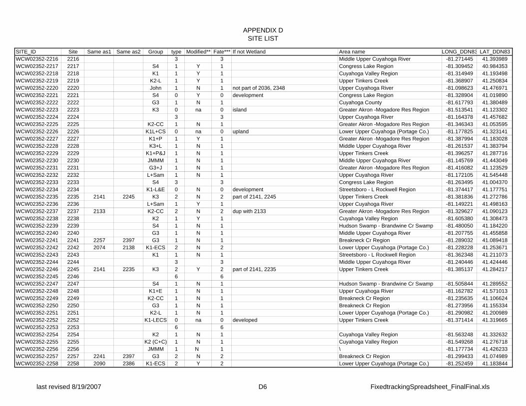
APPENDIX DSITE LIST

SITE_ID Site Same as1 Same as2 Group type Modified** Fate*** If not Wetland Area name LONG_DDN83 LAT_DDN83WCW02352-2216 2216 3 3 Middle Upper Cuyahoga River -81.271445 41.393989WCW02352-2217 2217 S4 1 Y 1 Congress Lake Region -81.309452 40.984353WCW02352-2218 2218 K1 1 Y 1 Cuyahoga Valley Region -81.314949 41.193498WCW02352-2219 2219 K2-L 1 Y 1 Upper Tinkers Creek -81.368907 41.250834WCW02352-2220 2220 John 1 N 1 not part of 2036, 2348 Upper Cuyahoga River -81.098623 41.476971WCW02352-2221 2221 S4 0 Y 0 development Congress Lake Region -81.328904 41.019890WCW02352-2222 2222 G3 1 N 1 Cuyahoga County -81.617793 41.380489WCW02352-2223 2223 K3 0 na 0 island Greater Akron -Mogadore Res Region -81.513541 41.123302WCW02352-2224 2224 3 3 Upper Cuyahoga River -81.164378 41.457682WCW02352-2225 2225 K2-CC 1 N 1 Greater Akron -Mogadore Res Region -81.346343 41.053595WCW02352-2226 2226 K1L+CS 0 na 0 upland Lower Upper Cuyahoga (Portage Co.) -81.177825 41.323141WCW02352-2227 2227 K1+P 1 Y 1 Greater Akron -Mogadore Res Region -81.387994 41.183028WCW02352-2228 2228 K3+L 1 N 1 Middle Upper Cuyahoga River -81.261537 41.383794WCW02352-2229 2229 K1+P&J 1 N 1 Upper Tinkers Creek -81.396257 41.287716WCW02352-2230 2230 JMMM 1 N 1 Middle Upper Cuyahoga River -81.145769 41.443049WCW02352-2231 2231 G3+J 1 N 1 Greater Akron -Mogadore Res Region -81.416082 41.123529WCW02352-2232 2232 L+Sam 1 N 1 Upper Cuyahoga River -81.172105 41.545448WCW02352-2233 2233 S4 3 3 Congress Lake Region -81.263495 41.004370WCW02352-2234 2234 K1-L&E 0 N 0 development Streetsboro - L Rockwell Region -81.374417 41.177751WCW02352-2235 2235 2141 2245 K3 2 N 2 part of 2141, 2245 Upper Tinkers Creek -81.381836 41.272786WCW02352-2236 2236 L+Sam 1 Y 1 Upper Cuyahoga River -81.149221 41.498163WCW02352-2237 2237 2133 K2-CC 2 N 2 dup with 2133 Greater Akron -Mogadore Res Region -81.329627 41.090123WCW02352-2238 2238 K2 1 Y 1 Cuyahoga Valley Region -81.605380 41.308473WCW02352-2239 2239 S4 1 N 1 Hudson Swamp - Brandwine Cr Swamp -81.480050 41.184220WCW02352-2240 2240 G3 1 N 1 Middle Upper Cuyahoga River -81.207755 41.455858WCW02352-2241 2241 2257 2397 G3 1 N 1 Breakneck Cr Region -81.289032 41.089418WCW02352-2242 2242 2074 2138 K1-ECS 2 N 2 Lower Upper Cuyahoga (Portage Co.) -81.228228 41.253671WCW02352-2243 2243 K1 1 N 1 Streetsboro - L Rockwell Region -81.362348 41.211073WCW02352-2244 2244 3 3 Middle Upper Cuyahoga River -81.240446 41.424446WCW02352-2246 2245 2141 2235 K3 2 Y 2 part of 2141, 2235 Upper Tinkers Creek -81.385137 41.284217WCW02352-2245 2246 6 6WCW02352-2247 2247 S4 1 N 1 Hudson Swamp - Brandwine Cr Swamp -81.505844 41.289552WCW02352-2248 2248 K1+E 1 N 1 Upper Cuyahoga River -81.162782 41.571013WCW02352-2249 2249 K2-CC 1 N 1 Breakneck Cr Region -81.235635 41.106624WCW02352-2250 2250 G3 1 N 1 Breakneck Cr Region -81.273956 41.155334WCW02352-2251 2251 K2-L 1 N 1 Lower Upper Cuyahoga (Portage Co.) -81.290982 41.200989WCW02352-2252 2252 K1-LECS 0 na 0 developed Upper Tinkers Creek -81.371414 41.319665WCW02352-2253 2253 6 6WCW02352-2254 2254 K2 1 N 1 Cuyahoga Valley Region -81.563248 41.332632WCW02352-2255 2255 K2 (C+C) 1 N 1 Cuyahoga Valley Region -81.549268 41.276718WCW02352-2256 2256 JMMM 1 N 1 \ -81.177734 41.426233WCW02352-2257 2257 2241 2397 G3 2 N 2 Breakneck Cr Region -81.299433 41.074989WCW02352-2258 2258 2090 2386 K1-ECS 2 Y 2 Lower Upper Cuyahoga (Portage Co.) -81.252459 41.183844

last revised 8/19/2007 D6 FixedtrackingSpreadsheet_FinalFinal.xls

APPENDIX DSITE LIST

SITE_ID Site Same as1 Same as2 Group type Modified** Fate*** If not Wetland Area name LONG_DDN83 LAT_DDN83WCW02352-2259 2259 K1-ECS 3 3 Streetsboro - L Rockwell Region -81.367902 41.190821WCW02352-2260 2260 2092 K1-L+CS 2 N 2 same as 2092 Lower Upper Cuyahoga (Portage Co.) -81.190050 41.348872WCW02352-2261 2261 K3 1 N 1 Upper Tinkers Creek -81.396416 41.311752WCW02352-2262 2262 JMMM 1 N 1 Middle Upper Cuyahoga River -81.163098 41.412896WCW02352-2263 2263 2095 G3 2 N 2 Streetsboro - L Rockwell Region -81.366764 41.127155WCW02352-2264 2264 K1+E 1 N 1 Upper Cuyahoga River -81.141464 41.593036WCW02352-2265 2265 3 3 Congress Lake Region -81.256805 41.038434WCW02352-2266 2266 G3 1 N 1 Breakneck Cr Region -81.315730 41.142214WCW02352-2267 2267 S4 1 N 1 Upper Tinkers Creek -81.431810 41.264012WCW02352-2268 2268 John 1 N 1 Upper Cuyahoga River -81.103718 41.494527WCW02352-2269 2269 G3 1 N 1 Greater Akron -Mogadore Res Region -81.320229 41.104314WCW02352-2270 2270 G3 1 N 1 NOT A DUP, no other points nearby Cuyahoga County -81.696122 41.345388WCW02352-2271 2271 K2 (CC) 0 N 0 house Hudson Swamp - Brandwine Cr Swamp -81.477433 41.226465WCW02352-2272 2272 G3-HS 3 3 Upper Cuyahoga River -81.199078 41.501019WCW02352-2273 2273 3 3 Breakneck Cr Region -81.261398 41.129066WCW02352-2274 2274 K1-LE 0 N 0 fallow field Lower Upper Cuyahoga (Portage Co.) -81.243145 41.318525WCW02352-2275 2275 K1 1 Y 1 Streetsboro - L Rockwell Region -81.316253 41.201838WCW02352-2276 2276 2340 K1-LE 1 N 1 includes 2340 Lower Upper Cuyahoga (Portage Co.) -81.239343 41.335901WCW02352-2277 2277 K3 0 na 0 near canal downtown Greater Akron -Mogadore Res Region -81.517914 41.088244WCW02352-2278 2278 K2(-CS) 0 N 0 farm field Cuyahoga Valley Region -81.583620 41.328422WCW02352-2279 2279 S4 1 Y 1 Cuyahoga Valley Region -81.576638 41.220546WCW02352-2280 2280 K3+L 1 N 1 Middle Upper Cuyahoga River -81.249931 41.426860WCW02352-2281 2281 S4 1 Y 1 Congress Lake Region -81.303891 40.977420WCW02352-2282 2282 G3 1 N 1 Middle Upper Cuyahoga River -81.314039 41.114421WCW02352-2283 2283 Rogers 1 Y 1 need boat Lower Upper Cuyahoga (Portage Co.) -81.304245 41.214037WCW02352-2284 2284 K1-LE 1 N 1 Lower Upper Cuyahoga (Portage Co.) -81.283525 41.329575WCW02352-2285 2285 K2 1 N 1 Cuyahoga Valley Region -81.621188 41.208979WCW02352-2286 2286 G3 1 N 1 Cuyahoga County -81.660677 41.434420WCW02352-2287 2287 K2 1 Y 1 Cuyahoga Valley Region -81.602563 41.157103WCW02352-2288 2288 K3+L 1 N 1 Middle Upper Cuyahoga River -81.244508 41.435229WCW02352-2289 2289 S4 1 N 1 Breakneck Cr Region -81.273087 41.064357WCW02352-2290 2290 JMMM 0 na 0 mature mesic forest Middle Upper Cuyahoga River -81.156161 41.362610WCW02352-2291 2291 K2 1 N 1 Streetsboro - L Rockwell Region -81.392264 41.190864WCW02352-2292 2292 JMMM 1 N 1 Lower Upper Cuyahoga (Portage Co.) -81.167177 41.348894WCW02352-2293 2293 K3+L 1 N 1 Upper Tinkers Creek -81.418099 41.292562WCW02352-2294 2294 G3 1 N 1 Upper Cuyahoga River -81.141480 41.460908WCW02352-2295 2295 K2 1 1 Streetsboro - L Rockwell Region -81.387137 41.110876WCW02352-2296 2296 P+L 0 na 0 ditch Upper Cuyahoga River -81.165966 41.532529WCW02352-2297 2297 S4 3 3 Congress Lake Region -81.268643 41.020701WCW02352-2298 2298 K1-L&E 1 N 1 Streetsboro - L Rockwell Region -81.321917 41.174623WCW02352-2299 2299 Rogers 1 Y 1 Upper Tinkers Creek -81.375788 41.228675WCW02352-2300 2300 3 3 no access Upper Cuyahoga River -81.129307 41.469993WCW02352-2301 2301 2197 K2-CC 2 N 2 dup with 2197 Greater Akron -Mogadore Res Region -81.368620 41.051592

last revised 8/19/2007 D7 FixedtrackingSpreadsheet_FinalFinal.xls

APPENDIX DSITE LIST

SITE_ID Site Same as1 Same as2 Group type Modified** Fate*** If not Wetland Area name LONG_DDN83 LAT_DDN83WCW02352-2302 2302 K2 (-CS) 0 na 0 stream Cuyahoga Valley Region -81.649546 41.328420WCW02352-2303 2303 SF 0 4 photo Hudson Swamp - Brandwine Cr Swamp -81.474790 41.162559WCW02352-2304 2304 G3 1 Y 1 Upper Cuyahoga River -81.178843 41.464342WCW02352-2305 2305 K2-CC 1 N 1 Greater Akron -Mogadore Res Region -81.338069 41.047411WCW02352-2306 2306 K2-CC 1 Y 1 Lower Upper Cuyahoga (Portage Co.) -81.207422 41.297453WCW02352-2307 2307 K2-L 0 na 0 developed Streetsboro - L Rockwell Region -81.357408 41.256744WCW02352-2308 2308 K3+L 1 Y 1 Middle Upper Cuyahoga River -81.235433 41.410146WCW02352-2309 2309 K1-LECS 1 N 1 Upper Tinkers Creek -81.379302 41.313023WCW02352-2310 2310 G3 1 N 1 Upper Cuyahoga River -81.146535 41.457615WCW02352-2311 2311 G3 1 N 1 Greater Akron -Mogadore Res Region -81.396624 41.071215WCW02352-2312 2312 P+L 1 N 1 Upper Cuyahoga River -81.162514 41.549662WCW02352-2313 2313 G3 3 na 3 Breakneck Cr Region -81.263251 41.079491WCW02352-2314 2314 G3 1 N 1 Breakneck Cr Region -81.289720 41.162529WCW02352-2315 2315 K1-ECS 1 Y 1 Lower Upper Cuyahoga (Portage Co.) -81.294164 41.255468WCW02352-2316 2316 G3 1 N 1 Upper Tinkers Creek -81.453642 41.350245WCW02352-2317 2317 6 6WCW02352-2318 2318 S4 1 N 1 Hudson Swamp - Brandwine Cr Swamp -81.526016 41.307724WCW02352-2319 2319 S4 1 Y 1 Cuyahoga Valley Region -81.513467 41.220370WCW02352-2320 2320 G3 3 N 3 couldn't access, poison sumac Middle Upper Cuyahoga River -81.170480 41.446710WCW02352-2321 2321 S4 1 Y 1 Congress Lake Region -81.293729 41.023634WCW02352-2322 2322 K2-L 0 na 0 developed Lower Upper Cuyahoga (Portage Co.) -81.268935 41.230991WCW02352-2323 2323 S4 1 Y 1 Hudson Swamp - Brandwine Cr Swamp -81.456764 41.220474WCW02352-2324 2324 JMMM 1 N 1 Middle Upper Cuyahoga River -81.161607 41.393931WCW02352-2325 2325 K1-LECS 1 N 1 Upper Tinkers Creek -81.395369 41.328844WCW02352-2326 2326 JMMM 1 N 1 Middle Upper Cuyahoga River -81.153265 41.422291WCW02352-2327 2327 K2 1 N 1 Breakneck Cr Region -81.329596 41.127603WCW02352-2328 2328 K1 1 N 1 Upper Cuyahoga River -81.126790 41.576942WCW02352-2329 2329 S4 3 3 Congress Lake Region -81.262228 41.021338WCW02352-2330 2330 K1 1 Y 1 Breakneck Cr Region -81.326070 41.159608WCW02352-2331 2331 S4 3 3 Hudson Swamp - Brandwine Cr Swamp -81.500718 41.278493WCW02352-2332 2332 John 3 3 Upper Cuyahoga River -81.076006 41.544465WCW02352-2333 2333 K2-CC 0 na 0 blackberry bramble Greater Akron -Mogadore Res Region -81.339860 41.076347WCW02352-2334 2334 SF 0 4 photo Cuyahoga County -81.702436 41.458387WCW02352-2335 2335 2007 2119 S4 3 3 denied John Hudson Swamp - Brandwine Cr Swamp -81.483327 41.236784WCW02352-2336 2336 K3CB 0 na 4 photo Middle Upper Cuyahoga River -81.213684 41.360962WCW02352-2337 2337 G3 1 N 1 Breakneck Cr Region -81.236856 41.114131WCW02352-2338 2338 K1-LE 1 N 1 Lower Upper Cuyahoga (Portage Co.) -81.249465 41.320647WCW02352-2339 2339 K1 3 3 Streetsboro - L Rockwell Region -81.328815 41.222564WCW02352-2340 2340 2276 K1-LE 2 N 2 Lower Upper Cuyahoga (Portage Co.) -81.234494 41.331659WCW02352-2341 2341 2117 K3 2 N 2 Greater Akron -Mogadore Res Region -81.405276 41.011131WCW02352-2342 2342 K2 1 N 1 Cuyahoga Valley Region -81.602246 41.322314WCW02352-2343 2343 S4 1 N 1 Cuyahoga Valley Region -81.585032 41.231768WCW02352-2344 2344 K3+L 1 Y 1 Middle Upper Cuyahoga River -81.265588 41.402096

last revised 8/19/2007 D8 FixedtrackingSpreadsheet_FinalFinal.xls

APPENDIX DSITE LIST

SITE_ID Site Same as1 Same as2 Group type Modified** Fate*** If not Wetland Area name LONG_DDN83 LAT_DDN83WCW02352-2345 2345 S4 1 Y 1 Congress Lake Region -81.337898 40.971679WCW02352-2346 2346 K1 1 Y 1 Streetsboro - L Rockwell Region -81.320273 41.185784WCW02352-2347 2347 K2-L 1 N 1 Upper Tinkers Creek -81.377051 41.238983WCW02352-2348 2348 2036 John 2 N 2 part of 2036 Upper Cuyahoga River -81.107439 41.474814WCW02352-2349 2349 K2 1 N 1 Cuyahoga Valley Region -81.626702 41.204217WCW02352-2350 2350 G3 1 N 1 Cuyahoga County -81.609036 41.371632WCW02352-2351 2351 K2 -CC 1 Y 1 Greater Akron -Mogadore Res Region -81.523729 41.144525WCW02352-2352 2352 K3CB 1 Y 1 Middle Upper Cuyahoga River -81.232092 41.440682WCW02352-2353 2353 S4 1 Y 1 Breakneck Cr Region -81.284107 41.056494WCW02352-2354 2354 K1-LE 1 Y 1 Lower Upper Cuyahoga (Portage Co.) -81.195631 41.326701WCW02352-2355 2355 K1 1 N 1 Hudson Swamp - Brandwine Cr Swamp -81.408428 41.216690WCW02352-2356 2356 John 1 N 1 2028, 2108, 2356 all sep assess units jjm Middle Upper Cuyahoga River -81.184734 41.415755WCW02352-2357 2357 3 3 Upper Tinkers Creek -81.434271 41.301128WCW02352-2358 2358 K3 0 na 0 Upper Cuyahoga River -81.109827 41.444903WCW02352-2359 2359 K3 0 na 0 residential pond Greater Akron -Mogadore Res Region -81.456359 41.119398WCW02352-2360 2360 2032 K1 2 N 2 Upper Cuyahoga River -81.174901 41.528192WCW02352-2361 2361 2085 K2 2 N 2 Cuyahoga Valley Region -81.278196 40.984437WCW02352-2362 2362 K1+P 1 N 1 Streetsboro - L Rockwell Region -81.339395 41.183751WCW02352-2363 2363 K2-L 1 Y 1 Upper Tinkers Creek -81.389602 41.261476WCW02352-2364 2364 John 1 N 1 separate point, not part of 2036, 2348 Upper Cuyahoga River -81.095583 41.482897WCW02352-2365 2365 K2-CC 0 N 0 upland lake Greater Akron -Mogadore Res Region -81.368335 41.062261WCW02352-2366 2366 S4 0 na 0 no wetland vegetation Cuyahoga Valley Region -81.621517 41.320041WCW02352-2367 2367 K1-EL 1 Y 1 Hudson Swamp - Brandwine Cr Swamp -81.430797 41.188675WCW02352-2368 2368 G3 0 N 0 Middle Upper Cuyahoga River -81.198662 41.476092WCW02352-2369 2369 G3 1 N 1 Breakneck Cr Region -81.282880 41.107019WCW02352-2370 2370 K1-ECS 1 Y 1 Lower Upper Cuyahoga (Portage Co.) -81.238504 41.242026WCW02352-2371 2371 K1-LECS 1 N 1 Upper Tinkers Creek -81.371264 41.277739

POINTS AFTER 2371 WERE STRANDED OR NOT ASSESSEDWCW02352-2372 2372 7 7 Middle Upper Cuyahoga River -81.239729 41.410857WCW02352-2373 2373 2109 K1+P&J 2 N 8 Upper Tinkers Creek -81.389719 41.291057WCW02352-2374 2374 7 7 Upper Cuyahoga River -81.109436 41.445185WCW02352-2375 2375 K3 8 na 8 upland forest Greater Akron -Mogadore Res Region -81.457800 41.078089WCW02352-2376 2376 7 7 Upper Cuyahoga River -81.163625 41.554116WCW02352-2377 2377 7 7WCW02352-2378 2378 K1-EL 8 N 8 Streetsboro - L Rockwell Region -81.277693 41.173184WCW02352-2379 2379 K1-ECS 8 na 8 camp ground Streetsboro - L Rockwell Region -81.307007 41.258190WCW02352-2380 2380 K1-LECS 8 Y 8 Cuyahoga County -81.439081 41.366090WCW02352-2381 2381 2085 K2 2 N 8 Cuyahoga Valley Region -81.678594 41.130137WCW02352-2382 2382 K1-LECS 8 na 8 Hudson Swamp - Brandwine Cr Swamp -81.491146 41.315620WCW02352-2383 2383 S4 8 N 8 Cuyahoga Valley Region -81.574844 41.292937WCW02352-2384 2384 7 7 Middle Upper Cuyahoga River -81.198962 41.432375WCW02352-2385 2385 S4 8 N 8 Congress Lake Region -81.298502 41.024205WCW02352-2386 2386 2090 2258 K1-ECS 2 N 8 Streetsboro - L Rockwell Region -81.260247 41.182316

last revised 8/19/2007 D9 FixedtrackingSpreadsheet_FinalFinal.xls

APPENDIX DSITE LIST

SITE_ID Site Same as1 Same as2 Group type Modified** Fate*** If not Wetland Area name LONG_DDN83 LAT_DDN83WCW02352-2387 2387 2059 G3+J 2 N 8 Greater Akron -Mogadore Res Region -81.451427 41.150583WCW02352-2388 2388 7 7 Middle Upper Cuyahoga River -81.156705 41.381688WCW02352-2389 2389 2061 K1-LE 8 N 8 Upper Tinkers Creek -81.433153 41.315858WCW02352-2390 2390 7 7 Middle Upper Cuyahoga River -81.162897 41.408012WCW02352-2391 2391 K2 8 N 8 Breakneck Cr Region -81.339733 41.128197WCW02352-2392 2392 7 7 Upper Cuyahoga River -81.086051 41.585870WCW02352-2393 2393 S4 8 Y 8 Congress Lake Region -81.224747 41.041203WCW02352-2394 2394 K1+P 8 na 8 Streetsboro - L Rockwell Region -81.366605 41.163957WCW02352-2395 2395 3 7 major holder says no Upper Tinkers Creek -81.422891 41.258016WCW02352-2396 2396 2068 7 7 Upper Cuyahoga River -81.081865 41.486829WCW02352-2397 2397 2241 2257 G3 2 N 8 Breakneck Cr Region -81.301586 41.084881WCW02352-2398 2398 John 8 N 8 Cuyahoga Valley Region -81.625237 41.268588WCW02352-2399 2399 7 7 Hudson Swamp - Brandwine Cr Swamp -81.473101 41.206572WCW02352-2400 2400 7 7 Upper Cuyahoga River -81.171908 41.512115

41 1317% 5%

Counts Number Percentage0 51 12.8% No wetland found1 217 54.3% Wetlands as 2 18 4.5% Duplicate point3 45 11.3% Access denied4 9 2.3% No wetland based on photo5 26 12.0% Level 3 assessment also completed6 5 Points located outside of Cuyahoga Watershed and Deleted7 12 Points not assessed in first 4008 17 stranded assessed points

Total sites 400 100.0%

Count 0+4 60 15.0% No wetland found (16%)1+5 243 60.8% Wetlands assessed (level 2 + level 3; 66%)

3 45 11.3% Access denied (12%)2 18 5% Duplicate point

37 10.1% No Wetland Found - Map error15 4.1% No Wetland Found - Undetermined8 2.2% No Wetland Found - Filled/Converted

45 12.3% Access Denied18 4.9% Duplicate Point

243 66.4% Wetlands Assessed366

last revised 8/19/2007 D10 FixedtrackingSpreadsheet_FinalFinal.xls