assessment of model risk through hedging simulations...
TRANSCRIPT
Assessment of model risk through hedging simulations:
Valuation of Bermudan swaptions with a one-factorHull-White model
A thesis presented
by
Panayiotis A. Nikolopoulos
to
The Department of Applied Mathematics
in partial ful�llment of the requirements
for the degree of
Master of Science
in the subject of
Applied Mathematics (Financial Engineering Track)
Twente University
Amsterdam, The Netherlands
November 2010

Abstract
In times of globalized �nancial markets, where the complexity of derivative contracts
is severely increasing, the use of advanced models for pricing and hedging is required.
Under this situation, the �nancial institutions desire to quantify the risk and the P&L of
their trading portfolios.
Part of these portfolios consists of contracts with model dependent values. The mod-
els for pricing and risk management are used as an imitation of the actual market evolution
and they are based on various assumptions. The risk management practice considers as a
key factor the quanti�cation of the risk due to the use of a particular model.
This motivates us to investigate the model risk of a popular model within the interest
rate markets, namely the Hull and White short rate model. In this project we will show how
the calibrated Hull and White model affects the hedging outcomes of discrete replicating
strategies on Bermudan swaptions.
Our analysis will allow drawing several conclusions upon the behavior of the model
under mean reversion uncertainty. Finally, we are able to give an estimate of mean reversion
risk using an alternative approach of measurement based on the risk level of the derivative
contract.
Keywords: Model risk, market risk, model reserves, model misspeci�cation, para-
meter uncertainty, model risk measures, model error, error decomposition, discretization,
incomplete markets, hedging, sensitivities, interest rate exotics, swap, swaptions, Bermu-
dan.
iii

Acknowledgments
I want to express my big appreciation to my Professor Arun Bagchi, from Twente
University, for his trust and his support to my master thesis, my master coordinator Profes-
sor Pranab Mandal and my supervisors PhD D.Kandhai, PhD N.Hari from CMRM Quants
Team of ING Group. Drona Kandhai is an Assistant Professor of Computational Finance
at the University of Amsterdam and the Head of Interest Rates Model Validations of ING
Bank. Norbert Hari was a former PhD researcher at Tilburg University and currently works
as a Senior Trading Quantitative Analyst at ING. I personally want to express my acknowl-
edgement to the academic and the professional training that I have been offered from both
Drona and Norbert for the sort period of my internship at the CMRM Trading Quantitative
Analytics of ING. Thanks to them, I am currently discovering new life and career opportu-
nities.
I hope to have the chance to pay you back in the future.
Sincerely, Panos
iv

Contents
Contents . . . . . . . . . . . . . . . . . . . . . . . . . . . . . . . . . . . . . . . . . . . . . . . . . . . . . . . . . . . . . . . . . . . . . . . . . . . . . . . . . v
Preface . . . . . . . . . . . . . . . . . . . . . . . . . . . . . . . . . . . . . . . . . . . . . . . . . . . . . . . . . . . . . . . . . . . . . . . . . . . . . . . . . . . 1
1 Introduction . . . . . . . . . . . . . . . . . . . . . . . . . . . . . . . . . . . . . . . . . . . . . . . . . . . . . . . . . . . . . . . . . . . . . . . . . 3
1.1 Motivation . . . . . . . . . . . . . . . . . . . . . . . . . . . . . . . . . . . . . . . . . . . . . . . . . . . . . . . . . . . . . . . . . . . . . . . . . 3
1.1.1 The problem . . . . . . . . . . . . . . . . . . . . . . . . . . . . . . . . . . . . . . . . . . . . . . . . . . . . . . . . . . . . . . . . 3
1.1.2 Examples . . . . . . . . . . . . . . . . . . . . . . . . . . . . . . . . . . . . . . . . . . . . . . . . . . . . . . . . . . . . . . . . . . . 4
1.1.3 Lessons from the past . . . . . . . . . . . . . . . . . . . . . . . . . . . . . . . . . . . . . . . . . . . . . . . . . . . . . . . . 6
1.2 Objective . . . . . . . . . . . . . . . . . . . . . . . . . . . . . . . . . . . . . . . . . . . . . . . . . . . . . . . . . . . . . . . . . . . . . . . . . . 7
2 Model risk . . . . . . . . . . . . . . . . . . . . . . . . . . . . . . . . . . . . . . . . . . . . . . . . . . . . . . . . . . . . . . . . . . . . . . . . . . . . 8
2.1 De�nition . . . . . . . . . . . . . . . . . . . . . . . . . . . . . . . . . . . . . . . . . . . . . . . . . . . . . . . . . . . . . . . . . . . . . . . . . . 8
2.2 Model risk measures . . . . . . . . . . . . . . . . . . . . . . . . . . . . . . . . . . . . . . . . . . . . . . . . . . . . . . . . . . . . . . . 11
3 Literature survey . . . . . . . . . . . . . . . . . . . . . . . . . . . . . . . . . . . . . . . . . . . . . . . . . . . . . . . . . . . . . . . . . . .15
3.1 First attempt . . . . . . . . . . . . . . . . . . . . . . . . . . . . . . . . . . . . . . . . . . . . . . . . . . . . . . . . . . . . . . . . . . . . . . 15
3.2 Application oriented research . . . . . . . . . . . . . . . . . . . . . . . . . . . . . . . . . . . . . . . . . . . . . . . . . . . . . . 16
3.3 More axiomatic approaches . . . . . . . . . . . . . . . . . . . . . . . . . . . . . . . . . . . . . . . . . . . . . . . . . . . . . . . . 19
3.4 Interest rate markets . . . . . . . . . . . . . . . . . . . . . . . . . . . . . . . . . . . . . . . . . . . . . . . . . . . . . . . . . . . . . . . 21
4 Valuation framework . . . . . . . . . . . . . . . . . . . . . . . . . . . . . . . . . . . . . . . . . . . . . . . . . . . . . . . . . . . . . .24
v

Contents vi
4.1 One factor Hull-White model . . . . . . . . . . . . . . . . . . . . . . . . . . . . . . . . . . . . . . . . . . . . . . . . . . . . . . 24
4.1.1 Term structure . . . . . . . . . . . . . . . . . . . . . . . . . . . . . . . . . . . . . . . . . . . . . . . . . . . . . . . . . . . . . . 25
4.1.2 Volatility structure and mean reversion. . . . . . . . . . . . . . . . . . . . . . . . . . . . . . . . . . . . . . . 27
4.1.3 Calibration . . . . . . . . . . . . . . . . . . . . . . . . . . . . . . . . . . . . . . . . . . . . . . . . . . . . . . . . . . . . . . . . . 29
4.2 Longstaff-Schwartz method . . . . . . . . . . . . . . . . . . . . . . . . . . . . . . . . . . . . . . . . . . . . . . . . . . . . . . . . 30
4.2.1 Valuation algorithm: Least-Square-Method . . . . . . . . . . . . . . . . . . . . . . . . . . . . . . . . . . 31
5 Replication . . . . . . . . . . . . . . . . . . . . . . . . . . . . . . . . . . . . . . . . . . . . . . . . . . . . . . . . . . . . . . . . . . . . . . . . . .34
5.1 Self-�nancing portfolio . . . . . . . . . . . . . . . . . . . . . . . . . . . . . . . . . . . . . . . . . . . . . . . . . . . . . . . . . . . . 35
5.2 Constructing a hedge . . . . . . . . . . . . . . . . . . . . . . . . . . . . . . . . . . . . . . . . . . . . . . . . . . . . . . . . . . . . . . 37
5.3 The idea of replication . . . . . . . . . . . . . . . . . . . . . . . . . . . . . . . . . . . . . . . . . . . . . . . . . . . . . . . . . . . . . 39
5.4 Why forward sensitivities . . . . . . . . . . . . . . . . . . . . . . . . . . . . . . . . . . . . . . . . . . . . . . . . . . . . . . . . . . 40
5.5 A �-neutral portfolio . . . . . . . . . . . . . . . . . . . . . . . . . . . . . . . . . . . . . . . . . . . . . . . . . . . . . . . . . . . . . . 42
5.5.1 A self-�nanced �-hedging portfolio . . . . . . . . . . . . . . . . . . . . . . . . . . . . . . . . . . . . . . . . . 42
5.6 A �V -neutral portfolio . . . . . . . . . . . . . . . . . . . . . . . . . . . . . . . . . . . . . . . . . . . . . . . . . . . . . . . . . . . . 44
5.6.1 A self-�nanced �V -hedging portfolio . . . . . . . . . . . . . . . . . . . . . . . . . . . . . . . . . . . . . . . 45
6 Model risk and related errors . . . . . . . . . . . . . . . . . . . . . . . . . . . . . . . . . . . . . . . . . . . . . . . . . . . .47
6.1 Errors on pricing . . . . . . . . . . . . . . . . . . . . . . . . . . . . . . . . . . . . . . . . . . . . . . . . . . . . . . . . . . . . . . . . . . 47
6.2 Errors on hedging . . . . . . . . . . . . . . . . . . . . . . . . . . . . . . . . . . . . . . . . . . . . . . . . . . . . . . . . . . . . . . . . . 49
6.3 Errors on a �-hedging portfolio . . . . . . . . . . . . . . . . . . . . . . . . . . . . . . . . . . . . . . . . . . . . . . . . . . . . 50
6.4 Errors - Market risk - Model risk . . . . . . . . . . . . . . . . . . . . . . . . . . . . . . . . . . . . . . . . . . . . . . . . . . . 53
7 Results I: Hedge test . . . . . . . . . . . . . . . . . . . . . . . . . . . . . . . . . . . . . . . . . . . . . . . . . . . . . . . . . . . . . . .55
7.1 Historical data . . . . . . . . . . . . . . . . . . . . . . . . . . . . . . . . . . . . . . . . . . . . . . . . . . . . . . . . . . . . . . . . . . . . 55

Contents vii
7.2 Validation strategy. . . . . . . . . . . . . . . . . . . . . . . . . . . . . . . . . . . . . . . . . . . . . . . . . . . . . . . . . . . . . . . . . 57
7.3 Results . . . . . . . . . . . . . . . . . . . . . . . . . . . . . . . . . . . . . . . . . . . . . . . . . . . . . . . . . . . . . . . . . . . . . . . . . . . 58
7.3.1 Vanilla swaps . . . . . . . . . . . . . . . . . . . . . . . . . . . . . . . . . . . . . . . . . . . . . . . . . . . . . . . . . . . . . . 59
7.3.2 Vanilla swaptions . . . . . . . . . . . . . . . . . . . . . . . . . . . . . . . . . . . . . . . . . . . . . . . . . . . . . . . . . . . 60
7.4 Evaluation of hedging performance. . . . . . . . . . . . . . . . . . . . . . . . . . . . . . . . . . . . . . . . . . . . . . . . . 64
7.4.1 Decomposition of hedging errors: Evidence . . . . . . . . . . . . . . . . . . . . . . . . . . . . . . . . . . 64
7.4.2 Forward vs Spot sensitivities: Robustness . . . . . . . . . . . . . . . . . . . . . . . . . . . . . . . . . . . . 65
7.4.3 Hedging frequency . . . . . . . . . . . . . . . . . . . . . . . . . . . . . . . . . . . . . . . . . . . . . . . . . . . . . . . . . 67
7.4.4 Bumping size: The effect of second-order risks . . . . . . . . . . . . . . . . . . . . . . . . . . . . . . 69
7.5 Model risk: The vanilla case . . . . . . . . . . . . . . . . . . . . . . . . . . . . . . . . . . . . . . . . . . . . . . . . . . . . . . . 71
8 Results II: Model risk assessment . . . . . . . . . . . . . . . . . . . . . . . . . . . . . . . . . . . . . . . . . . . . . . . .73
8.1 Methodology . . . . . . . . . . . . . . . . . . . . . . . . . . . . . . . . . . . . . . . . . . . . . . . . . . . . . . . . . . . . . . . . . . . . . . 74
8.1.1 De�nition of experiments . . . . . . . . . . . . . . . . . . . . . . . . . . . . . . . . . . . . . . . . . . . . . . . . . . . 75
8.1.2 Collection of results: Observed characteristics . . . . . . . . . . . . . . . . . . . . . . . . . . . . . . . 76
8.1.3 Data analysis . . . . . . . . . . . . . . . . . . . . . . . . . . . . . . . . . . . . . . . . . . . . . . . . . . . . . . . . . . . . . . . 77
8.2 Hedge test results: 5 year Bermudan swaption . . . . . . . . . . . . . . . . . . . . . . . . . . . . . . . . . . . . . . 78
8.2.1 High vega risk deals . . . . . . . . . . . . . . . . . . . . . . . . . . . . . . . . . . . . . . . . . . . . . . . . . . . . . . . . 80
8.2.2 Low vega risk deals . . . . . . . . . . . . . . . . . . . . . . . . . . . . . . . . . . . . . . . . . . . . . . . . . . . . . . . . . 83
8.2.3 Analysis of observed data . . . . . . . . . . . . . . . . . . . . . . . . . . . . . . . . . . . . . . . . . . . . . . . . . . . 86
8.3 Hedge test results: 20 year Bermudan swaption . . . . . . . . . . . . . . . . . . . . . . . . . . . . . . . . . . . . . 90
8.3.1 High model risk deals . . . . . . . . . . . . . . . . . . . . . . . . . . . . . . . . . . . . . . . . . . . . . . . . . . . . . . . 91
8.3.2 Analysis of observed data . . . . . . . . . . . . . . . . . . . . . . . . . . . . . . . . . . . . . . . . . . . . . . . . . . . 92
8.4 An estimate for model risk . . . . . . . . . . . . . . . . . . . . . . . . . . . . . . . . . . . . . . . . . . . . . . . . . . . . . . . . . 95

Contents viii
9 Conclusion . . . . . . . . . . . . . . . . . . . . . . . . . . . . . . . . . . . . . . . . . . . . . . . . . . . . . . . . . . . . . . . . . . . . . . . . . .98
9.1 Project evaluation . . . . . . . . . . . . . . . . . . . . . . . . . . . . . . . . . . . . . . . . . . . . . . . . . . . . . . . . . . . . . . . . . 98
9.2 Future work . . . . . . . . . . . . . . . . . . . . . . . . . . . . . . . . . . . . . . . . . . . . . . . . . . . . . . . . . . . . . . . . . . . . . . 100
References . . . . . . . . . . . . . . . . . . . . . . . . . . . . . . . . . . . . . . . . . . . . . . . . . . . . . . . . . . . . . . . . . . . . . . . . . . . 102
A Af�ne modeling . . . . . . . . . . . . . . . . . . . . . . . . . . . . . . . . . . . . . . . . . . . . . . . . . . . . . . . . . . . . . . . . . . . 107
B Piecewise constant volatility . . . . . . . . . . . . . . . . . . . . . . . . . . . . . . . . . . . . . . . . . . . . . . . . . . . . 109
C Plotting functions . . . . . . . . . . . . . . . . . . . . . . . . . . . . . . . . . . . . . . . . . . . . . . . . . . . . . . . . . . . . . . . . 112
D Results: The effect of mean reversion . . . . . . . . . . . . . . . . . . . . . . . . . . . . . . . . . . . . . . . . . 114
E Results: The effect of moneyness . . . . . . . . . . . . . . . . . . . . . . . . . . . . . . . . . . . . . . . . . . . . . . . 116
F Results: The effect of market risk . . . . . . . . . . . . . . . . . . . . . . . . . . . . . . . . . . . . . . . . . . . . . 118
G Results: High and low risk deals . . . . . . . . . . . . . . . . . . . . . . . . . . . . . . . . . . . . . . . . . . . . . . . 120
H Tables: Initial price & Final hedging error . . . . . . . . . . . . . . . . . . . . . . . . . . . . . . . . . . . 123

Preface
This document has been designed to offer a useful insight on a very important aspect of quan-
titative �nance and risk management, namely the quanti�cation of model risk. The text targets on
�nal year master students of �nancial mathematics and market practitioners with some knowledge
of derivatives pricing.
Chapter 1 starts with an overview of the problem and states the main objectives of this
project. In chapter 2 the formal de�nition of model risk follows. Chapter 3 is a brief survey
of previous researches on the topic starting from 1989 up to now. This chapter aims to give a gen-
eral picture about how other people interpret model risk and how they have tried to extract it from
the given information without getting into much details.
A full documentation is provided for the implementation of the examined short rate model
and how the replicating strategies are de�ned on the hedge test module on chapters 4 and 5 respec-
tively. After a signi�cant empirical exposure with the subject we �nd the need of describing model
risk as it is observed in the experimental outcomes of the hedge tests. For that reason, chapter 6
presents our interpretation on model risk and its related errors. Our understanding has been in-
�uenced by ideas from the literature and from our experimental knowledge. This description will
help the reader to understand the results that follow next.
The �rst part of the results, chapter 7, is dedicated on the validation of our hedger module by
testing its performance on different interest rate vanilla payoffs. Taking advantage of the simplicity
of these payoffs several tasks like hedging frequency, type of sensitivities, decomposition of errors
and other are being investigated. Chapter 8 presents the main results of this project, the hedge tests
1
Preface 2
of Bermudan swaptions. Finally we conclude on the experimental evidences and the results of
their analysis. At the end we summarize and we address potential directions for the quanti�cation
of model risk.
Panos Nikolopoulos
Amsterdam, November 2010
Chapter 1Introduction
1.1 Motivation
1.1.1 The problem
Nowadays, we witness an increasing complexity of the �nancial derivatives being traded in the
market. For this reason it is essential to use sophisticated models for pricing and risk management.
The subject of model risk is related to the inaccurate valuation and hedging by a certain model.
For liquid instruments this risk can be obtained from the difference between the market and model
price. Nevertheless in this text, our interest is focused on more exotic trades where no market price
is available and the hedging portfolio plays an important role on the product value. This is because
the fair derivative price should represent the total cost of its replicating strategy.
So far, it is well understood that perfect replication by any self-�nancing strategy is only pos-
sible in complete markets with no transaction costs and continuous hedging. In case of incomplete
markets our replicating portfolio is no longer risk-free and is subjected to market risk. Market
risk appears as an extra cost on the hedging portfolio due to changes of market factors like in-
terest rates, volatilities etc. In order to allocate the amount of capital for the exposure of issuing
new products one needs to calculate some risk measures using a variety of models and techniques.
These measures can be computed as soon as we choose a model to describe the evolution of the
underlying factors and for this, simulation is necessary.
3

1.1 Motivation 4
Historically, model simulations have been used for testing trading strategies since 1977 start-
ing with Galai and followed by Merton & Scholes [1978] and Gladstein [1982]. With simulations
we can imitate the behavior, for instance, of the term structure of interest rates or the volatility sur-
face of options prices or any other stochastic market variable. In this way, it is possible to generate
a class of scenarios from which a Pro�t-Loss (P&L) distribution is created for the trading portfo-
lio. In risk management practice, people are mainly interested in the probability of extreme losses
and this can be quanti�ed by using several market risk measures like VaR or Expected Shortfall
(see Basel Committee regulations [1999]). Unfortunately, all models are based on assumptions and
they are simply approximations of the actual dynamics (see Derman [1996] and Rebonato [2001]).
In reality we are not able to capture the "real" generating process and that makes both pricing and
hedging model sensitive. In order to illustrate this in more detail we will try to describe it through
three simple examples.
1.1.2 Examples
Consider the well-known pricing model of Black-Scholes (BS) [1973]. The BS model assumes
that the underlying asset follows a lognormal diffusion process. However, this model underesti-
mates the probability of high increments, while the practice shows that the tails of the empirical
distribution can be more extreme than those of a lognormal distribution. In other words, a stan-
dard valuation model may be misspeci�ed when it is based on speci�c distributional assumptions
which are not supported by the actual �nancial markets.
Moreover, consider a European call on a stock while the underlying follows a lognormal
process. Then, a model like Black-Scholes would be a reasonable choice for pricing. However,
1.1 Motivation 5
the model assumes constant volatility which in reality is not correct. Traders try to correct this
assumption by calibrating the model to input data in order to imply the volatility for the current
day. Calibration is a numerical method which depends on the quality of the market data. Due to this
fact, the implied parameter can be higher or lower than the real volatility of the call option. This
inevitably will lead to pricing and hedging errors. The parameter speci�cation therefore will be an
additional source of risk, even if the model satis�es the distributional behavior of the underlying.
Another example which is more related to the current �nancial situation is the introduction
of counterparty risk value adjustment (CVA) to pricing since the beginning of the recent crisis.
Suppose that before that period the pricing of a �nancial derivative would require the use of one
interest rate curve. After the crisis, the establishment of CVA on pricing requires at least two
interest rate curves, one for discounting and one for the calculation of the forward rates. That
means that if the market prices of those products were driven by a one-factor model before the
summer of 2007, the current market prices might behave at least as a two-factor model.
Taking into account the previous example, assume that we are able to successfully approx-
imate the real model process with a highly consistent model to market prices. Suppose that the
model shows remarkable performance for the last ten years. Next, imagine that today a product,
maturing at three years from now, is priced with this model. However, six months after the issuing
date something happens and the market prices start behaving as a different process. That means
that the product price may be completely different than what was initially expected from the issuer.
If this new market process belongs to the set of our known models then the risk can be seen within
the range of all model prices. If the opposite happens, meaning that the new market price is out of
the known price range, we are facing a high risk. This is because our current market knowledge

1.1 Motivation 6
does not allow us to identify such a process much earlier. Therefore, model risk can be completely
unexpected even when one uses the most accurate models of its time.
In a competitive market, related situations of model uncertainty can bring huge losses to the
option issuer. Because of similar reasons the world of �nance has experienced several embarrassing
incidents due to wrong or inadequate models for the last twenty years.
1.1.3 Lessons from the past
In the past we have seen cases of big losses due to the use of derivative products even for simple
underlyings such as bonds or stocks. Some well known examples are those of Barings, Metallge-
sellschaft, Procter & Gamble, Orange County, Showa Oil, Gibson Greetings or Long Term Capital
Management. More speci�cally, in 1997, the Bank of Tokyo-Mitsubishi announced that its New
York-based derivatives unit was taking an $83 million after-tax write-off because a computer model
overvalued a portfolio of swaps and options on USD interest rates.
The same year, many derivatives traders noted that NatWest Markets, one of the largest banks
in the UK, was aggressively pricing interest rate options and swaptions. It is believed that their
valuation was ignoring the effect of volatility smile in its OTC swaptions prices with different mon-
eyness on Sterling/German mark. The failure of the bank's pricing and risk management models to
incorporate the "volatility smile" effect led to a signi�cant over-valuation of the portfolio. Losses
from these trades eventually totaled £90 million. People speculate that this may have occurred for
a total period of three years.
1.2 Objective 7
These are only few examples, where model risk was the reason of big losses. Cases like
those attract our interest to study a series of different deals and models in a wide range of historical
market scenarios.
1.2 Objective
With this in mind, our project aims to assess the exposure of pricing and hedging interest rate ex-
otics by the one-factor Hull and White short rate model. Our experiments will focus on Bermudan
swaptions for which very limited information has been reported in the literature (see chapter 3).
The assessment of model risk will be based on the study of hedging simulations and the analysis
of their �nal hedging outcomes.
The �rst task of our analysis is to describe model risk and its related errors on pricing and
hedging (see chapter 6). The description will be in�uenced from ideas in the literature and our
experimental experience. In order to gain hedging experience we will need to create a big variety
of hedge tests, for several interest rate vanilla products (see chapter 7), and analyze the related
hedging errors.
The last part of this research will concentrate on the extensive analysis of the hedging results.
Our interest is to learn how and which values are affected from the mean reversion risk. The �nal
goal of the project is to estimate model risk (see chapter 8) based on a set of arti�cial experiments
and identify a possible direction that can lead to a sound model risk quanti�cation in the future.

Chapter 2Model risk
The point of option pricing theory is usually the speci�cation of a stochastic model and a
set of future scenarios (;F) with a probability measure P de�ned on these outcomes. There are
many cases in �nancial decision making where the decision maker is not able to assign an exact
probability to the future outcomes. Such measures describe the odds of a �nancial pricing rule (or
model). The dif�culty of de�ning a risk-averse pricing rule attracts the interest of both practitioners
and academics and it is the main problem of model risk.
The �rst section of this chapter provides a philosophical description of model risk using
de�nitions from the literature. The second section de�nes three model risk measures that have
been proposed for model risk quanti�cation in previous researches.
2.1 De�nition
Consider a sample space of all possible market scenarios. Ft is a collection of subsets of
which represents all the market information until time t. Because there is no reference probability
measure on , we de�ne an objective probability measure P on the set of all market scenarios
(;Ft). That means P describes the objective probabilities of market evolution. We also de�ne
an Ft-measurable process fStgTt=0 which is a mapping of the form St : ! R. Moreover, if
there exists another probability measure Qm on (;Ft) such that St is a martingale under Qm,
we can create an arbitrage-free pricing rule on that space. In other words, Qm, describes the risk
8
2.1 De�nition 9
neutral probabilities ofm pricing model and it is uniquely de�ned in a complete market ( see Bjork
[2004]).
However, there is always an uncertainty on de�ning such measures. In complete markets the
uncertainty on Qm depends only on the lack of identi�cation (read p.11 for more details) of the
measure P due the limitation to historical data. On the other hand, in incomplete markets even if
we are certain about P, Qm is no longer unique. Hence, there is an ambiguity of choosing a risk
neutral probability measure to describe the future outcomes.
De�nition 1 Risk is the uncertainty over the future outcomes, while we are able to specify a
unique probability measure.
De�nition 2 Ambiguity (Knightian uncertainty) is the uncertainty over the choice of the right
probability measure.
The message from this setting is that under ambiguity we cannot condition neither the hedg-
ing strategy nor the derivative price on a �xed model. In that sense we do not know what is the
unique fair price or what is the unique distribution of the hedging errors. Below, we present model
risk as it is appeared in the literature and several methodologies to quantify it. For that reason, we
will need to consider that there exists a class of models K, such that a risk-neutral model m 2 K
is de�ned on a probability space (m;Fm;Qm).
Model risk: general de�nition
�The risk associated to the mismatch between the model dynamics and the actual dynamics is
called model risk�, Kerkhof [2002]. �Model risk is the risk of occurrence of a signi�cant difference
2.1 De�nition 10
between the mark-to-model value of a complex and/or illiquid instrument, and the price at which
the same instrument is revealed to have traded in the market.� Rebonato [2004].
Model risk is the exposure to �nancial losses due to misspeci�ed or incorrectly applied
model. In case of risk management, we can interpret model risk as the cost of our hedging strategy
additionally to the cost of market risk which is represented on our P&L distribution. The cost of
model risk arises due to the inaccurate generation of the P&L distribution. Under this framework
of pricing models, the model risk can be decomposed to the following categories (see Kerkhof
[2010]).
Estimation risk
Suppose the true modelm(#) 2 K is known, with # a structural parameter ofm. If^#0 is the
optimal estimate of # for the current market data, the risk of calculating a price using m(^#i) with
i 6= 0 is called estimation risk. This source of risk depends on the quality and liquidity of the input
data and the robustness of the optimization process.
Misspeci�cation risk
Consider a class of models K. Assume that the price of the true model is within the range
of all model prices of class K, nevertheless the real model may not be available in class K. The
valuation by any model m 2 K will probably deviate around the real price. The uncertainty of
pricing or hedging with a wrong modelm is usually called misspeci�cation risk.

2.2 Model risk measures 11
Identi�cation risk
In order to model a physical or a �nancial process �rst we need to observe its behavior. For
instance, we can identify the drift, the density of its increments, mean reversion characteristics or
whatsoever. Then we can try to replicate this behavior by de�ning a stochastic process with the
same (or similar) characteristics. In practice, we are only able to observe the past. As a result
theoretically we can only de�ne a highly speci�ed1 model for our historical data. In �nance, nev-
ertheless, the market in driven by the human factor and not from physical laws. As a consequence
the market process may change its behavior (model) at a certain point in the future. Since the future
data are not known, it is impossible to identify the real process, hence it is impossible to replicate
its behavior. This is called, from Kerkhof [2010], identi�cation risk. This is the risk of identi-
�ng the market process based only on previous market data. Under this situation it is not easy to
measure model risk by any of the available methods. However, the literature proposes some mea-
surements methods regarding the �rst two categories which we are going to analyze on the next
section.
2.2 Model risk measures
Suppose that we have a T -claim X and the price of its replicating portfolio is given by �(T ;X )
at time T . Then we denote as D = X��(T ;X ) as the premium of market and model risk that
need to be added to the price of our portfolio to meet the �nal condition of claim X . This can be
interpreted as the capital that somebody would need to keep as a protection frommodel uncertainty.
1 Speci�ed model is a highly accurate stochastic process which successfully can replicate the observed data.

2.2 Model risk measures 12
Worst-case measure
Giboa&Schmeidler [1989] started the foundation of this approach and several strategies have
been presented on the papers of Kirch [2002], Föllmer&Schied [2002] and Kerkhof [2002]. This
approach gives an upper bound for the model risk of the T -claim X . The formal de�nition is given
by Kerkhof [2002].
Consider a class C of all possible models and a model m which is an element of C. Let also
K � C a subset of the initial class with m 2 K. We will call K a tolerance set and m nominal
model. Suppose that we have a product � which is de�ned on the class C and the model risk
measure is de�ned on class K. Then the worst-scenario measure for model risk is de�ned under
some probability measure P, while P is based on the current statistical knowledge of the market
process:
�P(�;m;K) = supk2KUk(�k)� Um(�m)
where �k is the price of the portfolio with respect to k and Uk is the risk management method to
assess the pro�t or loss of the hedging portfolio.
MaxMin measure
An alternative method to that of the worst-case approach is to calculate a "MaxMin" measure
which is the range of all model prices within the set K. This measure has been proposed by Cont
[2006] and does not depend on the choice of the nominal model. This measure is de�ned as follows
�P(�;m; l;K) = supk2KUk(�k)� inf
l2KUl(�l)

2.2 Model risk measures 13
Bayesian measure
This approach was �rst introduced by Hoeting [1999]. The model risk measure is a weighted
average of risk measures. A �nancial institution can give less weight to those models when it is
believed that they are more risky than others.
Consider again the set K = fm1;m2; :::;mNg with the candidates models. Let us suppose
that these models have parameters #i 2 Ei for i = f1; 2; :::; Ng.Then, the density that represents
our view about the model parameters #i conditionally that the model mi holds can be denoted as
p(#ijmi). Moreover, the �nancial institution may set the model probabilities P(mi) according to
its experience for the actual model.
The weights that a �nancial institution assigns to each model can be expressed as probabili-
ties, based on the Bayes rule for a set of historical observations B. Then, p(Bjmi) is a likelihood
integral of the data under the modelmk,
p(Bjmk) =
ZEi
p(#kjmk)P(Bj#k;mk)d#k
and the probability for a modelmk;, given a set of observations B, is
P(mkjB) =P(mk \B)P(B)
=p(Bjmk)P(mk)PNi=1 p(Bjmi)P(mi)
The main idea of this approach is that if we want to compute the moment of a random variable
X under model uncertainty, we can use the set of observations B and the conditional probabilities
that this set indicates. The approximation of the moments of X is a weighted average of all the
moments with respect to a certain model. For example the �rst moment of X given by B is
E[XjB] =NXi=1
E[Xjmi; B]P(mijB)

2.2 Model risk measures 14
The expectation, �nally, will represent the nominal price of variableX . Once, the nominal price is
de�ned measurements can be applied.
Bayesian vs. Worst-case approach
A known disadvantage of the worst-case measure is the dif�culty to create the set of the
candidate models. An even more dif�cult task, though, is to de�ne the nominal modelm 2 K. The
MaxMin measure overcomes this obstacle but it becomes more conservative to quantify model risk
and more expensive in a competitive market. The choice of nominal model is also not a problem for
the Bayesian approach (see Bragner&Schlag [2004]). Nonetheless, the Bayesian measure does not
assume that the actual model belongs to the set of candidate models. The main idea of this method
is to assign small probability to unfavorable models without making implicit assumption on the true
model. In that sense, it is hard and sort of arbitrary to decide which model is more signi�cant than
the other. This makes the Bayesian approach dif�cult to implement from a practical point of view
(see Cont [2006] and Kerkhof [2010]). In practice we need to have a strong knowledge about the
models and big experience according to previous market data in order to assign reasonable weights
to each model. Limited data or the possibility of poor understanding of the real data process could
be too risky for the Bayesian measure.
On the following chapter we provide a quick summary of twenty years of research on the
topic. In this summary, several trials of extracting model risk out of the observed prices are listed.

Chapter 3Literature survey
In this chapter we present a brief overview of previous researches on model risk and we
discuss their impact on derivatives pricing and hedging. The purpose of this survey is to get a
general idea of how people tried to extract or study model risk without getting into unnecessary
details. In this chapter we identify three different patterns of available information. The �rst group
is application-oriented papers, the second is about more general and axiomatic approaches and the
last group focuses on the model uncertainty in incomplete and especially in interest rate markets.
3.1 First attempt
Looking back retrospectively at 1983 we found the �rst attempt of investigating model risk by
Galai. In his paper the author tries to decompose the returns of the hedging strategies due to
discretization and due to the model choice. The decomposition of model error is based on nothing
else than comparing actual and model prices derived from plain vanilla equity options. The
difference between the current and previous prices is considered to be the discretization effect
of the strategy. In order to get the relevant error terms, the differences are applied either on the
derivative or on the hedging portfolio price. For the experimental scenarios historical data are
used. A daily hedging based on Black-Scholes (BS) model is implemented for European equity
call options traded on CBOE. The results indicate that the contribution of the model error plays an
important role on determining the prices.
15

3.2 Application oriented research 16
3.2 Application oriented research
Bakshi, Cao and Chen [1997] compare the pricing and hedging performance, of vanilla equity
call options from S&P500. In this paper it is examined how the Black-Scholes model performs
against models that combine stochastic volatility(SV), stochastic interest(SI) and random jumps(J).
The assessment of model misspeci�cation is based on comparing implied volatility graphs of dif-
ferent models, across different moneyness and time to maturity (see Rubinstein [1985]), and by
checking the consistency of implied volatility given from one model (see Bates [1996]) compared
to this observed from the market data. The experiment involves estimating the model parameters
from sample data and then testing the process out of sample. The results indicate better perfor-
mance for SV model, however SV, SVJ, SVSI models are signi�cantly misspeci�ed in terms of
internal consistency. Random jumps seem to improve the pricing of short-term options; whereas
modeling stochastic interest rates, the random jumps can enhance the �t of long-term options.
Green&Figlewski [1999] have shown how to minimize the risk of derivative's position by
dynamic hedging strategies in presence of model risk for equity, FX, interest rate vanilla products.
The experiments are using historical scenarios taken from S&P500 and other important markets.
The research considers hedging through diversi�cation across different markets, cash �ow match-
ing and delta hedging. The risk of these trading strategies is examined for standard European puts
and calls that are valued with some appropriate form of Black-Scholes model. The volatility input
for the BS model is forecasted from the historical data either as an unconditional standard devia-
tion or as an exponential weighted deviation. The impact on the deviation of the prices of these
trading strategies is examined for non-optimal volatility parameters and different money-
3.2 Application oriented research 17
ness. The results conclude that delta hedging is the most reasonable hedging strategy when the
volatility is optimally estimated from the historical data.
Jiang&Oomen [2001], two years later, have discussed the impact of model misspeci�cation
on hedging. The authors claim that the magnitude of model risk can be isolated by comparing
the performance of hedging based on a wrong or misspeci�ed model to those based on cor-
rectly speci�ed models. This argument is based on the idea of Bakshi, Cao & Chen [1997] to
answer the question �Which is the least misspeci�ed model?�. For instance the SVSI-J (stochas-
tic volatility, stochastic interest, stochastic jump) model which combines all the extensions of BS
model outperforms the models which are missing one of these characteristics with respect to pric-
ing error and hedging. In this spirit, Jiang & Oomen examine the performance of different hedging
strategies varies across different pricing models, option's moneyness, option's maturity and by per-
forming delta-vega-(rho) hedging strategies on European call options. They apply their method to
examine the performance of volatility options and how the risk factors ( interest, volatility, asset
returns, etc.) can be hedged with certain strategies. Regarding the input values for the interest rate,
the simulation results show that the choice between the market implied and model implied val-
ues has a very small impact on the hedging performance. However, when the stochastic interest
rate is considered as constant the impact on the hedging effectiveness of ATM options, especially
for medium- and long-term options is signi�cant. Finally the research shows that the most impor-
tant factor which affects the hedging performance under model misspeci�cation is the input for the
volatility parameter.
One year later, Hull&Suo [2002] investigate a method to quantify the exposure due to model
risk for illiquid exotics. They propose the following approach: Assume that prices in the market

3.2 Application oriented research 18
are governed by a plausible multi-factor no-arbitrage model, the so called �true model� (see
Bakshi, Cao & Chen [1997]), that is a lot more different and complex than the model being tested.
In this paper the model risk of CR-IVFmodel (continuously recalibrated - implied volatility model)
is examined by continuously �tting the �true model�, a two-factor stochastic volatility model to
market data (for more details see Schöbel and Zhu [1998]). Thereafter, the prices of compound and
barrier options, given from the stochastic model, are compared to those that are priced under the
Black-Scholes assumptions using the implied volatility taken from the CR-IVF formula. Hull&Suo
�nd that the CR-IVF model gives reasonably good results for compound options while the results
for barrier options are much less satisfactory. This indicates that barrier option more sensitive to
path dependence than the compound options and that the size of model error is positively correlated
to the number of payoff dates.
In the same period, Kerkhof, Melenberg & Schumacher [2002], have tried to assess the total
hedging error instead of simply calculating hedging ratios. Since the actual dynamics are not avail-
able historical data simulation is applied, and following the steps proposed by Hull&Suo [2002] a
benchmark model is de�ned. They investigate OTM, ATM, ITM European call options according
to dividend paying Black-Scholes model for FX and S&P500 options. The total model risk is de-
composed in model risk due to estimation error and model risk due to misspeci�cation. The
estimation risk is calculated by testing one model for different input parameters and the misspec-
i�cation risk for a set of different models. The research applies the worst-case measure for the
quanti�cation and it stresses that the misspeci�cation risk dominates the estimation risk. It is also
shown that the nonparametric estimates of the P&L distribution, under the model assumptions, are
more or less symmetric while the empirical density is skewed to the left. This explains why it hap-
3.3 More axiomatic approaches 19
pens more often than expected that the actual cost of hedging exceeds the option premium by a
substantial amount.
3.3 More axiomatic approaches
After a couple of years we �nd researchers trying to move from application-oriented papers to more
general and axiomatic approaches for model risk. Branger&Schlag [2004] emphasize that before
doing hedging simulations it is essential to choose a robust market risk measure and an optimally
minimized hedging strategy which should be model insensitive in order to come up with a solid
ground for model risk assessment. They examine a naive, the worst case and the Bayesian approach
for model risk quanti�cation. The authors stress that the aggregated risk is very important for the
optimization of the hedging strategy and they believe that the Bayesian method is more appropriate
to aggregate the market and model risk (see chapter 2 for the de�nition and the dif�culties of this
approach).
As model risk attracts more attention from the research community, in 2006, an interest-
ing work by Cont comes to light. In this paper the author tries to distinguish the uncertainty of
econometric estimation from the uncertainty of risk neutral models and he presents a number of
properties2 for model risk assessment. According to these properties a coherent3 measure is de�ned
for model risk, as the range of all candidate model prices, while models are marked-to-market.
The applicability of the measure is studied for European options priced with the Black-Scholes
2 Properties that have already been addressed on previous papers like liquidity of benchmark instruments, model-freereplicating strategies, the risk of static hedging, the risk of market prices, etc.3 A measure de�ned by Artzner [1999], which satis�es the properties of monotonicity, sub-additivity, translationinvariance and positive homogenuity (see also Frey [2005])
3.3 More axiomatic approaches 20
(BS) model under local volatility uncertainty and for static hedging strategies. In one of the exam-
ples where a barrier option is priced with a local volatility model and a BS model with jumps the
measurement shows that model risk composes the 40% of the derivatives selling price. In addition
to that, an alternative measure is proposed which does not require model calibration. In order to
achieve this Cont introduces a convex4 measure which takes as an adjustment the difference norm
between the model and market price along the set of benchmark instruments. Then the model risk
is de�ned as the range of all these convex measures that correspond to the set of all candidate
models. For more details we refer to [53].
In the beginning of the current year, Kerkhof, Melenberg&Schumacher [2010] publish a
paper which incorporates model risk into risk measure calculations using classes of models based
on standard econometric methods. This work continues on the same spirit as the paper of [2002],
while it tries to incorporate the new concepts of ambiguity and lack of identi�cation (see chapter
[2] for more details). In that sense an new type of uncertainty is de�ned, the identi�cation risk. The
quanti�cation of model risk, is achieved on top of market risk, by using the worst-case approach
to measure the aggregated total risk. By using this measurement the nominal risk measure, such as
VaR or Expected Shortfall, is adjusted accordingly. In this way market risk is estimated using a
class of models and not only one particular model. The method is applied on S&P500 and FX
data and the analysis is done by using a rolling window of two years for a range of historical data.
4 A measure de�ned by Föllmer and Schied [2002], which relaxes the property of positive homogenuity to �(�X +(1 � �)Y ) = ��(X) + (1 � �)�(Y ) , 8� 2 [0; 1]. Where X and Y represent the payoff of an option or portfolio.This measure can be de�ned as �(X) = sup
Q2K
�EQ [X]� � (Q)
instead of the classic worst-case form �(X) =
supQ2K
�EQ [X]
. Q is the risk neutral measure, K is the set of candidate models and � (Q) is a penalty function ( see
Cont [2006] ), which is the measure's adjustment to the systematic mispricing of the benchmark instruments by thecorresponding model.
3.4 Interest rate markets 21
3.4 Interest rate markets
Bossy, Gibson, Lhabitant, Pistre &Talay [2007], in the same spirit as in [2000] and [2001], have
developed a conceptual framework for decomposing the P&L related to model misspeci�cation
for interest rate claims. For this, an analytical way is proposed to decompose P&L to initial pric-
ing error, model pricing error at any time and the cumulative risk due to hedging error. They inves-
tigate the sensitivity of forward P&L with respect to volatility, forward yield curve and frequency
of rebalancing for bond options. The research is restricted to model risk assessment of Markovian
univariate HJM and short rate models (Ho-Lee, Vasicek, CIR) but the underlying methodology can
be applied to a larger class of hedging strategies with univariate Markov models. The results, like
those of Figlewski&Green [1999], suggest that the discreteness of the replicating portfolio mag-
ni�es model risk, even for short rebalancing time intervals. The paper leaves to a future work the
assessment of the hedging strategy when higher order multi-factor models are used.
Furthermore, there are few other noticeable papers related to the interest rate market which
we will mention below without going much into detail. There are two similar approaches like
that of Hull&Suo [2002] namely the work of Longstaff, Santa-Clara & Schwartz [2001] and An-
dersen&Andreasen [2001]. These papers test the performance of one-factor short rate model in a
market where the term structure behaves as a multifactor model The �rst paper examines the cost
of exercising American swaptions. The research shows signi�cant losses for the one-factor model.
which implied that the model risk is more important than the optimal early exercise strategy
of the option. This is because the American swaption prices directly depend on the autocorrelation
between interest rates of different maturities, while one-factor models imply perfect correlation
between interest rates of different maturities. On the other hand, the second paper tests the ef-

3.4 Interest rate markets 22
fectiveness of the one-factor short rate model for pricing Bermudan swaptions. The model is
recalibrated daily to caps or European swaptions or both. The results support the use of contin-
uously re-calibrated one-factor models to price Bermudan swaptions, as long as the calibration is
suf�ciently comprehensive (calibration to a wide range of market instruments).
A similar work from Driessen [2003] examined both caps and swap options. The research
gives an evidence that the difference of using one-factor and two-factor models for hedging dis-
appears when the set of hedging instruments maturities cover all payoff dates. Additionally,
Gupta&Subrahmanyam [2005] test several interest rate models for the pricing and hedging of caps
and �oors with multiple strike prices. They show that one-factor models are adequate for pric-
ing and two-factor models are more adequate for the hedging of caps and �oors and probably
for other interest rate products in general. According to the authors opinion there are maybe sig-
ni�cant bene�ts of using higher order multi-factor models for hedging more complicated payoffs
like swaptions and spread options.
To summarize, we studied a long period of research, on model risk, started from 1989 until
now. The main objective of researchers was always to extract (decompose) and quantify the model
risk. Initially, we have seen the self-evident method of comparing model prices to market prices
for plain vanilla products. Next, we meet the popular idea of comparing a very good benchmark
model with other candidate models. The model risk in that case is always the difference between
the �good� and the candidate model prices. Finally, we also �nd a conservative approach which
considers as model risk the price range of all candidate models prices. This method targets model
risk without the requirement of any analysis or decomposition.
3.4 Interest rate markets 23
As we initially stated, due to the limited information of model risk quanti�cation on interest
rate exotics, our objective is to study through hedging simulations the risk exposure of using the
one-factor Hull-White model on Bermudan swaptions. In this project we decide to restrict our
research on the mean reversion risk which in practice depends on the traders' choice. This is
because the calibration of the mean reversion parameter to vanilla swaption prices does not fully
incorporate the autocorrelation structure of the swap rates for the Bermudan swaptions.
On the next two chapters we provide the setup of our experimental infrastructure. Chapter 4
explains the basic implementation of the pricing procedure. Chapter 5 gives information about the
hedging setup of our experiments. In chapter 6 we present the last part of our theoretical approach.
In this chapter we will try to explain in a general and intuitive way the expected errors of the
experimenter's results due to model, hedging and market risk.
Chapter 4Valuation framework
For pricing interest rate options we usually need to know how the term structure of interest
rates will evolve through the time. The zero rates of the yield curve can be described using an
indirect method by modeling the instantaneous short rate5 r(t). In this way the prices of bonds or
any other interest rate product depend only on the risk neutral dynamics of r. The main task of our
project is to investigate the uncertainty of using one of the most popular short rate models, which
has been introduced by John Hull and AlanWhite in 1990. We will base the complete investigation
on a speci�c product namely Bermudan swaption. The purpose of this chapter is to provide the
reader with all the relevant information regarding our implementation of the model, the calibration
to market data, and the valuation of callable swaps with this model.
4.1 One factor Hull-White model
The Hull-White ( or Extended Va�í�cek ) model is a no-arbitrage short rate model which corrects
the inability of Va�í�cek model to �t the initial term structure, by allowing to take it as an input.
Practically, this can be obtained by introducing a function of time in the drift term of the model.
The risk neutral dynamics of the one-factor Hull-White model are given by the af�ne diffusion
dr(t) = (#(t) + �r(t)) dt+ �dW (t) (4.1)
5 This is a variable which is not observed directly from the market.
24

4.1 One factor Hull-White model 25
where � and � are constant. The model is mean reverting to #(t)�with a rate of �
dr(t) = �
�#(t)
�+ r(t)
�dt+ �dW (t)
The property of mean reversion ensures that the model is consistent with the empirical observation
that long rates are less volatile than short rates. In addition, #(t) is the parameter which is respon-
sible for �tting the current zero rates while � and � are chosen6 appropriately to provide a good
volatility structure.
Under the assumptions of af�ne modeling (see Appendix (A)) we can replace the structural
parameters of the Hull-White model to the equations (A.3) and (A.4) of the proposition 6 in Ap-
pendix (A), we get the solution for the parameters of the af�ne term structure (A.6) and (A.5)
B(t; T ) =1
�
�1� e��(T�t)
�1� e��(T�t) (4.2)
A(t; T ) =
Z T
t
�1
2�2B2(s; T )� #(t)B(s; T )
�ds (4.3)
4.1.1 Term structure
After this step we need to �t the observed bond prices P �(t; T ) to the theoretical ones. As we can
leverage from the one to one relationship of bond prices and forward rates we get
f �(t; T ) =@
@TlogP �(t; T ) , 8T > 0
6 The choice of �, the speed of mean reversion, is usually left to the user and � is determined from the calibrationprocess.

4.1 One factor Hull-White model 26
which gives us
f �(t; T ) =@
@TB(t; T )r(t)� @
@TA(t; T )
= e��T +
Z T
0
e��(T�s)#(s)ds� �2
2�2�1� e��T
�2 (4.4)
Given the observed f �(0; T ) which can be derived from the market prices of zero coupon bonds
we want to solve #(t) such that we �t the current zero rates. One way of solving that is separate to
f �(0; T ) = x(T )� g(T ), where g(t) is the deterministic part of equation (4.4)
dx(t) = ��x(t)dt+ �dW (t)
x(0) = r(0)
and
g(t) =�2
2�2�1� e��T
�2=�2
2B2(0; t)
That gives us
@
@Tf �(0; T ) =
@
@Tx(T )� @
@Tg(T )
= ��x(T ) + #(T )� d
dTg(T )
which solves #(t) as follows
#(t) =@
@tf �(0; t) + �x(t) +
d
dtg(t)
After having #(t) we can obtain r(t) by solving a mean reverting Ornstein-Ulhenbeck process,
then its is easy to get
r(t) = r(s)e�a(t�s) + c(t)� c(t)e�a(t�s) + �Z t
s
e�a(t�u)dW (u)

4.1 One factor Hull-White model 27
where c(t) = f �(0; t) + g(t). Moreover by replacing #(t) to equation (4.3) we get the af�ne term
structure of equation (A.2) for the Hull-White model
P (t; T ) =P �(0; T )
P �(0; t)exp
�B(t; T )f �(0; T )� �
2
4aB2(0; t)(1� e�2�t)�B(t; T )r(t)
�For practical reasons, we can look back at equation (4.1) and imagine a short rate process reverting
around zero
dx(t) = ��x(t)dt+ �dW (t) (4.5)
x(0) = 0
which takes the integral form of
x(t) = x(s)e�a(t�s) + �
Z t
s
e�a(t�u)dW (u)
while r(t) = x(t) + g(t). Then, the term structure for Hull-White model is given by
P (t; T ) =P �(0; T )
P �(0; t)exp
��G(t; T )
�1� e��t)�B(t; T
�x(t)
(4.6)
where
G(t; T ) =�2
2aB2(0; t)(1� e��t)
�B(t; T )
2(1 + e��t) +
(1� e��t)2
�The above expression offers to practitioners a clear formula for implementation.
4.1.2 Volatility structure and mean reversion
The volatility structure of Hull-White model is determined by the structural parameters � and �.
The volatility of a zero coupon bond at time t with maturity at T is
�
�
�1� e��(T�t)
�(4.7)
4.1 One factor Hull-White model 28
The volatility of a spot rate that corresponds to a zero-coupon bond of maturity T at time t is
�
� (T � t)�1� e��(T�t)
�(4.8)
and the volatility of the forward rate at t that corresponds to a forward starting zero-coupon bond
is �e��(T�t). The diffusion parameter � will determine the volatility of the instantaneous short rate
and the speed of mean reversion will affect the shape of the volatility smile.
For a product like Bermudan swaption the derivative's price is highly correlated to the for-
ward swap rates. By looking at equations (4.7) and (4.8), the previous statement implies that the
speed of mean reversion � can play an important role on the calibration of the short rate model
and consequently on the pricing afterwards. The calibration of the mean reversion parameter to
non-callable instruments will not incorporate information related to the autocorrelation structure
of the swap rates which is important for callable products. As a result, we will restrict the choice
of � within a certain range.
The range of � depends on the currency and the different maturities that a product is traded.
For example, for a Bermudan swaption for less than 10 years maturity, traded in Euro, a reasonable7
range will be [0-5%] while a for higher than 10 year tenors can be [0-3%]. Nevertheless, these
ranges are not small to be ignored. For that reason, in this project we decide to dedicate our
investigation on the model uncertainty due to the speed of mean reversion parameter. As we can
see on chapter 8 the impact of different � on the option's replicating portfolio price is far from
being negligible.
7 The data are based on recommendations given from the Market Risk Management department of ING Bank.

4.1 One factor Hull-White model 29
4.1.3 Calibration
Calibration is the learning process where a model iteratively tries to adjust its structural parameters
until the output of the model matches the values of the training data. The training data must be
market prices of highly traded products. In such a way the model is getting up-to-date8 with the
most recent behavior of the market. A reasonable choice for the calibration of a short rate model
is to use liquid vanilla caps/�oors and swaptions ( see Andersen & Andreasen [2001] and Gupta &
Subrahmanyam [2005] ). For this project we will calibrate the one factor Hull-White model only
to a set9 of vanilla swaption prices.
The value of a payer10 swaption at time t < T0 priced with the Hull-White model, with tenor
Tn = fT0; T1; :::; Tng, strike (�xed rate) K and notional N is
PSO(t; Tn; N;K) = NnXi=1
ci [P (ti; T0)P (T0; Ti; x(T0))N(d1)� P (t; Ti)N(d2)]
where ci = � iK, for i = 1; 2; :::; n� 1 and cm = 1 + �nK. Moreover, x(T0) satis�esnXi=1
ciP (T0; Ti; x(T0)) = 1
P (T0; Ti; x(T0)) is the price of a zero coupon maturing at Ti that depends on process x(t). Finally,
the Hull and White model is calibrated to piecewise constant volatility of which the representation
is given in Appendix (B).
8 The calibration adjusts the model parameters until the match satis�es a threshold of certain accuracy. This method,though, does not take into account the pricing imperfection of the model. In that sense one can claim that calibrationwill give wrong model parameters because the model systematically misprices the benchmark instruments ( see Cont[2006] ). On the other hand, one can see the calibration as the method of model correction ( see Andrersen&Andreassen[2001] ) that transforms the model in such a way that the mispricing errors are minimal for a wide range of benchmarkinstruments. Nevertheless, there are additional issues that can cause mistakes on the estimation process related to thequality of market data and other reasons ( see estimation risk at chapter [3] ).9 The available market data contain only quotes for at-the-money vanilla swaptions.10 The owner pays �xed interest rateK.
4.2 Longstaff-Schwartz method 30
4.2 Longstaff-Schwartz method
As we stated in chapter (1.2) our interest is focused on the valuation of Bermudan swaptions. A
(payer) Bermudan swaption offers the option to the owner to enter in a swap agreement with �xed
rate K with �rst reset date Tl and last pay date Tn, where Tl 2 [Tk; :::; Th] a range of discrete
initial reset dates and Tk < Th < Tn. The pricing of Bermuda style payoffs reduces to an optimal
stopping problem. Thus, the only thing we need to know is the conditional expectation of the
derivative price F (xi) with underlying xi at t = ti,
E [F (xi+1)jxi] (4.9)
The problem can be solved with classical PDE methods associated with the variational inequalities
(see Wilmott, Howison & Dewynne [1995]). However, for high dimensional problems pricing
with Monte-Carlo simulations is required. Then the solution to the optimal stopping problem is
not straightforward anymore. Carrière [1996], Tsitsiklis & Van Roy [1999], [2001] and Longstaff
& Schwartz [2001] proposed methods which give a proxy for the conditional expectation based
on dynamic programming and regression. The basic idea of this is that the option price can be
approximated as a linear combination of basis functions,
E [F (xi+1)jxi] �KXk=0
akgk(xi) (4.10)
Where, the weights of these functions are products of regression.
Our implementation realizes the Longstaff-Schwartz method, a technique very popular among
practitioners. As stated in Clément, Lamberton & Protter [2002] and Glasserman & Yu [2005] the
approximation of (4.9) is an orthogonal projection on a complete space of linearly independent
basis functions. A possible choice for this span is the set of polynomials gn(x) = xn.
4.2 Longstaff-Schwartz method 31
4.2.1 Valuation algorithm: Least-Square-Method
To solve (4.10) with respect to ak we need to �nd the solution for the least squared error
E
24 E [F (xi+1)jxi]� MXk=0
akgk(xi)
!235! 0
this gives
E [E [F (xi+1)jxi] gk(xi)] =MXk=0
akE [gk(xi)gl(xi)]
Lets denote
Ak;l = E [gk(xi)gl(xi)]
and
Bk = E [E [F (xi+1)jxi] gk(xi)]
= E [E [F (xi+1)gk(xi)jxi]]
= E [F (xi+1)gk(xi)]
where the above equality comes from the fact that gk(xi) is xi measurable and the property of
tower rule. Then we �nd the weights by inverting Ak;l
a = A�1k;lBk
The calculation of these coef�cients requires the Monte-Carlo simulation of the underlying
for the set of exercise dates T1; T2; :::; TM . Therefore for N paths we get
^Ak;l =
1
N
NXn=0
gk
�x(n)i
�gl
�x(n)i
�and
^Bk =
1
N
NXn=0
F�x(n)i+1
�gk
�x(n)i
�The regression algorithm then goes as follows:

4.2 Longstaff-Schwartz method 32
� Simulate for N paths for the set of exercise dates T1; T2; :::; TM
� The �nal condition of each path will be F (xM)
� After having the �nal step of the simulation we can go backwards following the discrete
time setting
� We calculate^Ak;l and
^Bk
� We �nd the inverse matrix^A�1
k;l
� Next, calculate ^ak =^A�1
k;l
^Bk
As it is stated in Glasserman & Yu [2005] for the valuation we can use M 6= N paths in
order to get a low biased estimate. This procedure is separate from the previous steps. Usually it is
more ef�cient to proceed a forward calculation since their is always the possibility that the option
is exercised in one of the �rst maturity dates. Then the valuation algorithm goes as follows:
� E [F (xi+1)jxi] �PK
k=0
^akgk(xi)
� Next compare the expected future value E [F (xi+1)jxi] and the immediate exercise F (xi) at
t = Ti and according to the type of the payoff to set the value of the derivative at the current
time step.
The convergence of the least square estimator increases as the number of paths and the num-
ber of polynomials functions increase. On Clément, Lamberton & Protter [2002] and Glasserman
& Yu [2005] the reader can �nd additional information regarding the quality of the estimators, the
convergence and the rate of convergence of this approximation.

4.2 Longstaff-Schwartz method 33
On the next chapter we de�ne our replicating strategy for hedging interest rate claims based
on the current valuation framework. This will be our benchmark for studying the impact of model
risk on Callable swaps like Bermudan swaptions.

Chapter 5Replication
The goal of this project is to assess model risk through hedging simulations for Bermudan
swaptions under the valuation framework of the previous chapter. For this reason we have devel-
oped a hedge test module that is able to perform �, V and �V hedging. The module in principal
is able to replicate several interest rate claims using different short rate models for valuation. In
this chapter, we want to give an extensive description of the replication process which is applied
on our C++ framework.
Consider a T -claim X in a market which is consisted of n risky underlyings given a priori
S1; S2; :::; Sn
with P-dynamics (P is an objective measure),
dSi(t) = ai(t)Si(t)dt+ Si(t)nXj=1
�ijd_Wj(t)
whereWj can be correlated P-Brownian motions with correlation matrix � and Cov(d_Wi; d
_Wj) =
�ijdt. In this market we also have a standard risk free asset
dB(t) = r(t)B(t)dt
where the instantaneous short rate r(t) is an adapted stochastic process.
De�nition 3 The wealth process of a spot trading strategy h(t) is
Vh(t) = h(t) � S(t) =nXi=1
hi(t)Si(t) , 8t 2 (0; T ]
34

5.1 Self-�nancing portfolio 35
where the dot \�00 stands for inner product and S is a vector of assets from the existing market. The
initial wealth of this portfolio is Vh(0) = h(0) � S(0) and Vh(0) 2 R.
5.1 Self-�nancing portfolio
A self-�nancing portfolio at any instant time t = 1; 2; :::; T is solely �nanced by selling assets
already in the portfolio.
De�nition 4 A spot trading strategy is said to be self-�nancing if it satis�es the budget equation
Vh(t) = h(t� dt) � S(t) = h(t) � S(t) , 8t 2 (0; T ] (5.11)
where capital gains at time t are modeled as a backward differential equation.
Vh(t)� Vh(t� dt) = h(t� dt) � (S(t)� S(t� dt)) , 8t 2 (0; T ] (5.12)
Moreover, in continuous time, taking the limit dt! 0, the gain process is de�ned as follows
dVh(t) = h(t) � dS(t) , 8t 2 (0; T ] (5.13)
with h(t) an Ft�dt �measurable process (predictable/non-anticipating at time t).
The equation (5.11) implies that at the beginning of period t our wealth equals what we get
if we sell the old portfolio at today's prices.
Lemma 1 A spot trading strategy h(t) is self-�nancing iff Vh(t) = Vh(0)+�Vh(t) , 8t 2 (0; T ].
5.1 Self-�nancing portfolio 36
Proof. Assume that h(t) is self-�nancing. Then taking into account equations (5.11) and (5.12)
Vh(t) = h(0) � S(0) +tX
u=1
(h(u) � S(u)� h(u) � S(u� 1))
= h(0) � S(0) +t�1Xu=1
h(u) � (S(u)� S(u� 1))
= Vh(0) + �Vh(t)
The inverse can be established in a similar way.
De�nition 5 A self-�nancing trading strategy h is called an arbitrage opportunity if P (Vh(t) =
0) = 1 while the �nal wealth is
P (Vh(T ) � 0) = 1
P (Vh(T ) > 0) > 0
Intuitively arbitrage is a self �nancing trading strategy which generates pro�t with positive
probability while it cannot generate loss. In addition, we say that spot marketM = (S;H) is
arbitrage-free if there are no arbitrage opportunities in the class H of all self-�nancing strategies.
De�nition 6 A T -claim X is reachable (can be replicated) iff there exists a self-�nancing portfo-
lio h(t) such that
P�X = Vh(T )
�= 1
h(t) is the hedge (replicating portfolio) against X .
Proposition 2 Suppose there exists a self-�nancing portfolio such that Vh(t) has dynamics
dVh(t) = k(t)Vh(t)dt
then Vh(t) is arbitrage-free if and only if k(t) = r(t), where r(t) is the instantaneous short rate.

5.2 Constructing a hedge 37
The interpretation of this proposition is that dynamics with no source of uncertainty, "locally
riskless", should earn a return equal to the short rate of interest. The general solution of Vh is
Vh(t) = Vh(0)eR t0 r(s)ds.
5.2 Constructing a hedge
According to the previous de�nition we will attempt to construct a self-�nancing portfolio 11 to
replicate a T -claim X using the priori market. In that sense we set
Vh(t) = hB(t)B(t) + h1(t)S1(t) + :::+ hn(t)Sn(t)
Bjork [2004] shows that the weights of such portfolio are
hi(t) =@F
@Si(5.14)
hB(t) =Vh(t)�
Pni=1 Si
@F@Si
B(t)(5.15)
where F satis�es the partial differential equation
rF =@F
@t+ r
nXi=1
Si@F
@Si+1
2
nXi=1
�iSi�jSj�ij@2F
@Si@Sj(5.16)
with �nal condition F (T; S(T )) = X . Moreover the replicating portfolio Vh(t) is the same diffu-
sion process as the derivative price F (t; S(t)).
Alternatively, we can see equation (5.16) from a more �nancial point of view as
rF = �+ r
nXi=1
Si�i +1
2
nXi=1
�iSi�jSj�ij�ij (5.17)
11 Assume constant volatility for the option's price process.

5.2 Constructing a hedge 38
Remark 1 Consider t, in discrete time, de�ned for a given partition �n : 0 = t0 < t1 < t2 <
::: < tn�1 < tn = T . To simplify things, suppose we have available one asset S(ti) in our economy
then the equation (5.17) becomes
rF = �+ rS�+1
2�2S2�
The partial derivative of function F at point (ti; S(ti)) with respect to t is
@
@tF (ti; S(ti)) =
F (ti + dt; S(ti + dt))� F (ti; S(ti))dt
, 8dt > 0
= � (5.18)
Using the chain rule we can derive the partial derivatives with respect the rest of the variables
@F
@S=
@F
@t
@t
@S
=F (ti + dt; S(ti + dt))� F (ti; S(t))
dt
dt
S(ti + dt)� S(ti)
=F (ti + dt; S(ti + dt))� F (ti; S(t))
S(ti + dt)� S(ti)
= � (5.19)
Then in order � to be well-de�ned we must have S(ti + dt)� S(ti) 6= 0. Since the calculation of
� is performed at ti, S(ti) is deterministic, hence the only possible assumption we can take is that
S(ti + dt) = S(ti) + c with c 6= 0. In the same way12 we can derive @@S
�@F@S
�= � as well.
12 This type of calculation it is sometimes called "forward" sensitivity in the word of quantitative �nance. Manytrading platforms though, in ING and elsewhere, still use the so called "spot" sensitivities ( see section (5.4) ). For ourcalculations we use the "forward" sensitivities and the practical reason of doing that is explained in section (5.3). Insection (7.4.2) we provide evidence for this choice.

5.3 The idea of replication 39
5.3 The idea of replication
This section will try to offer a �nancial interpretation of equation (5.19) using a simple example
from risk neutral pricing in discrete time. For that reason, we will consider the binomial model to
describe the dynamics of derivative F with underlying asset S and tenor T . In discrete time, t is
de�ned for a given partition �n : 0 = t0 < t1 < t2 < ::: < tn�1 < tn = T and t 2 [ti�1; ti].
Now, suppose that we issue a derivative F at t = ti. Taking the assumption of no-arbitrage
opportunities, we want to construct a self-�nancing portfolio V(t) = �(t)S(t) at t = ti such that
there is no uncertainty about its value at t = ti+1. Then, we would like to know how much �(ti)
we have to choose, at t = ti, in order to create a locally riskless portfolio until time t = ti+1. �(ti)
is an Fti-measurable process, where Fti represents the available market information until t = ti.
In the simple case of binomial tree, at t = ti, it is assumed that the value of the underlying
will go either up or down by some amount u; d 2 R. Therefore, on the next discrete time step we
potentially observe either S(ti+1)+ = S(ti)�u ( for state 1 ) or S(ti+1)� = S(ti)�d ( for state 2 ) as
the price of the underlying, where S(ti+1)+ and S(ti+1)� are both Fti-measurable. The situation
is described in �gure (5.3). Under this hypothetical world, we would like to have the value of
the portfolio V equal for both states, thus Vstate1 = Vstate2, in order to remain riskless until time
t = ti+1. Obviously, we can calculate the hypothetical price13 of the derivative F (ti+1; S(ti+1))
while we are still on step t = ti for both states 1 and 2. For this calculation we only need to use
T � ti+1 ( the time to maturity ) and S(ti+1)+ or S(ti+1)� respectively.
13 We mention that the functions of the form F (t; S(t)+)+ or F (t; S(t)�)� represent the bumped prices of a deriva-tive with function of the form F (t; S(t)) due to bumped underlying S(t)+ or S(t)� respectively.

5.4 Why forward sensitivities 40
Figure (5.3). The binomial model is a simple example where we can easily interpert the idea ofrisk neutral pricing and replication.
The solution for �(ti) �nally is the sensitivity of F (ti; S(ti)) to the movement of the under-
lying asset
�(ti) =F (ti+1; S(ti+1)
+)+ � F (ti+1; S(ti+1)�)�S(ti+1)+ � S(ti+1)�
such that
F (ti; S(ti))��(ti)S(ti) = DF (ti; ti+1)Vstate1
= DF (ti; ti+1)Vstate2
where DF (ti; ti+1) stands for the discount factor for the time range t 2 [ti; ti+1] and F (ti; S(ti))
the risk-neutral price of the derivative at t = ti. This example seems to be enough to grasp the
philosophy of replication and the spirit that follows on the next paragraphs.
5.4 Why forward sensitivities
The reason that forward sensitivities are preferred against the spot counterparts is explained below.
Equations (5.18) and (5.19) show that theoretically there is only one way of calculating sensitivi-

5.4 Why forward sensitivities 41
ties,
@F
@S=@F
@t
@t
@S=F (ti + dt; S(ti + dt))� F (ti; S(t))
S(ti + dt)� S(ti)While the spot calculation is given by,
@F
@S
(Spot)
=F (ti; S(ti) + h)� F (ti; S(t))
S(ti) + h� S(ti)(5.20)
By applying the chain rule to the �spot� ratio we must be able to derive equation (5.18) which
represents �.
@F
@t
(Spot)
=@F
@S
(Spot)@S
@t=
=F (ti; S(ti) + h)� F (ti; S(t))
dt(5.21)
6= F (ti + dt; S(ti + dt))� F (ti; S(ti))dt
Hence, the � calculation is not consistent if � is derived according to (5.20). The @F@t
(Spot) ratio is
not well de�ned anymore. As we can see on the �gure below the price of the bumped F (ti; S(ti)+
h) will lie on a vertical slope (see red dotted line in �gure (5.21)).
Figure (5.21). The �gure offers a visual illustration of the main difference between�spot� and�forward� hedging ratios.
An evidence for the robustness of the forward sensitivities is provided on section (7.4.2).

5.5 A �-neutral portfolio 42
5.5 A�-neutral portfolio
To neutralize the �-sensitivity of interest rate claim, such as Bermudan swaption ( or any other
claim sensitive to swap rates ), we choose to use n liquid par swaps. Lets denote the price of
the hedgable claim as PSO and the hedging instruments as PSi. Next, we need to calculate the
weights hi such that both sides PSO = h1PS1 + ::: + hnPSn should have same �-sensitivities.
Hence we get a system of linear equations that need to be solved.
@PSO(ti+1)
@r1= h1(t)
@PS1(ti+1)
@r1+ :::+ hn(t)
@PSn(ti+1)
@r1@PSOti+1)
@r2= h1(t)
@PS1(ti+1)
@r2+ :::+ hn(t)
@PSn(ti+1)
@r2...
@PSO(ti+1)
@rn= h1(t)
@PS1(ti+1)
@rn+ :::+ hn(t)
@PSn(ti+1)
@rn
where ri the market swap rates. The problem, because of the nature of swap rates and their relation
with the zero rates, the above linear equations reduce to the following system0BBBBBB@
@PS1(ti+1)@r1
@PS2(ti+1)@r1
� � � @PSn�1(ti+1)@r1
@PSn(ti+1)@r1
@PS2(ti+1)@r2
@PSn�1(ti+1)@r2
@PSn(ti+1)@r2
. . . ...@PSn�1(ti+1)
@rn�1
@PSn(ti+1)@rn�1
0 @PSn(ti+1)@rn
1CCCCCCA0BB@h1(t)h2(t)...
hn(t)
1CCA =
0BBBB@@PSO(ti+1)
@r1@PSO(ti+1)
@r2...@PSO(ti+1)
@rn
1CCCCA
5.5.1 A self-�nanced�-hedging portfolio
In order to replicate a derivative PSO which is producing a T -claimX we construct a self-�nanced
portfolio using par swaps fPS1; :::; PSng to make our position locally riskless. Then, we create a
replicating portfolio Vh to hedge the claim X = PSO(T ). The replicating portfolio is a stochastic

5.5 A �-neutral portfolio 43
process�V h(t)
t2[0;T ], where t is de�ned on a discrete partition, as in the previous section. In
terms of clarity we will follow the notation V h(i) instead of V h(ti).
Initially at t = 0, we issue a PSO, we put the premium amount to a risk-free investment like
a deposit account or risk-free bonds(non-defaultable bonds). We make the portfolio �-neutral by
going long on a portfolio of par swaps (zero premium is required).
PSO(0) = V h(0) =
(nXi=1
hi(0)PSi(0)
)=0
+ [hB(0)]cash
Note thatPn
i=1 hi(0)PSi(0) = 0, hence V h(0) = hB(0).
At t = 1, we construct a new portfolioPn
j=1 hj(1)PSj(1) = 0 (where PSj(1) are the par
swaps at t = 1) which makes the total portfolio�-neutral again. Moreover, we sellPn
i=1 hi(0)PSi(1) 6=
0 and we invest this money to a risk-free investment as well. Notice that the �nancing of the port-
folio is not based on any exogenous infusion of money.
PSO(1) � V h(1) =
(nXj=1
hj(1)PSj(1)
)=0
+
"nXi=1
hi(0)PSi(1) + Vh(0)AF (0; 1)
#cash
PSO(2) � V h(2) =
(nXk=1
hk(2)PSk(2)
)=0
+
"nXj=1
hj(1)PSj(2) + Vh(1)AF (1; 2)
#cash
PSO(3) � V h(3) =
(nXl=1
hl(3)PSl(3)
)=0
+
"nXk=1
hk(2)PSk(3) + Vh(2)AF (2; 3)
#cash
...
where AF (i� 1; i) = eR titi�1
r(s)ds:
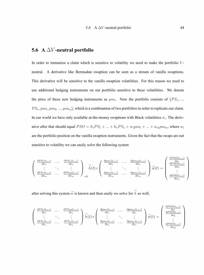
5.6 A �V -neutral portfolio 44
5.6 A�V -neutral portfolio
In order to immunize a claim which is sensitive to volatility we need to make the portfolio V -
neutral. A derivative like Bermudan swaption can be seen as a stream of vanilla swaptions.
This derivative will be sensitive to the vanilla swaption volatilities. For this reason we need to
use additional hedging instruments on our portfolio sensitive to these volatilities. We denote
the price of these new hedging instruments as psoi. Now the portfolio consists of fPS1; :::;
PSn; pso1; pso2; :::; psomg, which is a combination of two portfolios in order to replicate our claim.
In our world we have only available at-the-money swaptions with Black volatilities �i. The deriv-
ative after that should equal PSO = h1PS1 + ::: + hnPSn + w1pso1 + ::: + wmpsom, where wi
are the portfolio position on the vanilla swaption instruments. Given the fact that the swaps are not
sensitive to volatility we can easily solve the following system
0B@@PS1(ti+1)
@�1� � � @PSn(ti+1)
@�1... . . . ...@PS1(ti+1)
@�m� � � @PS10(ti+1)
@�m
1CA=0
!h(t)+
0B@@pso1(ti+1)
@�1� � � @pso10(ti+1)
@�1... . . . ...@pso1(ti+1)
@�m� � � @psom(ti+1)
@�m
1CA!w(t) =
0BBBB@@PSO(ti+1)
@�1@PSO(ti+1)
@�2...@PSO(ti+1)
@�m
1CCCCA
after solving this system !w is known and then easily we solve for
!h as well,
0B@@PS1(ti+1)
@r1� � � @PS10(ti+1)
@r1... . . . ...@PS1(ti+1)
@rn� � � @PSn(ti+1)
@rn
1CA!h(t)+
0B@@pso1(ti+1)
@r1� � � @psom(ti+1)
@r1... . . . ...@pso1(ti+1)
@rn� � � @psom(ti+1)
@rn
1CA!w(t) =
0BBBB@@PSO(ti+1)
@r1@PSO(ti+1)
@r2...@PSO(ti+1)
@r10
1CCCCA

5.6 A �V -neutral portfolio 45
5.6.1 A self-�nanced�V -hedging portfolio
As we de�ned above, we attempt to construct a replicating portfolio which is solely �nanced from
the wealth generated from its assets.
PSO(0) = V h(0) =
(nXi=1
hi(0)PSi(0)
)=0
+
(mXi=1
wi(0)psoi(0)
)6=0
+ hB(0)
On the next hedging step we liquidate the portfolio of swaps and swaptions. According to
pro�t or loss from the current positions we take a relevant cash position in order to go long on a
portfolio of new swaptions to make the total portfolio �V -neutral and with zero cost we buy a
portfolio of par swaps. Like that, the next rebalancing step is as follows
V h(1) =
(nXj=1
hj(1)PSj(1)
)=0
+
(mXj=1
wj(1)psoj(1)
)6=0
+ hB(1)
V h(2) =
(nXk=1
hk(2)PSk(2)
)=0
+
(mXk=1
wk(2)psok(2)
)6=0
+ hB(2)
...
where hB(t) is the cash adjustment, either long or short position on cash equivalent with the avail-
able cash from previous step and the additional cash generated from selling the previous swaps and
swaptions minus the cost of buying fw1(t); :::; wm(t)g swaptions. Like that, the value the portfolio
at time t worths
V h(t) =nXj=1
hj(t� 1)PSj(t) +mXj=1
wj(t� 1)psoj(t) + hB(t� 1)AF (t� 1; t)
then we liquidate and immediately at the same time we construct a new portfolio with new instru-
ments
V h(t) =
(nXk=1
hk(t)PSk(t)
)=0
+
mXk=1
wk(t)psok(t) + hB(t)

5.6 A �V -neutral portfolio 46
with cash position
hB(t) = Vh(t)�
(mXk=1
wk(t)psok(t)
)

Chapter 6Model risk and related errors
The principle of derivatives pricing indicates that the cost of replicating a new product should
equal its initial price. Hence, we are both interested to know how much our model values (initial
price and �nal hedging error) differ from the "real" ones, whenever model valuation is applied.
The quanti�cation of model risk in practice is more dif�cult than the methods presented in chapter
2. The reason is that model risk cannot be observed directly from the given prices.
To be able to study model risk extensively, �rst we need to identify the errors due to pricing,
hedging and market risk as separate14 random sources. With this chapter we attempt to identify
the sources of model risk as they might appear in practice. In this way we aim to help the readers
to create the �rst intuition about the problem and boost their understanding for the upcoming
results in chapters 7 and 8. The theory presented on the following sections will be the base of our
explanations for a wide variety of experimental results.
6.1 Errors on pricing
For the list below it holds that all random variables are de�ned on the same sample space (;F ;Q)
as we de�ned in chapter 2.
� Let F (t) a random variable which describes the �real� market price of product F at t.
14 For simplicity we assume independence between the random sources of risk. Any possible correlation structure (ifthere exists) between the random sources will require additional research which is not a part of the current project.
47

6.1 Errors on pricing 48
� Let F (t)M a random variable which describes the model price of product F at t, while no
parameter15 uncertainty is assumed.
� Let �(t)M = F (t)M � F (t) a random variable which describes the pricing error due to
modelM , while no parameter uncertainty is assumed.
� Let F (t)Mcalib a random variable which describes the model price of product F at t, while
the model is calibrated to liquid market instruments. At this stage we face parameter
uncertainty because of the estimation.
� Let �(t)Mcalib = F (t)Mcalib � FM(t) a random variable which describes the pricing error due
to calibration of modelM to liquid market instruments. This error depends on the quality
and liquidity of the market prices.
Proposition 3 The model price at t, when the model is marked-to-market, equals the �real�
market price plus the additional model errors,
F (t)Mcalib = �(t)Mcalib + �(t)
M + F (t) (6.22)
The total pricing error at t due to misspeci�ed modelM equals
�(t) = �(t)Mcalib + �(t)M (6.23)
15 Assume that we use the optimal model parameters according to the current market data.
6.2 Errors on hedging 49
6.2 Errors on hedging
The pricing error of equation (6.23) will play a role on the value of the hedging ratios. For a
discrete hedging portfolio this will cause an additional uncertainty on top of market risk16.
� Let V(t) a random variable which describes the price of the hedging portfolio at t while we
apply continuous rebalancing and the prices are driven by the true model.
� Let �(t)D a random variable which describes the price of hedging portfolio at t with
discrete rebalancing and the prices are driven by the true model.
� Let E(t)D = �(t)D � V(t) a random variable which describes the portfolio's error due
to discrete rebalancing. This error represents market risk. ED depends on the ability of
numerical hedging ratios to approximate suf�ciently the sensitivity of the claim to market
changes.
� Let �(t)MD a random variable which describes the price of the hedging portfolio at t with
discrete rebalancing, when model M is used for the approximation of the hedging ratios
and no parameter uncertainty is assumed for that model.
� Let E(t)MD = �(t)MD ��(t)D a random variable which describes the discrete portfolio error
due to misspeci�ed model M for discrete rebalancing while no parameter uncertainty is
assumed for that model.
16 Market risk is the risk due to the changes on market variables such as interest rates, swap rates, volatility, in�ation,etc.

6.3 Errors on a �-hedging portfolio 50
� Let �(t)MD;calib is a random variable which describes the model price of discretely rebalanced
portfolio at t when the misspeci�ed modelM is calibrated to liquid market instruments.
� Let E(t)MD;calib = �(t)MD;calib � �(t)MD a random variable which describes the discrete
portfolio error due to calibration of modelM to the current market data.
Proposition 4 The discrete model price of portfolio at time t while the model is marked-to-market
equals the price of the �real� portfolio plus the discretization error and model errors. Then the
price is
�(t)MD;calib = E(t)MD;calib + E(t)MD + E(t)D + V(t) (6.24)
The total hedging error for one discrete hedging step is
E(t) = E(t)MD;calib + E(t)MD + E(t)D (6.25)
and
E(t)M = E(t)MD;calib + E(t)MD (6.26)
is the additional error due to modelM when discrete rebalancing is applied.
6.3 Errors on a�-hedging portfolio
After keeping in mind proposition (1) and (2) we are able to apply the same logic on a �-hedging
portfolio. Suppose that we have a market which is consisted of the risky underlying S(t) given a
priori and de�ned on the probability space (;F ;Q). Then, the P-dynamics of the underlying are
given by
dS(t) = a(t)S(t)dt+ �(t)S(t)d_W (t) (6.27)

6.3 Errors on a �-hedging portfolio 51
Moreover, the market consists of a risk-free asset B(t) with dynamics
dB(t) = r(t)B(t)dt
_W (t) is a P-Wiener process and r(t) the instantaneous short rate.
Consider a derivative product F (t; S(t)) which produces T -claim X =F (T; S(T )) at T . As
it is shown in Bjork [2004] under the assumption of constant volatility the product F is tradable
only if it satis�es the following partial derivative (in terms of clarity we temporarily omit to show
the variables of the corresponding functions)
rF =@F
@t+ rS
@F
@S+1
2�2S2
@2F
@S2
with �nal condition X =F (T; S(T )). The above equation can be also seen as
rF = �+ rS�+1
2�2S2� (6.28)
In order to hedge this claim we need to construct a portfolio V(t) which must be able to
replicate the diffusion F (t; S(t)) , 8t 2 [0; T ]. Therefore, the diffusion V should have the same
sensitivity to market movements as F . Then a continuously rebalanced hedging portfolio V should
satisfy
rV = �+ rS�+ 12�2S2� (6.29)
After this step, assume that �(t) represents a �-hedging portfolio in continuous time. For
this portfolio � and � terms remain unhedged and the following equality holds
r� = rS� (6.30)

6.3 Errors on a �-hedging portfolio 52
while the portfolio error �E(t) for the �-hedging portfolio �(t) will be
�E = r�� rV
= ��� 12�2S2� (6.31)
Next, consider �(t) and �(t) in discrete time. We will denote them as �(t)D and �(t)D
respectively, such that the discretization error �ED due to �-hedging in discrete time is
�ED = r�D � r�
= rS(�D ��) (6.32)
Now suppose that we are in the inconvenient case that we have to use a model M for the
calculation of the hedging ratio �(t)D (no parameter uncertainty is assumed at this stage). We
denote the new portfolio as�(t)MD and the hedging ratio as�(t)MD . The use of model will introduce
an additional error in comparison with the previous portfolio �D which equals
�EMD = r�MD � r�D
= rS(�MD ��D) (6.33)
Furthermore, if modelM is calibrated to market data we denote�(t)MD;calib and �(t)MD;calib for the
calibrated �(t)MD and �(t)MD respectively. Then the calibration contributes to an extra error term
to the previous portfolio
�EMD;calib = r�MD;calib � r�MD
= rS(�MD;calib ��M
D ) (6.34)

6.4 Errors - Market risk - Model risk 53
Finally, the value of a discrete �-hedging portfolio is supported by a calibrated modelM is17
r�MD;calib = �EMD;calib + r�MD
= �EMD;calib +� EMD + r�D
= �EMD;calib +� EMD +� ED + r�
= �EMD;calib +� EMD +� ED +� E + rV (6.35)
After all this modi�cation the total hedging error which is included on the �nal price of portfolio
�MD;calib as a residual cost on excess of the �real� portfolio value V(t). Hence the total error equals
E = r�MD;calib � rV
= [�E ]Unhedged + f�EDgMarket +��EMD +� EMD;calib
�Model
(6.36)
6.4 Errors - Market risk - Model risk
E(t) is the random variable from which a P&L distribution is generated. The contribution of M
model to the total error E(t) for a discrete �-hedging strategy is
EM =� EMD +� EMD;calib (6.37)
� EM is the random term that will contribute to the diversity of the �nal hedging outcomes
along a set of different models.
� ED is the error term that remains unaffected from the use of any model. This term is
connected to the discreteness of the portfolio, the numerical approximation of the continuous
17 For the derivation of (6.35) we use equations (6.31), (6.32), (6.33), (6.34).

6.4 Errors - Market risk - Model risk 54
partial derivative � � @F@Sand the change of the market variable S through the life of
�nancial product F .
� �E which is composed from the remaining terms of the expansion (6.28) � and �. The �E
will not be affected from the set of candidate models. Moreover, �E may have additional
terms except from � and � if the Itô expansion (6.28) is applied on a different process
F (t; S(t)), e.g. F (t; �(t); S (t; �(t))).
�MD;calib will be the output of a usual hedge test. Therefore, E(t) can be derived by comparing
�MD;calib(t) to the price of the �nancial derivative F (t), where F moves with a different process than
�MD;calib. If a model-free F (t) is available, E(t) can be extracted at any time. Otherwise this is only
possible at time T where F (T ) = X .
After this description, we have a clear picture of the basic implementation and the risks that
we expect to affect the price of our results. The next two chapters are dedicated to present the
hedging outcomes based on the current infrastructure. On chapter 7 we present results from plain
vanilla interest rate claims. Using such products we validate (without the presence of benchmark
hedger) the accuracy of our results by identifying expected hedging errors. Any unexpected leak-
age on the portfolio would be considered as a bug. Taking advantage on the simplicity of these
payoffs, we perform some additional experiments to improve our understanding on the hedging
procedure and its related properties. For the experiments analytical (mark-to-market valuation)
and model-based (Monte-Carlo) pricing is applied. Finally, chapter 8 is focused on the most inter-
esting part of our research, which is the investigation of model risk on Callable swaps under the
valuation setting of chapter 4.

Chapter 7Results I: Hedge test
An important practical topic of model risk and risk management in general is the correct
implementation of a model. For that reason, the �rst part of this chapter is devoted to the validation
of our hedging module. The chapter is structured as follows.
The �rst section gives a brief introduction to the available market data. The second section
describes our validation strategy and the set of the experiments that are going to be applied. After
that the �, V and �V -hedging results of vanilla swaps and swaptions are presented.
The second part of this chapter is dedicated to provide additional explanations regarding the
performance and the user's choices of the replication. Topics that are discussed are the use of
forward and spot sensitivities, the hedging frequency and the bumping size of the hedging ratios.
Examples are also given as an evidence that the error decomposition is feasible when hedging
simulations are performed under several assumptions (see table (7.1)). All the explanations that
we currently provide are based on the error setting of chapter 6.
In all sections we apply mark-to-market (MtM) analytical pricing except from the last section
(7.5) where both MtM and Monte-Carlo pricing are being used.
7.1 Historical data
The set of historical scenarios is based on market data of swap rates and at-the-money (ATM)18
vanilla swaption volatilities. The graph below visualizes the quoted swap rates and few selected
18 No smile is available for the Black swaption volatilities.
55
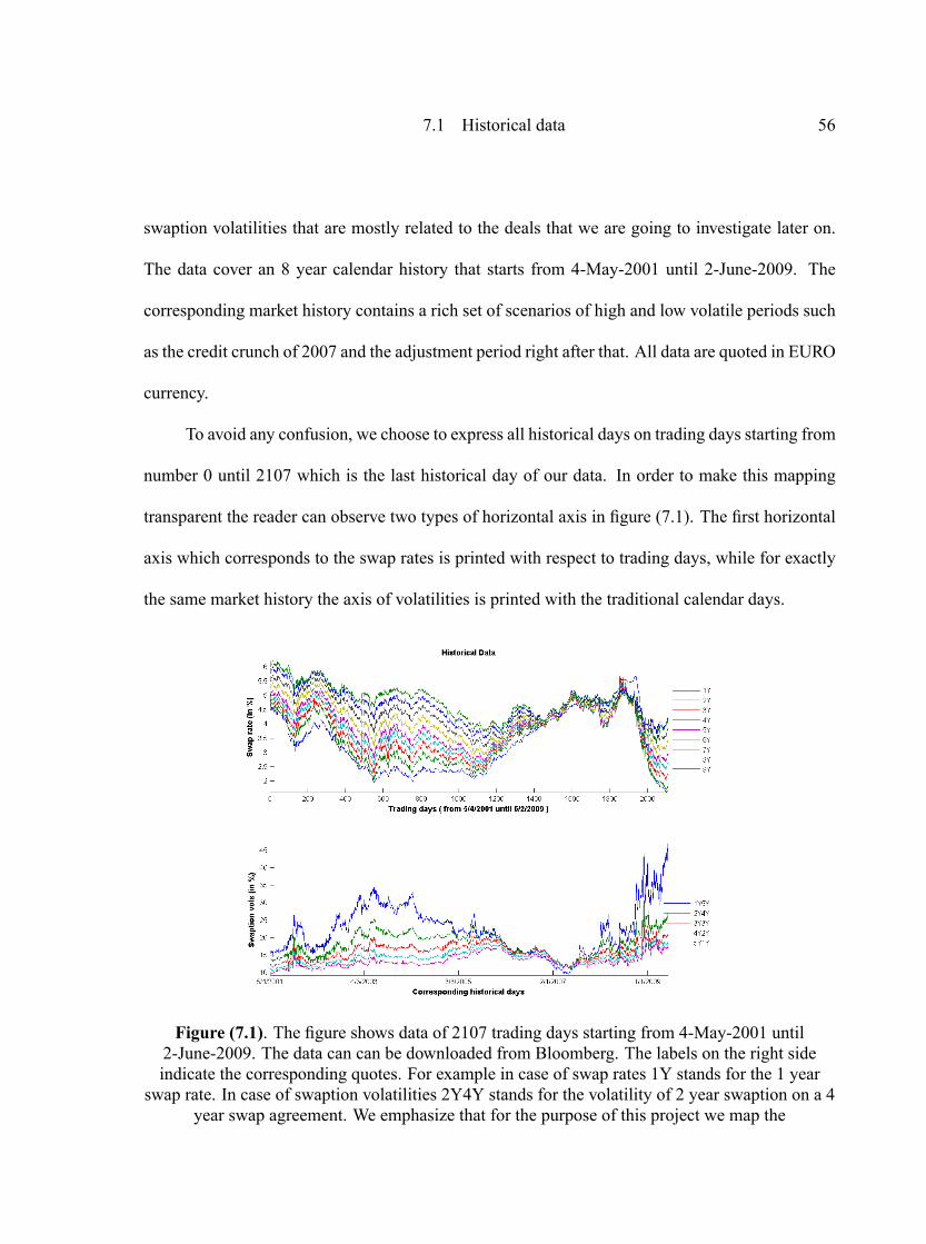
7.1 Historical data 56
swaption volatilities that are mostly related to the deals that we are going to investigate later on.
The data cover an 8 year calendar history that starts from 4-May-2001 until 2-June-2009. The
corresponding market history contains a rich set of scenarios of high and low volatile periods such
as the credit crunch of 2007 and the adjustment period right after that. All data are quoted in EURO
currency.
To avoid any confusion, we choose to express all historical days on trading days starting from
number 0 until 2107 which is the last historical day of our data. In order to make this mapping
transparent the reader can observe two types of horizontal axis in �gure (7.1). The �rst horizontal
axis which corresponds to the swap rates is printed with respect to trading days, while for exactly
the same market history the axis of volatilities is printed with the traditional calendar days.
Figure (7.1). The �gure shows data of 2107 trading days starting from 4-May-2001 until2-June-2009. The data can can be downloaded from Bloomberg. The labels on the right sideindicate the corresponding quotes. For example in case of swap rates 1Y stands for the 1 year
swap rate. In case of swaption volatilities 2Y4Y stands for the volatility of 2 year swaption on a 4year swap agreement. We emphasize that for the purpose of this project we map the

7.2 Validation strategy 57
corresponding calendar days to an equivalent trading day starting from 0 to 2107 which is thetotal number of the available history. All values are printed on percentage scale.
7.2 Validation strategy
For the validation of our hedging module we apply hedging on spot and forward starting vanilla
swaps and vanilla swaptions. These are the closest interest rate products to our hedging instru-
ments.
Experiment Hedging Type Time Rates Vols Unhedged RisksD1 �-hedging - change - �D2 �-hedging change change - � + �D3 �-hedging change change change � + �+ V + VD4 �-hedging - change change � + V + VV1 V -hedging - - change VV2 V -hedging change - change �+ VV3 V -hedging change change change �+ �+�+ VV4 V -hedging - change change �+ �+ VDV1 �V -hedging - change change � + VDV2 �V -hedging change change change � + �+ V
Table 7.1. The table lists all the experiment types of the validation strategy. Each experimentimplements different type of hedging under several assumptions. The marker �-� means that thefactor speci�ed in the column label does not change during hedging process, while the marker�change� stands for the opposite. The last column on the right hand side shows the risk factorswhich remain unhedged according to the type of hedging which is indicated on the second column.V stands for Volga.
To test extensively the performance of our module we perform hedging under different as-
sumptions. The validation will be based on testing the performance of the hedger module in pres-
ence of different combinations of risk factors, like �, �, � and V . According to this idea we
need to de�ne a set of experiments that control the change of time (evaluation date), swap rates
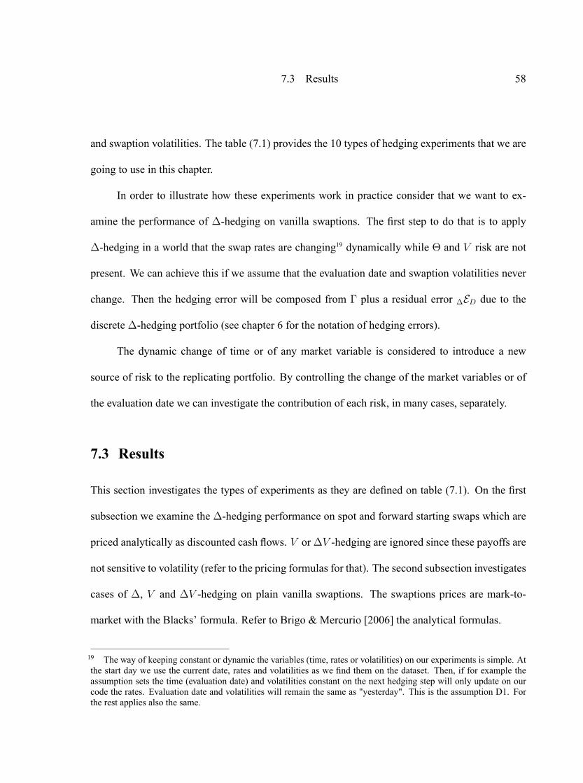
7.3 Results 58
and swaption volatilities. The table (7.1) provides the 10 types of hedging experiments that we are
going to use in this chapter.
In order to illustrate how these experiments work in practice consider that we want to ex-
amine the performance of �-hedging on vanilla swaptions. The �rst step to do that is to apply
�-hedging in a world that the swap rates are changing19 dynamically while � and V risk are not
present. We can achieve this if we assume that the evaluation date and swaption volatilities never
change. Then the hedging error will be composed from � plus a residual error �ED due to the
discrete �-hedging portfolio (see chapter 6 for the notation of hedging errors).
The dynamic change of time or of any market variable is considered to introduce a new
source of risk to the replicating portfolio. By controlling the change of the market variables or of
the evaluation date we can investigate the contribution of each risk, in many cases, separately.
7.3 Results
This section investigates the types of experiments as they are de�ned on table (7.1). On the �rst
subsection we examine the �-hedging performance on spot and forward starting swaps which are
priced analytically as discounted cash �ows. V or�V -hedging are ignored since these payoffs are
not sensitive to volatility (refer to the pricing formulas for that). The second subsection investigates
cases of �, V and �V -hedging on plain vanilla swaptions. The swaptions prices are mark-to-
market with the Blacks' formula. Refer to Brigo & Mercurio [2006] the analytical formulas.
19 The way of keeping constant or dynamic the variables (time, rates or volatilities) on our experiments is simple. Atthe start day we use the current date, rates and volatilities as we �nd them on the dataset. Then, if for example theassumption sets the time (evaluation date) and volatilities constant on the next hedging step will only update on ourcode the rates. Evaluation date and volatilities will remain the same as "yesterday". This is the assumption D1. Forthe rest applies also the same.

7.3 Results 59
We choose to perform hedging for almost 3 months period (61 trading days). This amount
of hedging steps is enough to give us the evidence we need in order to illustrate the consistent
behavior of the hedging module and verify the error description of chapter 6. On the results we
associate positive errors to pro�t and negative errors to loss. In this section we apply hedging based
on mark-to-market analytical formulas, hence there is no presence of model risk.
7.3.1 Vanilla swaps
Below we present D1 (only swap rates change) and D2 (swap rate and time change) type of �-
hedging experiments. On ATM spot starting swap of 3 years and ATM 1 year forward starting
swap of the same maturity are tested.
The �rst indication that the replication is working correctly is to use the fact that these instru-
ments can be perfectly replicated on the start day of the deal by the equivalent hedging instruments.
A short position on a 3 year swap can be replicated from a long 3 years swap hedging instrument.
A short position on a 1Y3Y swap can be replicated with a long 4 years swap and a short 1 year
swap.
The �gures below include the Net Present Values (NPV) of the option and that of the repli-
cating portfolio. The replication evolves along the axis of trading days. For hedging we use
double-sided forward sensitivities with bumping size of 8bps (see section (7.4.2) and section (7.4.4)
respectively).
The �rst hedge test shows almost perfect replication for the D1 case. Swaps are linear payoffs
and theoretically there is no convexity. This can be observed on the D1 error which is zero apart
from one day out of sixty days. The mismatch in this example might be either a discreteness or
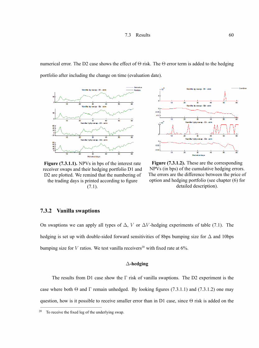
7.3 Results 60
numerical error. The D2 case shows the effect of � risk. The � error term is added to the hedging
portfolio after including the change on time (evaluation date).
Figure (7.3.1.1). NPVs in bps of the interest ratereceiver swaps and their hedging portfolio D1 andD2 are plotted. We remind that the numbering ofthe trading days is printed according to �gure
(7.1).
Figure (7.3.1.2). These are the correspondingNPVs (in bps) of the cumulative hedging errors.The errors are the difference between the price ofoption and hedging portfolio (see chapter (6) for
detailed description).
7.3.2 Vanilla swaptions
On swaptions we can apply all types of �, V or �V -hedging experiments of table (7.1). The
hedging is set up with double-sided forward sensitivities of 8bps bumping size for � and 10bps
bumping size for V ratios. We test vanilla receivers20 with �xed rate at 6%.
�-hedging
The results from D1 case show the � risk of vanilla swaptions. The D2 experiment is the
case where both � and � remain unhedged. By looking �gures (7.3.1.1) and (7.3.1.2) one may
question, how is it possible to receive smaller error than in D1 case, since � risk is added on the
20 To receive the �xed leg of the underlying swap.

7.3 Results 61
portfolio? This example gives a good motivation that further analysis is required if we want to
understand and �nally measure the errors of our replicating strategy.
Figure (7.3.2.1). NPVs in bps of vanilla receiverswaptions and their hedging portfolio D1, D2, D3and D4 are plotted. We remind that the numberingof the trading days is printed according to �gure
(7.1).
Figure (7.3.2.2). These are the correspondingNPVs (in bps) of the cumulative hedging errors.The errors are the difference between the price ofoption and hedging portfolio (see chapter (6) for
detailed description).
The experiments emphasize that receiving small errors does not imply low risk or good
hedging performance. As we will see on the next section (7.4.1) � and � risks partially cancel out
with each other. Hence, we cannot relate the size of hedging error directly to performance without
any further analysis. As a consequence, the impact of �hidden� risk factors will remain the main
obstacle for the model risk quanti�cation.
D3 is the type of �-hedging where time, swap rates and swaption volatilities are changing
during the life of the experiment. In this case we see that the impact of volatility risk ampli�es the
hedging error in comparison with the D2 case. The error of experiment D3 as it is stated on table
(2) leaves unhedged �, �, V and V. D4 experiment is the last of the �-hedge tests, in that case
time is ignored. � risk is not anymore on the portfolio and this moves the hedging error to more

7.3 Results 62
loss. This is the second evidence together with the D2 errors which show that � risk has a positive
sign for this portfolio.
V -hedging
The results for a vega hedged portfolio are also interesting. The �rst observation is that V is
relatively smaller than the realized � errors (see D1 case on �gure (7.3.2.2) for the size of �). This
is not an occasional observation. We verify that the performance of a V -hedging portfolio is not
signi�cantly affected by using different bumping sizes for hedging. For a range [0.1-200]bps of
several bumping sizes we tested the hedging performance with no important differences. The vari-
ability of the results was approximately a couple of basis points. The V2 hedging error shows the
contribution� risk to the vega hedged portfolio. The V3 type of hedging, in addition, incorporates
the unhedged � and � terms to the portfolio and V4 includes all risks except from �.
Figure (7.3.2.3). NPVs in bps of vanilla receiverswaptions and their hedging portfolio V1, V2, V3and V4 are plotted. We remind that the numberingof the trading days is printed according to �gure
(7.1).
Figure (7.3.2.4). These are the correspondingNPVs (in bps) of the cumulative hedging errors.The errors are the difference between the price ofoption and hedging portfolio (see chapter (6) for
detailed description).
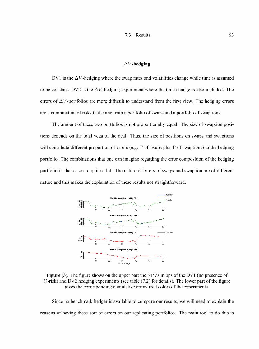
7.3 Results 63
�V -hedging
DV1 is the �V -hedging where the swap rates and volatilities change while time is assumed
to be constant. DV2 is the �V -hedging experiment where the time change is also included. The
errors of �V -portfolios are more dif�cult to understand from the �rst view. The hedging errors
are a combination of risks that come from a portfolio of swaps and a portfolio of swaptions.
The amount of these two portfolios is not proportionally equal. The size of swaption posi-
tions depends on the total vega of the deal. Thus, the size of positions on swaps and swaptions
will contribute different proportion of errors (e.g. � of swaps plus � of swaptions) to the hedging
portfolio. The combinations that one can imagine regarding the error composition of the hedging
portfolio in that case are quite a lot. The nature of errors of swaps and swaption are of different
nature and this makes the explanation of these results not straightforward.
Figure (3). The �gure shows on the upper part the NPVs in bps of the DV1 (no presence of�-risk) and DV2 hedging experiments (see table (7.2) for details). The lower part of the �gure
gives the corresponding cumulative errors (red color) of the experiments.
Since no benchmark hedger is available to compare our results, we will need to explain the
reasons of having these sort of errors on our replicating portfolios. The main tool to do this is
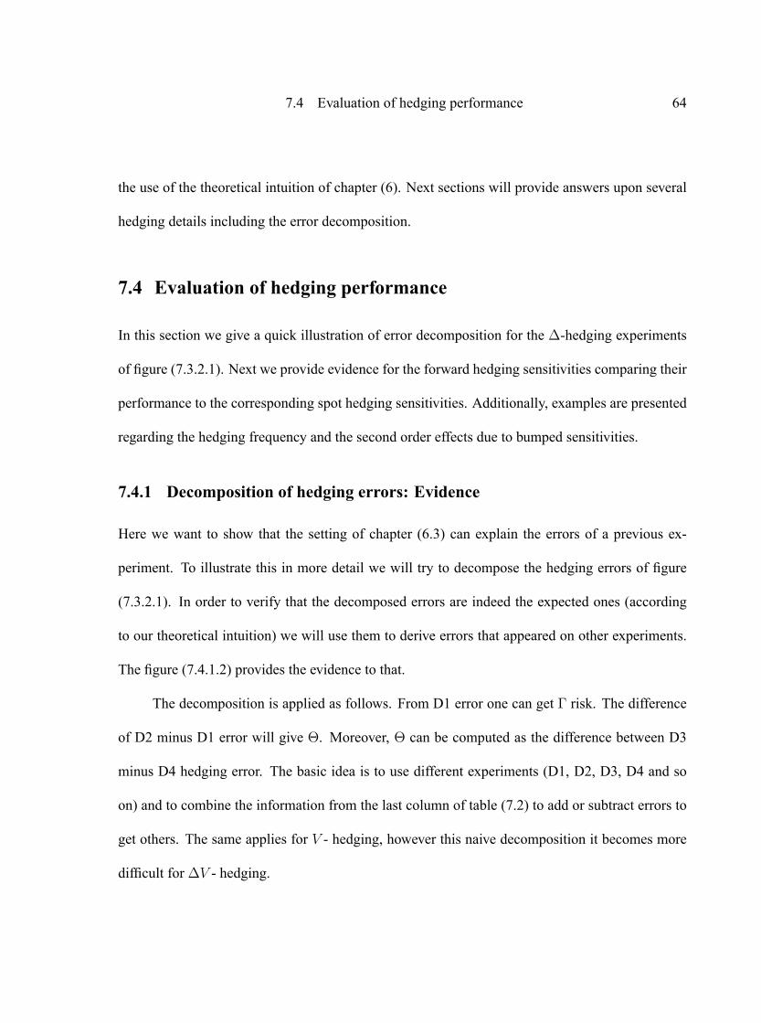
7.4 Evaluation of hedging performance 64
the use of the theoretical intuition of chapter (6). Next sections will provide answers upon several
hedging details including the error decomposition.
7.4 Evaluation of hedging performance
In this section we give a quick illustration of error decomposition for the �-hedging experiments
of �gure (7.3.2.1). Next we provide evidence for the forward hedging sensitivities comparing their
performance to the corresponding spot hedging sensitivities. Additionally, examples are presented
regarding the hedging frequency and the second order effects due to bumped sensitivities.
7.4.1 Decomposition of hedging errors: Evidence
Here we want to show that the setting of chapter (6.3) can explain the errors of a previous ex-
periment. To illustrate this in more detail we will try to decompose the hedging errors of �gure
(7.3.2.1). In order to verify that the decomposed errors are indeed the expected ones (according
to our theoretical intuition) we will use them to derive errors that appeared on other experiments.
The �gure (7.4.1.2) provides the evidence to that.
The decomposition is applied as follows. From D1 error one can get � risk. The difference
of D2 minus D1 error will give �. Moreover, � can be computed as the difference between D3
minus D4 hedging error. The basic idea is to use different experiments (D1, D2, D3, D4 and so
on) and to combine the information from the last column of table (7.2) to add or subtract errors to
get others. The same applies for V - hedging, however this naive decomposition it becomes more
dif�cult for �V - hedging.

7.4 Evaluation of hedging performance 65
Figure (7.4.1.1). NPVs in bps of the vanilla swap-tions and their hedging portfolio are plotted. Thisis the same as �gure(7.3.2.5). It is given next tothe decomposed examples to assist the visual
inspection.
Figure (7.4.1.2).These are the correspondingNPVs of the cumulative hedging errors. The er-rors are analysed and reproduced by using the
assumptions of table (7.2).
The promising message of this example is that by using a set independent experiments (hedge
tests) we are able to reproduce errors or remove artifacts from our data. This fact will be used later
on chapter (9) to recommend a possible solution for more complicated problems.
7.4.2 Forward vs Spot sensitivities: Robustness
On the following �gures we will provide two examples as an evidence on the choice of using
forward instead of spot sensitivities on our hedging. The �rst example considers a 3 and 10 years
ATM vanilla swap that receives �xed. The second example examines the effect of forward and spot
sensitivities on a non-linear deal. For this reason a vanilla swaption is replicated. Both examples
are D2 type of hedging experiment, where �- hedging is applied while time (evaluation date) and
swap rates are changing dynamically.
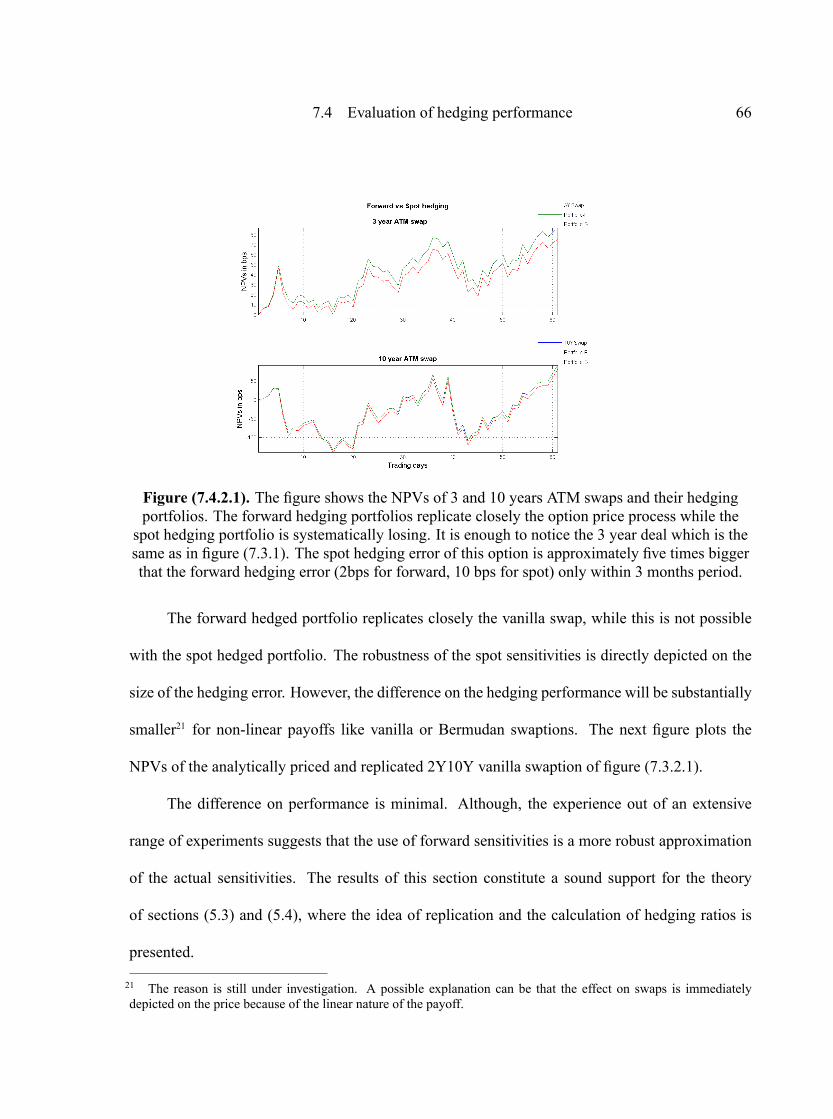
7.4 Evaluation of hedging performance 66
Figure (7.4.2.1). The �gure shows the NPVs of 3 and 10 years ATM swaps and their hedgingportfolios. The forward hedging portfolios replicate closely the option price process while thespot hedging portfolio is systematically losing. It is enough to notice the 3 year deal which is thesame as in �gure (7.3.1). The spot hedging error of this option is approximately �ve times biggerthat the forward hedging error (2bps for forward, 10 bps for spot) only within 3 months period.
The forward hedged portfolio replicates closely the vanilla swap, while this is not possible
with the spot hedged portfolio. The robustness of the spot sensitivities is directly depicted on the
size of the hedging error. However, the difference on the hedging performance will be substantially
smaller21 for non-linear payoffs like vanilla or Bermudan swaptions. The next �gure plots the
NPVs of the analytically priced and replicated 2Y10Y vanilla swaption of �gure (7.3.2.1).
The difference on performance is minimal. Although, the experience out of an extensive
range of experiments suggests that the use of forward sensitivities is a more robust approximation
of the actual sensitivities. The results of this section constitute a sound support for the theory
of sections (5.3) and (5.4), where the idea of replication and the calculation of hedging ratios is
presented.
21 The reason is still under investigation. A possible explanation can be that the effect on swaps is immediatelydepicted on the price because of the linear nature of the payoff.
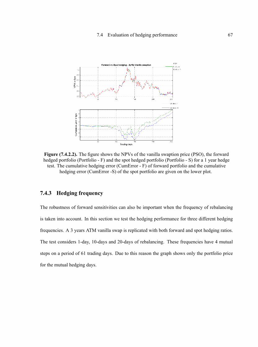
7.4 Evaluation of hedging performance 67
Figure (7.4.2.2). The �gure shows the NPVs of the vanilla swaption price (PSO), the forwardhedged portfolio (Portfolio - F) and the spot hedged portfolio (Portfolio - S) for a 1 year hedgetest. The cumulative hedging error (CumError - F) of forward portfolio and the cumulative
hedging error (CumError -S) of the spot portfolio are given on the lower plot.
7.4.3 Hedging frequency
The robustness of forward sensitivities can also be important when the frequency of rebalancing
is taken into account. In this section we test the hedging performance for three different hedging
frequencies. A 3 years ATM vanilla swap is replicated with both forward and spot hedging ratios.
The test considers 1-day, 10-days and 20-days of rebalancing. These frequencies have 4 mutual
steps on a period of 61 trading days. Due to this reason the graph shows only the portfolio price
for the mutual hedging days.

7.4 Evaluation of hedging performance 68
Figure (7.4.3). The �gure shows spot (S) and forward (F) hedged portfolios. The D2 type of�-hedging is performed for 1, 10 and 20 days of rebalancing frequency. We plot NPVs of thederivative and its corresponding portfolios for only the 4 common steps of the different hedgingfrequencies. The hedging is applied on a 3 year ATM swap. PSO stands for the derivatives' price.
The forward sensitivities seem to be more robust for any of the hedge tests. The effect of
spot sensitivities is quite more important on linear products and this is the reason that we have used
swaps for our example.
In order not to create any confusion, we emphasize that the forward sensitivities do not hedge
� (see the presence of�-risk on previous �gures). The forward hedging portfolios on �gure (7.4.3)
are very close to the price of the vanilla swap (see the bold blue dashed line in the previous �gure)
while the errors are too small to be visible (see �gure (7.3.1) for the magnitude of the hedging
errors on swaps)
It is good to mention that the hedging frequency is not correlated with the hedging perfor-
mance as we see on the �gure above. This is because the hedging ratio will approximate the real
sensitivity in presence of market risk. On the next rebalancing step the hedge will perform accord-
ing to the movement of the market. The size of the market movement is not always dependent to
the observation time (herein hedging frequency). Hence, the error of rebalancing in discrete time

7.4 Evaluation of hedging performance 69
will not be directly connected to the size of the hedging frequency. Spot sensitivities show that are
more vulnerable to market risk and hedging frequency than the forward sensitivities. This is the
�nal evidence that we needed to support the consistency of equation (5.19).
7.4.4 Bumping size: The effect of second-order risks
One of the last things that we need to investigate, before we start the model risk experiments, is
the choice of bumping sizes for the hedging ratios. As we have mentioned at the beginning of
this chapter we used two sided bumped sensitivities. For the calculation of � ratios we use 8bps
bumping size and for V ratios 10bps. The reason of choosing these bumping sizes is due to the fact
that the standard deviation of the the daily changes of the quoted rates is around 5-6bps on a yearly
periods. The standard deviation of the daily changes for swaption volatilities is around 10-15bps
on a yearly bootstrapping window. The effect of second order risks of V is very small as we have
already mentioned in section (7.3.2). On the other hand the effect of � risk is more important and
the choice of the bumping size for � is crucial.
Piterbarg [2005], for a similar replication problem on Bermudan swaptions, remarks that a
reasonable bumping size may be 10bps for �. Of course, this remark is based on different market
data. Making several hedging experiments on our data we observed that 8bps is a fairly good
choice. This bumping size is a bit higher22 than the standard deviation of the daily increments of
quoted swap rates.
22 Piterbarg also mentions that a bigger bumping size may hedge a part of second order terms.

7.4 Evaluation of hedging performance 70
In the �gure below we show the effect of � risk on the portfolio of the previous 2Y10Y
vanilla swaption under the assumptions of D1 experiment where no � is taken into account. Then
the observed errors associate to � risk only.
Figure (7.4.4). The �gure shows the NPVs of the hedging errors of a D1 type of experiment on a2y10y vanilla swaption. The errors in that case show only the �-risk.
The �gure shows that different bumping sizes may perform better from one scenario to an-
other. As an example we give �gure (7.4.4). The bumped sensitivities of 125 and 175 bps result
lower errors on the tested period. Although, on average bumping sizes higher that 15bps will give
higher errors in a wide range of market scenarios. The choice of bumping size does not have a
�xed rule and always depends on the market scenarios.
The size of 8 and 10 bps for � and V respectively, based on the standard deviation of the
data increments, proves to be a good choice for the current dataset. The errors that we receive with
these estimates do not exceed the absolute value of 45bps even on a 5 year horizon.
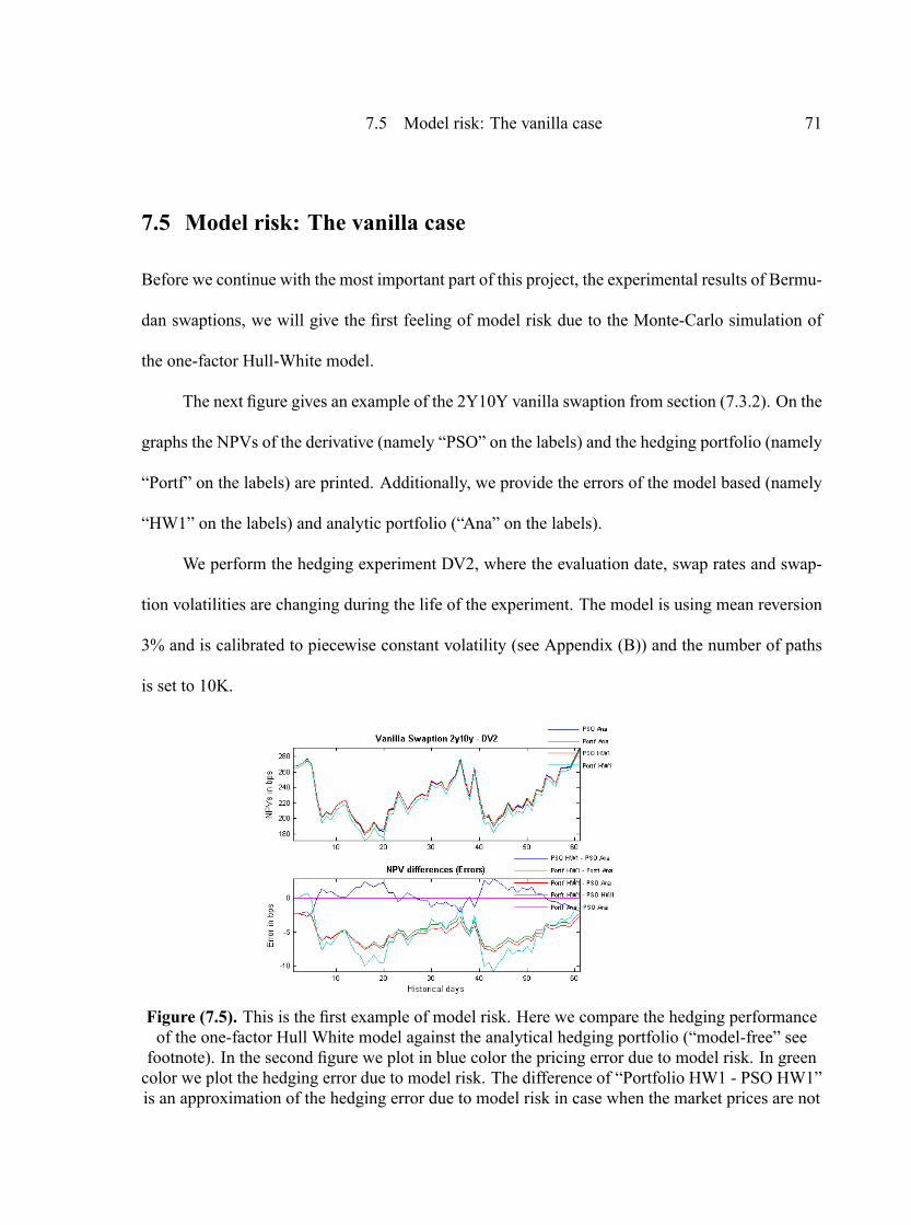
7.5 Model risk: The vanilla case 71
7.5 Model risk: The vanilla case
Before we continue with the most important part of this project, the experimental results of Bermu-
dan swaptions, we will give the �rst feeling of model risk due to the Monte-Carlo simulation of
the one-factor Hull-White model.
The next �gure gives an example of the 2Y10Y vanilla swaption from section (7.3.2). On the
graphs the NPVs of the derivative (namely �PSO� on the labels) and the hedging portfolio (namely
�Portf� on the labels) are printed. Additionally, we provide the errors of the model based (namely
�HW1� on the labels) and analytic portfolio (�Ana� on the labels).
We perform the hedging experiment DV2, where the evaluation date, swap rates and swap-
tion volatilities are changing during the life of the experiment. The model is using mean reversion
3% and is calibrated to piecewise constant volatility (see Appendix (B)) and the number of paths
is set to 10K.
Figure (7.5). This is the �rst example of model risk. Here we compare the hedging performanceof the one-factor Hull White model against the analytical hedging portfolio (�model-free� seefootnote). In the second �gure we plot in blue color the pricing error due to model risk. In greencolor we plot the hedging error due to model risk. The difference of �Portfolio HW1 - PSO HW1�is an approximation of the hedging error due to model risk in case when the market prices are not

7.5 Model risk: The vanilla case 72
available.
Difference in bps Relative errorPricing Model Error -1.935 -0.663%Portfolio HW1 - PSO Ana -2.616 -0.896%Portfolio HW1 - Portfolio Ana -2.102 -0.720%Portfolio HW1 - PSO Ana - Pricing Model Error -0.681 -0.233%Portfolio HW1 - PSO HW1 -0.681 -0.233%Portfolio Ana - PSO Ana 0.004 0.001%
Table 7.2. This table shows the �nal error differences of the Monte-Carlo and analytical prices of�gure (7.5). The relative errors are elements of the �rst column over the last MtM swaption price.
In case of liquid products the actual difference between the model and �model-free� 23 cumu-
lative errors can be interpreted as the model risk of the hedging portfolio. The extraction of model
risk for non liquid products will not be that easy. The study of model risk for exotic products does
not have available the �model-free� derivative prices. The analysis of exotic portfolios requires a
very good understanding of market and model risk impact on the �nal prices. This was exactly the
scope of this chapter, to warm up the reader's understanding of the �nal experiments that follow
in chapter 8. For the next of the experiments the difference �Portfolio HW1 - PSO Ana - Pricing
Model Error� will be the approximation of the hedging error due to model risk.
23 �Model-free portfolio�: The mark-to-market prices of vanilla swaptions are quoted as volatilities that are used asinput to Black's formula to get the market price. Hence the hedged portfolio which uses this analytical formula isconsidered to be model free.

Chapter 8Results II: Model risk assessment
For the model risk assessment there are two options of testing the parameter and model uncer-
tainty. In order to study the performance of different models it is required that models should have
suf�ciently speci�ed their structural parameters to be consistent with the market prices (internally
consistent model). The wrong use of internal parameters can push a model to substantial losses
(take as an example the results of Longstaff, Santa-Clara & Schwartz [2001] ref.[22]). Hence, be-
fore the experimenter proceeds to the study of model uncertainty it is important to start from the
internal consistency of his/her models. As a consequence on this project we will restrict on the
mean reversion uncertainty of the one-factor Hull-White model on Bermudan swaptions.
The uncertainty on our model remains on the mean reversion parameter � since � is cal-
ibrated as a piecewise constant parameter. The mean reversion parameter is responsible for the
shape (curvature) of the volatility structure (see section (4.1.2)). The speci�cation of this parame-
ter for Bermudan swaptions is recommended for the range or [0-5]% for short and [0-3]% for long
maturity deals (see validation report [66]). On our experiments the range of the �nal hedging error
translates to a range of 15bps for short and 70bps for long maturity deals. The ranges of � are set
to {-1,1,3,10}% and {-1,1,3,5}% respectively for a notional of 10000bps in EURO.
For the experimental part of this chapter we start with the introduction of our methodology
including de�nition of experiments, collection of observations, data preprocessing and data analy-
sis. We separate our experiments with respect to riskiness and we present the results according to
that.
73

8.1 Methodology 74
The analysis of our experimental observations includes methods to imply correlation struc-
tures within the data and the formation of distinct clusters due to the effect of mean reversion factor.
The results of 5 and 20 years deals are presented separately and for their description an extensive
variety of graphical tools is being used.
At the end of the chapter we are speculating upon the results and a possible practical way to
estimate model risk and the mean reversion uncertainty. To illustrate this we give a short example
applied to our data and we leave the suggestions of its use for further investigation.
8.1 Methodology
The �rst task of our research is to produce a signi�cant amount of results that will cover a fairly
wide range of scenarios. The market scenarios24 we use are described in �gure (7.1). The trivial
idea to hedge the options up to maturity, in order to use the model free payoff price at expiry,
cannot be applied at this stage. This would require a huge amount of market scenarios which is
practically not feasible. The available market data cover a period of 8 trading years. One hedge
test may be enough to use the whole period of our data. Then the next experiment will be highly
correlated to the previous one.
Another issue which is related to callable options is that the contracts can be �nalized be-
fore their maturity. Then we face the following problem. For instance, imagine that a 10 year
Bermudan swaption annually exercised is called after 4 years under a certain scenario. For another
scenario the same product is exercised in two years. Under this situation we cannot analyze the
24 The real market scenarios are considered as �model-free� compared to arti�cially generated scenarios. Nonethe-less, market scenarios are associated with the past, while models are supposed to forecast the future. Hence, the marketscenarios of previous market history still suffer from identi�cation risk.
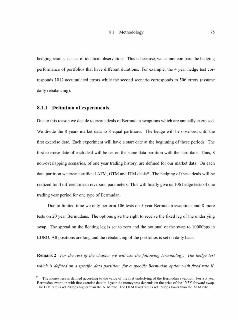
8.1 Methodology 75
hedging results as a set of identical observations. This is because, we cannot compare the hedging
performance of portfolios that have different durations. For example, the 4 year hedge test cor-
responds 1012 accumulated errors while the second scenario corresponds to 506 errors (assume
daily rebalancing).
8.1.1 De�nition of experiments
Due to this reason we decide to create deals of Bermudan swaptions which are annually exercised.
We divide the 8 years market data to 8 equal partitions. The hedge will be observed until the
�rst exercise date. Each experiment will have a start date at the beginning of these periods. The
�rst exercise date of each deal will be set on the same data partition with the start date. Thus, 8
non-overlapping scenarios, of one year trading history, are de�ned for our market data. On each
data partition we create arti�cial ATM, OTM and ITM deals25. The hedging of these deals will be
realized for 4 different mean reversion parameters. This will �nally give us 106 hedge tests of one
trading year period for one type of Bermudan.
Due to limited time we only perform 106 tests on 5 year Bermudan swaptions and 8 more
tests on 20 year Bermudans. The options give the right to receive the �xed leg of the underlying
swap. The spread on the �oating leg is set to zero and the notional of the swap to 10000bps in
EURO. All positions are long and the rebalancing of the portfolios is set on daily basis.
Remark 2 For the rest of the chapter we will use the following terminology. The hedge test
which is de�ned on a speci�c data partition, for a speci�c Bermudan option with �xed rate K,
25 The moneyness is de�ned according to the value of the �rst underlying of the Bermudan swaption. For a 5 yearBermudan swaption with �rst exercise date in 1 year the moneyness depends on the price of the 1Y5Y forward swap.The ITM rate is set 200bps higher than the ATM rate. The OTM �xed rate is set 150bps lower than the ATM rate.
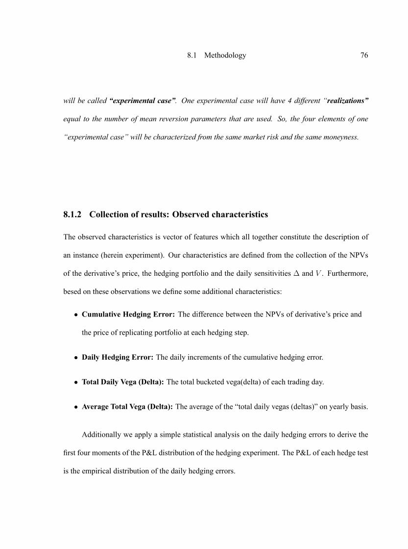
8.1 Methodology 76
will be called �experimental case�. One experimental case will have 4 different �realizations�
equal to the number of mean reversion parameters that are used. So, the four elements of one
�experimental case� will be characterized from the same market risk and the same moneyness.
8.1.2 Collection of results: Observed characteristics
The observed characteristics is vector of features which all together constitute the description of
an instance (herein experiment). Our characteristics are de�ned from the collection of the NPVs
of the derivative's price, the hedging portfolio and the daily sensitivities � and V . Furthermore,
besed on these observations we de�ne some additional characteristics:
� Cumulative Hedging Error: The difference between the NPVs of derivative's price and
the price of replicating portfolio at each hedging step.
� Daily Hedging Error: The daily increments of the cumulative hedging error.
� Total Daily Vega (Delta): The total bucketed vega(delta) of each trading day.
� Average Total Vega (Delta): The average of the �total daily vegas (deltas)� on yearly basis.
Additionally we apply a simple statistical analysis on the daily hedging errors to derive the
�rst four moments of the P&L distribution of the hedging experiment. The P&L of each hedge test
is the empirical distribution of the daily hedging errors.

8.1 Methodology 77
8.1.3 Data analysis
The scope of the data analysis is to identify which of the observed characteristics are systematically
being affected from the mean reversion uncertainty.
The initial inspection of the hedge test results combines visualization of the NPVs including
the portfolio's price, the hedging errors and the bucketed sensitivities. Additionally we provide the
P&L histogram and the quantile-quantile26 plot (Q-Q plot) of the daily hedging errors. This part
of the analysis is to make us familiar with the observed data (results) and if possible to identify a
sound behavior due to the different speci�cations of each experiment.
For the analysis of the collected data, with respect to mean reversion, we normalize the ob-
served characteristics of each experiment. The characteristic values of each individual experiment
then are transformed to standard normal variables on the following table.
MeanReversion Final error 1 Normalized Final error 11% 1.1 -0.24019-1% 1.4 1.2009613% 0.9 -1.200965% 1.2 0.240192
Group Mean 1.15 0Group St.Deviation 0.208167 1
Table 8.3. The table illustrates an example of data normalization. Consider an arbitrary experi-mental case of 4 mean reversions {1%, -1%, 3%, 5%}. From these mean reversions we get a groupof 4 different errors x. The mean � and standard deviation � of the group is calculated and the val-ues x are normalized as z = x��
�. On this table the values of the second column are the original
observations. The normalized characteristics are given on the third column. The normalized val-ues represent the effect of mean reversion on each characteristic value. The same applies to othercharacteristics.
26 Quantile-Quantile plot is a graphical method for comparing two probability distributions by plotting their quantilesagainst each other. Usually, the comparison is between the empirical and a theoretical distribution.

8.2 Hedge test results: 5 year Bermudan swaption 78
The normalization is a necessary step once we cannot compare values of different data pe-
riods and of different moneyness on the same axis. This procedure is a naive way to eliminate
market risk effects from our data.
After this step classi�cation analysis is performed using scatter27 and silhouette28 diagrams.
This procedure is a standard practice of data classi�cation (see Duda, Hart & Stork [2001]). This
analysis will show which characteristic values does the mean reversion parameter affect.
At the end of our analysis we apply a rough estimate of model risk for our deals. The estimate
will be a combination of the deviation and the riskiness of each experimental case.
8.2 Hedge test results: 5 year Bermudan swaption
We perform 106 hedge tests according to section (8.1.1). The replicating portfolio is based on
forward hedging ratios. For these hedge tests we de�ne an �experimental case� for {-1,1,3,10}%
mean reversions. -1% and 10% are extreme values while 1% and 3% are within the practice stan-
dards (see validation report [66]). The model is calibrated to 5 vanilla swaptions with maturities
that cover all the exercise dates of the Bermudan swaption. Hence we will have in total 5 bucketed
vegas. The number of Monte-Carlo paths is set to 25K.
27 A scatter plot is used when the observation parameter is under the control of the experimenter. The scope ofscatter plot is to show if a parameter is systematically increased or decreased by another one. The parameter whichis responsible for change of other parameters it is called the control parameter and is traditionally plotted along thehorizontal axis. Scatter plots can suggest various kinds of correlations between variables with a certain con�denceinterval.28 Silhouettes use the internal point distance to assign values from -1 to 1 to cluster points (see appendix (C). Themeasure shows of how similar that point is to points in its own cluster in comparison with points in other clusters.Values close to -1 implies that the point should belong to another cluster, 1 implies prefect �t with its cluster and 0 thatthe point cannot be an element of any cluster according to its internal point distance.

8.2 Hedge test results: 5 year Bermudan swaption 79
The visual inspection of the hedge tests have shown that the market scenarios and the mon-
eyness of the experiment affect signi�cantly the performance of hedging and the P&L of the daily
hedging errors. Meanwhile, the mean reversion does not contribute to big changes on the �nal
values. The results at the �rst stage suggest three main types of hedging behaviors.
The �rst type of hedging behavior is observed when vega is high. In that case, the hedging
error is very sensitive to market movements. The associated deals are non ITM during the life of
the experiment. These types of experiments will show signi�cant second order effects. Due to high
vega the hedging portfolio, in that cases, will be mainly consisted of vanilla swaption instruments.
The second category of hedging outcomes is when vega is small then the effect of market
risk is minimal. The Bermudan is ITM and converges to the underlying forward swap. Thus, the
product is transformed to a linear product. The option is almost not sensitive to volatility anymore.
The second order effects are dramatically reduced and the most important type of risk that affects
the portfolio's price is �. � will be positive or negative depending on the movement of market.
Hence, the process of the hedging error is not volatile anymore and it will evolve approximately
with a linear trend.
The last type of portfolio behavior is a combination of the previous two cases. This happens
when an ATM option is transformed to ITM during the life of the experiment. Then the daily P&L
looks like the convolution of an ITM and OTM error distribution.
Due to this diversity of results it is dif�cult to study model risk from the �rst view. The
deviation of the hedging error for one �experimental case� can be ampli�ed or shrank according
the distribution of the daily hedging errors. A worst-case (or MaxMin) measure in that stage could
not be that useful. For that reason, before we continue on the model risk assessment is important

8.2 Hedge test results: 5 year Bermudan swaption 80
to get familiar with the nature of the portfolios that we incorporate in our research. On the next
two sections we show one representative example for each case. Below we provide information all
the �experimental cases�. In Appendix (H) the initial option price and the hedging error of each
hedge test are listed in tables (8.4) and (8.5).
MoneynessnScenario 0 255 510 805 1060 1315 1570 1825
Mean of Initial Option PriceITM 799.502 774.2225 807.6913 794.6253 849.1878 830.2965 837.3078 857.6495OTM 13.21623 14.39065 11.06878 12.38603 8.101808 13.40333 10.08809 12.59838ATM 143.358 154.078 159.8128 162.7968 143.214 152.155 134.7385 144.6905
Range of Initial Option PriceITM 0.393 0.786 0.858 1.057 0.236 0.508 0.153 0.347OTM 1.0541 1.2066 1.0781 1.2171 0.75436 1.151 0.86392 1.2179ATM 6.617 7.249 6.591 7.039 6.242 7.319 6.875 7.214
Standard Deviation of Initial Option PriceITM 0.176218 0.351213 0.385438 0.471225 0.104197 0.22485 0.070722 0.157917OTM 0.457303 0.530891 0.4682 0.528867 0.327948 0.497157 0.373597 0.524156ATM 2.883848 3.150209 2.869884 3.069535 2.721363 3.186185 2.991195 3.137619
Table 8.4. The table shows the average derivative price at time 0, the range and the standard devi-ation for each �experimental case�.
8.2.1 High vega risk deals
The portfolios of this group of deals are mainly driven by vega as we already mentioned. The
�uctuation of the of the hedging error is quite volatile and is correlated to the derivative's process.
The variability of the daily hedging error indicates the presence of second order terms.
The size of vegas and the volatile evolution of deltas and the size of hedging errors are an
indication of riskiness for the deal. Under this situation, the P&L of the daily errors will look close
to Gaussian distribution.

8.2 Hedge test results: 5 year Bermudan swaption 81
MoneynessnScenario 0 255 510 805 1060 1315 1570 1825
Mean of Final Hedging ErrorITM 8.92925 9.69 14.9125 9.1925 3.147 -2.08825 -5.1385 -19.745OTM -41.7755 24.32743 2.810375 28.88273 -4.09656 -0.82278 -3.08286 28.49475ATM -18.4486 17.99775 7.789 31.035 -12.3241 1.522925 6.1745 26.34575
Range of Final Hedging ErrorITM 1.034 1.15 1.25 0.27 0.596 0.747 3.912 11.65OTM 4.87683 9.5588 4.9349 1.8182 1.6557 1.379187 1.87152 11.2966ATM 14.3036 7.099 8.961 5.531 3.999 3.4235 15.554 4.628
Standard Deviation of Final Hedging ErrorITM 0.42221 0.539073 0.53761 0.121758 0.269534 0.324118 1.605368 5.22979OTM 2.092162 4.326795 2.31186 0.795372 0.688984 0.636098 0.891373 5.666015ATM 6.064569 3.236054 3.735363 2.486481 1.690143 1.522249 7.317225 1.954511
Table 8.5. The table shows the average hedging error at the end of the �rst hedging year, the rangeand the standard deviation for each �experimental case�.
The �gures below provide self-explanatory information about the starting point of market
scenario, the mean reversion parameter of Hull-White model and the �xed rate of the underlying
swap. The NPVs of the hedging errors are plotted together with the NPVs of the portfolio.
Figure (8.2.1.1). The �gure gives the NPVs of the Bermudan swaption (namely �PSO�), thehedging potfolio (namely �Portfolio�) and the �rst underlying swap (namely �Underlying�). TheNPV of the swap is given by analytical formulas and constitutes the only model free visual tool to

8.2 Hedge test results: 5 year Bermudan swaption 82
evaluate the evolution of the model-dependent NPVs.
Figure (8.2.1.2). The histogram of the daily hedging errors (namely �P&L�) is given along withthe quantile-quantile diagram that compares the empirical distribution to the standard normaldistribution. Additionally the statistical measures and the 2.5% quantiles of the distribution areprovided. Remark: The kurtosis is corrected using the excess of kurtosis -3, such that 0
corresponds to Gaussian type.
Figure (8.2.1.3). The �gure gives on the upper gragh the bucketed vegas and on the lower graphthe bucket deltas. The values represent the money value of 100bps shift on the quoted volatilitiesand 1bps shift on the quoted rates. The bold green lines correspond to the Total Bucketed vega(delta) and the bold blue lines correspond to the Average Bucketed vega (delta). On the right sidethe labels �1ex�, �2ex�, etc. correspond to the volatility of a vanilla swaption that matures on the1st exercise date, 2nd exercise date, etc. respectively. The labels of �1Y�, �2Y�, etc. correspondthe sensitivity of the 1 year, 2 years, etc. swap rates respectively. The minus sign on sesitivities

8.2 Hedge test results: 5 year Bermudan swaption 83
stands for long positions.
8.2.2 Low vega risk deals
The low risk deals show a different behavior than this of the high risk deals. The reason is that
ITM deals converge to the underlying asset, which is a forward swap. Then the payoff is linear and
very easy to hedge (see �gure (6.3.1)). As we mentioned at the beginning of the section the only
risk that remains is �.
Figure (8.2.2.4). The presence of � is the mostinteresting detail of this example.
Figure (8.2.2.5). Observe the shape, the kurtosisand the skewness of the daily P&L. The daily er-rors are very small and this gives a leptokurtic
empirical distribution.
When a deal is deep ITM at beginning of the option's life then everything is simple. The
hedging errors are small and are skewed either to the left or to the right according to the sign of
�. The vega of the option converges to zero while the amount of delta is linearly dependent to
time. This implies that portfolio is mainly hedged by vanilla swap instruments. The second-order

8.2 Hedge test results: 5 year Bermudan swaption 84
terms are minimal and the hedging errors are not volatile as in the previous example. This creates
a leptokurtic P&L for the daily errors. The sign of� shifts the P&L either to the left or to the right.
Figure (8.2.2.6). The sensitivities indicate the linear nature of the Bermudan swaption. Theproduct is not sensitive anymore to swaption volatilities and the hedging turns to a linear
combination of vanilla swaps during the life of the option. Therefore, delta is driving the processof the portfolio.
Another case of low risk experiment is when the ATM deals quickly turn to ITM. The P&L
distribution of the daily errors combines the characteristics of ITM and OTM P&Ls. The fat tails of
the P&L appear because the option initially is not ITM. Hence, initially the deviation of the daily
errors is high. When the option will be transformed to an ITM deal the errors will be signi�cantly
smaller, close to zero and skewed to the right or to the left according to �. The �gures below show
a counter example of such hedge test.
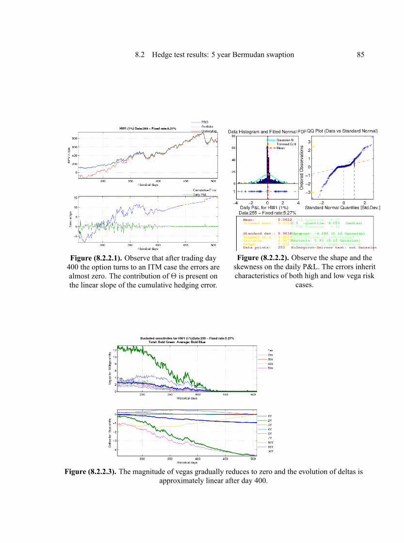
8.2 Hedge test results: 5 year Bermudan swaption 85
Figure (8.2.2.1). Observe that after trading day400 the option turns to an ITM case the errors arealmost zero. The contribution of � is present onthe linear slope of the cumulative hedging error.
Figure (8.2.2.2). Observe the shape and theskewness on the daily P&L. The errors inheritcharacteristics of both high and low vega risk
cases.
Figure (8.2.2.3). The magnitude of vegas gradually reduces to zero and the evolution of deltas isapproximately linear after day 400.

8.2 Hedge test results: 5 year Bermudan swaption 86
8.2.3 Analysis of observed data
The �rst task of our analysis is to get a feeling of how the mean reversion parameter affects the
experimental values. The normalization of the observed variables (see table (7.1.3)) facilitates a
transparent comparison along the whole set of experiments and leaves the data dependent only to
the mean reversion parameter.
The use of scatter plots indicates a positive correlation of the parameter � with the initial
option prices while this is not straightforward for the �nal hedging error. Additionally to that the
relation of mean reversion and the portfolio sensitivities is examined. The analysis takes the �aver-
age total bucketed sensitivities� into account. The scatter diagrams show signi�cant correlation of
vega sensitivity with the mean reversion parameter for ATM and OTM deals, while for delta this
holds only for ITM deals. This result was expected according to our previous comments on what
type of instruments contribute to the replication according to moneyness.
The following �gures offer a visual evaluation for the effect of the mean reversion risk on
different experimental variables.
Figure (8.2.3.1). The upper-left diagram plots all the initial option prices �PSO�. The plots that

8.2 Hedge test results: 5 year Bermudan swaption 87
correspond to �ATM�, �OTM� and �ITM� titles show only the option prices that belong to ATM,OTM and ITM cases respetively. All diagrams suggest positive correlation between prices and
mean reversion.
Figure (8.2.3.2). We evaluate the groups of the previous �gure (8.2.3.1) w.r.t. �. The silhouettesindicate the formation of compact clusters with respect to the mean reversion. We observe that the
ATM and ITM cases have a bit higher silhouettes than the ITM cases.
Figure (8.2.3.3). The scatter diagrams show that the �nal hedging error (herein F.H.Error) doesnot indicate any type of correlation to the mean reversion risk. Compare this fact the scatter
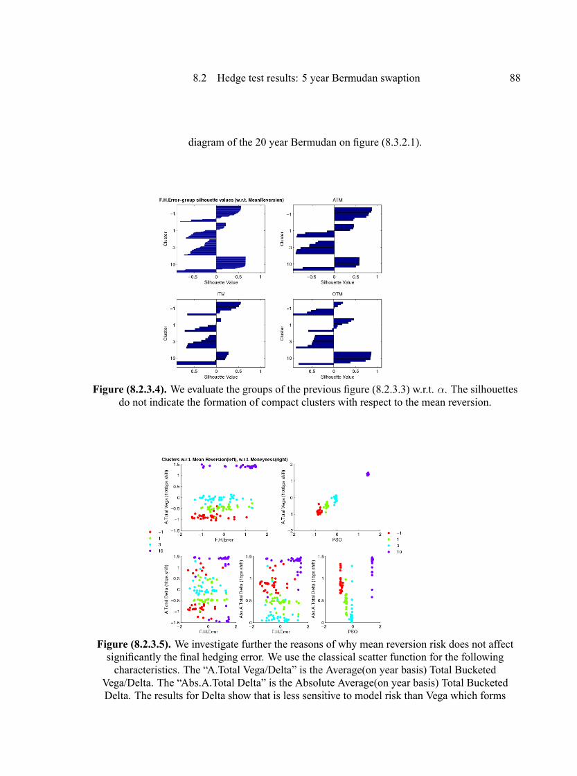
8.2 Hedge test results: 5 year Bermudan swaption 88
diagram of the 20 year Bermudan on �gure (8.3.2.1).
Figure (8.2.3.4). We evaluate the groups of the previous �gure (8.2.3.3) w.r.t. �. The silhouettesdo not indicate the formation of compact clusters with respect to the mean reversion.
Figure (8.2.3.5). We investigate further the reasons of why mean reversion risk does not affectsigni�cantly the �nal hedging error. We use the classical scatter function for the followingcharacteristics. The �A.Total Vega/Delta� is the Average(on year basis) Total Bucketed
Vega/Delta. The �Abs.A.Total Delta� is the Absolute Average(on year basis) Total BucketedDelta. The results for Delta show that is less sensitive to model risk than Vega which forms

8.2 Hedge test results: 5 year Bermudan swaption 89
compact clusters and shows a positive correlation with the mean reversion parameter.
Figure (8.2.3.6). We evaluate then �A.Total Vega� groups of the previous �gure (8.2.3.1) w.r.t. �.The �gure shows only the silhouettes for the Average Total Bucketed Vega w.r.t. mean reversion.The ATM and OTM values form compact clusters w.r.t. � parameter. This is because the hedging
positions are mainly taken on vanilla swaptions.
Figure (8.2.3.7). We evaluate then �Absolute.A.Total Delta� groups of the previous �gure(8.2.3.1) w.r.t. �.The �gure shows only the silhouettes for the Average Total Bucketed Delta w.r.t.mean reversion. The � parameter is important for the ITM deals since the hedging portfolio is
almost composed from positions on vanilla swaps.

8.3 Hedge test results: 20 year Bermudan swaption 90
8.3 Hedge test results: 20 year Bermudan swaption
The last part of our experiments include the hedge test on 20 year deals as we have described at
the beginning of the chapter. The number of simulation paths is set to 50K. We have chosen only
3 market scenarios starting at 0 and 510 trading day from our historical data. We will consider to
test only ATM cases once they are more interesting from a model risk point of view. Therefore, in
total we perform 8 hedge tests.
For computational reasons the yield curve will depend only on the 5, 10 and 30 years swap
rates and the model will be calibrated to the 3 vanilla swaptions that expire at the �rst, tenth and
twentieth exercise date of the Bermudan swaption respectively. Hence we will have 3 bucketed
deltas and vegas.
This amount of experiments is statistically not important. Even though, we include the results
to give a small example of how the model risk may appear on options of long maturity. The results
show that the presence of model risk on these deals is much higher than the short maturity deals.
The mean reversion risk proves to affect all the experimental values in comparison to the 5 years
options. Below we provide information all the �experimental cases�. In appendix (H) the initial
option price and the hedging error of each hedge test are listed in tables. As we can see from the
tables the biggest contribution to the �nal hedging error comes from the initial option premium
which is invested in cash at the beginning of the hedging. That means that the range of the �nal
hedging error is mainly formed from the initial mispricing and not from the hedge test itself.

8.3 Hedge test results: 20 year Bermudan swaption 91
(A) ObservationnScenario 0 510Initial Option Price 422.9895 458.5873
Range 54.047 59.235St.Deviation 23.23469 25.47681
(B) ObservationnScenario 0 510Final Hedging Error 8.729 -23.477
Range 71.596 49.966St.Deviation 31.20136 21.43587
Table 8.6. The table (A) shows the initial derivative price and the table (B) shows the �nal hedgingerror.
Figure (8.3.1.1). The �gure shows the NPVs ofan ATM 20 years Bermudan and its related
hedging errors.
Figure (8.3.1.2). The daily errors of thereplication form the daily P&L distributionof this experiment. It is interesting to com-pare the size of the standard deviation of this
distribution to the deviation in �gure(8.2.1.5)
8.3.1 High model risk deals
Here we present one of the 8 experiments on 20 years Bermudan swaptions. The experiment uses
the same market scenario with that in �gure (8.2.1.4) for the hedge test of a 5 years ATMBermudan
swaption. The similarity of the results will be enough to imply that both the 5 and 20 years deal
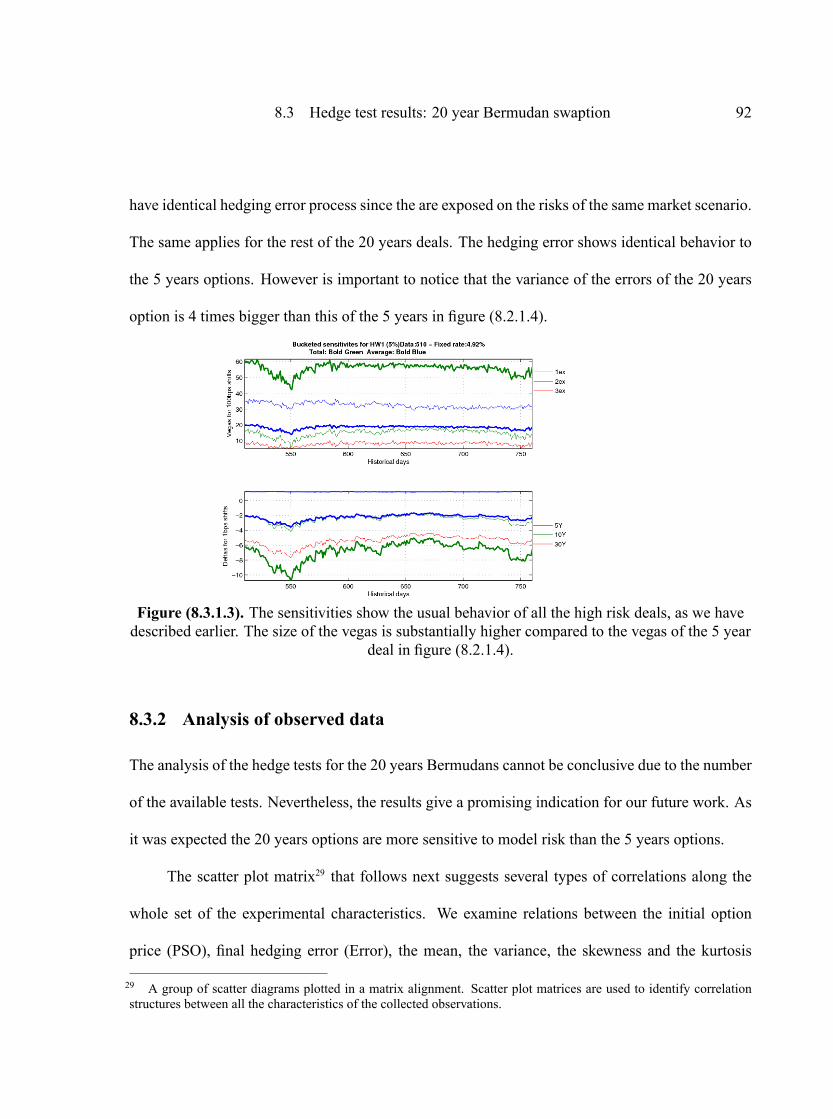
8.3 Hedge test results: 20 year Bermudan swaption 92
have identical hedging error process since the are exposed on the risks of the same market scenario.
The same applies for the rest of the 20 years deals. The hedging error shows identical behavior to
the 5 years options. However is important to notice that the variance of the errors of the 20 years
option is 4 times bigger than this of the 5 years in �gure (8.2.1.4).
Figure (8.3.1.3). The sensitivities show the usual behavior of all the high risk deals, as we havedescribed earlier. The size of the vegas is substantially higher compared to the vegas of the 5 year
deal in �gure (8.2.1.4).
8.3.2 Analysis of observed data
The analysis of the hedge tests for the 20 years Bermudans cannot be conclusive due to the number
of the available tests. Nevertheless, the results give a promising indication for our future work. As
it was expected the 20 years options are more sensitive to model risk than the 5 years options.
The scatter plot matrix29 that follows next suggests several types of correlations along the
whole set of the experimental characteristics. We examine relations between the initial option
price (PSO), �nal hedging error (Error), the mean, the variance, the skewness and the kurtosis
29 A group of scatter diagrams plotted in a matrix alignment. Scatter plot matrices are used to identify correlationstructures between all the characteristics of the collected observations.

8.3 Hedge test results: 20 year Bermudan swaption 93
and the daily P&L (herein mean, std, skew and kurt respectively). The diagrams form clear types
of correlations among all the combination of variables. The same scatter matrix for the 5 years
Bermudan does not indicate signi�cant correlation structures except from the initial price of the
derivative. Furthermore the scatter plots of vega and delta are given as well. In general, all the
characteristics apart from delta indicate a strong dependence on the mean reversion risk. The
dependencies with respect to � are described on the following �gures.
Figure (8.3.2.1). The results were expected according to the previous analysis of the 5 yearsdeals. The initial option price is positive correlated to the mean reversion parameter. The higher
the � the higher the price will be.
Figure (8.3.2.2). For 20 years deals we see that the mean reversion parameter does show a
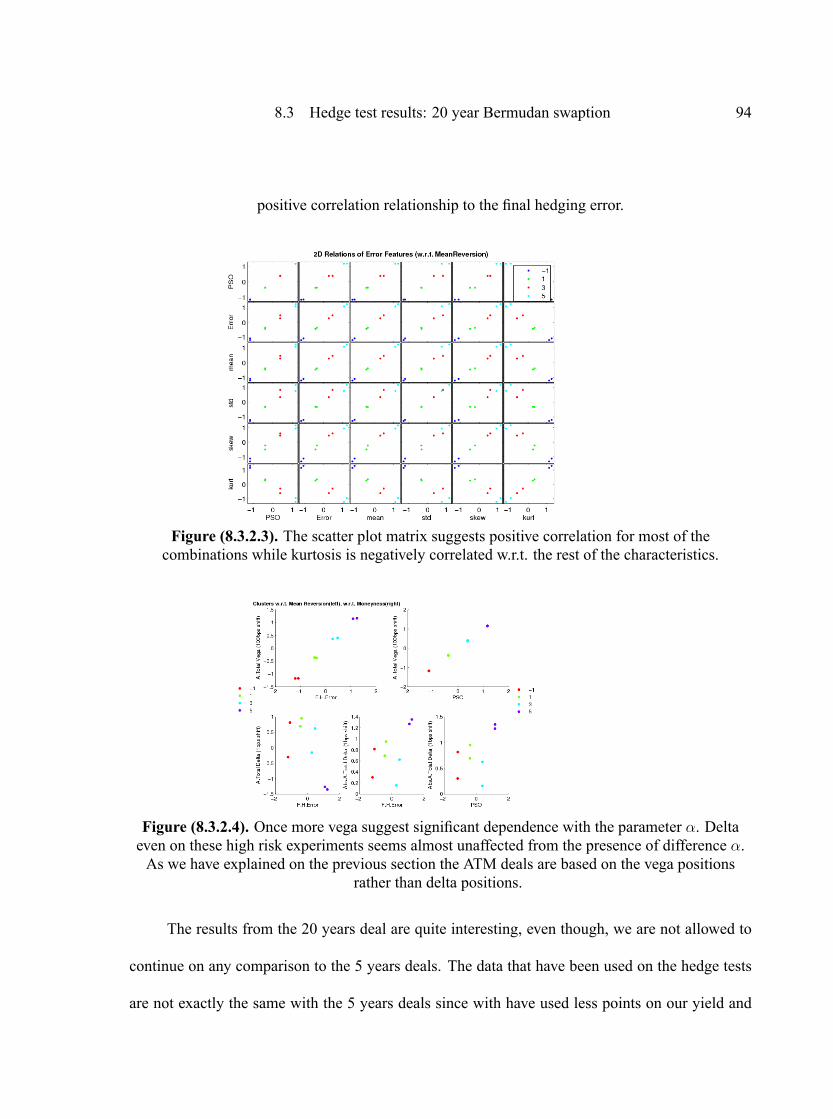
8.3 Hedge test results: 20 year Bermudan swaption 94
positive correlation relationship to the �nal hedging error.
Figure (8.3.2.3). The scatter plot matrix suggests positive correlation for most of thecombinations while kurtosis is negatively correlated w.r.t. the rest of the characteristics.
Figure (8.3.2.4). Once more vega suggest signi�cant dependence with the parameter �. Deltaeven on these high risk experiments seems almost unaffected from the presence of difference �.As we have explained on the previous section the ATM deals are based on the vega positions
rather than delta positions.
The results from the 20 years deal are quite interesting, even though, we are not allowed to
continue on any comparison to the 5 years deals. The data that have been used on the hedge tests
are not exactly the same with the 5 years deals since with have used less points on our yield and
8.4 An estimate for model risk 95
volatility term structures. As well as, the amount of the current experiments is not big enough for
further conclusions. The results have been presented to give an indication of how big the model
risk could be in longer maturity deals. These results suggest that the next work should focus more
on higher maturity deals, where the effect of the model risk will be higher.
8.4 An estimate for model risk
As we saw on the previous two sections the hedging error is distributed according to different
market factors. The unhedged error terms � and � seem to play an important role on the price
of our replicating portfolios. However the discretization results and the model error contribute
analogously to the �nal hedging error. Then, the equivalent expression of equation (3.15) for a
�V -hedging portfolio will be,
E = [�V E ]Unhedged + f�V EDgMarket +��V EMD +�V EMD;calib
�Model
The previous examples have shown that none of the terms should be ignored or considered as more
important than another. The size of each term depends on the market data and the nature of each
deal, while model risk remains a hidden part of the total error. This makes the quanti�cation of
model risk dif�cult. To achieve this it is required good understanding of the hedging procedure in
order to extract
EM =�V EMD +�V EMD;calib
out of E . The extraction of EM was illustrated with an example in �gure(7.5) where a vanilla
swaption is hedged with analytical and model pricing. This is not anymore the case for exotic
options.

8.4 An estimate for model risk 96
The easiest way of looking at model risk is to consider one �experimental case� of 4 mean re-
versions (look p.76 for terminology) . The error terms [�V E ]Unhedged and f�V EDgMarket remain the
same for the elements of one �experimental case�. On the other hand, the distribution of EM will
contribute to the deviation of the 4 �nal hedging outcomes that belong to the same �experimental
case�.
In that sense, a possible estimate for the mean reversion uncertainty is the deviation of the
EM for one experimental case with 4 different errors due to the 4 mean reversions. Meanwhile
the deviation per each experimental case differs according to moneyness and the market scenario,
hence its value differs according to the total riskiness of the deal. Thus, we need to incorporate
also this feature on our estimate.
For ATM and OTM deals vega is as measure of riskiness. Then a possible estimate of model
risk of these deals can be the ratio
Xi =Group's St.Deviation of Final Hedging ErrorGroup'sMean of Average Total Vega
Where i = 1; :::; 24 as the number of the experimental cases ( 8 data partitions � 3 levels of
moneyness ). For the calculation of the Group st.deviation and mean refer to table (8.1.3).
The histogram of all Xi may suggest an upper bound for model risk. This can be done
by setting a con�dence interval on the histogram of the Xidistribution. The right quantile of the
empirical distribution can be considered as the upper bound.
Figure (8.4.2) shows the histogram of Xi and the boxplot of the empirical distribution for
a two-sided con�dence interval of 95% applied to the results of 5 years deals. The right quantile
indicates that we are 97.5% sure that the deviation of the �nal hedging error will not exceed the
1.2 times the vega of the deal.
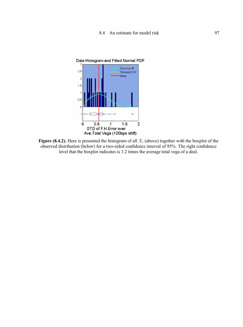
8.4 An estimate for model risk 97
Figure (8.4.2). Here is presented the histogram of all Xi (above) together with the boxplot of theobserved distribution (below) for a two-sided con�dence interval of 95%. The right con�dence
level that the boxplot indicates is 1.2 times the average total vega of a deal.
Chapter 9Conclusion
The initial plan of designing this project was to assess (or quantify) model risk for the Hull-
White one factor short rate model. Our research which has been based on hedge testing have shown
that the application of the existing model risk measures is not straightforward for unprocessed
hedging outcomes.
As a result we focused on an extensive analysis of short and long maturity deals (5 and 20
years respectively). With this analysis we managed to create a clear picture for the behavior of the
mean reversion risk of the Hull-White model on Bermudan swaptions. The conclusions upon these
analysis enable us to test a practical estimate for the mean reversion risk, which has been applied
on the set of our experiments.
9.1 Project evaluation
The �rst part of this project summarizes a long period of research related to model risk. On the
theoretical part of the thesis we provide a formal description of the related model errors. This
description aimed to present our intuition about model risk.
For the completion of our research we have designed and implemented a dynamic replicating
strategy to perform the hedging simulations. The strategy can be realized under different hedging
assumptions, hedging frequency, type of numerical sensitivities, different models and products.
98

9.1 Project evaluation 99
A signi�cant part of the thesis was spent to understand the hedging behavior of vanilla pay-
offs under different speci�cations and market scenarios. This offered signi�cant knowledge to our
team before we proceed to the �nal experiments for the model risk analysis.
The �nal results have shown that the hedging errors deviate within a range of [�45; 45] basis
points even after �ve years of hedging. Based on our hedging results we examine low and high
model risk cases. The analysis shows that the model risk on ATM and OTM deals is mainly due
to the vega of the deal while for ITM deals is due to delta. This is because when a deal is ATM or
OTM the vega is big and the hedging is based mainly on vanilla swaptions. When the deal is ITM
the hedging is based mostly on swaps.
For short maturity deals, like the 5 years Bermudan swaptions, we �nd that the �nal hedging
error is not signi�cantly correlated to the mean reversion risk. However, this is not the case for the
20y Bermudan swaptions where all the experimental parameters indicate clear forms of correlation
with respect to mean reversion parameter. The impact of the mean reversion parameter on our
results is translated to a range of 15bps for the 5 years Bermudans and 70bps for the 20 years
Bermudans, expressed in EURO.
As a part of the model risk assessment, we have also presented a possible upper bound for
model risk. This bound has shown that the model risk of the standard deviation of �nal hedging
error will not exceed the limit of 1.2 average total vega (see section (8.1.1) for terminology) of a
deal with probability 97.5%.
Additionally, the research provides evidence that the discretization and model errors of a
hedge test can be decomposed under simple assumptions in case of vanilla products. Then, if
9.2 Future work 100
indeed the hedging errors can be suf�ciently described by the equation
E = [�V E ]Unhedged + f�V EDgMarket +��V EMD +�V EMD;calib
�Model
(9.38)
there might be a possibility of decomposing the error terms of more complex products. Our main
concern is that without extracting the model error out of the observed �nal errors the quanti�cation
of mode risk will be very dif�cult to be achieved.
Methods that can implement a decomposition for equations of the form (9.38) are being used
from the neural and signal processing community from mid-90s. The common objective of these
techniques is to reproduce the original sources given a set of observations when the sources are un-
known. This is usually called from researchers as �Blind signal separation� (see Hyvärinen [2000],
Das, Routray & Dash [2007]). Several application of these algorithms can be found on magnetoen-
cephalography, sound and image processing, on mobile and wireless telecommunications
9.2 Future work
This research needs to be extended to a wider range of payoffs and models, where the effect
of model and parameter uncertainty can be different. In addition, we emphasize the absence of
volatility smile in our experiments which is something that can give us even more interesting
information.
Although the most important point that needs to be addressed, with respect to model risk, is
the application of hedge tests with different model for pricing and different for hedging. Regarding
the model for hedging, the choice is easy, while regarding the model for pricing the choice will be
more dif�cult. The problem for illiquid products is that no market price is available. The choice of

9.2 Future work 101
using a multifactor or a more complex model will only allow the comparison between two different
models and not the assessment of model risk. However, by using different model for pricing as in
�gure (7.5) we might experience bigger hedging errors than what we have seen so far. If this still
is not possible the only reasonable option, of studying model risk, is to compare the model-based
price of the derivative (or the price of its hedging portfolio) minus the derivative's payoff for deals
that have been active for an equal time period. These are certainly the most important tasks that
need to be considered in a future work.
On the other hand, another interesting topic of model risk assessment is the de�nition of
risk measures and consequently the de�nition of model risk reserves. For that reason we would
recommend to concentrate on the decomposition of the hedging and pricing errors. The use of
source decomposition algorithms might prove to be useful for that purpose. Without a precise
methodology to study the model errors the problem of model risk quanti�cation will continue
bothering our books.

References
[1] Galai, D. (1983). The Components of the Return from Hedging Options Against Stocks, Journalof Business 56 1, 45-54.
[2] Rousseeuw, P.J. (1987). Silhouettes: a Graphical Aid to the Interpretation and Validation ofCluster Analysis, Journal of Computational and Applied Mathematics, 20, 53�65.
[3] Avellaneda, M., Levy, A. and Paras, A. (1995). Pricing and Hedging Derivative Securities inMarkets with Uncertain Volatilities, Applied Mathematical Finance 2(2), 73-88.
[4] Musiela, M. and Rutkowski, M. (1997).Martingale Methods in Financial Modeling. Springer,New York.
[5] Wilmott, P., Howison, D. and Dewynne, J. (1995). The Mathematics of Financial Derivatives.Cambridge Univ. Press.
[6] Derman, E. (1996). Model risk. Risk, 9, No. 5, 34�37.
[7] Carrière, J. (1996). Valuation of early-exercise price of options using simulations and nonpara-metric regression. Insurance Math. Econom. 19 19�30.
[8] Bakshi, G., Cao, C. and Chen, N. (1997). Empirical Performance of Alternative Option PricingModels. Journal of Finance, 52, 5, 2003-49.
[9] Crouhy, M., Galai, D., Mark, R. (1998). Model risk. Journal of Financial Engineering 7, 267-288.
[10] El Karoui, N., Jeanblack-Picque, M., Shreve, S. (1998). Robustness of the Black-Scholes For-mula, Mathematical Finance, Vol. 8, No. 2, 93-126.
[11] Hunt P.J., J.Kennedy (1998). Financial Derivatives in Theory and Practice. Wiley.
[12] Basle Committee on Banking Supervision (1999). A New Capital Adequacy Framework. Bankfor International Settlements, Basle.
[13] Artzner,P., Delbaen, F., Eber, J. and Heath, D. (1999). Coherent Measures of Risk, Mathemati-cal Finance, 9, pp. 203-228.
[14] Schöbel, R., Zhu, J. (1999). Stochastic volatility with an Ornstein-Uhlenbeck process: Anextension, Europ. Fin. Review, 3:23�46.
102

References 103
[15] Hoeting, J. A., D. Madigan, A. E. Raftery, and C. T. Volinsky (1999). Bayesian Model Averag-ing: A Tutorial, Stat. Sci. 14(4), 382�417.
[16] Green, T., & Figlewski, S. (1999).Market risk and model risk for a �nancial institution writingoptions. Journal of Finance, 54, 1465�1499.
[17] Bertsimas, D, L. Kogan and A.W. Lo (2000). �When Is Time Continuous?� Journal of FinancialEconomics 55(2), 173-204.
[18] Hyvärinen, A., Oja, E. (2000), Independent Component Analysis: algorithms and applications,Neural Networks, Vol.13, pp. 411-430.
[19] Duda, R. O., Hart, P. E., Stork D. G., (2001). Pattern Classi�cation.. New York: John Wiley &Sons.
[20] Tsitsiklis, J. and Van Roy, B. (2001). Regression methods for pricing complex American-styleoptions. IEEE Transactions on Neural Networks 12 694�703.
[21] Longstaff, F. A. and Schwartz, E. S. (2001). Valuing American options by simulation: A simpleleast-squares approach. Review of Financial Studies 14 113�147.
[22] Longstaff, F. A., P. Santa-Clara, and E. Schwartz (2001). Throwing away a Billion Dollars:The Cost of Suboptimal Exercise Strategies in the Swaptions Market, Journal of Financial Eco-nomics, 62, 1, 39-66.
[23] Andersen, L. and Andreasen, J. (2001). Factor Dependence of Bermudan Swaptions: FactorFiction. Journal of Financial Economics, 62, 1, 3-37.
[24] Rebonato, R. (2001): �Managing Model Risk�. In: Alexander, C. (ed.) (2001): �MasteringRisk�, Vol. 2. 82-115.
[25] Gupta, A., and M.G. Subrahmanyam. (2001). An examination of the static and dynamic per-formance of interest rate option pricing models in the dollar cap-�oor markets. Case WesternReserve University (Working paper).
[26] Bossy, M., Gibson, R., Lhabidant, F-S., Pistre, N., Talay, D. (2001). A Methodology to An-alyze Model Risk with an Application to Discount Bond Options in a Heath-Jarrow-MortonFramework. (Working paper).
[27] Jiang, G. and Oomen, R. (2001). Hedging Derivatives Risks: A Simulation Study. (WorkingPaper).

References 104
[28] Clément, E., Lamberton, D. and Protter, P. (2002). An analysis of a least squares regressionalgorithm for American option pricing. Finance Stoch. 6 449-471.
[29] Acerbi, C. (2002). Spectral measures of risk: a coherent representation of subjective risk aver-sion. Journal of Banking and Finance, 26, pp. 1505-1518.
[30] Carr, P. and Wu, L. (2002). Static Hedging of Standard Options. (Working Paper).
[31] Föllmer, H. and Schied, A. (2002) Convex measures of risk and trading constraints. Financeand Stochastics, 6, pp. 429447.
[32] Rockafellar, R. and Uryasev, S. (2002) Conditional Value-at-Risk for General Distributions.Journal of Banking and Finance, 26, pp. 1443-1471.
[33] Chen, Z. & Epstein, L.G. (2002). Ambiguity, risk and asset returns in continuous time, Econo-metrica, Vol. 70, 4, 1403�1443.
[34] Hull, H. and Suo, W. (2002). A Methodology for Assessing Model Risk and its Application tothe Implied Volatility Function Model, Journal of Financial and Quantitative Analysis 37(2),297-318.
[35] Kerkhof, J., Melenberg, B. and Schumacher, H. (2002). Model Risk and Regulatory Capital.(Working Paper).
[36] Dudenhausen, A. (2002). Effectiveness of Hedging Strategies under Model Misspeci�cationand Trading Restrictions. Bonn Econ Discussion Papers from University of Bonn
[37] Tsanakas, A., Desli, E. (2003). Risk Measures and Theories of Choice. British Actuarial Jour-nal 9(4),.959-991.
[38] Driessen, J., P. Klaassen, and B. Melenberg. (2003). The performance of multi-factor termstructure models for pricing and hedging caps and swaptions. Journal of Financial and Quan-titative Analysis 38, 635�672.
[39] Mahayni, A. (2003), Effectiveness of Hedging Strategies under Model Misspeci�cation andTrading Restrictions. International Journal of Theoretical and Applied Finance 6, 521-552.
[40] Gobet, E., and Temam, E. (2004). Discrete time hedging errors for options with irregularpayoffs. Finance and Stochastics 5, 357�367.
[41] Björk, T. (2004). Arbitrage Theory in Continuous Time. 2nd ed.Oxford University Press.

References 105
[42] Piterbarg, V.V., (2004). Risk sensitivities of Bermuda swaptions. International Journal of The-oretical and Applied Finance, 7(4):465�510.
[43] Glasserman, P., and B., Yu, (2004). Number of Paths Versus Number of Basis Functions inAmerican Option Pricing. The Annals of Applied Probability, Vol.14.
[44] Branger, N., Schlag, C. (2004).Model risk: A conceptual framework for risk measurement andhedging (Working paper).
[45] Branger, N., Esser, A., Schlag, C. (2004). "When are Static Superhedging Strategies Optimal?"(Working paper)
[46] Kerkhof, J., (2005). Testing Hedge Effectiveness for Option Positions. Quantitative Fixed In-come Research, Lehman Brothers Int.
[47] Piterbarg, V.V., (2005). Pricing and hedging callable Libor exotics in forward Libor models.Journal of Computational Finance, 8(2).
[48] Hayashi, T., Mykland, P. (2005). Evaluating hedging errors: An aysmptotic approach.Mathe-matical Finance, Vol.15, No 2, 309-343.
[49] Gupta, A., Subrahmanyam, M. (2005). Pricing and hedging interest rate options. Evidencefrom cap��oor market. Journal of Banking & Finance 29, 701�733.
[50] Danielsson, J., Jorgensen, B., Samorodnitsky, G., Sarma, M., and de Vries, C. (2005). Subad-ditivity re-examined: The case for Value-at-Risk, Preprint, London School of Economics.
[51] Campbell, S. (2005). A Review of Backtesting and Backtesting Procedures. Board of Governorsof Federal Reserve System, Washington.
[52] Branger, N. and Mahayni, A. (2006), Tractable Hedging: An Implementation of Robust Hedg-ing Strategies, Journal of Economic, Dynamics and Control 30, 1937-1962.
[53] Cont, R. (2006). Model uncertainty and its impact on the pricing of derivative instruments.Mathematical Finance, 16, 519�547.
[54] Heyde, C., Kou, S. and Peng, X. (2006). What Is a Good Risk Measure: Bridging the Gapsbetween Data, Coherent Risk Measures, and Insurance Risk Measures, Preprint, ColumbiaUniversity.
[55] Psychoyios, D., Skiadopoulos, G. (2006). Volatility options: Hedging effectiveness, pricing,and model error. Journal of Futures Markets, 26, 1�31.
References 106
[56] Brigo, D. and Mercurio, F., (2006). Interest Rate Models: Theory and Practice. 2nd edition,Springer Finance, Heidelberg.
[57] Branger, N. and Mahayni, A. (2007). Tractable Hedging With Additional Instruments. Avail-able at: http://ssrn.com/abstract=968094
[58] Cont, R., Deguest, R., Scandolo, G. (2007). Robustness and sensitivity analysis of risk mea-surement procedures. Financial Engineering Report No. 2007-06, Columbia University Centerfor Financial Engineering.
[59] Das, N.,Routray, A., Dash, P.K. (2007), ICA Methods for Blind Source Separation of Instanta-neous Mixtures: A Case Study, Neural Information Processing, Vol. 11, No. 11.
[60] Gobet, C. (2007). Comparing conditional hedging strategies, Leuven University, (Workingpaper).
[61] Bossy, M., Gibson, R., Lhabidant, F-S., Pistre, N., Talay, D. (2007). Model misspeci�cationanalysis for bond options and Markovian hedging strategies.Working Paper.
[62] Ibragimov, R. and Walden, J. (2007). The limits of diversi�cation when losses may be large,Journal of Banking and Finance, 31, pp. 2551-2569.
[63] Sibbertsen, P., Stahl, G. and Luedtke, C. (2008). Measuring model risk. Leibniz, Hanover andUlm University - (Working Paper).
[64] Alexander, C., Kaeck, A, Nogueira, L.M. (2009). Model Risk Adjusted Hedge Ratios, TheJournal of Futures Markets, Vol. 29, No. 11, 1021�1049.
[65] Gonzalez, S.C, Hari, N. (2009). Short Rate Models. The Hull and White model. ING CMRM,CMRM Quants, TN-2009-018.
[66] Kandhai, D., Hari, N., Gonzalez, S.C. (2009). Validation of Bermudan Swaptions in Kondorand FlexING. ING CMRM, CMRM Quants, VR-2009-052.
[67] Piterbarg, V.V., Andersen, L.B.G. (2010). Bermudan swaptions and callable Libor exotics. InEncyclopedia of Quantitative Finance, Cont, R. (ed.) Wiley, 177�181
[68] Kerkhof, J., Melenberg, B. and Schumacher, H. (2010). Model risk and capital reserves, Jour-nal of Banking and Finance 34, 267-279.
Appendix AAf�ne modeling
For the short rate modeling we take as an assumption that r(t) is a martingale under a risk
neutral measure Q, which is de�ned on (;F), and its dynamics are given by
dr(t) = �(t; r(t))dt+ �(t; r(t))dW (t) (A.1)
where � and � are given a priori andW (t) is a Q-Wiener process.
De�nition 7 The instantaneous forward rate at t maturing at T is de�ned as
f(t; T ) = � @
@TlogP (t; T )
where P (t; T ) is the price of a zero coupon bond at t maturing at T .
De�nition 8 The instantaneous short rate at t is de�ned by r(t) = f(t; t).
Lemma 5 For t � s � T the zero coupon bond can be seen as
P (t; T ) = exp
��Z T
t
f(t; s)ds
�or as an expectation under a risk neutral measure Q
P (t; T ) = EQ�exp
��Z T
t
r(s)ds
�jFt�
De�nition 9 If the term structure fP (t; T ) : 0 � t � T; T > 0g has a form
P (t; T ) = eA(t;T )�B(t;T )r(t) (A.2)
where A and B are deterministic then the short rate model provides an af�ne term structure (ATS).
107
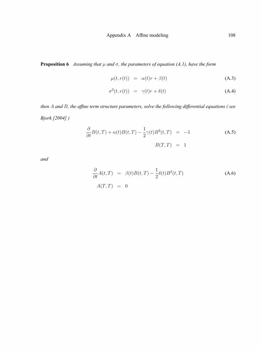
Appendix A Af�ne modeling 108
Proposition 6 Assuming that � and �, the parameters of equation (A.1), have the form
�(t; r(t)) = �(t)r + �(t) (A.3)
�2(t; r(t)) = (t)r + �(t) (A.4)
then A and B, the af�ne term structure parameters, solve the following differential equations ( see
Bjork [2004] )
@
@tB(t; T ) + �(t)B(t; T )� 1
2 (t)B2(t; T ) = �1 (A.5)
B(T; T ) = 1
and
@
@tA(t; T ) = �(t)B(t; T )� 1
2�(t)B2(t; T ) (A.6)
A(T; T ) = 0

Appendix BPiecewise constant volatility
On our setting we assume that r(t) is given as the sum of Gaussian processes xi(t) plus an
additional deterministic term which facilitates the �tting to the initial zero-coupon bond prices.
Then the r(t) dynamics for the spot measure Q0 are
r(t) =nXi=1
xi(t) + �(t)
where xi(0) = 0 and �(0) = r(0). Then we can express the dynamics of all xi(t) as system of
differential equations of the form
d!X(t) = �A
!X(t)dt+ Cd
!W (t)
where!X(t) = fx1(t); x2(t); :::; xn(t)g
0, A a strictly positive diagonal n � n matrix, C a lower
triangular n� n matrix and!W (t) = fW1(t);W2(t); :::;Wn(t)g
0a n-dimensional standard Wiener
process whileWi(t) are assumed to be i:i:d: processes. This system can be seen, according to the
representation of Dai&Singleton [2000], as
d!X(t) = �
0@ a1 0. . .
0 an
1A !X(t)dt+
0@ c1;1 0... . . .cn;1 � � � cn;n
1A d!W (t)After that we assume that the price at t of a zero-coupon bond maturing at T is
P (t; T ) = G (t; x1(t); :::; xn(t);T ) = G(t;!X(t);T ) = GT (t;
!X(t))
where GT a smooth function. Formally GT is denoted as
GT (t;!X(t)) = E0
�exp
��Z T
t
r(s)ds
�jFt�= eA(t;T )�B(t;T )
0!X(t) (B.1)
109

Appendix B Piecewise constant volatility 110
with B(t; T ) a vector of the same dimension with!X(t). Applying the multidimensional Itô rule
we get
@GT
@t�
nXi=1
aixi@GT
@xi+1
2trhC
0HC
i= rGT
GT (T;!X(T )) = 1
where H a Hessian matrix with elements Hij = @2GT
@xi@xj.
Piecewise representation
We de�ne as piecewise constant volatility �(t) the volatility of the equation (4.5) for the time
partition �n : f0 = t0 < t1 < t2 < ::: < tn�1 < tn = Tg where �(t) remains constant for the time
interval t 2 (ti�1; ti] for i = 1; :::; n. The equation (4.5) can be expressed as
dx(t) = ��x(t)dt+ �(t)dW (t)
x(0) = 0
while r(t) = x(t) + g(t) and g(0) = r(0). Then equation (B.1) can be seen as GT (ti;!X(ti)) =
eA(ti;T )�B(ti;T )0!X(ti) with
B(ti; T ) =1� exp f�(T � ti)ag
a
A(ti; T ) =1
2V (ti; tj) +
Z T
ti
g(s)ds (B.2)
where
V (ti; T ) = V (ti; tj) +n�1Xs=j
V (ts; ts+1) , 8t 2 (ti�1; ti]

Appendix B Piecewise constant volatility 111
while
V (ts; tz) =
Z tz
ts
�B(tu; T )
2�2(tk)�dtu , 8(ts; tz] 2 (tk�1; tk]
=�2(tk)
2a3�e�2aT
�eatz � eats
� �eatk + eats � 4eaT
�+ 2a (tz � ts)
�Moreover, �(t) is the term that will give the �t to the initial yield curve. This can be done by
obtaining the discount factors P(0,T) from the observed zero-coupon bond prices
P �(t; T ) = exp(A(0; T )) = exp
�1
2V (0; T )�
Z T
0
g(s)ds
�(B.3)
Using equation (B.2) we can �nd an expression for the integral
�Z T
t
g(s)ds = �Z T
0
g(s)ds+
Z t
0
g(s)ds
= lnP �(0; T )� 12V (0; T )�
�lnP �(0; t)� 1
2V (0; t)
�and �nally we �nd
A(t; T ) = lnP �(0; T )
P �(0; t)+1
2[V (t; T )� V (0; T ) + V (0; t)]
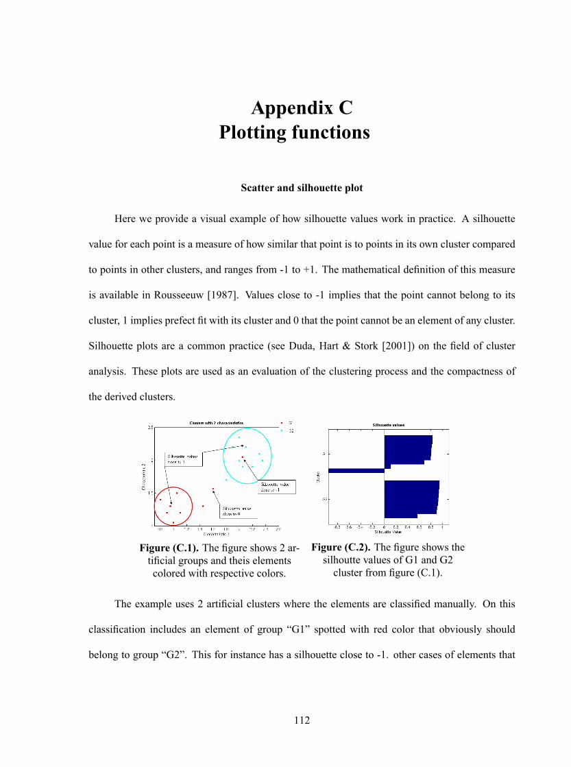
Appendix CPlotting functions
Scatter and silhouette plot
Here we provide a visual example of how silhouette values work in practice. A silhouette
value for each point is a measure of how similar that point is to points in its own cluster compared
to points in other clusters, and ranges from -1 to +1. The mathematical de�nition of this measure
is available in Rousseeuw [1987]. Values close to -1 implies that the point cannot belong to its
cluster, 1 implies prefect �t with its cluster and 0 that the point cannot be an element of any cluster.
Silhouette plots are a common practice (see Duda, Hart & Stork [2001]) on the �eld of cluster
analysis. These plots are used as an evaluation of the clustering process and the compactness of
the derived clusters.
Figure (C.1). The �gure shows 2 ar-ti�cial groups and theis elementscolored with respective colors.
Figure (C.2). The �gure shows thesilhoutte values of G1 and G2cluster from �gure (C.1).
The example uses 2 arti�cial clusters where the elements are classi�ed manually. On this
classi�cation includes an element of group �G1� spotted with red color that obviously should
belong to group �G2�. This for instance has a silhouette close to -1. other cases of elements that
112

Appendix C Plotting functions 113
might or might not belong to their group are the elements outside the groups' borders these values
will have small silhouettes or close to 0.
Signal statistics plot
This function computes and plots statistical characteristics of a signal, including the data
histogram, a �tted normal distribution, a normal distribution �tted on trimmed data, a boxplot, and
the QQ-diagram. The estimates value are printed in a panel and can be read as output. (ref. Luca
Finelli, CNL / Salk Institute - SCCN [2002]).
Figure (C.3). The signal statistics plot function shows the empirical distribution of the dailyhedging errors and QQ-diagram w.r.t. to the theoretical Gaussian distribution and other statistical
measures of the empirical distribution.
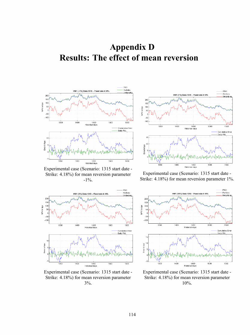
Appendix DResults: The effect of mean reversion
Experimental case (Scenario: 1315 start date -Strike: 4.18%) for mean reversion parameter
-1%.Experimental case (Scenario: 1315 start date -Strike: 4.18%) for mean reversion parameter 1%.
Experimental case (Scenario: 1315 start date -Strike: 4.18%) for mean reversion parameter
3%.
Experimental case (Scenario: 1315 start date -Strike: 4.18%) for mean reversion parameter
10%.
114

Appendix D Results: The effect of mean reversion 115
Here we compare the effect of the mean reversion parameter to the actual prices and errors
for one experimental case (the same market scenario, the same strike).
The corresponding statistics of the daily hedging errors are provided below. We assume that
the reader is already familiar with the plotting functions.
Experimental case (Scenario: 1315 start date -Strike: 4.18%) for mean reversion parameter -1%.
Experimental case (Scenario: 1315 start date -Strike: 4.18%) for mean reversion parameter 1%.
Experimental case (Scenario: 1315 start date -Strike: 4.18%) for mean reversion parameter 3%.
Experimental case (Scenario: 1315 start date -Strike: 4.18%) for mean reversion parameter 3%.

Appendix EResults: The effect of moneyness
ATM OTM
ITM
Here we show the effect of moneyness for the same market scenario and the mean reversion
parameter. The effect on the daily hedging errors is severely big.
116

Appendix E Results: The effect of moneyness 117
The corresponding statistics of the daily hedging errors are provided below. Observe the
effect of moneyness on the P&L histograms. We assume that the reader is already familiar with
the plotting functions.
ATM OTM
ITM

Appendix FResults: The effect of market risk
ATM - Scenario 1315 (the start date) ATM - Scenario 1060 (the start date)
ITM - Scenario 1315 (the start date) ITM - Scenario 1060 (the start date)
The effect of market risk is shown on the following �gures. We show an ATM (above) and
ITM (below) of the same mean reversion and moneyness on 2 different market risk scenarios.
118

Appendix F Results: The effect of market risk 119
The corresponding statistics of the daily hedging errors are provided below. We show an
ATM (above) and ITM (below) of the same mean reversion and moneyness on 2 different market
risk scenarios. We assume that the reader is already familiar with the plotting functions.
ATM - Scenario 1315 (the start date) ATM - Scenario 1060 (the start date)
ITM - Scenario 1315 (the start date) ITM - Scenario 1060 (the start date)
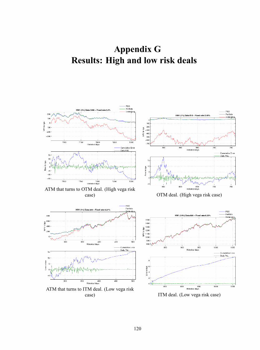
Appendix GResults: High and low risk deals
ATM that turns to OTM deal. (High vega riskcase) OTM deal. (High vega risk case)
ATM that turns to ITM deal. (Low vega riskcase) ITM deal. (Low vega risk case)
120
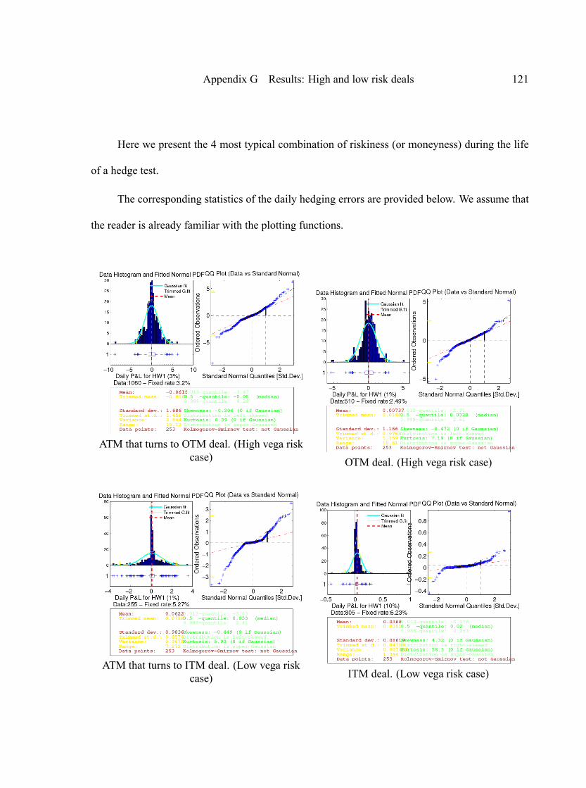
Appendix G Results: High and low risk deals 121
Here we present the 4 most typical combination of riskiness (or moneyness) during the life
of a hedge test.
The corresponding statistics of the daily hedging errors are provided below. We assume that
the reader is already familiar with the plotting functions.
ATM that turns to OTM deal. (High vega riskcase) OTM deal. (High vega risk case)
ATM that turns to ITM deal. (Low vega riskcase) ITM deal. (Low vega risk case)

Appendix G Results: High and low risk deals 122
The corresponding bucketed sensitivities are provided below. We assume that the reader is
already familiar with the plotting functions.
ATM that turns to OTM deal. (High vega risk case) OTM deal. (High vega risk case)
ATM that turns to ITM deal. (Low vega risk case) ITM deal. (Low vega risk case)
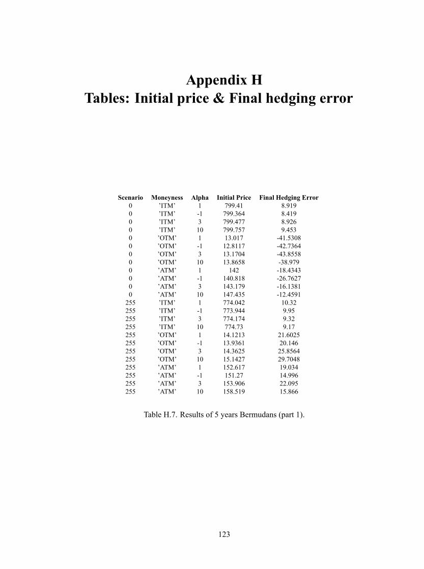
Appendix HTables: Initial price & Final hedging error
Scenario Moneyness Alpha Initial Price Final Hedging Error0 'ITM' 1 799.41 8.9190 'ITM' -1 799.364 8.4190 'ITM' 3 799.477 8.9260 'ITM' 10 799.757 9.4530 'OTM' 1 13.017 -41.53080 'OTM' -1 12.8117 -42.73640 'OTM' 3 13.1704 -43.85580 'OTM' 10 13.8658 -38.9790 'ATM' 1 142 -18.43430 'ATM' -1 140.818 -26.76270 'ATM' 3 143.179 -16.13810 'ATM' 10 147.435 -12.4591255 'ITM' 1 774.042 10.32255 'ITM' -1 773.944 9.95255 'ITM' 3 774.174 9.32255 'ITM' 10 774.73 9.17255 'OTM' 1 14.1213 21.6025255 'OTM' -1 13.9361 20.146255 'OTM' 3 14.3625 25.8564255 'OTM' 10 15.1427 29.7048255 'ATM' 1 152.617 19.034255 'ATM' -1 151.27 14.996255 'ATM' 3 153.906 22.095255 'ATM' 10 158.519 15.866
Table H.7. Results of 5 years Bermudans (part 1).
123
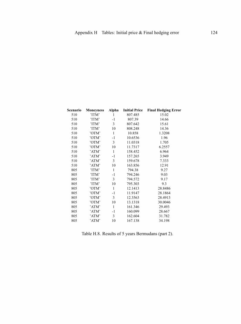
Appendix H Tables: Initial price & Final hedging error 124
Scenario Moneyness Alpha Initial Price Final Hedging Error510 'ITM' 1 807.485 15.02510 'ITM' -1 807.39 14.66510 'ITM' 3 807.642 15.61510 'ITM' 10 808.248 14.36510 'OTM' 1 10.858 1.3208510 'OTM' -1 10.6536 1.96510 'OTM' 3 11.0318 1.705510 'OTM' 10 11.7317 6.2557510 'ATM' 1 158.452 6.964510 'ATM' -1 157.265 3.949510 'ATM' 3 159.678 7.333510 'ATM' 10 163.856 12.91805 'ITM' 1 794.38 9.27805 'ITM' -1 794.246 9.03805 'ITM' 3 794.572 9.17805 'ITM' 10 795.303 9.3805 'OTM' 1 12.1413 28.8486805 'OTM' -1 11.9147 28.1864805 'OTM' 3 12.3563 28.4913805 'OTM' 10 13.1318 30.0046805 'ATM' 1 161.346 29.493805 'ATM' -1 160.099 28.667805 'ATM' 3 162.604 31.782805 'ATM' 10 167.138 34.198
Table H.8. Results of 5 years Bermudans (part 2).

Appendix H Tables: Initial price & Final hedging error 125
Scenario Moneyness Alpha Initial Price Final Hedging Error1060 'ITM' 1 849.133 3.0341060 'ITM' -1 849.099 3.061060 'ITM' 3 849.184 2.9491060 'ITM' 10 849.335 3.5451060 'OTM' 1 7.94954 -3.918731060 'OTM' -1 7.81004 -3.371311060 'OTM' 3 8.08325 -5.027011060 'OTM' 10 8.5644 -4.069181060 'ATM' 1 137.267 -3.21691060 'ATM' -1 135.86 -1.71351060 'ATM' 3 138.557 -2.68211060 'ATM' 10 143.104 2.54871315 'ITM' 1 830.184 -2.1721315 'ITM' -1 830.111 -2.1941315 'ITM' 3 830.272 -2.3671315 'ITM' 10 830.619 -1.621315 'OTM' 1 13.1907 -1.267391315 'OTM' -1 12.9547 -1.174331315 'OTM' 3 13.3622 -0.961211315 'OTM' 10 14.1057 0.11181315 'ATM' 1 150.658 1.88421315 'ATM' -1 149.332 0.62041315 'ATM' 3 151.979 0.08181315 'ATM' 10 156.651 3.5053
Table H.9. Results of 5 years Bermudans (part 3).
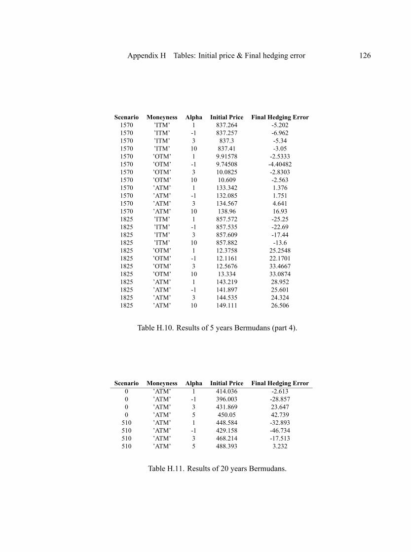
Appendix H Tables: Initial price & Final hedging error 126
Scenario Moneyness Alpha Initial Price Final Hedging Error1570 'ITM' 1 837.264 -5.2021570 'ITM' -1 837.257 -6.9621570 'ITM' 3 837.3 -5.341570 'ITM' 10 837.41 -3.051570 'OTM' 1 9.91578 -2.53331570 'OTM' -1 9.74508 -4.404821570 'OTM' 3 10.0825 -2.83031570 'OTM' 10 10.609 -2.5631570 'ATM' 1 133.342 1.3761570 'ATM' -1 132.085 1.7511570 'ATM' 3 134.567 4.6411570 'ATM' 10 138.96 16.931825 'ITM' 1 857.572 -25.251825 'ITM' -1 857.535 -22.691825 'ITM' 3 857.609 -17.441825 'ITM' 10 857.882 -13.61825 'OTM' 1 12.3758 25.25481825 'OTM' -1 12.1161 22.17011825 'OTM' 3 12.5676 33.46671825 'OTM' 10 13.334 33.08741825 'ATM' 1 143.219 28.9521825 'ATM' -1 141.897 25.6011825 'ATM' 3 144.535 24.3241825 'ATM' 10 149.111 26.506
Table H.10. Results of 5 years Bermudans (part 4).
Scenario Moneyness Alpha Initial Price Final Hedging Error0 'ATM' 1 414.036 -2.6130 'ATM' -1 396.003 -28.8570 'ATM' 3 431.869 23.6470 'ATM' 5 450.05 42.739510 'ATM' 1 448.584 -32.893510 'ATM' -1 429.158 -46.734510 'ATM' 3 468.214 -17.513510 'ATM' 5 488.393 3.232
Table H.11. Results of 20 years Bermudans.