assessment of global climate change impacts on labour
TRANSCRIPT

Assessment of global
climate change impacts
on labour productivity
Draft, do not circulate April 2019
Simon Gosling
Jamal Zaherpour
Wojtek Szewczyk

Abstract
This study assesses the impact of climate change on outdoor labour productivity at the
regional-scale and across the globe. It uses five impact models that describe observed
relationships between labour productivity and temperature, with climate model
simulations from five Global Climate Models (GCMs) under a high emissions scenario
(RCP8.5), i.e. 25 climate-impact model combinations. To the authors' best knowledge
this is the first assessment of the heat stress and labour productivity to use multiple
impact models with multiple climate models. Impacts are estimated for the end of the
century (2070-2099) and near-term (2021-2050), relative to present-day (1981-2010).
Impacts are assessed without adaptation.
Globally, at the end of the century, the spread in the magnitude of decline in labour
productivity across all 25 climate model-impact model combinations is 2-21%.
The impacts of climate change are felt heterogeneously across the globe. At the end of
the century the greatest impacts are projected for Mexico, Central America and the
Caribbean, and South Africa, where the spreads are 3-32%, 2-32% and 3-31%
respectively. The UK and Ireland, and northern Europe, experience the lowest impacts:
0-11% and 0-13% respectively.
Economic implications assessed under a static-comparative framework indicate that
mean annual global GDP losses could reach 0.2% in the 2030s and 0.6% by the end of
the century. The respective welfare losses are estimated at 0.3% and 1%, respectively.
The mean values hide significant heterogeneity across global regions, socio-economic
characteristics and the 25-member ensemble of impact projections.
An important conclusion is that the magnitudes of climate uncertainty and impact model
uncertainty are comparable for most regions. For example, for India at the end of the
century, for one impact model the spread of the decline in labour productivity is 13-22%
across climate models; whilst for one climate model, the spread is 3-27% across different
impact models. For several regions of the globe, impact model uncertainty is larger than
climate model uncertainty. It is strongly recommended, therefore, that future
assessments use multiple impact models to sample some of the range in uncertainty that
can arise from using different impact models.

i
Contents
Abstract ............................................................................................................... 2
1 Introduction ...................................................................................................... 3
2 Methods ........................................................................................................... 5
2.1 Overall approach ......................................................................................... 5
2.2 Climate models ........................................................................................... 5
2.3 Calculating WBGT ........................................................................................ 5
2.4 Impact models ............................................................................................ 6
2.5 Population data ........................................................................................... 9
2.6 Impact model evaluation ............................................................................ 10
3 Results ........................................................................................................... 11
3.1 Outdoor labour productivity ........................................................................ 11
4 Economic implications ...................................................................................... 15
4.1 The economic model .................................................................................. 15
4.2 Integration with economic model ................................................................. 15
4.3 Economic results ....................................................................................... 16
5 Discussion ...................................................................................................... 22
5.1 Selection of impact models ......................................................................... 22
5.2 Calculation of WBGT ................................................................................... 22
5.3 Economic analysis ...................................................................................... 23
6 Conclusions .................................................................................................... 24
References ......................................................................................................... 25
7 Appendix: Description of the CAGE-GEME3 model ................................................ 28
List of abbreviations and definitions ....................................................................... 32

3
1 Introduction
Climate conditions have an influence on the productivity of workers. Empirical evidence
from ergonomics studies show that most forms of human performance, hereafter referred
to as labour productivity, generally deteriorate under increasing air temperature beyond
a threshold (Hancock et al., 2007; Hancock and Vasmatzidis, 2003; Pilcher et al., 2002;
Ramsey and Morrissey, 1978; Witterseh et al., 2004). Wet Bulb Globe Temperature
(WBGT), instead of dry-bulb air temperature, is normally used when assessing the
relationship between temperature and labour productivity (Budd, 2008).
Evidence for the detrimental effects of increasing temperature on labour productivity are
largely from studies conducted within specific working environments, involving office,
factory, or outdoor workers respectively (e.g. Federspiel et al., 2002; Jeremiah et al.,
2016; Lin and Chan, 2009; Link and Pepler, 1970; Niemelä et al., 2002; Niemelä et al.,
2001). There has so far been no effort to design a study that provides empirical evidence
for changes in labour productivity with temperature across multiple working
environments, locations and countries, using a consistent methodology.
Despite the well-known association between increasing temperature and declining labour
productivity, there have been few assessments of the impact of climate change on labour
productivity, which combine climate projections with exposure response functions (ERFs)
that relate changes in labour productivity to WBGT. Some studies have used ERFs
derived from empirical studies in distinct locations (Kjellstrom et al., 2009; Kjellstrom et
al., 2013), whilst others have used ERFs developed from meta-analyses (Burke et al.,
2015; Hsiang, 2010). In the latter case, the ERF was derived from a meta-analysis of 22
ergonomics studies by Pilcher et al. (2002).
Zivin and Neidell (2015) explore the effects of high temperature on the optimal allocation
of time for individuals. The rationale is that higher temperatures can affect the optimal
decision regarding the allocation of overall time between labour and leisure, in the edn,
leading to productivity losses. That scheme has been used in the US study of climate
impacts of Hsiang et al. (2017). The recent analysis of the Climate Impact Risk
Assessment 2 (CIRA2) project of the US EPA (Martinich and Crimmins, 2019) follows a
similar methodology based on the optimal allocation of time, based also on the analysis
of Zivin and Neidell (2015).
Regarding global estimates of labour productivity and climate change, Takakura et al.
(2017) compute the cost of preventing heat-related illness when the recommended
breaks to reduce the effects of high temperatures are strictly followed. The
recommended breaks depend on the work intensity and a measure of heat stress, which
depends both on temperature and precipitation. The authors consider that all sectors of
the economy are affected. The losses in terms of lower labour are translated into GDP
losses with the use of a Computable General Equilibrium (CGE). With a dynamic
framework, where economies and population growth, they conclude that under a high
emission scenario the global losses could range between 2.6 and 4% of GDP. Those
losses would become much less under the 2C scenario, estimated at 0.5%.
A key feature of this study was setting up an ensemble of several published ERFs and
various climate models. The ensemble allowed to critically evaluate the utility of different
impact models that relate WBGT to labour productivity loss for estimating climate change
impacts on labour productivity. The exercise can be viewed as a model inter-comparison
sensitivity analysis which illustrates performance of the different impact models when
used with a consistent climate signal. Further, thanks to use of the numerous climate
models, the results also illustrate behaviour of the impact models under different future
climate paths, to provide a measure of climate uncertainty implications on labour
productivity.
With exception to Burke et al. (2015) and Houser et al. (2015), climate model
uncertainty has been relatively under-sampled in climate change impact assessments for
labour productivity. The number of climate models employed in other assessments

4
include: 1 (Dunne et al., 2013; Kjellstrom et al., 2016; Kjellstrom et al., 2013), 2
(Kjellstrom et al., 2009) and 3 (Kjellstrom et al., 2014). Estimates of the impacts of
climate change have been shown to be highly sensitive to the driving climate data from
climate models so it is important that this source of uncertainty is adequately accounted
for. No previous studies have accounted for impact model uncertainty, however, i.e. the
application of multiple impact models/ERFs for estimating impacts – the assessment
presented here is the first.
In this study the economic welfare effects of declining labour productivity are estimated
with the CGE Model, CAGE (Climate Assessment General Equilibrium). The CGE analysis
follows a static comparative approach (as in e.g. Aaheim et al., 2012; Hertel et al. 2010;
and Ciscar et al. 2012), estimating the counterfactual of future climate change (2030s
and 2080s) occurring under current socioeconomic conditions. Therefore, the climate
shock-induced changes occur as if in the economy of today.
The document is organised in five additional sections. Section 2 presents the
methodology of the study. Section 3 analyses the labour productivity results, while
section 4 discusses the key aspects of the methodology affecting the results. Section 5
focuses on the economic analysis of the impacts due to labour productivity changes.
Finally, Section 6 concludes with the main take home messages.
5
2 Methods
2.1 Overall approach
The study used simulations of climate variables from 5 different GCMs to compute daily
outdoor WBGT, for the period 1981-2100, on a 0.5° grid across the globe. The WBGT
estimates were then used as input to five separate labour productivity-WBGT ERFs to
compute daily declines in labour productivity for outdoor workers respectively on the
grid. This was done for the following time periods:
• Present-day: 1981-2010
• Near-term: 2021-2050
• End of the century: 2070-2099
The difference in labour productivity between the present period and the climate change
period was calculated and represents changes in labour productivity attributable to
climate change. Data on present-day population for each grid cell was used to calculate
the population-weighted mean regional difference (from present) in outdoor daily
average labour productivity due to climate change, for each impact model and GCM.
2.2 Climate models
The study provides a comprehensive assessment of the sensitivity of labour productivity
impacts to climate model uncertainty by computing impacts with five GCMs (HadGEM2-
ES GCM, IPSL-CM5A-LR, MIROC-ESM-CHEM, GFDL-ESM2 and NorESM1-M), all run under
a high emissions scenario (RCP8.5). The choice of the emission scenario allows to
consider impacts at higher warming levels which typically exceed 3oC warming at the end
of the current century. This set of GCMs has been used in numerous impact assessments
as part of the Intersectoral Impact Model Intercomparison Project (ISIMIP) to
demonstrate the spread in impacts that can arise from climate modelling uncertainty
(Warszawski et al., 2014).
The climate variables from each GCM were bias-corrected towards an observation-based
dataset (Weedon et al., 2011), using an established method (Hempel et al., 2013),
specifically designed to preserve long-term trends in temperature projections to facilitate
climate change impact assessments. The GCM data could therefore be used for the
present-day and future time periods in the impact assessment.
NetCDF files for daily maximum surface air temperature, daily minimum surface air
temperature, and daily mean relative humidity were downloaded for each GCM from the
Earth System Grid Foundation (ESGF), for 1981-2100.
2.3 Calculating WBGT
WBGT was calculated for outdoor (WBGTod) conditions without direct sun exposure (ie:
no short wave radiation), from indoor WBGT (WBGTid), following the approximation
described by Kjellstrom (2014):
WBGTod = WBGTid + 3⁰C
Daily WBGTid was calculated for every 0.5° grid cell from the psychrometric wet bulb
temperature (Tw) and daily maximum temperature (Tmax), following the method
described by Lemke and Kjellstrom (2012):
6
WBGTid = 0.67Tw + 0.33Tmax
Tw was not available from the GCMs so it was estimated empirically from Tmax and daily
mean relative humidity (RHmean), following Stull (2011)1:
Tw = Tmax atan[0.151977(RHmean+8.313659)1/2] + atan(Tmax+RHmean) –
atan(RHmean–1.676331) + 0.00391838(RHmean)3/2atan(0.023101RHmean) – 4.686035
2.4 Impact models
A number of past studies (e.g. Dunne et al. 2013; Burke et al. 2015; Hsiang et al. 2010)
have employed different labour productivity impact models for the purpose of labour
productivity climate change impact assessment. This study extends the relevant research
by bringing together several impact models previously used in climate change impacts
assessments.
The impact models are ERFs that describe relationships between labour productivity and
WBGT. The application of different impact models for the first time provides a
demonstration of the uncertainty in impact projections that can arise from using different
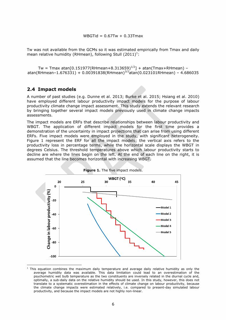
ERFs. Five impact models were employed in the study, with significant heterogeneity.
Figure 1 represent the ERF for all the impact models; the vertical axis refers to the
productivity loss in percentage terms, while the horizontal scale displays the WBGT in
degrees Celsius. The threshold temperatures above which labour productivity starts to
decline are where the lines begin on the left. At the end of each line on the right, it is
assumed that the line becomes horizontal with increasing WBGT.
Figure 1. The five impact models.
1 This equation combines the maximum daily temperature and average daily relative humidity as only the
average humidity data was available. This data limitation could lead to an overestimation of the psychometric wet bulb temperature as the two constituents are inversely related in the diurnal cycle and, optimally, a sub-daily data on the relative humidity should be used. In this study, however, this does not translate to a systematic overestimation in the effects of climate change on labour productivity, because the climate change impacts were estimated relatively, i.e. compared to present-day simulated labour productivity, and because the impact models are not highly non-linear.

7
The first impact model (model 1, black line in Figure 1) is an ERF developed by Pilcher et
al. (2002), which has been used in two recent climate change impact assessments
(Burke et al., 2015; Hsiang, 2010). The ERF is a step-function developed from a meta-
analysis of 22 studies that report associations between labour productivity and WBGT. A
more recent meta-analysis (Hancock et al., 2007) was consulted but crucially it does not
present the results as an ERF.
The ERF described by Pilcher et al. (2002) does not differentiate between the intensity of
work being undertaken by the worker – other ERFs do, e.g. the third model used in this
study (Kjellstrom et al., 2014). This is because the meta-analysis only considered how
certain types of task were effected by increases in WBGT. The ERF covers four types of
tasks: reaction time tasks, attentional or perceptual tasks (e.g., vigilance, tracking or
acuity tasks), mathematical tasks (e.g., multiplication or adding tasks, identifying lower
versus higher numbers), and reasoning, learning, or memory tasks (e.g., logic tasks,
word recall tasks). Therefore the first ERF is quite different from the other four used in
this study, because the other four have been created to specifically describe the
relationship between WBGT and physical labour. Nevertheless, the ERF defined by Pilcher
et al. (2002) is used in this study because of its application in two recent prominent
assessments of the impacts of climate change on labour productivity (Burke et al., 2015;
Hsiang, 2010). Moreover, it is the only ERF used in this study that is derived from a
systematic meta-analysis of empirical evidence published in the peer-reviewed literature.
The second impact model (blue line in Figure 1) is an ERF developed by Dunne et al.
(2013), which is based upon National Institute for Occupational Safety and Health
(NIOSH) standards and combines light, moderate and heavy labour into a single metric
by a non-linear regression equation along a continuum from 25°C to 32.2°C (Figure 1).
The decline in labour productivity is calculated as:
Decline in labour productivity (%) = 100 – (100 – (25 x max(0, WBGT – 25)2/3))
If WBGT is less than 25°C then there is no loss in labour productivity. If WBGT is greater
than 33°C, then the decline in labour productivity is 100%.
Dunne et al. (2013) notes that the ERF derives from a comprehensive attempt by NIOSH
(1986) to synthesize available knowledge on the effect of temperature on productivity in
hot and humid conditions, to yield a single recommendation on work limits with general
applicability. This resulted in the establishment of safety thresholds applicable to healthy,
acclimated labourers, sustainable over an 8-hour work period.
The second impact model displays the highest sensitivity of all the impacts models
employed in this assessment (Figure 1). Beyond the 33°C limit, the threshold implies
that no amount of labour can be safely sustained over a typical 8 hour work period.
Dunne et al. (2013) explains that this has been observed in several studies described by
NIOSH (1986) including a study of iron, ceramics, and quarry workers (Nag and Nag,
2009) that showed beyond the exercise regime of around 1 hour, the threat of heat
exhaustion and other medical effects requires a switch in the mode of labour, away from
the sustainable thresholds they define in the ERF, and towards a focus on more short-
term thermal stress accumulation where the labourer is closely monitored and allowed to
actively dissipate accumulated heat stress over long periods of recovery. As far as can be
ascertained, the original ERF applied by Dunne et al. (2013), and the method by which it
was derived, is not described in a peer reviewed journal.

8
The third impact model (red line in Figure 1) uses one of three ERFs developed by
Kjellstrom et al. (2014), which are based upon three ISO standard work intensity levels
(Parsons, 2006): 200 W (assumed to be office workers in the service industry, engaged
in light work indoors), 300 W (assumed to be industrial workers, engaged in moderate
work indoors) and 400 W (assumed to be construction or agricultural workers, engaged
in heavy work outside), and three studies that report observed declines in labour
productivity with increasing temperature (Nag and Nag, 1992; Sahu et al., 2013;
Wyndham, 1969). The ERF for heavy work only is used in this assessment because it
corresponds to the type of work conducted by the study participants that were used to
develop all the other impact models (except the first model). A limitation with the third
impact model is that the empirical evidence used to develop the ERF is from studies in
highly distinct locations, including a gold mine (Wyndham, 1969), 124 rice harvesters in
West Bengal in India (Sahu et al., 2013), and six women observed in a climatic chamber
(Nag and Nag, 1992).
To explore how impacts estimated from one of the ERFs that informed the third impact
model, compares with estimates from it, and the other impact models, the fourth impact
model is based upon empirical evidence reported by Sahu et al. (2013) (green line in
Figure 1). The authors investigated high heat exposure during agricultural tasks in India.
They observed that worker productivity reduced by approximately 5.14% for each 1°C
increase in WBGT above 26°C. Sahu et al. (2013) developed a linear regression model
that is applicable for workers who have worked for 5-hours or more. The loss in
productivity can be calculated for all WBGT values greater than or equal to 26°C and less
than 42.4°C (above 42.4°C the decline is 100%). The decline in labour productivity is
calculated as:
Decline in labour productivity (%) = 100 – ((–5.14 * WBGT) + 218)
The fifth impact model (grey line in Figure 1) uses some of the latest empirical evidence
on how labour productivity is affected by high temperatures. Li et al. (2016) observed a
0.57% decrease in productivity for every 1°C rise in WBGT above 25°C, for re-bar
workers (heavy labour) in China. The decline in labour productivity can be calculated for
all WBGT values greater than or equal to 25°C as:
Decline in labour productivity (%) = 100 – ((–0.57 * WBGT) + 106.16)
Whilst the fourth and fifth impact models are derived from empirical evidence, reported
in peer reviewed journals, they are specific to certain types of heavy labour, within
distinct climates, and with particular workers. In contrast, the first and third impact
models were derived from multiple sources of empirical evidence.
The present assessment assumes that relationships between WBGT and labour
productivity observed at the local scale, for distinct locations, types of labour and specific
individuals (e.g. 16 rebar workers in China (Li et al., 2016)), can be scaled-up for all
types of labour, the general population, and across the globe. Thus it is assumed that the
estimated impacts for outdoor labour productivity are applicable to all economic sectors
that involve moderate to intense outdoor working, including agriculture and construction.
In order to allow implementation of the impact models until the end of the current
century when the temperature increase reaches beyond 3oC, some of the ERFs were
extended beyond their calibration range. Extrapolation of Models 4 and 5 was
necessitated by the fact that in practice, labour productivity would decline further beyond
the upper temperature of the calibration limit – stopping at the calibration limit would
9
likely have underestimated the effect of WBGT on labour productivity loss. It is for this
reason that previous climate change health studies have extrapolated temperature-
health relationships beyond the empirical calibration limits (e.g. Gasparrini et al. 2017;
Dessai 2003; Gosling et al. 2009,2016).
Model 4 (Sahu et al. 2013) was calibrated between 26-32°C and extrapolated here to
100% decline in labour productivity, which occurs at 42.4°C, for the same reasons as
outlined for Model 5. Inspection of Figures 3 and 4 from Kjellstrom et al. (2014) suggests
that linear extrapolation of the linear function from Sahu et al. (2013) would still broadly
follow the S-shape of other functions however, so it is likely that any difference in labour
productivity loss relative to using an S-function is minor. Model 5 (Li et al., 2016) was
extrapolated beyond its calibration limits (25-29°C), assuming a linear growth, because
there was no evidence to indicate the shape of an S-curve for this study. The assumption
of the linear growth beyond 29°C built on other climate change impact studies (e.g.
Hsiang et al. 2010) which have used linear functions up to over 35°C.
Nonetheless, as the true relationships could be S-shaped, it is possible that labour
productivity loss is still underestimated. Other factors that could mean the impacts of
WBGT on labour productivity are underestimated include the effects of an ageing
population and population general health (e.g. personal fitness), which were not
accounted for in the projections.
2.5 Population data
Present-day population data on a 0.5° resolution grid that matched the GCM grid was
obtained from the Socioeconomic Data and Applications Centre (SEDAC) Gridded
Population of the World (SEDAC, 2017). In line with some past climate change impact
assessments for labour productivity (e.g. Dunne et al., 2013), population remained
stationary at present-day levels under the climate change scenarios.
The gridded population data was used to calculate mean regional population-weighted
labour productivity impacts attributable to climate change. The regions and countries that
comprise them are displayed in Table 1.

10
Table 1. The regions and comprising countries that were used for the computation of mean
regional population-weighted labour productivity impacts attributable to climate change.
Region Countries included in region China China
Japan Japan
Korea Korea
Indonesia Indonesia
Russia Russia
India India
USA USA
Canada Canada
Mexico Mexico
Brazil Brazil
South Africa South Africa
UK & Ireland UK, Ireland
Northern Europe Denmark, Estonia, Finland, Lithuania, Latvia, Sweden
Central Europe (North) Poland, Netherlands, Luxembourg, Germany, Belgium
Central Europe (South) Austria, Czech Republic, France, Hungary, Romania, Slovakia, Slovenia, Croatia
Southern Europe Bulgaria, Cyprus, Spain, Greece, Italy, Malta, Portugal
Australasia Australia, New Zealand, rest of Oceania
South Asia Bangladesh, Iran, Sri Lanka, Nepal, Pakistan, rest of South Asia
Sub-Saharan Africa
Botswana, Cote d'Ivore, Cameroon, Ethiopia, Ghana, Kenya, Madagascar, Mozambique, Mauritius, Malawi, Namibia, Nigeria, Senegal, Tanzania, Uganda, South Central Africa, Central Africa, rest of Eastern Africa, Rest of South African Customs Union, Rest of Western Africa, Zambia, Zimbabwe
Rest of Europe Albania, Switzerland, Norway, Rest of Eastern Europe, Rest of EFTA, Rest of Europe
Rest of South-east Asia Cambodia, Laos, Mongolia, Malaysia, Philippines, Singapore, Thailand, Taiwan, Vietnam, Rest of East Asia, Rest of Southeast Asia, Rest of the World
Rest of Former USSR Armenia, Azerbaijan, Belarus, Georgia, Kazakhstan, Kyrgyzstan, Ukraine, Rest of Former Soviet Union
Middle East & North Africa United Arab Emirates, Bahrain, Egypt, Israel, Kuwait, Morocco, Oman, Qatar, Saudi Arabia, Tunisia, Turkey, Rest of North Africa, Rest of Western Asia
Central. America & Caribbean Costa Rica, Guatemala, Honduras, Nicaragua, Panamá, El Salvador, Rest of Central America, Caribbean, Rest of North America
Rest of South America Argentina,Bolivia, Chile, Colombia, Ecuador, Peru, Paraguay, Uruguay, Venezuela, Rest of South America
Note: The choice of regional aggregation (25 regions) was decided according to the following criteria. Firstly, the
major individual countries in the climate negotiations have been included separately; therefore Brazil, Canada,
China, India, Indonesia, Japan, Korea, Mexico, Russia, South Africa and the USA are included individually. The European Union has been split into five regions: UK and Ireland, Northern Europe, Central Europe (North), Central
Europe (South) and Southern Europe. The remaining regions have been split geographically and are Australasia,
Rest of South Asia, Rest of sub-Saharan Africa, Rest of Europe, Rest of South-East Asia, Rest of Former Soviet
Union, Middle East & North Africa, Central America & Caribbean and South America.
2.6 Impact model evaluation
The five impact models are based upon empirical evidence of associations between
labour productivity and WBGT, and/or safety thresholds for conducting work in hot and
humid environments. Thus they are conceptually different from physically based impact
models such as hydrological models and crop yield models, which tend to be based upon
model parameters that represent physical processes and therefore require calibration and
evaluation for tuning model parameters. The labour productivity models are synonymous
with other human health impact models that are not generally evaluated, such as
temperature-mortality models, which are constructed from empirical data for specific
locations, using established epidemiological statistical techniques (Baccini et al., 2008;
Gasparrini et al., 2015). Moreover, the labour productivity models cannot be evaluated
for the locations where they were derived because this would involve evaluating the
models against their training data. Furthermore, the original datasets from which the
models were derived are not readily available, which precludes an evaluation of the
impact models with techniques such as split-sample evaluation.

11
3 Results
3.1 Outdoor labour productivity
Table 1 shows regional differences (from present) in outdoor labour productivity for the
near future (2030s) and end of century (2080s) time horizons.
Table 1: Regional differences (from present) in daily minimum, average and maximum outdoor labour
productivity due to climate change, from the ensemble of 25 climate-impact models combinations.
Figure 2 shows, for the end of the century, the mean regional differences (from present)
in daily average outdoor labour productivity due to climate change. Figure 3 shows the
results for near future.
The impacts of climate change on labour productivity are larger at the end of the century
than they are in the near-term. For the three most sensitive impact models (Models 2, 3
and 4), the impacts are around 10% points larger at the end of the century than in the
near-term. For the two least sensitive impact models (Models 1 and 5), the impacts are
around 3% points larger at the end of the century.
There is large uncertainty in the impacts as a result of using different impact models. The
impacts are smallest with the two least sensitive impact models. At the end of the
century, the impact of climate change on labour productivity is typically less than a 5%
decline in all regions. The impacts are considerably larger according to the other three
impact models and are generally within the range of 10-30% declines in labour
productivity due to climate change.
min mean max min mean max
China -0.6 -3.2 -7.5 -1.7 -9.3 -19.7
South-east Asia -0.6 -3.9 -9.7 -1.5 -10.1 -24.8
South-west Asia -0.8 -4.2 -8.8 -2.3 -12.5 -24.2
India -0.6 -4.3 -9.3 -2.2 -13.1 -26.7
Indonesia -0.5 -3.4 -10.1 -1.1 -8.4 -24.9
Japan -0.4 -2.4 -5.8 -1.6 -8.1 -18.1
Korea -0.6 -3.1 -7.5 -1.6 -9.1 -19.0
Australia and Oceania -0.6 -2.8 -6.0 -1.6 -8.5 -18.3
USA -0.7 -3.5 -7.6 -2.2 -10.2 -20.5
Canada -0.4 -1.9 -5.2 -1.1 -6.9 -17.6
Mexico -1.0 -5.6 -12.8 -2.6 -15.6 -32.3
Central America and Caribbean -0.8 -5.8 -13.5 -2.1 -15.2 -31.8
South America -0.8 -3.9 -8.5 -2.2 -11.3 -22.0
Brazil -0.5 -4.8 -10.7 -2.1 -14.2 -28.9
Sub-Saharan Africa -0.7 -4.9 -11.7 -2.0 -13.8 -29.9
Middle East & North Africa -0.8 -4.2 -9.4 -2.2 -12.0 -25.2
South Africa -0.9 -4.8 -10.9 -2.9 -15.1 -31.0
Northern Europe -0.2 -0.9 -4.2 -0.4 -3.5 -12.6
UK & Ireland -0.1 -0.8 -3.4 -0.4 -2.9 -10.3
Central Europe North -0.4 -1.6 -4.7 -0.9 -5.6 -16.1
Central Europe South -0.5 -2.4 -6.6 -1.3 -7.5 -19.9
Southern Europe -0.5 -2.8 -8.1 -1.6 -8.4 -21.4
Rest of Europe -0.4 -1.9 -5.0 -1.2 -6.2 -16.9
Rest of FSU -0.5 -2.6 -6.6 -1.6 -7.8 -19.8
Russia -0.4 -1.8 -5.3 -1.0 -5.8 -17.2
Global -0.7 -3.7 -7.5 -1.9 -10.8 -20.5
Region 2030s 2080s

12
A similar degree of uncertainty regarding the productivity impacts is due to using
multiple GCMs. Moreover, the magnitudes of GCM and impact model uncertainty are
comparable for most regions. For example, for India at the end of the century, for one
impact model (Model 2) the spread of the decline in labour productivity is 13-22% across
climate models; whilst for one climate model (HadGEM2-ES), the spread in impacts is 3-
27% across different impact models.
There is significant variation in the magnitude of impact across regions at the end of the
century. The three regions that experience the largest impacts are Mexico, Central
America and the Caribbean, and South Africa, where the spread in the magnitude of
decline in labour productivity across all 25 climate-impact model combinations is 3-32%,
2-32% and 3-31% respectively. In contrast, the two regions that experience the least
impacts are UK and Ireland, and northern Europe, where the spreads of declines in
labour productivity are 0-11% and 0-13% respectively. For comparison, the spread in
impacts globally is 2-21%.

13
Figure 2. End of century mean regional differences (from present) in daily average outdoor labour productivity due to climate change.

14
Figure 3. Near future mean regional differences (from present) in daily average outdoor labour productivity due to climate change.

15
4 Economic implications
This section presents estimates of economic implications of changes in labour
productivity for near term (2030s) and end of century (2080s) scenarios. The results
reflect changes in productivity of labour in construction and agriculture sectors. The
analysis of climate impacts follows a static comparative approach, estimating the
counterfactual of future climate change occurring under the current socioeconomic
conditions. Therefore, the changes induced by climate shock would occur in the economy
as of today. The economic model is run for the full ensemble of all 25 climate-impact
model combinations. The mean, minimum and maximum estimates from the ensemble
are discussed here.
4.1 The economic model
The economic simulations have been performed with the CAGE2 Computable General
Equilibrium (CGE) model, which is a static multi-country, multi-sector CGE model of the
world economy linking the economies through endogenous bilateral trade. The CAGE
database is mainly based on the Global Trade Analysis Project (GTAP) database, version
8 (Narayanan et al., 2012). The model's overview is provided in the Appendix and the full
model description and mathematical model statement is provided in the Annex of Pycroft
et al. (2015).
4.2 Integration with economic model
The direct impact represents the productivity change of a unit of labour, and it is
integrated within production process in the economic model as the change in productivity
of labour endowment. The sectors affected by the labour productivity shocks are
construction and agriculture. In those sectors labour is subject to intensive physical work
performed outdoors. The magnitude of the economy-wide impact will depend, inter alia,
on the labour intensity of the affected sectors and the relative sizes of the sectors in the
economy.
Figure 4 summarises the shocks introduced to the CGE model, representing percentage
loss in labour productivity for the world regions (reflecting the labour productivity loss
discussed in section 3.1).
2 See Appendix. The full model description and mathematical model statement is provided in the Annex of
Pycroft et al. (2015).

16
Figure 4: Change in labour productivity (the bars represent mean values). %.
4.3 Economic results
The change in labour productivity constitutes the shock to the CAGE CGE model. The
model was solved separately for each of the 25 impact-climate model combinations, and
the results present the maximum, mean and minimum of each of the set of results.
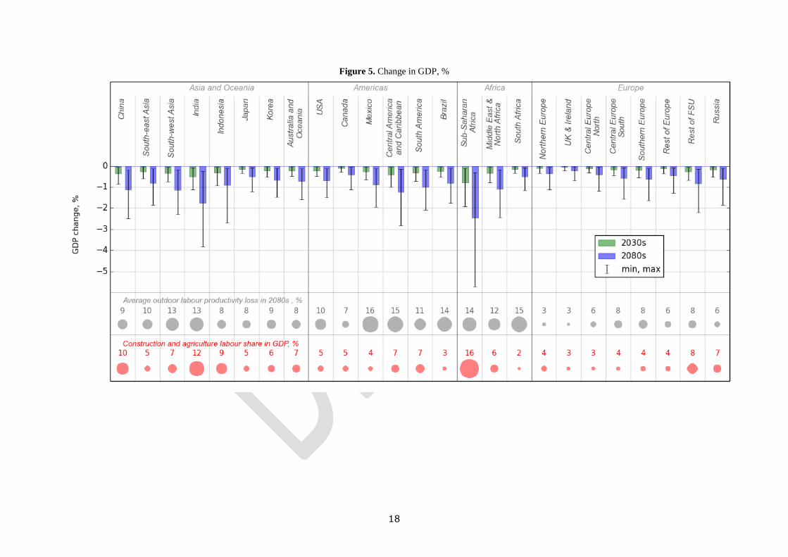
Table 2 and Figure 5 show GDP losses of the world regions for the 2030s and the 2080s.
In the 2030s the mean global GDP reduction is 0.22%, equivalent to more than €100
billion. However, there is a large range in the loss across the 25-member ensemble.
When taking the maximum estimate of loss in labour productivity from the ensemble, the
GDP reduction more than doubles compared to the mean value, to €258 billion.
The end-of-century (2080s) sees far more significant impacts of labour productivity
losses on GDP than in the near future, with a mean global GDP loss of €348 billion, up to
a maximum of €822 billion. The mean value represents 0.7% of GDP, a lower estimate
that the cost of Takakura et al. (2017). That might be due to several reasons: first, this
study assumes that only the agriculture and construction sectors are affected, rather
than all economic sectors as in the Takakura et al. study; second, this assessment is
static while that of Takakura et al. is dynamic, where GDP and population change in time.

17
Table 2: Change in GDP for different scenarios
In terms of relative GDP losses (i.e. percentage terms), Sub-Saharan Africa is the most
affected region, both in the 2030s (0.8%) and 2080s (2.5%). It is also the only region to
potentially undergo a loss greater than 2% of its GDP by the end of the century. Regions
which have more than 1% GDP loss by the 2080s are China (1.1%), India (1.8%),
Central America and Caribbean (1.2%), and Middle East and North Africa (1.1%). In
Europe the effects of climate change are greater at lower latitudes compared to higher
latitudes, e.g. at end of the century 0.2% in UK and Ireland compared with 0.6% in
Southern Europe.
In terms of absolute GDP losses (i.e. €) around 40% of global GDP losses occur in the
Americas, with a further 30% lost in Asia and Oceania, 20% in Europe, and 10% in
Africa.
min mean max min mean max min mean max min mean max
China -0.1 -0.4 -0.8 -0.2 -1.1 -2.5 -2 -11 -27 -6 -35 -78
South-east Asia 0.0 -0.3 -0.6 -0.1 -0.8 -1.8 0 -3 -7 -1 -9 -20
South-west Asia -0.1 -0.3 -0.7 -0.2 -1.1 -2.3 0 -2 -4 -1 -5 -11
India -0.1 -0.5 -1.1 -0.2 -1.8 -3.8 -1 -5 -12 -3 -19 -40
Indonesia 0.0 -0.3 -0.9 -0.1 -0.9 -2.7 0 -1 -4 0 -3 -10
Japan 0.0 -0.1 -0.3 -0.1 -0.5 -1.2 -1 -5 -13 -3 -20 -47
Korea 0.0 -0.2 -0.5 -0.1 -0.7 -1.5 0 -2 -5 -1 -6 -13
Australia and Oceania 0.0 -0.2 -0.5 -0.1 -0.7 -1.6 0 -2 -4 -1 -7 -14
USA 0.0 -0.2 -0.5 -0.1 -0.7 -1.5 -5 -27 -61 -16 -88 -188
Canada 0.0 -0.1 -0.3 -0.1 -0.4 -1.1 0 -1 -4 -1 -5 -14
Mexico 0.0 -0.3 -0.6 -0.1 -0.9 -1.9 0 -2 -6 -1 -8 -18
Central America and Caribbean -0.1 -0.4 -1.0 -0.1 -1.2 -2.8 0 -1 -3 0 -4 -10
South America -0.1 -0.3 -0.7 -0.2 -1.0 -2.1 -1 -3 -7 -2 -9 -19
Brazil 0.0 -0.2 -0.5 -0.1 -0.8 -1.8 0 -3 -6 -1 -10 -21
Sub-Saharan Africa -0.1 -0.8 -1.9 -0.3 -2.5 -5.7 -1 -4 -10 -2 -13 -29
Middle East & North Africa -0.1 -0.3 -0.8 -0.2 -1.1 -2.4 -1 -7 -15 -4 -21 -48
South Africa 0.0 -0.1 -0.3 -0.1 -0.5 -1.2 0 0 -1 0 -1 -3
Northern Europe 0.0 -0.1 -0.3 0.0 -0.4 -1.1 0 -1 -3 0 -3 -11
UK & Ireland 0.0 -0.1 -0.2 0.0 -0.2 -0.7 0 -2 -6 -1 -6 -20
Central Europe North 0.0 -0.1 -0.3 -0.1 -0.4 -1.2 -1 -6 -15 -3 -19 -54
Central Europe South 0.0 -0.2 -0.5 -0.1 -0.6 -1.6 -1 -6 -15 -3 -19 -52
Southern Europe 0.0 -0.2 -0.5 -0.1 -0.6 -1.6 -1 -7 -20 -4 -23 -62
Rest of Europe 0.0 -0.1 -0.4 -0.1 -0.5 -1.3 0 -1 -3 -1 -4 -11
Rest of FSU 0.0 -0.3 -0.7 -0.2 -0.8 -2.2 0 -1 -2 0 -3 -7
Russia 0.0 -0.2 -0.5 -0.1 -0.6 -1.8 0 -2 -6 -1 -7 -20
Global -0.04 -0.22 -0.49 -0.12 -0.70 -1.57 -19 -106 -258 -57 -348 -822
percentage change bn €
Region 2030s 2080s 2030s 2080s
18
Figure 5. Change in GDP, %

19
The magnitude of economy-wide impact will depend, inter alia, on labour productivity
loss in each of the regions (Figure 4), and on the labour intensity of the affected sectors
and their relative sizes in the economy.
The complementary information presented at the lower part of Figure 5 assists in
explaining the regional economic effects. The grey circles indicate the average labour
productivity loss in the 2080s and the red indicators show a share of each region's GDP
contributed by the affected labour in the construction and agricultural sectors.
The region with the largest GDP loss, Sub-Saharan Africa, does not experience the
biggest productivity reductions but it has a very large share of its workforce, 16%,
employed in the two affected economic sectors. Other regions with high labour
productivity losses, e.g. Mexico (16%), Central America and Caribbean and South Africa
(15%), have a much smaller proportion of their workforce employed in construction and
agriculture, hence the 'weight' placed on the productivity loss is smaller and the resulting
GDP loss is also smaller.
The welfare effects (Table 3 and Figure 6) are similar in value terms to the GDP losses,
however they are much larger when expressed in proportional terms because the
households' consumption (against which the welfare loss is measured) is only one of the
components of GDP. Taking the mean declines in labour productivity from the 25-
member ensemble, the global welfare reductions are 0.4% in the 2030s and 1.3% in the
2080s. If the maximum productivity losses are assumed, then the welfare losses are
0.9% and 2.9% respectively.
Table 3: Change in welfare for different scenarios
Regionally, the largest welfare losses are in Sub-Saharan Africa (1.4% in 2030s and
4.4% in 2080s), India (1% in 2030s and 3.4% in the 2080s), China (1% in 2030s and
3% in 2080s), and in Middle East and North Africa (0.8% and 2.4%). Other world regions
see welfare losses below 1% in the 2030s. By the end of the century, most of the regions
in the Americas and in Africa lose between 1-2% of welfare. In Europe the welfare loss is
below 1.5% with exception to Rest of the FSU where the loss is 1.8%.
min mean max min mean max min mean max min mean max
China -0.2 -1.0 -2.3 -0.5 -3.0 -6.7 -2 -11 -27 -6 -35 -78
South-east Asia -0.1 -0.4 -1.1 -0.2 -1.3 -3.3 0 -2 -6 -1 -7 -18
South-west Asia -0.1 -0.6 -1.3 -0.3 -2.1 -4.2 0 -2 -4 -1 -6 -12
India -0.1 -1.0 -2.2 -0.5 -3.4 -7.4 -1 -6 -13 -3 -20 -44
Indonesia -0.1 -0.6 -1.7 -0.2 -1.5 -4.8 0 -1 -4 0 -3 -10
Japan -0.1 -0.3 -0.7 -0.2 -1.0 -2.4 -1 -6 -14 -4 -21 -49
Korea -0.1 -0.4 -1.1 -0.2 -1.4 -3.0 0 -2 -5 -1 -6 -14
Australia and Oceania -0.1 -0.4 -0.9 -0.2 -1.4 -3.2 0 -2 -4 -1 -7 -15
USA -0.1 -0.3 -0.8 -0.2 -1.1 -2.4 -5 -28 -62 -17 -89 -190
Canada -0.1 -0.3 -0.7 -0.1 -1.0 -2.6 0 -2 -5 -1 -6 -17
Mexico -0.1 -0.5 -1.1 -0.2 -1.5 -3.2 0 -2 -6 -1 -8 -18
Central America and Caribbean -0.1 -0.7 -1.6 -0.2 -2.0 -4.5 0 -2 -4 -1 -5 -11
South America -0.1 -0.6 -1.3 -0.3 -1.9 -3.8 -1 -3 -7 -2 -10 -20
Brazil 0.0 -0.4 -1.0 -0.2 -1.4 -3.1 0 -3 -6 -1 -9 -20
Sub-Saharan Africa -0.2 -1.4 -3.4 -0.6 -4.4 -10.0 -1 -4 -11 -2 -14 -32
Middle East & North Africa -0.1 -0.8 -1.7 -0.4 -2.4 -5.4 -1 -7 -17 -4 -24 -53
South Africa 0.0 -0.2 -0.6 -0.1 -0.9 -1.9 0 0 -1 0 -1 -3
Northern Europe 0.0 -0.2 -0.7 -0.1 -0.6 -2.3 0 -1 -3 0 -3 -10
UK & Ireland 0.0 -0.1 -0.4 0.0 -0.4 -1.1 0 -2 -6 -1 -6 -19
Central Europe North 0.0 -0.2 -0.6 -0.1 -0.7 -2.1 -1 -5 -14 -3 -18 -53
Central Europe South -0.1 -0.3 -0.9 -0.2 -1.1 -3.1 -1 -6 -16 -3 -19 -55
Southern Europe -0.1 -0.3 -1.0 -0.2 -1.1 -2.9 -1 -7 -21 -4 -23 -62
Rest of Europe -0.1 -0.3 -0.8 -0.2 -1.0 -2.7 0 -1 -3 -1 -5 -12
Rest of FSU -0.1 -0.6 -1.5 -0.3 -1.8 -4.9 0 -1 -3 -1 -3 -9
Russia -0.1 -0.5 -1.2 -0.2 -1.5 -4.2 -1 -2 -7 -1 -8 -23
Global -0.1 -0.4 -0.9 -0.2 -1.3 -2.9 -19 -108 -266 -58 -355 -845
Region
percentage change bn €
2030s 2080s 2030s 2080s

20
Figure 6. Welfare change, %
21
Since welfare, as measured here, reflects changes in real consumption, it will depend not
only on the size of the productivity reduction among workers employed in construction
and agricultural sectors, but also on the share of total consumption financed from
construction and agricultural wages.
For example Sub-Saharan Africa’s mean welfare loss is 4.4% by the 2080s, which results
from 14% productivity reduction in construction and agricultural labour and from a high
share of consumption financed by labour from those two sectors (25%). By contrast,
South Africa faces a 15% reduction in outdoor labour productivity but because only 4%
of income comes from outdoor employment, the 'weight' placed on the productivity loss
is much smaller and the aggregate welfare loss is 0.9%.
It should be stressed that the reported GDP and welfare results reflect regional averages,
which is underpinned by more heterogeneous effects that vary nationally and sub-
nationally, across sectors and across demographics.

22
5 Discussion
5.1 Selection of impact models
A large spread in impacts is projected with the different impact models, for any given
climate model. This highlights the likely underestimation of impacts in earlier studies that
have used only one impact model (e.g. Burke et al., 2015; Hsiang, 2010). Whilst the
approach used in this study is not exhaustive, because not every ERF ever developed was
applied, the study does show for the first time, the choice of impact model can have a
significant effect on the projected impacts of climate change on labour productivity.
Other researchers are therefore encouraged to account for this significant source of
uncertainty in future work.
Nevertheless, it is acknowledged that more impact models could have been used, such as
those reported by Graff Zivin and Neidell (2014) and used by Houser et al. (2015).
However, a balance needs to be struck between several competing factors: the number
of impact models included, computational resources, and the form of the impact models.
This is why only five impact models were used here. More specifically, all the impact
models applied here, describe the relationship between WBGT and percentage changes in
labour productivity. The model described by Graff Zivin and Neidell (2014), for instance,
differs from these five in two fundamental ways: 1) it is based upon identifying the
incremental influence of daily maximum temperature, not WBGT; and 2) it estimates the
effects of maximum temperature on the number of minutes individuals work, not
specifically a change in productivity in percentage terms. This is no more an advantage
or a disadvantage over the approach used in the present assessment; it is a different
methodology. However, to maintain a degree of consistency between the impact models
used in the present study, only models that report changes in labour productivity in
percentage terms and with WBGT were included.
5.2 Calculation of WBGT
Daily maximum WBGT and daily minimum WBGT was calculated from daily maximum
temperature and minimum temperature respectively, with mean daily relative humidity in
both cases, because daily maximum and minimum relative humidity was not available
from the GCMs. However, this inherently assumes that the daily peaks and troughs
respectively, in temperature and humidity, occur at the same time of the day. They
could, however, occur several hours apart. The highest temporal-resolution data
available from the GCMs employed in this study was daily. It was not possible, therefore,
to estimate WBGT more precisely. An alternative approach to estimating WBGT more
precisely could involve calculating it from daily mean vapour pressure, which could be
calculated from dewpoint temperature and daily maximum temperature, following Buck
(1981). There is very little diurnal cycle in vapour pressure and so it is suitable for
calculating WBGT at maximum temperature (Eurocontrol, 2011). However, bias corrected
daily dewpoint temperature was not available from the GCMs used.
Thus there is likely to be a small error in the magnitude of daily maximum and minimum
WBGT estimated from the climate models relative to what would actually be observed. To
understand the magnitude of this error requires an evaluation using higher temporal
resolution empirical data, ideally at hourly or 15-minute resolution. The magnitude of
error could vary spatially across the globe, so the errors would need to be evaluated
across the global domain, for multiple locations, to facilitate a robust analysis. This would
require significant resource, because weather observations from multiple meteorological
stations across the globe would need to be downloaded, quality controlled, and analysed.
The magnitude of error between bias corrected simulated WBGT and observed WBGT
would also need to be compared. The variety of methods that can be used to estimate
WBGT (Lemke and Kjellstrom, 2012) would compound the evaluation further. Such an
evaluation is beyond the remit of this study. The authors are not aware of a study that
has conducted such an evaluation, so this is a worthwhile avenue for further research.

23
5.3 Economic analysis
The economic analysis benefits from the richness of the ensemble's labour productivity
results as the economic model is implemented for each of the climate-model impact-
model combinations. This rage of results provides a measure of how the uncertainty in
the climate and impact models translates into socio-economic results. Use of the
economic model allows to simulate climate-induced regional labour productivity changes
within the specific regional economic circumstances viz. bring into the analysis factors
such as the actual amount of the labour affected, relative size of the construction and
agricultural sectors, and a share of household income due to wages from those sectors.
Importance of consideration of the economic environment is demonstrated by illustrating
how a similar change in labour productivity can imply different welfare and GDP effects in
different regions.
The economic model is implemented in a static comparative mode - consistent with the
labour productivity computations – and basically answers the question 'what the current
economy would look like if the future climate occurs today?' The static approach does not
account for dynamic effects such as changes in composition of economy, changes in
population and labour characteristics or capital investment. On the other hand it allows to
avoid bringing into the analysis an additional uncertainty associated with development of
future economic projections.
Finally, the economic modelling accounts for private3 adaptation by having firms and
households reacting to changes in price signals resulting from the productivity shock. The
modelling does not account, however, for any planned adaptation or technical progress
which would alleviate negative consequences of the increased heat stress.
3 Also referred to as autonomous or automatic adaptation.

24
6 Conclusions
This is the first global-scale climate change impact assessment for labour productivity
using multiple climate models with multiple impact models. It is also the first to assess
the economic impacts in such a way.
This approach has yielded an important conclusion: impact model uncertainty and
climate model uncertainty are comparable in magnitude. Moreover, for several regions of
the globe, impact model uncertainty is larger than climate model uncertainty. It is
strongly recommended, therefore, that future assessments of both labour productivity
and its economic impacts use multiple impact models to sample some of the range in
uncertainty that can arise from using different impact models.
Climate change is associated with declines in labour productivity across the globe but the
magnitude of impact is heterogeneous. The largest impacts are seen in Mexico, Central
America and the Caribbean, and South Africa, whilst the least impacts are seen in the UK
and Ireland, and northern Europe.
The economic impacts of declining labour productivity with climate change could be
substantial. The uncertainty range is large, however. The ensemble of 25 climate-impact
models suggests a reduction in global GDP by the end of the century of between €57-822
billion.

25
References
Åkerstedt T (1998) Shift work and disturbed sleep/wakefulness. Sleep Medicine Reviews
2:117-128.
Baccini M, Biggeri A, Accetta G, Kosatsky T, Katsouyanni K, Analitis A, Anderson HR,
Bisanti L, D'Ippoliti D, Danova J, Forsberg B, Medina S, Paldy A, Rabczenko D, Schindler
C, Michelozzi P (2008) Heat Effects on Mortality in 15 European Cities. Epidemiology
19:711-719.
Buck AL (1981) New Equations for Computing Vapor Pressure and Enhancement Factor.
Journal of Applied Meteorology 20:1527-1532.
Budd GM (2008) Wet-bulb globe temperature (WBGT)—its history and its limitations.
Journal of Science and Medicine in Sport 11:20-32.
Burke M, Hsiang SM, Miguel E (2015) Global non-linear effect of temperature on
economic production. Nature 527:235–239.
Ciscar J-C, Szabó L, Van Regemorter D, Soria A (2012). The integration of PESETA
sectoral economic impacts into the GEM-E3 Europe model: methodology and results.
Climatic Change 112(1):127-142
Costa G (1996) The impact of shift and night work on health. Applied Ergonomics 27:9-
16.
Dessai S (2003) Heat stress and mortality in Lisbon Part II. An assessment of the
potential impacts of climate change. Int J Biometeorol, 48 37–44
Dunne JP, Stouffer RJ, John JG (2013) Reductions in labour capacity from heat stress
under climate warming. Nature Clim. Change 3:563-566.
Eurocontrol (2011) “Challenges of growth” environmental update study.
Federspiel CC, Liu G, Lahiff M, Faulkner D, DiBartolomeo DL, Fisk WJ, Price PN, Sullivan
DP (2002) Worker performance and ventilation: Analyses of individual data for call-center
workers. Proceedings of the Indoor Air 2002 Conference, Monterey, CA. Indoor Air 2002,
Santa Cruz, CA.
Gasparrini A, Guo Y, Hashizume M, Lavigne E, Zanobetti A, Schwartz J, Tobias A, Tong S,
Rocklöv J, Forsberg B, Leone M, De Sario M, Bell ML, Guo Y-LL, Wu C-f, Kan H, Yi S-M, de
Sousa Zanotti Stagliorio Coelho M, Saldiva PHN, Honda Y, Kim H, Armstrong B (2015)
Mortality risk attributable to high and low ambient temperature: a multicountry
observational study. The Lancet 386:369-375.
Gasparrini et al. (2017) Projections of temperature-related excess mortality under
climate change scenarios. Lancet Planet Health 1:360–367
Gosling SN, Lowe JA, McGregor GR (2009) Climate change and heat-related mortality in
six cities Part 2: Climate model evaluation, sensitivity analysis, and estimation of future
impacts. International Journal of Biometeorology 53: 31-51.
Gosling SN, Hondula D, Bunker A, Ibarreta D, Liu J, Zhang X, Sauerborn R (2016)
Adaptation to climate change: a comparative analysis of modelling methods for heat-
related mortality. Environmental Health Perspectives 087008.
Graff Zivin J, Neidell M (2014) Temperature and the Allocation of Time: Implications for
Climate Change. Journal of Labor Economics 32:1-26.
Hancock PA, Ross JM, Szalma JL (2007) A Meta-Analysis of Performance Response Under
Thermal Stressors. Human Factors: The Journal of the Human Factors and Ergonomics
Society 49:851-877.
Hancock PA, Vasmatzidis I (2003) Effects of heat stress on cognitive performance: the
current state of knowledge. International Journal of Hyperthermia 19:355-372.

26
Harrington JM (2001) Health effects of shift work and extended hours of work.
Occupational and Environmental Medicine 58:68-72.
Hempel S, Frieler K, Warszawski L, Schewe J, Piontek F (2013) A trend-preserving bias
correction – the ISI-MIP approach. Earth Syst. Dynam. 4:219-236.
Hertel TW, Burke MB, Lobell DB (2010) The poverty implications of climate-induced crop
yield changes by 2030. Global Environmental Change 20:577-585.
Houser T, Hsiang S, Kopp R, Larsen K (2015) Economic risks of climate change: an
American prospectus. Columbia University Press.
Hsiang SM (2010) Temperatures and cyclones strongly associated with economic
production in the Caribbean and Central America. Proceedings of the National Academy
of Sciences 107:15367-15372.
Hsiang et al. (2017) Estimating economic damage from climate change in the United
States. Science 356, 1362–1369
Jeremiah C, Vidhya V, Kumaravel P, Paramesh R (2016) Influence of occupational heat
stress on labour productivity – a case study from Chennai, India. International Journal of
Productivity and Performance Management 65:245-255.
Kjellstrom T, Briggs D, Freyberg C, Lemke B, Otto M, Hyatt O (2016) Heat, Human
Performance, and Occupational Health: A Key Issue for the Assessment of Global Climate
Change Impacts. Annual Review of Public Health 37:97-112.
Kjellstrom T, Kovats RS, Lloyd SJ, Holt T, Tol RSJ (2009) The Direct Impact of Climate
Change on Regional Labor Productivity. Archives of Environmental & Occupational Health
64:217-227.
Kjellstrom T, Lemke B, Otto M (2013) Mapping Occupational Heat Exposure and Effects in
South-East Asia: Ongoing Time Trends 1980-2011 and Future Estimates to 2050.
Industrial Health 51:56-67.
Kjellstrom T, Lemke B, Otto M, Hyatt O, Dear K (2014) Occupational Heat Stress
Contribution to WHO project on “Global assessment of the health impacts of climate
change”, which started in 2009. Technical Report 2014: 4. Available from:
http://climatechip.org/sites/default/files/publications/TP2014_4_Occupational_Heat_Stre
ss_WHO.pdf, ClimateCHIP = Climate Change Health Impact & Prevention.
Lemke B, Kjellstrom T (2012) Calculating Workplace WBGT from Meteorological Data: A
Tool for Climate Change Assessment. Industrial Health 50:267-278.
Narayanan, G., Badri, Angel Aguiar and Robert McDougall, Eds. 2012. Global Trade,
Assistance, and Production: The GTAP 8 Data Base, Center for Global Trade Analysis,
Purdue University
Li X, Chow KH, Zhu Y, Lin Y (2016) Evaluating the impacts of high-temperature outdoor
working environments on construction labor productivity in China: A case study of rebar
workers. Building and Environment 95:42-52.
Lin R-T, Chan C-C (2009) Effects of heat on workers' health and productivity in Taiwan.
Global Health Action 2:10.3402/gha.v3402i3400.2024.
Link J, Pepler R (1970) Associated fluctuations in daily temperature, productivity and
absenteeism. ASHRAE Transactions 76:Part II: 326-337.
Martinich J, Crimmins A (2019) Climate damages and adaptation potential across diverse
sectors of the United States. Nature Climate Change.
Nag A, Nag PK (1992) Heat stress of women doing manipulative work. American
Industrial Hygiene Association Journal 53:751-756.
Nag PK, Nag A (2009) Vulnerability to heat stress: Scenario in Eestern India. National
Institute of Ocuppational Health, Ahmedabad, India, 380016.

27
Niemelä R, Hannula M, Rautio S, Reijula K, Railio J (2002) The effect of air temperature
on labour productivity in call centres—a case study. Energy and Buildings 34:759-764.
Niemelä R, Railio J, Hannula M, Rautio S, Reijula K (2001) Assessing the effects of indoor
environment on productivity. Proceedings of the Seventh World Congress, CLIMA 2000,
Naples, Itraly.
NIOSH (1986) Criteria for a Recommended Standard: Occupational Exposure to Hot
Environments (Revised Criteria 1986). Washington DC.
OSHA (2016) Occupational Safety & Health Administration - Protective Measures to Take
at Each Risk Level.
https://www.osha.gov/SLTC/heatillness/heat_index/protective_high.html.
Parsons K (2006) Heat Stress Standard ISO 7243 and its Global Application. Industrial
Health 44:368-379.
Pilcher JJ, Nadler E, Busch C (2002) Effects of hot and cold temperature exposure on
performance: a meta-analytic review. Ergonomics 45:682-698.
Pycroft J, Abrell J, Ciscar JC (2015). The Global Impacts of Extreme Sea-Level Rise: A
Comprehensive Economic Assessment. Environ Resource Econ, DOI 10.1007/s10640-
014-9866-9
Ramsey JD, Morrissey SJ (1978) Isodecrement curves for task performance in hot
environments. Applied Ergonomics 9:66-72.
Sahu S, Sett M, Kjellstrom T (2013) Heat Exposure, Cardiovascular Stress and Work
Productivity in Rice Harvesters in India: Implications for a Climate Change Future.
Industrial Health 51:424-431.
SEDAC (2017) Gridded Population of the World (GPW), v3. NASA, USA.
Stevens RG (2016) Circadian disruption and health: Shift work as a harbinger of the toll
taken by electric lighting. Chronobiology International 33:589-594.
Stull R (2011) Wet-Bulb Temperature from Relative Humidity and Air Temperature.
Journal of Applied Meteorology and Climatology 50:2267-2269.
Takakura J, Fujimori S, Takahashi K, Hijioka Y, Hasegawa T, Honda Y, Masui T (2017)
Cost of preventing workplace heat-related illness through worker breaks and the benefit
of climate-change mitigation. Environmental Research Letters
Vetter C, Devore EE, Wegrzyn LR, et al. (2016) Association between rotating night shift
work and risk of coronary heart disease among women. JAMA 315:1726-1734.
Warszawski L, Frieler K, Huber V, Piontek F, Serdeczny O, Schewe J (2014) The Inter-
Sectoral Impact Model Intercomparison Project (ISI–MIP): Project framework.
Proceedings of the National Academy of Sciences 111:3228-3232.
Weedon GP, Gomes S, Viterbo P, Shuttleworth WJ, Blyth E, Österle H, Adam JC, Bellouin
N, Boucher O, Best M (2011) Creation of the WATCH Forcing Data and Its Use to Assess
Global and Regional Reference Crop Evaporation over Land during the Twentieth Century.
Journal of Hydrometeorology 12:823-848.
Witterseh T, Wyon DP, Clausen G (2004) The effects of moderate heat stress and open-
plan office noise distraction on SBS symptoms and on the performance of office work.
Indoor Air 14:30-40.
Zivin J F, Neidell M (2015) Temperature and the Allocation of Time: Implications for
Climate Change. Journal of Labour Economics.

28
7 Appendix: Description of the CAGE-GEME3 model
Producers seek to maximise profits subject to their production technology and the cost of
inputs. The production technology is modelled using a nested constant elasticity of
substitution (CES) function which is summarised in below.
Figure 7: Production structure in the CAGE model
Note: K-L-E refers to the capital-labour-energy bundle and K-L to the capital-labour
bundle.
As shown, output is produced by combining capital (K) and labour (L) with energy (E)
and other intermediate inputs. All combinations of inputs are treated as imperfect
substitutes, as governed by CES functions (though some are given low elasticity values
to reflect low levels of substitutability).
All commodities enter the marketplace. Production from each country can be sold either
within that country or exported. Similarly, the purchase of goods and services can be
either of domestic production or imports. Total domestic demand consists of that from
households, government, investment, intermediate inputs, and inputs for transport
margins used for trade. The extent to which this domestic demand is satisfied by
imports or domestic production is governed by a two-level constant elasticity of
substitution function reflecting the imperfect substitutability at both levels. On the lower
level, imports from different regions are combined, and on the upper level, the composite
import commodity is combined with domestic production (the Armington function,
Armington, 1969).
The economic institutions included in the model are households, government, firms and
the rest of the world. Households purchase marketed commodities at market prices,
meaning that the prices include commodity taxes. Households maximise their utility or
OUTPUT
MATERIALS
K-L
K-L-E
ENERGY Various non-energy
intermediates
Labour Capital Electricity
Fuel
Gas Coal
Petroleum

29
well-being based on their preferences and the relative prices of goods and services,
subject to their income constraints. Household consumption also has a nested structure,
with households first choosing between energy and non-energy commodities and then on
consumption within these categories. Substitutability within each nest is determined by
a constant elasticity of substitution function.
There are general constraints to the system (which are not directly considered by any of
the particular economic agents). The zero profit constraint in production is imposed as
firms are assumed to operate in a competitive environment. There are also zero profit
constraints on domestic economic institutions – households, governments and
investment – which mean that all income to institutions must be accounted for with
either spending or saving. With respect to imports and transport margins, the zero profit
conditions imply that their prices are also constrained to match their costs, inclusive of
margins and taxes, as appropriate.
The macroeconomic closure rules govern the savings-investment behaviour, aggregate
government finances, the behaviour of factor markets and the trade balance between
each country and the rest of the world. The savings-investment closure maintains a
constant volume of investment, and any change in the price of investment goods is
adjusted for by changing the value of household savings. The government closure allows
public consumption to be flexible in terms of quantity, then any additional revenue to
government raises government income, and hence raises government expenditure. In
that case, government consumption is modelled with a Leontief function, i.e. an increase
(fall) in government expenditure proportionally increases (decreases) consumption of all
commodities. The factor-market closure fixes the aggregate volume of both capital and
labour at the regional level. Both capital and labour can move between sectors, however
capital and labour are immobile across regions. Thus, returns to capital and wage rate of
labour adjust to clear the market, and the wage and capital prices are region specific.
The rest-of-the-world closure fixes the current account balance between regions at the
benchmark level, with prices adjusting to ensure that all production from each region is
either consumed domestically or exported.
Table 4: List of region-codes and geographical aggregation.
Region List of countries
China China
Japan Japan
Korea Korea
Indonesia Indonesia
Russia Russia
India India
USA USA
Canada Canada

30
Mexico Mexico
Brazil Brazil
South Africa South Africa
UK & Ireland UK, Ireland
Northern
Europe Denmark, Estonia, Finland, Lithuania, Latvia, Sweden
Central
Europe
(North)
Poland, Netherlands, Luxembourg, Germany, Belgium
Central
Europe
(South)
Austria, Czech Republic, France, Hungary, Romania,
Slovakia, Slovenia, Croatia
Southern
Europe Bulgaria, Cyprus, Spain, Greece, Italy, Malta, Portugal
Australasia Australia, New Zealand, rest of Oceania
South-west
Asia
Bangladesh, Iran, Sri Lanka, Nepal, Pakistan, rest of
South Asia
Sub-Saharan
Africa
Botswana, Cote d'Ivore, Cameroon, Ethiopia, Ghana,
Kenya, Madagascar, Mozambique, Mauritius, Malawi,
Namibia, Nigeria, Senegal, Tanzania, Uganda, South
Central Africa, Central Africa, rest of Eastern Africa,
Rest of South African Customs Union, Rest of Western
Africa, Zambia, Zimbabwe
Rest of Europe Albania, Switzerland, Norway, Rest of Eastern Europe,
Rest of EFTA, Rest of Europe
South-east
Asia
Cambodia, Laos, Mongolia, Malaysia, Philippines,
Singapore, Thailand, Taiwan, Vietnam, Rest of East
Asia, Rest of Southeast Asia, Rest of the World
Rest of
Former Soviet
Union
Armenia, Azerbaijan, Belarus, Georgia, Kazakhstan,
Kyrgyzstan, Ukraine, and other countries from the rest
of Former Soviet Union
Middle East &
North Africa
United Arab Emirates, Bahrain, Egypt, Israel, Kuwait,
Morocco, Oman, Qatar, Saudi Arabia, Tunisia, Turkey,
Rest of North Africa, Rest of Western Asia
Central.
America &
Caribbean
Costa Rica, Guatemala, Honduras, Nicaragua, Panamá,
El Salvador, Rest of Central America, Caribbean, Rest
of North America
Rest of South
America
Argentina, Bolivia, Chile, Colombia, Ecuador, Peru,
Paraguay, Uruguay, Venezuela, Rest of South America
Table 5: List of sector codes and sectoral aggregation
Aggregation Constituent sectors
Agriculture Bovine cattle, sheep and goats, horses, animal
products nec, raw milk, wool, silk-worm cocoons,
fishing
Crops Paddy rice, wheat, cereal, grains nec, vegetables, fruit,
nutsv oil seeds, sugar cane, sugar beet, plant-based
fibers, crops nec
Forestry Forestry
Coal Mining Coal
Crude Oil
Extraction
Oil
Natural Gas Gas, gas manufacture, distribution

31
Refined Oil Petroleum, coal products
Electricity Electricity
Metals Ferrous metals, metals nec, metal products
Chemicals Chemical, rubber, plastic products
Energy
Intensives
Minerals nec, paper products, publishing, mineral
products nec
Electronic
equipment
Electronic equipment
Transport
Equipment
Motor vehicles and parts, transport equipment nec
Other
Equipment
Machinery and equipment nec, manufactures nec
Consumer
Goods
Bovine meat products, meat products nec, vegetable
oils and fats, airy products, processed rice, sugar, food
products nec, beverages and tobacco products,
textiles, wearing apparel, leather products, wood
products
Construction Construction
Transport Transport nec, water transport, air transport
Market
Services
Water, trade, communication, financial services nec,
insurance, business services nec, dwellings
Non-market
Services
Recreational and other services, public administration,
Defense, Education, Health

32
List of abbreviations and definitions
ERFs: exposure response functions
ESGF: Earth System Grid Foundation
GCMs: Global Climate Models
ISIMIP: Intersectoral Impact Model Intercomparison Project
NIOSH: National Institute for Occupational Safety and Health
RCP: Representative Concentration Pathway
RHmean: daily mean relative humidity
Tmax: daily maximum temperature
Tw: psychrometric wet bulb temperature
WBGT: Wet Bulb Globe Temperature
WBGTid: indoor WBGT
WBGTod: outdoor WBGT
XX-N
A-x
xxxx-E
N-C