assessing vulnerabilities in emerging-market economies
TRANSCRIPT

Bank of Canada staff discussion papers are completed staff research studies on a wide variety of subjects relevant to central bank policy, produced independently from the Bank’s Governing Council. This research may support or challenge prevailing policy orthodoxy. Therefore, the views expressed in this paper are solely those of the authors and may differ from official Bank of Canada views. No responsibility for them should be attributed to the Bank.
www.bank-banque-canada.ca
Staff Discussion Paper/Document d’analyse du personnel 2018-13
Assessing Vulnerabilities in Emerging-Market Economies
by Tatjana Dahlhaus and Alexander Lam
2
Bank of Canada Staff Discussion Paper 2018-13
October 2018
Assessing Vulnerabilities in Emerging-Market Economies
by
Tatjana Dalhaus and Alexander Lam
International Economic Analysis Department
Bank of Canada Ottawa, Ontario, Canada K1A 0G9
ISSN 1914-0568 © 2018 Bank of Canada

i
Acknowledgements
We thank Rose Cunningham, Mark Kruger, Rhys Mendes, Gurnain Pasricha and Tatevik Sekhposyan as well as seminar participants at the Bank of Canada for useful comments and suggestions. We would also like to thank Maxim Petitclerc Gagnon for his research assistance. The views expressed in this paper are those of the authors and not necessarily those of the Bank of Canada.

ii
Abstract
This paper introduces a new tool to monitor economic and financial vulnerabilities in emerging-market economies. We obtain vulnerability indexes for several early warning indicators covering 26 emerging markets from 1990 to 2017 and use them to monitor the evolution of vulnerabilities before, during and after an economic or financial crisis. We find that different historical episodes of crises reflect different vulnerabilities in terms of their composition, buildup and responses. Nevertheless, most currency crises are generally preceded by a buildup of imbalances in the external sector followed by an increase in sovereign debt imbalances. Finally, we assess current EME vulnerabilities in our country sample and visualize them using a heat map. Bank topics: International topics; Monetary and financial indicators; Recent economic and financial developments JEL Codes: C82, F34, G01, G15
Résumé
Dans cet article, nous exposons un nouvel outil visant à surveiller les vulnérabilités économiques et financières dans les pays émergents. Nous obtenons, pour la période allant de 1990 à 2017, des indices de vulnérabilité pour plusieurs indicateurs avancés couvrant 26 marchés émergents. Nous utilisons ces indices pour suivre l’évolution des vulnérabilités avant, pendant et après une crise économique ou financière. Nous constatons que différents épisodes de crise historiques s’accompagnent de vulnérabilités différentes en ce qui a trait à leur composition, à leur intensification et aux mesures prises pour y remédier. Néanmoins, la plupart des crises monétaires sont généralement précédées d’une accumulation des déséquilibres dans le secteur extérieur suivie d’une accentuation des déséquilibres de la dette souveraine. Enfin, nous évaluons les vulnérabilités actuelles des pays émergents de notre échantillon et les illustrons au moyen d’une carte thermique. Sujets : Questions internationales; Indicateurs monétaires et financiers; Évolution économique et financière récente Codes JEL : C82, F34, G01, G15

1
1. Introduction In the last two decades, the importance of emerging-market economies (EMEs) in the global economic landscape has increased. At the same time, economic and financial ties between advanced economies and EMEs have grown stronger. The growing exposure to EMEs has increased policy-makers’ need for tools to monitor economic and financial vulnerabilities in emerging markets. The Bank of Canada defines vulnerabilities as pre-existing conditions that make the occurrence of an economic or financial crisis or stress more likely when an adverse shock hits.1 This definition is consistent with other academic literature. Unlike shocks, vulnerabilities can be assessed. This paper introduces a tool to monitor current vulnerabilities in EMEs and to assess their evolution over time. Building on research on early warning systems for crises, we define different types of EME vulnerabilities that may contribute to the amplification and propagation of shocks. We use a set of commonly used early warning indicators (EWIs) covering countries’ external, sovereign and financial sectors and construct a vulnerability index for each indicator. Specifically, we propose a distribution-based measure of vulnerabilities based on assessing the likelihood of a realization of a given EWI. We assume that a country is more vulnerable to adverse shocks if a given EWI takes on unusual values when compared with its past and country peers’ EWI values.2 We construct vulnerability indexes for eight EWIs in 26 EMEs using data starting in the early 1990s. We aggregate indexes to obtain an overall measure of vulnerability for each country or across regions. To gauge the level of economic fragility at any point in time, we construct our indexes in real time.3 The literature has established numerous potential EWIs across countries and time.4 Our paper differs from this existing literature along several dimensions. First, we provide a time-varying measure of vulnerability for each EWI and country in our sample to allow for historical comparison as well as real-time analysis. Second, our approach is purely non-parametric and does not rely on any regression analysis or structural assumptions. This is an advantage when monitoring developments in EMEs since estimates can be calculated easily, in a timely manner as data are released and without any underlying model assumptions. Our assessment of vulnerabilities is determined solely using the information contained in the distribution of vulnerabilities in a cross-country panel data set.5 Since our set of EWIs does not exhibit a time trend, the sample distribution provides a useful reference point for evaluating current economic and financial conditions. Third, given that we obtain vulnerability indexes for each EWI, we can assess the contribution
1 See Christensen et al. (2015). 2 Given the nature of some early warning indicators, they could take on unusual values during as well as before a crisis. Therefore, the vulnerability index could also be interpreted as measure of stress during times of crisis. 3 To assess vulnerabilities over our sample period up to the most recent period (2017Q4), we also construct a full-sample version of the indexes. Both approaches are explained in Section 3. 4 See Frankel and Saravelos (2012) for a detailed survey of 83 published studies over the past 60 years. 5 Although our distribution-based approach is novel, previous studies compare instances of EWI values with values during crisis episodes. Aikman et al. (2015) also take a data-driven, distribution-based approach by considering the historical distribution of risk components, that is, an aggregate of certain standardized early warning indicators.

2
of different EWIs to a country’s vulnerability. Thus, we can evaluate the role of types of vulnerabilities in the buildup, during and in the aftermath of a specific crisis. Finally, we obtain our index in real time, in the sense that we consider time-varying distributions of the indicators. To construct the vulnerability indexes, we borrow from the literature measuring macroeconomic uncertainty. We apply the uncertainty index proposed by Rossi and Sekhposyan (2015) to EWIs. In Rossi and Sekhposyan (2015), the economy is considered to be more uncertain at any given point in time when the realized forecast error of say, gross domestic product (GDP), is uncommonly large and lies at either tail of its historical distribution. We apply this concept to EWIs. An economy is considered to be more vulnerable to an adverse outcome when a given EWI takes on unusual values, i.e., the realized observation of the EWI lies in the tail of its historical cross-sectional distribution.6 Therefore, the index indicates higher levels of vulnerability whenever an EWI reaches rare values. An advantage of the framework of Rossi and Sekhposyan (2015) is that it can distinguish between realizations falling into the right or left tail of the distribution. This is particularly important in the context of vulnerabilities since those related to an EWI can be exclusively one-sided. For example, a country may be more vulnerable only when its government debt is unusually high (i.e., the observation falls into the right tail). We employ visual tools to illustrate the usefulness of our indexes in accurately reflecting the anatomy of vulnerabilities over time as well as surrounding episodes of economic or financial crisis in EMEs. However, we make no attempt to explicitly test the statistical power of our indexes in predicting the onset of crisis episodes. Instead, the value-added of our approach is that our indexes allow for efficient comparisons of vulnerabilities across EWIs and countries, and provide a way to monitor the evolution of these vulnerabilities over time and their behaviour around crises.7 Comparing the level of vulnerabilities historically, we show that the overall vulnerability of EMEs seems to be lower now than during the 1990s or during the global financial crisis of 2008–09. Further, we demonstrate the capability of our index to characterize the nature of crises by assessing the role and evolution of indicator-specific vulnerabilities. Finally, we provide a heatmap that summarizes our assessment of current vulnerabilities in the 26 EMEs in our sample.
The paper proceeds as follows. In Section 2, we discuss the EWIs that we consider and use to construct our vulnerability indexes. Section 3 explains in detail how each vulnerability index is calculated and
6 One could employ country-specific historical distributions to construct country-specific vulnerability indexes. However, the occurrence of crises (and preceding high levels of vulnerabilities) is limited in each country given the short data span available. Therefore, we cannot rely on country-specific distributions. In addition, we assume that former occurrences of crises and the associated level of high vulnerabilities in one country are potentially informative for another country in our sample. 7 Testing for the predictability of the onset of crises is only one possible aspect of analysis for a vulnerability index. Here we rather focus on how informative the index is about the patterns and evolutions of several EWIs before, during and after crises. For example, we show that vulnerabilities related to government debt are usually high during a currency crisis, while current-account-related vulnerabilities are generally elevated before.

3
illustrates this with two examples of past EME crises. It also discusses how individual vulnerability indexes are aggregated across EWIs and countries. Section 4 presents the aggregate EME vulnerability index and regional indexes. Section 5 illustrates how the approach is useful to monitor the evolution of vulnerabilities over time by assessing the indicators’ impacts on an individual country’s vulnerability level. It also analyzes the evolution of vulnerabilities around major EME crises. Finally, we provide a heat map that summarizes our current assessment of EME vulnerabilities based on individual country and indicator results. Section 6 concludes.
2. Indicators of economic vulnerabilities
As described earlier, we construct vulnerability indexes for a set of early warning indicators. We base our selection of indicators on the literature on early warning systems and previous work done by the Bank of Canada.8 Our selection of indicators reflects a broad range of potential sources of economic vulnerability, such as currency and trade imbalances, high inflation, currency misalignment and debt problems. This allows us to track a variety of potential economic and financial vulnerabilities. Our sample covers 26 EMEs from 1990Q1 to 2017Q4.
However, several practical constraints determine our choice of vulnerability indicators. First, to allow for timely policy analysis, we consider quarterly indicators that are available for a broad range of EMEs. Second, to assess its effectiveness, we construct the index over several decades to capture enough past economic crises. Third, our indicators should be comparable across countries. We therefore use indicators from international organizations such as the International Monetary Fund (IMF) and Bank for International Settlements (BIS) where possible.
We consider a set of indicators that fall into three broad categories: external sector, policy sector and financial sector. External sector indicators are related to countries’ interactions with the rest of the world: current account balances, portfolio investment liabilities, foreign exchange reserves and real exchange rates.9 Policy sector indicators relate to fiscal and monetary policy decisions that may lead to economic vulnerabilities. These indicators include inflation, government debt and fiscal balances. Financial sector indicators relate to private credit growth, although we do not include any indicators of banking sector vulnerabilities specifically.10 A detailed description of each indicator and its data source is in Appendix 1.
2.1. External sector indicators
2.1.1 Current account balances
8 See, for example, Pasricha et al. (2013). 9 In an extensive review of 83 papers, Frankel and Saravelos (2012) identify foreign exchange reserves, the real exchange rate, the current account and credit growth as the EWIs with greatest predictive power for crisis episodes. 10 The literature also considers financial sector EWIs such as short-term funding, concentration and maturity transformation to describe financial vulnerabilities. However, data coverage of those EWIs is not sufficient for our sample.

4
The current account (CA) balance reflects trade and income flows. The vulnerability is left-tailed, i.e., the larger the CA deficit, the more vulnerable a country is to a shock. A larger CA deficit is associated with negative net exports or income outflows, which must be funded either through external financing, depreciating the national currency or running down foreign assets. Large and prolonged CA deficits are therefore considered unsustainable and may lead to a balance of payments crisis.
2.1.2 Portfolio investment liabilities
This measure of capital inflows captures net non-resident purchases of a country’s debt and equity. The vulnerability is two-sided, i.e., both large increases or large decreases in capital flows can increase financial system vulnerabilities and aggravate overall macroeconomic stability. Large inflows may suggest an accumulation of large external debt and/or an asset bubble resulting in inflows becoming detached from economic fundamentals and, thus, unsustainable. Similarly, liability flows on portfolio investments that are highly negative mean that capital flight may be occurring, leading to loss in liquidity and economic confidence.
2.1.3 Foreign exchange reserves
A low reserve-to-GDP ratio leaves the economy vulnerable since it becomes more difficult to pay off foreign liabilities and fund current account deficits. This is especially true in EMEs, many of which still manage or fix their currency exchange rates. Low levels of foreign reserves can make it difficult for fixed exchange rate regimes to defend their currencies against depreciation pressures and can result in destabilizing currency revaluations. The vulnerability is therefore left-tailed.
2.1.4 Real exchange rate misalignment
We define real exchange rate misalignment as the deviation of the real effective exchange rate (REER) from its past five-year average. This vulnerability indicator is two-sided. Rapid appreciations or depreciations of a country’s exchange rate may indicate that flows of foreign funds into or out of the economy may be unsustainable. Depreciations in the exchange rate also reduce purchasing power and increase the risk of economic slowdown.
2.2 Policy sector indicators
2.2.1 Inflation
We classify inflation as a policy sector indicator because high inflation may reflect an overheated domestic economy and monetary policy mismanagement. However, in small and open EMEs, high inflation may also reflect external vulnerabilities and currency speculation via exchange rate pass-through to consumer prices. High inflation or hyperinflation reduces consumer purchasing power and liquidity in the economy, and it can lead to unanchored inflation expectations, which in turn increase the risk of economic and political destabilization. We assume this vulnerability to be right-tailed. Although persistent disinflation or deflation may also reflect economic vulnerabilities by causing economic stagnation and higher real debt

5
burdens, these problems have been less prevalent in EMEs, which have most often struggled to reach low and stable inflation.11
2.2.2 Government debt
As the government debt-to-GDP ratio increases, it becomes harder for governments to service and roll over their debt, increasing the risk of default. Moreover, governments may have to enact austerity measures to service their debt, which may trigger an economic slowdown, and the costs of borrowing may increase if the current debt load is already high. Government debt is therefore a right-tailed indicator of vulnerability.
2.2.3 Fiscal balances
Sustained fiscal deficits are an indicator of economic vulnerability because deficits must be financed by increasing debt, raising taxes or cutting expenditures, which may cause an adverse shock to economic activity. High levels of government spending may also trigger an economic slowdown by crowding out private investment. Finally, high deficits leave economies more vulnerable to interest rate risk, particularly in the recent environment of normalization from historically low rates. We therefore consider this vulnerability to be left-tailed.
2.3 Financial sector indicators
2.3.1 Private credit growth
We use the year-over-year growth rate of credit to the private non-financial sector as an indicator of financial system vulnerability.12 The private non-financial sector includes households and private non-financial corporations. High credit growth may indicate a credit bubble or unsustainable private debt levels, leaving economies more exposed to interest rate risk, similar to public sector deficits. As such, we consider this vulnerability to be right-tailed.13 We consider the growth rate of credit because it is a commonly used indicator in previous literature. Moreover, other credit measures such as credit-to-GDP ratios and gaps may reflect structural differences in countries’ financial systems rather than economic vulnerabilities.
11 Given the prevalence of high inflation in EMEs over our sample period, considering the left tail of the inflation distribution may falsely attribute times of low and healthy levels of inflation to times of increased vulnerabilities. 12 Although our credit indicator excludes leverage within financial institutions, it is still considered a financial system vulnerability in that it reflects only developments in the financial sector and not the real economy. 12 Although our credit indicator excludes leverage within financial institutions, it is still considered a financial system vulnerability in that it reflects only developments in the financial sector and not the real economy. 13 A possible amendment would be to also consider credit contractions. However, this is sometimes a positive indication that banks are sorting out problems in their loan portfolios.

6
3. The vulnerability index
In this section, we outline our approach for creating the index of economic vulnerabilities using illustrative examples based on two EWIs: portfolio flows and government debt (discussed in Section 2).
3.1 Methodology
We employ Rossi and Sekhposyan’s (2015) macroeconomic uncertainty index in the context of economic vulnerabilities. Our index compares the realization of a given EWI with an empirical distribution of observations for that EWI. This distribution is cross-sectional and can be either in real time or based on the full sample. It reflects the overall experience of EMEs. For example, if the most recent observation of a country’s current account balance falls in the left tail of the distribution, we conclude that the balance in question is unusually low (i.e., the current account deficit is unusually high). Thus, the country’s current vulnerability related to the current account is high.
More specifically, we construct the vulnerability index in two ways. First, we use the full-sample cross-sectional distribution. The full sample distribution contains values for all observations in our sample, from 1990Q1 to 2017Q4. This allows us to compare vulnerabilities over time based on a full information set.
Second, for each observation of an EWI at a given period, we obtain its cross-sectional historical distribution in real time. This distribution includes available observations across all EMEs in our sample from the initial period of 1990Q1 up to the period before each realization.14 In each subsequent period, we update the distribution with the preceding period’s observations. For example, the index value in 2000Q1 would be based on a distribution of observations from 1990Q1 to 1999Q4. In this way we obtain a time-varying distribution of the given EWI using expanding time windows.15 The degree to which an observation is unusual or extreme, compared with the EWI’s real-time distribution of past observations, is thus interpreted to reflect the degree of vulnerability in the given country and period. Therefore, the real-time index is our benchmark for historical policy analysis and is consistent with how the index is used in current analysis. The time-varying distributions for each EWI that are used to construct the real-time indexes are shown in Appendix 2.16
14 We consider a three-year training sample, i.e., from 1990Q1 to 1992Q4, to approximate the historical distribution as of 1993Q1, which constitutes the beginning of our indexes. This leaves us with a minimum of 56 (in the case of government debt) and a maximum 228 observations (in the case of REER) to approximate the initial historical distribution for each indicator. 15 We are unable to account for historical revisions to data; in this sense, the distributions are technically pseudo-real-time rather than truly real-time in nature. Furthermore, we assume a data publication lag of one quarter when estimating historical values of the index. Data publication lags can be longer for some countries and indicators. For the analysis in this paper, the most recent index value is estimated based on indicator data available as of March 12, 2018. 16 The behaviour of the time-varying distributions further supports the importance of constructing the indexes in real time when using them for historical and current policy analysis. For example, looking at the time-varying distribution of inflation, we observe that the distribution shifted to the left and tightened (likely reflecting the adoption of inflation targeting in some countries). Nowadays, more countries experience lower levels of inflation.

7
A potential drawback to our approach is that we rely on distributions based on panel data rather than country-specific time-series distributions. An extreme value of an EWI for a given country relative to the panel-based distribution might not be extreme relative to the country’s time-series distribution. We mitigate these potential heterogeneity concerns by restricting our sample to relatively comparable EMEs and excluding small financial centres such as Singapore. We thus assume that the cross-sectional distribution of EWIs provides a useful reference for countries’ vulnerabilities at any given point in time and that previous occurrences of crises and the associated level of high vulnerabilities in one country are potentially informative for another country’s vulnerabilities. Further, obtaining the distribution in real time controls for potential structural changes across our sample of EMEs. Finally, since we do not impose country-specific restrictions on our distributions, our approach allows us to compare vulnerability levels at any point in time across countries, which may be highly useful for policy analysis. A heat map of recent EME vulnerabilities presents this feature, as discussed in Section 6.
A formal construction of the real-time vulnerability index is as follows. Let 𝑥𝑥𝑖𝑖𝑖𝑖 denote a realized observation of an EWI, for country 𝑖𝑖 at time 𝑡𝑡. The function 𝑓𝑓𝑖𝑖(𝑥𝑥) is the estimated probability density function (PDF) of the EWI at time 𝑡𝑡, given all the available observations for all EMEs from the beginning of the sample to the previous period 𝑡𝑡 − 1.17 The raw degree of vulnerability, 𝑢𝑢𝑖𝑖𝑖𝑖, is then defined as the probability that an observation is smaller in value than the actual realized observation 𝑥𝑥𝑖𝑖𝑖𝑖, given the sample distribution. This is equivalent to the area under the PDF up to 𝑥𝑥𝑖𝑖𝑖𝑖:
𝑢𝑢𝑖𝑖𝑖𝑖 = ∫ 𝑓𝑓𝑖𝑖(𝑥𝑥)𝛿𝛿𝑥𝑥𝑥𝑥𝑖𝑖𝑡𝑡−∞ .
The values of 𝑢𝑢𝑖𝑖𝑖𝑖 range between 0 and 1.
If the indicator’s direction of vulnerability is two-sided, such as for portfolio investment liabilities or real exchange rate misalignment, as discussed in the previous section, then values close to 0 or 1 reflect greater vulnerability because they suggest that 𝑥𝑥𝑖𝑖𝑖𝑖 is at extremely high or low levels relative to the real-time distribution. If the vulnerability is only right-tailed, as is the case with government debt, then only values close to 1 reflect greater vulnerability. Conversely, only values close to 0 reflect left-tailed vulnerability. To make the magnitude of vulnerabilities in different directions comparable, we define an upside vulnerability index, 𝑈𝑈𝑖𝑖𝑖𝑖+, a downside index, 𝑈𝑈𝑖𝑖𝑖𝑖− , and a two-sided vulnerability index, 𝑈𝑈𝑖𝑖𝑖𝑖
±: 18
𝑈𝑈𝑖𝑖𝑖𝑖+ = 0.5 + 𝑚𝑚𝑚𝑚𝑥𝑥 {𝑢𝑢𝑖𝑖𝑖𝑖 − 0.5, 0} if right-tailed only
𝑈𝑈𝑖𝑖𝑖𝑖− = 0.5 + 𝑚𝑚𝑚𝑚𝑥𝑥 {0.5− 𝑢𝑢𝑖𝑖𝑖𝑖 , 0} if left-tailed only
𝑈𝑈𝑖𝑖𝑖𝑖± = 0.5 + 𝑚𝑚𝑚𝑚𝑥𝑥 {𝑢𝑢𝑖𝑖𝑖𝑖 − 0.5, 0.5− 𝑢𝑢𝑖𝑖𝑖𝑖} if two-sided
Levels of inflation that may have been common in the past and, thus, not of concern to a policy-maker at that time, may now be considered high and of concern given the structural changes that have occurred in EMEs. 17 For the full-sample version of the indexes, t = 1, …, T. 18 Since 𝑢𝑢𝑖𝑖𝑖𝑖 is a uniform variable defined over the (0,1) support, the mean value of 𝑢𝑢𝑖𝑖𝑖𝑖 is 0.5, and the formulas that follow construct vulnerability indexes relative to the mean.

8
By construction, the normalized indexes range from 0.5 to 1, where 0.5 indicates no vulnerability and 1 indicates the maximum level of vulnerability.
3.2 Illustrative examples We have chosen two real-world examples to illustrate the index of economic vulnerability at work. In the first example, the index captures the Turkish crisis in 2001. The second example shows how the index reflects the 2002 Argentinian economic crisis. In both examples, Mexico is used as a control comparison because it was not in a state of crisis at these times.
3.2.1 Example 1
In early 2001, Turkey faced a political crisis. Government debt amounted to 58 per cent of GDP in 2001Q2; that is, 𝑥𝑥𝑖𝑖𝑖𝑖 = 0.58. When compared with past observations of government debt levels across EMEs from 1990Q1 to 2001Q1, 58 per cent falls into the right tail of the estimated PDF (Chart 1.1).19 The degree of vulnerability, 𝑢𝑢𝑖𝑖𝑖𝑖, is shown in the area under the PDF up to 𝑥𝑥𝑖𝑖𝑖𝑖. The empirical cumulative density function (CDF) evaluated at 58 per cent returns a value of 𝑢𝑢𝑖𝑖𝑖𝑖 = 0.96, implying that Turkey’s government debt in 2001Q2 was higher than 96 per cent of government debt-to-GDP observations in the real-time sample distribution (Chart 1.2).20 Recall that government debt is a right-tailed vulnerability; correspondingly, the index of right-tailed vulnerability, 𝑈𝑈𝑖𝑖𝑖𝑖+, gives a value of 0.96, which is very close to 1. We conclude that government debt was contributing significantly to economic vulnerability in Turkey in 2001Q2. In contrast, Mexico’s government debt amounted to 18.8 per cent of GDP in the same period, below the sample average, and therefore 𝑈𝑈𝑖𝑖𝑖𝑖+ = 0.50 for Mexico (Chart 1.3).
Chart 1.1: Estimated probability density function (PDF)
Chart 1.2: Empirical cumulative density function (CDF)
Chart 1.3: Vulnerability index: government debt
19 The PDFs shown in charts 1.1 and 2.1 are estimated using a kernel density function. 20 The empirical CDFs shown in charts 1.2 and 2.2 are constructed by simply counting all observations in the given real-time sample, from the lowest value to the highest.
0%
1%
2%
3%
0 20 40 60 80 100
PDF: government debt (% GDP)
Mexico, 2001Q2: 18.8%
Turkey,2001Q2: 58.1%
0%
20%
40%
60%
80%
100%
0 20 40 60 80 100
Empirical CDF: government debt(% GDP)
Mexico, 2001Q2: 18.8%
Turkey,2001Q2: 58.1%
0.96
0.500.5
0.6
0.7
0.8
0.9
1.0
Turkey, 2001Q2 Mexico, 2001Q2
Uncertainty index: government debt(% GDP)
Last observation: 2001Q2Sources: national sources via Haver Analytics, Bank of Canada calculations

9
3.2.2 Example 2
Amid economic depression, Argentina abandoned its exchange rate peg to the US dollar in January 2002. Subsequently, Argentina experienced large portfolio investment outflows equivalent to 6.5 per cent of GDP in 2002Q1. This value of 𝑥𝑥𝑖𝑖𝑖𝑖 = −6.5 lies in the far-left tail of the real-time distribution of portfolio investment liability flows up to the previous period, as shown by the estimated PDF in Chart 2.1. Indeed, the empirical CDF in Chart 2.2 shows that 𝑢𝑢𝑖𝑖𝑖𝑖 = 0.01; that is, only 1 per cent of observations in the sample experienced greater losses in portfolio liabilities than Argentina in 2002Q1. Recall that portfolio investment liability flows are a two-sided vulnerability, meaning that both extremely large inflows and outflows are taken into account. The corresponding index of vulnerability is 𝑈𝑈𝑖𝑖𝑖𝑖
± = 0.99, suggesting extremely high levels of vulnerability due to the capital outflows. In contrast, Mexico did not experience extreme capital flows in 2002Q1. Its portfolio investment liability inflows were around 1 per cent of GDP, close to the sample average for capital flows, and the corresponding vulnerability index value of 𝑈𝑈𝑖𝑖𝑖𝑖
± =0.60 was therefore relatively low (Chart 2.3).
Chart 2.1: Estimated probability density function (PDF)
Chart 2.2: Empirical cumulative density function (CDF)
Chart 2.3: Vulnerability index: portfolio flows
3.3 Index aggregation Given that the vulnerability indexes for each EWI lie between 0.5 and 1 and are constructed in a consistent fashion, we can easily aggregate them. To generate a composite vulnerability index for the general state of the economy for each country, we take a simple average of the index across the country’s available EWIs. This method assumes that all EWIs have an equal weight in determining the country’s overall
0%
5%
10%
15%
20%
25%
-15 -5 5 15PDF: portfolio liability flows (% GDP)
Argentina,2002Q1: -6.5%
Mexico,2002Q1: 1.3%
0%
20%
40%
60%
80%
100%
-15 -10 -5 0 5 10 15
Empirical CDF: portfolio liability flows(% GDP)
Argentina,2002Q1: -6.5%
Mexico,2002Q1: 1.3%
0.99
0.60
0.5
0.6
0.7
0.8
0.9
1.0
Argentina, 2002Q1 Mexico, 2002Q1
Uncertainty index: portfolio liability flows(% GDP)
Last observation: 2002Q1Sources: International Monetary Fund and national sources via Haver Analytics, Bank of Canada calculations

10
vulnerability level.21 We also generate an alternative composite index for each country that places greater weight on higher-vulnerability indicators. The alternative composite index takes the simple average of the maximum value of the external sector EWI-specific indexes and the maximum value of the policy space and financial sector indexes. In our alternative composite measure, high EWI-specific index values are less likely to be averaged out and may therefore be more useful for identifying countries that have large vulnerabilities concentrated only in a few indicators.
To generate a vulnerability index for regions and other geographical aggregates, we take a weighted average of each country’s composite index. The weights are constructed as each country’s PPP-adjusted share of world GDP. The next section shows time-series results for the geographical aggregate indexes, while section 5 discusses results for the indicator-specific breakdown.
4. Vulnerability indexes for emerging-market economies In this section, we present our vulnerability indexes for our sample of EMEs. We show time-series results for our EME aggregate, as well as regional breakdowns.
4.1 A current snapshot of historical EME vulnerabilities We start by showing aggregate composite indexes of vulnerabilities for the 26 EMEs in our sample, using the full-sample distribution. This provides a snapshot of EME vulnerabilities over the last three decades in the context of a full information set available in the present day.
Chart 3 shows aggregate vulnerability indexes for four EME regions—Latin America, Emerging Asia, Emerging Europe, and Middle East and Africa—as well as an EME aggregate. Overall, we find that given the full sample information set, vulnerabilities have been declining over time; i.e., EWI values were more extreme in early periods relative to recent periods, given that all time periods are observed. We also find that vulnerabilities in the Middle East and Africa are generally the most elevated, whereas Emerging Asia has the lowest level of vulnerabilities. Finally, Emerging Europe has experienced consistently declining levels of vulnerability.
21 Therefore, we do not take any stance on the relative importance of different indicators for our overall vulnerability index. This is in line with the literature, see, e.g., Aikman et al. (2017) for a construction of a vulnerability index for the US financial system, or Lee, Posenau and Stebunovs (2017) for an index for a set of advanced economies.

11
The regional indexes illustrate several major incidences of heightened economic vulnerability or crisis in emerging markets around the world since 1990. Emerging Europe had extremely elevated levels of vulnerability in the early 1990s, likely associated with high inflation and currency instability, as Eastern Europe transitioned out of communism. There was also an increase in Latin America’s vulnerability index during the “Tequila Crisis” of 1994, when Mexico unexpectedly devalued its currency by around 15 per cent and caused severe capital flight in the region. Emerging Asia saw a buildup of vulnerabilities around the Asian financial crisis of the late 1990s, when Thailand was unable to service its large foreign debt and was forced to unpeg its currency from the US dollar. Vulnerabilities also rose in all four regions around the time of the 2008–09 global financial crisis, albeit their evolution varied widely across regions.
More recently, Latin America, Emerging Europe, and the Middle East and Africa saw an increase in vulnerability levels starting around 2014. This coincided with the sharp decline in oil prices beginning in 2014Q2, which adversely affected countries with large oil-producing and refining industries such as Mexico, Russia and Nigeria. Regional vulnerabilities during this period can be attributed to more localized factors as well. In Emerging Europe, high index values reflected the economic fallout of hostilities between Russia and Ukraine. In Latin America, Brazil experienced significant political turmoil culminating in the impeachment of its president in 2016, and Mexico suffered from uncertainty surrounding the 2016 US presidential election. Finally, vulnerabilities increased in the Middle East and Africa due to political instability, especially as conflicts disrupted the economy in Nigeria.
0.5
0.6
0.7
0.8
0.9
1993 1997 2001 2005 2009 2013 2017
Index
Latin America Emerging Asia Emerging Europe
Middle East and Africa EME aggregate
Vulnerability index: regional aggregatesQuarterly, index from 0.5 (least vulnerability) to 1.0, full-sample distributions
Last observation: 2017Q4Source: Bank of Canada calculations
Chart 3:
1990s: Eastern Europe transitions out of communism
1994: Tequila crisis
1997: Asian financial crisis
2014: Oil price shock;Latin America economic crises; instability in Nigeria and Middle East; Russia-Ukraine hostilities

12
4.2 EME Vulnerabilities under full-sample versus real-time information We compare the full-sample EME aggregate vulnerability index with the version constructed using time-varying EWI distributions to show how vulnerabilities have evolved in real time. The full-sample distribution may have the one-time benefit of maximizing information on indicator distributions given the currently available data. However, just as policy-makers in the past would not have the full sample information set observed today, policy-makers in the present do not know the distribution of indicators in the future. Thus, updating the full sample index would be methodologically inconsistent going forward, and the updates to the real-time index should be used instead.22
By construction, the real-time distributions converge to the full sample distributions as we approach the end of our sample, and therefore the real-time and full-sample index values also converge.
Chart 4 shows the real-time and full-sample indexes. The full sample index generally declines over time relative to the real-time index. This suggests that extreme values of EWIs in the past and, thus, high levels of vulnerabilities, may now be considered more extreme (if they were to occur), indicating even higher levels of vulnerabilities. Thus, the full-sample index suggests that there are very gradual systemic changes to EME vulnerability levels over the long term, which likely reflect improved institutions in EMEs (such as inflation-targeting frameworks, as discussed in footnote 16). However, shorter-term dynamics are more consistent across the two indexes, suggesting that strong and sudden pickups in vulnerability are reflected in both cases.23
22 We can only imitate the policy-maker’s information at any point in time given the limited data contained in our sample. Policy-makers in the mid-1990s may have taken information from the 1980s into account. Since we start our sample in 1990Q1 due to data limitations, we are not able to replicate the full information set a policy-maker may have had at that time, especially in earlier periods of our sample. 23 The correlation between the real-time and full-sample indexes over the full sample period is 0.61. If we de-trend the full-sample index by subtracting its ordinary least squares (OLS) estimated linear trend, the correlation between the resulting time series and the real-time index increases to 0.68.

13
5. Assessing vulnerabilities in emerging-market economies in real time In this section, we assess current vulnerabilities as well as their evolution in real time at the indicator-specific level. Note that all subsequent indexes are constructed using real-time sample distributions, rather than the full-sample distribution.
First, we show indicator-specific breakdowns of the vulnerability index over time for three case studies: Brazil, Russia and Turkey. Second, we discuss the dynamics of indicator-specific vulnerabilities around major EME currency crises.24 Finally, we provide a heat map of current vulnerabilities across indicators for all countries in our sample.
5.1 The evolution of indicator-specific vulnerabilities: case studies We now demonstrate how the framework can be used to assess the evolution of vulnerabilities at the indicator-specific level for individual countries. In principle, we have indicator-specific breakdowns over time for all 26 countries in our sample, but for sake of brevity, we focus on three case studies—Brazil, Russia and Turkey. Compositional breakdowns of the index are useful to monitor the anatomy and evolution of vulnerabilities. We exhibit results starting in 2010Q1 to show how our indexes evolved around recent economic crises in those countries. As the analysis below shows, the index’s behaviour across indicators can vary widely for each country in terms of relevance as well as timing. Different historical crises are reflected by different vulnerabilities in terms of their composition, buildup and responses.
24 We focus on currency crises since they are the most applicable for our vulnerability indexes, which are based on EWIs that are more relevant for economic crises rather than, for example, systemic banking crises. Recall that due to data availability constraints we include only credit growth as an indicator for financial system vulnerabilities.
0.6
0.7
0.8
1993 1997 2001 2005 2009 2013 2017
Index
Real-time, 3-year training sample Full sample
Vulnerability index: EME aggregate, real-time (3-year training sample) vs. full sampleQuarterly, index from 0.5 (least vulnerability) to 1.0
Last observation: 2017Q4Source: Bank of Canada calculations
Chart 4:
Note: Real-time sample distributions from 1990Q1 to previous quarter for each observation.Full-sample distribution from 1990Q1to 2017Q4 for all observations.

14
5.1.1 Brazil Our first case study is Brazil. Chart 5 shows the breakdown of Brazil’s composite vulnerability index by EWI in real time since 2010.25 Brazil experienced an economic crisis beginning in 2014, which is reflected in the buildup of vulnerabilities driven by large fiscal imbalances, and to a lesser extent by high inflation, around that time. The Brazilian economic crisis was accompanied by a political crisis that culminated in the impeachment of president Dilma Rousseff in 2016; correspondingly, the composite vulnerability index peaks around 2016. Brazil’s real GDP declined by 3.9 per cent that year. Since then, vulnerabilities have dissipated in Brazil, as current account deficits and real exchange rate misalignments have eased.
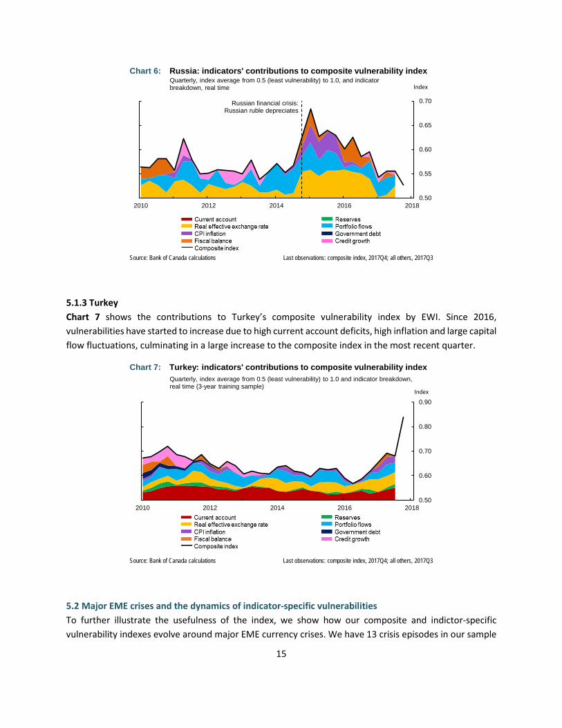
5.1.2 Russia We examine economic vulnerabilities in Russia for our second country case study. Chart 6 shows the breakdown of Russia’s composite vulnerability index by EWI. Russia experienced a spike in economic vulnerability around its financial crisis in 2014. The crisis was the result of a combination of various factors, including the oil price decline and economic sanctions due to military hostilities with Ukraine. Large capital outflows occurred in the year before the crisis, and the Russian currency depreciated rapidly beginning in 2014Q4, losing more than half of its value against the US dollar over the next 18 months. Russia’s composite vulnerability index peaked in 2015 as inflation reached double-digit figures and the government posted large fiscal deficits following the crisis. However, since then, vulnerabilities have declined to pre-crisis levels as the economy adjusted to the exchange rate and inflation came under control, although volatile portfolio investment flows remain present.
25 For the analysis in this paper, the most recent index value is estimated based on indicator data available as of March 12, 2018. Please note that we do not have all the indicator-specific data for the last observation, i.e., 2017Q4, and, therefore, the composite index value for 2017Q4 is an estimate based on partial data.
0.50
0.55
0.60
0.65
0.70
0.75
0.80
2010 2012 2014 2016 2018
Index
Brazil: indicators' contributions to composite vulnerability indexQuarterly, index average from 0.5 (least vulnerability) to 1.0 and indicator breakdown, real time
Last observations: composite index, 2017Q4; all others, 2017Q3Source: Bank of Canada calculations
Chart 5:
Political crisis: Brazilian President Rousseff impeached
15
5.1.3 Turkey Chart 7 shows the contributions to Turkey’s composite vulnerability index by EWI. Since 2016, vulnerabilities have started to increase due to high current account deficits, high inflation and large capital flow fluctuations, culminating in a large increase to the composite index in the most recent quarter.
5.2 Major EME crises and the dynamics of indicator-specific vulnerabilities To further illustrate the usefulness of the index, we show how our composite and indictor-specific vulnerability indexes evolve around major EME currency crises. We have 13 crisis episodes in our sample
0.50
0.55
0.60
0.65
0.70
2010 2012 2014 2016 2018
Index
Russia: indicators' contributions to composite vulnerability indexQuarterly, index average from 0.5 (least vulnerability) to 1.0, and indicator breakdown, real time
Last observations: composite index, 2017Q4; all others, 2017Q3Source: Bank of Canada calculations
Russian financial crisis: Russian ruble depreciates
Chart 6:
0.50
0.60
0.70
0.80
0.90
2010 2012 2014 2016 2018
Index
Turkey: indicators' contributions to composite vulnerability indexQuarterly, index average from 0.5 (least vulnerability) to 1.0 and indicator breakdown, real time (3-year training sample)
Last observations: composite index, 2017Q4; all others, 2017Q3Source: Bank of Canada calculations
Chart 7:
16
that are taken from Laeven and Valencia (2012).26 Since the crisis dates are available only at annual frequency, we convert the vulnerability indexes to annual frequency for this analysis by taking the maximum index value in each year.27
Chart 8 uses radar charts to show how EME vulnerabilities evolved around major EME crises. Each vertex of the chart represents a currency crisis. The blue, orange and red lines show the vulnerability index values two years before the crisis, one year before the crisis and during the year of the crisis, respectively; the more outward the line, the higher the index value and thus the higher the vulnerability. Looking at the composite index, vulnerabilities seem to be elevated before currency crises. This result is even more apparent when the alternative composite measure is used, as shown in Appendix 3, since the alternative composite index is based on the maximums rather than averages of the EWI-specific vulnerability indexes.
By breaking the index down into its eight subcomponents, we can get a clearer picture of the relative importance of each indicator. Elevated levels of vulnerabilities associated with the external sector, such as the current account, portfolio flows and exchange rate misalignment, generally precede the crises in our sample. Moreover, vulnerabilities related to exchange rate misalignment and portfolio flows remain high during the year of the crisis as depreciation pressures and capital flight intensify.
Vulnerabilities related to policy/sovereign sector indicators such as government debt or the fiscal balance are not as important for the onset of a currency crisis as are the vulnerabilities related to the external sector. However, high fiscal deficits preceded the currency crises in Brazil in 1999, Russia in 1998 and Ukraine in 1998. Generally, policy/sovereign sector vulnerabilities seem to increase during the year of the crisis, likely reflecting the government dealing with the consequences of the crisis. Further, vulnerabilities related to high credit growth are high in the years before the currency crises in Turkey in 2001, Russia in 1998, Malaysia in 1998 and Mexico in 1993. Nevertheless, those vulnerabilities do not seem to play a role in other currency crises.
In sum, in line with the case studies in the previous section, different historical crises are generally reflected by different vulnerabilities in terms of their composition, timing and responses. However, currency crises are generally preceded by a buildup of imbalances in the external sector followed by an increase of sovereign debt imbalances.
26 Some indicator-specific radar charts do not show certain crises because data for the given country around those crises were not available. 27 Results are largely unchanged when we use the yearly average of the quarterly index values.

17
Argentina2002
Turkey2001
Ukraine1998
Ukraine2009
Nigeria1997
Mexico1995Malaysia
1998Brazil1999
Romania1996
Philippines1998
South Korea1998
Russia1998
Thailand1998
a. Composite vulnerability index
Argentina2002
Turkey2001
Ukraine2009
Mexico1995
Brazil1999
Philippines1998
South Korea1998
Russia1998
Thailand1998
b. Current account
Argentina2002
Turkey2001
Ukraine2009
Mexico1995
Malaysia1998
Brazil1999
Romania1996
Philippines1998
South Korea1998
Russia1998
Thailand1998
c. Reserves
Argentina2002
Turkey2001
Ukraine2009
Nigeria1997
Mexico1995
Malaysia1998
Brazil1999
Philippines1998
d. Real effective exchange rate
Argentina2002
Turkey2001
Ukraine2009
Mexico1995
Brazil1999
Philippines1998
South Korea1998
Russia1998
Thailand1998
e. Portfolio flows
Argentina2002
Turkey2001
Ukraine1998
Ukraine2009
Nigeria1997
Mexico1995
Malaysia1998
Brazil1999
Romania1996
Philippines
1998
SouthKorea1998
Russia1998
Thailand1998
f. Inflation
Argentina
2002
Turkey2001
Ukraine
2009
Mexico1995
Malaysia
1998
Philippines
1998
Thailand
1998
g. Government debtRoman
ia1996
Ukraine
1998
Ukraine
2009
Mexico1995
Malaysia
1998
Brazil1999
Philippines
1998
Russia1998
Thailand
1998
h. Fiscal balanceArgentin
a2002
Turkey2001
Mexico1995
Malaysia1998
Brazil1999
SouthKorea1998
Russia1998
Thailand1998
i. Credit growth
Chart 8: Vulnerability index values prior to major EME currency crises Country-specific index, annual maximum values, scale from 0.5 to 1.0 (outward = higher level of vulnerability)
Source: Bank of Canada calculations
____ 2-year lag
____ 1-year lag ____ Contemporaneous

18
5.3 Mapping the heat in emerging-market economies Recent levels of EME vulnerability based on our approach can be easily summarized and visualized in a heat map. Table 1 shows a snapshot of the vulnerability index results across countries and EWIs for the most recent quarter of available data. Vulnerability index values are colour-coded in increments of 0.1, with green reflecting the lowest level of vulnerability and red reflecting maximum vulnerability.
Vulnerability levels can be directly compared across countries, allowing us to order them from most to least vulnerable according to their composite indexes. Currently, Egypt, Argentina, Turkey and Ukraine have the highest levels of vulnerability, while Russia, Thailand, Taiwan and South Korea show minimal signs of economic vulnerability. The heat map also shows the alternative composite index for each country; these values are higher than the baseline composite, but the rankings are similar.
0.50-0.59 0.60-0.69 0.70-0.79 0.80-0.89 0.90-1.00
FinancialComposite
indexAlternative composite
Current account
Reserves REERPortfolio inflows
InflationGov't debt
Fiscal balance
Credit growth
Egypt 0.95 1.00** 0.83** 0.56* 0.96 1.00** 0.88 - 1.00 -Turkey 0.84 0.84 0.91* 0.62* 0.92 0.81* 0.76 0.50* 0.50* 0.50*Argentina 0.83 0.89* 0.90* 0.79* 0.77 0.85* 0.88 0.70** 0.67* 0.86*Ukraine 0.75 0.85* 0.83* 0.51* 0.72 0.79* 0.79 0.87* - -Nigeria 0.72 0.83 0.50* 0.75* 0.84 - 0.82 0.50* 0.52 -Hungary 0.69 0.80 0.50* 0.50 0.55 0.63* 0.50 0.93 0.97 0.50*Colombia 0.66 0.82 0.66* 0.50 0.96 0.59* 0.50 0.67* 0.67 0.50*India 0.64 0.79 0.50* 0.50 0.76 0.54* 0.50 0.71* 0.82 0.50*Mexico 0.64 0.82 0.56* 0.52 0.87 0.79* 0.52 0.51 0.77 0.61*Malaysia 0.64 0.78 - 0.50 0.76 - 0.50 0.79 0.59* 0.50*Brazil 0.64 0.81 0.50 0.50 0.50 0.73 0.50 0.83 0.88 0.50*Romania 0.63 0.70 0.68* 0.50 0.70 0.54* 0.50** 0.50* 0.70 -South Africa 0.63 0.88* 0.63* 0.53 0.56 0.93* 0.50 0.83 0.74 0.52*Poland 0.59 0.68 0.50* 0.50 0.53 0.53* 0.50 0.71* 0.83 0.52*Costa Rica 0.59 0.59 0.55* 0.60* 0.68 0.58* 0.50 - - -Peru 0.57 0.61 - 0.50* 0.68 - 0.50 - 0.54 -Philippines 0.57 0.65* 0.50* 0.50 0.73 0.74* 0.50 0.56 0.55 -Paraguay 0.55 0.55 0.50* 0.50* 0.59 - 0.50 - 0.50* -Chile 0.54 0.68* 0.50* 0.54* 0.58 0.68* 0.50 - 0.69* 0.50*South Korea 0.54 0.76* 0.50* 0.50* 0.58 0.86* 0.50 0.67* 0.50* 0.50*Indonesia 0.53 0.70* 0.52* 0.60 0.52 0.68* 0.50 0.50 0.71* 0.50*Russia 0.53 0.62* 0.50* 0.50 0.64 0.67* 0.50 0.50 0.50 0.56*Croatia 0.52 0.98** 0.50** 0.50 0.55 0.99** 0.50 0.97* 0.50* -Taiwan 0.52 0.57 0.50 0.50 0.64 0.52 0.50 0.50 0.50 -Bulgaria 0.51 0.65** 0.50** 0.50 0.55 0.81** 0.50 0.50 - -Thailand 0.51 0.53** 0.50** 0.50 0.55 0.55** 0.50 0.50 - 0.50*
d l d i di ib i b d h li i f l i i di i h i hi i l i l di ib i d l d i
Table 1: EME vulnerability indexes by country by indicator: 2017Q2-2017Q4
Index from 0.5 to 1.0, quarterly estimates, higher index value indicates greater vulnerability1
Legend
External sector vulnerabilities Policy space vulnerabilities
1. Index values are constructed using a distribution-based measure that compares realizations of an early warning indicator with its historical cross-sectional distribution. Index values do not give the actual value of the indicator. Last observations: 2017Q4 unless otherwise indicated; *2017Q3; **2017Q2 Source: Bank of Canada calculations

19
• As of 2017Q4, our index finds Egypt was the most vulnerable EME in our sample. Its EWI-specific vulnerability indexes take on extremely high values across external and policy sector indicators, reflecting large trade and government deficits. In mid-2017, Egypt adopted an IMF-backed loan program to stabilize its economy. The immediate inflow of IMF funding accounts for Egypt’s current low level of foreign reserve vulnerability. In previous quarters, this index had been as high as Egypt’s other EWI-specific vulnerabilities. However, the IMF loan program also required Egypt to devalue and float its currency. While this should help to rectify external imbalances and support trade and economic growth in the long run, it likely further contributes to current heightened vulnerability in inflation and real exchange rate misalignment.
• In Turkey, vulnerability is heightened in the external sector through large current account deficits and portfolio inflows as well as significant real exchange rate misalignment. These external imbalances have also contributed to vulnerability in Turkey’s policy space, mostly through high inflation.
• In Argentina, vulnerabilities are elevated across almost all EWIs. Although Argentina lifted long-standing currency controls and implemented liberal economic reforms in 2015, external imbalances nonetheless remain. Additionally, although public debt has decreased from extreme levels in recent years, the corresponding vulnerability index remains high and persistent fiscal deficits remain. Argentina’s EWI-specific vulnerability indexes reflect unsustainably large portfolio investment inflows and rapid private credit growth over the end of 2016 and first half of 2017.
• In Ukraine, large vulnerabilities are related to government debt accumulated since 2014 and high inflation. These vulnerabilities partially reflect Ukraine’s hostilities with Russia and the ongoing political crisis.
In contrast, the heat map shows that Thailand and Taiwan were the least vulnerable countries over recent periods. Most notably, these countries maintain healthy current account balances and low inflation relative to other EMEs. In addition, Mexico’s vulnerabilities are relatively small or moderate except for its real exchange rate. Russia also has low overall levels of vulnerability as it successfully emerges from a long economic crisis, although portfolio outflows in 2017 may be cause for concern going forward.
5.4 Comparing current vulnerabilities to other EME risk indicators Based on the qualitative observations, we believe that Table 1 accurately reflects current vulnerabilities in EMEs. As a robustness check, we compare recent values of each country’s vulnerability indexes with Bloomberg median estimates of the probability that the country will enter a recession in the next year, taking the simple correlation between the two indexes. We use the probability of a future recession as a comparison indicator because it is a sufficiently broad measure to be comparable with all our EWI-specific vulnerability indexes, unlike alternative indicators of vulnerability such as the BIS credit gap.
We then conduct a second comparison of the vulnerability indexes with JP Morgan’s Emerging Markets Bond Index (EMBI) sovereign spreads for each country. The sovereign spreads measure the difference between the yields of US-dollar-denominated large sovereign bonds in EMEs and US Treasury yields,

20
adjusted for varying maturities. EME bond yields tend to be higher due to risk premiums; as such, the EMBI sovereign spreads can also be considered a measure of risk or economic vulnerability in EMEs.
Note that we are merely examining the crude correlation between the variables to corroborate our results; we are not testing their predictive power or for causality. Nonetheless, a positive correlation between our vulnerability indexes and either the estimated probability of entering a recession in the next year or the EMBI sovereign spread may indicate that our results are in line with external consensus views.
Chart 9 and Table 2 show the outcomes of our first robustness check. In our sample, our composite country vulnerability indexes are moderately positively correlated with probability of recession, with a correlation coefficient of 0.41. In terms of EWI-specific vulnerability indexes, our portfolio liability flows, real exchange rate and foreign reserve indexes are the most highly correlated with probability of recession.
Table 2: Vulnerability indexes and probability of recession: cross-sectional correlations External sector Policy sector Financial sector
Current account 0.24 Inflation 0.47 Credit growth 0.23 Reserves 0.38 Government debt -0.26 REER 0.42 Fiscal balance -0.15 Portfolio inflows 0.46
Composite index 0.41 Alternative composite 0.37
Source: Bloomberg and Bank of Canada estimates. Last observation: 2017Q4
Chart 10 and Table 3 show the correlations between our vulnerability indexes and the EMBI sovereign spreads in the most recent period. The correlations are generally higher here than in the probability of recession indicator; the composite index has a coefficient of 0.72. The portfolio inflows, inflation and
0.5
0.6
0.7
0.8
0.9
1.0
0
5
10
15
20
25
30
35
Egyp
t
Turk
ey
Arge
ntin
a
Ukr
aine
Nig
eria
Col
ombi
a
Indi
a
Mex
ico
Mal
aysi
a
Braz
il
Rom
ania
Sout
h Af
rica
Pola
nd
Philip
pine
s
Sout
h Ko
rea
Indo
nesi
a
Rus
sia
Taiw
an
Thai
land
Index%
Composite index Probability of recession (LHS)
Chart 9: Recent vulnerabilities in EMEs and probability of recessionAverage probability of entering recession from 2016Q4-2017Q2, Bloomberg median estimates; most recent composite vulnerability index values
Last observation: 2017Q4 Sources: Bloomberg and Bank of Canada calculations
(right scale) (left scale)

21
current account vulnerability indexes also appear to be relatively strongly correlated with sovereign spreads.
Table 3: Vulnerability indexes and sovereign bond spreads: cross-sectional correlations External sector Policy sector Financial sector
Current account 0.67 Inflation 0.86 Credit growth 0.61 Reserves 0.57 Government debt 0.01 REER 0.44 Fiscal balance -0.03 Portfolio inflows 0.79
Composite index 0.72 Alternative composite 0.72
Sources: J.P. Morgan via Haver Analytics and Bank of Canada estimates. Last observation: 2017Q4
Overall, we believe that the correlations between our vulnerability indexes and external measures of risk or vulnerability, including Bloomberg’s probability of recession indicator and the EMBI sovereign spreads, support our more qualitative assessment that our vulnerability indexes accurately reflect current economic vulnerabilities in EMEs.
6. Conclusion This paper introduces a new tool to monitor emerging-market economic and financial vulnerabilities. We obtain vulnerability indexes for several early warning indicators covering 26 EMEs. These indexes can be easily aggregated to obtain country-specific, regional or overall EME vulnerability indexes.
0.5
0.6
0.7
0.8
0.9
1.0
0
100
200
300
400
500
Egyp
t
Turk
ey
Arge
ntin
a
Ukr
aine
Nig
eria
Hun
gary
Col
ombi
a
Indi
a
Mex
ico
Mal
aysi
a
Braz
il
Rom
ania
Sout
h Af
rica
Pola
nd
Peru
Philip
pine
s
Chi
le
Indo
nesi
a
Rus
sia
IndexPercentage points
Composite index EMBI spread 2017Q4 (LHS)
Chart 10: Recent vulnerabilities in EMEs and sovereign bond spreadsMost recent composite vulnerability index values and 2017Q4 average EMBI sovereign bond spreads
Last observation: 2017Q4 Source: J.P. Morgan via Haver Analytics, Bloomberg and Bank of Canada calculations
Note: EMBI stands for the Emerging Market Bond Index by JP Morgan.
(right scale) (left scale)

22
We show visually that the emerging-market aggregate as well as regional vulnerability indexes are useful tools to assess economic vulnerabilities in real time. We demonstrate how the indexes can be used to monitor the evolution of vulnerabilities before, during and after an economic or financial crisis. Finally, we assess current EME vulnerabilities and visualize them using a heat map. Using data up to 2017Q4, we find that Egypt, Turkey, Argentina and Ukraine are currently the most vulnerable EMEs. Many of the current vulnerabilities in the most vulnerable countries stem from current account deficits, real exchange rate misalignment, volatile capital flows and high inflation.

23
References Aikman, D., M. Kiley, S. J. Lee, M. G. Palumbo and M. Warusawitharana. 2017. “Mapping Heat in the U.S. Financial System,” Journal of Banking and Finance 81 (August 2017): 36–64. Christensen, I., G. Kumar, C. Meh and L. Zorn. 2015. “Assessing Vulnerabilities in the Canadian Financial System.” Financial System Review (June): 37–46.
Frankel, J. and G. Saravelos. 2012. “Can Leading Indicators Assess Country Vulnerability? Evidence from the 2008–09 Global Financial Crisis.” Journal of International Economics 87 (2): 216–231. Laeven, L. and F. Valencia. 2012. “Systemic Banking Crises Database: An Update.” IMF Working Papers 12/163. Lee, S. J., K. E. Posenau and V. Stebunovs. 2017. “The Anatomy of Financial Vulnerabilities and Crises.” Board of Governors of the Federal Reserve System International Finance Discussion Papers No. 1191.
Pasricha, G., T. Roberts, I. Christensen and B. Howell. 2013. “Assessing Financial System Vulnerabilities: An Early Warning Approach.” Bank of Canada Review (Autumn): 10–19.
Rossi, B. and T. Sekhposyan. 2015. “Macroeconomic Uncertainty Indices Based on Nowcast and Forecast Error Distributions.” American Economic Review 105 (5): 650–655.

24
Appendix 1: Data description and sources
Indicators of Economic Vulnerabilities Indicator Description Main data source Notes
External sector
Current account balance
Balance of payments: current account surplus (positive) or deficit (negative) as a percentage of GDP
IMF Balance of Payments GDP data are taken from national sources.
Portfolio investment liabilities
Balance of payments: financial account, portfolio investment liabilities, inflows (positive) or outflows (negative), as a percentage of GDP
IMF Balance of Payments GDP data are taken from national sources. Data are unavailable for Nigeria.
Foreign exchange reserves
Stock of international reserves, including gold, end-of-period, as a percentage of annualized GDP
IMF International Financial Statistics
GDP data are taken from national sources.
Real exchange rate misalignment
Deviation of real broad effective exchange rate from past 5-year average
IMF International Financial Statistics; BIS; JP Morgan
Data for Argentina, Peru, Hong Kong, India, Indonesia, South Korea, Taiwan, Thailand and Turkey come from the BIS. Data for Egypt come from JP Morgan. All other data come from the IMF.
Policy sector
Inflation Year-over-year consumer price inflation, quarterly averages
IMF International Financial Statistics
Government debt Stock of central government debt as a percentage of annualized GDP National sources
Data are only available on an annual basis for Chile. For South Korea, Egypt and Nigeria, data are for general instead of central government debt.
Fiscal balance Fiscal surplus (positive) or deficit (negative) as a percentage of GDP National sources
Data are only available on an annual basis for Bulgaria, Ukraine, Egypt and Nigeria.
Financial sector
Private credit growth
Stock of credit to the private non-financial sector, market value, US dollars, end-of-period, year-over-year percentage change
BIS
Data are unavailable for Costa Rica, Paraguay, Peru, Philippines, Taiwan, Bulgaria, Croatia, Romania, Ukraine, Egypt and Nigeria.

25
Appendix 2: Time-varying distributions of early warning indicators
Quarterly kernel density estimates of real-time historical cross-sectional distributions
Source: Bank of Canada calculations
Current account Reserves REER
Portfolio flows Inflation Government debt
Fiscal balance Credit growth

26
Appendix 3: Alternative composite index values before major EME currency crises
Argentina2002
Turkey2001
Ukraine1998
Ukraine2009
Nigeria1997
Mexico1995
Malaysia1998
Brazil1999
Romania1996
Philippines1998
SouthKorea1998
Russia1998
Thailand1998
2-year lag 1-year lag Contemporaneous
Country-specific index, annual maximum values, scale from 0.5 to 1.0 (outward = higher level of vulnerability)
Source: Bank of Canada calculations