assessing vulnerabilities and limits in the transition to ... vulnerabilities and limits in the...
TRANSCRIPT
1
Assessing vulnerabilities and limits in the transition to renewable energies: Land requirements under 100% solar energy scenarios
Iñigo Capellán-Pérez*,a,b, Carlos de Castrob,c, Iñaki Artod
aInstitute of Marine Sciences, ICM-CSIC. Passeig Marítim de la Barceloneta, 37-49, 08003 Barcelona, Catalonia, Spain.
bResearch Group on Energy, Economy and System Dynamics, University of Valladolid, Spain.
cApplied Physics Department, Escuela de Arquitectura, Av Salamanca, 18, University of Valladolid, 47014 Valladolid,
Spain. [email protected]
dBasque Centre for Climate Change (BC3), Sede Building 1, 1st floor, Scientific Campus of the University of the
Basque Country, 48940 Leioa, Spain. [email protected]
*Corresponding author: [email protected].
Authorized Author manuscript published in “Renewable & Sustainable Energy Reviews”:
Iñigo Capellán-Pérez, Carlos de Castro & Iñaki Arto: “Assessing vulnerabilities and limits in the transition to
renewable energies: Land requirements under 100% solar energy scenarios”. Renewable & Sustainable Energy
Reviews (September 2017). https://doi.org/10.1016/j.rser.2017.03.137.
http://www.sciencedirect.com/science/article/pii/S1364032117304720
© 2017. This manuscript version is made available under the CC-BY-NC-ND 4.0 license
http://creativecommons.org/licenses/by-nc-nd/4.0/
2
Abstract
The transition to renewable energies will intensify the global competition for land. Nevertheless, most analyses to
date have concluded that land will not pose significant constraints on this transition. Here, we estimate the land-use
requirements to supply all currently consumed electricity and final energy with domestic solar energy for 40
countries considering two key issues that are usually not taken into account: (1) the need to cope with the variability
of the solar resource, and (2) the real land occupation of solar technologies. We focus on solar since it has the
highest power density and biophysical potential among renewables. The exercise performed shows that for many
advanced capitalist economies the land requirements to cover their current electricity consumption would be
substantial, the situation being especially challenging for those located in northern latitudes with high population
densities and high electricity consumption per capita. Assessing the implications in terms of land availability (i.e.,
land not already used for human activities), the list of vulnerable countries enlarges substantially (the EU-27
requiring around 50% of its available land), few advanced capitalist economies requiring low shares of the estimated
available land. Replication of the exercise to explore the land-use requirements associated with a transition to a
100% solar powered economy indicates this transition may be physically unfeasible for countries such as Japan and
most of the EU-27 member states. Their vulnerability is aggravated when accounting for the electricity and final
energy footprint, i.e., the net embodied energy in international trade. If current dynamics continue, emerging
countries such as India might reach a similar situation in the future. Overall, our results indicate that the transition to
renewable energies maintaining the current levels of energy consumption has the potential to create new
vulnerabilities and/or reinforce existing ones in terms of energy and food security and biodiversity conservation.
Key-words: Solar potential, Energy footprint, Land-use, Transition to renewable energies, Energy security.
Table of contents
1. Introduction .......................................................................................................................................................... 3
2. Materials and methods ......................................................................................................................................... 6
2.1. Multi-regional input-output model ............................................................................................................... 7
2.1.1. Electricity and final energy consumption .................................................................................................. 7
2.2. Solar power density at country level ................................................................................................. 10
2.2.1. Solar irradiance (Ii) .................................................................................................................................. 10
2.2.2. Cell efficiency conversion (f1) .................................................................................................................. 12
2.2.3. Average performance ratio over the park’s life cycle (f2) ....................................................................... 13
2.2.4. Land-occupation ratio (f3) ....................................................................................................................... 13
2.2.5. Comparison with other values estimated in the literature .................................................................... 16
2.3. Overcapacity and storage requirements due to short-term and seasonal variations ................................ 17

3
2.4. PV potential on buildings and in urban areas ............................................................................................. 21
2.5. Land-use requirements for solar power: summary .................................................................................... 23
3. Results and discussion ........................................................................................................................................ 24
3.1. 100% solar electricity mix scenario ............................................................................................................. 24
3.2. 100% solar final energy mix scenario .......................................................................................................... 28
4. Assessment of assumptions and uncertainties in estimating the land-use requirements of the transition to
RES 31
4.1. Country’s self-sufficiency in electricity/final energy and 100% solar share ............................................... 31
4.2. Static vs. dynamic projections ..................................................................................................................... 33
4.3. Estimation of solar power density at the country level .............................................................................. 34
4.4. Not accounting for EROI .............................................................................................................................. 34
4.5. PV potential in buildings ............................................................................................................................. 35
5. Conclusions ............................................................................................................................................................. 35
Acknowledgements ..................................................................................................................................................... 37
Appendix A: Electricity and final energy consumption by country for 2009 .................................................................. 37
Appendix B: CRC and SV values per country ................................................................................................................... 38
Appendix C: Potential electricity produced by rooftop PV ............................................................................................. 39
Appendix D: Share of electricity consumption covered by hydro generation ................................................................ 41
Appendix E: Total land and land per capita by scenario ................................................................................................. 41
Appendix D: Land availability at country level ................................................................................................................ 44
References .................................................................................................................................................................. 44
1. Introduction
Most governments are developing policy frameworks to promote the penetration of renewable energy sources (RES)
to improve energy security (increasingly threatened by the depletion of conventional fossil fuels) while mitigating
emissions to limit anthropogenic climate change and other negative externalities of conventional energy sources
(IPCC, 2014; Johansson, 2013; REN21, 2015; WEO, 2014). Among renewables, wind and solar are estimated to have
the greatest potential (de Castro et al., 2013; IPCC, 2011; Smil, 2010), with projections often assuming that the
resource base provides no practical limitation if adequate investments are forthcoming (e.g., IPCC (2011)).
While fossil fuels represent concentrated deposits of energy and thus can be exploited at high power rates (200-
11,000 We/m2), the technologies harnessing renewable sources are characterized by power densities several orders
of magnitude lower. Hence, for delivering the same power, RES are substantially more land intensive (Smil, 2015).
For example, typical ranges of net power density found in the literature are: 2-10 We/m2 for solar power plants, 0.5-7
We/m2 for large hydroelectric, 0.5-2 We/m2 for wind; and ~0.1 We/m2 for biomass (de Castro et al., 2014; MacKay,
4
2013; Smil, 2015). While wind farms are partially compatible with other uses (e.g., agriculture) or can be located
offshore, biomass plantations, hydroelectric reservoirs and solar farms tend not to allow double use, that is, in
practice they monopolize the occupied land. In the case of solar power, the potential in urbanized areas is limited
due to the fact that cities are currently not designed to maximize solar reception (Izquierdo et al., 2011; La Gennusa
et al., 2011; Ordóñez et al., 2010; Sorensen, 1999).
Hence, the transition to RES will add to the pressure in the global competition for land, which is already driven by
many factors (Smith et al., 2010). In particular, the dedication of land to produce energy has been identified as a
potential concern not only for preserving natural ecosystems, their services and biodiversity, but also because of its
competition with land use to cover human needs (i.e., food, fiber, shelter and infrastructure). These concerns arise in
parallel with the current rapid expansion of modern RES technologies and the steady decrease in their costs over
recent years (Deutsche Bank, 2015; REN21, 2015). Thus, this transition could aggravate existing vulnerabilities and
create new ones in terms of energy security, biodiversity loss, and food sovereignty, among others (Johansson, 2013;
MacKay, 2013; Nonhebel, 2003; Rao and Sastri, 1987; Scheidel and Sorman, 2012; Smil, 1984). As a recent example,
the occupation of just ~0.1% of Italian agricultural surface area by PV systems provoked an intense debate in the
country that ultimately lead to the ban of incentives for this technology on agricultural soil (Squatrito et al., 2014).
The relevance of the land requirements of renewables is the subject of ongoing debate, with most studies focusing
on 100% RES scenarios having estimated that the additional land requirements will not be a compelling constraint
for the transition (e.g., Jacobson and Delucchi (2011), WWF (2011), Jacobson et al., (2015), Teske et al., (Greenpeace
et al., 2015) and García-Olivares (2016)), while a few have found land availability to be a relevant biophysical
constraint that may limit the feasibility of the transition within the current socio-economic system (e.g., Mackay
(2013)). With our work, we contribute to the debate by estimating a conservative, lower bound for the land-use
requirements to supply all current consumed electricity and final energy domestically with solar energy for 40
countries, devoting special attention to uncertainties such as future efficiency improvements. We focus on solar
energy since, among renewables, it has the highest power density and biophysical potential (de Castro et al., 2013;
IPCC, 2011).
First, we concentrate on the land-use requirements and biophysical feasibility of supplying all current consumed
electricity with solar technologies in a given region as proposed by Denholm and Margolis (2008) for the states of the
USA and Šúri et al. (2007) for 30 European countries. A few estimates of solar land-use requirements have been
published to date by various authors for advanced capitalist economies such as the USA and European states
(Denholm and Margolis, 2008; MacKay, 2013; MIT, 2015; Šúri et al., 2007; Turner, 1999), and by Jacobson and
Delucchi (2011) at a global level, while other studies have focused on comparisons with other energy technologies
(Fthenakis and Kim, 2009). In general, these analyses have come up with relatively low values of solar land-use
requirements, thereby minimizing the importance of land to sustain high penetration levels of solar energy. For
example, Šuri et al. (2007) found that just 0.6% of the land surface area of the EU25 and 5 EU-candidate countries, all

5
corresponding to rooftop photovoltaic (PV), would suffice to cover the total electricity demand, with a range of 0.1-
3.6% depending on the country. Denholm and Margolis (2008) found that the land required to supply the electricity
consumed in the USA by solar plants (assuming 25% on rooftops) was between 0.3 and 0.7% of the total surface area
(with a range of 0.1-8% depending on the state). However, these analyses have not considered two key issues
included in our analysis, and these have the potential to substantially increase the land-requirements of solar power
plants:
In a 100% solar-based energy system, a substantial redundant capacity should be deployed in combination
with storage capacity to cope with the intermittence and seasonal variability of the solar resource (MacKay,
2013; Trainer, 2010, 2012, 2013a),
The real land occupation of solar technologies is five to ten times higher than the estimates usually
considered, which are based on ideal conditions (de Castro et al., 2013; MacKay, 2013; Ong et al., 2013; Smil,
2015).
Although a diversified supply combining different renewable resources as a function of their local availability would
make it possible to reduce the overcapacity and storage requirements to cope with solar intermittency to some
extent, this effect would be partially offset by the fact that for most countries solar has a power density three to five
times higher than wind, and one to two orders of magnitude higher than bioenergy and is slightly better than large
hydropower (de Castro et al., 2014; MacKay, 2013; Smil, 2015). The approach applied does not fully correspond to
an “extreme scenario” for two additional reasons: (1) there is a positive relation between the electricity
consumption per capita and income (i.e., most countries have been experiencing electrification of the energy system
for decades), and (2) the future deployment of renewables will require that this trend be intensified since they
mainly produce electricity (Armaroli and Balzani, 2011; Smil, 2008). In the period 1990 to 2007, the annual growth in
the global net electricity production (+1.9%) outpaced the annual growth in total energy consumption (+1.3%), a
trend which is expected to strengthen in the next few decades. For example, the International Energy Agency (IEA) in
its New Policies Scenario expects the world electricity demand to grow by 2.1% per year on average between 2012
and 2040 (i.e., +80% cumulative growth in the period), its share of total energy use rising in all sectors and regions
(WEO, 2014). Thus, the land occupation by solar/RES in the future is likely to be higher than estimated in our study
for current electricity consumption.
Additionally, a third factor, critical for assessing potential vulnerabilities, is considered: over recent years, advanced
capitalist countries have specialized in economic activities with high added value (reducing their share of energy
intensive sectors and manufacturing industries) while some emerging economies, like China and India, have
undergone a process of rapid industrialization, increasing their share in the global economy, and are exporting
enormous volumes of manufactured products to developed countries (Baiocchi and Minx, 2010; Weber, 2009). This
shift of economic activities between countries has also had consequences in terms of energy use. Arto et al. (2016)
showed that an increasingly large proportion of the energy used by emerging countries is being devoted to sustain
6
the welfare of advanced capitalist economies by means of international trade. Hence, together with data on the
electricity use per country, we will consider the net electricity consumption after accounting for international trade
for each country, i.e., its electricity footprint, estimated from the multi-regional input-output model (MRIO) WIOD
(Dietzenbacher et al., 2013).
In a second stage, we replicate the analysis to explore the land implications and biophysical feasibility, for each
country, of supplying all current final energy consumption by solar systems. Again, this approach must not be seen as
an extreme, e.g., the world primary energy demand is expected to increase by almost 40% by 2040 (WEO, 2014).
Thus, the exercise performed will allow us to test MacKay’s affirmation that: “…in a world that is renewable-
powered, the land area required to maintain today’s British energy consumption would have to be similar to the
area of Britain. The same goes for Germany, Japan, the Republic of Korea, Belgium and the Netherlands” (MacKay,
2013). If these numbers were to be confirmed, far from enhancing their energy security as usually claimed, the
transition to renewable energies in some countries in the current socio-economic context would instead increase
their external dependence and vulnerability (Johansson, 2013; Lilliestam and Ellenbeck, 2011; Moriarty and Honnery,
2016; Trainer, 2013b).
The paper is organized as follows: Section 2 includes the literature review related to the estimation of land
requirements for solar technologies and describes the materials and methods used, Section 3 presents the results
obtained and discusses them, Section 4 assesses the main assumptions and uncertainties considered in the analysis
and Section 5 outlines our conclusions.
2. Materials and methods
In order to assess the total land requirements of solar generation at the country level, we performed a literature
review related to estimating land requirements for solar technologies which informed the choice of methods used in
the analysis. These methods were implemented in the following steps:
Calculation of the electricity and final energy consumption by country for the year 2009 from a
terrestrial-perspective (electricity/final energy use) and a consumption-based perspective
(electricity/final energy footprint) (Section 2.1),
Estimation of a likely range for the solar power density by country considering future technological
advances (Section 2.2),
Conservative estimation of the overcapacity needed by country to deal with the intermittence and
seasonal variations in the solar resource (Section 2.3),
Estimation of the potential share of the electricity to be covered by rooftop PV on buildings by country
(Section 2.4).
Having estimated these factors, the land-use requirements per country to supply an amount of energy by solar
power can be obtained by applying the following formula:

7
Equation (1)
2.1. Multi-regional input-output model
Input-output tables display the interconnection between different sectors of production, making it possible to track
the production and consumption in an economy. Traditionally, energy consumption has been described by the
“energy use” indicator that refers to the amount of energy used within the borders of a country. However, in the last
decade, the acceleration of economic processes linked to globalization (e.g., specialization and offshoring) has
resulted in a shift of economic activities between countries and in a dramatic growth in international trade.
Advanced capitalistic economies have specialized in economic activities with high added value, while reducing their
share of energy intensive sectors and manufacturing industries (Baiocchi and Minx, 2010; Weber, 2009). In relation
to this, MRIO tables allow us to track the global supply chains of products consumed by including the trade between
different countries. In this paper, we combine the common “electricity use” (or territorial-based) indicator with the
concept of an “electricity footprint” (or consumption-based) indicator which relates to the electricity consumed
worldwide to produce the goods and services demanded by the people living in a given country.
We apply the WIOD (Dietzenbacher et al., 2013), a set of MRIO tables that comprises information for 35 industries,
59 products for the 27 member states of the European Union (EU-27), and 13 non-EU countries (Australia, Brazil,
Canada, China, India, Indonesia, Japan, South Korea, Mexico, Russia, Turkey, and the United States of America
(USA)), as well as the Rest of the World (RoW) as an aggregated region. These 40 countries represent 65% of world's
population and 90% of the GDP. Although the WIOD presents data from 1995 to 2009, here we concentrate on the
last year of the series to perform a static analysis.
The energy (electricity and final energy) use and footprint per country are obtained following the methodology
described in Arto et al. (2016). Since the proposed analysis assumes that all the electricity production is substituted
by solar power plants, we took the total final electricity consumption as well as the electric power transmission and
distribution losses from the IEA Energy Balances for the year 2009 (IEA, 2016a). Consistency is ensured by
considering own consumption by the solar power plants in the f2 factor (see Section 2.2).
2.1.1. Electricity and final energy consumption
The electricity and final energy consumption (use and footprint) calculated for the target countries in 2009 is shown
in Figure 1a and b (see Table A1). The countries are sorted in descending order according to the national means in
terms of energy use.
For countries with the highest electricity use per capita (Canada, Finland, Sweden and USA), the electricity use
ranges from 13.5 to 16.5 MWh/person/year with differences between the electricity footprint and electricity use per
capita of -13% (Sweden) to +9% (USA). At the other extreme, in the countries with the lowest electricity
8
consumption (India, Indonesia, Mexico and China), the electricity use ranges from 0.5 to 2.5 MWh/person/year, with
differences between the electricity footprint and use use of -21% (China) to +15% (Indonesia). Most European
countries are characterized by electricity footprints per capita higher than their electricity use, notably Greece
(+36%), Denmark (+35%), Ireland (+29%) and the UK (+22%), whereas countries such as Russia (-24%), China (-21%)
and South Korea (-16%) are net exporters of electricity embodied in trade (Figure 1a).
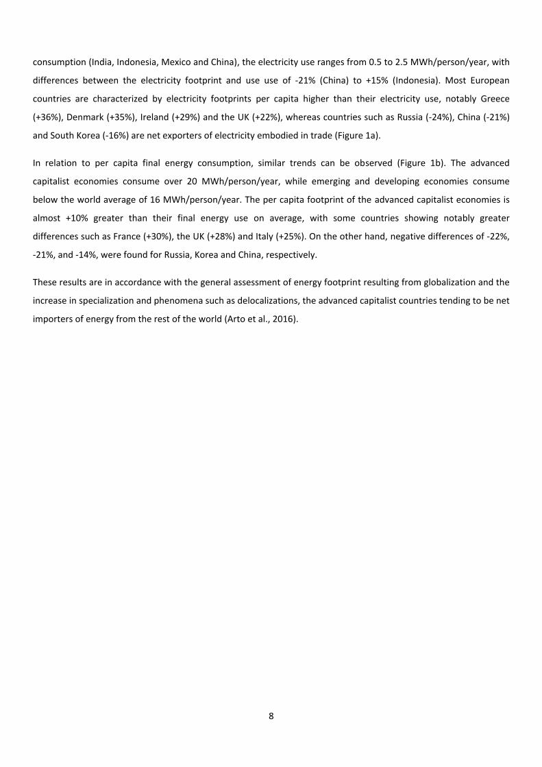
In relation to per capita final energy consumption, similar trends can be observed (Figure 1b). The advanced
capitalist economies consume over 20 MWh/person/year, while emerging and developing economies consume
below the world average of 16 MWh/person/year. The per capita footprint of the advanced capitalist economies is
almost +10% greater than their final energy use on average, with some countries showing notably greater
differences such as France (+30%), the UK (+28%) and Italy (+25%). On the other hand, negative differences of -22%,
-21%, and -14%, were found for Russia, Korea and China, respectively.
These results are in accordance with the general assessment of energy footprint resulting from globalization and the
increase in specialization and phenomena such as delocalizations, the advanced capitalist countries tending to be net
importers of energy from the rest of the world (Arto et al., 2016).

9
a
b
0
3
6
9
12
15
18C
anad
aFi
nlan
dSw
eden
Un
ited
Sta
tes
Luxe
mb
ou
rgA
ust
ralia
Taiw
anSo
uth
Ko
rea
Jap
anB
elgi
um
Fran
ceA
ust
ria
Net
her
land
sG
erm
any
Ru
ssia
Est
on
iaSl
oven
iaC
ypru
sC
zech
Rep
ubl
icIr
elan
dEU
-27
Den
mar
kSp
ain
Un
ited
Kin
gdo
mG
ree
ceIt
aly
Mal
taP
ort
uga
lSl
ova
kia
Bu
lgar
iaH
unga
ryP
olan
dLi
thu
ania
Wo
rld
Ch
ina
Turk
eyB
razi
lR
om
ania
Mex
ico
Res
t o
f th
e w
orld
Ind
iaIn
do
nes
ia
MW
h/y
ear
/pe
rso
n
Per capita electricity consumption
Electricity useElectricity footprint
World mean
0
20
40
60
80
100
120
Luxe
mb
ou
rgC
anad
aFi
nlan
dU
nit
ed S
tate
sD
enm
ark
Bel
giu
mN
eth
erla
nd
sA
ust
ralia
Swed
enT
aiw
an
Sou
th K
ore
aA
ust
ria
Ru
ssia
Ge
rma
ny
Irel
and
Jap
anC
ypru
sC
zech
Rep
ubl
icEU
-27
Fra
nce
Mal
taU
nit
ed K
ingd
om
Gre
ece
Esto
nia
Slo
ven
iaIt
aly
Spai
nSl
ovak
iaP
ortu
gal
Hun
gary
Pol
and
Latv
iaLi
thu
ania
Bu
lgar
iaM
exic
oC
hin
aT
urk
ey
Bra
zil
Ro
man
iaR
est
of
the
wor
ldIn
do
nes
iaIn
dia
MW
h/y
ear
/pe
rso
n
Per capita final energy consumption
Final energy useFinal energy footprint
World mean
10
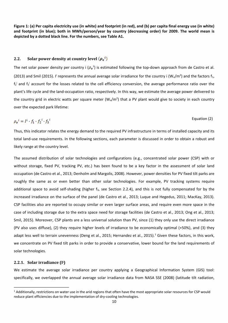
Figure 1: (a) Per capita electricity use (in white) and footprint (in red), and (b) per capita final energy use (in white) and footprint (in blue); both in MWh/person/year by country (decreasing order) for 2009. The world mean is depicted by a dotted black line. For the numbers, see Table A1.
2.2. Solar power density at country level
The net solar power density per country i ( ) is estimated following the top-down approach from de Castro et al.
(2013) and Smil (2015). Ii represents the annual average solar irradiance for the country i (We/m2) and the factors f1,
f2i and f3
i account for the losses related to the cell efficiency conversion, the average performance ratio over the
plant’s life cycle and the land-occupation ratio, respectively. In this way, we estimate the average power delivered to
the country grid in electric watts per square meter (We/m2) that a PV plant would give to society in each country
over the expected park lifetime:
Equation (2)
Thus, this indicator relates the energy demand to the required PV infrastructure in terms of installed capacity and its
total land-use requirements. In the following sections, each parameter is discussed in order to obtain a robust and
likely range at the country level.
The assumed distribution of solar technologies and configurations (e.g., concentrated solar power (CSP) with or
without storage, fixed PV, tracking PV, etc.) has been found to be a key factor in the assessment of solar land
occupation (de Castro et al., 2013; Denholm and Margolis, 2008). However, power densities for PV fixed tilt parks are
roughly the same as or even better than other solar technologies. For example, PV tracking systems require
additional space to avoid self-shading (higher f3, see Section 2.2.4), and this is not fully compensated for by the
increased irradiance on the surface of the panel (de Castro et al., 2013; Luque and Hegedus, 2011; MacKay, 2013).
CSP facilities also are reported to occupy similar or even larger surface areas, and require even more space in the
case of including storage due to the extra space need for storage facilities (de Castro et al., 2013; Ong et al., 2013;
Smil, 2015). Moreover, CSP plants are a less universal solution than PV, since (1) they only use the direct irradiance
(PV also uses diffuse), (2) they require higher levels of irradiance to be economically optimal (+50%), and (3) they
adapt less well to terrain unevenness (Deng et al., 2015; Hernandez et al., 2015).1 Given these factors, in this work,
we concentrate on PV fixed tilt parks in order to provide a conservative, lower bound for the land requirements of
solar technologies.
2.2.1. Solar irradiance (Ii)
We estimate the average solar irradiance per country applying a Geographical Information System (GIS) tool:
specifically, we overlapped the annual average solar irradiance data from NASA SSE (2008) (latitude tilt radiation,
1 Additionally, restrictions on water use in the arid regions that often have the most appropriate solar resources for CSP would reduce plant efficiencies due to the implementation of dry-cooling technologies.
11
i.e., the radiation incident on a surface positioned such that the tilt coincides with the latitude, which is the optimal
angle for PV panels to take advantage of the solar resource at each location) with the surface area of each country.
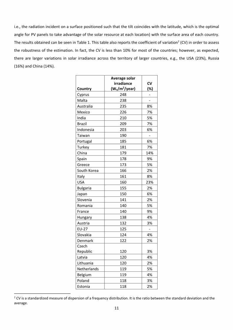
The results obtained can be seen in Table 1. This table also reports the coefficient of variation2 (CV) in order to assess
the robustness of the estimation. In fact, the CV is less than 10% for most of the countries; however, as expected,
there are larger variations in solar irradiance across the territory of larger countries, e.g., the USA (23%), Russia
(16%) and China (14%).
Country
Average solar irradiance
(We/m2/year) CV
(%)
Cyprus 248 -
Malta 238 -
Australia 235 8%
Mexico 226 7%
India 210 5%
Brazil 209 7%
Indonesia 203 6%
Taiwan 190 -
Portugal 185 6%
Turkey 181 7%
China 179 14%
Spain 178 9%
Greece 173 5%
South Korea 166 2%
Italy 161 8%
USA 160 23%
Bulgaria 155 2%
Japan 150 6%
Slovenia 141 2%
Romania 140 5%
France 140 9%
Hungary 138 4%
Austria 132 3%
EU-27 125 -
Slovakia 124 4%
Denmark 122 2%
Czech Republic 120 3%
Latvia 120 4%
Lithuania 120 2%
Netherlands 119 5%
Belgium 119 4%
Poland 118 3%
Estonia 118 2%
2 CV is a standardized measure of dispersion of a frequency distribution. It is the ratio between the standard deviation and the average.

12
Germany 118 6%
Luxembourg 117 1%
Canada 117 15%
Russia 113 16%
United Kingdom 108 7%
Ireland 104 6%
Sweden 104 10%
Finland 102 8%
Table 1: Estimates of the annual average solar irradiance and coefficient of variation (CV) for the countries in the WIOD database from (NREL, 2014). The data are surface area-weighted averaged to the different solar irradiance levels in each country. For Taiwan, Malta and Cyprus, we approximated the country irradiance using the irradiance level of its CRC due to the small size of each country (see Section 2.3). The value for the UE-27 is calculated from the area-weighted values of each country member (not from GIS calculation).
2.2.2. Cell efficiency conversion (f1)
Current average efficiencies from single and polycrystalline silicon cells are between 10 and 12% (de Castro et al.,
2013; Smil, 2015). The best current research cell efficiencies under standard test conditions (STC)3 are as follows:
8.6-17.9% for emerging techniques, 13.4-23.3% for thin films, 20.4-27.6% for crystalline silicon cells and 26.4-44.7%
for multi-junction cells (Smil, 2015). Although future technologies will improve on current efficiencies, it is unclear
whether future parks will increase average efficiencies beyond 20%. For example, thin film technologies (currently
representing roughly 10% of the share (ISE, 2014)) might lead the way in the future due to their economic advantage
(MacKay, 2013). In relation to multi-junction cells, their higher efficiency is gained at the cost of substantially greater
manufacturing complexity and price. Moreover, they are mostly installed in double tracked systems where the
greater demand for space is not compensated for by a better power density. To date, their use has been limited to
special applications, notably in aerospace where their high power-to-weight ratio is worthwhile. On the other hand,
single-junction cells have a maximum theoretical efficiency of 34%, a thermodynamic limit known as the Shockley–
Queisser limit (Luque and Hegedus, 2011).
Further, material constraints might emerge at significant solar power deployment levels (e.g., copper, silver) (de
Castro et al., 2013; García-Olivares et al., 2012). In general, the efficiency of the cells made with abundant materials
(e.g., amorphous silicon) tends to be relatively lower than those made with materials that are less abundant (e.g.,
cadmium telluride or polycrystalline silicon).
Thus, to take into account the uncertainties in future technological developments and market share, we consider 15
to 25% to be a plausible range for the future average cell efficiency conversion of installed PV capacity (de Castro et
al., 2013). At the lower limit, simpler and cheaper technologies such as thin-film or amorphous silicon would
3 PV modules are rated in laboratories at STC in watts of peak power (Wp). This is the power the module would deliver to a
perfectly matched load when the module is illuminated with 1 kW/m2 of insolation power of a certain standard spectrum
(corresponding to bright sunlight) while the cell temperature is fixed at 25ºC and air mass at 1.5 spectrum). An array of modules is
rated by summing up the watts peak of all the modules (Luque and Hegedus, 2011).

13
dominate the market, while the upper limit would reflect a situation in which the more complex and expensive
technologies were substantially deployed. This parameter is set equally for all countries since the current PV market
is global (REN21, 2015).
2.2.3. Average performance ratio over the park’s life cycle (f2)
Solar cell efficiencies are rated in laboratories under controlled conditions, which will be different from real outdoor
installations (generally, the irradiance being lower and the temperature higher). There are also losses in the wiring
and the inverter, and related to the time for maintenance, among other factors. The ratio between the actual and
the nominal output is therefore expressed by a gross measure, the performance ratio (PR). There are many PRs
defined in the scientific literature, these ranging from 0.4 to 0.8, considering different limits and conditions (de
Castro et al., 2013; Luque and Hegedus, 2011). Solar manufacturers, however, usually perform PR calculations that
do not take into account factors such as the average degradation of the photovoltaic cells over the expected plant
lifetime, electrical losses from the current meter to the connection to the electricity grid, losses due to failures of
modules or inverters, corrosion and cabling issues or energy self-consumption (other than electric) for the
maintenance of the solar park installations. Including these additional losses makes it possible to estimate the
average performance ratio over the park’s lifetime. Following this approach, de Castro et al., (2013) estimated a PR
value of 0.67. Prieto and Hall (2013) estimated this parameter performing an energy output analysis under actual
operating conditions in Spain, taking into account the future degradation of the cells but ignoring availability and
self-consumption, shading and other losses, and obtained a PR value of 0.655. Thus, in this work, we take the value
0.65 as a reference for the parameter f2. However, in warmer climates, the PR is lower because the efficiency of the
cell falls with increasing temperature. Luque and Hegedus (2011) report a 5–10% reduction when the ratings are
made at 45°C instead of under STC (i.e., 25°C), and hence, we apply a 7.5% reduction for the countries analyzed that
lie within the tropics.
2.2.4. Land-occupation ratio (f3)
The land-occupation ratio is the actual land occupation of PV cells over the total land occupation of solar
photovoltaic power plants. This includes the space required around the modules to avoid shading, for substations to
allow for maintenance including access roads, service buildings, etc., i.e., all land enclosed by the site boundary.
Near-field shading considers local obstructions, such as trees, walls, rooftop equipment, and neighboring rows
of panels, and can have a substantial impact on PV output.4 This factor cannot be explicitly taken into account in this
work due to the top-down approach applied; however, it is already implicitly included in our estimation of f3 (see, for
example, the Lieberose park surface area occupation in Figure 2 in de Castro et al., (2013)). For multi-row
commercial systems, row-to-row shading is inevitable, but designers have the ability to choose array geometry to
4 Near-field shading is electrically equivalent to mismatch. If one module in a string is shaded it may have the same effect as if the
entire string were shaded, as the entire string can only carry the same amount of current as its weakest link. Shade on as little as 5–
10% of an array can be predicted to reduce its output by over 80% (Luque and Hegedus, 2011).
14
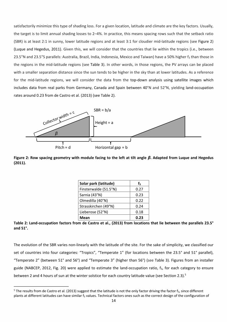
satisfactorily minimize this type of shading loss. For a given location, latitude and climate are the key factors. Usually,
the target is to limit annual shading losses to 2–4%. In practice, this means spacing rows such that the setback ratio
(SBR) is at least 2:1 in sunny, lower latitude regions and at least 3:1 for cloudier mid-latitude regions (see Figure 2)
(Luque and Hegedus, 2011). Given this, we will consider that the countries that lie within the tropics (i.e., between
23.5°N and 23.5°S parallels: Australia, Brazil, India, Indonesia, Mexico and Taiwan) have a 50% higher f3 than those in
the regions in the mid-latitude regions (see Table 3). In other words, in those regions, the PV arrays can be placed
with a smaller separation distance since the sun tends to be higher in the sky than at lower latitudes. As a reference
for the mid-latitude regions, we will consider the data from the top-down analysis using satellite images which
includes data from real parks from Germany, Canada and Spain between 40°N and 52°N, yielding land-occupation
rates around 0.23 from de Castro et al. (2013) (see Table 2).
β
Pitch = d
Height = a
Horizontal gap = b
SBR = b/a
Figure 2: Row spacing geometry with module facing to the left at tilt angle β. Adapted from Luque and Hegedus (2011).
Solar park (latitude) f3
Finsterwalde (51.5°N) 0.27
Sarnia (43°N) 0.23
Olmedilla (40°N) 0.22
Strasskirchen (49°N) 0.24
Lieberose (52°N) 0.18
Mean 0.23
Table 2: Land-occupation factors from de Castro et al., (2013) from locations that lie between the parallels 23.5° and 51°.
The evolution of the SBR varies non-linearly with the latitude of the site. For the sake of simplicity, we classified our
set of countries into four categories: “Tropics”, “Temperate 1” (for locations between the 23.5° and 51° parallel),
“Temperate 2” (between 51° and 56°) and “Temperate 3” (higher than 56°) (see Table 3). Figures from an installer
guide (NABCEP, 2012, Fig. 20) were applied to estimate the land-occupation ratio, f3, for each category to ensure
between 2 and 4 hours of sun at the winter solstice for each country latitude value (see Section 2.3).5
5 The results from de Castro et al. (2013) suggest that the latitude is not the only factor driving the factor f3, since different plants at different latitudes can have similar f3 values. Technical factors ones such as the correct design of the configuration of

15
Geographical region
SBR f3
Tropics < 23.5° 2:1 0.34
Temperate1 23.5° < x < 51° 3:1 0.23
Temperate2 51° < x < 56° 4:1 0.17
Temperate3 > 56° 6:1 0.11
Table 3: Four categories of geographical regions that represent the f3 associated with the setback ratio (SBR) that avoids shading at the winter solstice between 2 and 4 hours. Source: (NABCEP, 2012). f3 from the geographical region Temperate 1 as the reference.
Table 4 summarizes the estimates of the likely ranges of the parameters f1, f2 and f3, and Figure 3 shows the
estimated range of solar power density by WIOD country applying Equation (2). The whole range is 1.1-12.1
We/m2/year (Figure 3). The spread is significant for all regions, due to the uncertainty in the efficiency conversion
from solar irradiance arriving at the panel to the cell (f1 between 0.15 and 0.25, 66% difference). Among the
countries with the highest power density values, those in the tropics such as Australia, Mexico, India, Brazil and
Indonesia have notably high values of between 8.4 ± 2.1 and 9.7 ± 2.4 We/m2/year. However, most countries are
characterized by more modest values of 3 to 8 We/m2/year. Finally, the lowest values are found for regions that are
located in parallels even further from the equator, such as Russia, Poland, Denmark, Netherlands, the UK and Ireland
(2-4 We/m2/year ) and the Baltic states and Nordic countries (< 3 We/m2/year).
Loss
factor
Units Description Future range estimate
f1 Ad Efficiency conversion from solar irradiance
arriving at the panel to the cell
0.15-0.25
(current estimate: 0.12)
f2 Ad Average performance ratio over the park’s life
cycle including degradation, losses, failures, etc.
Tropics 0.60
Rest 0.65
f3 Ad Land-occupation ratio Tropics 0.34
Temperate 1 0.23
Temperate 2 0.17
Temperate 3 0.11
Table 4: Estimates of the current and likely future values of the loss factors fi. See discussion of the estimates in Section 2.2. The countries within the tropics are: Australia, Brazil, India, Indonesia, Mexico and Taiwan.
the infrastructure in the field (and sometimes the shape of the field itself (see, for example, the Olmedilla plant in de Castro et al. (2013, Fig. 6)) are found to be critical to maximize the solar power density of each plant.

16
Figure 3: Estimated average solar power density per country (We/m2/year) considering uncertainty in the efficiency of future PV modules and specific geographical characteristics.
2.2.5. Comparison with other values estimated in the literature
Few studies have provided power density estimates of solar technologies that analyze real power plants. Smil (2015)
reviewed the largest PV projects in operation, finding a range of 3-9 We/m2/year depending on the technology and
geographical location of the site. De Castro et al. (2013) and Ong et al. (2013) highlighted the importance of
assessing the entire land occupation of solar parks through the analysis of satellite images to identify plant
configuration, direct land use and project area boundaries, since official project data are often unavailable or do not
reflect the actual occupation of the infrastructure. Ong et al. (2013) analyzed 72% of installed and under-
construction utility-scale PV and CSP capacity in the USA, finding a generation-weighted average of the total land-use
requirements6 of 6.9 We/m2/year for small PV, 8.3 We/m2/year for large PV and 8.1 We/m2/year for CSP. These values
are lower than those applied by Denholm and Margolis (2008), who took a PV ground-based array power density
value for fixed panels which translated to a ~30% overestimation of the power density. Our estimated average
power density for the USA is in the range of 3.6-6 We/m2/year, which is even lower than that found by Ong et al.
(2013). This difference can be explained by several factors, in particular, the fact that they used a higher PR derived
from solar manufacturers, and the fact that most of the current parks are installed in areas with very high irradiance
levels (i.e., exceeding 250 We/m2/year, in California and Arizona; see also the CV obtained for the USA in Table 1). On
6 The total estimated area corresponds to all land enclosed by the site boundary, and the direct area comprises land directly
occupied by solar arrays, access roads, substations, service buildings, and other infrastructure.

17
the other hand, only 15% of the projects analyzed by Ong et al. (2013) refer to completed projects; and hence, they
relied to a large extent on manufacturers’ data, which have been shown to systematically overestimate the power
density of the real parks (de Castro et al., 2013).7
In terms of land use energy intensity (the inverse of ρe), our equivalent range is 9.4-99.8 m2yr/MWh. Specifically, the
values for all countries, except for the Scandinavian and Baltic countries (Finland, Sweden, Estonia, and Latvia), lie
within the range found in a literature review (Horner and Clark, 2013). However, this review only included one study
at typical Scandinavian solar irradiance (see ref [5] in Horner and Clark (2013)) without taking into account the
additional shadowing in these latitudes (f3=0.33).
2.3. Overcapacity and storage requirements due to short-term and seasonal variations
For each location, the solar resource is variable over time, with both short-term variability (e.g., cloudiness, day-
night) and seasonal variability (e.g., winter-summer), the latter completely uncorrelated with the demand. Usually, a
grid can accommodate up to only 20% electricity from renewable sources without a need for dedicated storage
facilities (Armaroli and Balzani, 2011; Lenzen, 2010). Thus, with the hypothesis that all the national electricity would
be produced by solar power, a certain level of (1) storage, (2) overcapacity and (3) flexible demand should then be
considered. In this work, we focus on the two first elements, distinguishing between short-term and seasonal
variability.
For the short-term variability, we focus on hydro pumping storage as proposed by other authors (Denholm and
Margolis, 2008). Although electric batteries might also address the short-term variability,8 hydroelectric pumping
storage is currently the best solution due to its demonstrated functioning, competitive cost, high efficiency, long
storage times (up to years) and fast response (Armaroli and Balzani, 2011). This solution would require the
construction of a certain amount of additional capacity to compensate for the related losses, which for pumped
storage are typically of the order of 25% (χ factor in Equation (8), i.e., a round-trip storage efficiency of 75%)
(Denholm and Kulcinski, 2004; Denholm and Margolis, 2008; MacKay, 2013). These losses apply only to the fraction
of demand passing through storage (fstor). The estimation of this fraction should ideally be done at the country level
comparing hourly load to hourly PV supply (e.g., (Wagner, 2014)), which is far beyond the scope of this paper.
Instead, as a reference value, we used the middle of the range (60-70%) found by Denholm and Margolis (2008) for a
variety of regions in the USA. This approach based on hydro pumping is simplistic and conservative since it may be
impossible to achieve the required storage volumes depending on the population density and the climate and
geography of the country (Trainer, 2012). For example, MacKay (2013) estimated that summer/winter balancing for
the UK would require lakes for pumped storage occupying 5% of the area of the country, which is physically
unfeasible. Trainer (2013a) estimated for Europe that generation from pumped storage would have to be scaled up
7 The report also lacks of information to assess differences in the estimation of the f3 parameter. For example, the only table that
would allow for a comparison (Table 5), reports only seven parks with a power density of 4-6.7 We/m2/year, which are all values
lower than the reported average (8.3 We/m2/year). 8 In particular, electric cars may act as storage devices. The IEA (2016b) estimates that “125,000 cars could be equivalent to 300
MW of flexibility – a medium size pump storage plant or a successful stationary demand side response program”.

18
by a factor approaching 20.9 CSP with storage could also help to mitigate the short-term variability, though unlike
hydro it would not be a universal solution, since it requires high irradiance locations with low cloudiness to operate
at profitable rates (typically desert areas). Additionally, CSP has a higher seasonal variability than PV. For instance, in
Spain, the ratio of the highest/lowest monthly production is 9 for all CSP installations but 2.6 for the PV facilities
(REE, 2016).
In relation to seasonal variability, depending on latitude (e.g., winter-summer) and the regional climate
characteristics (cloud cover, monsoon, etc.), there may be substantial differences in average monthly irradiance
levels (Smil, 2015; Trainer, 2012). For example, although the minimum average monthly irradiance level represents
over 90% of the annual average for cities such as Jakarta (Indonesia) or Rio de Janeiro (Brazil), in other cities such as
London (UK), Paris (France) and Berlin (Germany), this ratio falls below 40% (NASA SSE, 2008). These differences are
reflected in actual PV electricity generation: for example, in 2014, the electricity from solar in Germany was over 5
TWh in June and just 0.4 TWh in December, an order of magnitude difference.10 This difference cannot be exclusively
attributed to the difference in monthly irradiance since the minimum is only around 30% lower than the maximum
(see Table B1), and is likely related to the increased shadowing in winter (especially critical on rooftops, see Section
2.4). Thus, previous studies considering only average annual irradiance levels without including the seasonal
variability when estimating the solar potential of different countries and states (e.g., (Denholm and Margolis, 2008;
Šúri et al., 2007)), underestimate the actual capacity (and land-use requirements) required to produce the electricity
in months in which the irradiance is substantially lower than the annual average (Trainer, 2012, 2010).
Apart from hydro pumping storage systems to compensate for the seasonal variations are not yet available and
alternative technologies of large-scale storage are still in the R&D phase (Wagner, 2014). Thus, here we propose a
novel approach to produce a conservative estimate of the additional capacity required to take into account seasonal
variations at different geographical locations. We posit that, for each country, the total installed capacity should be
able to cover the electricity consumption in the month with the lowest solar irradiance level.11 This process consists
of the following steps:
a) Since within a given country (and especially those with large surface areas), there may be locations with very
different solar irradiance potentials, we start by estimating a reference geographical coordinate center (the
country-specific “central reference coordinate”, CRCi) with longitude CRClgi and latitude CRClat
i.
b) CRClati was taken at approximately12 +1/3 of the distance between the minimum and the maximum longitude
relative to the country i, from its closest area to the equator. For example, the latitude in the case of Spain
9 However, the identified total technical potential for hydropower in Europe only doubles current installed capacity (IPCC, 2011). 10 http://www.solarwirtschaft.de/en/photovoltaic-market.html 11 In most countries, the winter consumption of electricity is higher than in summer (excepting those in tropical regions with a
substantial use of air conditioning). Thus, the approach is internally consistent since by assigning a monthly annual average to
winter, we are in fact underestimating the actual demand of electricity. 12 For some countries with very low irradiance and an elongated geographical shape such as Finland and Sweden the +1/3 criteria
was softened to move the CRC to the south.

19
ranges between 36°N and 44°N and thus its CRClat would then be 36+(44-36)*1/3 ~ 39°N. The reason to take
1/3 instead of, for example, ½, was to consider that locations with better solar resources are more
economically attractive and will tend to be occupied first (as is occurring for CSP plants in the USA (Ong et
al., 2013), for example, although there are exceptions such as Australia where the majority of plants are
close to the largest cities in the south of the country).
c) CRClgi: starting from CRClat
i, we take the longitude values encompassed by the country. From this set of
values, we select the longitude with the smallest difference between the value in the month with the lowest
irradiance and the annual value, i.e., the most favorable longitude given the latitude. For example, Spain is
characterized by the latitude 39°N and spans the longitude values 0, 1, 2, 3, 4, 5, 6 and 7°W (large variations
can exist: for example, for Luxembourg there was only one longitude value while for Russia there were 90).
The longitude level with the smallest difference between the value in the month with the lowest irradiance
and the annual average was 0°W (thus, the CRC for Spain is 39°N 0°W). We call this ratio the seasonal
variability (SV) and in the case of Spain it is estimated to be 0.7 (see Table B1).13 Minor adjustments were
made to ensure that the CRC annual average irradiance is greater than the country average (compare with
Table 1).
Hence, the overcapacity factor per country i to deal with short-term and seasonal variations can be expressed as (see
the country values in Table B1):
Equation (3)
These overcapacity requirements can be as low as +30% (Australia) or 3 to 5-fold for those countries with a lower SV
(typically northern European countries). In fact, as shown by Weitemeyer et al. (2015) with an hourly resolution
study for Germany, while a 50-80% share of intermittent renewable sources may require relatively low levels of
storage and overcapacity, a system 100% based on intermittent sources substantially increases these requirements,
i.e., there is an asymptote when approaching the full intermittent energy mix. Our result for Germany (2.8-fold
overcapacity) is in good agreement with their range.14
Figure 4 illustrates the seasonal and geographical variations in the solar irradiance at the CRC for five representative
countries. The CRC for the UK represents a typical northern European country characterized by a low irradiance and
13 The following case illustrates the conservative nature of the estimated SV in this analysis. In Spain, the PV electricity
production in 2014 in two months (January and November) was less than 60% of the annual average of PV electricity production.
In 2015, December was the worst case for PV generation. Considering other renewables in December 2015, wind electricity
production was 88% of the annual average, hydroelectricity was 61% of its annual average and CSP only 20% of its annual
average. Therefore, even an ideal renewable mix will likely require overcapacity/storage for some months, and our SV is likely
optimistic (own calculations based on (REE, 2016)). 14 In fact, their study: (1) assumes no grid limitations, and (2) considers seasonal storage capacities and technologies (such as
hydrogen) that are currently not commercially available on a gigantic scale. In their own words: “… the results derived from our
approach for large-scale systems […] exhibit lower bounds for the actual storage demand” (Weitemeyer et al., 2015).

20
large seasonal variations (with winter values below 50% of the annual average, while reaching almost 150% in
summer). The CRC for Greece is typical of that for Mediterranean countries, where significantly high irradiance
values are reached during most of the year although still with a substantial seasonal variability. The Indonesian CRC
represents a country with a high and stable solar irradiance over the year, while that for Australia shows an area
with very high and stable solar irradiance. The influence of the monsoon is visible in the Indian CRC, provoking a
decrease in the summer months from over 250 We/m2 to below 200 We/m2.
0
50
100
150
200
250
300
Jan Feb Mar Apr May Jun Jul Aug Sep Oct Nov Dec
We
/m²/
year
CRC latitude tilt radiation
CRCC
Germany
Hungary
India
Turkey
0.25
0.5
0.75
1
1.25
1.5
CRC monthly/annual averagea b
Figure 4: Seasonal variations in solar irradiance (latitude tilt) at the estimated CRC for 5 countries: Australia, Greece, India, Indonesia and the UK. a) Monthly evolution (We/m2/year) and b) the ratio between each month and the annual average value (%).
The SV is the key parameter to model the required overcapacity in order to deal with the seasonal variations in
different geographical locations. It represents a rough estimate of the magnitude of the total solar PV capacity
required to supply the electricity demand of the month with the lowest irradiance level in relation to the average
annual level (see Equation (8)). Since neither daily peak demands nor variations within each month are taken into
account (“good” sunny days vs. “bad” cloudy/rainy days), and the SV is the result of taking optimistic assumptions in
relation to the CRC, the estimated overcapacity represents a lower bound (Trainer, 2013a).
To finish this section, we remark that the estimated losses and overcapacity parameters are not independent of each
other. For example, current parks are designed to optimize the yearly (average) output instead of maximizing the
output for the period of the year with the least favorable climatic conditions (e.g., winter). In the second case, the
distance between panels would then need to be increased, thereby reducing the actual f3 (that is, there is a trade-off
between SV and f3).

21
2.4. PV potential on buildings and in urban areas
Actual land requirements for solar plants are reduced by considering the potential of solar electricity to be produced
on buildings and in urban areas.15 Studies that evaluate this potential at a regional or country level are very common
in the literature (e.g., (Bergamasco and Asinari, 2011; Byrne et al., 2015; Izquierdo et al., 2011; Jo and Otanicar,
2011; La Gennusa et al., 2011; Ordóñez et al., 2010; Paidipati et al., 2008; Wiginton et al., 2010)). Despite the
potential being substantially reduced when considering shading, orientation, and other availability factors, it is
generally found that rooftop PV could cover from a very low to moderate share of the electricity consumption.
However, there is a substantial lack of standardization and no consensus method in the literature, with different
methodologies achieving a different geographical coverage and different levels of spatial resolution (Melius et al.,
2013). Hence, global estimates based on a consistent methodology across regions are scarce. For this reason, we
have developed our own approach with the objective of making a rough assessment of the rooftop PV potential in
each WIOD country. For this, we rely on GIS-based methods that represent a more objective and accurate approach
for identifying rooftop availability than others based on constant values (Mainzer et al., 2014; Melius et al., 2013).
It has been estimated that it would only be possible to cover a small percentage of today’s urban areas with solar
panels (<2%), assuming acceptable efficiency (La Gennusa et al., 2011; Sorensen, 1999), since existing urban and
architectural designs were not conceived to incorporate solar modules and are poorly compatible with them.
Ordóñez et al. (2010) performed an extensive GIS-based analysis for all urbanized areas in Andalusia (Spain) taking
into account the maximum occupation of roofs (9.4% of the urbanized area; Instituto de Estadísticas de Andalucía
(2015)). Without taking into account non-usable buildings, e.g., those under heritage protection, or shadows
between buildings (personal communication), they found a potential of 3% of surface area covered in relation to the
urbanized land in that region. Thus, in current conditions, a plausible maximum range dedicated to PV systems
would be in the order of 2-3% of urban areas.
However, in practice, there are other uses for rooftops: daylighting, solar thermal, roof-top gardens or terraces, etc.
Although some uses might be compatible with rooftop PV (and sometimes even complementary, e.g., green roofs,
hybrid solar collectors, etc.), others will compete for the available roof space, some of these uses already being
promoted as sustainable/green practices. For example, solar thermal is a promoted and competitive technology
already occupying many suitable locations (Cansino et al., 2011; REN21, 2015) (including in high latitude regions
(Hagos et al., 2014)), and needs to be close to consumers due to the technical difficulty of transporting heat over
large distances without incurring in high losses, unlike electricity (IEA, 2006). Globally, solar thermal already accounts
for about 1.2% of water and space heating in buildings (REN21, 2015). For example, a GIS study for Spain found that
after satisfying up to 70% of the service hot water demand in every municipality, around 80% of the suitable roof
area of the country was identified as available for rooftop PV (Izquierdo et al., 2011).
15 Other studies such as that of Šúri et al. (2007) did not consider the land-use requirements for solar plants by assuming a priori
that all the PV power would be roof-mounted panels.
22
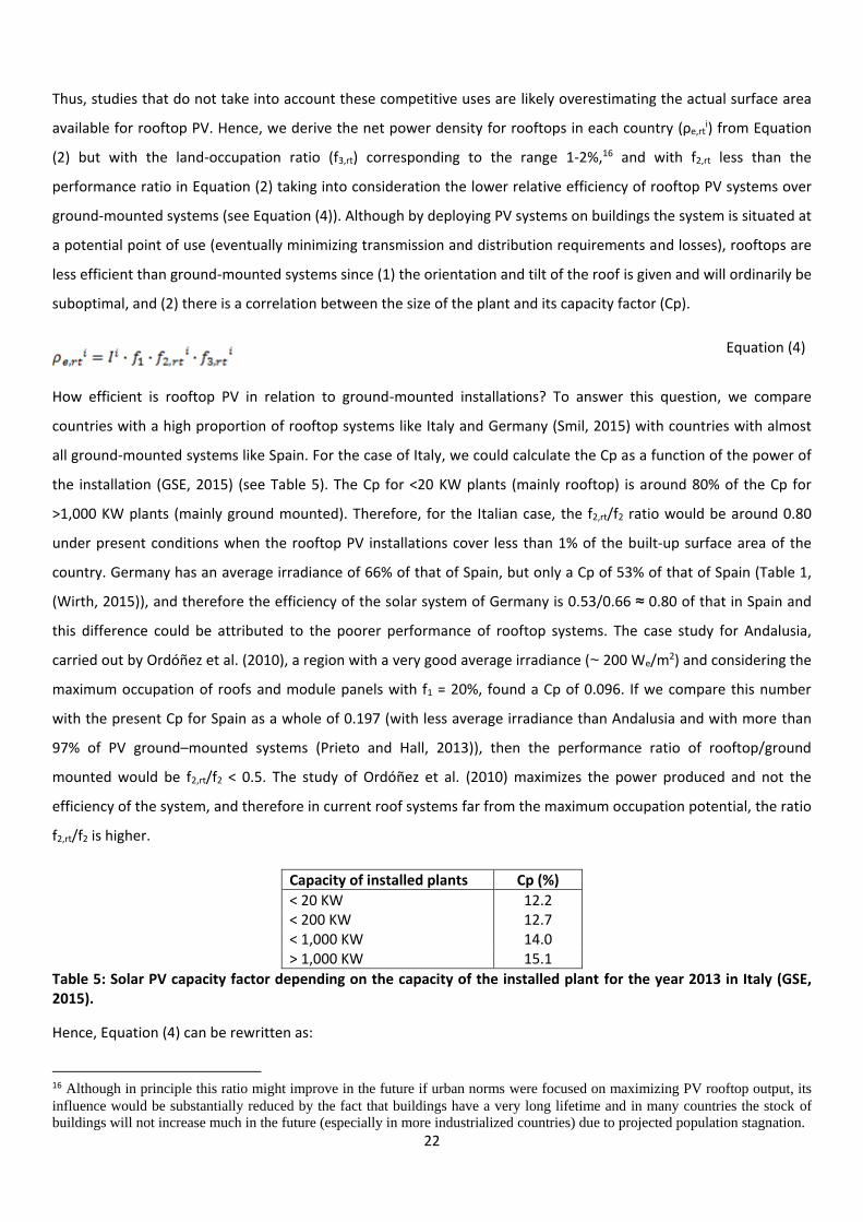
Thus, studies that do not take into account these competitive uses are likely overestimating the actual surface area
available for rooftop PV. Hence, we derive the net power density for rooftops in each country (ρe,rti) from Equation
(2) but with the land-occupation ratio (f3,rt) corresponding to the range 1-2%,16 and with f2,rt less than the
performance ratio in Equation (2) taking into consideration the lower relative efficiency of rooftop PV systems over
ground-mounted systems (see Equation (4)). Although by deploying PV systems on buildings the system is situated at
a potential point of use (eventually minimizing transmission and distribution requirements and losses), rooftops are
less efficient than ground-mounted systems since (1) the orientation and tilt of the roof is given and will ordinarily be
suboptimal, and (2) there is a correlation between the size of the plant and its capacity factor (Cp).
Equation (4)
How efficient is rooftop PV in relation to ground-mounted installations? To answer this question, we compare
countries with a high proportion of rooftop systems like Italy and Germany (Smil, 2015) with countries with almost
all ground-mounted systems like Spain. For the case of Italy, we could calculate the Cp as a function of the power of
the installation (GSE, 2015) (see Table 5). The Cp for <20 KW plants (mainly rooftop) is around 80% of the Cp for
>1,000 KW plants (mainly ground mounted). Therefore, for the Italian case, the f2,rt/f2 ratio would be around 0.80
under present conditions when the rooftop PV installations cover less than 1% of the built-up surface area of the
country. Germany has an average irradiance of 66% of that of Spain, but only a Cp of 53% of that of Spain (Table 1,
(Wirth, 2015)), and therefore the efficiency of the solar system of Germany is 0.53/0.66 ≈ 0.80 of that in Spain and
this difference could be attributed to the poorer performance of rooftop systems. The case study for Andalusia,
carried out by Ordóñez et al. (2010), a region with a very good average irradiance (~ 200 We/m2) and considering the
maximum occupation of roofs and module panels with f1 = 20%, found a Cp of 0.096. If we compare this number
with the present Cp for Spain as a whole of 0.197 (with less average irradiance than Andalusia and with more than
97% of PV ground–mounted systems (Prieto and Hall, 2013)), then the performance ratio of rooftop/ground
mounted would be f2,rt/f2 < 0.5. The study of Ordóñez et al. (2010) maximizes the power produced and not the
efficiency of the system, and therefore in current roof systems far from the maximum occupation potential, the ratio
f2,rt/f2 is higher.
Capacity of installed plants Cp (%)
< 20 KW 12.2 < 200 KW 12.7 < 1,000 KW 14.0 > 1,000 KW 15.1
Table 5: Solar PV capacity factor depending on the capacity of the installed plant for the year 2013 in Italy (GSE, 2015).
Hence, Equation (4) can be rewritten as:
16 Although in principle this ratio might improve in the future if urban norms were focused on maximizing PV rooftop output, its
influence would be substantially reduced by the fact that buildings have a very long lifetime and in many countries the stock of
buildings will not increase much in the future (especially in more industrialized countries) due to projected population stagnation.
23
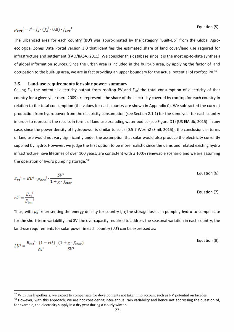
Equation (5)
The urbanized area for each country (BUi) was approximated by the category “Built-Up” from the Global Agro-
ecological Zones Data Portal version 3.0 that identifies the estimated share of land cover/land use required for
infrastructure and settlement (FAO/IIASA, 2011). We consider this database since it is the most up-to-date synthesis
of global information sources. Since the urban area is included in the built-up area, by applying the factor of land
occupation to the built-up area, we are in fact providing an upper boundary for the actual potential of rooftop PV.17
2.5. Land-use requirements for solar power: summary
Calling Erti the potential electricity output from rooftop PV and Etot
i the total consumption of electricity of that
country for a given year (here 2009), rti represents the share of the electricity covered by rooftop for each country in
relation to the total consumption (the values for each country are shown in Appendix C). We subtracted the current
production from hydropower from the electricity consumption (see Section 2.1.1) for the same year for each country
in order to represent the results in terms of land use excluding water bodies (see Figure D1) (US EIA db, 2015). In any
case, since the power density of hydropower is similar to solar (0.5-7 We/m2 (Smil, 2015)), the conclusions in terms
of land use would not vary significantly under the assumption that solar would also produce the electricity currently
supplied by hydro. However, we judge the first option to be more realistic since the dams and related existing hydro
infrastructure have lifetimes of over 100 years, are consistent with a 100% renewable scenario and we are assuming
the operation of hydro pumping storage.18
Equation (6)
Equation (7)
Thus, with representing the energy density for country i, χ the storage losses in pumping hydro to compensate
for the short-term variability and SVi the overcapacity required to address the seasonal variation in each country, the
land-use requirements for solar power in each country (LUi) can be expressed as:
Equation (8)
17 With this hypothesis, we expect to compensate for developments not taken into account such as PV potential on facades. 18 However, with this approach, we are not considering inter-annual rain variability and hence not addressing the question of, for example, the electricity supply in a dry year during a cloudy winter.
24
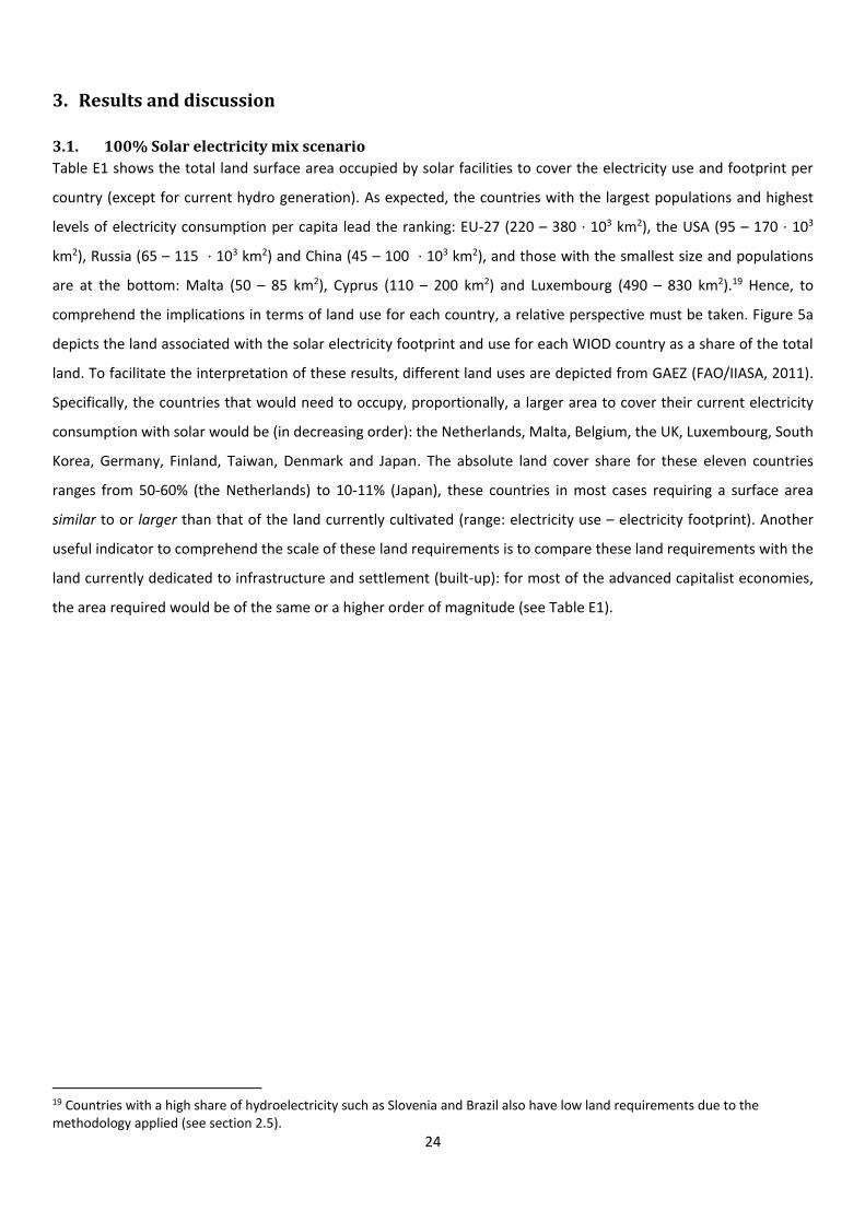
3. Results and discussion
3.1. 100% Solar electricity mix scenario
Table E1 shows the total land surface area occupied by solar facilities to cover the electricity use and footprint per
country (except for current hydro generation). As expected, the countries with the largest populations and highest
levels of electricity consumption per capita lead the ranking: EU-27 (220 – 380 · 103 km2), the USA (95 – 170 · 103
km2), Russia (65 – 115 · 103 km2) and China (45 – 100 · 103 km2), and those with the smallest size and populations
are at the bottom: Malta (50 – 85 km2), Cyprus (110 – 200 km2) and Luxembourg (490 – 830 km2).19 Hence, to
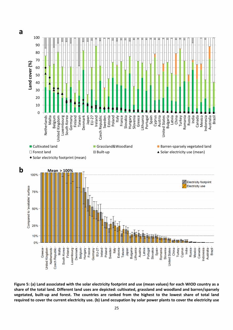
comprehend the implications in terms of land use for each country, a relative perspective must be taken. Figure 5a
depicts the land associated with the solar electricity footprint and use for each WIOD country as a share of the total
land. To facilitate the interpretation of these results, different land uses are depicted from GAEZ (FAO/IIASA, 2011).
Specifically, the countries that would need to occupy, proportionally, a larger area to cover their current electricity
consumption with solar would be (in decreasing order): the Netherlands, Malta, Belgium, the UK, Luxembourg, South
Korea, Germany, Finland, Taiwan, Denmark and Japan. The absolute land cover share for these eleven countries
ranges from 50-60% (the Netherlands) to 10-11% (Japan), these countries in most cases requiring a surface area
similar to or larger than that of the land currently cultivated (range: electricity use – electricity footprint). Another
useful indicator to comprehend the scale of these land requirements is to compare these land requirements with the
land currently dedicated to infrastructure and settlement (built-up): for most of the advanced capitalist economies,
the area required would be of the same or a higher order of magnitude (see Table E1).
19 Countries with a high share of hydroelectricity such as Slovenia and Brazil also have low land requirements due to the methodology applied (see section 2.5).
25
a
b Mean > 100%
0
10
20
30
40
50
60
70
80
90
100
Ne
the
rlan
ds
Mal
taB
elgi
um
Un
ite
d K
ingd
om
Luxe
mb
ou
rgSo
uth
Ko
rea
Ger
man
yFi
nla
nd
Taiw
anD
en
mar
kJa
pan
EU-2
7Ir
elan
dC
zech
Rep
ub
licSw
ed
enEs
ton
iaP
ola
nd
Ital
yFr
ance
Slo
vaki
aH
un
gary
Slo
ven
iaG
reec
eLi
thu
ania
Po
rtu
gal
Spai
nC
ypru
sA
ust
ria
Un
ite
d S
tate
sB
ulg
aria
Latv
iaC
hin
aTu
rke
yR
om
ania
Ru
ssia
Ind
iaC
anad
aM
exi
coIn
do
nes
iaA
ust
ralia
Bra
zil
Lan
d c
ove
r (%
)
Cultivated land Grassland&Woodland Barren-sparsely vegetated land
Forest land Built-up Solar electricity use (mean)
Solar electricity footprint (mean)
Figure 5: (a) Land associated with the solar electricity footprint and use (mean values) for each WIOD country as a share of the total land. Different land uses are depicted: cultivated, grassland and woodland and barren/sparsely vegetated, built-up and forest. The countries are ranked from the highest to the lowest share of total land required to cover the current electricity use. (b) Land occupation by solar power plants to cover the electricity use
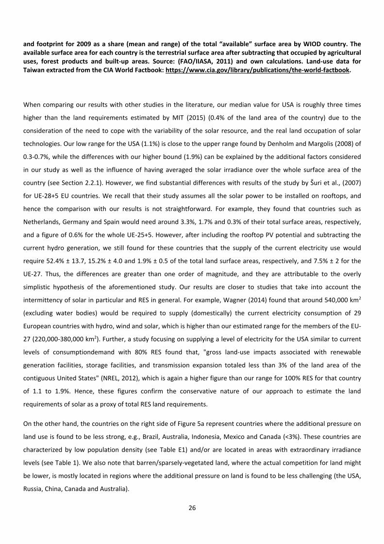
26
and footprint for 2009 as a share (mean and range) of the total “available” surface area by WIOD country. The available surface area for each country is the terrestrial surface area after subtracting that occupied by agricultural uses, forest products and built-up areas. Source: (FAO/IIASA, 2011) and own calculations. Land-use data for Taiwan extracted from the CIA World Factbook: https://www.cia.gov/library/publications/the-world-factbook.
When comparing our results with other studies in the literature, our median value for USA is roughly three times
higher than the land requirements estimated by MIT (2015) (0.4% of the land area of the country) due to the
consideration of the need to cope with the variability of the solar resource, and the real land occupation of solar
technologies. Our low range for the USA (1.1%) is close to the upper range found by Denholm and Margolis (2008) of
0.3-0.7%, while the differences with our higher bound (1.9%) can be explained by the additional factors considered
in our study as well as the influence of having averaged the solar irradiance over the whole surface area of the
country (see Section 2.2.1). However, we find substantial differences with results of the study by Šuri et al., (2007)
for UE-28+5 EU countries. We recall that their study assumes all the solar power to be installed on rooftops, and
hence the comparison with our results is not straightforward. For example, they found that countries such as
Netherlands, Germany and Spain would need around 3.3%, 1.7% and 0.3% of their total surface areas, respectively,
and a figure of 0.6% for the whole UE-25+5. However, after including the rooftop PV potential and subtracting the
current hydro generation, we still found for these countries that the supply of the current electricity use would
require 52.4% ± 13.7, 15.2% ± 4.0 and 1.9% ± 0.5 of the total land surface areas, respectively, and 7.5% ± 2 for the
UE-27. Thus, the differences are greater than one order of magnitude, and they are attributable to the overly
simplistic hypothesis of the aforementioned study. Our results are closer to studies that take into account the
intermittency of solar in particular and RES in general. For example, Wagner (2014) found that around 540,000 km2
(excluding water bodies) would be required to supply (domestically) the current electricity consumption of 29
European countries with hydro, wind and solar, which is higher than our estimated range for the members of the EU-
27 (220,000-380,000 km2). Further, a study focusing on supplying a level of electricity for the USA similar to current
levels of consumptiondemand with 80% RES found that, "gross land-use impacts associated with renewable
generation facilities, storage facilities, and transmission expansion totaled less than 3% of the land area of the
contiguous United States" (NREL, 2012), which is again a higher figure than our range for 100% RES for that country
of 1.1 to 1.9%. Hence, these figures confirm the conservative nature of our approach to estimate the land
requirements of solar as a proxy of total RES land requirements.
On the other hand, the countries on the right side of Figure 5a represent countries where the additional pressure on
land use is found to be less strong, e.g., Brazil, Australia, Indonesia, Mexico and Canada (<3%). These countries are
characterized by low population density (see Table E1) and/or are located in areas with extraordinary irradiance
levels (see Table 1). We also note that barren/sparsely-vegetated land, where the actual competition for land might
be lower, is mostly located in regions where the additional pressure on land is found to be less challenging (the USA,
Russia, China, Canada and Australia).
27
However, these results must also be put in context: the degree of land competition will critically depend on the use
of land at the country level. Given this, we define for each country its “land availability”, consisting of the terrestrial
land that is currently neither being used by the primary sector (arable land, permanent crops, permanent meadows
and pastures and productive forest area (FAOSTAT, 2015)) nor built-up (FAO/IIASA, 2011). Furthermore, we consider
an additional land use for a biodiversity buffer to safeguard the resilience and stability generated by biodiversity. We
apply here the value of 12% of the territory as considered in the Brundtland Report and for the calculation of the
standard ecological footprint (Wackernagel et al., 2002; WCED, 1987). This value is a conservative lower bound,
which has been strongly criticized as being unable to a ensure an effective protection of biodiversity (Vačkář, 2012).
For example, the UNEP and IUCN give 17% as a reference value (Juffe-Bignoli et al., 2014), while Soulé and Sanjayan
(1998) argued for a minimum share of 25-50%.
This definition of land availability must be taken as a first conservative approximation, since its availability would in
fact be reduced by many other factors including orography (e.g., mountains), protected areas (e.g., in the EU-27, an
average of around 27% of the land is protected, which is more than twice our 12% assumption), and locations with
suboptimal resources, that would more than offset other positive factors such as eventual productivity gains in the
agriculture sector (see Deng et al., (2015) and Farthing et al., (2016)). The estimated land availability per country is
depicted in Figure F1.
Taking into account this definition of land availability, the pressure on land would be very high in many countries,
with some of them even requiring more surface than the estimated available land (see Figure 5b). The latter would
be the case (in mean electricity use values) for: Greece (not even having enough available land for the assumed
biodiversity buffer), the UK (almost 7x), the Netherlands (over 3x), and Czech Republic (over 2x), as well as Malta,
South Korea, Finland, Luxembourg, Denmark and Belgium (between all and 2x their available surface). The EU-27 as
a whole would require around 50% of its available land. In fact, few advanced capitalist economies would require
less than a 10%20 of the available surface such as Portugal, Slovakia, Spain and the USA (below 5 and 10%), as well as
Cyprus, Canada and Australia (below 5%). For Austria, Latvia, Romania and Slovenia, the land requirements in this
scenario are also below 10%: however, for these countries, hydroelectricity contributed over 35% of the electricity
consumption in 2009 (see Figure D1). Our results help to explain why, when solar is scaled up, parks are often being
located in agricultural areas and biodiversity hotspots (e.g., (Bocca et al., 2015; Hernandez et al., 2015; Squatrito et
al., 2014)).
In relation to the differences in land-use requirements when accounting for the electricity demanded from the
territorial and the consumption perspective, the estimation of the electricity footprint worsens the situation for
countries with a higher electricity footprint than use (see Section 2.1). For example, in median values, the
20 This 10% “threshold” has been chosen arbitrarily, and it is far beyond the scope of this paper to state which levels of solar occupation would be excessive or unfeasible in practice. That would require analysis of the extent to which additional pressure on current land uses would affect agricultural production (i.e., crop prices) and eventually be an additional driver for deforestation, among other negative effects.

28
Netherlands would require almost an additional 8% of total land (from 52 to 60%), UK an additional 6% (from 26 to
32%) and Denmark an additional 4.5% (from 12.5 to 17%). For other countries like Spain, characterized by an
electricity footprint notably higher than the electricity use, higher irradiance levels mitigate this difference, Spain
requiring only an additional 0.3% (from 1.9% to 2.2%) in terms of total land and 1.2% (from 8.6 to 9.8%) in terms of
available land. At the EU-27 aggregate level, the additional land-use requirements when computing the electricity
footprint would be 0.6% for total land and almost 4% for available land. At the other extreme, we find countries
whose land requirements are substantially reduced when taking into account the net embedded electricity footprint
in trade. These include exporting countries such as Taiwan (from 13.6 to 9.1% in terms of electricity consumption).
3.2. 100% Solar final energy mix scenario
We replicate the analysis, this time computing the land requirements to cover the final energy use of each country.
In terms of total land-use (Figure 6a), the first notable finding is that for six countries the supply of final energy use
from solely solar energy would be physically unfeasible: the Netherlands, Luxembourg, Malta, Belgium, the UK and
Denmark. Other countries would require vast amounts of land that would likely also make this scenario unfeasible in
practice: most notably Germany, South Korea, Taiwan and Finland (over 50% of the total country land); but also
Japan, Ireland, Czech Republic, Sweden, Poland, Estonia and Italy (over 30%). For the whole EU-27, we find that land
requirements would reach 45.5% ± 11.5 of the total land. In this sense, MacKay’s (2013) results are confirmed. The
list of countries requiring a less than 10% share of total land is: Spain, the USA, Romania, China, and Turkey (above
5%); as well as Bulgaria, Russia, India, Canada, Indonesia, Mexico, Brazil and Australia (below 5%). Table E2 shows
the total land surface area (km2) occupied by solar facilities per country and the associated land per capita
(m2/person) in terms of final energy use and footprint.
Analyzing the results in terms of “available” land, over 20 WIOD countries would require more than the estimated
available surface. These countries are most of the EU-27 member states (all except for Lithuania, Slovakia, Romania,
Portugal, Spain, Bulgaria, Slovenia and Cyprus) and South Korea. Seven of them would require a surface area at least
an order of magnitude higher than the current estimated available land (Greece, the UK, Netherlands, Luxembourg,
Czech Republic, Malta and Denmark). The EU-27 would require more than twice its estimated available surface area.
Japan would require around 80%. On the other hand, the only countries with requirements 10% of the available land
would be Russia, Indonesia, Mexico, Canada, Brazil and Australia. The USA, Cyprus, Canada and Australia would be
the only advanced capitalist countries requiring less than 25% of the available land.
In terms of final energy footprint (Figure 6b), we observe similar trends to those found for electricity footprint:
advanced capitalist economies (e.g., Slovenia, Spain, Japan, Spain and Portugal) would require a larger area to cover
their energy footprint than to cover their energy use (+11.2%, +9.5%, +9% and +6%, respectively), while exporting
countries such as Taiwan (-37%), and BRIC countries such as China and Russia would reduce their land needs (-4%
and -2%, in terms of available land).

29
a
b Mean > 100%
Mean > 100%
0
10
20
30
40
50
60
70
80
90
100N
eth
erl
and
sLu
xem
bo
urg
Mal
taB
elgi
um
Un
ite
d K
ingd
om
De
nm
ark
Ger
man
ySo
uth
Ko
rea
Taiw
anFi
nla
nd
Jap
anIr
elan
dEU
-27
Cze
ch R
epu
blic
Swe
den
Po
lan
dEs
ton
iaIt
aly
Au
stri
aSl
ova
kia
Fran
ceH
un
gary
Slo
ven
iaLa
tvia
Lith
uan
iaG
reec
eP
ort
uga
lC
ypru
sSp
ain
Un
ite
d S
tate
sR
om
ania
Ch
ina
Turk
ey
Bu
lgar
iaR
uss
iaIn
dia
Can
ada
Ind
on
esia
Me
xico
Bra
zil
Au
stra
lia
Lan
d c
ove
r (%
)
Cultivated land Grassland&Woodland Barren-sparsely vegetated land
Forest land Built-up Solar electricity use (mean)
Solar electricity footprint (mean)
Figure 6: (a) Land associated with the solar final energy footprint and use (mean values) for each WIOD country as a share of the total land. Different land uses are depicted: cultivated, grassland and woodland and barren/sparsely vegetated, built-up and forest. The countries are ranked from the highest to the lowest share of
30
total land required to cover the current electricity use. (b) Land occupation by solar power plants to cover the electricity use and footprint for 2009 as a share (mean and range) of the total “available” surface area by WIOD country. The available surface area for each country is the terrestrial surface area after subtracting the areas for agricultural uses, forest products and built-up areas. Source: (FAO/IIASA, 2011) and own calculations. Land-use data for Taiwan extracted from the CIA World Factbook: https://www.cia.gov/library/publications/the-world-factbook.
Studies proposing a 100% total energy mix supplied by RES for individual countries are less common than those
focusing on the transition solely in the electricity sector. This might be due to the great complexity of designing
models that encompass all the final energy types in an economy, as well as the fact that the electricity sector is
usually seen as the easiest sector to decarbonize (e.g. (IPCC, 2014)). Among the exceptions are several studies
applying the EnergyPLAN model. However, comparisons are not straightforward, since this model does not include a
land-use module. For example, Lund and Mathiesen (2009) find for Denmark that a 100% RES system would require
a flow of biomass that would be twice the domestic potential of the estimated residual biomass resources including
waste, acknowledging that this scenario would require a deep reorganization of land use at the country level (or rely
on imports). A similar analysis for Ireland lead to analogous conclusions (Connolly et al., 2011). These findings are in
accordance with our results, namely, that the land requirements for a 100% total energy mix supplied by RES would
require around 30-50% and 30-110% of the total surface of the country, in the cases of Ireland and Denmark
respectively, and over 100% for the available land for both countries. In fact, the land footprint in 2008 is estimated
to be of the same order of magnitude as and twice the territorial area of Ireland and Denmark respectively (Arto et
al., 2012). These figures indicate that even in the event of internal reorganization of land use, in the future, it would
not be possible to cover both energy and food needs domestically in these countries in a 100% total energy mix
scenario at current consumption levels. A study for UK analyzing the implications of meeting just 15% of final energy
demand with RES by 2020 concluded that a large part of the RES needs should be covered by imports (Ward and
Inderwildi, 2012). Hence, these analyses are consistent with the results we obtained indicating that, in the future,
there might be a trade-off between land for food, land for energy and land for biodiversity conservation in certain
countries, implying also trade-offs between food and energy security. Of course, these trade-offs will impact other
regions of the globe through indirect land use changes, as it has already happened with the promotion of biofuels in
the EU (Laborde, 2011; Valin et al., 2015). Nonetheless, quantitative analysis of these dynamics is not described in
the literature, most energy models not including a comprehensive representation of the land-use system (Otto et al.,
2015).
The literature focusing on the transition to a 100% RES system at a globally aggregated level usually finds that land
requirements will not pose significant constraints on this transition (García-Olivares, 2016; Greenpeace et al., 2015;
Jacobson and Delucchi, 2011; WWF, 2011). For example, Jacobson and Delucchi (2011) find that just an additional
0.41% of the global land area (1% including spacing area) would be required for a global 100% RES system. García-
Olivares (2016) finds a similar footprint of ~1% of global continental surface area for PV and CSP plants in his global

31
100% RES mix proposal. Our results cannot be directly compared with these globally aggregated analyses, which
assume that large quantities of electricity/energy could be technically transported at a continental scale between
areas with high levels of renewable resources (e.g., solar from deserts and wind from marine platforms) to the
regions of consumption, which are often distant. Nevertheless, we judge that geopolitical and economic barriers, as
well as concerns over energy and food security, will effectively pose significant constraints on the setting up of such
large-scale intercontinental infrastructure (see section 4.1 for a discussion of this assumption in comparison with the
“country’s self-sufficiency” approach followed in this study).
4. Assessment of assumptions and uncertainties in estimating the land-use
requirements of the transition to RES
In this section, five central assumptions of the analysis are assessed: the countries’ self-sufficiency in electricity/final
energy consumption and 100% solar share (section 4.1), the combination of static and dynamic approaches (section
4.2), the estimation of solar power density at country level (section 4.3), the implications of not accounting for the
energy return on energy inverted (EROI) (section 4.4) and the estimation of PV potential in buildings (section 4.5).
4.1. Country’s self-sufficiency in electricity/final energy and 100% solar share
Most countries in the world are connected to the grid of neighboring countries, thereby allowing for some degree of
electricity trade. While some countries are an “energetic island” (e.g., Australia, Japan, China, and Turkey), others
export (e.g., Bulgaria, Canada, and France) or import (e.g., Italy, Hungary, and Portugal) considerable amounts of
electricity. The external dependence of total energy is usually high for advanced capitalist economies due to the
dependence on fossil fuel imports (UN Comtrade, 2015). However, improving energy security is a key policy
objective for most governments, and self-sufficiency through the increase in RES production is one of the commonly
cited instruments (Johansson, 2013; US ACT, 2007). The EU members are not an exception, although representing a
special case due to the planned progressive integration of each members’ systems into a pan-European scheme (the
“Energy Union”) (European Commission, 2014)), eventually allowing for greater electricity trade. For this reason, the
results are reported here also at the EU-27 level. In any case, the process is slow: a minimum interconnection target
(which should be achieved by 2030) has been set at 15% of installed electricity production capacity of the member
states, well below the required levels of interconnection to balance supply and demand at the European level
(Wagner, 2014).
There is another potential scale of integration discussed theoretically in the literature that goes beyond the regional
scale: the intercontinental scale. Many studies focusing on the technical feasibility of a global 100% renewable mix
propose these interconnections (in combination with other strategies such as smart grids, storage or demand
management) as a solution to renewable intermittence and fluctuation, as well as to the unequal distribution of the
resource (e.g., high solar irradiance near the tropics and wind at northern latitudes and on sea platforms). In this
way, the increase in transportation losses would be largely offset by the use of locations where the available
resource is more abundant (Armaroli and Balzani, 2011; García-Olivares et al., 2012; Jacobson and Delucchi, 2011;

32
Trainer, 2013a). Although several projects have been proposed, none is currently under way (Breyer et al., 2015;
DESERTEC, 2003; Gulagi et al., 2017). For example, the DESERTEC project aiming to harness solar energy from
deserts, producing large amounts of electric power by CSP plants based in Northern Africa and the Arabian
Peninsula, and transmit it through high-voltage direct current (HVDC) transmission lines to Europe (DESERTEC, 2003).
Its connection with the electricity generated by PV, wind, hydro, geothermal and biomass in European countries
would lead to an integrated regional framework (Armaroli and Balzani, 2011). However, these kinds of projects are
very sensitive to geopolitical circumstances and depend on gigantic investments. In fact, the DESERTEC consortium
dissolved some years ago and there are no imminent prospects for its reactivation (Smil, 2015). On the other hand,
although significant new construction of HVDC lines is currently under way (particularly in China and Brazil), very
little of the new capacity actually crosses country borders except in the EU. The feasibility of large intercontinental
grids operating within the next few decades critically depends on future global societal pathway uncertainty. Under
pathways characterized by an intensification of globalization and market integration processes (including
international trade growth), these forecasts may prove valid. However, under scenarios dominated by fragmentation
and regionalization of the relationships between countries, the functioning of these systems would be unrealistic
(MEA, 2005; Raskin et al., 2002). In fact, these regional and intercontinental interconnection processes require that
the participants collaborate to share and commonly manage their resources. Alternatively, this could also be
achieved through force, with the strongest countries seizing locations with abundant renewable resources from
countries not willing to collaborate. On the other hand, large intercontinental grids of thousands of kilometers and
large areas dedicated to RES generation systems in foreign territories might also be an “easy” target to paralyze the
economic activity of the importing regions. Moreover, given the lower power densities of RES in relation to fossil
fuels, the surface required for RES generation systems is much higher, and hence, the geographical area to be
secured by importing regions substantially increases, thereby substantially increasing their vulnerability (Lilliestam
and Ellenbeck, 2011)
A renewable mix portfolio would mitigate the variability of the solar resource, eventually reducing the need for
storage and overcapacity considered in this analysis. For example, in Europe, the annual cycles of wind and PV are
partially complementary since the lower solar irradiance in winter is generally balanced by increased wind (and vice
versa in the summer). There is also generally a trade-off between the installation of additional generation capacities
and storage capacities to balance the intermittence of resources that is not captured by our approach (Armaroli and
Balzani, 2011; François et al., 2016; Wagner, 2014; Weitemeyer et al., 2015). However, this complementarity is far
from perfect. In any region there is a (low) probability of extreme combinations in the availability of natural
resources, such as no wind over large parts of Europe during the winter. Moreover, there can be extreme annual
variations in the availability of natural resources; for instance, the output of wind turbines in any given area can vary
by up to 30% from one year to the next (Brower et al., 2013; Li et al., 2010). With hydroelectricity covering currently
a mere 15% of the current global electricity consumption and already being close to its technical potential in many
33
countries (IPCC, 2011), only wind could cover a substantial share of the remainder in a sustainable way. Moreover,
wind generation could moderate the impact in terms of land use since, despite its lower power density, both
offshore deployment and double land use are possible. On the other hand, technical (Lenzen, 2010) and biophysical
limitations (de Castro et al., 2011; Miller et al., 2011) hinder large-scale deployment of wind energy. We have chosen
to give priority to overcapacity (following a conservative approach, see Section 2.3) rather than storage, since
economic options for large-scale and seasonal storage are currently neither technically available nor foreseen at the
required scale. Moreover, storage losses would be higher than considered here, as hydro pumping cannot be
generalized (MacKay, 2013; Trainer, 2012). Other sources of variability such as low rain years have not been
considered; and, by taking the monthly irradiance average, we are not accounting for short-term solar variability
(i.e., over hours, days, weeks). Finally, we have not allowed for the fact that demand peaks at certain times of day at
levels much higher than the average (Trainer, 2013a), conservative estimates of these peaks being +30%, while other
studies have yielded estimates several times higher. Coping with these factors would require greater levels of
storage and/or overcapacity (higher SV). Moreover, the system should be designed for the minimum of all the
energies in the mix, that might well be close to the minimum in a full 100% solar system (Trainer, 2012).
4.2. Static vs. dynamic projections
The proposed analysis follows a hybrid approach by combining static data (i.e., electricity consumption values for
2009) with dynamic factors (e.g., the uncertainty range for the future evolution of cell efficiency). The objective of
this approach is double: on the one hand, to replicate the methodology followed in previous studies to allow
comparability (Denholm and Margolis, 2008; Šúri et al., 2007), and on the other, to perform a vulnerability study in
order to identify countries for which the objective of high solar power deployment might be unfeasible due to land
constraints. This approach does not fully correspond with an “extreme scenario” when considering the expected
increases in electricity and energy production globally for the coming decades (Armaroli and Balzani, 2011; WEO,
2014). In particular, emerging economies are expected to substantially increase their income and population levels in
the coming decades. Let us take the case of India. Our estimated land requirements in terms of total land use seem
relatively low for both covering electricity (0.4% ± 0.2) and final energy (3.8% ± 1.1) consumption. However, its
population density is very high (over 400 people per km2 of terrestrial land), a large share of their land being
required to produce feedstock (almost 60%, see Figure 5a) or built up (~7%). Hence, in terms of land availability the
situation worsens substantially, especially in terms of final energy (26.1% ± 7.5). Population growth (projected to be
+30% to 2050 (UN, 2015)) combined with the expected increase in energy consumption (currently around a third of
the global average, see Figure 1) are likely to drive land requirements to unfeasible levels. Similar reasoning could be
applied to other emerging countries such as China and Nigeria (Deng et al., 2015).
In relation to the estimated “land availability”, it could be argued that improvements in agricultural yield might to
some extent compensate for increases in food demand due to population growth and diet shift in the future.

34
However, after decades of improvement due to agricultural intensification (based on inputs such as fertilizers,
energy, water and capital equipment), yields might be approaching biophysical limits in some developed countries,
and could stagnate for socio-economic reasons in developing countries (Alston et al., 2009; Grassini et al., 2013;
Sands et al., 2014).
4.3. Estimation of solar power density at the country level
Various factors affect the estimation of the solar density for each country (see Section 2.2.1). The consideration of
country average irradiance levels might be seen as a conservative assumption since areas with more irradiance are
likely to be occupied more intensively. On the other hand, there are other important variables that influence the
location of new power plants such as proximity to the consumer demand and existing electricity transport
infrastructure. This is the case of, for example, Australia and Germany, where the locations used are mainly sub-
optimal in terms of irradiance. However, we tried to compensate for this effect by selecting favorable parameters for
the overcapacity factors (e.g., SV, CRC, etc.). In some cases, these parameters are even unrealistic since they
correspond to locations of high mountains (i.e., less cloud cover, e.g., China CRC) or protected areas.
As stated above, large solar parks usually have higher power density levels than smaller ones. Hence, factors such as
existing promotion policies and development frameworks will determine the number of each to be installed (i.e.,
planned economy, investment of large companies or small cooperatives or producers, self-production, etc.).
Moreover, if land competition is to play a relevant role in future solar deployment, the factor f3 might even decrease
due to the need to adapt to the accessible fields.
4.4. Not accounting for EROI
The EROI is defined as the ratio of the amount of usable energy acquired from a particular energy resource (Eout) to
the amount of energy spent obtaining that energy resource (Ein). Thus, accounting for the EROI of the solar PV
systems would increase the required installed capacity to deliver the same output of net energy to the society.
Defining r as the relative losses (Ein/Eout, see eq. 10), the total capacity to install in order to compensate for the
energy invested would be given by the series 1+r2+r3+…, which is the Taylor series of 1/(1-r) (see eq. 11).
Equation (9)
Equation (10)
Equation (101)

35
An examination of the EROI literature on solar PV energy generation shows differences in the assumptions,
parameters and methodologies employed (Hall et al., 2014). Assuming a conventional value of 10:1 and applying the
Eq. 10, an overcapacity of 10/(10-1)-1≈11% would be then required in an hypothetical 100% solar energy system.
The extended EROI (EROIext) broadens the conventional analysis by considering all the energy used to create and run
a PV facility, including the fabrication of the PV modules (more than 95% of the power used for the manufacture of
solar PV cells being electricity (Briner, 2009)), but also for the energy required for transportation, installation,
maintenance, and all the other required energy inputs. The estimation of the EROIext of PV systems range 2 to 3:1
(Hall et al., 2014), which would translate into overcapacities of 50% to 100%. Hence, accounting for the EROI factor
would substantially increase the land requirements obtained in this analysis.
4.5. PV potential in buildings
As pointed out in Section 2.4, there is substantial heterogeneity in the literature in relation to the methods applied
(achieving a different geographical coverage and levels of spatial resolution) and the results obtained. Our study
incorporates assumptions about storage, seasonal variability and competing uses that are rarely taken into account
in research in this field. It is therefore challenging to compare our results (see Appendix C) with those of other
studies. The estimated PV rooftop potential seems to be in accordance with the GIS-based studies considered (e.g.,
for Spain, Izquierdo et al. (2011) having found that rooftop PV could cover around 4% of the total electricity demand,
which is within our range, 2.2-7.4%, including hydro), while our figures are substantially lower than those obtained
by constant-value methods (e.g., Defaix et al. (2012) and Paidipati et al. (2008) having reported potential shares of
over 20% of the annual electricity demand for the EU-27 and USA). Further research is required to characterize the
variability in these methods to reduce the uncertainties in current estimates, as has already been done, for example,
for PV and CSP technologies (Horner and Clark, 2013). Further, the method applied does not escape the fact that
there is a large uncertainty in the estimation of urban/built-up areas, with differences of an order of magnitude
(Schneider et al., 2009). In relation to this, the GAEZ database (FAO/IIASA, 2011) used is the most recent attempt to
provide a consistent estimate across different countries, and the global built-up area is in the upper range of the
literature (around 1.5 million km2) (Schneider et al., 2009).
5. Conclusions In this work, we have analyzed the biophysical feasibility and potential vulnerabilities in the transition to renewable
energies focusing on the land requirements for 100% solar energy scenarios for 40 countries considering two issues
that are not usually considered in the literature: (1) the need to cope with the variability of the solar resource, and
(2) the real land occupation of solar technologies. The exercise performed shows that, for many advanced capitalist
economies, the land requirements over the total terrestrial surface area to supply current electricity consumption
would be substantial, the situation being especially challenging for those located in northern latitudes with high
population densities and high electricity consumption per capita such as the Netherlands, Belgium, the UK,
Luxembourg, South Korea, Germany, Finland, Taiwan, Denmark and Japan (10-50%). Moreover, accounting for the

36
electricity footprint, i.e., for the net energy embodied in international trade, tends to worsen the situation of these
countries, increasing the land requirements to 11-60%. To assess the implications in terms of land competition, we
have defined a land availability factor based on current land use and including a biodiversity buffer. With this
indicator, the list of vulnerable countries enlarges substantially (e.g., the EU-27 would require around 50% of their
available land), while few advanced capitalist economies would require low shares of the estimated available land
(e.g., Canada and Australia, < 1%).
Specifically, the consideration of circumstances not usually taken into account in the literature such as the need for
redundant capacity to ensure sufficient winter supply and the real land-occupation factor of solar power plants
produces results more challenging in terms of land requirements than previously found (Denholm and Margolis,
2008; Jacobson and Delucchi, 2011; Šúri et al., 2007). In particular, assertions about the practical unlimited nature of
the solar potential should be reconsidered (e.g., (IPCC, 2011; Rogner et al., 2012)). In fact, our results help to explain
why, when solar is scaled up, parks are often being located in agricultural areas and biodiversity hotspots, namely,
that this is a palpable example of the finiteness of the biosphere, i.e., of the “full world” to use the popular
expression coined by Daly (2005).
The explorative exercise to examine the implications of a 100% solar energy mix for the same set of countries reveals
the marked implications of the transition from concentrated fossil energies (i.e., “mines”) to distributed (over the
Earth’s surface) RES. The results, that must be interpreted as order of magnitude estimates, due to the limitations
and uncertainties of the analysis, indicate that the transition to domestically produced RES maintaining the current
levels of energy consumption could be physically unfeasible for many countries: in particular, the Netherlands,
Luxembourg, Belgium, the UK, Denmark, Germany, South Korea, Taiwan, Finland, Japan, Ireland, Czech Republic,
Sweden, Poland, Estonia and Italy would require over 30% of their total land area (over 50% for the whole EU-27).
Due to the biophysical restrictions on solar, these countries will have to rely on other domestic renewable sources
(mainly wind and eventually biomass) or imports in their path to a 100% RES system. Although concerns over the
potential land scarcity provoked by a full transition to RES have been already pointed out from a theoretical point of
view (Johansson, 2013; Rao and Sastri, 1987; Scheidel and Sorman, 2012), currently available energy models are
unable to properly capture the trade-offs between energy and food security, as well as biodiversity conservation, in
the context of 100% RES scenarios. We attempt to contribute to the discussion by a rough quantification of potential
implications. Specifically, by providing a ranking, we identify countries with particularly high vulnerabilities.
In this context, emerging countries might seem less vulnerable. However, if the projections of electricity and energy
consumption growth, on the one hand, and the population increase, on the other, prove to be correct, such
countries may suffer similar land pressures in the future to those currently on the advanced capitalist economies.
Indeed, the pressures might be even greater, if the current structure of international trade, where they export
substantial amounts of embodied energy, is not modified.

37
Thus, the transition to RES maintaining the current levels of energy consumption might create new vulnerabilities
and/or reinforce existing ones in terms of biodiversity conservation, energy (and food) security and sovereignty, with
the potential to intensify imperialist geopolitics to grab land and seize resources from other countries. It seems likely
that, without profound changes in the level and management of energy demand (adaptation to the natural
fluctuations in the availability of renewables, consumption reduction and equity at the global level) and the socio-
economic system (i.e., the growth paradigm), the transition to renewables will substantially increase the competition
for land globally.
Finally, we recall that the analysis performed must be understood as a vulnerability study of the unavoidable path to
a 100% RES system for all countries. Future work could be focused on (1) dynamic developments, (2) expanding the
potential constraints that may further reduce PV feasibility (e.g., material availability (García-Olivares et al., 2012; Lo
Piano and Mayumi, 2016)), (3) analyzing the feasibility and land requirements of different 100% RES mixes, which
has to be approached at a country level and with a different methodology,21 and (4) improving the methods to
represent the land availability and competition between different uses in existing energy models. In particular, GIS-
based methods or integrated assessment models that include the interaction between the energy system and land-
use changes could substantially contribute to advance in these directions.
Acknowledgements The authors gratefully acknowledge Ignacio Cazcarro for performing the calculations with GIS. This work has been
partially developed under the MEDEAS project, funded by the European Union’s Horizon 2020 research and
innovation programme under grant agreement No 691287. This work was partially developed within the ESPON
Study on “Possible European Territorial Futures” (Contract No EE/SO1/007/2016).
Appendix A: Electricity and final energy consumption by country for 2009
Electricity use Electricity footprint Final energy use Final electricity footprint
MWh/year/person MWh/year/person MWh/year/person MWh/year/person
Australia 11.9 12.5 51.0 59.1
Austria 7.6 9.0 41.3 50.7
Belgium 8.2 8.9 52.0 48.7
Brazil 2.6 2.6 13.5 13.6
Bulgaria 4.9 4.3 15.1 15.2
Canada 16.9 16.3 79.2 75.6
China 2.8 2.2 14.6 12.5
Cyprus 6.6 9.1 32.7 42.9
Czech Republic 6.5 6.1 31.8 30.0
Denmark 6.2 8.4 53.7 47.8
21 The methodology applied here cannot straightforwardly be extended for wind since bottom-up analyses violate the Principle of Conservation of Energy (de Castro et al., 2011; Miller et al., 2011).

38
Estonia 6.6 6.0 28.8 29.0
Finland 15.8 14.2 62.4 59.9
France 7.9 9.1 31.0 40.2
Germany 7.0 7.7 37.6 44.0
Greece 5.8 7.9 28.9 35.1
Hungary 4.1 4.5 22.4 24.2
India 0.8 0.8 4.6 4.8
Indonesia 0.7 0.8 7.6 7.7
Ireland 6.4 8.3 36.4 46.3
Italy 5.6 6.6 27.3 35.0
Japan 8.2 8.9 35.0 38.8
South Korea 9.4 7.9 43.7 34.5
Latvia 3.2 4.0 20.9 25.5
Lithuania 3.5 4.2 20.4 23.9
Luxembourg 13.3 13.0 121.9 91.6
Malta 5.2 6.3 30.4 24.3
Mexico 2.3 2.5 14.7 15.8
Netherlands 7.0 8.0 51.8 44.7
Poland 3.9 4.0 21.6 21.7
Portugal 5.1 5.8 23.5 26.3
Romania 2.5 2.7 13.4 15.4
Russia 6.7 5.1 41.0 32.1
Slovakia 5.0 5.2 26.5 27.4
Slovenia 6.6 6.8 28.3 35.4
Spain 6.2 6.9 26.6 32.6
Sweden 15.2 13.3 47.2 47.8
Taiwan 9.7 6.6 44.3 27.1
Turkey 2.7 2.8 13.7 15.7 United Kingdom 6.1 7.4 30.1 37.6
USA 13.7 14.9 60.1 66.7 Rest of the world 1.4 1.5 10.1 9.9
WORLD 2.9 2.9 15.9 15.9
EU-27 6.4 7.1 31.2 36.0
BRIIC 2.0 1.7 11.3 10.1
EAS 8.7 8.4 38.2 36.4
Developed 9.4 10.0 42.8 46.7
Table A1: Electricity and final energy consumption (use and footprint) by country for the year 2009.
Appendix B: CRC and SV values per country
Lat Lon Jan Feb Mar Apr May Jun Jul Aug Sep Oct Nov Dec Ann Min/Ann (SV) fovercapacity
CRC (º) (º) We/m²/year % %
Australia -20 133 282 251 262 267 255 239 257 274 275 268 265 286 265 90% 129%
Austria 47 14 104 142 166 176 187 178 184 181 155 122 93 81 148 55% 212%
Belgium 50 5 59 92 125 157 183 180 182 178 140 103 66 48 126 38% 308%
Brazil -10 -41 240 248 230 230 220 220 228 255 271 265 253 246 243 91% 128%
Bulgaria 42 23 130 148 173 178 195 217 230 227 201 160 117 108 174 62% 188%
Canada 52 -74 97 155 205 239 205 193 175 166 126 102 93 81 153 53% 219%

39
China 30 96 233 242 225 220 228 220 214 213 217 219 229 233 224 95% 123%
Cyprus 35 27 163 193 244 268 288 303 309 313 300 258 185 151 248 61% 191%
Czech Republic 49 18 75 115 136 158 180 171 178 179 141 100 67 62 130 48% 243%
Denmark 55 9 51 91 129 175 205 193 193 186 141 92 58 48 130 37% 315%
Estonia 58 25 51 93 147 177 210 206 201 183 141 88 55 36 133 27% 430%
Finland 61 25 37 88 147 181 207 198 197 172 136 78 49 22 126 17% 675%
France 45 6 120 150 184 187 203 218 232 221 198 154 117 98 174 57% 205%
Germany 50 12 66 105 126 157 178 170 177 177 133 100 61 52 125 42% 279%
Greece 38 21 143 155 194 209 230 262 264 257 229 188 130 114 198 58% 202%
Hungary 47 17 88 131 154 180 199 193 197 197 161 119 83 67 148 45% 256%
India 17 76 255 272 274 258 261 216 188 178 205 226 241 242 235 76% 153%
Indonesia -8 112 198 198 203 210 214 208 220 238 252 244 220 208 218 91% 128%
Ireland 52 -7 47 77 105 148 168 163 162 152 128 89 60 42 112 37% 312%
Italy 41 14 121 144 178 188 210 232 247 240 204 164 114 102 179 57% 204%
Japan 35 138 173 193 203 213 197 173 178 194 160 177 171 173 184 87% 133%
South Korea 36 129 185 194 205 225 215 191 163 167 167 187 170 175 187 87% 134%
Latvia 56 27 58 103 150 173 200 192 188 182 134 91 58 46 131 35% 330%
Lithuania 55 26 65 106 148 173 201 191 190 185 139 94 60 55 134 41% 283%
Luxembourg 50 6 60 98 123 160 180 176 181 176 137 96 63 49 125 39% 296%
Malta 36 13 164 200 248 265 277 285 296 293 265 231 179 151 238 64% 183%
Mexico 20 -101 248 282 300 284 261 265 253 238 231 243 257 230 258 89% 130%
Netherlands 52 6 54 93 119 155 180 171 171 169 133 88 58 43 120 36% 321%
Poland 51 24 71 111 145 169 193 181 180 185 138 104 66 59 134 44% 263%
Portugal 38 -8 162 183 223 231 237 265 277 275 241 188 155 138 215 64% 181%
Romania 45 24 130 150 173 166 181 184 193 195 170 144 114 100 158 63% 184%
Russia 55 112 95 143 208 234 219 213 202 189 165 143 100 78 166 47% 247%
Slovakia 48 20 83 124 151 169 183 183 185 188 155 115 78 66 140 47% 247%
Slovenia 46 14 109 150 178 184 197 193 200 196 167 123 96 82 156 52% 222%
Spain 39 0 187 208 246 266 260 275 285 278 254 219 178 164 235 70% 167%
Sweden 58 15 46 88 141 175 200 198 195 180 147 88 52 34 129 26% 443%
Taiwan 23 120 153 150 172 187 200 228 228 214 207 205 177 156 190 79% 147%
Turkey 38 37 155 180 206 213 239 264 279 274 259 200 160 137 214 64% 182%
United Kingdom 53 -1 47 84 110 144 168 162 165 156 125 92 57 40 113 36% 324%
USA 35 -107 208 224 260 274 272 261 239 232 244 242 214 201 239 84% 138%
Table B1: Latitude tilt radiation values (We/m²/year) for each country central reference coordinate (CRC). The last column shows the ratio between the value for the month with the lowest irradiance and the annual average, i.e., the seasonal variability (SV) factor. Minor adjustments due to cloudiness influence for Brazil and Indonesia were made to ensure that the CRC annual average irradiance is higher than the country average: we selected a different longitude associated with the CRClat with a SV difference lower than 3% compared to the most favorable longitude. fovercapacity refers to the overcapacity factor considered in order to deal with the intermittence of the solar resource and storage (see Section 2.3).
Appendix C: Potential electricity produced by rooftop PV
Ert_min Ert_max
%total
Australia 5.2% 17.4%
Austria 4.2% 13.9%
Belgium 1.2% 3.9%
Brazil 45.0% 150.2%
Bulgaria 4.4% 14.7%
Canada 2.2% 7.3%
China 8.6% 28.7%
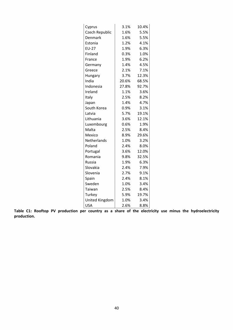
40
Cyprus 3.1% 10.4%
Czech Republic 1.6% 5.5%
Denmark 1.6% 5.5%
Estonia 1.2% 4.1%
EU-27 1.9% 6.3%
Finland 0.3% 1.0%
France 1.9% 6.2%
Germany 1.4% 4.5%
Greece 2.1% 7.1%
Hungary 3.7% 12.3%
India 20.6% 68.5%
Indonesia 27.8% 92.7%
Ireland 1.1% 3.6%
Italy 2.5% 8.2%
Japan 1.4% 4.7%
South Korea 0.9% 3.1%
Latvia 5.7% 19.1%
Lithuania 3.6% 12.1%
Luxembourg 0.6% 1.9%
Malta 2.5% 8.4%
Mexico 8.9% 29.6%
Netherlands 1.0% 3.2%
Poland 2.4% 8.0%
Portugal 3.6% 12.0%
Romania 9.8% 32.5%
Russia 1.9% 6.3%
Slovakia 2.4% 7.9%
Slovenia 2.7% 9.1%
Spain 2.4% 8.1%
Sweden 1.0% 3.4%
Taiwan 2.5% 8.4%
Turkey 5.9% 19.7%
United Kingdom 1.0% 3.4%
USA 2.6% 8.8%
Table C1: Rooftop PV production per country as a share of the electricity use minus the hydroelectricity production.
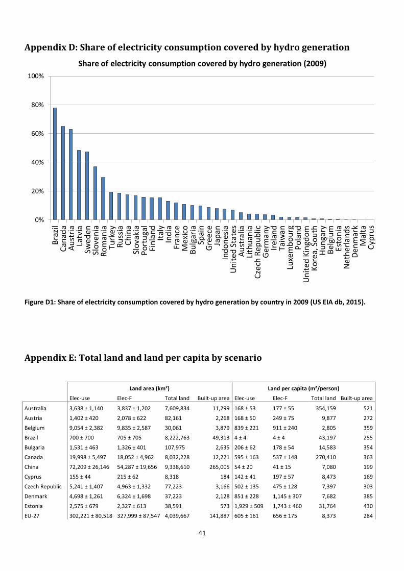
41
Appendix D: Share of electricity consumption covered by hydro generation
0%
20%
40%
60%
80%
100%
Bra
zil
Can
ada
Au
stri
aLa
tvia
Swed
enSl
ove
nia
Ro
man
iaTu
rkey
Ru
ssia
Ch
ina
Slov
akia
Por
tuga
lFi
nla
nd
Ital
yIn
dia
Fran
ceM
exic
oB
ulg
aria
Spai
nG
reec
eJa
pan
Ind
on
esia
Un
ited
Sta
tes
Au
stra
liaLi
thu
ania
Cze
ch R
epu
blic
Ger
ma
nyIr
elan
dTa
iwan
Luxe
mb
ou
rgP
ola
nd
Un
ited
Kin
gdom
Kor
ea, S
ou
thH
unga
ryB
elgi
um
Esto
nia
Net
her
land
sD
enm
ark
Mal
taC
ypru
s
Share of electricity consumption covered by hydro generation (2009)
Figure D1: Share of electricity consumption covered by hydro generation by country in 2009 (US EIA db, 2015).
Appendix E: Total land and land per capita by scenario
Land area (km²) Land per capita (m²/person)
Elec-use Elec-F Total land Built-up area Elec-use Elec-F Total land Built-up area
Australia 3,638 ± 1,140 3,837 ± 1,202 7,609,834 11,299 168 ± 53 177 ± 55 354,159 521
Austria 1,402 ± 420 2,078 ± 622 82,161 2,268 168 ± 50 249 ± 75 9,877 272
Belgium 9,054 ± 2,382 9,835 ± 2,587 30,061 3,879 839 ± 221 911 ± 240 2,805 359
Brazil 700 ± 700 705 ± 705 8,222,763 49,313 4 ± 4 4 ± 4 43,197 255
Bulgaria 1,531 ± 463 1,326 ± 401 107,975 2,635 206 ± 62 178 ± 54 14,583 354
Canada 19,998 ± 5,497 18,052 ± 4,962 8,032,228 12,221 595 ± 163 537 ± 148 270,410 363
China 72,209 ± 26,146 54,287 ± 19,656 9,338,610 265,005 54 ± 20 41 ± 15 7,080 199
Cyprus 155 ± 44 215 ± 62 8,318 184 142 ± 41 197 ± 57 8,473 169
Czech Republic 5,241 ± 1,407 4,963 ± 1,332 77,223 3,166 502 ± 135 475 ± 128 7,397 303
Denmark 4,698 ± 1,261 6,324 ± 1,698 37,223 2,128 851 ± 228 1,145 ± 307 7,682 385
Estonia 2,575 ± 679 2,327 ± 613 38,591 573 1,929 ± 509 1,743 ± 460 31,764 430
EU-27 302,221 ± 80,518 327,999 ± 87,547 4,039,667 141,887 605 ± 161 656 ± 175 8,373 284

42
Finland 38,273 ± 9,689 33,924 ± 8,588 278,053 1,974 7,169 ± 1,815 6,354 ± 1,609 56,922 370
France 26,372 ± 7,147 30,670 ± 8,312 539,687 18,134 408 ± 110 474 ± 128 8,463 280
Germany 52,369 ± 13,894 57,727 ± 15,316 344,330 26,270 639 ± 170 705 ± 187 4,256 321
Greece 2,751 ± 755 3,826 ± 1,050 114,916 2,199 246 ± 67 342 ± 94 11,522 197
Hungary 2,907 ± 853 3,164 ± 929 89,978 4,136 290 ± 85 316 ± 93 9,033 413
India 11,481 ± 7,069 11,454 ± 7,053 2,909,644 206,231 10 ± 6 10 ± 6 2,498 173
Indonesia 1,283 ± 1,136 1,494 ± 1,322 1,705,727 40,029 5 ± 5 6 ± 6 7,628 169
Ireland 4,409 ± 1,155 5,721 ± 1,498 63,581 1,289 972 ± 255 1,261 ± 330 15,189 284
Italy 13,998 ± 3,893 17,063 ± 4,745 283,927 12,887 237 ± 66 289 ± 80 4,977 218
Japan 34,031 ± 9,050 37,145 ± 9,878 338,211 17,741 266 ± 71 290 ± 77 2,847 139
South Korea 14,539 ± 3,786 12,128 ± 3,158 89,621 4,960 296 ± 77 247 ± 64 1,974 101
Latvia 762 ± 244 1,121 ± 359 60,857 873 356 ± 114 524 ± 168 29,033 408
Lithuania 1,351 ± 396 1,656 ± 485 62,217 1,418 427 ± 125 523 ± 153 19,816 448
Luxembourg 659 ± 169 641 ± 164 2,590 137 1,324 ± 339 1,287 ± 330 5,203 276
Malta 65 ± 18 78 ± 22 165 62 157 ± 44 188 ± 52 776 150
Mexico 3,329 ± 1,219 3,575 ± 1,309 1,906,300 19,018 29 ± 10 31 ± 11 16,697 163
Netherlands 16,595 ± 4,328 19,047 ± 4,968 31,687 4,408 1,004 ± 262 1,152 ± 301 2,040 267
Poland 16,923 ± 4,693 17,305 ± 4,799 304,164 11,358 444 ± 123 454 ± 126 8,028 298
Portugal 1,718 ± 502 1,985 ± 580 89,322 2,381 163 ± 48 188 ± 55 8,667 225
Romania 1,732 ± 659 1,902 ± 724 228,614 7,410 85 ± 32 93 ± 36 11,295 364
Russia 91,315 ± 24,777 64,517 ± 17,506 15,964,790 47,848 643 ± 175 455 ± 123 115,404 337
Slovakia 1,779 ± 493 1,874 ± 519 48,063 1,581 330 ± 92 348 ± 96 8,928 293
Slovenia 530 ± 149 554 ± 156 20,072 546 260 ± 73 272 ± 76 9,874 268
Spain 9,383 ± 2,608 10,663 ± 2,964 488,354 8,588 202 ± 56 230 ± 64 10,759 185
Sweden 26,022 ± 6,799 19,808 ± 5,175 383,445 4,805 2,798 ± 731 2,130 ± 557 44,130 517
Taiwan 4,824 ± 1,345 3,227 ± 900 35,410 6,829 209 ± 58 140 ± 39 1,532 295
Turkey 5,746 ± 1,854 5,954 ± 1,921 753,637 13,664 81 ± 26 84 ± 27 10,803 192
United Kingdom 58,967 ± 15,418 72,206 ± 18,879 224,095 16,596 947 ± 248 1,159 ± 303 3,885 266
USA 132,026 ± 37,005 144,969 ± 40,633 8,896,353 130,919 430 ± 121 473 ± 132 29,818 427
Table E1: Land area (km2) and land per capita (m2/person) for each WIOD country for: electricity use, electricity footprint, total land and built-up area. 100% solar electricity mix scenario.
Land area (km²) Land per capita (m²/person)
Elec-use Elec-F Total land
Built-up area Elec-use Elec-F
Total land
Built-up area
Australia 17,499 ± 4,605 20,306 ± 5,343 7,609,834 11,299 807 ± 212 936 ± 246 354,159 521
Austria 19,815 ± 5,023 24,950 ± 6,325 82,161 2,268 2,375 ± 602 2,990 ± 758 9,877 272
Belgium 58,863 ± 14,834 55,133 ± 13,894 30,061 3,879 5,452 ± 1,374 5,107 ± 1,287 2,805 359
Brazil 38,369 ± 10,596 38,739 ± 10,699 8,222,763 49,313 198 ± 55 200 ± 55 43,197 255
Bulgaria 5,375 ± 1,424 5,395 ± 1,429 107,975 2,635 722 ± 191 725 ± 192 14,583 354
Canada 233,732 ± 58,931 221,384 ± 55,817 8,032,228 12,221 6,950 ± 1,752 6,583 ± 1,660 270,410 363
China 513,445 ± 136,455 436,849 ± 116,098 9,338,610 265,005 386 ± 103 328 ± 87 7,080 199
Cyprus 808 ± 208 1,060 ± 272 8,318 184 741 ± 190 972 ± 250 8,473 169
Czech Republic 27,109 ± 6,874 25,594 ± 6,490 77,223 3,166 2,596 ± 658 2,451 ± 621 7,397 303
Denmark 41,584 ± 10,483 37,058 ± 9,342 37,223 2,128 7,529 ± 1,898 6,710 ± 1,691 7,682 385
Estonia 11,469 ± 2,902 11,513 ± 2,914 38,591 573 8,594 ± 2,175 8,627 ± 2,183 31,764 430
EU-27 1,649,098 ± 417,238
1,836,022 ± 464,704 4,039,667 141,887 3,300 ± 835 3,674 ± 930 8,373 284
Finland 172,195 ± 43,169 164,913 ± 41,344 278,053 1,974 32,253 ± 30,889 ± 56,922 370
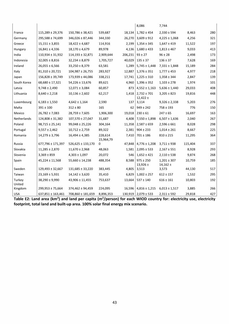
43
8,086 7,744
France 115,289 ± 29,376 150,786 ± 38,421 539,687 18,134 1,782 ± 454 2,330 ± 594 8,463 280
Germany 295,588 ± 74,699 346,026 ± 87,446 344,330 26,270 3,609 ± 912 4,225 ± 1,068 4,256 321
Greece 15,151 ± 3,855 18,422 ± 4,687 114,916 2,199 1,354 ± 345 1,647 ± 419 11,522 197
Hungary 16,841 ± 4,336 18,170 ± 4,679 89,978 4,136 1,680 ± 433 1,813 ± 467 9,033 413
India 110,934 ± 31,932 114,193 ± 32,871 2,909,644 206,231 93 ± 27 96 ± 28 2,498 173
Indonesia 32,005 ± 8,816 32,234 ± 8,879 1,705,727 40,029 135 ± 37 136 ± 37 7,628 169
Ireland 26,055 ± 6,566 33,250 ± 8,379 63,581 1,289 5,745 ± 1,448 7,331 ± 1,848 15,189 284
Italy 81,310 ± 20,721 104,987 ± 26,755 283,927 12,887 1,376 ± 351 1,777 ± 453 4,977 218
Japan 156,828 ± 39,749 173,939 ± 44,086 338,211 17,741 1,225 ± 310 1,358 ± 344 2,847 139
South Korea 68,680 ± 17,321 54,226 ± 13,676 89,621 4,960 1,396 ± 352 1,103 ± 278 1,974 101
Latvia 9,748 ± 2,490 12,071 ± 3,084 60,857 873 4,552 ± 1,163 5,636 ± 1,440 29,033 408
Lithuania 8,640 ± 2,218 10,136 ± 2,602 62,217 1,418 2,732 ± 701 3,205 ± 823 19,816 448
Luxembourg 6,183 ± 1,550 4,642 ± 1,164 2,590 137 12,422 ± 3,114 9,326 ± 2,338 5,203 276
Malta 391 ± 100 312 ± 80 165 62 949 ± 242 758 ± 193 776 150
Mexico 26,782 ± 7,083 28,759 ± 7,605 1,906,300 19,018 230 ± 61 247 ± 65 16,697 163
Netherlands 124,808 ± 31,382 107,570 ± 27,047 31,687 4,408 7,550 ± 1,898 6,507 ± 1,636 2,040 267
Poland 98,715 ± 25,141 99,048 ± 25,226 304,164 11,358 2,587 ± 659 2,596 ± 661 8,028 298
Portugal 9,557 ± 2,462 10,712 ± 2,759 89,322 2,381 904 ± 233 1,014 ± 261 8,667 225
Romania 14,279 ± 3,796 16,494 ± 4,385 228,614 7,410 701 ± 186 810 ± 215 11,295 364
Russia 677,796 ± 171,397 526,625 ± 133,170 15,964,790 47,848 4,776 ± 1,208 3,711 ± 938 115,404 337
Slovakia 11,285 ± 2,870 11,670 ± 2,968 48,063 1,581 2,095 ± 533 2,167 ± 551 8,928 293
Slovenia 3,369 ± 859 4,303 ± 1,097 20,072 546 1,652 ± 421 2,110 ± 538 9,874 268
Spain 45,224 ± 11,568 55,660 ± 14,238 488,354 8,588 975 ± 250 1,201 ± 307 10,759 185
Sweden 129,493 ± 32,667 131,685 ± 33,220 383,445 4,805 13,926 ± 3,513
14,162 ± 3,573 44,130 517
Taiwan 23,169 ± 5,931 14,142 ± 3,620 35,410 6,829 1,002 ± 257 612 ± 157 1,532 295
Turkey 38,290 ± 9,990 43,906 ± 11,455 753,637 13,664 537 ± 140 616 ± 161 10,803 192 United Kingdom 299,953 ± 75,664 374,462 ± 94,459 224,095 16,596 4,816 ± 1,215 6,013 ± 1,517 3,885 266
USA 637,851 ± 163,461 708,860 ± 181,659 8,896,353 130,919 2,079 ± 533 2,311 ± 592 29,818 427
Table E2: Land area (km2) and land per capita (m2/person) for each WIOD country for: electricity use, electricity footprint, total land and built-up area. 100% solar final energy mix scenario.

44
Appendix D: Land availability at country level
Figure D1: Land availability at country level as defined in Section 3.1.
References
Alston, J.M., Beddow, J.M., Pardey, P.G., 2009. Agricultural Research, Productivity, and Food Prices in the Long Run. Science 325, 1209–1210. doi:10.1126/science.1170451
Armaroli, N., Balzani, V., 2011. Towards an electricity-powered world. Energy Environ. Sci. 4, 3193–3222. doi:10.1039/C1EE01249E
Arto, I., Capellán-Pérez, I., Lago, R., Bueno, G., Bermejo, R., 2016. The energy requirements of a developed world. Energy Sustain. Dev. 33, 1–13. doi:10.1016/j.esd.2016.04.001
Arto, I., Genty, A., Rueda-Cantuche, J.M., Villanueva, Andreoni, V., 2012. Global Resources Use and Pollution: Vol. I, Production, Consumption and Trade (1995-2008). Institute for Prospective and Technological Studies, Joint Research Centre.
Baiocchi, G., Minx, J.C., 2010. Understanding changes in the UK’s CO2 emissions: a global perspective. Environ. Sci. Technol. 44, 1177–1184. doi:10.1021/es902662h
Bergamasco, L., Asinari, P., 2011. Scalable methodology for the photovoltaic solar energy potential assessment based on available roof surface area: Application to Piedmont Region (Italy). Sol. Energy 85, 1041–1055. doi:10.1016/j.solener.2011.02.022
Bocca, A., Chiavazzo, E., Macii, A., Asinari, P., 2015. Solar energy potential assessment: An overview and a fast modeling approach with application to Italy. Renew. Sustain. Energy Rev. 49, 291–296. doi:10.1016/j.rser.2015.04.138

45
Breyer, C., Bogdanov, D., Komoto, K., Ehara, T., Song, J., Enebish, N., 2015. North-east Asian super grid: renewable energy mix and economics. Jpn. J. Appl. Phys. 54, 08KJ01.
Briner, G., 2009. The climate change mitigation potential of the solar PV industry: a life cycle perspective. M Sc thesis, Centre for Environmental Policy, Imperial College London, London, UK.
Brower, M., Barton, M., Lledó, L., Dubois, J., 2013. A study of wind speed variability using global reanalysis data. AWS Truepower.
Byrne, J., Taminiau, J., Kurdgelashvili, L., Kim, K.N., 2015. A review of the solar city concept and methods to assess rooftop solar electric potential, with an illustrative application to the city of Seoul. Renew. Sustain. Energy Rev. 41, 830–844. doi:10.1016/j.rser.2014.08.023
Cansino, J.M., Pablo-Romero, M. del P., Román, R., Yñiguez, R., 2011. Taxes incentives to promote res deployment: the Eu-27 case, in: Sustainable Growth and Applications in Renewable Energy Sources. INTECH Open Access Publisher.
Connolly, D., Lund, H., Mathiesen, B.V., Leahy, M., 2011. The first step towards a 100% renewable energy-system for Ireland. Appl. Energy, The 5th Dubrovnik Conference on Sustainable Development of Energy, Water and Environment Systems, held in Dubrovnik September/October 2009 88, 502–507. doi:10.1016/j.apenergy.2010.03.006
Daly, H.E., 2005. Economics In A Full World. Sci. Am. 293, 100–107. doi:10.1038/scientificamerican0905-100 de Castro, C., Carpintero, Ó., Frechoso, F., Mediavilla, M., de Miguel, L.J., 2014. A top-down approach to assess
physical and ecological limits of biofuels. Energy 64, 506–512. doi:10.1016/j.energy.2013.10.049 de Castro, C., Mediavilla, M., Miguel, L.J., Frechoso, F., 2013. Global solar electric potential: A review of their
technical and sustainable limits. Renew. Sustain. Energy Rev. 28, 824–835. doi:10.1016/j.rser.2013.08.040 de Castro, C., Mediavilla, M., Miguel, L.J., Frechoso, F., 2011. Global wind power potential: Physical and technological
limits. Energy Policy 39, 6677–6682. doi:10.1016/j.enpol.2011.06.027 Defaix, P.R., van Sark, W.G.J.H.M., Worrell, E., de Visser, E., 2012. Technical potential for photovoltaics on buildings
in the EU-27. Sol. Energy 86, 2644–2653. doi:10.1016/j.solener.2012.06.007 Deng, Y.Y., Haigh, M., Pouwels, W., Ramaekers, L., Brandsma, R., Schimschar, S., Grözinger, J., de Jager, D., 2015.
Quantifying a realistic, worldwide wind and solar electricity supply. Glob. Environ. Change 31, 239–252. doi:10.1016/j.gloenvcha.2015.01.005
Denholm, P., Kulcinski, G.L., 2004. Life cycle energy requirements and greenhouse gas emissions from large scale energy storage systems. Energy Convers. Manag. 45, 2153–2172. doi:10.1016/j.enconman.2003.10.014
Denholm, P., Margolis, R.M., 2008. Land-use requirements and the per-capita solar footprint for photovoltaic generation in the United States. Energy Policy 36, 3531–3543. doi:10.1016/j.enpol.2008.05.035
DESERTEC, 2003. The DESERTEC project [WWW Document]. URL http://www.desertec.org/ (accessed 10.25.15). Deutsche Bank, 2015. Deutsche Bank Markets Research. Solar 2015 Outlook. Dietzenbacher, E., Los, B., Stehrer, R., Timmer, M., de Vries, G., 2013. The Construction of World Input–Output
Tables in the Wiod Project. Econ. Syst. Res. 25, 71–98. doi:10.1080/09535314.2012.761180 European Commission, 2014. COMMUNICATION FROM THE COMMISSION TO THE EUROPEAN PARLIAMENT, THE
COUNCIL, THE EUROPEAN ECONOMIC AND SOCIAL COMMITTEE AND THE COMMITTEE OF THE REGIONS A policy framework for climate and energy in the period from 2020 to 2030 /* COM/2014/015 final */.
FAO/IIASA, 2011. Global Agro-ecological Zones (GAEZ v3.0). FAO Rome and IIASA Laxemburg, Italy and Austria. FAOSTAT, 2015. Statistics Division of the FAO. Food and Agriculture Organization of the United Nations, Rome (Italy). Farthing, A., Carbajales-Dale, M., Mason, S., Carbajales-Dale, P., Matta, P., 2016. Utility-Scale Solar PV in South
Carolina: Analysis of Suitable Lands and Geographical Potential. Biophys. Econ. Resour. Qual. 1, 8. doi:10.1007/s41247-016-0009-5
François, B., Hingray, B., Raynaud, D., Borga, M., Creutin, J.D., 2016. Increasing climate-related-energy penetration by integrating run-of-the river hydropower to wind/solar mix. Renew. Energy 87, Part 1, 686–696. doi:10.1016/j.renene.2015.10.064
Fthenakis, V., Kim, H.C., 2009. Land use and electricity generation: A life-cycle analysis. Renew. Sustain. Energy Rev. 13, 1465–1474. doi:10.1016/j.rser.2008.09.017
García-Olivares, A., 2016. Energy for a sustainable post-carbon society. Sci. Mar. 80, 257–268. doi:10.3989/scimar.04295.12A
García-Olivares, A., Ballabrera-Poy, J., García-Ladona, E., Turiel, A., 2012. A global renewable mix with proven technologies and common materials. Energy Policy 41, 561–574. doi:10.1016/j.enpol.2011.11.018
46
Grassini, P., Eskridge, K.M., Cassman, K.G., 2013. Distinguishing between yield advances and yield plateaus in historical crop production trends. Nat. Commun. 4, 2918. doi:10.1038/ncomms3918
Greenpeace, GWEC, SolarPowerEurope, 2015. Energy [R] evolution-A sustainable world energy outlook 2015. Greenpeace, GWEC, SolarPowerEurope.
GSE, 2015. Rapporto Statistico “Energia da fonti rinnovabili” Anno 2013. Gestore Servizi Energetici. Gulagi, A., Bogdanov, D., Fasihi, M., Breyer, C., 2017. Can Australia Power the Energy-Hungry Asia with Renewable
Energy? Sustainability 9, 233. doi:10.3390/su9020233 Hagos, D.A., Gebremedhin, A., Zethraeus, B., rn, 2014. Solar Water Heating as a Potential Source for Inland Norway
Energy Mix. J. Renew. Energy 2014, e968320. doi:10.1155/2014/968320 Hall, C.A.S., Lambert, J.G., Balogh, S.B., 2014. EROI of different fuels and the implications for society. Energy Policy
64, 141–152. doi:10.1016/j.enpol.2013.05.049 Hernandez, R.R., Hoffacker, M.K., Murphy-Mariscal, M.L., Wu, G.C., Allen, M.F., 2015. Solar energy development
impacts on land cover change and protected areas. Proc. Natl. Acad. Sci. 201517656. doi:10.1073/pnas.1517656112
Horner, R.M., Clark, C.E., 2013. Characterizing variability and reducing uncertainty in estimates of solar land use energy intensity. Renew. Sustain. Energy Rev. 23, 129–137. doi:10.1016/j.rser.2013.01.014
IEA, 2016a. Energy balances statistics. IEA/OCDE. IEA, 2016b. Global EV Outlook 2016. Beyond one million electric cars. OECD/IEA, Paris. IEA, 2006. Barriers to Technology Diffusion: The Case of Solar Thermal Technologies (No. C/IEA/SLT(2006)9).
International Energy Agency, Paris (France). Instituto de Estadísticas de Andalucía, 2015. Instituto de Estadísticas de Andalucía. Instituto de Estadísticas de
Andalucía. IPCC, 2014. Climate Change 2014: Mitigation of Climate Change. Fifth Assess. Rep. Intergov. Panel Clim. Change. IPCC, 2011. Special Report on Renewable Energy Sources and Climate Change Mitigation. Cambridge University
Press, United Kingdom and New York (USA). ISE, 2014. Photovoltaics Report. Fraunhofer ISE. Izquierdo, S., Montañés, C., Dopazo, C., Fueyo, N., 2011. Roof-top solar energy potential under performance-based
building energy codes: The case of Spain. Sol. Energy 85, 208–213. doi:10.1016/j.solener.2010.11.003 Jacobson, M.Z., Delucchi, M.A., 2011. Providing all global energy with wind, water, and solar power, Part I:
Technologies, energy resources, quantities and areas of infrastructure, and materials. Energy Policy 39, 1154–1169. doi:10.1016/j.enpol.2010.11.040
Jacobson, M.Z., Delucchi, M.A., Bazouin, G., Bauer, Z.A., Heavey, C.C., Fisher, E., Morris, S.B., Piekutowski, D.J., Vencill, T.A., Yeskoo, T.W., 2015. 100% clean and renewable wind, water, and sunlight (WWS) all-sector energy roadmaps for the 50 United States. Energy Environ. Sci. 8, 2093–2117.
Jo, J.H., Otanicar, T.P., 2011. A hierarchical methodology for the mesoscale assessment of building integrated roof solar energy systems. Renew. Energy 36, 2992–3000. doi:10.1016/j.renene.2011.03.038
Johansson, B., 2013. Security aspects of future renewable energy systems–A short overview. Energy 61, 598–605. doi:10.1016/j.energy.2013.09.023
Juffe-Bignoli, D., Burgess, N., Bingham, H., Belle, E., de Lima, M., Deguignet, M., Bertzky, B., Milam, A., Martinez-Lopez, J., Lewis, E., others, 2014. Protected planet report 2014. UNEP-WCMC Camb. UK.
La Gennusa, M., Lascari, G., Rizzo, G., Scaccianoce, G., Sorrentino, G., 2011. A model for predicting the potential diffusion of solar energy systems in complex urban environments. Energy Policy 39, 5335–5343. doi:10.1016/j.enpol.2011.05.031
Laborde, D., 2011. Assessing the land use change consequences of European biofuel policies. Int. Food Policy Inst. IFPRI.
Lenzen, M., 2010. Current State of Development of Electricity-Generating Technologies: A Literature Review. Energies 3, 462–591. doi:10.3390/en3030462
Li, X., Zhong, S., Bian, X., Heilman, W.E., 2010. Climate and climate variability of the wind power resources in the Great Lakes region of the United States. J. Geophys. Res. Atmospheres 115, D18107. doi:10.1029/2009JD013415
Lilliestam, J., Ellenbeck, S., 2011. Energy security and renewable electricity trade—Will Desertec make Europe vulnerable to the “energy weapon”? Energy Policy 39, 3380–3391. doi:10.1016/j.enpol.2011.03.035

47
Lo Piano, S., Mayumi, K., 2016. Toward an integrated assessment of the performance of photovoltaic power stations for electricity generation. Appl. Energy. doi:10.1016/j.apenergy.2016.05.102
Lund, H., Mathiesen, B.V., 2009. Energy system analysis of 100% renewable energy systems—The case of Denmark in years 2030 and 2050. Energy 34, 524–531.
Luque, A., Hegedus, S., 2011. Handbook of photovoltaic science and engineering. John Wiley & Sons, Chichester, West Sussex, United Kingdom.
MacKay, D.J.C., 2013. Solar energy in the context of energy use, energy transportation and energy storage. Philos. Trans. R. Soc. Lond. Math. Phys. Eng. Sci. 371, 20110431. doi:10.1098/rsta.2011.0431
Mainzer, K., Fath, K., McKenna, R., Stengel, J., Fichtner, W., Schultmann, F., 2014. A high-resolution determination of the technical potential for residential-roof-mounted photovoltaic systems in Germany. Sol. Energy 105, 715–731. doi:10.1016/j.solener.2014.04.015
MEA, 2005. Millennium Ecosystem Assessment. Ecosystems and Human Well-being: Scenarios, Global Assessment Reports. Island Press, Washington DC (USA).
Melius, J., Margolis, R., Ong, S., 2013. Estimating Rooftop Suitability for PV: A Review of Methods, Patents, and Validation Techniques. National Renewable Energy Laboratory (NREL), Golden, CO.
Miller, L., Gans, F., Kleidon, A., 2011. Estimating maximum global land surface wind power extractability and associated climatic consequences. Earth Syst Dynam 2, 1–12.
MIT, 2015. The future of solar energy. Energy Initiative Massachusetts Institute of Technology, Cambridge (USA). Moriarty, P., Honnery, D., 2016. Can renewable energy power the future? Energy Policy 93, 3–7.
doi:10.1016/j.enpol.2016.02.051 NABCEP, 2012. Photovoltaic (PV) Installer Resource Guide v.5.3. North American Board of Certified Energy
Practitioners, http://www.nabcep.org/wp-content/uploads/2012/08/NABCEP-PV-Installer-Resource-Guide-August-2012-v.5.3.pdf.
NASA SSE, 2008. NASA Surface meteorology and Solar Energy (SSE) Release 6,0 Data Set (Jan 2008). NASA, https://eosweb.larc.nasa.gov/sse/.
Nonhebel, S., 2003. Land-Use Changes Induced by Increased Use of Renewable Energy Sources, in: Dolman, A.J., Verhagen, A., Rovers, C.A. (Eds.), Global Environmental Change and Land Use. Springer Netherlands, pp. 187–202.
NREL, 2014. Dataset: Solar Resources by Class and Country. National Renewable Energy Laboratory, Golden, CO, USA.
NREL, 2012. Renewable Electricity Futures Study (Entire Report) (4 vols. No. NREL/TP-6A20-52409). National Renewable Energy Laboratory, Golden, CO, USA.
Ong, S., Campbell, C., Denholm, P., Margolis, R., Heath, G., 2013. Land-use requirements for solar power plants in the United States. Gold. CO Natl. Renew. Energy Lab.
Ordóñez, J., Jadraque, E., Alegre, J., Martínez, G., 2010. Analysis of the photovoltaic solar energy capacity of residential rooftops in Andalusia (Spain). Renew. Sustain. Energy Rev. 14, 2122–2130. doi:10.1016/j.rser.2010.01.001
Otto, S.A.C., Gernaat, D.E.H.J., Isaac, M., Lucas, P.L., van Sluisveld, M.A.E., van den Berg, M., van Vliet, J., van Vuuren, D.P., 2015. Impact of fragmented emission reduction regimes on the energy market and on CO2 emissions related to land use: A case study with China and the European Union as first movers. Technol. Forecast. Soc. Change 90, Part A, 220–229. doi:10.1016/j.techfore.2014.01.015
Paidipati, J., Frantzis, L., Sawyer, H., Kurrasch, A., 2008. Rooftop photovoltaics market penetration scenarios. National Renewable Energy Laboratory, Golden, Colorado (USA).
Prieto, P.A., Hall, C.A.S., 2013. Spain’s Photovoltaic Revolution: The Energy Return on Investment, 2013th ed. Springer.
Rao, G.L., Sastri, V.M.K., 1987. Land use and solar energy. Habitat Int. 11, 61–75. doi:10.1016/0197-3975(87)90020-8 Raskin, P., Banuri, T., Gallopín, G., Gutman, P., Hammond, A., Kates, R., Swart, R., 2002. Great Transition: The
Promise and Lure of the Times Ahead. Stockholm Environment Institute. REE, 2016. Series Estadísticas del sistema eléctrico español. Red Eléctrica de España,
http://www.ree.es/es/estadisticas-del-sistema-electrico-espanol/indicadores-nacionales/series-estadisticas. REN21, 2015. Renewables 2015. Global Status Report. REN 21, Paris. Rogner, H.-H., Aguilera, R.F., Bertani, R., Bhattacharya, S.C., Dusseault, M.B., Gagnon, L., Haberl, H., Hoogwijk, M.,
Johnson, A., Rogner, M.L., Wagner, H., Yakushev, V., 2012. Chapter 7 - Energy Resources and Potentials, in:

48
Global Energy Assessment - Toward a Sustainable Future. Cambridge University Press, Cambridge, UK and New York, NY, USA and the International Institute for Applied Systems Analysis, Laxenburg, Austria, pp. 423–512.
Sands, R.D., Jones, C.A., Marshall, E., others, 2014. Global drivers of agricultural demand and supply. Econ. Res. Rep. 174.
Scheidel, A., Sorman, A.H., 2012. Energy transitions and the global land rush: Ultimate drivers and persistent consequences. Glob. Environ. Change, Global transformations, social metabolism and the dynamics of socio-environmental conflicts 22, 588–595. doi:10.1016/j.gloenvcha.2011.12.005
Schneider, A., Friedl, M.A., Potere, D., 2009. A new map of global urban extent from MODIS satellite data. Environ. Res. Lett. 4, 044003. doi:10.1088/1748-9326/4/4/044003
Smil, V., 2015. Power Density: A Key to Understanding Energy Sources and Uses. The MIT Press, Cambridge, Massachusetts.
Smil, V., 2010. Energy Transitions: History, Requirements, Prospects. Praeger, Santa Barbara, California, USA. Smil, V., 2008. Energy in nature and society: general energetics of complex systems. MIT Press, Cambridge,
Massachusetts, USA. Smil, V., 1984. Views: On Energy and Land: Switching from fossil fuels to renewable energy will change our patterns
of land use. Am. Sci. 72, 15–21. Smith, P., Gregory, P.J., Vuuren, D. van, Obersteiner, M., Havlík, P., Rounsevell, M., Woods, J., Stehfest, E., Bellarby,
J., 2010. Competition for land. Philos. Trans. R. Soc. B Biol. Sci. 365, 2941–2957. doi:10.1098/rstb.2010.0127 Sorensen, B., 1999. Long-term scenarios for global energy demand and supply: four global greenhouse mitigation
scenarios (No. 359). Roskilde Universitet, Roskilde, Denmark. Soulé, M.E., Sanjayan, M.A., 1998. ECOLOGY: Conservation Targets: Do They Help? Science 279, 2060–2061.
doi:10.1126/science.279.5359.2060 Squatrito, R., Sgroi, F., Tudisca, S., Trapani, A.M.D., Testa, R., 2014. Post feed-in scheme photovoltaic system
feasibility evaluation in Italy: Sicilian case studies. Energies 7, 7147–7165. Šúri, M., Huld, T.A., Dunlop, E.D., Ossenbrink, H.A., 2007. Potential of solar electricity generation in the European
Union member states and candidate countries. Sol. Energy 81, 1295–1305. doi:10.1016/j.solener.2006.12.007
Trainer, T., 2013a. Can Europe run on renewable energy? A negative case. Energy Policy 63, 845–850. doi:10.1016/j.enpol.2013.09.027
Trainer, T., 2013b. Can the world run on renewable energy? A revised negative case. Humanomics 29, 88–104. doi:10.1108/08288661311319166
Trainer, T., 2012. A critique of Jacobson and Delucchi’s proposals for a world renewable energy supply. Energy Policy 44, 476–481. doi:10.1016/j.enpol.2011.09.037
Trainer, T., 2010. Can renewables etc. solve the greenhouse problem? The negative case. Energy Policy 38, 4107–4114. doi:10.1016/j.enpol.2010.03.037
Turner, J.A., 1999. A Realizable Renewable Energy Future. Science 285, 687–689. doi:10.1126/science.285.5428.687 UN, 2015. World Population Prospects: The 2015 Revision. United Nations, Department of Economic and Social
Affairs Population Division. ST/ESA/SER.A/313. UN Comtrade, 2015. UN Comtrade Database. US ACT, 2007. Energy Independence and Security Act of 2007 (No. PUBLIC LAW 110–140—DEC. 19, 2007). US EIA db, 2015. International Energy Statistics (Database). US Energy Information Administration,
http://www.eia.gov/cfapps/ipdbproject/IEDIndex3.cfm. Vačkář, D., 2012. Ecological Footprint, environmental performance and biodiversity: A cross-national comparison.
Ecol. Indic., The State of the Art in Ecological Footprint: Theory and Applications 16, 40–46. doi:10.1016/j.ecolind.2011.08.008
Valin, H., Peters, D., van den Berg, M., Frank, S., Havlik, P., Forsell, N., Hamelinck, C., Pirker, J., Mosnier, A., Balkovic, J., others, 2015. The land use change impact of biofuels consumed in the EU: Quantification of area and greenhouse gas impacts.
Wackernagel, M., Schulz, N.B., Deumling, D., Linares, A.C., Jenkins, M., Kapos, V., Monfreda, C., Loh, J., Myers, N., Norgaard, R., Randers, J., 2002. Tracking the ecological overshoot of the human economy. Proc. Natl. Acad. Sci. 99, 9266–9271. doi:10.1073/pnas.142033699

49
Wagner, F., 2014. Considerations for an EU-wide use of renewable energies for electricity generation. Eur. Phys. J. Plus 129, 1–14. doi:10.1140/epjp/i2014-14219-7
Ward, D.J., Inderwildi, O.R., 2012. Global and local impacts of UK renewable energy policy. Energy Environ. Sci. 6, 18–24. doi:10.1039/C2EE22342B
WCED, 1987. Our common future (Report of the World Commission on Environment and Development). United Nations.
Weber, C.L., 2009. Measuring structural change and energy use: Decomposition of the US economy from 1997 to 2002. Energy Policy 37, 1561–1570. doi:10.1016/j.enpol.2008.12.027
Weitemeyer, S., Kleinhans, D., Vogt, T., Agert, C., 2015. Integration of Renewable Energy Sources in future power systems: The role of storage. Renew. Energy 75, 14–20. doi:10.1016/j.renene.2014.09.028
WEO, 2014. World Energy Outlook 2014. OECD / IEA, Paris. Wiginton, L.K., Nguyen, H.T., Pearce, J.M., 2010. Quantifying rooftop solar photovoltaic potential for regional
renewable energy policy. Comput. Environ. Urban Syst., Geospatial Cyberinfrastructure 34, 345–357. doi:10.1016/j.compenvurbsys.2010.01.001
Wirth, H., 2015. Recent facts about photovoltaics in Germany. Fraunhofer Institute for Solar Energy Systems, Germany.
WWF, 2011. The energy report: 100% renewable energy by 2050. WWF, Ecofys, OMA.