assessing thermal comfort and performance of the airfloor ......to enhance air quality and radiant...

CIBSE Technical Symposium, London, UK 12-13 April 2018

of 31

Assessing Thermal Comfort and Performance of the Airfloor HVAC System using Multi-Software Coupled Modelling Method JIANNAN LUO BENG(HONS), MSC (EDE), CENG, MCIBSE, LEED AP (BD+C), WELL AP, BREEAM INTL. ASSESSOR Environmental Engineering, Foster + Partners [email protected] DR. NIALL O’SULLIVAN BENG(HONS), PG DIP, MENG(HONS), PH.D., MINSTP, LEED AP Environmental Engineering, Foster + Partners [email protected] ANDREW JACKSON MENG(HONS), CENG, MCIBSE, MASHRAE Environmental Engineering, Foster + Partners [email protected]

Abstract Underfloor Air Distribution (UFAD) is recognised in the HVAC industry as a potentially energy-efficient system type exhibiting both enhanced air quality and radiant thermal comfort. The importance of these criteria is addressed in the WELL building standard. The Airfloor system is a variation of the UFAD system, and was identified as lacking validated modelling methodology to demonstrate its dynamic thermal performance. An innovative multi-software coupled modelling method is presented in this paper, using IES-VE and OpenFOAM CFD. This study demonstrates an analytical model, which is applied to assess of the peak and part load thermal performance of a case study building utilising this novel UFAD system. The results show that, 14% more annual comfort hours (under ASHRAE 55-2013), with 6% reduced energy consumption can be achieved, comparing to a typical displacement ventilation system (without the floor plenum).

Keywords HVAC; Underfloor Air Distribution (UFAD); Computational Fluid

Dynamics (CFD); Dynamic Simulation Modelling (DSM); Thermal Comfort

1.0 Introduction

Underfloor Air Distribution (UFAD) is often considered as an energy-efficient method to enhance air quality and radiant thermal comfort, improving occupants’ health and comfort (1). The Airfloor system is a variation of the typical UFAD system, and works by ‘supplying air to a network of hollow steel forms embedded in a concrete slab which operates as an efficient air plenum and heat-storage mass’ (1). Although this system performs similarly to the traditional UFAD system, there are some differences between the two systems. To date, limited research has been conducted to assess the thermal performance of the system. The existence of thermal mass and heat transfer between different areas/zones of the air plenum to the upper/lower floor surfaces make it a dynamic problem to solve.


of 31

This study aims to provide an analytical method using OpenFOAM (Computational Fluid Dynamics) and IES-Virtual Environment (Dynamic Simulation Modelling) to assess the performance of this novel UFAD system within a case study building (Fortaleza Hall, Racine). This is to provide a viable solution not only to demonstrate the steady-state thermal behaviour of the system, but also provide a dynamic thermal model with CFD-validated HVAC air-side schematic to help understand the annual performance of the system, and assist further engineering studies such as part load assessment and thermal comfort prediction.

In this paper, a literature review will firstly be given to understand the current research available for the UFAD systems, and to understand any limitations of these existing studies. Secondly, the analytical and simulation methodology will be demonstrated, within the research boundaries and limitations identified in this paper. Lastly, the thermal behaviour of this novel UFAD system will be presented and discussed, in both peak summer and winter conditions. In addition, the annual dynamic thermal performance of such system and its advantages will be analysed and discussed.

2.0 Literature Review

2.1 Past Research on the Underfloor Air Distribution (UFAD) System

The UFAD system features a supply air plenum located underneath the occupied floor, see Figure 1. The air will be either ducted to the terminal diffusers, or supplied through the open plenum space; offering efficient air supply, and allowing architectural flexibility (2). This type of system typically uses centralised diffusers (such as swirl diffusers) and/or perimeter diffusers (such as linear grilles) to distribute the conditioned air (3). By using this supply method, the low-level supply and high-level return can create a stratification effect, especially in summer, and improve ventilation effectiveness (4). Meanwhile, the air plenum has conductive and radiative heat transfer with the upper occupied floor, reducing the room’s cooling and heating load, while providing radiant thermal comfort for the occupants (5).

Figure 1 – Illustration of a typical UFAD system


of 31

Centre for the Built Environment (CBE) of UC Berkeley developed a simplified UFAD design tool to estimate the required supply flow rate, based on the internal cooling load split (6). This provides a user-friendly interface for sizing the UFAD system and estimating the stratification behaviour. Based on a detailed study, American Society of Heating, Refrigerating and Air-Conditioning Engineers (ASHRAE) also provided a thorough design guide to support and improve the UFAD design (7).

Various types of commercial UFAD systems and bespoke designs were developed, and validations/tests/simulations were provided for some of them. Linden et al (8) provided a comparative study between the UFAD system and the traditional overhead (OH) system in 3 U.S. climate zones, using a generic 3-storey office building. They found that the UFAD system was achieving more energy savings and had lower peak cooling coil load compared to the OH system. Park (9) presented a transient multi-dimensional numerical solution for the hollow core system and validated using EnergyPlus and experimental data. He also considered various design factors which might affect the system performance such as supply air temperatures, hollow core depth, core diameters, etc. While Webster et al (10) integrated the CFD and mock-up test results into the EnergyPlus and created a new model to simulate the performance of the UFAD system.

2.2 Introduction to the Airfloor system and past research

Airfloor system is a variation of the UFAD system. It forces the conditioned air being supplied to the middle of the room through the ventilation duct and splash box, travelling through a network of hollow steel forms underneath the concrete slab and terrazzo finish, and finally being supplied through the perimeter grilles (1). The appearance of the system and its operating mechanism is showing in Figure 2.

Figure 2 – Appearance and operating mechanism of the Airfloor system (image

source: Airfloor Inc.)


of 31

This novel system has a different air supply methodology than the traditional UFAD system. Normal UFAD systems supply the conditioned air through the perimeter duct into the underfloor plenum and then reject air through the centre-located swirl diffusers or perimeter diffusers (2). Whereas this novel UFAD system supplies the conditioned air directly to the centre of the room; this creates the strongest radiant effect at the centre, with the air then exiting the floor via the perimeter grilles to deal with the perimeter load; as shown below in Figure 3.

Figure 3 – Differences in air transfer routes between the novel (left) and traditional UFAD system (right) Chapman (11) provided a simple psychrometry study summarising the fundamentals of how the system controls the operative temperature while maintaining the room relative humidity condition at the desired level under ASHRAE 55 standard (12). Chapman (13) also carried out a steady-state calculation to understand the temperature loss from the system to the cold ambient under different insulation thickness, to better size the system.

2.3 Limitations and Knowledge Gaps

To date, there has been limited researches done for this novel UFAD system, mainly due to the complexity of the hollow core geometry and lack of completed projects using such a system.

There are some validated model and simulation approaches developed for the traditional UFAD system, however those air plenum geometries and supply strategies are different from the novel one. For instance, the hollow core system simulated by Park (9) has a 1-D axial direction supply, whereas the novel UFAD system normally has multiple flow directions. Also, most of the annual simulations carried out for the UFAD system concentrated on the energy performance and peak load reduction (3). There were limited studies addressed the performance optimisation under part load conditions, for instance, controlling relative humidity by re-heating.

Therefore, this paper aims to provide a multi-software coupled method, to be able to simulate this novel UFAD system’s peak load thermal comfort performance, and in the meantime, be able to simulate the part load hourly performance, offering future suggestions on effectively operating the system and keep improving building’s thermal performance.


of 31

3.0 Methodology

3.1 Introduction to the Case Study Building

3.1.1 Background Information

To assess the system within a more practical context, a case study building was selected. SC Johnson’s Fortaleza Hall is located at Racine, Wisconsin, designed by Foster + Partners and completed in 2010. The building utilises this novel UFAD system in the main hall area, together with other energy efficient measures, and achieved the LEED Gold certification in 2011 (14). As shown in Figure 4, the building consists of the main hall, legacy gallery, main entrance, mezzanine café and community building. The main interest zone of the building and the research boundary were within the main hall and connected adjacent areas (such as legacy gallery, mezzanine café, main entrance). The other zones such as community building and upper-level canteen were excluded. They are considered to be either adiabatic surfaces, or as a pressure outlet condition in the analysis.

Figure 4 – Exterior view (top) and the functional areas (bottom) of the SC Johnson’s Fortaleza Hall (Photographer: Gillfoto)


of 31

3.1.2 Design Conditions and the HVAC System Overview

Multiple independently controlled HVAC systems are providing the air-conditioning to the main hall and surrounding areas, as shown in Figure 5.

Figure 5 – Overview of the HVAC strategies

The occupied space of the main hall and legacy gallery are conditioned by the novel UFAD system, while along the glass-line, there is an independent trench supply mainly to boost the winter heating performance and help to offset the heat loss through the glass. The trench supply can also provide cooling during summer mainly to reduce the perimeter load and prevent excessive stratification which might affect the café area. Another two trench diffusers provide conditioning to the entrance which mainly deals with the infiltration load and heat loss/gain near the glass. The café area is conditioned using a standard displacement ventilation system. Two return locations are within the main roof void, and east hall corridors. A summary of HVAC system capacities is provided in Table 1.


of 31

No. Location Peak Flow Rate Supply Temp. Range

1 Main Hall and Legacy

Gallery UFAD System

22,000 CFM

(10,383 L/s)

53.6-86.0 °F

12.0-30.0 °C

2 Trench Supply 34,000 CFM

(16,046 L/s)

63.0-90.0 °F

17.2-32.2 °C

3 Entrance Trench Supply 2,600 CFM

(1,227 L/s)

63.0-86.0 °F

17.2-30.0 °C

4 Café DV system 3,960 CFM

(1,869 L/s)

63.0-86.0 °F

17.2-30.0 °C

5 East Corridor Return -22,000 CFM

(-10,383 L/s)

n/a

6 Roof Return -30,000 CFM

(-14,158 L/s)

n/a

Table 1 – HVAC design capacities

The build-up and floor supply plenum connections are shown in Figure 6 & 7. Conditioned air is supplied through 6 splash boxes (4 within the main hall, and 2 within the legacy gallery). Then the air is distributed across the whole floor and supplied to the perimeter linear grilles. The thermal properties of the architectural elements are summarised in Table 2.

Figure 6 – The novel UFAD system plenum connection


of 31

Figure 7 – Floor plenum and build-up details

Opaque Material Location U-Value (W/m2K)

External Wall All Building 0.45

Internal Floor/ceiling All Building 1.30

Ground Floor All Building 0.43

Internal Wall All Building 0.56

Roof All Building 0.43

UFAD Top Layer Above UFAD system 3.86

Glazing Material Location U-value

(W/m2K)

G-value

Façade Glazing Main hall & entrance 5.73 0.83

Skylight Glazing Main hall & entrance 1.65 0.30

Table 2 – Thermal properties of the constructions

The internal design load, operating conditions and annual operating profile assumed in the simulation are provided in Table 3 and Figure 8.


of 31

Design Parameter Basis of Design

Occupancy (hall) 100 ft²/person (9.29 m²/person)

Occupancy (café) 25 ft²/person (2.32 m²/person)

Lighting 1.5 W/ft² (16.15 W/m²)

Café small power 1.0 W/ft² (10.76 W/m²)

Infiltration 0.10 ACH across all areas

Main hall setpoint 70.0-80.0 °F (21.1-26.7 °C) (±1°K) / 50% RH% (±5%)

Others setpoint 70.0-75.0 °F (21.1-23.9 °C) (±1°K)

Note: 50% small power load, 30% occupancy load and 60% of the lighting load

were applied to the stratified zones, to capture the thermal plume effect.

Table 3 – Internal design load and design conditions

Figure 8 – Annual operating profiles of the internal loads

3.2 Multi-software Coupled Simulation Method

3.2.1 Overview and the Workflow

To develop a reliable air flow and heat transfer model, two software packages were used in this research:

OpenFOAM is an open source CFD software developed since 2004 (15). It has a wide range of validated numerical models and solvers to help solve the complex fluid flow and heat transfer problems (15). OpenFOAM v2.4.0 was used in this research to develop the flow regimes within the floor plenum, validate heat transfer rate obtained from the Dynamic Simulation Modelling (DSM) software, and assess the temperature distribution within the whole case study building.

0

0.2

0.4

0.6

0.8

1

0 2 4 6 8 10 12 14 16 18 20 22 24

Div

ers

ity F

ac

tor

Hour

Lighting

Occupancy / SmallPower


of 31

IES-VE is a commercial DSM software capable of performing whole building annual dynamic simulation. It can simulate a building’s annual energy consumption, while also providing detailed HVAC and room surface outputs (16). IES-VE v2017.0.2.0 was used in this study to model the complex HVAC systems within the space. The HVAC simulation outputs and surface heat flux/temperatures were used as the boundary condition input into the OpenFOAM CFD model.

Using a well-developed workflow, OpenFOAM and IES-VE provide necessary information for each other to carry out the coupled simulation, while also cross-validating the results at each step to ensure that each part of the simulation remains consistent. The workflow is summarised below:

Figure 9 – Overview of the research workflow

As shown in Figure 9, the methodology can be summarised into following 5 steps:


of 31

Step 1 – Initial Flow Development:

Firstly, the 3.74-inch (0.095 m) floor plenum was built for the CFD simulation. A velocity field was generated using the OpenFOAM software. Then, by post-processing the results, the whole floor plenum was divided into 72 ‘flow-zones’, and the airflow entering/leaving each flow-zone was calculated, see Figure 10.

Figure 10 – Overview of the floor ‘flow-zones’

Step 2 – Develop the HVAC air-side schematic and perform an annual simulation:

Identical 72 flow-zones were also built in IES-VE. By using the flowrates generated in step 1, the airflow could be replicated and simulated in IES-VE. Then, the heat transfer between the floor and upper occupied space could be simulated dynamically to capture the thermal decay effect within the floor. The effect of environmental factors on the floor, such as solar radiation, were also captured by using IES-VE. The hourly surface thermal outputs and system temperature variations were expected to be outputted from IES-VE through this step.

Step 3 – Validate the temperature distribution within the floor under peak conditions:

The peak cooling and heating period was identified via step 2, and heat fluxes from the floor plenum to the lower ground and upper occupied space were generated,


of 31

respectively. The inlet supply temperatures to the splash boxes under the peak period were also applied as the boundary conditions to the floor-level CFD model. Then, the temperature distribution was simulated.

To validate the results, the outlet flow rates obtained from this step were firstly compared against the flow rates from step 1. This was to investigate whether plenum temperature would affect the flow regimes. Then, the outlet temperatures from the CFD were compared against the ones from IES-VE, to seek temperature agreement between both software packages.

Step 4 – Perform overall CFD simulation for the whole building under peak conditions:

Once the temperature and flow rate were both validated from step 3, the overall CFD simulation for the whole case study building was carried out, using the surface temperatures as boundary conditions, and the volumetric internal/infiltration loads taken from the IES-VE. This is to demonstrate the stratification effect and thermal comfort within the case study building.

Step 5 – Carry out an annual simulation based on the validated DSM model:

After validating the IES-VE from models in steps 1-4, a wide range of annual simulation and studies could be carried out by using the node-based flow model to investigate the building’s part load performance, and seeking opportunities to improve the building’s operating performance. This is mainly regarding:

- Thermal decay effect and annual radiant thermal comfort

- Comparison between the novel UFAD system and traditional displacement ventilation system

- Humidity control and re-heating coil demand

3.2.2 IES-VE Set-up and Assumptions

Modules selected:

IES-VE 2017 features many in-software modules which provide different simulation capabilities. In this research, the following analysis modules were used:

- ModelIT (to build building and context geometry)

- Suncast (to simulate shading and self-shading effect)

- ApacheSim (to set up room conditions and internal loads, and perform node-based annual dynamic simulation)

- ApacheHVAC (to set up HVAC system details and BMS control strategies and simulate forced convective heat transfer within the floor plenum)

- MacroFlo (to activate zonal natural flow transfer, and capture buoyancy and stratification effects)


of 31

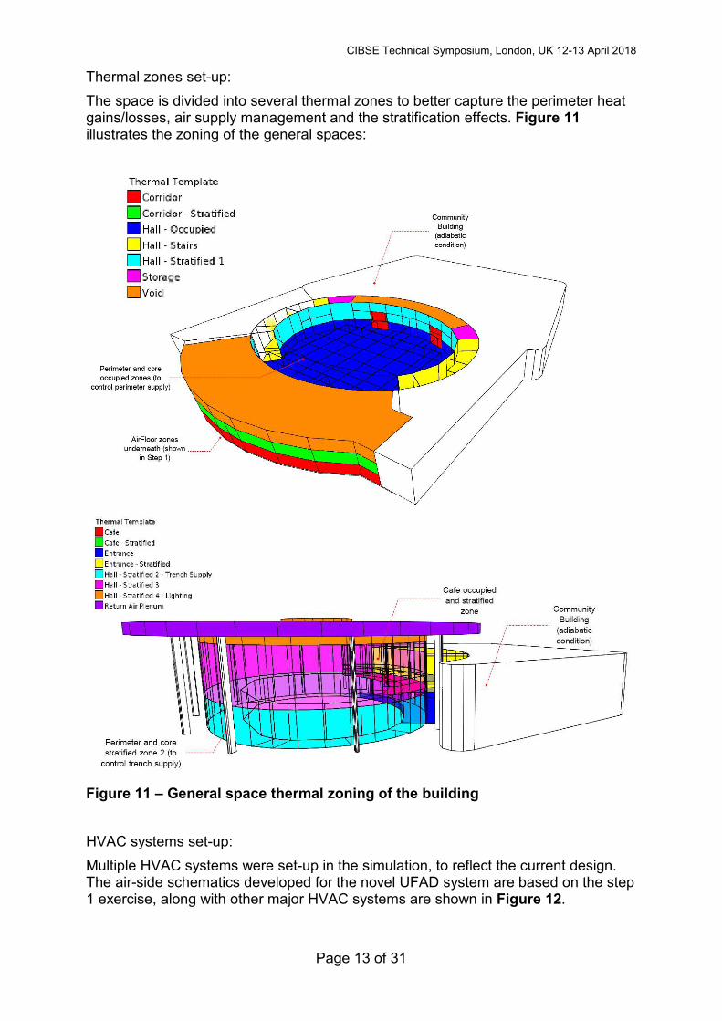
Thermal zones set-up:

The space is divided into several thermal zones to better capture the perimeter heat gains/losses, air supply management and the stratification effects. Figure 11 illustrates the zoning of the general spaces:

Figure 11 – General space thermal zoning of the building

HVAC systems set-up:

Multiple HVAC systems were set-up in the simulation, to reflect the current design. The air-side schematics developed for the novel UFAD system are based on the step 1 exercise, along with other major HVAC systems are shown in Figure 12.


of 31

Figure 12 – HVAC air-side schematic diagram for the HVAC systems

As shown above, the HVAC air-side links and AHUs are controlled by several BMS controllers, a summary of BMS control strategies are listed below in Table 4.

BMS Controller Control Target

Temperature and

RH% controllers

Proportional and ON/OFF control based on CAV

operation, adjust off-coil and re-heat temperature range

(stated in Table 1), to reach the desired indoor

temperature and humidity targets (stated in Table 3)

AHU flow

controllers

Constant flow supply (flow rates stated in Table 1), 1 hour

before and after occupied hours (10:00-21:00), no setback

Minimum outdoor

air ventilation rates

4,400 CFM (2,077 L/s) (main hall and legacy gallery)

3,400 CFM (1,605 L/s) (perimeter glass trench supply)

100% O.A. (dining space and entrance)

Air-side economizer 70.0 °F (21.1°C) temperature high-limit shut-off

Specific fan power UFAD – 1.9 W/(L/s)

*No energy analysis needed for other systems

Fan coil units Only actives when legacy gallery need temperature boost

Table 4 – BMS control targets and strategies


of 31

3.2.3 OpenFOAM CFD Set-up and Assumptions

Mesh set-up:

Figure 13 – 3D CAD model representation of the novel UFAD system and Fortaleza Hall and HVAC inlets/outlets

Figure 13 shows the CAD models were generated using the 3D solid modelling software Rhinoceros 3D for the floor plenum and overall building, respectively. The unstructured mesh grid was generated using the OpenFOAM snappyHexMesh utility, which generates a graded 3D mesh containing hexahedra (hex) and split-hexahedra (split-hex) cells (17). For these simulations, the overall number of cells were 21 million for the floor plenum mesh and 26 million full building mesh (Figure 14) with a smallest cell size of 0.02 m and 0.2 m respectively.

Figure 14 – 3D mesh of the novel UFAD system and Fortaleza Hall with HVAC inlets/outlets

A mesh independency study was also conducted with 20, 40, and 80 control volumes in each direction. This was done equally for all directions, since a 3D representation of the flow of equal resolution is required for comparisons of the calculated values of velocity and pressure at different locations. It was found that for 40 to 80 control volumes, there was less than 1% difference in the results. Therefore, it was concluded that 40 mesh control volumes would be used for computational efficiency. It was also found that the non-dimensional distance (i.e. the distance y to the wall required for flow stability, made dimensionless with by friction velocity and kinematic viscosity) from the wall on all surfaces within the domain ranged from y+ = 0.6–0.9, for the critical range of wall bounded internal flow stability.


of 31

Solver set-up:

The finite volume CFD code OpenFOAM was used to simulate the turbulent velocity and temperature fields. OpenFOAM is a C++ library used primarily to create executables known as applications. The applications fall into two categories: solvers, designed to solve a specific problem in continuum mechanics, and utilities, designed to perform tasks that involve data manipulation (17).

The RANS OpenFOAM solver BuoyantBoussinesqSimpleFoam was used for a steady state, buoyant and incompressible fluid. The SIMPLE (Semi-Implicit method for Pressure linked equations) algorithm is an iterative procedure for time averaged equations (18). In the implementation of the RANS solver, we used the realizable k-ε turbulent closure model for its proven reliability at predicting high Reynolds number flows all the way down to the viscous sub-layer (19). The simulations were carried out for 3000 iterations to reach a statistical convergence criterion of 10−5.

The system simulations, in both winter and summer had fluid properties of density, viscosity, specific heat capacity and temperature defined based upon the specific fluids ambient temperature at sea-level. Internal boundary conditions for these simulations are outlined in Section 3.2.1 (step 3). Inflow conditions were defined using volume flow rate inlets and plenum exhaust was implemented using total pressure outlet conditions with a back-flow temperature defined by the ambient air to solve the thermal gradient at exhaust. Infiltration gain in both cases were applied as a global volume heat flux within the floor plenum, to simulate the plenum leakage rate.

The Fortaleza Hall simulations, in both winter and summer also had fluid properties of density, viscosity, specific heat capacity and temperature defined based upon the specific fluids ambient temperature at sea-level. Internal boundary conditions for these simulations are outlined in Section 3.2.1 (step 4). Occupant and small power gain were applied within the occupied level of 1.5m from the floor on each level. Infiltration was applied in kind as a global heat flux per the whole mesh volume. Inflow conditions were defined at the simplified plenum exhaust, floor grills and extract points as surface normal inlet boundaries as per their operational areas, flow rates and supply/extract temperatures. All back of house areas were applied as total pressure outlet conditions with an average temperature back-flow from their specific zone.

4.0 Results and Discussion

4.1 Development of the Flow Regimes and Air-node Model

4.1.1 Floor Plenum Flow Regimes

Figure 15 shows the velocity field within half of the floor plenum (symmetry boundary applied), clipped at mid-height of the plenum (0.057m).


of 31

Figure 15 – Half-floor plenum velocity field plot

It is observed that the velocity distribution is generally well-organised, with outlet velocities in the range of 0.5-2.2 m/s, which is within the comfort criteria of maximum 4 m/s, as specified by Price Industries (2). There are stagnation zones observed in some areas, which might affect the temperature distribution.

Data sample surfaces were placed at the boundary of each ‘flow-zone’, with over 5000 sample points at each boundary, and the air flow rates entering/leaving each flow-zone were plotted in Figure 16.

Figure 16 – Half-floor air flow rate schematic diagram

The flow rates showing above were applied to the IES-VE HVAC model via individual flow controllers (shown in Figure 12), to capture this complicated air flow transfer.


of 31

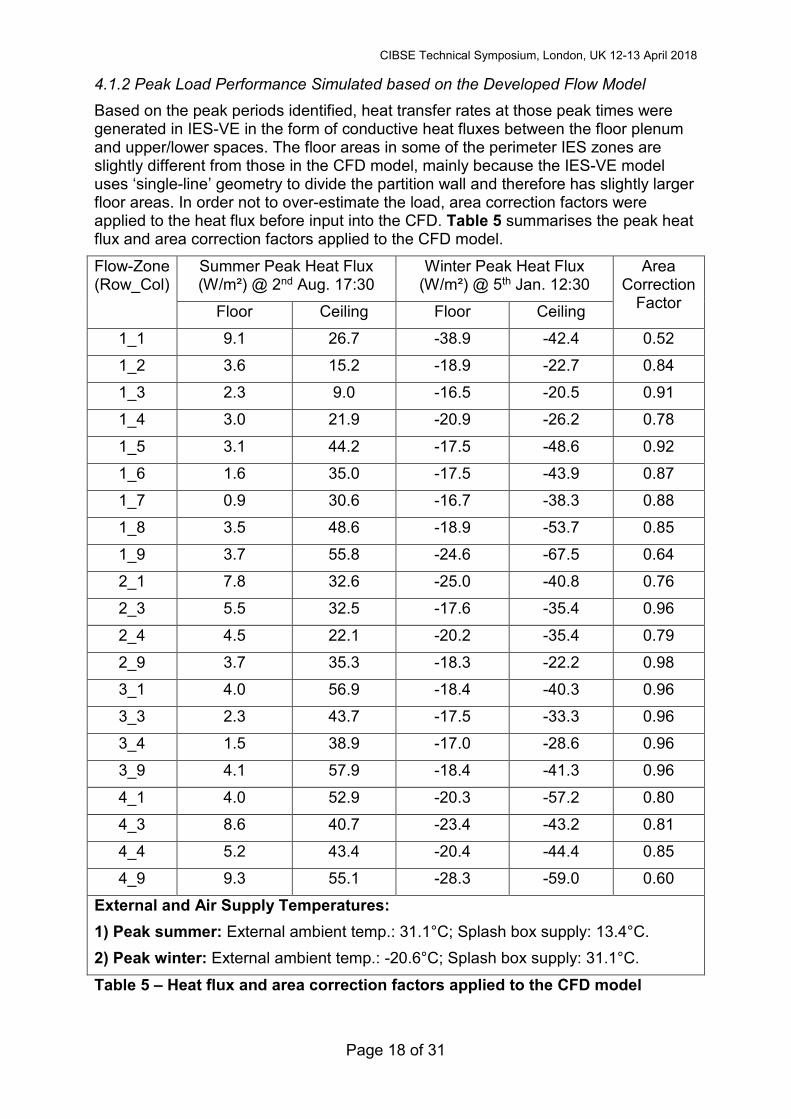
4.1.2 Peak Load Performance Simulated based on the Developed Flow Model

Based on the peak periods identified, heat transfer rates at those peak times were generated in IES-VE in the form of conductive heat fluxes between the floor plenum and upper/lower spaces. The floor areas in some of the perimeter IES zones are slightly different from those in the CFD model, mainly because the IES-VE model uses ‘single-line’ geometry to divide the partition wall and therefore has slightly larger floor areas. In order not to over-estimate the load, area correction factors were applied to the heat flux before input into the CFD. Table 5 summarises the peak heat flux and area correction factors applied to the CFD model.

Flow-Zone (Row_Col)

Summer Peak Heat Flux (W/m²) @ 2nd Aug. 17:30

Winter Peak Heat Flux (W/m²) @ 5th Jan. 12:30

Area Correction

Factor Floor Ceiling Floor Ceiling

1_1 9.1 26.7 -38.9 -42.4 0.52

1_2 3.6 15.2 -18.9 -22.7 0.84

1_3 2.3 9.0 -16.5 -20.5 0.91

1_4 3.0 21.9 -20.9 -26.2 0.78

1_5 3.1 44.2 -17.5 -48.6 0.92

1_6 1.6 35.0 -17.5 -43.9 0.87

1_7 0.9 30.6 -16.7 -38.3 0.88

1_8 3.5 48.6 -18.9 -53.7 0.85

1_9 3.7 55.8 -24.6 -67.5 0.64

2_1 7.8 32.6 -25.0 -40.8 0.76

2_3 5.5 32.5 -17.6 -35.4 0.96

2_4 4.5 22.1 -20.2 -35.4 0.79

2_9 3.7 35.3 -18.3 -22.2 0.98

3_1 4.0 56.9 -18.4 -40.3 0.96

3_3 2.3 43.7 -17.5 -33.3 0.96

3_4 1.5 38.9 -17.0 -28.6 0.96

3_9 4.1 57.9 -18.4 -41.3 0.96

4_1 4.0 52.9 -20.3 -57.2 0.80

4_3 8.6 40.7 -23.4 -43.2 0.81

4_4 5.2 43.4 -20.4 -44.4 0.85

4_9 9.3 55.1 -28.3 -59.0 0.60

External and Air Supply Temperatures:

1) Peak summer: External ambient temp.: 31.1°C; Splash box supply: 13.4°C.

2) Peak winter: External ambient temp.: -20.6°C; Splash box supply: 31.1°C.

Table 5 – Heat flux and area correction factors applied to the CFD model


of 31

4.1.3 Temperature and Flow Validation between CFD and IES-VE Models

After applying the heat flux to the floor plenum CFD model, the updated velocity and temperature field were generated.

Velocity and flow rate validation:

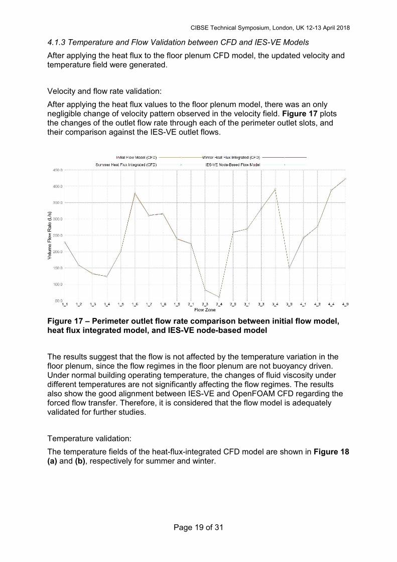
After applying the heat flux values to the floor plenum model, there was an only negligible change of velocity pattern observed in the velocity field. Figure 17 plots the changes of the outlet flow rate through each of the perimeter outlet slots, and their comparison against the IES-VE outlet flows.

Figure 17 – Perimeter outlet flow rate comparison between initial flow model, heat flux integrated model, and IES-VE node-based model

The results suggest that the flow is not affected by the temperature variation in the floor plenum, since the flow regimes in the floor plenum are not buoyancy driven. Under normal building operating temperature, the changes of fluid viscosity under different temperatures are not significantly affecting the flow regimes. The results also show the good alignment between IES-VE and OpenFOAM CFD regarding the forced flow transfer. Therefore, it is considered that the flow model is adequately validated for further studies.

Temperature validation:

The temperature fields of the heat-flux-integrated CFD model are shown in Figure 18 (a) and (b), respectively for summer and winter.


of 31

(a) Summer temperature plot

(b) Winter temperature plot

Figure 18 – Half-floor plenum temperature field plots for summer (a) and winter (b)

It is observed that the heat transfer between the floor plenum and upper/lower environments are successfully picked up, with a variation between splash inlet and perimeter outlet temperatures. To validate the temperature distribution, the perimeter outlet temperatures are plotted in Figure 19 in comparison with the results generated by IES-VE.


of 31

Figure 19 – Half-floor plenum temperature comparison between CFD and IES-VE results for summer (above) and winter (below)

Overall, the temperature profiles across flow zones show good alignment between OpenFOAM and IES-VE software, for both winter and summer case. The percentage error (%) was calculated by using the averaged percentage difference between each data set. According to Figure 19, the summer overall percentage error is 6.7%, while in winter it is 2.5%, with the maximum temperature deviation is no larger than 4.1°C.

It can be seen from Figure 18 that there are some stagnation zones in the low-velocity region, causing temperature rising/descending in summer/winter. The CFD simulation can more accurately capture this local distribution behaviour, while IES-VE cannot, as it is based on the zonal averaged node-model. That was the main reason for the temperature deviation observed for the flow-zones line 1 and 2.

Overall, the temperature agreement reached between two software were considered as acceptable to carry out further CFD modelling and IES-VE annual simulations.

4.2 Simulated Building Overall Peak Load Performance

From the validated IES-VE model, the whole building detailed surface temperatures and internal/infiltration loads at peak time were used as boundary conditions in CFD, as detailed in Section 3.2.1. From the CAV control, the systems do not need to provide full design capacity to meet the peak cooling loads as shown in Table 6.

System Summer supply temp. (°C) Winter supply temp. (°C)

Novel UFAD system 13.4 31.1

Glass trench supply 24.8 28.6

Café DV system 21.9 29.3

Entrance system 17.5 32.2

Table 6 – Peak system outputs used as CFD boundary conditions


of 31

4.2.1 Velocity Distribution

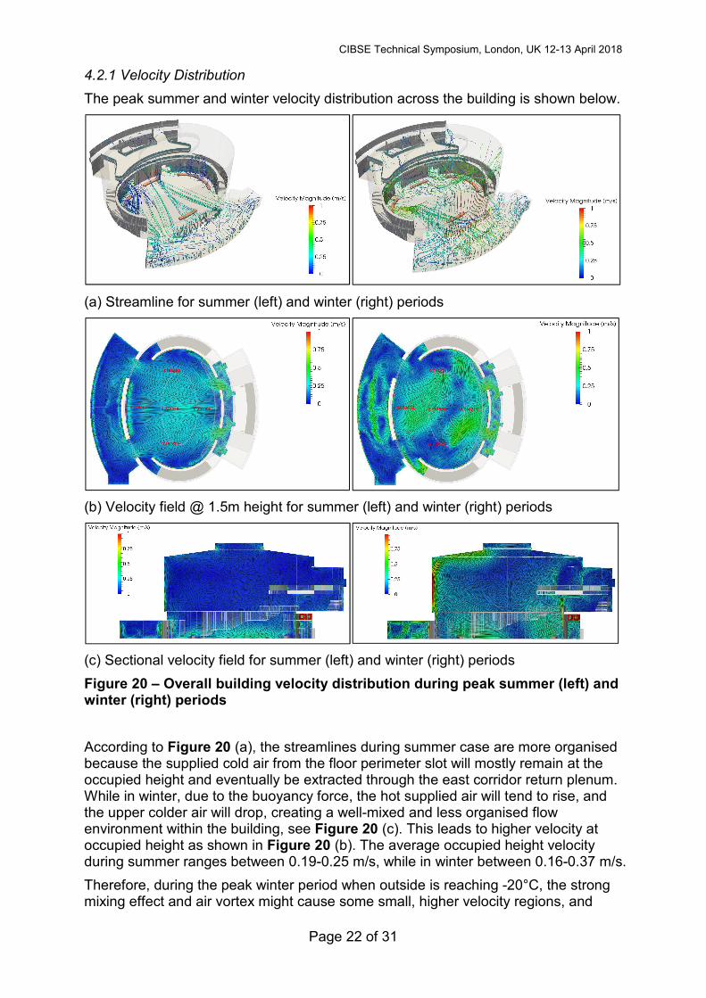
The peak summer and winter velocity distribution across the building is shown below.

(a) Streamline for summer (left) and winter (right) periods

(b) Velocity field @ 1.5m height for summer (left) and winter (right) periods

(c) Sectional velocity field for summer (left) and winter (right) periods

Figure 20 – Overall building velocity distribution during peak summer (left) and winter (right) periods

According to Figure 20 (a), the streamlines during summer case are more organised because the supplied cold air from the floor perimeter slot will mostly remain at the occupied height and eventually be extracted through the east corridor return plenum. While in winter, due to the buoyancy force, the hot supplied air will tend to rise, and the upper colder air will drop, creating a well-mixed and less organised flow environment within the building, see Figure 20 (c). This leads to higher velocity at occupied height as shown in Figure 20 (b). The average occupied height velocity during summer ranges between 0.19-0.25 m/s, while in winter between 0.16-0.37 m/s.

Therefore, during the peak winter period when outside is reaching -20°C, the strong mixing effect and air vortex might cause some small, higher velocity regions, and


of 31

lead to potential local discomfort. The current study assumed an over-pressurisation rate of 17%. During the real operation, different extract fan control strategies can be used, to balance the over-pressurisation and maintain a more uniform velocity region.

4.2.2 Temperature Distribution

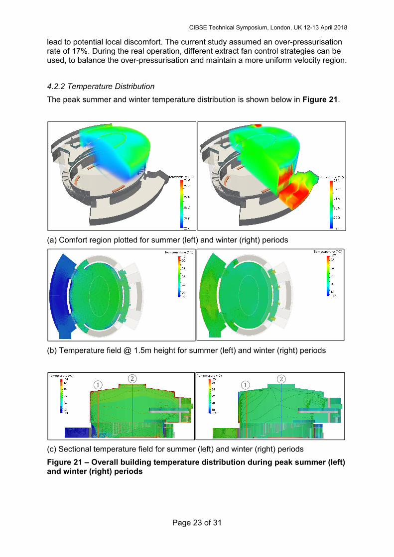
The peak summer and winter temperature distribution is shown below in Figure 21.

(a) Comfort region plotted for summer (left) and winter (right) periods

(b) Temperature field @ 1.5m height for summer (left) and winter (right) periods

(c) Sectional temperature field for summer (left) and winter (right) periods

Figure 21 – Overall building temperature distribution during peak summer (left) and winter (right) periods

② ①

② ①


of 31

Figure 21 (a) plots the areas within comfort region in colour, with the colour scale of ±1°C from the setpoints. From the results, this novel UFAD system can provide sufficient cooling/heating for both summer and winter cases.

In summer, the legacy gallery looks slightly over-cooled based on the scale used in Figure 21 (b). This is because only one AHU is serving all of 6 splash boxes without zonal re-heat control, therefore, the legacy gallery is slightly cooler, at around 23°C. However, this is still within the setpoint control range (23.9 ±1°C) determined for the legacy gallery, which is around 3°C cooler than the main hall. In addition, there are two FCUs within the legacy gallery. If required, they will be activated by the BMS system and provide zonal temperature adjustment.

The vertical temperature stratification profiles across two typical section lines in Figure 21 (c) are plotted in Figure 22.

Figure 22 – Temperature plot along the building height, cut through section ① (left) and ② (right), during summer (top) and winter (bottom)

According to ASHRAE 55-2013 (12), a maximum of temperature variation between ankle-to-head height should be within 3°C to ensure local comfort. According to the temperature plot, both the summer and winter cases can meet this criterion. The plot also shows the temperature variation within the plenum (in profile line 1), to demonstrate the heat release/pick up rate.

During winter, the temperature drop at ceiling level caused by cold skylight surface is more obvious in the central area according to Figure 22. Along the glass-line, the

trench heating supply maintained uniform temperature to prevent cold downdraught.

In summer, more thermal stratification is observed near the glass, due to the high glazing temperature. Overall, the stratification effect is not strong during summer, mainly because of the trench boost system along the glass-line, and the mezzanine café displacement ventilation systems. However, as can be seen in Table 6, the system is far from reaching its maximum cooling capacity and only supplies at 24.8°C


of 31

to meet necessary cooling demand. A test run was carried out, to assess the performance of the building without the trench boost during peak summer period. As shown in Figure 23, when turning OFF the trench supply, there is a much stronger stratification observed, which also caused slight overheating in the entrance and café areas.

Therefore, a strong stratification similar to the normal UFAD system is expected, if this type of system is used in a normal office-type building, under the peak summer condition.

Figure 23 – Temperature field plot with (left) and without (right) glass trench supply during peak summer condition

For both summer and winter cases, the floor is not significantly cooling/heating the space. This is because that the peak time is determined based on the AHU peak coil load. There is a temperature delay in the floor build-up, known as ‘thermal decay’ (10). This will be discussed in the next chapter, along with the radiant effect brought by the system.

4.3 Annual Thermal Comfort and Part Load Performance

4.3.1 Thermal Decay Effect and Annual Radiant Thermal Comfort

Due to the thermal mass of the floor build-up, there will be a thermal decay effect between the floor plenum temperature and room floor surface temperature. Figure 24 uses the winter peak day temperature distribution to demonstrate this effect, as the solar load can easily affect the floor surface temperature in summer. The graph is plotted taken the floor surface above one of the central splash box (flow-zone 3_5), to better capture the supply air temperature variation from the AHU. It can be observed that around 3 hours’ time-lag exists in the morning for the floor to reach peak temperature, using the current case-study build-up. Afterwards it can provide radiant heating effect and further improve occupants’ thermal comfort.


of 31

Figure 24 – Thermal decay effect under peak winter day

OpenFOAM CFD could integrate the radiation and moisture transfer model to capture the mean radiant temperature and relative humidity distribution within the space. However, solving these variables within a 26 million cell size model is computational-expensive. On the other hand, IES-VE can generate zonal averaged results for relative humidity and mean radiant temperature, which are sufficient to demonstrate thermal comfort level within the space. Using CBE thermal comfort tool (20), under the setpoint of 21.1°C-26.7°C, mean air velocity of 0.2 m/s (averaged value based on Figure 20), relative humidity of 50%, metabolic rate of 1.2 met (standing, relaxed), and the clothing level of 0.5 (summer) – 1.0 (winter), the threshold of mean radiant temperature (MRT) target specified for the space is between 18.4-28.0°C, to meet ASHRAE 55 standard (-0.5<PMV<0.5) (12). An annual MRT graph for the central hall is plotted using IES-VE as below in Figure 25:

Figure 25 – Annual MRT plot for the hall central occupied area

It is shown above that the current system and control strategy can provide 84% hours comfort within the occupied hours (11:00-20:00), with 11% overheating hours and 5% underheating hours. This was partially because the basis of design temperature set is slightly high for summer (26.7°C). The system has extra capacity, as discussed

00:00

24:00


of 31

before, to further reduce the room temperature during the real operation and improve the thermal comfort.

If minor system control adjustments can be made during the operational stage, the building has potential meet the requirements of at least 5 directly-related features under WELL building standard – 03 Ventilation Effectiveness, 16 – Humidity Control, 21 Displacement Ventilation, 76 – Thermal Comfort, and 83 – Radiant Thermal Comfort (21).

4.3.2 Comparison between the Novel UFAD System and Traditional Displacement Ventilation (DV) System

A comparative study was done to demonstrate the improved radiant thermal comfort brought by the novel UFAD system in the case study building. An IES-VE annual model was run for the main hall area, using traditional DV system. The supply air speed through perimeter slots, temperature/humidity setpoints, CAV control strategies, economizers, etc. are all identical for both systems, only the floor plenum was removed for the DV system model. From the results, although both systems can achieve the same air temperature and humidity setpoints, there’s some difference between the floor surface temperature. Figure 26 plotted the hall floor surface temperatures comparison between two systems, under both peak summer and winter conditions.

Figure 26 – Floor temperature difference using two systems

It can be observed that the novel UFAD system can improve both summer and winter floor temperatures, and create more radiant comfort environment. Annually, as shown in Figure 27, using the novel UFAD system can achieve 14% more comfort hours. Winter temperature enhancement is more significant than the summer, due to larger temperature difference between indoor and outdoor.

0.0

5.0

10.0

15.0

20.0

25.0

30.0

35.0

40.0

1 1 : 3 0 1 2 : 3 0 1 3 : 3 0 1 4 : 3 0 1 5 : 3 0 1 6 : 3 0 1 7 : 3 0 1 8 : 3 0 1 9 : 3 0 2 0 : 3 0

TE

MP

ER

AT

UR

E (

°C)

Winter Novel UFAD System Winter DV System Summer Novel UFAD System Summer DV System


of 31

Figure 27 – Annual comfort hours comparison between two systems

Energy-wise, it can be seen from Figure 28 that, under the same fan operation and control strategies, the novel UFAD system can save around 6% energy consumption comparing to the traditional DV system.

Figure 28 – Energy consumption comparison between two systems


of 31

4.3.3 Humidity Control and Re-heating Coil Demand

Humidity control is important especially for functions like museum and gallery. To meet 50% RH% design target for the space, there is a re-heating coil in the AHU to provide elevated supply temperature after dehumidification. By using the validated IES-VE system model, it is possible to visualise the annual heating coil demand and size the coil size properly, or allow sufficient hot water supply during summer periods.

Figure 29 – Annual heating coil demand in the system AHU

It can be observed in Figure 29 that even though the peak heating demand is around 350 kW during the winter, there is around 150 kW re-heating load demand during summer for dehumidification purposes. Therefore, the hot water capacity should also be allowed during that period. To reduce the re-heating load, various strategies can be used such as return air by-pass dampers, solar hot water, condenser water heat recovery and so on.

5.0 Conclusion and Further Recommendations

A multi-software coupled modelling method was used in this research using DSM software IES-VE and CFD software OpenFOAM. A validated analytical model was developed for a novel UFAD system, within a case study building (SC Johnson’s Fortaleza Hall). Using the method outlined in this research, the airflow model can reach nearly 100% alignment within the flow-zones, between IES-VE and OpenFOAM CFD. The temperature alignments between two models are 93.3% in summer (6.7% percentage error) and 97.5% in winter (2.5% percentage error). This coupled model can be used in many engineering studies such as assessing building overall peak load performance, and annual simulation for the part load optimisation.


of 31

It is shown from CFD peak period analysis that, both summer and winter indoor temperature can be maintained within ±1°C of setpoints. In summer, the stratification effect is not as obvious as expected, mainly because of the additional trench supply system along the glass-line and the displacement ventilation system at the mezzanine café level. It is also observed that when using the novel UFAD System in the large public space, the local splash box terminal control should be provided to obtain better zonal temperature and humidity control.

From the annual analysis using IES-VE, it is shown that the novel UFAD system in the case study building can lead to at least 84% of annual comfort hours under ASHRAE 55-2013 standard, which is 14% more comparing to traditional displacement ventilation system, and can save around 6% energy consumption at the same time. With minor adjustment on the setpoint control, the project can potentially meet 5 directly-related feature requirements for the WELL standard, to show the enhanced thermal performance. An annual heating coil load was also plotted to illustrate the estimated summer re-heating load and their impact on the humidity control and heating coil sizing.

To ensure the sufficient air speed and movement in the central hall area, the CAV operation was assumed for this study. Potentially, the system can also operate using VAV control. However, the flow model validated in this study was based on the maximum supply velocity. At the reduced airflow, the zonal airflow transfer might need to be adjusted. Therefore, for the future study, a variable flow model can be developed and then the part load performance under VAV operation can be more accurately assessed.

References (1) Airfloor, Airfloor Overview, Accessed on 19th November 2017, Available from:

https://www.airfloor.com/. (2) Price Industries Ltd., Engineer’s HVAC Handbook: Edition 1 – A Comprehensive

Guide to HVAC Fundamentals, Winnipeg: Price Industries Ltd., 2012, pp. 835-859. (3) Candaroma J.P., Flores A.J., Lagman D.H., Tenorio N.C. & Vasquez V.J.,

Performance Comparative Analysis of Ducted and Plenum Underfloor Air Distribution (UFAD) System using ANSYS CFD, Bachelor of Science thesis, Mapua University, 2014.

(4) American Society of Heating, Refrigerating and Air-Conditioning Engineers (ASHRAE), ANSI/ASHRAE Standard 62.1-2013, Ventilation for Acceptable Indoor Air Quality, Atlanta: ASHRAE, 2013.

(5) Schiavon S., Lee K.H., Bauman F. & Webster T., Simplified calculation method for design cooling loads in underfloor air distribution (UFAD) systems, Accessed on 26th November 2017, Available from: https://escholarship.org/uc/item/5w53c7kr.

(6) Centre for the Built Environment (CBE), UC Berkeley, UFAD Cooling Load Design Tool, Accessed on 26th November 2017, Available from: https://www.cbe.berkeley.edu/ufad-designtool/online.htm.

(7) ASHRAE, UFAD Guide: Design, Construction and Operation of Underfloor Air Distribution Systems, Atlanta: ASHRAE, 2013.

(8) Linden P.F., Yu J.K., Webster T., Bauman F., Lee K.H., Schiavon S. & Daly A., Simulation of Energy Performance of Underfloor Air Distribution (UFAD) Systems,


of 31

Accessed on 26th November 2017, Available from: https://escholarship.org/uc/item/1tq6n6pz.

(9) Park B., Thermal Analysis of Hollow Core Ventilated Slab Systems, PhD thesis, University of Colorado at Boulder, 2016.

(10) Webster T., Bauman F., Buhl F. & Daly A., Modeling of Underfloor Air Distribution (UFAD) Systems, Third National Conference of IBPSA-USA, Berkeley, California, IBPSA, 2008.

(11) Chapman K.S., White Paper: Relative Humidity Impacts of the AirFloor System in the Built Environment, Accessed on 19th November 2017, Available from: https://www.airfloor.info/wp-content/uploads/2017/09/Humidity-Impact-of-AirFloor-Systems3036.pdf.

(12) ASHRAE, ANSI/ASHRAE Standard 55-2013, Thermal Environmental Conditions for Human Occupancy, Atlanta: ASHRAE, 2013.

(13) Chapman K.S., Airfloor Downward Losses in an Unconditioned, Well-Ventilated Space, Accessed on 26th November 2017, Available from: https://www.airfloor.info/wp-content/uploads/2017/09/Downward-Losses-in-an-Unconditioned-Well-Ventilated-Space_Kirby-Chapmann.pdf.

(14) SC Johnson, SC Johnson’s Fortaleza Hall Awarded LEED Gold Certification, Accessed on 26th November 2017, Available from: http://www.scjohnson.com/en/press-room/press-releases/05-12-2011/SC-Johnson%E2%80%99s-Fortaleza-Hall-Awarded-LEED-Gold-Certification.aspx.

(15) OpenFOAM, OpenFOAM Official Website, Accessed on 26th November 2017, Available from: https://www.openfoam.com/.

(16) Integrated Environmental Solutions, IES-VE Official Website, Accessed on 26th November 2017, Available from: https://www.iesve.com/.

(17) Openfoamwiki, The Simple Algorithm in OpenFOAM, Accessed on 26th November 2017, Available from: http://openfoamwiki.net/index.php/.

(18) Launder, B.E., Spalding, D.B., Turbulence Models and Their Application to the Prediction of Internal Flows, Journal of Meteorology (Volume 68), 1971.

(19) O’Sullivan, N., Landwehr, S., Ward, B., 2013. Mapping Flow Distortion on Oceanographic Platforms using Computational Fluid Dynamics, Ocean Science (Volume 9), 2013, pp. 855–866.

(20) Centre for the Built Environment (CBE), UC Berkeley, CBE Thermal Comfort Tool, Accessed on 28th November 2017, Available from: http://comfort.cbe.berkeley.edu/.

(21) International WELL Building Institute (IWBI), The WELL Building Standard v1 with Q4 2017 Addenda, Accessed on 1st December 2017, Available from: https://www.wellcertified.com/node/3423.

Acknowledgements The authors wish to firstly thank Sergey Mijorski from SoftSim Consult, who developed the prototype workflow with us when he was working for Foster + Partners. We would like to also thank the lead project architect Jorge Uribe (Foster + Partners) and lead MEP engineer Bud Spiewak (Cosentini) for kindly supporting us and sharing the necessary information for this research. Lastly, we would like to thank Anis Abou-Zaki and Vagelis Giouvanos from Foster + Partners’ Environmental Engineering team for kindly providing their comments and feedback for this research.

assessing thermal comfort and performance of the airfloor ......to enhance air quality and radiant...

Documents