assessing the impacts of enso-related weather the impacts of enso-related weather effects on the...

Assessing the Impacts of ENSO-related weather

effects on the Brazilian Agriculture1

Paulo Araújo Universidade Federal de Viçosa (UFV)

José Féres

Instituto de Pesquisa Econômica Aplicada (IPEA)

Eustáquio Reis Instituto de Pesquisa Econômica Aplicada (IPEA)

Marcelo José Braga

Universidade Federal de Viçosa (UFV)

Abstract

This paper aims at assessing the impacts of ENSO events on the Brazilian agricultural production. The analysis is focused in the Northeast and South regions, the most vulnerable to ENSO effects in Brazil. We adopt a three-stage approach. First, we specify a spline regression model relating sea surface temperature anomalies (SSTA) in the Pacific to weather conditions in Brazilian municipalities. Then, we specify a second group of regressions aimed at assessing how temperature and precipitation in Brazilian municipalities determine crop yields. Finally, with the estimated coefficients provided by the regressions of the early stages, we conduct simulation exercises to evaluate the impacts of ENSO on crop yields. Simulation results show that corn and bean production are quite vulnerable to El Niño effects in the Northeast region, with productivity losses reaching 50%. The critical impact on corn and bean has important socioeconomic consequences, since these crops are mainly produced by household farmers. We also found that the impact of La Niña in the South region is quite significant for all crops.

1 The authors would like to acknowledge the financial support provided by Rede-CLIMA/FAPESP and

NEMESIS research network (FAPERJ/PRONEX).

1. Introduction

The El-Niño-Southern Oscillation (ENSO) is the most important coupled ocean-atmosphere phenomenon to cause global climate variability on interannual time scale. Basically, the phenomenon is related to the quasi-periodic redistribution of heat across tropical Pacific. ENSO is characterized by a varying shift between a neutral phase and two extreme phases: El Niño and La Niña2. The El Niño phase is marked by a deep layer of warm ocean water across the east-central equatorial Pacific, with sea surface temperatures generally 1.5°-2.5° above average. La Niña related conditions are opposed to those of El Niño: a deep layer of cooler than average ocean temperatures across the east-central equatorial Pacific, with sea-surface temperatures generally 1.0°-2.0° below average.

The life cycle and strength of a Pacific warm or cold have significant weather impacts which are felt across large geographic areas. For example, the strong 1982-1983 El Niño led to heavy rains in the United States, India and China. On the other hand, during this period Australia and Northern Africa experienced severe droughts.

In Brazil, weather-related effects associated to El Niño and La Niña vary considerably across regions. During the El Niño phase, there is a reduction in precipitation in the North and Northeast regions, while the South region faces a higher frequency of heavy rains. In La Niña years, the situation is reversed: while the North-Northeast regions experience higher than average rainfalls, the South region is subject to severe droughts.

ENSO events have significant effects on rural activities, since weather is a primary determinant of agricultural productivity. Disruption of agricultural activities due to ENSO-related events may impose substantial social and economic costs, leading to food price increases as well as decreasing rural incomes. According to Berlato et al. (2005), agricultural production losses in Brazil amounted to 4.9 million tons during the 1982-1983 El Niño. Floodings caused a 35% decrease in agricultural production in the South region, while the severe droughts affected 29 million people in the Northeast region.

This paper aims at assessing the impacts of ENSO events on the Brazilian agricultural production. The analysis is focused in the Northeast and South regions, the most vulnerable to ENSO effects in Brazil. Using a database for 1970-2002, we specify an econometric model to analyze how ENSO events have impacted crop yields in each region.

The paper is organized as follows. After this introduction, the next section provides further details of ENSO effects on Brazilian weather. The third section describes the econometric model and the database.Results are presented and discussed in the fourth section. Finally, the last section provides a synthesis of the main conclusions.

2 See Appendix A for the evolution of ENSO phases during the period considered in this paper.

2. ENSO-related weather effects in Brazil

ENSO-related weather effects are quite heterogeneous across Brazilian regions. Generally speaking, one may observe a reduction in precipitation in the North and Northeast regions during the El Niño phase, while the South region faces a higher frequency of heavy rains. In La Niña years, the situation is reversed: while the North-Northeast regions experience higher than average rainfalls, the South region is subject to severe droughts3.

As can be seen in Table 1, during El Niño years average monthly rainfall in the Brazilian Northeast decreases considerably when compared to neutral years. Higher average temperatures are also verified during all the seasons. On the other hand, La Niña years are characterized by higher precipitation and slightly lower temperatures. ENSO-related episodes have also an impact on the frequency of extreme precipitation events in the Northeast region, with the occurrence of severe droughts during El Niño and floodings during la Niña years.

Table 1 – Average monthly precipitation (mm) and temperature (oC) in the Northeast region during El Niño, La Niña and neutral periods.

Northeast Neutral El Niño

1982-83

El Niño

1997-98

La Niña

1973-76

La Niña

1986-89

Precipitation (mm)

Summer 91.80 84.13 74.23 95.37 108.08

Autumn 139.23 94.23 110.51 163.16 185.81

Winter 66.05 47.96 56.23 70.53 78.45

Spring 38.4 25.30 25.67 52.96 38.96

Temperature (oC)

Summer 26.27 26.52 27.08 26.13 26.39

Autumn 25.41 25.70 26.07 25.12 25.79

Winter 23.80 24.31 24.45 23.48 23.75

Spring 25.78 26.11 26.66 25.41 26.05

Source: CPTEC.

ENSO-related effects in the South region are opposed to the ones found in Northeast. As showed in Table 2, El Niño years register higher precipitation levels and lower temperatures. The frequency of heavy rains increases considerably and flooding episodes are regularly observed. On the other hand, during the La Niña phase, average monthly rainfall decreases and temperatures are higher. Both the floodings associated to the El Niño phase and the severe droughts associated to La Niña are responsible for significant agricultural production losses in Southern Brazil.

3 CPTEC (2001).

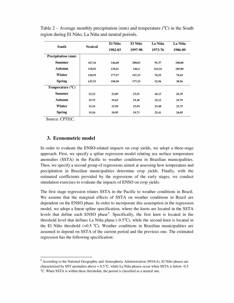
Table 2 – Average monthly precipitation (mm) and temperature (oC) in the South region during El Niño, La Niña and neutral periods.

South Neutral El Niño

1982-83

El Niño

1997-98

La Niña

1973-76

La Niña

1986-89

Precipitation (mm)

Summer 167,16 146,60 200,03 95,37 108,08

Autumn 118,92 139,61 146,4 163,16 185,80

Winter 120,59 177,57 147,33 70,35 78,45

Spring 147,53 190,50 177,33 52,96 38,96

Temperature (oC)

Summer 23,23 23,09 23,51 26,13 26,39

Autumn 19,75 19,65 19,30 25,12 25,79

Winter 15,16 15,50 15,94 23,48 23,75

Spring 19,26 18,95 19,71 25,41 26,05

Source: CPTEC.

3. Econometric model

In order to evaluate the ENSO-related impacts on crop yields, we adopt a three-stage approach. First, we specify a spline regression model relating sea surface temperature anomalies (SSTA) in the Pacific to weather conditions in Brazilian municipalities. Then, we specify a second group of regressions aimed at assessing how temperature and precipitation in Brazilian municipalities determine crop yields. Finally, with the estimated coefficients provided by the regressions of the early stages, we conduct simulation exercises to evaluate the impacts of ENSO on crop yields.

The first stage regression relates SSTA in the Pacific to weather conditions in Brazil. We assume that the marginal effects of SSTA on weather conditions in Brazil are dependent on the ENSO phase. In order to incorporate this assumption in the regression model, we adopt a linear spline specification, where the knots are located in the SSTA levels that define each ENSO phase4. Specifically, the first knot is located in the threshold level that defines La Niña phase (-0.5oC), while the second knot is located in the El Niño threshold (+0.5 oC). Weather conditions in Brazilian municipalities are assumed to depend on SSTA of the current period and the previous one. The estimated regression has the following specification:

4 According to the National Geographic and Atmospheric Administration (NOAA), El Niño phases are

characterized by SST anomalies above + 0.5 oC, while La Niña phases occur when SSTA is below -0.5

oC. When SSTA is within these thresholds, the period is classified as a neutral one.

weatherit = β0 + ӏӏ(SSTA ≤ -0.5 o

C)β1 SSTAt + ӏӏ(-0.5 o

C ≤ SSTA≤ 0.5 o

C)β2 SSTAt + ӏӏ(SSTA ≥ 0.5 o

C) β3

SSTAt + ӏӏ(SSTA ≤ -0.5 o

C) β4 SSTAt -1 + ӏӏ(-0.5 o

C ≤ SSTA ≤ 0.5 o

C) β5 SSTAt -1 + ӏӏ(SSTA ≥ 0.5 o

C) β6

SSTAt-1 + β7 latiti*SSTAt + β8 longiti*SSTAt + µi + εit (1)

where variable weather refers to observed temperature and precipitation levels in municipality i in quarter t , variables SSTAt and SSTAt-1 refer to sea surface temperature anomalies observed in the current quarter and the previous one, and µi is a fixed effects term that accounts for unobserved geographic characteristics of the municipality that may influence weather conditions. In other to account for the heterogeneity of ENSO effects across the country, we also introduce cross-product terms where the geographical location characteristics of the municipality (latitude and longitude) are multiplied by SSTA.

The second stage regression relates crop yields with observed temperature and precipitation. In order to incorporate the non-linearity relations between crop productivity and weather, we introduce both linear and quadratic terms for the wheater variables. The estimated regression has the form:

itiititititsit Tprecprectemptempyield ηµγγγγγγ +++++++= 52

432

210 (2)

where variable yield refers to crop productivity of crop s in municipality i in year t measured in terms of yield/hectare. Temp and prec represent observed temperature and precipitation. The weather related variables were introduced in quarterly averages, in order to account for the potential heterogeneity weather variations may have on crops in different seasons of the year. Variable T represents a time trend included in the regression in order to account technological progress and other time-varying unobserved characteristics common to all municipalilities that may affect crop productivity.

Finally, the third stage refers to the simulation exercise. In order to assess the effects of El Niño/La Niña on crop productivity, we adopt the following simulation approach:

E(∆yield )El Niño=

− ][][´

^^^

neutralElNiño weatherEweatherEγ (3)

E(∆yield )La Niña=

− ][][´

^^^

neutralLaNiña weatherEweatherEγ (4)

where

=

^

4

^

3

^

2

^

1 ,,, γγγγγ is the estimated weather-related coefficients of the second

stage regression (equation (2)) and ][^

weatherE is the estimated temperature and

precipitation regarding each ENSO phase obtained in the first-stage regression.

Data

The econometric model was estimated using data for the period 1970-2002. Agricultural information was obtained from the Produção Agrícola Municipal (PAM), a yearly agricultural survey conducted by the Instituto Brasileiro de Geografia e Estatística (IBGE - Brazilian Institute of Agriculture and Statistics). PAM provides data on total production and planted area by crop for each Brazilian municipality. Crop yields were computed by dividing total production by planted area. For our analysis, we chose the most important crops in terms of production value in each region. Appendix B provides crop productivity maps for both Northeast and South regions.

Observed temperature and precipitation data was obtained from the database CL 2.0 10’, produced by the Climate Research Unit (CRU/University of East Anglia). This database provides monthly data at a 50 km horizontal resolution grid. Municipal weather averages were obtained by overlaying the climate grid on the Brazilian municipality map, using ArcGIS software. Finally, data on SSTA was obtained from NOAA.

4. Results

The model was estimated for a panel of 1,855 municipalities covering the period 1970-2002. Regression results for equations (1) and (2) are presented in Appendix C.

Estimated coefficitents from the first-stage regression indicate that variations in sea surface temperature in the Pacific Ocean have distinct effects on weather in Brazilian municipalities according to ENSO phase. In particular, controlling for geographical characteristics, increasing temperatures in the Pacific during El Niño periods leads to higher temperatures and lower precipitation in Brazilian municipalities.

Results from the second stage regressions shows that weather coefficients vary considerably by season, suggesting that impact of temperature and precipitation variations are quite heterogenous across seasons. This finding highlights the importance of working with disaggregated weather-related data, since annual data would not be able to capture such pattern. It should also be remarked that in most of the regressions both linear and quadratic terms for weather variables are significant, showing the non-linearity relationship between weather and crop productivity.

Tables 3 and 4 exhibit the simulation results for the impact of ENSO events on Northeast and South regions, respectively. During El Niño years, sugarcane and manioc productivity in Northeast decrease by 5%. Corn and bean production are quite more vulnerable, with productity losses reaching 50%. The critical impact on corn and bean has important socioeconomic consequences, since these crops are mainly produced by household farmers. Regarding La Niña, the effects on sugarcane and manioc may be considered negligible, but the impact is quite severe on bean productivity.

Table 3: Impact of ENSO events on crop productivity – Northeast Region

Crop

Average

Productivity

(tons/ha)

El Niño La Niña

∆ productivity

(tons/ha)

Percentage

change ∆ productivity

(tons/ha)

Percentage

change

Sugarcane 21.29 -0.91 -4.3% -0.07 -0.3%

Manioc 1.88 -0.10 -5,3% -0.01 -0.5%

Corn 0.52 -0.28 -53,8% -0.03 -5.7%

Bean 0.37 -0.18 -48.6% -0.15 -40.5%

Table 4 shows that the impact of La Niña in the South region is quite significant for all the crops. Actually, during la Niña phase, the South region is subject to severe droughts which may lead to significant production loss. Wheat production seems particularly vulnerable to La Niña effects. The effects of El Niño are also significant, particularly for corn and soybean production.

Table 4: Impact of ENSO events on crop productivity – South Region

Crop

Average

Productivity

(tons/ha)

El Niño La Niña

∆ productivity

(tons/ha)

Percentage

change ∆ productivity

(tons/ha)

Percentage

change

Corn 2.37 -0.96 -40.5% -1.23 -51.9%

Rice 2.14 -0.01 -0.4% -0.25 -11.7%

Wheat 0.78 -0.05 -6.4% -0.67 -85.9%

Soybean 1.22 -0.96 -78.7% -0.32 -26.2%

Figure 1: ENSO effects on crop productivity – Northeast Region

Figure 2: ENSO effects on crop productivity – South Region

5. Conclusion

ENSO events have significant effects on rural activities, since weather is a primary determinant of agricultural productivity. Disruption of agricultural activities due to ENSO-related events may impose substantial social and economic costs, leading to food price increases as well as decreasing rural incomes. Identifying the impacts of ENSO-related events is of paramount importance to assess crop vulnerability and the correlated socioeconomic consequences.

This paper aimed at assessing the impacts of ENSO events on the Brazilian agricultural production. The analysis was focused in the Northeast and South regions, the most vulnerable to ENSO effects in Brazil. We adopted a three-stage approach. First, we specified a spline regression model relating sea surface temperature anomalies (SSTA) in the Pacific to weather conditions in Brazilian municipalities. Then, we specified a second group of regressions aimed at assessing how temperature and precipitation in Brazilian municipalities determine crop yields. Finally, with the estimated coefficients provided by the regressions of the early stages, we conducted simulation exercises to evaluate the impacts of ENSO on crop yields.

Simulation results showed that corn and bean production are quite more vulnerable to El Niño effects in the Northeast region, with productity losses reaching 50%. The critical impact on corn and bean has important socioeconomic consequences, since these crops are mainly produced by household farmers. We also found that the impact of La Niña in the South region is quite significant for all the crops.

Biblioghaphy

BERLATO, M. A. et al. (2005). “Associação entre El Niño Oscilação Sul e a produtividade do milho no Estado do Rio Grande do Sul”. Pesquisa Agropecuária

Brasileira. Brasília: n. 5, v. 40, p. 423-432.

CPTEC-INPE. Centro de Previsão de Tempo e Estudos Climáticos, Instituto Nacional de Pesquisas Espaciais. Acessed in: nov. 2011. Available at: http://www.cptec.inpe.br/

DENG, X. et al. Impacts of El Nino-Southern Oscillation events on China’s rice production. Journal of Geographical Sciences. V.20, p. 3-16, 2010.

DÊSCHENES, O.; GREENSTONE, M. (2007) The economic impacts of climate change: evidence from agricultural output and random fluctuations in weather. American Economic Review. Ed. 97, v.1, p. 354-385. GOULD, W. Linear Splines and piecewise linear functions. Stata Technical

Bulletin. Set. 1993.

IBGE. Instituto Brasileiro de Geografia e Estatística. Acesso em: nov. 2011. Disponível em: www.ibge.gov.br

LEGLER, D. M.; BRYANT, K. J.; O’BRIEN, J. J. Impact of ENSO-related climate anomalies on crop yields in the US. Climatic Change. 1998.

Appendix A: Evolution of ENSO regimes during 1970-2002

Ano Fenômenoa

Ano Fenômenoa

1970 La Niña 1992 El Niño


1972 El Niño 1994 El Niño

1973 El Niño 1995 La Niña

1974 La Niña 1996 La Niña




1978 Neutro 2000 Neutro

1979 EL Niño 2001 La Niña

1980 El Niño 2002 Neutro

1981 Neutro 2003 El Niño




1985 La Niña 2007 La Niña




1989 La Niña 2011 Neutro

1990 Neutro 2012 La Niña

1991 El Niño

Source: CPTEC – INPE, 2012.

Note: (a) bolded letters identify years where El Niño/La Niña were classified as severe.

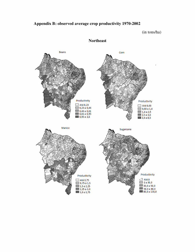
Appendix B: observed average crop productivity 1970-2002

(in tons/ha)

Northeast

South

(in tons/ha)

Appendix C: regression results

First stage: SSTA effects on Brazilian weather

Precipitation (mm) Temperature (oC)

summer autumn winter spring summer autumn winter spring

SSTALaNiña. t

4.12***

(0.1813)

9.836***

(0.3278)

-6.70***

(0.3643)

-1.385***

(0.3633)

-0.0154***

(0.0023)

-0.065***

(0.0032)

0.1948***

(0.0069)

0.479***

(0.0083)

SSTAneutral. t -3.74***

(0.1882)

1.040***

(0.2418)

-1.48***

(0.1968)

-4.98***

(0.1392)

-0.0118***

(0.0024)

-0.007***

(0.0023)

0.1421***

(0.0038)

0.171***

(0.0031)

SSTAEl Niño. t -0.557***

(0.1412)

1.81***

(0.2319)

-5.54***

(0.2132)

-0.362*

(0.2028)

0.0587***

(0.0018)

0.1022***

(0.0022)

0.214***

(0.0041)

0.214***

(0.0046)

SSTALaNiña. t-1

-5.49***

(0.1583)

-40.47***

(0.9012)

-6.49***

(0.2202)

-0.1370

(0.2388)

0.0347***

(0.0020)

0.2710***

(0.0088)

0.0736***

(0.0042)

-0.323***

(0.0054)

SSTAneutral. t-1 4.63***

(0.1689)

-12.34***

(0.3046)

3.083***

(0.1643)

4.084***

(0.1353)

0.0014***

(0.0022)

0.096***

(0.0029)

-0.095***

(0.0031)

-0.120***

(0.0030)

SSTAElNiño. t-1 -3.36***

(0.1279)

-19.61***

0.5249

-2.936***

(0.1725)

-3.847***

(0.1294)

0.0488***

(0.0016)

0.0302***

(0.0051)

0.140***

(0.0032)

-0.032***

(0.00293)

Latitude -0.050***

(0.0006)

-0.0538***

(0.0001)

-0.048***

(0.00008)

-0.045***

(0.00004)

-0.0518***

(0.00007)

-0.046***

(0.00005)

-0.0458***

(0.00006)

-0.0474***

(0.00005)

Constant 15.77***

(0.3234)

13.47***

(0.5141)

3.01***

(0.3139)

11.553***

(0.1459)

4.122***

(0.0276)

6.27***

(0.0209)

6.35***

(0.0198)

6.088***

(0.0180)

Note: *.** and *** indicate statistical significance at 10%. 5% and 1% level. respectively. Standard errors in parenthesis

Second stage: weather-related impacts on crop yields – Northeast region

Northeast El Niño La Niña

Corn Sugarcane Beans Manioc Corn Sugarcane Beans Manioc

Prec_summer 0.0028***

(0.0002)

0.0243***

(0.0132)

-0.00021*

(0.00014)

0.0015

(0.0013)

-0.0013***

(0.0007)

0.0175**

(0.0228)

-0.0025

(0.00028)

0.0025

(0.00247)

Prec_summer ^2 0.0000006***

(0.00000005)

-0.00007***

(0.0000057)

0.0000

(0.00000)

0.000006

(0.000003)

0.0000006***

(0.0000005)

-0.0001***

(0.000068)

0.0000

(0.0000)

-0.0000009

(0.000007)

Prec_autumn 0.0013***

(0.00019)

-0.0108**

(0.0108)

-0.00013*

(0.00012)

-0.00027

(0.00086)

0.0034***

(0.0002)

0.0186***

(0.0120)

0.0002**

(0.0001)

-0.00002

(0.0014)

Prec_autumn ^2 -0.00000002***

(0.00000007)

0.0000147***

(0.0000054)

0.00000

(0.0000)

-0.000003

(0.00002)

-0.0000007***

(0.0000005)

-0.00005***

(0.000029)

0.0000

(0.0000)

-0.0000006

(0.000003)

Prec_winter 0.0012***

(0.00016)

0.0143**

(0.0127)

-0.00018

(0.00015)

0.0025*

(0.0014)

-0.0010***

(0.0003)

0.0320***

(0.0205)

-0.00005

(0.00015)

0.0013**

(0.017)

Prec_winter^2 -0.00000003***

(0.00000004)

-0.000041***

(0.000039)

-0.0000

(0.00000)

-0.000005**

(0.00006)

0.0000002***

(0.00000007)

-0.000072***

(0.0051)

0.0000

(0.00000)

-0.000003***

(0.000051)

Prec_spring 0.0011***

(0.0004)

0.0121**

(0.0272)

-0.0001

(0.000218)

-0.00311

(0.0022)

0.0013***

(0.0005)

-0.04125*

(0.0303)

0.00003

(0.00003)

-0.0002

(0.0029)

Prec_spring^2 -0.0000006***

(0.0000003)

-0.000008***

(0.000156)

0.0000

(0.00000)

0.0000

(0.00000)

0.0000009***

(0.0000005)

0.0002***

(0.00017)

0.0000

(0.0000)

0.000002**

(0.00005)

Temp_summer 0.7244

(0.1958)

11.96

(9.2034)

0.1161*

(0.0907)

0.1227

(0.6830)

0.1156

(0.1451)

-16.39

(10.327)

0.0665

(0.1230)

0.1532

(0.9059)

Temp_summer

^2

-0.0148**

(0.0037)

-0.21006

(0.17772)

-0.0023

(0.0017)

-0.0027

(0.0128)

-0.0037***

(0.0027)

0.3153*

(0.1945)

-0.0014

(0.0023)

-0.0019

(0.0172)

Temp_autumn -1.0245

(0.1822)

-23.3244**

(12.366)

-0.0733

(0.1214)

-0.6379

(1.0711)

-1.3444

(0.3199)

5.4601

(14.603)

0.0642

(0.1542)

-0.3499

(1.269)

Temp_autumn

^2

0.0217**

(0.0035)

0.4406**

(0.2422)

0.0016

(0.0023)

0.0133

(0.0210)

0.0259**

(0.0060)

-0.1147

(0.2804)

-0.3016

(0.1011)

0.0063

(0.0247)

Temp_winter 0.7407

(0.1284)

-6.2212

(7.05388)

0.0397

(0.0710)

0.6236

(0.5966)

1.5187

(0.2005)

-1.8122

(8.0370)

0.00083

(0.0019)

-0.8812

(0.9486)

Temp_winter^2 -0.01982**

(0.0026)

0.1231

(0.1460)

-0.0006

(0.0014)

-0.0110

(0.0125)

-0.0321**

(0.0037)

0.0421

(0.1606)

0.0025

(0.0811)

0.00171**

(0.019)

Temp_summer -0.9834

(0.1436)

2.406

(8.306)

-0.1743*

(0.0953)

-0.6817

(0.7332)

-0.809

(0.2000)

16.5272

(10.025)

-0.00004

(0.0015)

0.1432***

(0.849)

Temp_summer^2 0.02137**

(0.0027)

-0.04006

(0.1587)

0.0029*

(0.00177)

0.0102

(0.0140)

0.01769***

(0.0040)

-0.3373

(0.1975)

-0.00004

(0.0015)

-0.027*

(0.0169)

Constant 8.318

(2.4915)

20.1613

(10.849)

1.7164

(1.1614)

8.9255

(10.73)

8.4431*

(4.3348)

-16.04

(161.24)

-0.9671

(2.0304)

-3.76

(18.81)

Dummy_1970 1.086***

(0.049)

-1.2201***

(1.193)

0.510***

(0.0019)

0.058*

(0.509) 0.054*

(0.0286)

-0.012***

(0.0286)

0.012**

(0.0003)

0.0174***

(0.0549)

Dummy_1980 0.673***

(0.039)

-10.202***

(1.975)

0.621***

(0.089)

0.0459

(0.189) 0.259***

(0.3195)

-0.037***

(0.0032)

0.034***

(0.0129)

0.0014**

(0.0109)

Dummy_1990 0.210***

(0.052)

-0.460***

(1.541)

0.771***

(0.120)

0.026***

(0.238) 0.4691***

(0.372)

-0.1945***

(0.00344)

0.0815**

(0.0512)

0.0141***

(0.341)

Dummy_2000 0.359***

(0.047)

-0.0945***

(0.02886)

0.9311***

(0.0987)

0.0629**

(0.0255) 1.342***

(0.062)

-0.2021***

(0.0161)

0.1301***

(0.0023)

0.051***

(0.321)


Second stage: weather-related impacts on crop yields – South region

South El Niño La Niña

Rice Corn Soybean Wheat Rice Corn Soybean Wheat

Prec_summer 0.0012

(0.0014) -0.00067

(0.001205) -0.0013

(0.0032)

0.0024**

(0.0013)

-0.0013

(0.0032)

-0.0036

(0.0024)

0.00265**

(0.0015)

-0.00275**

(0.0012)

Prec_summer ^2 -0.000003

(0.000003)

0.0000**

(0.0000)

-0.000002

(0.000009)

-0.000007**

(0.000003)

0.0000

(0.0000)

0.00002***

(0.00000)

-0.000006

(0.000004)

0.000007**

(0.0000003)

Prec_autumn -0.0014

(0.00223) 0.015945***

(0.01612)

0.00012

(0.00166)

-0.000850

(0.0011)

0.00012

(0.0016)

0.00039

(0.00152)

-0.0044***

(0.0011)

-0.00069

(0.00092)

Prec_autumn ^2 -0.00145

(0.0022)

-0.00005***

(0.0000)

0.0000

(0.0000)

0.0000

(0.00000)

0.0000

(0.0000)

0.0000

(0.0000)

0.00001***

(0.000003)

0.000001

(0.0000002)

Prec_winter 0.0000

(0.00000) 0.0005

(0.00098)

-0.0012

(0.0023)

0.00034

(0.00078)

-0.0011

(0.0024)

-0.0021

(0.00169)

0.00091

(0.0014)

0.00085

(0.0014)

Prec_winter^2 0.0001

(0.0015)

0.0000

(0.00000)

0.0000

(0.0000)

0.00000003***

(0.0000)

0.0000

(0.0000)

-0.00001***

(0.0000)

-0.000004

(0.000004)

-0.0000001

(0.000005)

Prec_spring 0.00219

(0.00211) -0.0169***

(0.00203) 0.0000

(0.0000)

-0.00008

(0.0013)

0.0000

(0.0029)

-0.0158***

(0.0023)

-0.015***

(0.0016)

-0.0007

(0.0012)

Prec_spring^2 0.0000

(0.00000)

0.0000***

(0.0000)

0.0000

(0.0000)

0.0000001

(0.000004)

0.0000

(0.0000)

0.0000***

(0.0000)

0.00004***

(0.0000004)

0.000002

(0.0000003)

Temp_summer -0.7000

(0.5519) -0.82296*

(0.4622) -1.0331

(1.034)

-0.1454

(0.2861)

-1.0331

(1.034)

-1.219**

(0.7085)

1.954***

(0.6327)

-0.096

(0.5455)

Temp_summer ^2 0.0144

(0.0111)

0.0062

(0.0100)

0.0199

(0.0216)

0.0031

(0.0061)

0.0197

(0.0216)

0.022

(0.0147)

-0.039***

(0.013)

0.0019

(0.0113)

Temp_autumn -0.2424

(0.2110) 1.866721***

(0.1387) 0.447

(0.6765)

-0.04667

(0.1287)

0.4472

(0.6765)

0.6794

(0.5443)

-0.011

(0.4795)

0.2927

(0.3189)

Temp_autumn ^2 0.0062

(0.0052) -0.04154***

(0.00354) -0.0095

(0.01665)

0.0012

(0.0032)

-0.0095

(0.01665)

-0.0249**

(0.01333)

-0.0031

(0.012)

-0.0073

(0.000783)

Temp_winter 0.1021

(0.1821) -0.61802***

(0.1555) -0.59886**

(0.3066)

-0.0122

(0.1042)

-0.598**

(0.3066)

-1.301***

(0.1991

-0.5164***

(0.1761)

-0.2034

(0.1407)

Temp_winter^2 -0.0029

(0.0053) 0.025976***

(0.0048) 0.01866**

(0.01015)

0.00015

(0.0031)

0.0186**

(0.0105)

0.05852***

(0.0064)

0.02159***

(0.0059)

0.0063

(0.0045)

Temp_summer 0.3522]

(0.3313) 1.280153***

(0.1813) 0.6867*

(0.419)

0.1507

(0.1425)

0.6867*

(0.4190)

4.004***

(0.3316)

-0.3311

(0.2498)

0.1382

(0.2670)

Temp_summer^2 -0.0088

(0.00881) -0.02769***

(0.0044) -0.0167

(0.0106)

-0.0039

(0.0035)

-0.016**

(0.0106)

-0.09844***

(0.0082)

0.010*

(0.0063)

-0.0031

(0.0067)

Constant 8.589

(5.951) -13.5997***

(0.0044) 8.231

(9.109)

1.4998

(2.7350)

8.234

(9.109)

-16.948***

(6.3187)

-14.62***

(5.005)

-0.6574

(4.973)

Dummy_1970 0.006***

(0.0009)

0.036

(0.003)

0.4410***

(0.0999)

0.0014**

(0.0006) 0.1185

(0.0884)

0.0060**

(0.0031)

0.0031***

(0.0008)

0.1217

(0.2224)

Dummy_1980 0.009***

(0.001)

-0.0012

(0.006)

0.0159***

(0.0033)

-0.00028

(0.00069) 0.0114 (0.109)

0.315**

(0.1316)

0.0237***

(0.0007)

-0.0202

(0.1313)

Dummy_1990 0.009***

(0.002)

0.031***

(0.002)

1.081***

(0.2080)

-0.00037

(0.0005) 0.127**

(0.043)

-0.0043

(0.003)

0.0027***

(0.0006)

0.00016

(0.0032)

Dummy_2000 0.010***

(0.002)

0.250***

(0.04)

1.026***

(0.0025)

-0.00036

(0.00048) 0.01883 (0.449)

-0.247***

(0.0933)

0.0009

(0.0008)

0.0694

(0.0666)


assessing the impacts of enso-related weather the impacts of enso-related weather effects on the...

Documents