assessing the impacts climate change may
TRANSCRIPT
Assessing the Impacts Climate Change May Have on the State’s Economy, Revenues, and Investment Decisions: Volume 2: Cost of Doing Nothing Analysis Final
State of Maine Department of the Governor's Office of Policy Innovation and the Future (GOPIF) 111 Sewall Street Augusta, Maine 04330
Eastern Research Group, Inc. 110 Hartwell Avenue Lexington, MA 02421
September 29, 2020

i
TABLE OF CONTENTS Table of Contents ........................................................................................................................................... i
List of Figures and Tables ............................................................................................................................. iv
1. Introduction to Cost of Doing Nothing ..................................................................................................... 6
2. Forests, Natural Working Lands, and Carbon Sequestration .................................................................. 11
2.1. Introduction ..................................................................................................................................... 11
2.2. Carbon Sequestration ...................................................................................................................... 11
2.2.1. Results ....................................................................................................................................... 11
2.2.2. Methods .................................................................................................................................... 11
2.3. Natural Lands Jobs and Economics .................................................................................................. 13
2.3.1. Forest Industry .......................................................................................................................... 13
2.3.2. Agricultural Industry ................................................................................................................. 14
2.4. Climate Impacts on Forestry ............................................................................................................ 15
2.5. Climate Impacts on Agriculture ....................................................................................................... 16
3. Blue Carbon ............................................................................................................................................. 17
3.1. Introduction ..................................................................................................................................... 17
3.2. Results .............................................................................................................................................. 17
3.3. Methods ........................................................................................................................................... 19
3.3.1. Data ........................................................................................................................................... 19
3.3.2. Assumptions .............................................................................................................................. 29
3.3.3. Limitations ................................................................................................................................. 30
3.4. Recommendations for Future Analysis ............................................................................................ 31
4. Flood Risk ................................................................................................................................................ 33
4.1. Introduction ..................................................................................................................................... 33
4.2. Results .............................................................................................................................................. 33
4.3. Methods ........................................................................................................................................... 42
4.3.1. Data ........................................................................................................................................... 42
4.3.2. Limitations ................................................................................................................................. 44
4.3.3. Assumptions .............................................................................................................................. 45
4.4. Recommendations for Future Analysis ............................................................................................ 46
5. Erosion of Beaches and Dunes ................................................................................................................ 47
5.1. Introduction ..................................................................................................................................... 47
5.2. Results .............................................................................................................................................. 47
5.3. Methods ........................................................................................................................................... 48

ii
5.3.1. Data ........................................................................................................................................... 48
5.3.2. Assumptions .............................................................................................................................. 54
5.3.3. Limitations ................................................................................................................................. 54
5.4. Recommendations for Future Analysis ............................................................................................ 55
6. Vector-Borne Illness ................................................................................................................................ 56
6.1. Introduction ..................................................................................................................................... 56
6.2. Results .............................................................................................................................................. 56
6.3. Methods ........................................................................................................................................... 57
6.3.1. Data ........................................................................................................................................... 57
6.3.2. Assumptions .............................................................................................................................. 57
6.3.3. Limitations ................................................................................................................................. 57
6.4. Recommendations for Future Analysis ............................................................................................ 57
7. Fishing and Aquaculture Industries ........................................................................................................ 59
7.1. Introduction ..................................................................................................................................... 59
7.2. Results .............................................................................................................................................. 61
7.3. Methods ........................................................................................................................................... 64
7.3.1. Data ........................................................................................................................................... 64
7.3.2. Assumptions and Limitations .................................................................................................... 64
7.4. Recommendations for Future Analysis ............................................................................................ 64
8. High Heat Days and Heat Illness ............................................................................................................. 65
8.1. Introduction ..................................................................................................................................... 65
8.2. Results .............................................................................................................................................. 66
8.3. Methods ........................................................................................................................................... 67
8.3.1. Data ........................................................................................................................................... 67
8.3.2. Assumptions .............................................................................................................................. 67
8.4. Recommendations for Future Analysis ............................................................................................ 67
9. Conclusion ............................................................................................................................................... 69
References .................................................................................................................................................. 70
APPENDIX A. Monetizing Carbon ............................................................................................................ A-78
A.1. Federal Social Cost of Carbon Values .......................................................................................... A-78
A.1.1. 2016 Interagency Working Group Values ............................................................................. A-78
A.1.2. 2018 Interim Social Cost of Carbon Estimates ...................................................................... A-81
A.1.3. Discount Rates ...................................................................................................................... A-82
A.1.4. Social Cost of Carbon Estimates Extrapolated to 2100 ........................................................ A-82
A.2. Market Price of Carbon ................................................................................................................ A-84

iii
A.3. Recommendations for Maine ...................................................................................................... A-84

iv
LIST OF FIGURES AND TABLES Figure 1. Relative Employment of Maine’s Forest Industry by Census Tract ............................................. 13 Figure 2. Relative Employment in the Agricultural Industry by Census Tract ............................................ 15 Figure 3. Maine Social Vulnerability Index and Sea Level Rise (HAT + 8.8 ft) ............................................. 34 Figure 4. Maine Social Vulnerability Index and 1 Percent Annual Change Riverine and Coastal Floodplain (FEMA National Flood Hazard Layer) .......................................................................................................... 35 Figure 6. Total Storm Surge and Sea Level Rise Damages Between 2020 and 2050 .................................. 37 Figure 7. GDP in Maine Between 2020 and 2050 Based on Job Loss Due to Sea Level Rise and Storm Surge ........................................................................................................................................................... 39 Figure 8. Employment in Maine Between 2020 and 2050 Based on Job Loss Due to Sea Level Rise and Storm Surge................................................................................................................................................. 39 Figure 9. The Maine Beaches Region .......................................................................................................... 49 Figure 10. Breakdown of Maine Beaches Visitor Spending in 2018 ........................................................... 50 Figure 11. Impact of Decreased Beach Width on Beach Visitation ............................................................ 51 Figure 12. Visitors at an Eroded Beach ....................................................................................................... 52 Figure 13. Relative Employment by Census Tract, Fishing Industry ........................................................... 60 Figure 14. Preliminary 2019 Commercial Landings by Ex-Vessel Value ...................................................... 61 Figure 15. Populations Vulnerable to High Heat ......................................................................................... 66 Table 1. Sea Level Rise Scenarios Applied Throughout This Report ............................................................. 8 Table 2. Additional Sea Level Rise Scenarios Applied Throughout This Report ............................................ 9 Table 3. REMI Multipliers of Maine’s Economic Output between 2020 and 2050 ..................................... 10 Table 4. Total Carbon Sequestration Lost Due to Land Use Changes ......................................................... 11 Table 5. Model Parameters ......................................................................................................................... 12 Table 6. Impact of Decreased Output on Agriculture-Related Jobs ........................................................... 14 Table 7. Baseline Stock by Resource ........................................................................................................... 17 Table 8. Summary of Area Lost and Social Cost of CO2 Burial Loss (Eelgrass and Salt Marsh) ................... 18 Table 9. Lower Bound Social Cost of CO2 Used in Blue Carbon Analysis .................................................... 19 Table 10. Market Price of CO2 ..................................................................................................................... 19 Table 11. Ecosystem Services Values (2019$/km2/year) ............................................................................ 22 Table 12. Eelgrass—Baseline Area, Area Lost, and Area Remaining by Year ............................................. 23 Table 13. Eelgrass—Carbon Burial Lost by Year.......................................................................................... 23 Table 14. Eelgrass—Social and Market Cost of CO2 Burial Lost (2019$) .................................................... 24 Table 15. Eelgrass—Ecosystems Services Lost (2019$) .............................................................................. 24 Table 16. Salt Marsh—Baseline Area, Area Lost, and Area Remaining by Year ......................................... 25 Table 17. Salt Marsh—Methane (CH4) Emissions Due to Tidal Marsh Crossing Restrictions ..................... 26 Table 18. Salt Marsh—Emissions Factors and Carbon to CO2 Equivalent Conversion ............................... 26 Table 19. Salt Marsh—Net Carbon Burial (Gg CO2 Equivalent/Year) .......................................................... 27 Table 20. Salt Marsh—Social and Market Cost of CO2 Burial Lost (2019$) ................................................ 28 Table 21. Salt Marsh—Ecosystems Services Lost (2019$) .......................................................................... 28 Table 22. Seaweed—Baseline Stocks .......................................................................................................... 29 Table 23. Cumulative Building Losses Due to Sea Level Rise and Riverine Flooding .................................. 36 Table 24. Statewide Annual GDP Loss Due to Job Loss from Flood Exposure ............................................ 37 Table 25. Natural Resource Industry Jobs Exposed to Current and Future Flood Risk ............................... 38 Table 26. Transportation Infrastructure Exposed to Flooding .................................................................... 40 Table 27. Increase in Culverts and Crossings Restricting Tidal Flow with Sea Level Rise ........................... 41 Table 28. Wastewater Treatment Plant Exposure to Sea Level Rise Inundation Flooding ......................... 41

v
Table 29. Annual Storm Probabilities and Storm Surge .............................................................................. 43 Table 30. Capacity (GPD) per Wastewater Treatment Plant ...................................................................... 44 Table 31. Beach and Tourism Economic Loss for Sea Level Rise Scenarios ................................................ 48 Table 32. Dry Beach Loss for Sea Level Rise Scenarios ............................................................................... 50 Table 33. Beach and Tourism Percentage Loss for Sea Level Rise Scenarios ............................................. 51 Table 34. Developed and Undeveloped Dune Loss .................................................................................... 53 Table 35. Lobster Landings by County, 2019 .............................................................................................. 61 Table 36. Sea Surface Temperature Anomalies and Lobster Landings, 2004–2019 ................................... 62 Table 37. Lobster Landings by State, 2004–2016 (Millions of lbs.)............................................................. 63 Table 38. CMIP5 Projections of Average Sea Surface Temperature Anomalies ......................................... 64 Table A-1. Interagency Working Group (2016) Estimates for the Social Cost of Carbon (2007$ per Metric Ton CO2) .................................................................................................................................................. A-79 Table A-2. Interim EPA (2018) Domestic Social Cost of Carbon, 2015–2050 (2016$ per Metric Ton of CO2) ................................................................................................................................................................ A-81 Table A-3. 2016 Interagency Working Group High and Low Social Cost of Carbon Values Extrapolated to 2100 ........................................................................................................................................................ A-82 Table A-4. Forecast of the Market Price of Carbon Based on Regional Greenhouse Gas Initiative Price Projections .............................................................................................................................................. A-84 Table A-5. Summary of Social Cost of Carbon Versus Market Price of Carbon, Extrapolated to 2100 .. A-85

Assessing the Impacts Climate Change May Have on the State’s Economy, Revenues, and Investment Decisions: Cost of Doing Nothing Analysis
6
1. INTRODUCTION TO COST OF DOING NOTHING
The “cost of doing nothing” refers to the estimated losses that the State of Maine and its citizens could incur if the State does not adapt to climate change and make its own contributions to reducing the extent of climate change. The cost of doing nothing is primarily determined based by damage incurred by climate-related hazards, but we have also included losses in sequestration associated with potential climate hazards.
A cost of doing nothing analysis serves several purposes. First, it helps the State set an economic baseline of the costs it will incur if Maine does not undertake adaptation or mitigation action, costs that can be avoided and that can additionally be weighed against the costs of taking action. Second, it defines the benefits of adaptation and mitigation actions, so the State can select those actions that have the greatest chance of reducing damages from climate change.
Understanding the costs of doing nothing provides perspective on the potential benefits of doing something (i.e., mitigation and adaptation
strategies). Thus, Eastern Research Group (ERG) developed these cost of doing nothing estimates, together with a related report on the cost-benefit and cost-effectiveness of various adaptation and mitigation strategies, to help inform strategy recommendations from the Maine Climate Council Working Groups.
We note that Maine should not consider costs as the sole deciding factor in choosing mitigation and adaptation strategies, but rather view them in combination with details that the working groups provide on feasibility and timing, as well as considerations of equity in how different groups will share the risks and burdens related to climate change. It is also important to keep in mind the limitations of each cost we evaluated, as this report focuses on those that are readily quantifiable.
To develop this cost of doing nothing analysis, ERG first completed a statewide vulnerability assessment to identify key characteristics of communities as well as infrastructure and other assets most vulnerable to climate impacts. The team then ran an economic assessment of damages to those communities and assets under a no-action alternative. We intersected the hazard layer (e.g., flooding, heat) with an economic layer (e.g., the value of housing, the value of ecosystems) to help evaluate the exposed value to the hazard. When feasible, we incorporated the extent of damage (e.g., a depth-damage curve that considers how the depth of flooding is tied to damage, in addition to the extent of flooding), which allowed us to move from calculating the exposed value to a damage or loss. Finally, we tried to incorporate the probability of the hazard to move from the damage associated with an event to an expected annual loss over time, which provides more insight into accounting of benefits and costs. To quantify the costs of lost carbon sequestration under the “do nothing” scenario, ERG used the social cost of carbon, which Appendix A discusses in detail. In most chapters of this report, ERG estimates

Assessing the Impacts Climate Change May Have on the State’s Economy, Revenues, and Investment Decisions: Cost of Doing Nothing Analysis
7
exposure. In many cases, ERG also made credible jumps to assess losses by analyzing how the value of the asset or job would be lost or damaged by a climate hazards or climate change.
We divided the overall cost of doing nothing analysis into distinct sub-analyses that are relevant to one or more of the Maine Climate Council’s six working groups and one subcommittee:
• Buildings, Infrastructure, and Housing Working Group
• Coastal and Marine Working Group
• Community Resilience Planning, Public Health, and Emergency Management Working Group
• Energy Working Group
• Natural and Working Lands Working Group
• Transportation Working Group
• Scientific and Technical Subcommittee
Each sub-analysis includes an overview of the proposed strategy, results from the cost of doing nothing analysis, methods and limitations, and recommendations for detailed studies. Our estimates relate to a subset of the strategies proposed by the Maine Climate Council working group(s). As we fill data gaps and receive more information from the six working groups and the Scientific and Technical Subcommittee, we could expand the scope of this cost of doing nothing analysis.
FUTURE CLIMATE SCENARIOS AND PROJECTIONS
Representative Concentration Pathways (RCPs): This report explores the costs of inaction on climate change, which requires us to adopt a set of assumptions about how the climate will change over the coming decades. Notably, no one actually knows the extent or pace of climate change, so adaptation strategies must begin with a choice by policymakers of how much climate change to prepare for. The most common way to do this is with “low,” “medium,” and “high” rates using the RCPs, which are greenhouse gas concentration trajectories adopted by the Intergovernmental Panel on Climate Change. The RCPs are as follows:
• RCP2.6: One pathway where carbon emissions start declining in 2020. This assumes major and immediate reductions in emissions and caps global temperature rise at 2.8 degrees F (compared to 1850–1900).
• RCP4.5 and RCP6.0: Two intermediate stabilization pathways where emissions decline after 2050 and global temperatures rise by 4.3 and 5.4 degrees, respectively.
• RCP8.5: One high pathway where emissions continue to rise to end of century. This is also known as the “business as usual” scenario and leads to a global temperature rise of 7.7 degrees F by 2100.
Key Terms
Loss: The actual reduction in value.
Hazard: The driving force that creates the reduction.
Exposure: The probability that the reduction will occur at any level of climate change.
Vulnerability: A value could be reduced by climate change, identified by the co-location of a hazard and potential loss; vulnerability which changes with the extent of climate change and hazards.

Assessing the Impacts Climate Change May Have on the State’s Economy, Revenues, and Investment Decisions: Cost of Doing Nothing Analysis
8
The Maine Climate Council’s Science and Technical Subcommittee recommended that ERG capture impacts of climate change across all four RCPs to the extent possible. We have emphasized RCP4.5 to RCP8.5 because there is near consensus that the global community has missed the window for RCP2.6.
Sea level rise: In considering the effects of these RCPs on sea level rise specifically, the Science and Technical Subcommittee recommended that the Maine Climate Council consider an approach of committing to manage climate change for a certain higher-probability, lower-hazard scenario, as well as preparing to manage for a lower-probability, higher-hazard scenario. The higher-probability, lower-hazard scenarios are associated with the intermediate scenario from Sweet et al. (2017) and were applied in all flood damage, exposure, and beach erosion mapping in this report, as shown in Table 1.1
Table 1. Sea Level Rise Scenarios Applied Throughout This Report
Flood Hazard Scenario Mapped
Year Climate Projection
HAT + 1.6 ft sea level rise
2050 Likely range 67% probability sea level rise is between 1.1 – 1.8 ft in 2050
HAT + 3.9 ft sea level rise
2100 Likely range 67% probability sea level rise is between 3.0 – 4.6 ft in 2100
This likely range of projections incorporates the central and 5 percent estimates of the Fourth National Climate Assessment for RCP8.5. It also includes the 5 percent probability for the Fourth National Climate Assessment RCP4.5 estimate (Hayhoe et al., 2018).
To capture a lower-probability, higher-hazard scenario, the ERG team and Science and Technical Subcommittee selected an additional scenario that represents the intermediate scenario for sea level rise in 2100 plus a 1 annual percent chance of storm surge. This additional scenario was applied in all damage and inundation mapping and is described in Table 2.
1 Note: These sea-level rise projections are relative to 2000 water levels. The analyses we performed typically assessed damage starting in 2020; thus, a few inches of sea level rise has already occurred by 2020.
What is Highest Astronomical Tide (HAT)?
HAT is the elevation of the highest predicted astronomical tide expected to occur at a specific tide station over the National Tidal Datum Epoch (standard time NOAA uses to measure sea level trends) – HAT visualizes a worst-case flooding scenario.
Why project sea level rise on top of it? HAT approximates Maine’s definition of the upper boundary of coastal wetlands through Maine’s the State’s Mandatory Shoreland Zoning Act. As such, HAT is an important proxy for a regulatory boundary that allows communities to see how boundaries might change in the future.

Assessing the Impacts Climate Change May Have on the State’s Economy, Revenues, and Investment Decisions: Cost of Doing Nothing Analysis
9
Table 2. Additional Sea Level Rise Scenarios Applied Throughout This Report
Flood Hazard Scenario
Year Climate Projection
HAT + 8.8 ft sea level rise
2100 HAT + 3.9 ft of sea level rise + 1% annual chance storm
OR
Central estimate for a high sea level rise scenario for 2100
In analyzing impacts to blue carbon, the ERG team also considered salt marsh response to sea level rise in terms of the intermediate scenarios listed in Table 1 above (with the addition of HAT + 1.2 feet for 2030 impacts). The ERG team applied slightly different scenarios for eelgrass response to sea level rise based on best available data. Specifically, eelgrass grass exposure scenarios are mean higher high water (MHHW) + 1, 2, and 4 feet of sea level rise (corresponding to 2030, 2050, and 2100). These scenarios are within two-tenths of a foot of the intermediate scenarios from Sweet et al. (2017).
Riverine flooding: While the sea level rise maps in this report show sea level rise-induced flood risk along tidally influenced riverbanks, data were not available to show changing riverine flood risk across Maine. As such, the ERG team applied Federal Emergency Management Agency (FEMA) 1 percent and 0.2 percent annual chance flood risk maps, which present historical flood risk for rivers, lakes, watercourses, and coastal flood hazard areas. Investigation of current flood risk impacts is the best alternative given that global flood risk models do not agree on whether the 100-year flood will increase or decrease in Maine under future climate conditions (Hirabayashi et al., 2013; Arnell & Gosling, 2016). These existing FEMA data allow the State to plan for existing flood risks and areas where flooding could become more severe, with intense floods becoming more frequent (e.g., a flood 0.2 percent chance flood intensity may occur with the same frequency as the 1 percent annual chance flood over the coming decades).
EVALUATING IMPACTS TO JOBS AND GROSS DOMESTIC PRODUCT (GDP)
We used a regional economic modeling tool called REMI to estimate potential adverse impacts of climate change on Maine’s economic output until the year 2050. We artificially decreased economic output in one specific industry at a time to explore how the state economy would react to a shock in specific industries. We reduced industry output for a specific industry at a linear rate from a baseline of 0% in 2020 to -50% in 2050. In Table 3, we see that Maine’s economic output would decline over 15% by the year 2050 due to this reduction in the tourism sector, while it would decline over 18% due to a 50% decline in winter tourism output.
Methods: REMI is a dynamic input-output modeling software. It can be used to measure the economic changes that occur in different industries because of an economic shock such as a decrease in output for a certain industry, or several lost jobs in a sector. To assess the multipliers that REMI uses to model changes through the economy, we added changes to single or groups of industries for a single year and saw how this impacted the economy in the short and long term. We assess four single or groups of industries: fishing, forestry, tourism, winter tourism, and agriculture. For tourism and winter tourism, ERG extracted a list of the sectors involved in tourism from the Bureau of Economic Analysis. We used three different scenarios to assess the impact on Maine’s total output, a single year shock in which the industry lost 50% of output for the year 2020 (initial), an increasing shock over time where the reduction in output was increasing linearly between 2020 and 2050 so that it reached -50% by the year 2050 (increasing), or a constant shock of -50% output for every single year between 2020 and 2050.

Assessing the Impacts Climate Change May Have on the State’s Economy, Revenues, and Investment Decisions: Cost of Doing Nothing Analysis
10
Results: We ran REMI between 2019 and 2050, including an output (i.e., revenue) reduction for the specific industry (or grouping of industries in the case of the two tourism examples). These three different scenarios for each industry show the negative impact over time that a different economic shock can have on a region over time. For example, in the Forestry, constant scenario, we used the ‘Forestry and Logging’ industry and the output variable in REMI. We adjusted output to be -50% for every year 2020 to 2050. The results are showing the decrease in output across all industries every five years so the entire Maine economy would see a 0.22% loss in output in the year 2050 because of this decreased output in the Forestry and Logging industry. Additionally, if the Tourism industry, identified in the footnote, increased between 2020 and 2050 at a linear rate due to a climate issue like sea level rise (Tourism, increasing scenario), the entire Maine economy would see over an 8% decrease by the year 2035 and over a 15% decrease in output by the year 2050.
Table 3. REMI Multipliers of Maine’s Economic Output between 2020 and 2050
Sector Percent Shock
Duration Year / Percent Change
2020 2025 2030 2035 2040 2045 2050
Farm -50% Constant -0.96 -0.93 -0.92 -0.95 -0.99 -1.03 -1.08
Fishing -50% Constant -0.72 -0.76 -0.71 -0.72 -0.74 -0.75 -0.76
Forestry -50% Constant -0.22 -0.24 -0.22 -0.21 -0.22 -0.22 -0.22
Tourism [a] -50% Constant -14.66 -16.08 -15.75 -16.32 -16.6 -16.89 -17.19
Winter Tourism [b] -50% Constant -16.18 -17.43 -17.15 -17.87 -18.46 -19.07 -19.7
Farm -50% Increasing -0.03 -0.18 -0.33 -0.49 -0.66 -0.84 -1.04
Fishing -50% Increasing -0.02 -0.14 -0.26 -0.37 -0.48 -0.59 -0.71
Forestry -50% Increasing -0.01 -0.04 -0.07 -0.1 -0.13 -0.16 -0.19
Tourism -50% Increasing -0.47 -3.14 -5.7 -8.22 -10.66 -13.18 -15.72
Winter Tourism -50% Increasing -0.52 -3.41 -6.23 -9.11 -12.03 -15.16 -18.43
Farm -50% Initial -0.96 0 0 0 0 0 0
Fishing -50% Initial -0.72 0.01 0 0 0 0 0
Forestry -50% Initial -0.22 0 0 0 0 0 0
Tourism -50% Initial -14.66 -0.05 -0.03 -0.1 -0.04 -0.06 -0.06
Winter Tourism -50% Initial -16.18 0.02 0.01 -0.08 -0.03 -0.04 -0.05
Notes:
[a] Tourism Industries: Retail trade, Scenic and sightseeing transportation and support activities for transportation, Consumer goods rental and general rental centers, Travel arrangement and reservation services, Educational services; private, Museums, historical sites, and similar institutions, Amusement, gambling, and recreation industries, Accommodation, Food services and drinking places, Other miscellaneous manufacturing
[b] Winter Tourism Industries: Ventilation, heating, air-conditioning, and commercial refrigeration equipment manufacturing, Other transportation equipment manufacturing, Other miscellaneous manufacturing, Wholesale trade, Retail trade, Educational services; private, Spectator sports, Amusement, gambling, and recreation industries, Accommodation

Assessing the Impacts Climate Change May Have on the State’s Economy, Revenues, and Investment Decisions: Cost of Doing Nothing Analysis
11
2. FORESTS, NATURAL WORKING LANDS, AND CARBON SEQUESTRATION
2.1. INTRODUCTION
Forests cover nearly 90 percent of Maine’s total area and sequester over 60 percent of its annual carbon emissions (Maine Climate Council Scientific and Technical Subcommittee, 2020). Moreover, the state has over 17 million acres of forests and over 460,000 acres of agricultural land (Daigneault et al., 2020). However, some of these lands are currently under threat of development. As land use practices move toward development and away from protecting natural lands, the ability of the agricultural soils and forests to sequester carbon will diminish. Diminished carbon sequestration is not the only concern for forests and agricultural lands; the changing climate will also impact them in known and unknown ways, possibly impacting jobs.
2.2. CARBON SEQUESTRATION
2.2.1. Results
Using the methods outlined in Section 2.2.2, ERG calculated the total carbon sequestration potential (Table 4) lost to land use changes. The total amount of carbon sequestration lost by 2030 would be over 42,000 tons of carbon, equaling a social value of nearly $2.3 million (Table 4) and a market value of over $0.2 million. Lost carbon mitigation would equal over 150,000 tons of carbon by 2050, for a social cost of $6.5 million and a market value of over $1.1 million. Using the upper estimate of the social cost of carbon would result in a cumualtive loss of $7 million by 2030, nearly $33 million by 2050, and over $167 million in sequestration value by the year 2100.
Table 4. Total Carbon Sequestration Lost Due to Land Use Changes
Year Carbon Storage Lost each Year
(Tons)
Cumulative Carbon Storage
Lost (Tons)
Lower Social Cost of Carbon
Estimate (2019$)
Upper Social Cost of Carbon
Estimate (2019$)
Market Price of Carbon (2019$)
2030 3,854 42,392 $2,368,891 $7,092,258 $221,588
2050 5,781 158,008 $10,809,364 $32,933,199 $1,178,603
2100 7,708 543,394 $54,119,042 $167,592,268 $11,468,960
Note: See Appendix A for more detail on the social cost and market price of carbon.
2.2.2. Methods
ERG calculated the amount of carbon that could be lost due to land change practices until the year 2100.
2.2.2.1. Data
To calculate the amount of carbon sequestration lost as a result of land use changes, ERG used the estimates outlined in Table 5 of total acreage and change in carbon per year (flow) for both agricultural lands and forests. Based on suggestions from the Natural and Working Lands Working Group, we estimated land use changes to be 10,000 acres per year between 2020 and 2030, 15,000 acres between 2030 and 2050, and 20,000 acres between 2050 and 2100. ERG split the total developed land
Applicable Working Group(s):
Buildings, Infrastructure,
Housing Coastal and Marine Energy Natural Working Lands Resilience Transportation

Assessing the Impacts Climate Change May Have on the State’s Economy, Revenues, and Investment Decisions: Cost of Doing Nothing Analysis
12
proportionally between forests and agricultural lands. We then calculated the total carbon storage per acre per year and split the total land lost per year proportional to the amount of total acreage between agricultural lands and forests.
𝑇𝑜𝑡𝑎𝑙 𝐶 𝑝𝑒𝑟 𝑦𝑒𝑎𝑟 = (𝐶𝐹𝑓𝑙𝑜𝑤
𝑎𝑐𝑟𝑒∗ 𝐿𝑎𝑛𝑑 𝐿𝑜𝑠𝑡𝐹) + (
𝐶𝐴𝑓𝑙𝑜𝑤
𝑎𝑐𝑟𝑒∗ 𝐿𝑎𝑛𝑑 𝐿𝑜𝑠𝑡𝐴)
Where:
C = Carbon
F = Forest
A = Agricultural
To calculate the social cost of carbon, we extrapolated EPA’s Interagency Working Group (2016) values out to 2100 (see Table A-3) using a linear scale based on the average difference between the 2020 and 2050 values, then converted the value to 2019 dollars. Similarly, for the market value of carbon, we extrapolated values from Table A-4 out to 2100. We then multiplied the total carbon by the cost to get the total market value and social costs.
Table 5. Model Parameters Parameters Forests Agricultural Lands Source
Total land (acres) 17,502,904 460,904 Daigneault et al. (2020)
Carbon flow (tons carbon/year) 7,151,000 -228,000 Bai et al. (2020)
2.2.2.2. Assumptions
Using current conversion rates from agricultural lands and forests to developments, the Natural and Working Lands Working Group estimated that Maine will lose approximately 10,000 acres of natural lands (forests and agricultural lands) per year between 2020 and 2030; that estimate increases to 15,000 acres between 2030 and 2050 and to 20,000 acres between 2050 and 2100.
2.2.2.3. Limitations
Our approach had several limitations. First, current land use practices are not consistent year to year, and as we extend those projected changes into the future, the variability becomes much less certain, though the average will not vary as widely. Second, the amount of carbon stored in both agricultural lands and forests is highly variable and using a single value for each may result in overestimating or underestimating these values. Third, based on our land loss estimates, we used a proportional loss for agricultural lands compared to forests that equated to between 2.5 and 3 percent agricultural loss which may be the trend over many years but is unlikely to be the case in any given year.
Assessing the Impacts Climate Change May Have on the State’s Economy, Revenues, and Investment Decisions: Cost of Doing Nothing Analysis
13
2.3. NATURAL LANDS JOBS AND ECONOMICS
2.3.1. Forest Industry
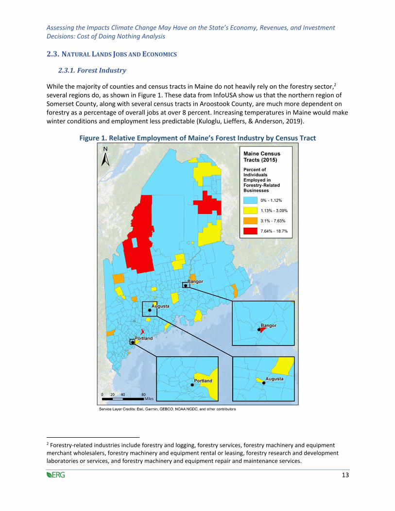
While the majority of counties and census tracts in Maine do not heavily rely on the forestry sector,2 several regions do, as shown in Figure 1. These data from InfoUSA show us that the northern region of Somerset County, along with several census tracts in Aroostook County, are much more dependent on forestry as a percentage of overall jobs at over 8 percent. Increasing temperatures in Maine would make winter conditions and employment less predictable (Kuloglu, Lieffers, & Anderson, 2019).
Figure 1. Relative Employment of Maine’s Forest Industry by Census Tract
2 Forestry-related industries include forestry and logging, forestry services, forestry machinery and equipment merchant wholesalers, forestry machinery and equipment rental or leasing, forestry research and development laboratories or services, and forestry machinery and equipment repair and maintenance services.
Assessing the Impacts Climate Change May Have on the State’s Economy, Revenues, and Investment Decisions: Cost of Doing Nothing Analysis
14
2.3.2. Agricultural Industry
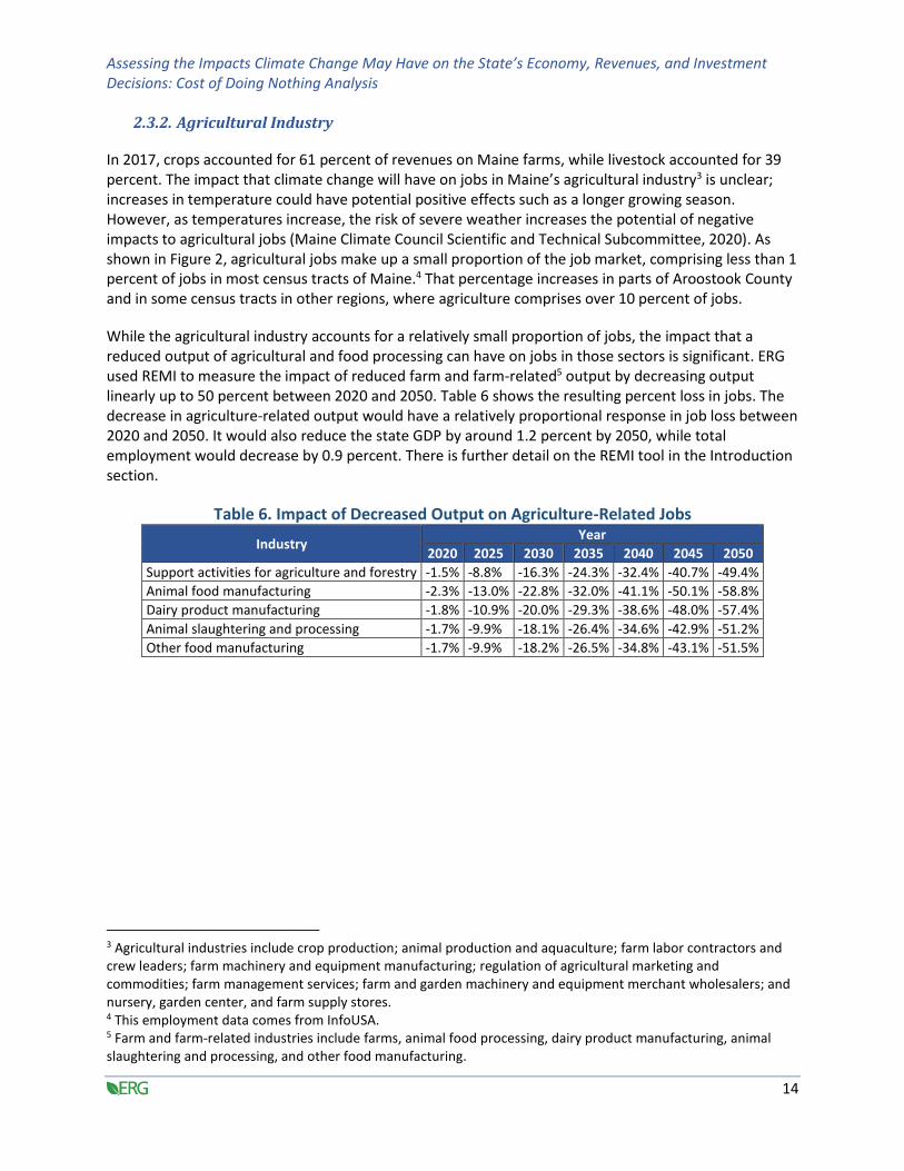
In 2017, crops accounted for 61 percent of revenues on Maine farms, while livestock accounted for 39 percent. The impact that climate change will have on jobs in Maine’s agricultural industry3 is unclear; increases in temperature could have potential positive effects such as a longer growing season. However, as temperatures increase, the risk of severe weather increases the potential of negative impacts to agricultural jobs (Maine Climate Council Scientific and Technical Subcommittee, 2020). As shown in Figure 2, agricultural jobs make up a small proportion of the job market, comprising less than 1 percent of jobs in most census tracts of Maine.4 That percentage increases in parts of Aroostook County and in some census tracts in other regions, where agriculture comprises over 10 percent of jobs.
While the agricultural industry accounts for a relatively small proportion of jobs, the impact that a reduced output of agricultural and food processing can have on jobs in those sectors is significant. ERG used REMI to measure the impact of reduced farm and farm-related5 output by decreasing output linearly up to 50 percent between 2020 and 2050. Table 6 shows the resulting percent loss in jobs. The decrease in agriculture-related output would have a relatively proportional response in job loss between 2020 and 2050. It would also reduce the state GDP by around 1.2 percent by 2050, while total employment would decrease by 0.9 percent. There is further detail on the REMI tool in the Introduction section.
Table 6. Impact of Decreased Output on Agriculture-Related Jobs
Industry Year
2020 2025 2030 2035 2040 2045 2050
Support activities for agriculture and forestry -1.5% -8.8% -16.3% -24.3% -32.4% -40.7% -49.4%
Animal food manufacturing -2.3% -13.0% -22.8% -32.0% -41.1% -50.1% -58.8%
Dairy product manufacturing -1.8% -10.9% -20.0% -29.3% -38.6% -48.0% -57.4%
Animal slaughtering and processing -1.7% -9.9% -18.1% -26.4% -34.6% -42.9% -51.2%
Other food manufacturing -1.7% -9.9% -18.2% -26.5% -34.8% -43.1% -51.5%
3 Agricultural industries include crop production; animal production and aquaculture; farm labor contractors and crew leaders; farm machinery and equipment manufacturing; regulation of agricultural marketing and commodities; farm management services; farm and garden machinery and equipment merchant wholesalers; and nursery, garden center, and farm supply stores. 4 This employment data comes from InfoUSA. 5 Farm and farm-related industries include farms, animal food processing, dairy product manufacturing, animal slaughtering and processing, and other food manufacturing.

Assessing the Impacts Climate Change May Have on the State’s Economy, Revenues, and Investment Decisions: Cost of Doing Nothing Analysis
15
Figure 2. Relative Employment in the Agricultural Industry by Census Tract
2.4. CLIMATE IMPACTS ON FORESTRY
Carbon sequestration in forests is exceedingly important to reduce greenhouse gases in Maine, sequestering over 60 percent of the state’s annual emissions (Maine Climate Council Scientific and Technical Subcommittee, 2020). Though land use changes may be the largest threat to this sequestration, other concerns exist for forests in Maine. Maine has high populations of non-native pests, many of which are increasing as a result of climate change. The ranges of both pests and native species are set to change with increased temperatures and unpredictable precipitation events (Maine Climate Council Scientific and Technical Subcommittee, 2020).

Assessing the Impacts Climate Change May Have on the State’s Economy, Revenues, and Investment Decisions: Cost of Doing Nothing Analysis
16
Maine’s average temperatures are set to increase at a greater rate than the national average (Maine Climate Council Scientific and Technical Subcommittee, 2020). These changes can impact the available wood supply and future composition of the forests. With expected warmer temperatures and less snow, spruce-fir forest types will likely decline along their southern habitat range, though they will likely be replaced by birch and maple species as more forests become mixed forest types (Janowiak et al., 2018). The overall productivity of forests is hard to predict because a longer growing season due to warmer temperatures will allow some species to thrive while others will decline (Maine Climate Council Scientific and Technical Subcommittee, 2020).
Winter harvesting benefits forests by providing a frozen forest floor, which decreases negative impacts on soils from heavy machinery (Kuloglu, Lieffers, & Anderson, 2019). However, rising temperatures will result in fewer frozen days, increasing the amount of labor and equipment needed to harvest the same amount of wood as a cold season. A modeling study in Alberta, Canada, demonstrated that the increased costs per cubic meter of wood harvest will increase 2.8 to 5.3 percent by 2050 if temperatures continue to rise, as the number of shutdown days due to warm temperatures increased (Kuloglu, Lieffers, & Anderson, 2019). Furthermore, interviews with loggers revealed that they compensate for shifting harvesting patterns by “overweighting” during transportation to the mill (Rittenhouse & Rissman, 2015). This practice can create unsafe road conditions or increase the need for road maintenance (Rittenhouse & Rissman, 2015). Though there are strong indications that doing nothing will negatively impact both harvesting and transportation, many stakeholders are still uncertain about additional effects, creating an increased financial risk for loggers that stay in the industry (Geisler, Rittenhouse, & Rissman, 2016).
2.5. CLIMATE IMPACTS ON AGRICULTURE
Carbon sequestration from agricultural lands will play a large role in addressing climate change in Maine and achieving the State’s goal of carbon neutrality in 2045. Protecting agricultural lands is key to carbon capture. However, pressing issues threaten agricultural production. The two main concerns related to climate change are an increased number of extreme precipitation events (≥ 2 inches of precipitation per day) and increased heat (Maine Climate Council Scientific and Technical Subcommittee, 2020). Though these climate changes could have some positive impacts, each will undoubtedly have negative effects as well.
Annual precipitation averages across seasons are expected to be mild in Maine compared to other states; however, the number of extreme precipitation events (≥2in/day) are expected to increase over time and pose significant threats to Maine’s agricultural industries (Maine Climate Council Scientific and Technical Subcommittee, 2020). Extreme precipitation events cause many negative impacts. While irrigation can assist farmers in drought conditions, draining excess water is more challenging. This increased moisture also threatens the number of field days that farmers can work and can cause shifts in the planting season, as well as crop loss through rotting seeds. It can also negatively impact livestock health (Maine Climate Council Scientific and Technical Subcommittee, 2020).
Increased heat will have several contrasting effects on agriculture in Maine. For example, the growing season has already begun to last longer, potentially increasing the growth and yield of some crops while negatively impacting others (Birkel & Mayewski, 2018). Rising temperatures could also require fewer heating costs but may counteract that benefit by requiring higher cooling costs. Finally, increased heat could lead to heat stress for workers, livestock, and crops (Wolfe, et al., 2018).
Assessing the Impacts Climate Change May Have on the State’s Economy, Revenues, and Investment Decisions: Cost of Doing Nothing Analysis
17
3. BLUE CARBON
3.1. INTRODUCTION
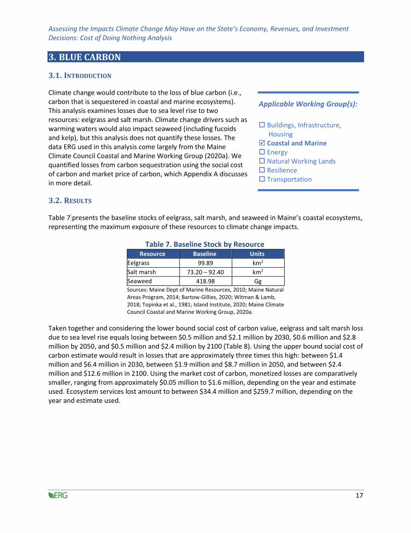
Climate change would contribute to the loss of blue carbon (i.e., carbon that is sequestered in coastal and marine ecosystems). This analysis examines losses due to sea level rise to two resources: eelgrass and salt marsh. Climate change drivers such as warming waters would also impact seaweed (including fucoids and kelp), but this analysis does not quantify these losses. The data ERG used in this analysis come largely from the Maine Climate Council Coastal and Marine Working Group (2020a). We quantified losses from carbon sequestration using the social cost of carbon and market price of carbon, which Appendix A discusses in more detail.
3.2. RESULTS
Table 7 presents the baseline stocks of eelgrass, salt marsh, and seaweed in Maine’s coastal ecosystems, representing the maximum exposure of these resources to climate change impacts.
Table 7. Baseline Stock by Resource Resource Baseline Units
Eelgrass 99.89 km2 Salt marsh 73.20 – 92.40 km2 Seaweed 418.98 Gg Sources: Maine Dept of Marine Resources, 2010; Maine Natural Areas Program, 2014; Bartow-Gillies, 2020; Witman & Lamb, 2018; Topinka et al., 1981; Island Institute, 2020; Maine Climate Council Coastal and Marine Working Group, 2020a.
Taken together and considering the lower bound social cost of carbon value, eelgrass and salt marsh loss due to sea level rise equals losing between $0.5 million and $2.1 million by 2030, $0.6 million and $2.8 million by 2050, and $0.5 million and $2.4 million by 2100 (Table 8). Using the upper bound social cost of carbon estimate would result in losses that are approximately three times this high: between $1.4 million and $6.4 million in 2030, between $1.9 million and $8.7 million in 2050, and between $2.4 million and $12.6 million in 2100. Using the market cost of carbon, monetized losses are comparatively smaller, ranging from approximately $0.05 million to $1.6 million, depending on the year and estimate used. Ecosystem services lost amount to between $34.4 million and $259.7 million, depending on the year and estimate used.
Applicable Working Group(s):
Buildings, Infrastructure,
Housing Coastal and Marine Energy Natural Working Lands Resilience Transportation

Assessing the Impacts Climate Change May Have on the State’s Economy, Revenues, and Investment Decisions: Cost of Doing Nothing Analysis
18
Table 8. Summary of Area Lost and Social Cost of CO2 Burial Loss (Eelgrass and Salt Marsh) Resource/
Year [a]
Sea Level Rise (ft)
Area Remaining (km2)
Area Lost (km2) Social Cost of Cumulative CO2 Burial Lost (2019$)
Market Cost of Cumulative CO2 Burial Lost (2019$)
Ecosystem Services
Low High Low [b] High [c] Low b] High [c] Low [d] High [e] Estimate A Estimate B
Eelgrass
Baseline Mean lower low water
(MLLW)
99.89 99.89 0.00 0.00 — — — — —
2030 MLLW + 1 97.17 94.33 2.72 5.56 $60,574 $217,925 $6,461 $23,243 $4,832,795 $4,832,795
2050 MLLW + 2 96.51 92.69 3.38 7.20 $103,876 $389,443 $14,953 $56,062 $8,732,102 $8,732,102
2100 MLLW + 4 94.33 87.90 5.56 11.99 $285,053 $1,081,891 $116,465 $442,031 $36,619,161 $36,619,161
Salt Marsh
Baseline — 73.20 92.40 0.00 0.00 — — — — — —
2030 HAT + 1.2 12.50 31.70 60.70 60.70 $392,614 $1,874,828 $41,875 $199,962 $99,544,106 $29,518,830
2050 HAT + 1.6 16.40 35.60 56.80 56.80 $500,386 $2,451,164 $72,033 $352,856 $135,440,265 $40,163,485
2100 HAT + 3.9 36.50 55.70 36.70 36.70 $478,627 $2,918,929 $195,554 $1,192,595 $223,098,693 $66,157,734
Total
2030 — 109.67 126.03 63.42 66.26 $453,188 $2,092,753 $48,335 $223,205 $104,376,901 $34,351,626
2050 — 112.91 128.29 60.18 64.00 $604,262 $2,840,606 $86,986 $408,918 $144,172,367 $48,895,587
2100 — 130.83 143.60 42.26 48.69 $763,680 $4,000,819 $312,019 $1,634,626 $259,717,854 $102,776,895
[a] Eelgrass and salt marsh response to sea level rise (ft) aligns with the time-based sea level rise projections described in the Introduction to this report.
[b] For eelgrass, the lower bound social cost estimate reflects the low area lost estimate and low social cost of carbon estimate. For salt marsh, it includes the low area remaining estimate, low area lost estimate, and low social cost of carbon estimate.
[c] For eelgrass, the higher bound social cost estimate reflects the high area lost estimate and low social cost of carbon estimate. For salt marsh, it includes the high area remaining estimate, high area lost estimate, and low social cost of carbon estimate.
[d] For eelgrass, the lower bound market cost estimate reflects the low area lost estimate and the point estimate for the market cost of carbon. For salt marsh, it includes the low area remaining estimate, low area lost estimate, and the point estimate for the market cost of carbon.
[e] For eelgrass, the higher bound market cost estimate reflects the high area lost estimate and the point estimate for the market cost of carbon. For salt marsh, it includes the high area remaining estimate, high area lost estimate, and the point estimate for the market cost of carbon.
Sources: Maine Dept of Marine Resources, 2010; Maine Natural Areas Program, 2014; Bartow-Gillies, 2020; McLeod et al., 2011; Drake et al., 2015; Roman et al., 1997; Kroeger et al., 2017; Interagency Working Group, 2016; Synergy Energy Economics, 2020; Costanza et al., 2008; NOAA OCM, NHDES, and ERG, 2016; Taylor, 2012; BEA, 2020; Maine Climate Council Coastal and Marine Working Group, 2020a.

Assessing the Impacts Climate Change May Have on the State’s Economy, Revenues, and Investment Decisions: Cost of Doing Nothing Analysis
19
3.3. METHODS
3.3.1. Data
This analysis primarily relies on data compiled by the Maine Climate Council Coastal and Marine Working Group (2020a),6 which draw on state agency resources, peer-reviewed journal articles, and other publicly available reports. The sections that follow detail these data and how ERG used them to produce the estimates shown in Section 3.2. We first discuss our data source for the social cost of CO2 and then discuss each coastal resource (eelgrass, salt marsh, and seaweed) in turn.
3.3.1.1. Cost of Carbon
We monetized eelgrass and salt marsh losses using both the social cost and market price of CO2. The values used for blue carbon in particular are described briefly below. For additional discussion on monetizing carbon, see Appendix A.
Social cost of carbon: The social cost of carbon values in this section are drawn from EPA’s 2016 Interagency Working Group lower bound (3 percent model average) estimates and converted to dollars per gigagram (Gg) for use in conjunction with the eelgrass and salt marsh estimates provided by the Maine Climate Council Working Group (see Table A-3 in Appendix A).
As discussed in Appendix A, the Interagency Working Group (2016) also provides a higher bound, 95th percentile estimate for the social cost of carbon, which is approximately three times as high. The tables that follow do not show the results of the blue carbon analysis using this 95th percentile estimate, but those results are mentioned in the text.
Table 9. Lower Bound Social Cost of CO2 Used in Blue Carbon Analysis
Year 2007$/Metric Ton 2007–2019 Multiplier 2019$/Metric Ton 2019$/Gg
2030 $50.00 1.21 $60.74 $60,736.22
2050 $69.00 1.21 $83.82 $83,815.98
2100 $115.11 1.21 $139.82 $139,823.45 Sources: Interagency Working Group on Social Cost of Greenhouse Gases, 2016; BEA, 2020.
Market price of carbon: The market price of carbon uses estimates that Synergy Energy Economics (2020) developed for Maine based on ICF’s (2018) Regional Greenhouse Gas Initiative price forecast (see Appendix A for more details) converted to dollars per Gg.
Table 10. Market Price of CO2
Year 2018$/Short Ton 2019$-2018$ Multiplier 2019$/Short Ton 2019$/Gg
2030 $5.78 $1.02 $5.88 $6,477.88
2050 $10.76 $1.02 $10.95 $12,065.68
2100 $50.94 $1.02 $51.83 $57,128.05 Sources: Synapse Energy Economics (2020) based on ICF (2018).
6 The Maine Climate Council Coastal and Marine Working Group compiled their data in the “MCC CMWG DATA NEEDS” spreadsheet.

Assessing the Impacts Climate Change May Have on the State’s Economy, Revenues, and Investment Decisions: Cost of Doing Nothing Analysis
20
3.3.1.2. Ecosystem Services
“Ecosystem services” are the services provided by ecosystems and their associated species that help sustain and fulfill human life, either directly or indirectly—including both tangible and intangible services such as food, clean water and air, flood control, aesthetic beauty, or recreational opportunities (NOAA OCM, NHCP, and ERG 2016; Troy, 2012). These services can be monetized to capture the value they add. For eelgrass and seaweed, ERG includes values for the services that have been previously monetized (although this is unlikely to represent a comprehensive valuation of the services provided).
For eelgrass, we sum estimates for two services from a National Oceanic and Atmospheric Administration Office for Coastal Management (NOAA OCM), New Hampshire Department of Environmental Services Coastal Program (NHCP), and ERG (2016) report:
• Commercial fishing (eelgrass provides nursery habitat and forage area for commercially fished species, and as warming waters reduce eelgrass stocks, the commercial fish landings will be reduced).
• Nitrogen removal (eelgrass reduces the amount of nitrogen in the water column, leading to reduced expenditures for wastewater treatment by neighboring towns).
The eelgrass commercial fishing estimate is drawn from the NOAA OCM, NCHP, and ERG (2016) analysis of the ecosystem services provided by New Hampshire’s Great Bay Estuary. Using a “trophic transfer” approach that starts with the primary productivity of the ecosystem, the estimate calculates the amount lost in successively higher parts of the food chain. It begins with an estimate that benthic faunal production of eelgrass is 175 grams of dry weight per m2 per year, equivalent to 708.2005 kg of dry weight per acre per year. Assuming dry weight is 22 percent of wet weight yields approximately 3,219.09 kg wet weight per acre per year. Of this, 4 percent is estimated to remain in the tropic level associated with commercially fished species, yielding approximately 128.8 kg wet weight per acre per year (3,219.09 × 0.04). ERG monetized this estimate using landings and total revenue data for New Hampshire by species for 2010–2014, which resulted in a value of $4.64 per kg. Multiplying the 128.8 kg wet weight per acre per year estimate by $4.64 per kg yields approximately $598 per acre per year (in 2015 dollars). For this analysis, we convert that estimate to a dollar per km2 value and inflate from 2015 dollars to 2019 dollars using the Bureau of Economic Analysis’ (BEA’s) (2020) implicit price deflator for GDP, resulting in an estimate of $158,432 per km2 per year in 2019.
The eelgrass nitrogen removal estimate is also drawn from the NOAA OCM, NCHP, and ERG (2016) analysis. That estimate is based on Cole and Moksnes’ (2016) estimate that eelgrass removes 12.3 kg of nitrogen per hectare per year, or 67 pounds of nitrogen per acre per year. We monetized this nitrogen removal using a NOAA Regional Ecosystem Services Research Program (2015) estimate of $68 to $77 per pound in the Great Bay Estuary. For this estimate, we use the midpoint of those two estimates: $72.50, resulting in approximately $4,858 per acre per year in 2015 dollars (67 × $72.50). Converting to a dollar per km2 value and inflating from 2015 dollars to 2019 dollars using the BEA’s (2020) implicit price deflator for GDP results in a value of $1,287,722 per km2 per year in 2019.
For salt marsh, we use two partially overlapping estimates. Estimate A combines three estimates from two sources (NOAA OCM, NCHP, and ERG, 2016; Costanza, 2008) and includes:

Assessing the Impacts Climate Change May Have on the State’s Economy, Revenues, and Investment Decisions: Cost of Doing Nothing Analysis
21
• Commercial fishing (salt marsh provides nursery habitat and forage area for commercially fished species, and as warming waters reduce eelgrass stocks, the commercial fish landings will be reduced).
• Nitrogen removal (salt marsh reduces the amount of nitrogen in the water column, leading to reduced expenditures for wastewater treatment by neighboring towns).
• Hurricane protection (salt marsh and other coastal wetlands reduce hurricane damages in coastal areas).
Estimate B comes from one source (Troy, 2012) and includes several services for coastal/saltwater wetlands:
• Aesthetic and amenity
• Disturbance regulation
• Gas/atmospheric regulation
• Habitat refugium
• “Other cultural”
• Recreation
The salt marsh commercial fishing value used in Estimate A is drawn from the NOAA OCM, NCHP, and ERG (2016) analysis. It begins with an estimate that the primary productivity of marsh grasses is 500 grams of dry weight per m2 per year in New England marshes, and benthic microalgal production is 106 grams of dry weight per square m2 per year, for a total of 606 grams of dry weight per m2 per year, or 2,452,397 grams of dry weight per acre per year. Assuming dry weight is 22 percent of wet weight yields approximately 11,147 kg wet weight per acre per year. Only 0.16 percent of this productivity is estimated to remain in the tropic level associated with commercially fished species, yielding approximately 17.8 kg wet weight per acre per year (11,147 × 0.016). As with the eelgrass commercial fishing estimate, a value of $4.64 per kg is applied, resulting in approximately $82 per acre per year (in 2015 dollars). For this analysis, we convert that estimate to a dollar per km2 value and inflate from 2015 dollars to 2019 dollars using the BEA’s (2020) implicit price deflator for GDP, resulting in an estimate of $21,895 per km2 per year in 2019.
The salt marsh nitrogen removal value used in Estimate A is also drawn from the NOAA OCM, NCHP, and ERG (2016) analysis. That estimate is based on Drake et al.’s (2015) finding that salt marsh in the Rachel Carson National Wildlife Refuge in Maine and Parker River National Wildlife Refuge in Massachusetts removes between 2.8 and 11.3 grams of nitrogen per m2 per year, or between 25 and 101 pounds of nitrogen per acre per year. The NOAA OCM, NCHP, and ERG (2016) analysis uses the midpoint of that range: 63 pounds of nitrogen per acre per year. As with eelgrass, we monetized nitrogen removal using the midpoint—$72.50—of the NOAA Regional Ecosystem Services Research Program’s (2015) estimate of $68 to $77 per pound in the Great Bay Estuary. This results in approximately $4,568 per acre per year in 2015 dollars (63 × $72.50). Converting to a dollar per km2 value and inflating from 2015 dollars to 2019 dollars using the BEA’s (2020) implicit price deflator for GDP results in a value of $1,210,843 per km2 per year in 2019.
Assessing the Impacts Climate Change May Have on the State’s Economy, Revenues, and Investment Decisions: Cost of Doing Nothing Analysis
22
The salt marsh hurricane protection value used in Estimate A is drawn from Costanza et al.’s (2008) regression model of the value of coastal wetlands for hurricane protection for U.S. states. By comparing the damage from major hurricanes that hit the Atlantic and Gulf coasts between 1980 and 2004 with the coastal wetland area in each storm’s swath, Costanza et al. (2008) calculated a hurricane protection value of $770.10 per hectare per year for Maine (in 2004 dollars). Converting to a dollar per km2 value and inflating from 2015 dollars to 2019 dollars using the BEA’s (2020) implicit price deflator for GDP results in a value of $102,049 per km2 per year in 2019.
The aggregated salt/coastal wetlands value used in Estimate B is drawn from Troy’s (2012) ecosystem service valuation for Maine and includes several ecosystem services:
• Aesthetic and amenity ($436 per acre per year in 2011 dollars)
• Disturbance regulation ($371 per acre per year in 2011 dollars)
• Gas/atmospheric regulation ($5 per acre per year in 2011 dollars)
• Habitat refugium ($117 per acre per year in 2011 dollars)
• “Other cultural” ($20 per acre per year in 2011 dollars)
• Recreation ($450 per acre per year in 2011 dollars)
Summing these values results in a total of $1,399 per acre per year in 2011 dollars. Converting to a dollar per km2 value and inflating from 2015 dollars to 2019 dollars using the BEA’s (2020) implicit price deflator for GDP results in a value of $395,818 per km2 per year in 2019.
We projected the value of these ecosystem services in future years (2030, 2050, and 2100) using the average annual increase in the BEA’s (2020) implicit price deflator for GDP, 1.89 percent.
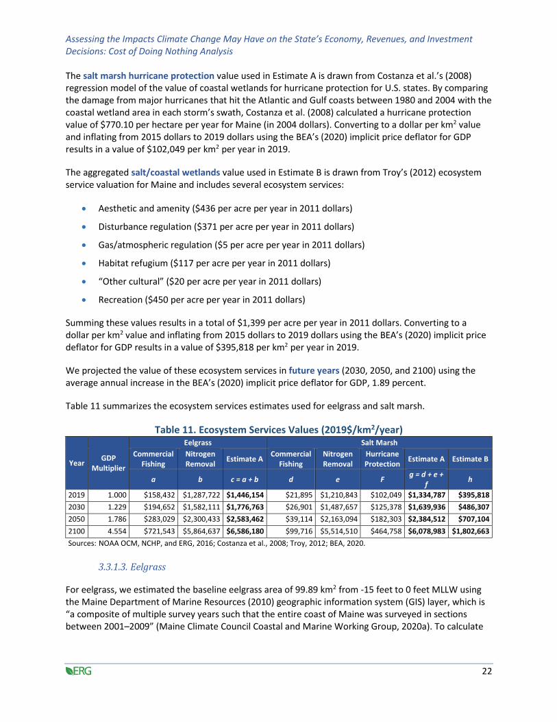
Table 11 summarizes the ecosystem services estimates used for eelgrass and salt marsh.
Table 11. Ecosystem Services Values (2019$/km2/year)
Year GDP
Multiplier
Eelgrass Salt Marsh
Commercial Fishing
Nitrogen Removal
Estimate A Commercial
Fishing Nitrogen Removal
Hurricane Protection
Estimate A Estimate B
a b c = a + b d e F g = d + e +
f h
2019 1.000 $158,432 $1,287,722 $1,446,154 $21,895 $1,210,843 $102,049 $1,334,787 $395,818
2030 1.229 $194,652 $1,582,111 $1,776,763 $26,901 $1,487,657 $125,378 $1,639,936 $486,307
2050 1.786 $283,029 $2,300,433 $2,583,462 $39,114 $2,163,094 $182,303 $2,384,512 $707,104
2100 4.554 $721,543 $5,864,637 $6,586,180 $99,716 $5,514,510 $464,758 $6,078,983 $1,802,663
Sources: NOAA OCM, NCHP, and ERG, 2016; Costanza et al., 2008; Troy, 2012; BEA, 2020.
3.3.1.3. Eelgrass
For eelgrass, we estimated the baseline eelgrass area of 99.89 km2 from -15 feet to 0 feet MLLW using the Maine Department of Marine Resources (2010) geographic information system (GIS) layer, which is “a composite of multiple survey years such that the entire coast of Maine was surveyed in sections between 2001–2009” (Maine Climate Council Coastal and Marine Working Group, 2020a). To calculate

Assessing the Impacts Climate Change May Have on the State’s Economy, Revenues, and Investment Decisions: Cost of Doing Nothing Analysis
23
the area lost, we used low and high estimates based on a vertical depth uncertainty of 3.28 feet.7 Table 12 shows the baseline area, estimated area lost to sea level rise by year, remaining area, and percentage of the baseline area lost.
Table 12. Eelgrass—Baseline Area, Area Lost, and Area Remaining by Year
Year Sea
Level Rise (ft)
Baseline Area (km2)
Area Lost (km2) Area Remaining (km2) % Area Lost
Low Loss High Loss Low Loss High Loss Low Loss High Loss
a B c d = a - b e = a - c f = b ÷ a g = c ÷ a
Baseline 0 99.89 0.00 0.00 99.89 99.89 0.0% 0.0%
2030 1 99.89 2.72 5.56 97.17 94.33 2.7% 5.6%
2050 2 99.89 3.38 7.20 96.51 92.69 3.4% 7.2%
2100 4 99.89 5.56 11.99 94.33 87.90 5.6% 12.0%
Sources: Maine Dept of Marine Resources, 2010; Maine Climate Council Coastal and Marine Working Group, 2020a.
Table 13 shows the amount of eelgrass-related carbon burial lost by year. We estimated carbon burial rates using data from McLeod et al. (2011), which presents low and high burial estimates based on the mean of 138 grams of carbon (gC)/m2/year with a standard error of ± 38. Carbon is converted to equivalent CO2 using a factor of 44/12.8 We calculated the burial amount lost by multiplying the low and high amounts of eelgrass area lost by the low and high carbon sequestration rates and carbon to CO2 conversion factor, then dividing by 1,000 to yield Gg CO2 equivalent amount lost per year.
Table 13. Eelgrass—Carbon Burial Lost by Year
Year
Carbon Sequestration Rates (gC/m2/Year)
C to CO2 Equivalent Conversion
Burial Amount Lost (Gg CO2 Equivalent/Year)
Low Burial High Burial Low Burial High Burial
Low Loss High Loss Low Loss High Loss
h i j k = (b × h × j)
÷ 1,000 l = (c × h × j) ÷
1,000
m = (b × i × j)
÷ 1,000 n = (c × i × j) ÷
1,000
Baseline 100 176 3.6667 0.000 0.000 0.000 0.000
2030 100 176 3.6667 0.997 2.039 1.755 3.588
2050 100 176 3.6667 1.239 2.640 2.181 4.646
2100 100 176 3.6667 2.039 4.396 3.588 7.738 Sources: Maine Dept of Marine Resources, 2010; McLeod et al., 2011; Maine Climate Council Coastal and Marine Working Group, 2020a.
To monetize the burial amount lost, we multiplied the amount lost from each of the four burial/loss scenarios (from Table 13) by the low-bound social cost and the market price of CO2 in each year (from Table 9 and Table 10) (with the results shown in Table 14). Using the upper bound social cost of carbon estimate results in values that are approximately three times as high as those shown in Table 14, ranging from approximately $0.2 million to $3.4 million depending on the year and low/burial estimates used. Appendix A provides more information on the high- and low-bound social cost of carbon estimates.
7 This estimate was rounded to 100 km2 in the “MCC CMWG DATA NEEDS” spreadsheet; we use the unrounded figure here. 8 This estimate was rounded to either 3.666 or 3.66 in the “MCC CMWG DATA NEEDS” spreadsheet; we use the unrounded figure here.

Assessing the Impacts Climate Change May Have on the State’s Economy, Revenues, and Investment Decisions: Cost of Doing Nothing Analysis
24
Table 14. Eelgrass—Social and Market Cost of CO2 Burial Lost (2019$)
Year
Cost of CO2 per Gg (2019$)
Cost of CO2 Burial Lost (2019$)
Low Burial High Burial
Low Loss High Loss Low Loss High Loss
o p = k × o q = l × o r = m × o s = n × p
Low-Bound Social Cost
2030 $60,736 $60,574 $123,821 $106,611 $217,925
2050 $83,816 $103,876 $221,274 $182,822 $389,443
2100 $139,823 $285,053 $614,711 $501,694 $1,081,891
Market Price
2030 $6,478 $6,461 $13,206 $11,371 $23,243
2050 $12,066 $14,953 $31,853 $26,318 $56,062
2100 $57,128 $116,465 $251,154 $204,978 $442,031 Sources: Maine Dept of Marine Resources, 2010; McLeod et al., 2011; Interagency Working Group, 2016; Synergy Energy Economics, 2020; BEA, 2020; Maine Climate Council Coastal and Marine Working Group, 2020a.
To estimate the ecosystems services value lost, we multiply the ecosystems services value in each year (from Table 11) by the eelgrass area lost under each sea level rise scenario (from Table 12). This results in values between $4.8 million and $79.0 million (see Table 15).
Table 15. Eelgrass—Ecosystems Services Lost (2019$)
Year
Ecosystems Services Value (2019$)
Cost of Ecosystems Services Lost (2019$)
Low Loss High Loss
t u = b × t v = c × t
2030 $1,776,763 $4,832,795 $9,878,802
2050 $2,583,462 $8,732,102 $18,600,927
2100 $6,586,180 $36,619,161 $78,968,299 Sources: Maine Dept of Marine Resources, 2010; McLeod et al., 2011; NOAA OCM, NCHP, and ERG, 2016; BEA, 2020; Maine Climate Council Coastal and Marine Working Group, 2020a.
3.3.1.4. Salt Marsh
The salt marsh analysis reflects several conflicting influences on the ability of salt marsh to sequester CO2:
• The ability of healthy salt marsh to sequester CO2
• Loss of salt marsh area due to sea level rise (which reduces CO2 sequestration)
• Tidal marsh restrictions (which reduce CO2 sequestration)
• Tidal marsh restrictions (which also increase methane emissions)
We used tidal marsh mapping data on baseline salt marsh area from the Maine Natural Areas Program (2014). We only included salt and brackish marsh (because freshwater marsh does not have the same CO2/methane sequestration and emissions potential). The low area estimate includes the initial Maine Natural Areas Program mapping effort, which did not attempt to map areas smaller than a certain acreage or fringing marshes. The high area estimate is drawn from the Maine Coastal Program (Bartow-Gillies, 2020) desktop analysis of all coastal marshes using the National Wetland Inventory, aerial images, and other GIS tools, and it includes marshes of all sizes and types.

Assessing the Impacts Climate Change May Have on the State’s Economy, Revenues, and Investment Decisions: Cost of Doing Nothing Analysis
25
The estimate of the area lost due to sea level rise is based on the Maine Natural Areas Program marsh migration model, with the assumption that “no current marsh habitat will keep pace with sea level rise (i.e., that they will not accrete enough sediment with sea level rise to maintain vegetation), and only new marsh will be formed at higher elevations” (Maine Climate Council Coastal and Marine Working Group, 2020a).
Table 16 summarizes the baseline area, area lost under each sea level rise scenario, area remaining, and percentage of area lost to sea level rise. Note that salt marshes experience sudden and major loss under the 2030–1.2-foot sea level rise scenario but then start to slowly regain ground in future years. This modeling result is because marshes may migrate as additional sea level rise reaches areas of low flatlands, wetlands, and creeks where marshes have more potential for lateral expansion. If these modeling assumptions hold, then the majority of salt marsh losses will occur in the next 10 years, making near-term marsh adaptation maximally effective.
Table 16. Salt Marsh—Baseline Area, Area Lost, and Area Remaining by Year
Year
Sea Level
Rise (ft)
Baseline Area (km2) Area Lost (km2)
Area Remaining (km2) % Area Lost
Low Area High Area Low Area High Area Low Area High Area
a b c d = a - b e = b - c f = c ÷ a f = c ÷ b
Baseline 0.0 73.2 92.4 0.0 73.2 92.4 0.0% 0.0%
2030 1.2 73.2 92.4 60.7 12.5 31.7 82.9% 65.7%
2050 1.6 73.2 92.4 56.8 16.4 35.6 77.6% 61.5%
2100 3.9 73.2 92.4 36.7 36.5 55.7 50.1% 39.7% Sources: Maine Natural Areas Program, 2014; Bartow-Gillies, 2020; Maine Climate Council Coastal and Marine Working Group, 2020a.
In marshes where a road or other crossing restricts the full tidal flow and cycle, carbon sequestration is significantly reduced, and restricted marshes can become net methane emitters when they have salinity less than 18 parts per thousand (ppt.) Tidal flow crossings that can cause restrictions include culverts, bridges, dams, dikes, causeways, road grades, railroad grades, trails, and dirt roads. The Maine Coastal Program estimated the number of current and future tidal marsh crossings using the Maine Natural Areas Program marsh migration scenarios as well as modeling of where future marsh migration areas and the corridors to those areas would cross culverts, bridges, dams, etc.
The percentage of tidal marsh crossings that restrict flows is based on a desktop analysis of current conditions, with restriction assessed based on the presence of upstream or downstream scour, different vegetation community type, or culvert perch (Bartow-Gillies, 2020). This analysis suggests that between 336 and 347 of 368 crossings (91 to 94 percent) are restrictive. These same percentages are assumed to hold in the future as well. Multiplying the number of tidal marsh crossings in future years by the percentage that restrict tidal flow yields the number of tidal marsh crossing restrictions in future years (see Table 17).
To estimate methane emissions due to tidal crossing restrictions, we calculated the current level of methane emissions due to restrictions by dividing the point estimate, 39.1 km2, by the low and high marsh area from Table 16 and then averaged those percentages. This results in an estimate of
approximately 48 percent, which is assumed to hold in future years (39.1 ÷ 73.2 = 53 percent, and 39.1

Assessing the Impacts Climate Change May Have on the State’s Economy, Revenues, and Investment Decisions: Cost of Doing Nothing Analysis
26
÷ 92.4 = 42 percent; the average of 53 percent and 42 percent is 48 percent).9 (This estimate assumes that the tidal restrictions cause the marshes to have salinities of less than 18 ppt.) We then multiplied this percentage by the low and high remaining marsh area to estimate methane emissions in each future scenario (see Table 17).
Table 17. Salt Marsh—Methane (CH4) Emissions Due to Tidal Marsh Crossing Restrictions
Year
Number of Tidal Marsh
Crossings
Baseline % Tidal Marsh Crossings
Restricting Tidal Flow
Number of Tidal Marsh Crossing
Restrictions
Average CH4 Emissions per Marsh Area
(km2)
CH4 Emissions Due to Restrictions (km2)
Low High Low High Low High Low Area High Area
g h i j k = g × i l = h × j m = ((n ÷ a) +
(o ÷ b)) ÷ 2 n = m × d o = m × e
Baseline 368 368 91.3% 94.3% 336 347 47.87% 39.100 39.100
2030 534 545 91.3% 94.3% 488 514 47.87% 5.983 15.173
2050 542 553 91.3% 94.3% 495 521 47.87% 7.850 17.040
2100 619 630 91.3% 94.3% 565 594 47.87% 17.471 26.661 Sources: Maine Natural Areas Program, 2014; Bartow-Gillies, 2020; Maine Climate Council Coastal and Marine Working Group, 2020a.
Table 18 shows the estimates used to calculate sequestration, emissions due to methanogenesis, and to convert carbon to CO2 equivalent. The low sequestration estimate is drawn from Drake et al. (2015), and the high value from Roman et al. (1997). For emissions due to methanogenesis, both the low and high values are drawn from Kroeger et al. (2017). Carbon is converted to equivalent CO2 using a factor of 44/12.10
Table 18. Salt Marsh—Emissions Factors and Carbon to CO2 Equivalent Conversion
Year
Emissions Factors Used in the Carbon Burial Calculations C to CO2 Equivalent
Conversion C Sequestration (gC/m2-yr) C Emissions (Methanogenesis)
Low High Low High
p q r s t
Baseline -74 -256 8.4 41.6 3.6667
2030 -74 -256 8.4 41.6 3.6667
2050 -74 -256 8.4 41.6 3.6667
2100 -74 -256 8.4 41.6 3.6667 Sources: Drake et al., 2015; Roman et al., 1997; Kroeger et al., 2017; Maine Climate Council Coastal and Marine Working Group, 2020a.
Table 19 estimates sequestration, emissions due to tidal restrictions, and emissions due to methanogenesis, sums these to calculate net carbon burial, and calculates the loss of carbon burial by
finding the change (Δ) in each future year from the baseline. Four scenarios are calculated by combining the low and high burial estimates (from Table 18) with the low and high marsh area remaining estimates (from Table 16) and the sequestration and emissions factors (from Table 17).
9 Note that while this estimate was rounded to 48.0 percent in the “MCC CMWG DATA NEEDS” spreadsheet, we use the unrounded figure here. 10 Note that while this estimate was rounded to either 3.666 or 3.66 in the “MCC CMWG DATA NEEDS” spreadsheet, we use the unrounded figure here.

Assessing the Impacts Climate Change May Have on the State’s Economy, Revenues, and Investment Decisions: Cost of Doing Nothing Analysis
27
Table 19. Salt Marsh—Net Carbon Burial (Gg CO2 Equivalent/Year)
Year Sequestration Emissions
(Restrictions) Emissions
(Methanogenesis) Net Lost
Low Burial Amount/Low Marsh Area Scenario
u = (d × p × t) ÷ 1,000 v = (n × p × t) ÷ 1,000 w = (n × r × t) ÷ 1,000 x = u + v + w y = Δ(x)
Baseline -19.86 10.61 1.20 -8.05 0.00
2030 -3.39 1.62 0.18 -1.58 6.46
2050 -4.45 2.13 0.24 -2.08 5.97
2100 -9.90 4.74 0.54 -4.63 3.42
Low Burial Amount/High Marsh Area Scenario
z = (e × p × t) ÷ 1,000 aa = (o × p × t) ÷ 1,000 ab = (o × r × t) ÷ 1,000 ac = y + z + aa ad = Δ(ac)
Baseline -25.07 10.61 1.20 -13.26 0.00
2030 -8.60 4.12 0.47 -4.02 9.24
2050 -9.66 4.62 0.52 -4.51 8.75
2100 -15.11 7.23 0.82 -7.06 6.20
High Burial Amount/Low Marsh Area Scenario
ae = (d × q × t) ÷ 1,000 af = (n × q × t) ÷ 1,000 ag = (n × s × t) ÷ 1,000 ah = ac + ad + ae ai= Δ(ah)
Baseline -68.71 36.70 5.96 -26.04 0.00
2030 -11.73 5.62 0.91 -5.20 20.84
2050 -15.39 7.37 1.20 -6.83 19.22
2100 -34.26 16.40 2.66 -15.20 10.85
High Marsh Area/High Burial Amount Scenario
aj = (e × q × t) ÷ 1,000 ak = (o × q × t) ÷ 1,000 al = (o × s × t) ÷ 1,000 am = ag + ah + ai an = Δ(am)
Baseline -86.73 36.70 5.96 -13.26 0.00
2030 -29.76 14.24 2.31 -4.02 30.87
2050 -33.42 16.00 2.60 -4.51 29.24
2100 -52.28 25.03 4.07 -7.06 20.88 Sources: Drake et al., 2015; Roman et al., 1997; Kroeger et al., 2017; Maine Climate Council Coastal and Marine Working Group, 2020a.
The final step for salt marsh is to calculate the social cost of CO2 burial lost by multiplying the low-bound social cost and market price (from Table 9 and Table 10) by the lost burial amounts in each of the four scenarios (from Table 19) (with the results shown in Table 20). Using the upper bound social cost of carbon estimate would result in values that are approximately three times as high as those shown in Table 20, ranging from approximately $1.2 million to $9.2 million, depending on the year and marsh area estimate used.

Assessing the Impacts Climate Change May Have on the State’s Economy, Revenues, and Investment Decisions: Cost of Doing Nothing Analysis
28
Table 20. Salt Marsh—Social and Market Cost of CO2 Burial Lost (2019$)
Year
Cost of CO2 per Gg (2019$)
Low Burial Amount Scenario (Gg CO2 Equivalent/Year)
High Burial Amount Scenario (Gg CO2 Equivalent/Year)
Low Marsh Area High Marsh Area Low Marsh Area High Marsh Area
ao ap = y × ao aq = ad × ao ar = ai × ao as = an × ao
Low-Bound Social Cost
2030 $60,736 $392,614 $561,258 $1,265,744 $1,874,828
2050 $83,816 $500,386 $733,115 $1,610,627 $2,451,164
2100 $139,823 $478,627 $866,870 $1,516,730 $2,918,929
Market Price
2030 $6,478 $41,875 $59,862 $134,999 $199,962
2050 $12,066 $72,033 $105,535 $231,857 $352,856
2100 $57,128 $195,554 $354,180 $619,694 $1,192,595 Sources: Drake et al., 2015; Roman et al., 1997; Kroeger et al., 2017; Interagency Working Group, 2016; Synergy Energy Economics, 2020; BEA, 2020; Maine Climate Council Coastal and Marine Working Group, 2020a.
To estimate the ecosystems services value lost, we multiply the ecosystems services value in each year (from Table 11) by the salt marsh area lost under each sea level rise scenario (from Table 16). This results in values between $4.8 million and $79.0 million (see Table 21).
Table 21. Salt Marsh—Ecosystems Services Lost (2019$)
Year Ecosystems Services Value (2019$) Cost of Ecosystems Services Lost (2019$)
at au = c × at
Ecosystems Services Estimate A
2030 $1,639,936 $99,544,106
2050 $2,384,512 $135,440,265
2100 $6,078,983 $223,098,693
Ecosystems Services Estimate B
2030 $486,307 $29,518,830
2050 $707,104 $40,163,485
2100 $1,802,663 $66,157,734 Sources: Maine Dept of Marine Resources, 2010; McLeod et al., 2011; Costanza et al., 2008; NOAA OCM, NCHP, and ERG, 2016; Troy, 2012; BEA, 2020; Maine Climate Council Coastal and Marine Working Group, 2020a.
3.3.1.5. Seaweed
For seaweed, we did not calculate the amount lost due to a lack of data availability. Table 22 shows the estimated baseline stock of different categories of seaweed in Maine. The Maine Climate Council Coastal and Marine Working Group estimated wild intertidal seaweed stocks (fucoids) by multiplying 50 fresh kg/m (Topinka, 1981) by the length of the coastline (8,047 km) and then by 1,000 to convert km to m. Wild subtidal seaweed (including sugar kelp, horsetail kelp, and shotgun kelp) is estimated by multiplying 2.05 fresh kg/m (a rough estimate using the average for Cashes Ledge) (Witman, 2018) by the length of the coastline (8,047 km) and then by 1,000 to convert km to m. We took the estimate of farmed subtidal seaweed (kelp)—325,000 pounds per year—from the Island Institute (2020) report and then converted it to kg. We then converted each of these to Gg of carbon using the Maine Climate Council Coastal and Marine Working Group’s estimate that 30 percent of seaweed is carbon.

Assessing the Impacts Climate Change May Have on the State’s Economy, Revenues, and Investment Decisions: Cost of Doing Nothing Analysis
29
Table 22. Seaweed—Baseline Stocks
Type Seaweed Stocks (kg) % of Seaweed = C Seaweed Stocks (Gg C)
Wild Intertidal Seaweed (Fucoids) 402,350,000 30% 181.06
Wild Subtidal Seaweed 16,477,956 30% 7.42
Farmed Subtidal Seaweed 147,418 30% 0.07
Total 418,975,374 30% 188.54 Sources: Witman & Lamb, 2018; Topinka et al., 1981; Island Institute, 2020; Maine Climate Council Coastal and Marine Working Group, 2020a.
Although we did not quantify seaweed losses due to a lack of data, the stock could conceptually increase due to increases in farmed edible seaweed and decrease due to rising temperatures. The Island Institute (2020) report estimates that the current level of farmed seaweed (147,418 kg) could increase to between 698,532 and 2,705,678 kg by 2035, with a best estimate of 1,387,993 kg.
The Maine Climate Council Coastal and Marine Working Group also estimates that the percentage of farmed and natural annual biomass production contributing to carbon sequestration in seaweed is between 4.30 and 18.89 percent, with a mean estimate of 10.92 percent (based on the mean and standard error presented in Krause-Jensen and Duarte [2016]).
3.3.2. Assumptions
This section notes the assumptions that the analysis used for each coastal resource, as specified by the Maine Climate Council Coastal and Marine Working Group (some of which have been mentioned already in Section 3.3.1).
3.3.2.1. Eelgrass
The Maine Climate Council Coastal and Marine Working Group assumes the following for eelgrass:
• The Maine Department of Marine Resources 2010 GIS layer is the best possible estimate of eelgrass area coastwide. More recent eelgrass area calculations are possible for Casco Bay (2018), Belfast Bay/Northport (2019), and the Piscataqua River/Portsmouth Harbor (2019). However, because eelgrass beds inherently expand and contract from year to year due to a multitude of factors (sea level rise, water quality, light availability, macroalgal competition, invasive species, fouling organisms, ice scour, vessel and mooring impacts, etc.) and the 2010 baseline survey is a composite of 2001–2009 surveys that includes the entire coast of Maine, the GIS layer is considered the best possible estimate of eelgrass area coastwide.
• The deep edge of Maine eelgrass beds is set at -15 feet MLLW based on the Maine Department of Marine Resources’ 2010 eelgrass layer and the NOAA Coastal Relief Model bathymetry raster, which demonstrated that approximately 98 percent of Maine's eelgrass resides shallower than or at -15 feet MLLW. Because light availability generally controls the deep edge of eelgrass, even a 1-foot increase in sea level could decrease light availability and cause beds residing several feet shallower than -15 feet MLLW to recede. Therefore, eelgrass losses caused by sea level rise could possibly be greater than those shown in Section 3.3.1.2 for nearer-term predictions (2030–2050 timeframe).
• The low and high area lost estimates are based on a vertical depth uncertainty of 3.28 feet (1 standard deviation) due to variation in actual water depth. This magnitude of vertical uncertainty overwhelms the sea level rise scenarios that are less than 3.28 feet, so instead of

Assessing the Impacts Climate Change May Have on the State’s Economy, Revenues, and Investment Decisions: Cost of Doing Nothing Analysis
30
providing a single value of loss for each specific sea level rise scenario, we provide a range of eelgrass areas vulnerable to each foot of sea level rise.
• Long-term burial rates assume that all eelgrass beds are equally healthy and equally capable of carbon sequestration. In reality, a range of burial rates is necessary, covering both highly functioning and/or long-present eelgrass beds as well as those that are more ephemeral and/or provide limited sequestration due to poor health.
3.3.2.2. Salt Marsh
The Maine Climate Council Coastal and Marine Working Group assumes the following for salt marsh:
• No current marshes will keep pace with sea level rise by accreting sediment. In all marsh migration scenarios, marsh area experiences a net loss compared to current 2020 conditions. This is based on the assumption that no current marshes will accrete sediment at a pace that maintains the elevation of salt marshes relative to the tidal flooding and duration necessary to maintain vegetated communities on marsh platforms.
• The analysis only includes salt and brackish marsh because freshwater marsh area does not have the same sequestration and emissions potential.
• Marsh area lost due to sea level rise is based on a "bathtub" GIS model using sea level rise scenarios to predict future areas where elevation could support marsh habitat. These scenarios assume that no current marsh habitat will keep pace with sea level rise (i.e., the habitat will not accrete enough sediment to maintain vegetation), and only new marsh will be formed at higher elevations. This model is not based on NOAA’s Sea Level Affecting Marshes Model (SLAMM), but rather is an elevation-only-based model.
• The number of tidal marsh crossings that result in restrictions for present conditions is assumed to hold under future sea level rise scenarios based on the current presence of upstream or downstream scour, different vegetation community type, or culvert perch.
• Methane emissions calculations assume tidally restricted areas have salinities less than 18 ppt; however, the degree of tidal restriction and effect on salinity in each of the marshes has not yet been field verified.
3.3.2.3. Seaweed
The Maine Climate Council Coastal and Marine Working Group assumes the following for seaweed:
• The suitable habitat for seaweed is just 1 meter wide along the entire coast, which underestimates actual biomass. The accuracy of this estimate would improve if data become available about the fraction of the coast that is rocky shoreline.
3.3.3. Limitations
For the ecosystem services estimates applied to eelgrass and salt marsh, limitations of this analysis include the following:
• The ecosystem services values are not comprehensive and do not represent all ecosystem services or the total value of services that Maine’s ecosystems provide.

Assessing the Impacts Climate Change May Have on the State’s Economy, Revenues, and Investment Decisions: Cost of Doing Nothing Analysis
31
• Due to time and resource constraints and a lack of Maine-specific data, this analysis used some values that were developed for areas outside of Maine, such as New Hampshire and Massachusetts.
• Similarly, some values were originally developed for other ecosystems, such as wetlands more generally, as opposed to salt marsh in particular, or developed for an estuary but applied to salt marsh and eelgrass throughout Maine.
For eelgrass, limitations of this analysis include the following:
• Sea level rise is assumed to be equivalent across the entire Maine coastline, although sea level rise calculations may be less accurate along portions of the coastline with steeper as compared to more shallow slopes. This assumption was made for ease of analysis. A more nuanced future study will be required to address uncertainties in the eelgrass calculations.
• Landward migration of eelgrass is not included. Landward migration of eelgrass into adjacent intertidal habitat is possible unless physical restrictions or disturbance prevent movement or survival (e.g., natural hard substrate, shoreline features like bulkheads, docks/piers, moored vessels, aquaculture operations, wild harvest, ice scour). This analysis does not include landward migration because we cannot comprehensively determine where movement could/could not occur with reasonable accuracy at this time.
• Long-term burial rates are based on global seagrass estimates and are not specific to eelgrass. Future estimates may be able to refine this limitation, as noted in Section 3.4 below.
For salt marsh, limitations of this analysis include:
• Salt marsh migration scenarios are based on the low area estimate but are also applied to the high area estimate. The high estimate of marsh area lost due to sea level rise is based on the current extent of tidal marsh (which includes some National Wetlands Inventory or aerial imagery interpretation), but the marsh migration scenarios were mapped and calculated based only on the low area estimate extent for tidal marsh. Therefore, some discrepancy might exist in the amount of future marsh calculated under the high estimate, because the base input numbers are not the same.
For seaweed, we did not estimate futures losses due to a lack of data, and this analysis cannot present the cost of lost carbon burial for that resource.
3.4. RECOMMENDATIONS FOR FUTURE ANALYSIS
Potential areas to refine or build on this analysis include:
• Refining or expanding on the valuation of ecosystem services that eelgrass and salt marsh provide and adding ecosystem services estimates for seaweed.
• Estimating seaweed losses, including determining species-specific responses for the more than 250 species of seaweed in Maine (dozens of species are harvested or cultivated, some build important nursery habitat, and others are invasive).
• Refining the estimate of subtidal seaweed area from the current rough estimate based on Cashes Ledge to reflect the entire coastline.

Assessing the Impacts Climate Change May Have on the State’s Economy, Revenues, and Investment Decisions: Cost of Doing Nothing Analysis
32
• Lessening vertical uncertainty of eelgrass loss for 6.94 percent of the coastline using the University of New Hampshire's Center for Coastal Ocean Mapping Joint Hydrographic Center and Maine Coastal Program's project-specific high-resolution bathymetry.
• Determining eelgrass-specific, long-term burial rates based on a forthcoming region-specific study (Novak, Accepted in April 2020) rather than the current estimate, which is based on global seagrass.
• Estimating the economic impact of these losses at a granular geographic scale (e.g., to the fishing industry, working waterfronts, or coastal recreation businesses in specific cities or sections of the coast).
Assessing the Impacts Climate Change May Have on the State’s Economy, Revenues, and Investment Decisions: Cost of Doing Nothing Analysis
33
4. FLOOD RISK
4.1. INTRODUCTION
Sea level rise and coastal flooding: Sea level rise is a critical issue in Maine where people, economic drivers, and infrastructure will feel the impacts of flooding far inland over the coming decades, ultimately making some coastal infrastructure unusable without major reconstruction (e.g., raising roads).
Riverine flooding: This analysis considers the impact of current riverine flood risk on Maine’s communities and economy. Riverine floods (such as the 0.2 percent annual chance flood on the Penobscot and Kennebec River basins in 1987) caused by a combination of rain and snow melt are an existing risk in the state that may get worse with climate change. The ERG team acknowledges the challenges of projecting riverine flood risk into the future, specifically: 1) some maps of existing flood risk in the state are outdated and lack accuracy and LIDAR coverage, and 2) global flood risk models do not show agreement on whether the 1 percent annual chance flood will increase or decrease in Maine (Hirabayashi et al., 2013; Arnell & Gosling, 2016). As such, this analysis draws on the existing FEMA National Flood Hazard maps as the best available statewide to understand current flood risks as Maine works to improve its flood resiliency. Given the limitations of the FEMA maps, they should be treated as minimum risks and a starting point for considering riverine flood risk as improved hazard maps and projections are developed.
Flood risk (coastal and riverine) to infrastructure: This analysis of sea level rise, storm surge, and riverine flood impacts to communities, businesses, and infrastructure examines 10 wastewater treatment plants or sewer districts that the Community Resilience Planning, Public Health, and Emergency Management Working Group classified as critical infrastructure vulnerable to flooding per the Science and Technical Subcommittee’s recommended sea level rise scenarios. Flooded wastewater treatment plants or sewer district facilities pose a significant threat to community resilience and public health. When one of these critical facilities floods, raw sewage can contaminate community drinking water and surrounding bodies of water, causing extensive environmental and safety hazards. When flooding and contamination occur in coastal and marine areas, fisheries and hospitality industries will inevitably be impacted. Furthermore, these treatment plants and sewer district facilities represent significant community investment, and flooding can be costly. The working group further indicated that the Saco and Machias Wastewater Treatment Plants are considered a top priority to protect against flooding.
4.2. RESULTS
Sea level rise flood risk to communities: As sea levels rise toward end of century, a high sea level scenario in 2100 (central estimate—50 percent probability of being met or exceeded) (Maine Climate Council Scientific and Technical Subcommittee, 2020) of HAT plus 8.8 feet shows that the number of high social vulnerability communities at risk to flooding increases. These are communities that are likely to struggle to prepare for and recover from climate-related hazards due to factors such as socioeconomic status, minority status, household composition and disability, and housing and
Applicable Working Group(s):
Building, Infrastructure,
Housing Coastal and Marine Energy Natural Working Lands Resilience Transportation

Assessing the Impacts Climate Change May Have on the State’s Economy, Revenues, and Investment Decisions: Cost of Doing Nothing Analysis
34
transportation (Johnson et al., 2018). Volume 1. Vulnerability Mapping depicts the progression of communities increasingly impacted by sea level rise. Figure 3 shows impacts on high social vulnerability communities under a sea level rise scenario of HAT + 8.8 feet (Eastern Reserach Group, 2020). Impacts to the communities around Harrington and Addison in Washington County, as well as the island communities of Vinalhaven (Knox County) and Stonington and Deer Isle (Hancock County), stand out in terms of their flood risk as seas rise. These are also communities with a strong dependence on waterfront and shorefront industries such as tourism, ports, and fishing, all of which will be heavily disrupted by increased flood frequency.
Figure 3. Maine Social Vulnerability Index and Sea Level Rise (HAT + 8.8 ft)
Riverine flood risk to communities: In considering riverine flooding impacts on socially vulnerable communities, the towns of Greenbush, Enfield, and Howland on the Penobscot River are among those showing a high social vulnerability and a high percentage of land exposed to 1 percent annual chance (Figure 4) and 0.2 percent annual chance flooding (see Volume 1. Vulnerability Mapping). Though these maps (based on FEMA National Flood Insurance Rate Map data) do not account for changing flood patterns due to climate change, they point to best available data on existing flood risk. This assessment does not specifically quantify impacts to these communities; nevertheless, these maps can help the Maine Climate Council understand the disproportional burden of climate impacts, which can help the Council design equitable solutions.

Assessing the Impacts Climate Change May Have on the State’s Economy, Revenues, and Investment Decisions: Cost of Doing Nothing Analysis
35
Figure 4. Maine Social Vulnerability Index and 1 Percent Annual Change Riverine and Coastal Floodplain (FEMA National Flood Hazard Layer)

Assessing the Impacts Climate Change May Have on the State’s Economy, Revenues, and Investment Decisions: Cost of Doing Nothing Analysis
36
Flood (coastal and riverine) impacts to buildings: Table 23 presents expected losses due to flood damage to buildings (building loss, contents loss, inventory loss). Building loss represents repair and replacement costs for building damage based on building type (i.e., residential versus industrial); contents loss represents damages to supplies that are not integral to the building structure, such as furniture or computers; and inventory loss represents the loss in total inventory value for a business based on its type of occupancy, area, and sales/production. For example, if a supermarket flooded, a building loss would be the cost of replacing the damaged floor, a contents loss would be the loss from damaged shelving, and an inventory loss would be the loss of food items. Loss calculations are based on depth-damage functions (specific to building type) that estimate the percent damage to a building, contents, or inventory at a given depth of flooding. In the case of sea level rise, the percent damage likely underestimates the replacement cost for assets that experience low depth but permanent flooding (as repair will not be an option). As such, the scenarios below showing loss due to flooding at a total water level of HAT plus 1.6 feet, 3.9 feet, and 8.8 feet are likely an underestimate compared to the total value that would be lost to permanent inundation from sea level rise at these water levels.
Table 23. Cumulative Building Losses Due to Sea Level Rise and Riverine Flooding Flood Hazard Scenario Climate Projection Combined Loss (2018$) [a]
HAT + 1.6 ft sea level rise (coastal)
Likely range 67% probability sea level rise is between 1.1 and 1.8 ft in 2050
$512,097,000
HAT + 3.9 ft sea level rise (coastal)
Likely range 67% probability sea level rise is between 3.0 and 4.6 ft in 2100
$671,024,000
HAT + 8.8 ft sea level rise (coastal)
Central estimate for a high sea level rise scenario for 2100
$1,280,389,000
1% annual chance flood (coastal, still water elevation)
Present $610,090,000
1% annual chance flood (inland riverine)
Present $1,805,784,000
[a] Combined loss = building loss + contents loss + inventory loss (Hazus outputs)
Volume 1. Vulnerability Mapping includes maps showing the distribution of potential building losses across the state.
Table 23 above summarizes potential damages due to separate sea level rise and temporary flood scenarios when, in reality, these hazards will occur concurrently over the coming decades. To model the combined effects of sea level rise and storms (small and large), we created a simulation model and used Monte Carlo methods to determine the possible effects of these increasing water levels. ERG modeled effects of storm surges of varying frequencies and intensities in Portland, Maine, between 1912 and 2018. Our available data covered 1-, 5-, 10-, 25-, 50-, and 100-year storms. Because our model covered 500-year storms, we extended trends on all other storms to cover 500-year storms as well. We also created ranges around these values to accommodate the distribution of surge that actually occurs during a storm. We used the storm surges shown in Table 29 and the damages from the sea level rise scenarios shown in Table 23, which we ran through FEMA’s Hazus model. After running 10,000 iterations of this mode, we found that the median value for cumulative damages to buildings between 2020 and 2050 was $17.5 billion, with an 80 percent confidence interval of $16.85 to 18.16 billion (2018$)(Figure 5). 11
11 These modeled damages assume 1.5 feet of sea level rise by 2050, aligning with a likely range of sea level rise associated with the intermediate scenario from Sweet et al. (2017) of between 1.1 and 1.8 feet by the year 2050.

Assessing the Impacts Climate Change May Have on the State’s Economy, Revenues, and Investment Decisions: Cost of Doing Nothing Analysis
37
Figure 5. Total Storm Surge and Sea Level Rise Damages Between 2020 and 2050
Flood impacts (coastal and riverine) to business and employment: Sea level rise puts jobs at risk because places of employment along the Maine coast and inland stretches of tidally influenced rivers will be increasingly prone to flooding in the future. Similarly, jobs are located within today’s 1 and 0.2 percent annual chance floodplain. The maps in Volume 1. Vulnerability Mapping show the distribution of jobs at risk to current and future flooding. Table 24 summarizes lost annual GDP due to reduced employment under different flood hazard scenarios across the state.
Table 24. Statewide Annual GDP Loss Due to Job Loss from Flood Exposure
Flood Hazard Scenario Climate Projection Potential Statewide Annual
GDP Loss (2019$)
HAT + 1.6 ft sea level rise (coastal)
Likely range 67% probability sea level rise is between 1.1 and 1.8 ft in 2050
$118,756,887
HAT + 3.9 ft sea level rise (coastal)
Likely range 67% probability sea level rise is between 3.0 and 4.6 ft in 2100
$664,907,953
HAT + 8.8 ft sea level rise (coastal)
Central estimate for a high sea level rise scenario for 2100
$2,415,031,308
1% annual chance flood (coastal & riverine)
Present $1,197,487,410
0.2% annual chance flood (coastal & riverine)
Present $1,449,214,475
Natural resource industries are important to Maine’s economy. Table 25 shows how each flood scenario impacts these industries. Clearly, flooding risk may lead to the greatest loss of tourism jobs, which include tour operators, boat dealers, marinas, RV parks, accommodation, and food services (to name a few examples from this diverse group of jobs). This analysis of exposed job sites underestimates impact because it does not account for access to job sites. If the sites themselves are dry, they may still experience loss if all access points to the site are flooded.

Assessing the Impacts Climate Change May Have on the State’s Economy, Revenues, and Investment Decisions: Cost of Doing Nothing Analysis
38
Table 25. Natural Resource Industry Jobs Exposed to Current and Future Flood Risk
Flood Hazard Scenario Number of Employees Impacted by Natural Resource Industry
Forestry Agriculture Tourism Winter Tourism
HAT + 1.6 ft sea level rise 0 0 331 0
HAT + 3.9 ft sea level rise 0 12 1,699 384
HAT + 8.8 ft sea level rise 30 39 4,966 1,251
1% annual chance flood 6 28 2,818 425
0.2% annual chance flood 8 28 3,196 486
We used our storm simulation model to assess the potential impact of jobs lost on the state’s overall employment and GDP as a result of constant sea level rise combined with repeated storm surges. We modeled 10,000 simulations of the model and ran several scenarios through REMI to see the impacts on gross domestic product and employment, respectively (Figure 6 and Figure 7). Overall, by the year 2050, the median gross domestic product from our simulations resulted in $2.1 billion less than 2019 values (The 10th percentile had a $1.1 billion reduction in gross domestic product while the 90th percentile scenario resulted in a $2.3 billion reduction [2012 US$],[Figure 6]). Our median simulations show that Maine would also have 21,549 fewer people employed in 2050 (The 10th percentile scenario resulted in 11,344 fewer people employed in the year 2050, while the 90th percentile scenario had 23,880 fewer people employed in 2050 [Figure 7])12. These three percentiles are meant to show the possibilities of employment and gross domestic product as a result of varying storm scenarios. These should not be interpreted as a confidence interval as we only ran these three scenarios through REMI because it is not feasible to run all 10,000 simulations.
12 In order to measure the percentiles of the job loss, we took the overall job-years lost by summing the jobs lost in each year over every scenario. With this method, the worst scenarios of storms equated to worse scenarios for jobs, while just looking at the year 2050 could be skewed from few storms until a bad storm in 2050.

Assessing the Impacts Climate Change May Have on the State’s Economy, Revenues, and Investment Decisions: Cost of Doing Nothing Analysis
39
Figure 6. GDP in Maine Between 2020 and 2050 Based on Job Loss Due to Sea Level Rise and Storm Surge
Figure 7. Employment in Maine Between 2020 and 2050 Based on Job Loss Due to Sea Level
Rise and Storm Surge
Flood impacts to transportation: Current and future flood risk maps indicate that we can expect major disruptions to transportation infrastructure across Maine. Table 26 summarizes transportation infrastructure at risk to direct flood exposure (identified by overlaying transportation assets and flood risk zones through geospatial analysis).

Assessing the Impacts Climate Change May Have on the State’s Economy, Revenues, and Investment Decisions: Cost of Doing Nothing Analysis
40
Table 26. Transportation Infrastructure Exposed to Flooding
Flood Hazard Scenario
Infrastructure Type Impacted
Public Roads (Miles) [a]
Railroads (Miles) Airports (Total
Number) Cargo Ports
(Named)
HAT + 1.6 ft sea level rise 26 7 0 0
HAT + 3.9 ft sea level rise 116 23 0
Portland Eastport
HAT + 8.8 ft sea level rise 336 61 0 Searsport
1% annual chance flood 675 163 26 –
0.2% annual chance flood 744 178 27 – [a] This estimate is simply miles of road (not accounting for number of lanes or road direction).
Additional analysis is needed to estimate the cost of replacing these assets in order to calculate the cost of no action. Future analysis could dig deeper into consequences of damages and costs of inaction related to the highest value assets, such as main rail line connecting Maine with the rest of the country. This rail line serves freight and passengers (the Amtrak Downeaster line) and runs right through Scarborough Marsh at grade, putting it at risk under less than 2 feet of sea level rise. There will be major costs associated with interruptions to such assets before they become inoperable. Future asset- and corridor-specific assessments can consider these major costs of service disruptions and delays. Before many transportation assets are made inoperable and require full replacement, they will face service disruptions and create delay costs—whether they are commercial or non-commercial corridors.
In addition to the assets listed above, thousands of undersized culverts exist across the state. At present, three-day high annual streamflows are projected to decrease or not change significantly over the coming decades in Maine despite a projected increase in intense precipitation events (Demaria, Palmer, & Roundy, 2016a). However, it is also clear that there is a need for improved floodplain mapping and ongoing study of snowmelt. Better understanding of these topics may help us plan for roadway and culvert flood issues in the future. That said, current data show that thousands of undersized culverts are likely to overtop in a 25-year or greater flow event (TNC Maine). Naturally, any increase in frequency or intensity of extreme flow events would exacerbate this issue. Vulnerable culverts are mapped in Volume 1. Vulnerability Mapping. If these approximately 2,300 culverts were to overtop and experience damage, a conservative estimate for cost of direct replacement is $76.6 million dollars. Costs increase substantially when considering the need to increase flow capacity and account for environmental impacts, such as fish passage.
The Maine Coastal Program (Bartow-Gillies, 2020) also studied vulnerable culverts in a different analysis of sea level rise impacts on tidal crossings. Program staff evaluated current crossings that restrict tidal flow (and could thus experience infrastructure failure, flooding, and reduced blue carbon potential upstream) and the number of culverts and crossings that will become tidal under future sea level rise. Table 27 summarizes these findings. Costs of failure or replacement of these crossings has not yet been evaluated.

Assessing the Impacts Climate Change May Have on the State’s Economy, Revenues, and Investment Decisions: Cost of Doing Nothing Analysis
41
Table 27. Increase in Culverts and Crossings Restricting Tidal Flow with Sea Level Rise
Sea Level Rise Scenario Number of Tidal Crossings Number of Crossings Restricting Tidal Flow
Currently tidal 1,026 888 to 930
Estimated number of future tidal restrictions based on current percentage (87% to 91%) of restricted crossings
HAT + 1.6 ft 1,123 (+97 new tidal crossings compared to 2020 baseline)
977 to 1,022
HAT + 3.9 ft 1,297 (+271) 1,128 to 1,180
HAT + 8.8 ft 1,549 (+523) 1,348 to 1,410
Flood impacts to wastewater treatment plants: In determining the cost of doing nothing to protect wastewater treatment plants and sewer district facilities, we consider two types of flooding scenarios: 1) one-time or 1 percent annual chance floods and 2) inundation flooding from sea level rise. In one-time flood scenarios, water levels ultimately recede, and wastewater treatment plants can continue to operate after addressing damages. Conversely, in scenarios with inundation flooding from sea level rise, we assume a complete loss of facilities, as flood waters will not recede and facilities are permanently inundated and thus inoperable. Notably, just because we refer to a one-time or a 1 percent annual chance flood, this does not mean that it is impossible for more than one of these floods to occur, even in the same year. We use the term one-time flood to highlight that the waters will recede, unlike inundation flooding from sea level rise, which is sustained or permanent flooding.
In Table 28, we quantify the exposure of 10 wastewater treatment plants that the Community Resilience Planning, Public Health, and Emergency Management Working Group identified as particularly vulnerable to permanent inundation flooding as a result of sea level rise. We quantify vulnerability to inundation flooding by presenting lower and upper bound replacement costs for each treatment plant. For example, it would cost between $14.3 million and $43 million to replace the Saco Wastewater Treatment Plant if it were impacted by sea level rise inundation flooding. Thus, if the State of Maine does nothing, approximately $14.3 million to $43 million will be exposed to or “at stake” from inundation flooding via the Saco plant.
Table 28. Wastewater Treatment Plant Exposure to Sea Level Rise Inundation Flooding
Treatment Plant/Sewer District Sea Level Rise
Inundation (ft) [a]
Replacement Cost (2018$)
Lower Bound Upper Bound
Saco Wastewater Treatment Plant 1.6 $14,591,072 $43,773,216
York Sewer District 3.9 $15,633,291 $46,899,874
Ogunquit Sewer District 1.6 $4,446,803 $13,340,409
Kennebunk Sewer District 1.6 $4,551,025 $13,653,074
Gardiner Wastewater Treatment Plant 3.9 $15,633,291 $46,899,874
Machias Wastewater Treatment Plant 1.6 $3,126,658 $9,379,975
City of Bangor Wastewater Treatment Plant 3.9 $62,533,165 $187,599,495
City of Calais Wastewater Treatment Plant 3.9 $5,211,097 $15,633,291
Wiscasset Wastewater Treatment Plant 1.6 $2,153,920 $6,461,760
South Berwick Sewer District 1.6 $2,084,439 $6,253,317 [a] This refers to the sea level rise inundation level at which the wastewater treatment plant is vulnerable to flooding per
the Science and Technical Subcommittee findings.
We did not quantify the vulnerability of these facilities to one-time or 1 percent annual chance flood events. When a facility experiences a one-time flood, waters recede, and the plant or facility can

Assessing the Impacts Climate Change May Have on the State’s Economy, Revenues, and Investment Decisions: Cost of Doing Nothing Analysis
42
operate after assessing and addressing damages. To estimate those damages, ERG would need to examine damage-depth relationships for each facility, which requires detailed flood modeling and engineer review of facility plans to identify vulnerable components. However, for context, the magnitude of exposure to one-time floods can be characterized using the replacement costs from inundation flooding in Table 28. For example, if a one-time flood to the Bangor Wastewater Treatment Plant causes damages worth approximately 10 percent of the value of the plant, this means approximately $6.1 million to $18.4 million are exposed to or “at stake” from a one-time flood.
Volume 1. Vulnerability Mapping includes maps of sea level rise and a 0.2 percent annual chance flood exposure at wastewater treatment plants across the state (beyond those prioritized by the working group. In addition to facility damages, impacts may include permanent closures of shellfish areas and beach closures due to water quality issues (which were beyond the scope of this analysis).
4.3. METHODS
4.3.1. Data
We conducted this work primarily through a GIS-based flood exposure analysis of communities and assets. Sea level rise data layers are from the Maine Geological Survey. Riverine flood risk data is from FEMA’s National Flood Hazard Layer. In cases where approved FEMA data (flood insurance rate maps) were not available, we applied preliminary data (e.g., subject to letters of map change) known as FEMA Q313 maps. The maps in Volume 1. Vulnerability Mapping clearly indicate where no FEMA riverine floodplain data were available. After determining which communities and assets are exposed to these flood hazards zones, we were able to pull in cost data as available.
Flood Impacts to communities: Johnson et al. (2018) developed the Maine social vulnerability index, a percentile ranking of vulnerability based on socioeconomic and demographic factors at the county subdivision level. The index is modified from the Centers for Disease Control and Prevention’s (CDC’s) Social Vulnerability Index, which was developed by Flanagan et al. (2011). We reviewed these data in the context of the sea level rise and FEMA riverine flood hazard zones to identify communities that will struggle to prepare for and recover from flood events.
Flood impacts to buildings: We calculated physical damages to residential and commercial buildings from a 1 percent annual chance flood event using FEMA’s Hazus model, a nationally applied method for estimating potential losses from floods, hurricanes, and earthquakes. The model includes an estimate of a building’s value and applies a depth-damage curve to report out on partial losses when a facility can likely be repaired post-flood event. To obtain damage estimates for sea level rise scenarios, the ERG team used flood levels equivalent to HAT + 1.6, + 3.9, and + 8.8 feet.
To assess the potential losses over time due to repeated flooding and constant sea level rise, we created a simulation model using Monte Carlo methods. First, we modeled baseline water levels based on the projected sea level rise recommended by the working groups in the Science and Technical Subcommittee report (Maine Climate Council Scientific and Technical Subcommittee, 2020). Then, for each year from 2020 to 2050, we simulated a single storm for each year based on the annual probabilities in Table 29. If no storm was randomly chosen, then a 1-year storm was modeled. The
13 More information on FEMA Q3 Datadata is available at https://www.fema.gov/media-library-data/20130726-1515-20490-6380/digitalfloodmaps.pdf.

Assessing the Impacts Climate Change May Have on the State’s Economy, Revenues, and Investment Decisions: Cost of Doing Nothing Analysis
43
storms had associated surges that were based on the Science and Technical Subcommittee report (Maine Climate Council Scientific and Technical Subcommittee, 2020). During each year, we randomly we chose a storm (e.g. 50-year storm) based on the annual probability of that storm (Table 29). From there, a random surge value was chosen based on that level storm and uniform distribution between the low and high surge values found in Table 29 (e.g. a 50-year storm would have a surge chosen from a uniform distribution between 4.2 and 4.6ft). For each year, we added the storm surge and sea level rise values to show how high the water levels would rise during the peak storm that year. Using the damage values from the coastal flooding events in Table 25, we ran a linear regression of damage by sea level rise and used the output to assess the damage that would occur every year from sea level rise and surge combined.14 We ran this simulation 10,000 times.
Table 29. Annual Storm Probabilities and Storm Surge Storm Annual Probability Low Surge (ft) High Surge (ft)
1-year storm Baseline if no other storm occurred 1.35 2.45
5-year storm 20% 2.45 3.2
10-year storm 10% 3.2 3.7
25-year storm 4% 3.7 4.2
50-year storm 2% 4.2 4.6
100-year storm 1% 4.6 5
500-year storm 0.2% 5 5.4
Flood impacts to business and employment: We obtained business and jobs data from InfoUSA, which reports on jobs by census tract. These calculations had some limits, as employee GDP data were not available for every facility. In these cases, county GDP averages were applied; if necessary, a statewide average was applied. The project team mapped these data to job exposure to flood hazard zones.
We also assessed the potential impact of jobs lost on the economy between 2020 and 2050 as a result of constant sea level rise combined with repeated storm surges. Using the same Monte Carlo storm simulation model outlined above, we measured the jobs that would be lost every year at those water levels. However, the jobs were regained the following year if water levels were lower (due to a high storm surge the previous year). To do this, we measured the total jobs lost in each industry under our three coastal sea level rise scenarios: HAT + 1.6 feet, HAT + 3.9 feet, and HAT + 8.8 feet. We then ran a linear regression for every industry based on water levels and used that to predict job loss for the projected water level each year.15 Some industries had negative job loss at low water heights due to high levels of job loss at HAT + 8.8 feet and no or low job loss at HAT + 3.9 feet. However, because having low water height is unlikely to create jobs, we set these to no change in jobs compared to baseline year (2020) or no job loss. We ran 10,000 simulations of this model and measured the total job-years lost. Based on total job-years lost, we mapped out three scenarios (10th, 50th, and 90th percentile) in REMI to show the impact that different water heights could have on GDP and employment numbers.
14 We ran a linear regression for the amount of damage (combined building and content loss) based on sea level rise associated from the Hazus results in Table 23. We used this to get an equation for the amount of damage that would happen at various water levels. 15 Before modeling job loss, we ran each of the 80+ industries in the model through a linear regression of job loss as a result of sea level rise so that each water level would be associated with a formula for calculating job loss in each industry. As stated above, if there was negative job loss predicted we shifted that to no change in jobs because the absence of flooding is not likely to directly create jobs.
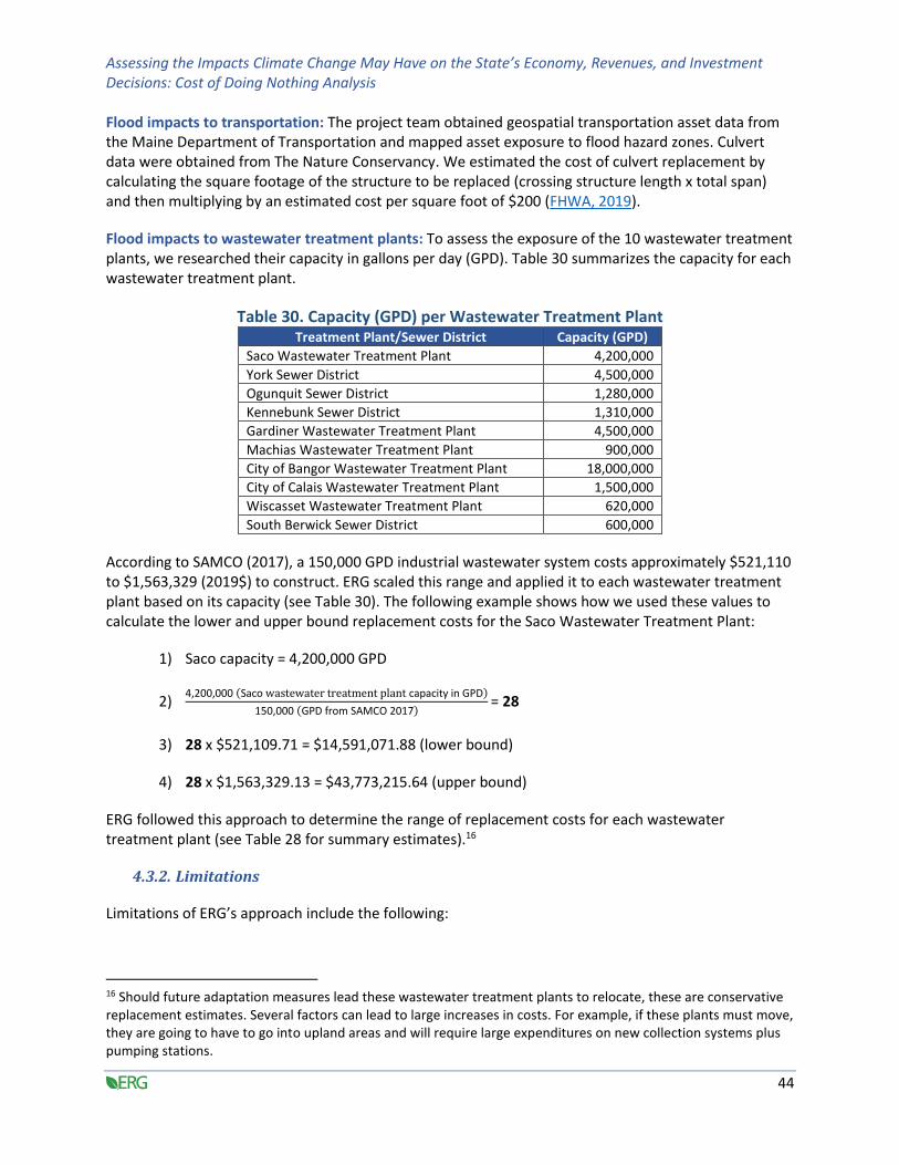
Assessing the Impacts Climate Change May Have on the State’s Economy, Revenues, and Investment Decisions: Cost of Doing Nothing Analysis
44
Flood impacts to transportation: The project team obtained geospatial transportation asset data from the Maine Department of Transportation and mapped asset exposure to flood hazard zones. Culvert data were obtained from The Nature Conservancy. We estimated the cost of culvert replacement by calculating the square footage of the structure to be replaced (crossing structure length x total span) and then multiplying by an estimated cost per square foot of $200 (FHWA, 2019).
Flood impacts to wastewater treatment plants: To assess the exposure of the 10 wastewater treatment plants, we researched their capacity in gallons per day (GPD). Table 30 summarizes the capacity for each wastewater treatment plant.
Table 30. Capacity (GPD) per Wastewater Treatment Plant Treatment Plant/Sewer District Capacity (GPD)
Saco Wastewater Treatment Plant 4,200,000
York Sewer District 4,500,000
Ogunquit Sewer District 1,280,000
Kennebunk Sewer District 1,310,000
Gardiner Wastewater Treatment Plant 4,500,000
Machias Wastewater Treatment Plant 900,000
City of Bangor Wastewater Treatment Plant 18,000,000
City of Calais Wastewater Treatment Plant 1,500,000
Wiscasset Wastewater Treatment Plant 620,000
South Berwick Sewer District 600,000
According to SAMCO (2017), a 150,000 GPD industrial wastewater system costs approximately $521,110 to $1,563,329 (2019$) to construct. ERG scaled this range and applied it to each wastewater treatment plant based on its capacity (see Table 30). The following example shows how we used these values to calculate the lower and upper bound replacement costs for the Saco Wastewater Treatment Plant:
1) Saco capacity = 4,200,000 GPD
2) 4,200,000 (Saco wastewater treatment plant capacity in GPD)
150,000 (GPD from SAMCO 2017)= 28
3) 28 x $521,109.71 = $14,591,071.88 (lower bound)
4) 28 x $1,563,329.13 = $43,773,215.64 (upper bound)
ERG followed this approach to determine the range of replacement costs for each wastewater treatment plant (see Table 28 for summary estimates).16
4.3.2. Limitations
Limitations of ERG’s approach include the following:
16 Should future adaptation measures lead these wastewater treatment plants to relocate, these are conservative replacement estimates. Several factors can lead to large increases in costs. For example, if these plants must move, they are going to have to go into upland areas and will require large expenditures on new collection systems plus pumping stations.

Assessing the Impacts Climate Change May Have on the State’s Economy, Revenues, and Investment Decisions: Cost of Doing Nothing Analysis
45
• Flood hazard data: FEMA’s National Flood Hazard Layer does not cover the entire state and is overdue for updates in some parts of Maine.
• Flood impacts to buildings: While HAZUS is the best available program to reasonably measure damage at such a large geographic scale, the accuracy of local results can be dependent on how well the tools building and infrastructure match reality. The lack of precision in the digital elevation model can also contribute to error in measurement. Additionally, the Hazus data are likely an underestimate of sea level rise damages, as they do not assume that buildings are a total loss. The model applies the depth-damage curve to assume lower damages at low flood levels. However, when a site is permanently inundated, the building is likely a loss regardless of the depth of flooding. When Hazus calculates damages under a 1 percent annual chance coastal event, it does not account for the effects of wind-driven waves, which can be damaging.
• Storm simulation model: This model has several limitations. We used a linear regression to derive the damages based on water level height, though this is likely not a linear relationship. This model is limited to exactly one storm event each year, when in reality, there may be several storms or no storms at all (the latter being unlikely). .
• Flood impacts to wastewater treatment plants: The cost to construct an industrial wastewater treatment system might differ from the cost of a municipal system. In addition, our method does not control for special considerations, such as the type of wastewater system implemented (e.g., zero liquid discharge systems versus more standard systems), which can vary in price compared to standard systems. The analysis does not quantify the vulnerability of the 10 wastewater treatment plants to one-time floods, as the values in Table 28 are only exposure estimates for inundation flooding from sea level rise.
• Flood impacts to transportation: Costs of culvert failures and crossings that restrict tidal flow (due to sea level rise) have not been evaluated.
4.3.3. Assumptions
Our approach assumes the following:
• Flood impacts to business: There were some limits to the calculations of GDP per job for each industry and each county. Employee GDP data were not available for every facility. In these cases, county GDP averages were applied; if necessary, a statewide average was applied.
• Flood impacts to transportation: We applied a $200 per square foot average cost for all culverts due to the ease of applying this value to the culvert data. The transportation analysis does not consider how flooded transportation assets could cut or limit access to major tourism sites, places of business, or other key community assets.
• Storm simulation model: This model has several assumptions. This model assumed that storm events would not increase in intensity or frequency by 2050. It also assumed that the baseline 1-year storm would occur every single year. This model assumed a linear relationship between damage and sea level rise and that sea level rise and storm surge would cause the same amount of damage, though in reality sea level rise would likely be lasting and storm surge damage would not.
• Long-term impacts to employment and GDP: Our job loss model had several large assumptions. The first was that jobs were lost for exactly one year if their business was flooded. While some jobs may come back after a flooding event, this is likely to impact different industries and

Assessing the Impacts Climate Change May Have on the State’s Economy, Revenues, and Investment Decisions: Cost of Doing Nothing Analysis
46
businesses in very different ways. Second, if sea levels rose above a business, that job was permanently lost. There are likely many jobs that would move the business to a more secure location.
• Flood impacts to wastewater treatment plants: This specific analysis assumed that:
- Each wastewater treatment plant is a “standard system” and would thus cost $521,110 to $1,563,329 (2019$) to construct per 150,000 GPD capacity (SAMCO, 2017).
- The cost of industrial wastewater treatment systems does not differ from the cost of municipal wastewater systems.
- The capacity (GPD) listed on each wastewater treatment plant website was both current and accurate.
- One-time or 1 percent annual chance flood waters recede and only cause partial damages to, not complete loss of, wastewater treatment plants.
- One-time or 1 percent annual chance flood events can happen multiple times, even in the same year.
- Inundation flooding from sea level rise does not recede and results in complete loss of the affected wastewater treatment plants.
4.4. RECOMMENDATIONS FOR FUTURE ANALYSIS
Recommended future analysis includes:
• Re-running all analyses with improved riverine floodplain maps and projections.
• Analyzing the impact of sea level rise on local government tax base.
• Conducting site-specific studies of impacts to key tourism/hospitality assets.
• Calculating costs of inaction on road, rail, and ferry terminals as additional cost data become available. Include a focus on highest value transportation assets in the state.
• Conducting transportation asset- and corridor-specific assessments to evaluate costs of service disruptions and delays (e.g., canceled ferries due to storm tides, blocked rail lines due to flooding).
• Obtaining exact, lifetime capital cost data for each priority wastewater treatment plant to refine the estimates in Table 28.
• Estimating the potential losses that the 10 wastewater treatment plants will incur from periodic nuisance flooding that causes damages and service disruptions but does not necessarily result in complete infrastructure loss requiring plants to move locations.

Assessing the Impacts Climate Change May Have on the State’s Economy, Revenues, and Investment Decisions: Cost of Doing Nothing Analysis
47
5. EROSION OF BEACHES AND DUNES
5.1. INTRODUCTION
Erosion of beaches can lead to the loss of tourism dollars and decreased beach experience, as well as the loss of ecosystem values. Based on 2018 statistics from the Maine Office of Tourism, the most popular region for leisure tourists and the most frequent primary destination for both day and overnight visitors is the Maine Beaches region of the southern Maine coastline (Maine Office of Tourism, 2018b). Beaches in this region also support over 28,000 jobs and bring in $164.9 million (2018$) in taxes (Maine Office of Tourism, 2018a). Moreover, beaches and dunes provide essential ecosystem services such as habitats that support coastal biodiversity as well as natural protection from flooding. However, as sea level rise due to climate change erodes beaches and damages beach-dune systems, some of the natural and recreational services beaches provide will disappear (Maine Climate Council Scientific and Technical Subcommittee, 2020). This will result in tangible losses to Maine’s coastal economy.
5.2. RESULTS
Out of the approximately 45 million day and overnight visitors to Maine in 2018, an estimated 10.4 million17 went to the beach based on Maine visitor survey responses (Maine Office of Tourism, 2018b). More specifically, an estimated 13.6 million people visited the Maine Beaches region as a whole, which includes Old Orchard Beach (Maine Office of Tourism, 2018a). These visitors spent $1.7 billion in 2018, which corresponds to an average spending of $125 per visitor. However, if the sea level rises 1.6 feet, 3.9 feet, and 8.8 feet in the future, the dry beach area in this region will decrease by 43 percent, 74 percent, and 98 percent, respectively.
This loss in beach area will result in less beach visitation and tourism-related spending in the region. In the year 2050, for example, a 1.6 feet sea level rise scenario would result in 1.1 million fewer visitors in this region and a $136 million (2018$) loss in tourism spending annually.
These values only show the decrease in direct economic impact to the region based on visitor spending, but the total indirect economic losses would be greater. They also underestimate the losses to beach economies for the entire state; the Maine Beaches region made up approximately 30 percent of all Maine visitors in 2018 (Maine Office of Tourism, 2018a). Total tourism spending in the region is not exclusive to beaches, but losses in this region may better encapsulate losses to other industries (restaurants, hotels, etc.) that rely on beach visitors.
17 Based on percentage of overnight and day visitors who indicated they were interested in water activities during their trip to Maine, and of those, the percentage of overnight and day visitors who indicated they went to the beach during their trip. We derived these values from surveys of overnight and day visitors to Maine carried out by DPA in collaboration with the Maine Office of Tourism (Maine Office of Tourism, 2018b).
Applicable Working Group(s):
Building, Infrastructure,
Housing Coastal and Marine Energy Natural Working Lands Resilience Transportation

Assessing the Impacts Climate Change May Have on the State’s Economy, Revenues, and Investment Decisions: Cost of Doing Nothing Analysis
48
These results also do not account for loss of beachgoer welfare. However, with 1.6 feet of sea level rise and an average 43 percent dry beach loss across Maine’s coast, ERG calculated an up to $39 million decrease in consumer surplus associated with beach trips, which better reflects the likely loss in beach experience that would result from less dry beach. Table 31 summarizes these results.
Table 31. Beach and Tourism Economic Loss for Sea Level Rise Scenarios Sea Level Rise
Scenario Percent Total Dry
Beach Loss Percent Lost Attendance
Number of Tourists Lost
Annual Spending Loss
(2018$)
1.6 ft 42% 8% 1,088,000 $136,000,000
3.9 ft 75% 45% 6,120,000 $765,000,000
8.8 ft 98% 98% 13,328,000 $1,666,000,000
Beyond tourism, Maine beaches and dunes offer a variety of ecosystem services such as (Troy, 2012):
• Water filtration
• Carbon cycling
• Flood protection
• Species habitats
• Disturbance regulation
Sand dunes are essential to biodiversity and resilience in Maine’s coastal communities, but between 85 percent and 100 percent of dunes in all counties will be inundated at 8.8 feet of sea level rise. The Maine beach-dune system’s ecosystem services have been valued at an average of approximately $104,715 (2018$ adapted from 2011$) or a total of approximately $71,836,000 (2018$ adapted from 2011$) (Troy, 2012).
Between waning beach areas and disappearing dunes, the overall value of beach ecosystem services, along with beach tourism, will decrease significantly if Maine communities do not take any further mitigating actions in the face of climate change.
5.3. METHODS
5.3.1. Data
5.3.1.1. Dry Beach and Tourism Loss
The Maine Office of Tourism estimates the number of visitors and tourism-related trips in Maine by region,18 including the Maine Beaches, Downeast and Acadia, Maine Highlands, Maine Lakes and Mountains, Mid-Coast, Greater Portland and Casco Bay, Kennebec Valley, and Aroostook County regions. Although the Maine Beaches region does not account for all state beaches, it is the most popular tourist region, and York County has the largest area of dry beaches of any coastal county (Maine Office of Tourism, 2018b; Dickson, Slovinsky, & Kelley, in preparation). In addition, most of this region’s tourist attractions center around coastal property, water activities, and beachgoing. Therefore, this
18 Estimates based on the National Omnibus Survey and modeled by DPA in collaboration with the Maine Office of Tourism (Maine Office of Tourism, 2018b).

Assessing the Impacts Climate Change May Have on the State’s Economy, Revenues, and Investment Decisions: Cost of Doing Nothing Analysis
49
region’s economy is tied to beach and ocean vitality. The Maine Beaches is approximately the same region as York County, pictured in Figure 8 below. We will use York County beach area data for the analysis in Table 32.
Figure 8. The Maine Beaches Region
Source: Maine Tourism Association
The estimated 13.6 million total visitors on tourism-related trips to these beaches spent $1.70 billion in 2018 in the categories shown in Figure 9. This value accounts for all tourism spending in the region, which is largely centered around beaches, and corresponds to an average spending of $125 per visitor.

Assessing the Impacts Climate Change May Have on the State’s Economy, Revenues, and Investment Decisions: Cost of Doing Nothing Analysis
50
Figure 9. Breakdown of Maine Beaches Visitor Spending in 2018
Source: Maine Office of Tourism (2018a) Regional Tourism Impact Estimates
The Maine Climate Council’s Science and Technology Subcommittee estimated the loss of dry beach and dunes for three sea level rise scenarios:
• HAT + 1.6 feet sea level rise
• HAT + 3.9 feet sea level rise
• HAT + 8.8 feet sea level rise
Table 32 shows the expected loss in acres, as well as percentage loss, of dry beaches for six of the eight coastal counties in Maine. It also shows the total losses for the six counties on the coastline for the three sea level rise scenarios (Dickson, Slovinsky, & Kelley, in preparation). As the Maine Beaches region is in York County, we will use the dry beach loss percentages for York County going forward.
Table 32. Dry Beach Loss for Sea Level Rise Scenarios
County [a]
Existing Dry
Beach (Acres)
[b]
HAT + 1.6 ft Sea Level Rise Scenario
HAT + 3.9 ft Sea Level Rise Scenario
HAT + 8.8 ft Sea Level Rise Scenario
Remaining (Acres)
Lost (Acres)
% Lost Remaining
(Acres) Lost
(Acres) % Lost
Remaining (Acres)
Lost (Acres)
% Lost
York 143.3 82.4 60.9 42% 36.4 106.9 75% 2.3 141.0 98%
Cumberland 48.0 27.1 21.2 44% 12.5 35.7 74% 1.4 46.8 97%
Sagadahoc 63.4 38.4 25.0 39% 19.5 43.9 69% 5.3 58.1 92%
Lincoln 2.0 0.7 1.3 65% 0.1 1.9 95% 0.0 2.0 100%
Knox 8.8 2.5 6.3 72% 0.5 8.3 94% 0.0 8.8 100%
Waldo 1.9 0.9 1.0 53% 0.2 1.8 90% 0.0 1.9 100%
Total 267.4 152.0 115.7 43% 69.2 198.4 74% 9.0 258.6 97% [a] Dry beach area mapping not completed yet for Hancock or Washington Counties.
[b] Dry beach is the approximate area between the seaward edge of dune or wall and the HAT.
Figures may not add to totals due to rounding.
Source: Dickson, Slovinsky, & Kelley, in preparation
Retail Sales28%
Restaurant Food29%
Lodging25%
Gasoline7%
Recreation10%
Other Transportation1%
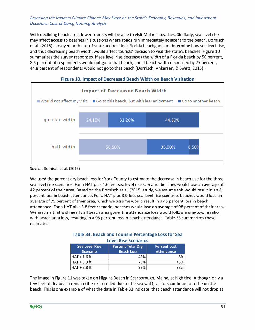
Assessing the Impacts Climate Change May Have on the State’s Economy, Revenues, and Investment Decisions: Cost of Doing Nothing Analysis
51
With declining beach area, fewer tourists will be able to visit Maine’s beaches. Similarly, sea level rise may affect access to beaches in situations where roads run immediately adjacent to the beach. Dornisch et al. (2015) surveyed both out-of-state and resident Florida beachgoers to determine how sea level rise, and thus decreasing beach width, would affect tourists’ decision to visit the state’s beaches. Figure 10 summarizes the survey responses. If sea level rise decreases the width of a Florida beach by 50 percent, 8.5 percent of respondents would not go to that beach, and if beach width decreased by 75 percent, 44.8 percent of respondents would not go to that beach (Dornisch, Ankersen, & Swett, 2015).
Figure 10. Impact of Decreased Beach Width on Beach Visitation
Source: Dornisch et al. (2015)
We used the percent dry beach loss for York County to estimate the decrease in beach use for the three sea level rise scenarios. For a HAT plus 1.6 feet sea level rise scenario, beaches would lose an average of 42 percent of their area. Based on the Dornisch et al. (2015) study, we assume this would result in an 8 percent loss in beach attendance. For a HAT plus 3.9 feet sea level rise scenario, beaches would lose an average of 75 percent of their area, which we assume would result in a 45 percent loss in beach attendance. For a HAT plus 8.8 feet scenario, beaches would lose an average of 98 percent of their area. We assume that with nearly all beach area gone, the attendance loss would follow a one-to-one ratio with beach area loss, resulting in a 98 percent loss in beach attendance. Table 33 summarizes these estimates.
Table 33. Beach and Tourism Percentage Loss for Sea Level Rise Scenarios
Sea Level Rise Scenario
Percent Total Dry Beach Loss
Percent Lost Attendance
HAT + 1.6 ft 42% 8%
HAT + 3.9 ft 75% 45%
HAT + 8.8 ft 98% 98%
The image in Figure 11 was taken on Higgins Beach in Scarborough, Maine, at high tide. Although only a few feet of dry beach remain (the rest eroded due to the sea wall), visitors continue to settle on the beach. This is one example of what the data in Table 33 indicate: that beach attendance will not drop at

Assessing the Impacts Climate Change May Have on the State’s Economy, Revenues, and Investment Decisions: Cost of Doing Nothing Analysis
52
the same rate as eroded dry beach, and that some visitors will still visit beaches that have significantly eroded.
Figure 11. Visitors at an Eroded Beach
Photo courtesy of Charlie Colgan (2018)
We assume that as beach area decreases, the number of visitors will decrease, but each visitor will spend the same amount of time there. Therefore, to estimate the visitor and economic losses to the Maine Beaches region, we applied the percent attendance lost in Table 33 to the 13.6 million visitors and the $1.70 billion they spent in 2018. This likely overestimates the losses, as it does not account for spending by tourists in the region who do not go to the beach at all.
5.3.1.2. Dry Beach and Consumer Surplus Loss
In 2016, Bell et al. surveyed beachgoers at Popham Beach State Park in Maine on their perceptions of changing shorelines (e.g., decreasing beach width from erosion), the effect of those changing shorelines on their experience, and their opinions about management and education surrounding this phenomenon (Bell, Noblet, & Scott, 2016). Like the Dornisch et al. (2015) study, this survey asked whether a one-half decrease in beach width would make their experience better, worse, or have no effect. To this, 0.5 percent of survey respondents answered the one-half width reduction would improve their experience, 46.3 percent answered it would worsen, and 53.2 percent answered it would have no effect (Bell & Noblet, 2017). Participants then answered whether the increased or decreased experience would cause them to take more or fewer trips to the beach. Based on the surveyed sample, the mean number of beach trips in the survey year (revealed preference) was 3.96, and the mean number of hypothetical beach trips with the erosion scenario (stated preference) was 3.75 (Bell & Noblet, 2017).
Using this revealed and stated preference data along with estimated travel cost to the beach, Bell and Noblet (2017) calculated that the mean change in consumer surplus per trip to Popham Beach State Park would be -$11.48 (2018$ adapted from 2017$) as a result of a one-half beach width reduction. We estimated the number of visitors to Maine beaches throughout the state using data from the Maine Office of Tourism. We multiplied the total number of visitors by the percent of visitors who said they

Assessing the Impacts Climate Change May Have on the State’s Economy, Revenues, and Investment Decisions: Cost of Doing Nothing Analysis
53
were interested in participating in water activities and, of those, the percent of visitors who said they went to the beach during their visit (Maine Office of Tourism, 2018b). We then divided the number of beach visitors (10.4 million) by 3, which was the average number of visitors per party, to approximate the number of beach trips with the number of parties that visited a Maine beach. Next, we multiplied the number of beach trips by the loss in consumer surplus per trip to calculate a $39.8 million loss in consumer surplus throughout Maine. This calculation takes 10.4 million visitors in the survey year and accounts for decreased beach visitation as a result of a one-half beach width reduction.
This loss in consumer surplus from a 50 percent decrease in beach width approximately aligns with the beach erosion expected across Maine in our HAT plus 1.6 feet sea level rise scenario.
5.3.1.3. Dune and Ecosystem Services Loss
We used the same three sea level rise scenarios to model dune loss for both developed and undeveloped dunes in Table 34 (Dickson, Slovinsky, & Kelley, in preparation). D1, or frontal dunes, are more dynamic and at risk during times of flooding and erosion than D2, or back dunes.
Table 34. Developed and Undeveloped Dune Loss
County
% Undeveloped Dunes Inundated % Developed Dunes Inundated
D1 (Frontal Dunes) D2 (Back Dunes)
All D1 (Frontal
Dunes) D2 (Back Dunes)
All
Dunes Inundated by HAT + 1.6 ft Sea Level Rise Scenario
York 10% 40% 29% 59% 94% 84%
Cumberland 59% 25% 39% 52% 94% 89%
Sagadahoc 62% 82% 74% 27% 83% 77%
Lincoln 76% 64% 69% 100% 58% 89%
Knox 91% 81% 88% 98% 100% 98%
Waldo 99% 72% 84% 97% 98% 98%
Hancock 92% 90% 91% 90% 82% 88%
Washington 91% 87% 90% 85% 77% 75%
Dunes Inundated by HAT + 3.9 ft Sea Level Rise Scenario
York 79% 94% 88% 90% 98% 96%
Cumberland 90% 85% 87% 75% 98% 96%
Sagadahoc 90% 93% 92% 52% 94% 89%
Lincoln 95% 97% 97% 100% 100% 100%
Knox 99% 99% 99% 100% 100% 100%
Waldo 100% 97% 98% 100% 100% 100%
Hancock 98% 99% 99% 99% 99% 99%
Washington 98% 99% 99% 81% 89% 85%
Dunes Inundated by HAT + 8.8 ft Sea Level Rise Scenario
York 85% 100% 94% 100% 100% 100%
Cumberland 100% 98% 99% 100% 100% 100%
Sagadahoc 99% 99% 99% 99% 99% 99%
Lincoln 100% 100% 100% 100% 96% 99%
Knox 100% 100% 100% 100% 100% 100%
Waldo 100% 100% 100% 100% 100% 100%
Hancock 100% 100% 100% 100% 100% 100%
Washington 100% 100% 100% 100% 100% 100% Source: Dickson, Slovinsky, & Kelley, in preparation
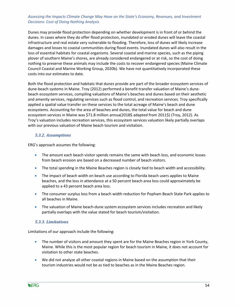
Assessing the Impacts Climate Change May Have on the State’s Economy, Revenues, and Investment Decisions: Cost of Doing Nothing Analysis
54
Dunes may provide flood protection depending on whether development is in front of or behind the dunes. In cases where they do offer flood protection, inundated or eroded dunes will leave the coastal infrastructure and real estate very vulnerable to flooding. Therefore, loss of dunes will likely increase damages and losses to coastal communities during flood events. Inundated dunes will also result in the loss of essential habitats for coastal organisms. Several coastal and marine species, such as the piping plover of southern Maine’s shores, are already considered endangered or at risk, so the cost of doing nothing to preserve these animals may include the costs to recover endangered species (Maine Climate Council Coastal and Marine Working Group, 2020b). We have not quantitatively incorporated these costs into our estimates to date.
Both the flood protection and habitats that dunes provide are part of the broader ecosystem services of dune-beach systems in Maine. Troy (2012) performed a benefit transfer valuation of Maine’s dune-beach ecosystem services, compiling valuations of Maine’s beaches and dunes based on their aesthetic and amenity services, regulating services such as flood control, and recreation services. Troy specifically applied a spatial value transfer on these services to the total acreage of Maine’s beach and dune ecosystems. Accounting for the area of beaches and dunes, the total value for beach and dune ecosystem services in Maine was $71.8 million annua(2018$ adapted from 2011$) (Troy, 2012). As Troy’s valuation includes recreation services, this ecosystem services valuation likely partially overlaps with our previous valuation of Maine beach tourism and visitation.
5.3.2. Assumptions
ERG’s approach assumes the following:
• The amount each beach visitor spends remains the same with beach loss, and economic losses from beach erosion are based on a decreased number of beach visitors.
• The total spending in the Maine Beaches region is closely tied to beach width and accessibility.
• The impact of beach width on beach use according to Florida beach users applies to Maine beaches, and the loss in attendance at a 50 percent beach area loss could approximately be applied to a 43 percent beach area loss.
• The consumer surplus loss from a beach width reduction for Popham Beach State Park applies to all beaches in Maine.
• The valuation of Maine beach-dune system ecosystem services includes recreation and likely partially overlaps with the value stated for beach tourism/visitation.
5.3.3. Limitations
Limitations of our approach include the following:
• The number of visitors and amount they spent are for the Maine Beaches region in York County, Maine. While this is the most popular region for beach tourism in Maine, it does not account for visitation to other state beaches.
• We did not analyze all other coastal regions in Maine based on the assumption that their tourism industries would not be as tied to beaches as in the Maine Beaches region.

Assessing the Impacts Climate Change May Have on the State’s Economy, Revenues, and Investment Decisions: Cost of Doing Nothing Analysis
55
• Impacts of dune inundation heavily depends on the location and surrounding infrastructure, so we did not generalize dune loss for the state.
• We modeled beach and dune loss on static inundation and did not account for erosion caused by higher sea levels.
5.4. RECOMMENDATIONS FOR FUTURE ANALYSIS
Recommendations for future analysis of beach erosion on tourism and ecosystem services include:
• Incorporating data for all Maine beaches with projected erosion rates.
• Accounting for potential decreased willingness to pay or spending as beach width decreases.
• Quantifying the effect of dune loss and beach area loss on loss of ecosystem services value, accounting for the unique values provided by different dune and beach sites.
• Evaluating the key issue of beach access, recognizing that in some cases beach access roads might be more vulnerable than the beaches themselves. As a starting point, consider beaches such as Gooch’s/Kennebunk Beach, Long Sands Beach in York, and the entire Saco Bay system, which each have roads immediately adjacent to the beach.

Assessing the Impacts Climate Change May Have on the State’s Economy, Revenues, and Investment Decisions: Cost of Doing Nothing Analysis
56
6. VECTOR-BORNE ILLNESS
6.1. INTRODUCTION
Tick-borne diseases, specifically Lyme disease, anaplasmosis, babesiosis, and Powassan encephalitis virus, have been growing in geographic extent and case numbers since the early 1980s and are a major public health concern in Maine. Increased incidences of Lyme disease, babesiosis, and anaplasmosis are associated with range expansion of the deer tick (Cavanaugh et al., 2017), while deer tick range expansion is attributed to expanding white-tailed deer populations, suburban development in forested areas, and warmer/shorter winters—with the change in winter season caused by climate change (Fernandez et al., 2020).
Escalating Lyme infection rates are particularly concerning, with disease symptoms that can include arthritis, Bell's palsy and other cranial nerve palsies, meningitis, and carditis. These symptoms lead to costly medical treatments, income loss, and lower quality of life. As such, we evaluated current costs of the disease and how they may change.
Mosquito-borne diseases, such as eastern equine encephalitis, are also a concern in Maine. Eastern equine encephalitis has no treatment and a high mortality rate. The disease circulates among tree hole mosquitos, birds, and mammals. Climate change leads to increases in summer precipitation and humidity, increased frequency of extreme rain events, earlier degree day accumulation, and warmer falls, which create conditions that exacerbate eastern equine encephalitis transmission (Birkel & Mayewski, 2018).
Two Maine residents have had confirmed eastern equine encephalitis to date (2014, 2015), with one case being fatal. It is important to understand the costs of eastern equine encephalitis because outbreaks are expected to increase.
6.2. RESULTS
Lyme disease: Current costs to treat Lyme disease patients in the state are approximately $11.5 million each year (for the 1,405 cases in 2018). Although various studies project expansion of deer tick range and abundance under future climate change and land use scenarios, it is not currently possible to use tick abundance to directly project case numbers (Sagurova et al., 2019). While expanding tick range and numbers are an indicator of more Lyme disease cases, a clear linear relationship has not been established between tick abundance and Lyme cases. As such, we can expect Lyme disease case numbers and costs will continue to increase beyond $11.5 million annually without tick control efforts and related actions. A multitude of factors impact rates of infection and symptomatic patients, making it challenging to project specific case numbers in the event of no action.
Eastern equine encephalitis: While it is also challenging to project future eastern equine encephalitis outbreaks in Maine, the science indicates that they are likely to rise (Birkel & Mayewski, 2018). There is a range of costs to consider for eastern equine encephalitis patients. A cost study based on a Massachusetts outbreak found that those who suffered a transient episode faced approximately
Applicable Working Group(s):
Building, Infrastructure,
Housing Coastal and Marine Energy Natural Working Lands Resilience Transportation

Assessing the Impacts Climate Change May Have on the State’s Economy, Revenues, and Investment Decisions: Cost of Doing Nothing Analysis
57
$40,360 (2018$) in direct medical costs. Direct costs of intervention for those who suffered from residual sequela as a result of eastern equine encephalitis were about $5.76 million (2018$) per patient during their life (Villari, 1995). Clearly, costs would quickly multiply in the case of a major outbreak.
6.3. METHODS
6.3.1. Data
Lyme disease: In 2018, the Maine CDC reported 1,405 Lyme disease cases in the state, a decline from the record high in 2017. While final totals have not been confirmed, Maine CDC said it received a record high number of reports from health providers in 2019, with 2,079 cases (as of January 17, 2020) (Peranzi & Robinson, 2020).
A 2006 study in Maryland estimates that a Lyme disease patient (whether early or late stage) incurs an annual average of $4,273 in direct medical costs plus $7,485 (2019$) in indirect medical costs, nonmedical costs, and productivity losses (Zhang et al., 2006). These direct medical costs are supported by a national-level study in 2015 that estimates Lyme disease is associated with $3,200 (2019$ adapted from 2015$) in higher total annual health care costs (Adrion et al., 2015). If we apply the costs from the Maryland study, we can assume that Lyme disease costs (whether incurred by the state or patient) are $4,273 for direct medical costs plus $7,485 for indirect costs for a total annual cost of almost $12,209 (2019$). Drawing on Maine’s 2018 infection numbers (1,405), the total cost associated with infections from that year is approximately $16.7 million.
Eastern equine encephalitis: We have used costs of an outbreak in Massachusetts as a reference for potential costs of an outbreak in Maine.
6.3.2. Assumptions
This cost estimate assumes similar costs between Lyme patients on the Maryland Eastern Shore and all of Maine. In addition, this approach assumes that costs have not changed significantly between 1997 and 2018 (1997 costs were converted to 2018 equivalent). A national-scale study (from 2015) confirmed similar costs.
This cost estimate also assumes similar costs between eastern equine encephalitis patients in eastern (in the Boston suburbs) and southern (near Fall River and New Bedford) Massachusetts and potential eastern equine encephalitis patients across Maine. In addition, it assumes that costs of treatment have not changed significantly since the outbreaks in the 1980s.
6.3.3. Limitations
This analysis of costs of Lyme disease is based on numbers that the Maine CDC collects each year on new infections. This number does not represent the number of people struggling with symptoms of the disease at any given time. As such, the costs presented are likely an underestimate.
6.4. RECOMMENDATIONS FOR FUTURE ANALYSIS
As reliable projections of future cases become available, they should be used to improve future cost estimates. Future analysis should include the cost of veterinary outbreaks and costs associated with

Assessing the Impacts Climate Change May Have on the State’s Economy, Revenues, and Investment Decisions: Cost of Doing Nothing Analysis
58
additional tick and mosquito-borne diseases that are expected to expand in range and impacts to Mainers in our changing climate.

Assessing the Impacts Climate Change May Have on the State’s Economy, Revenues, and Investment Decisions: Cost of Doing Nothing Analysis
59
7. FISHING AND AQUACULTURE INDUSTRIES
7.1. INTRODUCTION
The fishing and aquaculture sector is a vital part of the Maine economy and culture. As of 2020, marine aquaculture accounted for 622 jobs, an increase of about 9 percent since 2014 (Cole, Langston, & Davis, 2017). Employment in this industry, as shown in Figure 12, is largely concentrated along the shorelines of Maine. As a result, this sector can be sensitive to climate change impacts from ocean warming and ocean acidification. Within the fishing and aquaculture sector, the lobster industry provides the single greatest fisheries product for the state, accounting for over 73 percent of landings value for the year 2019 (Maine Department of Marine Resources, 2020).
Applicable Working Group(s):
Building, Infrastructure,
Housing Coastal and Marine Energy Natural Working Lands Resilience Transportation

Assessing the Impacts Climate Change May Have on the State’s Economy, Revenues, and Investment Decisions: Cost of Doing Nothing Analysis
60
Figure 12. Relative Employment by Census Tract, Fishing Industry

Assessing the Impacts Climate Change May Have on the State’s Economy, Revenues, and Investment Decisions: Cost of Doing Nothing Analysis
61
7.2. RESULTS
The lobster industry is very important to Maine’s economy, comprising a significant proportion of the state’s total commercial landings value. Maine’s lobster landings make up 80 percent of the entire U.S. lobster industry (Maine Climate Council Scientific and Technical Subcommittee, 2020). Based on preliminary data for 2019, no other species makes up even 5 percent of the over $670 million in annual commercial landings value for Maine (Maine Department of Marine Resources, 2020). The total value of lobster landings for 2019 is estimated at about $485 million (2019$), or 73 percent of all commercial landings in Maine, as shown in Figure 13 (Maine Department of Marine Resources, 2020). Lobster landings are split by county in Table 35, which shows that Cumberland and York Counties account for about $75 million in value (Maine Department of Marine Resources, 2020). These two counties, the southernmost in Maine, are most at risk to losses due to rising ocean temperatures.
Figure 13. Preliminary 2019 Commercial Landings by Ex-Vessel Value
Note: Other species include confidential species and species that make up less than 1 percent of total catch.
Table 35. Lobster Landings by County, 2019 County Weight (Millions of lbs.) Value (Millions of 2019$)
Cumberland 10.72 $55.05
Hancock 31.62 $152.30
Knox 27.15 $139.28
Lincoln 5.19 $26.32
Sagadahoc 1.18 $6.04
Waldo 0.63 $3.11
Washington 20.48 $83.76
York 3.75 $19.55
Total 100.73 $485.41
The overall value of Maine’s aquaculture harvests has increased over the last decade. In 2019, Maine experienced its highest total harvest value in the past decade at over $88 million (Maine Department of

Assessing the Impacts Climate Change May Have on the State’s Economy, Revenues, and Investment Decisions: Cost of Doing Nothing Analysis
62
Marine Resources, 2020). By 2050, estimates suggest that total harvest value in Maine could be nearly $168 million. In terms of employment, the aquaculture industry had 571 workers as of 2014 (Cole, Langston, & Davis, 2017). The number of jobs in this industry is now estimated to be 622 in 2020. Aquaculture employment is expected to increase to about 1,300 by the year 2050. Both 2050 projections, however, do not consider the risks of climate change and their impact on aquaculture. This potential for growth is at risk if mitigative efforts are not taken soon.
As explained in the Introduction to this report, we can artificially decrease economic output (i.e., revenue) in an industry to explore how the state economy would react to the shocks from climate change in specific industries (in this case fishing). If we consider a linear decline to 50% by 2050 in the revenue of the fishing industry, Maine’s economy would see a 0.7% revenue reduction by 2050. So, while a 50% reduction would drastically impact the fishing industry, it would also have larger impacts on the entire state economy.
Spikes in sea surface temperature in the recent past have corresponded with earlier season peaks for lobster harvesting specifically. Table 36 provides sea surface temperature data from the University of Maine showing that temperatures spiked in 2012 and 2016. The largest year-to-year increase in total weight of lobster landings occurred in 2012, while the greatest total weight and value of lobster landings was in 2016, according to historical Maine fisheries landings data from Maine’s Department of Marine Resources (Maine Department of Marine Resources, 2020). Other factors besides warming waters can affect these year-to-year differences. Warmer weather can encourage longer fishing seasons and even longer days as lobstermen take advantage of the conditions. Lobstermen may also try to compensate for low prices due to an abundance of lobsters by making a greater effort to catch more lobsters.
Table 36. Sea Surface Temperature Anomalies and Lobster Landings, 2004–2019
Year Gulf of Maine Avg Sea Surface
Temperature Anomaly (°F) Weight (Millions of lbs.) Value (Millions of 2019$)
2004 0.40 71.5742 289.0788
2005 2.22 68.7299 317.9483
2006 3.80 75.3458 305.4394
2007 1.93 63.976 280.6484
2008 2.18 69.9085 245.15
2009 2.29 81.1746 237.5369
2010 4.58 96.2088 318.0524
2011 3.68 104.9247 334.5397
2012 7.60 127.3214 342.0795
2013 5.06 127.8084 370.384
2014 5.22 124.3259 459.5084
2015 5.37 122.6634 502.4503
2016 7.40 132.4908 540.183
2017 5.58 111.9823 438.516
2018 4.56 121.3212 491.5869
2019 [a] 3.28 100.725 485.405
[a] 2019 lobster data are preliminary.
This is not to say that ocean warming will positively impact Maine’s lobster industry outlook. Some projections predict that lobster abundance will decline by about 45 percent by the year 2050 given increasingly warmer ocean temperatures (Le Bris et al., 2018). Increased temperatures could also lead to a northward shift of lobsters, hampering related fisheries activity in the Gulf of Maine. The migration of
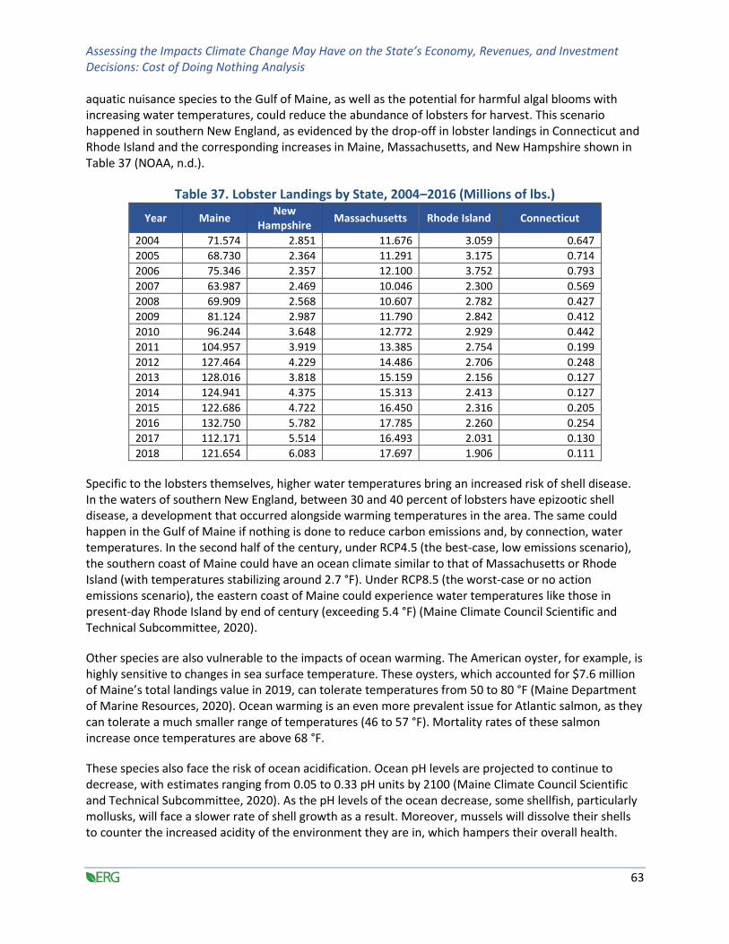
Assessing the Impacts Climate Change May Have on the State’s Economy, Revenues, and Investment Decisions: Cost of Doing Nothing Analysis
63
aquatic nuisance species to the Gulf of Maine, as well as the potential for harmful algal blooms with increasing water temperatures, could reduce the abundance of lobsters for harvest. This scenario happened in southern New England, as evidenced by the drop-off in lobster landings in Connecticut and Rhode Island and the corresponding increases in Maine, Massachusetts, and New Hampshire shown in Table 37 (NOAA, n.d.).
Table 37. Lobster Landings by State, 2004–2016 (Millions of lbs.)
Year Maine New
Hampshire Massachusetts Rhode Island Connecticut
2004 71.574 2.851 11.676 3.059 0.647
2005 68.730 2.364 11.291 3.175 0.714
2006 75.346 2.357 12.100 3.752 0.793
2007 63.987 2.469 10.046 2.300 0.569
2008 69.909 2.568 10.607 2.782 0.427
2009 81.124 2.987 11.790 2.842 0.412
2010 96.244 3.648 12.772 2.929 0.442
2011 104.957 3.919 13.385 2.754 0.199
2012 127.464 4.229 14.486 2.706 0.248
2013 128.016 3.818 15.159 2.156 0.127
2014 124.941 4.375 15.313 2.413 0.127
2015 122.686 4.722 16.450 2.316 0.205
2016 132.750 5.782 17.785 2.260 0.254
2017 112.171 5.514 16.493 2.031 0.130
2018 121.654 6.083 17.697 1.906 0.111
Specific to the lobsters themselves, higher water temperatures bring an increased risk of shell disease. In the waters of southern New England, between 30 and 40 percent of lobsters have epizootic shell disease, a development that occurred alongside warming temperatures in the area. The same could happen in the Gulf of Maine if nothing is done to reduce carbon emissions and, by connection, water temperatures. In the second half of the century, under RCP4.5 (the best-case, low emissions scenario), the southern coast of Maine could have an ocean climate similar to that of Massachusetts or Rhode Island (with temperatures stabilizing around 2.7 °F). Under RCP8.5 (the worst-case or no action emissions scenario), the eastern coast of Maine could experience water temperatures like those in present-day Rhode Island by end of century (exceeding 5.4 °F) (Maine Climate Council Scientific and Technical Subcommittee, 2020).
Other species are also vulnerable to the impacts of ocean warming. The American oyster, for example, is highly sensitive to changes in sea surface temperature. These oysters, which accounted for $7.6 million of Maine’s total landings value in 2019, can tolerate temperatures from 50 to 80 °F (Maine Department of Marine Resources, 2020). Ocean warming is an even more prevalent issue for Atlantic salmon, as they can tolerate a much smaller range of temperatures (46 to 57 °F). Mortality rates of these salmon increase once temperatures are above 68 °F.
These species also face the risk of ocean acidification. Ocean pH levels are projected to continue to decrease, with estimates ranging from 0.05 to 0.33 pH units by 2100 (Maine Climate Council Scientific and Technical Subcommittee, 2020). As the pH levels of the ocean decrease, some shellfish, particularly mollusks, will face a slower rate of shell growth as a result. Moreover, mussels will dissolve their shells to counter the increased acidity of the environment they are in, which hampers their overall health.
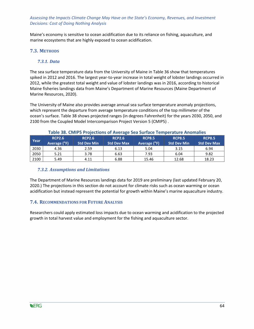
Assessing the Impacts Climate Change May Have on the State’s Economy, Revenues, and Investment Decisions: Cost of Doing Nothing Analysis
64
Maine’s economy is sensitive to ocean acidification due to its reliance on fishing, aquaculture, and marine ecosystems that are highly exposed to ocean acidification.
7.3. METHODS
7.3.1. Data
The sea surface temperature data from the University of Maine in Table 36 show that temperatures spiked in 2012 and 2016. The largest year-to-year increase in total weight of lobster landings occurred in 2012, while the greatest total weight and value of lobster landings was in 2016, according to historical Maine fisheries landings data from Maine’s Department of Marine Resources (Maine Department of Marine Resources, 2020).
The University of Maine also provides average annual sea surface temperature anomaly projections, which represent the departure from average temperature conditions of the top millimeter of the ocean’s surface. Table 38 shows projected ranges (in degrees Fahrenheit) for the years 2030, 2050, and 2100 from the Coupled Model Intercomparison Project Version 5 (CMIP5) .
Table 38. CMIP5 Projections of Average Sea Surface Temperature Anomalies
Year RCP2.6
Average (°F) RCP2.6
Std Dev Min RCP2.6
Std Dev Max RCP8.5
Average (°F) RCP8.5
Std Dev Min RCP8.5
Std Dev Max
2030 4.36 2.59 6.13 5.04 3.15 6.94
2050 5.21 3.78 6.63 7.93 6.04 9.82
2100 5.49 4.11 6.88 15.46 12.68 18.23
7.3.2. Assumptions and Limitations
The Department of Marine Resources landings data for 2019 are preliminary (last updated February 20, 2020.) The projections in this section do not account for climate risks such as ocean warming or ocean acidification but instead represent the potential for growth within Maine’s marine aquaculture industry.
7.4. RECOMMENDATIONS FOR FUTURE ANALYSIS
Researchers could apply estimated loss impacts due to ocean warming and acidification to the projected growth in total harvest value and employment for the fishing and aquaculture sector.
Assessing the Impacts Climate Change May Have on the State’s Economy, Revenues, and Investment Decisions: Cost of Doing Nothing Analysis
65
8. HIGH HEAT DAYS AND HEAT ILLNESS
8.1. INTRODUCTION
Maine’s average air temperature and number of high heat index days is projected to increase over the coming decades. Under the “business as usual” RCP8.5 scenario, Maine’s average air temperature is expected to be 6 °F warmer in 2050 and over 12 °F warmer by 2100. Under a scenario of moderate greenhouse gas emissions reductions (RCP4.5), Maine is expected to warm by 5 °F in 2050 and 6.5 °F in 2100. In the improbable event of rapidly transforming our carbon-intensive economy (RCP2.6), temperatures will stabilize around 4 °F. These rising average temperatures will increase the number of high heat index days (which feel like 90 °F or hotter). As compared to the average of one high heat day Maine experienced each year from 1971 to 2000, under RCP8.5, Maine can expect 14 high heat index days annually by 2050 and 36 by 2100. Under RCP4.5, the state can expect nine high heat index days each year by 2050 and 13 by 2100 (Union of Concerned Scientists, 2019).
Exposure to extreme heat is linked with a range of negative health outcomes, including heatstroke and heat exhaustion; renal failure; dehydration; exacerbations of existing cardiovascular, respiratory, cerebrovascular, and diabetes-related conditions; effects on fetal health; preterm births; and mental health conditions. Mainers are particularly vulnerable to these high heat days because residents of cooler climates are less physiologically adapted to extreme heat and experience disproportionate health effects (Anderson and Bell, 2011). In addition, air conditioning is one of the best defenses against heat, but adoption of air conditioning is far lower in Maine than in the rest of the country (53 percent of Maine households as opposed to 90 percent of U.S. households) (Maine CDC, 2020; U.S. EIA, 2018). Figure 14 maps communities across the state that are vulnerable to heat because they:
• Are over 65 years old and living alone
• Are under 5 years old
• Lack air conditioning
• Have a low population density
• Live in the warmer coastal and central climate divisions
Although we did not calculate the costs of heat illness specifically in these communities, it is important to be aware of the spatial distribution of vulnerability in preparing for high heat events.
Applicable Working Group(s):
Building, Infrastructure,
Housing Coastal and Marine Energy Natural Working Lands Resilience Transportation

Assessing the Impacts Climate Change May Have on the State’s Economy, Revenues, and Investment Decisions: Cost of Doing Nothing Analysis
66
Figure 14. Populations Vulnerable to High Heat
Note: Darker red communities exhibit all vulnerability characteristics.
8.2. RESULTS
Health care costs for heat illness are at least $224,000 today. With high heat days on the rise, this number could multiple many times. If emergency room visits and hospital visits are directly proportional to the number of days with a heat index over 90 °F, health care costs will be nine to 14 times higher in 2050 (costing $1.9-to $3.2 million annually) and 13 to 36 times higher (costing $2.9 to $8.1 million annually) in 2100. These direct health care costs do not account for lost wages, childcare, or indirect costs of heat illness. They also do not account for the disproportionate burden these costs and health impacts are expected to have on low-income and socially vulnerable communities (e.g., elderly, rural).

Assessing the Impacts Climate Change May Have on the State’s Economy, Revenues, and Investment Decisions: Cost of Doing Nothing Analysis
67
8.3. METHODS
8.3.1. Data
The Maine CDC (2020) reports that between May and September each year, Mainers experience an average of just over 200 emergency department visits and almost 15 hospitalizations for heat-related illnesses.
A study by the Healthcare Cost and Utilization Project (Merrill, Miller, & Steiner, 2008), based on a 2005 national sample, found that the average cost per heat-related hospital stay was $7,968 (2019$). The study also found that heat-related hospitalization rates increase as income levels decrease and are higher in rural areas. Applying this cost to the approximately 15 annual hospitalizations in Maine (under today’s conditions), we estimate that heat-related hospitalizations currently cost about $119,520.
The Health Care Cost Institute compiled a national data set of emergency department visits (broken down by state) from 2009 to 2015 to track changing and generally increasing costs of emergency department visits (Hargraces & Kennedy, 2017). The procedure codes tracked are key components of an emergency room visit and basic evaluation (as opposed to specific injections and treatments that a patient may subsequently receive). For Maine, these costs increase each year, with the average price per claim reaching $488 by 2015 ($524 in 2019$). If we assume that emergency room visits for approximately 200 heat illness patients today costs at least $524 per visit, the annual cost of these emergency room visits amounts to $104,800 today.
Health care costs for heat illness are at least $224,00 today. With high heat days on the rise, this number could multiple many times. If emergency room visits and hospital visits are directly proportional to the number of days with a heat index over 90 °F, health care costs will be nine to 14 times higher in 2050 (costing $1.9 to $3.2 million) and 13 to 36 times higher (costing $2.9 to $8.1 million) in 2100.
8.3.2. Assumptions
This approach to costing impacts of extreme heat on health assumes that impacts will be proportional to the number of high heat index days (over 90 °F), rather than proportional to the duration of high heat events or number of degrees above the 90 °F threshold.
8.3.2.1. Limitations
Estimates of emergency room costs have limitations. The Healthcare Cost Institute collected data on patients charged for emergency room procedure codes (CPT codes 99281–99285) (Hargraces & Kennedy, 2017). These costs represent the facility fee for an emergency room visit (i.e., the cost of receiving care in an emergency room instead of a doctor's office). They do not include the costs of other services patients received during their visit, such as an injected drug, and they are specific to treatments for a heat illness.
8.4. RECOMMENDATIONS FOR FUTURE ANALYSIS
Recommendations for future analysis of high heat include:
• Assessing broader economic implications, for example, in industries that require outdoor labor (i.e., how often work will need to cease or shift hours due to high heat).

Assessing the Impacts Climate Change May Have on the State’s Economy, Revenues, and Investment Decisions: Cost of Doing Nothing Analysis
68
• Conducting a detailed study of costs associated with emergency room visits specifically for heat illness.

Assessing the Impacts Climate Change May Have on the State’s Economy, Revenues, and Investment Decisions: Cost of Doing Nothing Analysis
69
9. CONCLUSION
This estimate of losses that the State of Maine and its citizens could incur if the State does not adapt to climate change makes it clear that that losses could be very large. This analysis of the cost of doing nothing focuses on key issues identified through a vulnerability mapping and assessment exercise and homes in on costs related to working group strategies. Therefore, this report does not cover all costs that could be incurred by the State and its citizens without climate adaptation and action. Costs may be even higher. As the report establishes our economic baseline, it helps to define the benefits of adaptation and mitigation actions. As such, the report provides key inputs into Volume 4: Economic Analysis of Adaptation and Mitigation Strategies which evaluates cost-benefit and cost-effectiveness of various strategies, to help inform strategy recommendations from the Maine Climate Council Working Groups.
FFDFD

Assessing the Impacts Climate Change May Have on the State’s Economy, Revenues, and Investment Decisions: Cost of Doing Nothing Analysis
70
REFERENCES Adler, M., Anthoff, D., Bosetti, V., Garner, G., Keller, K., and Treich, N. (2017). Priority for the worse-off
and the social cost of carbon. Nature Climate Change.
Adrion, E., Aucott, J., Lemke , K., & Weiner, J. (2015). Health Care Costs, Utilization and Patterns of Care following Lyme Disease. PLoS One, 1–14.
Arnell, N., & Gosling, S. (2016 ). The impacts of climate change on river flood risk at the global scale. Climate Change, 132 (3), 387-401.
ASMFC. (2017). 2017 Review of the Atlantic States Marine Fisheries Commission Fishery Management Plan for American Lobster. ASMFC.
Avallon, E. (2019). Presentation on Carbon Pricing and Market Design. NY ISO. Rensselaer, NY: https://www.nyiso.com/documents/20142/7129597/6.20.2019_MIWG_Carbon_Pricing_MDC_FINAL.pdf/cf67ebb8-d0fc-7b4b-100f-c3756d6afae8.
Bai, X., Daigneault, A., Fernandez, I., Frank, J., Hayes, D., Johnson, B., . . . Weiskittel, A. (2020). State of Maine's Carbon Budget, 2006-2016. Orno, ME: The University of Maine. Retrieved July 29, 2020, from https://crsf.umaine.edu/forest-climate-change-initiative/carbon-budget/
Bartow-Gillies, M. E. (2020). The Maine Tidal Restriction Database: A desktop assessment of tidal restrictions in Maine to facilitate community resilience and habitat restoration. Maine Coastal Program.
Bell, K. P., & Noblet, C. (2017). Environmental change and recreation demand. Seminar, Department of Economics, University of New Hampshire. School of Economics, University of Maine.
Bell, K. P., Noblet, C. L., & Scott, S. (2016). 2016 Popham Beach State Park. University of Maine School of Economics.
Birkel, S. D., & Mayewski, P. A. (2018). Coastal Maine Climate Futures. Orno, ME: Climate Change Institute, University of Maine.
Bureau of Economic Analysis. (2020, April 3). Table 1.1.9. Implicit price deflators for Gross Domestic Product. March 26, 2020. Retrieved from https://apps.bea.gov/iTable/iTable.cfm?reqid=19&step=2#reqid=19&step=2&isuri=1&1921=survey
Cai, Y., and Lontzek, T.S. (2019). The Social Cost of Carbon with Economic and Climate Risks. Journal of Political Economy, University of Chicago, 1-79.
California Air Resources Board. (2017). California's 2017 Climate Change Scoping Plan: the strategy for acheiving California's 2030 greenhouse gas target.
Cavanaugh, C., Muscat, P., Telford, S., Goethert, H., Pendlebury, W., Elias, S., . . . Smith, R. (2017). Fatal deer tick virus infection in Maine. Clinical Infectious Diseases, 1043-1046.
Cole, A., Langston, A., & Davis, C. (2017). Maine Aquaculture Economic Impact Report. University of Maine, Aquaculture Research Institute. Retrieved from https://cpb-us-w2.wpmucdn.com/wpsites.maine.edu/dist/1/43/files/2017/01/Aquaculture-Econ-Report-25i1qf3.pdf

Assessing the Impacts Climate Change May Have on the State’s Economy, Revenues, and Investment Decisions: Cost of Doing Nothing Analysis
71
Cole, S. G. (2016). Valuing multiple eelgrass ecosystem services in Sweden: fish production and uptake of carbon and nitrogen. Frontiers in Marine Science, 2, 121. doi:10.3389/fmars.2015.00121
Commission, M. P. (2015). Maine Distributed Solar Valuation Study. Clean Power Research.
Costanza, R. P.-M. (2008). The value of coastal wetlands for hurricane protection. AMBIO: A Journal of the Human Environment, 37(4), 241-248. doi:10.1579/0044-7447(2008)37[241:TVOCWF]2.0.CO;2
Daigneault, A., Simons-Legaard, E., Fernandez, I., Weiskittel, A., Birthisel, S., & Carroll, J. (2020). Maine Forestry and Agriculture Climate Change Mitigation Potential; Preliminary Results for Distribution and Review. Orno, ME: University of Maine.
Daymark Energy Advisors, R. E. (2018). Benefits and Costs of Utility-Scale and Behind-the-Meter Solar Resources in Maryland. Maryland Public Service Commission.
Demaria, E., Palmer, R., & Roundy, J. (2016a). Regional climate change projections of streamflow characteristics in the Northeast and Midwest US. Journal of Hydrology: Regional Studies, 309-323.
Dickson, S., Slovinsky, P., & Kelley, J. (in preparation). Sea Level Rise and Storm Surge. In Maine Climate Council Maine Science and Technology Subcommittee, Scientific Assessment of Climate Change and Its Effects in Maine.
Dornisch, V. D., Ankersen, T. T., & Swett, R. A. (2015). Florida beach users’ perceptions of beach ownership, erosion management, and sea level rise. University of Florida Conservation Clinic, University of Florida Levin College of Law.
Drake, K. H. (2015). Carbon sequestration in tidal salt marshes of the Northeast United States. Environmental management, 56(4), 998-1008. doi:10.1007/s00267-015-0568-z
Eastern Reserach Group, I. (2020). Assessing the Impacts Climate Change May Have on the State's Economu, Revenues, and Investments: Volume 1. Vulnerability Mapping.
Ebi, K., Balbus, J., Luber , G., Bole, A., Crimmins, A., Glass, G., . . . White-Newsome, J. (2018). 2018: Human Health. In Impacts, Risks, and Adaptation in the United States: Fourth National Climate Assessment, Volume II. pp. 539–571. (D. C. Reidmiller, Ed.) Washington, DC, USA: U.S. Global Change Research Program. doi:10.7930/NCA4.2018.CH14
Ekstrom, J. A., Suatoni, L., Cooley, S. R., Pendleton, L. H., Waldbusser, G. G., Cinner, J. E., . . . Brander, L. M. (2015). Vulnerability and adaptation of US shellfisheries to ocean acidification. Nature Climate Change, 5(3), 207-214.
Environment, S. o. (2019). 2019 Greenhouse Gas Emissions Reduction Act Plan. State of Maryland Department of the Environment.
EPA. (2016, December). Fact Sheet: Social Cost of Carbon. Retrieved from https://www.epa.gov/sites/production/files/2016-12/documents/social_cost_of_carbon_fact_sheet.pdf
Executive Order 13783: Promoting Energy Independence and Economic Growth (Federal Register 2017).
Fernandez, I., Birkel, S., Schmitt, C., Simonson, J., Lyon, B., Pershing, A., . . . Mayewski, P. (2020). Maine's Climate Future: 2020 Update. Orono: University of Maine.
Assessing the Impacts Climate Change May Have on the State’s Economy, Revenues, and Investment Decisions: Cost of Doing Nothing Analysis
72
Flanagan, B., & et al. (2011). A Social Vulnerability Index for Disaster. Journal of Homeland Security and.
Geisler, E., Rittenhouse, C. D., & Rissman, A. R. (2016). Logger Perceptions of Seasonal Environmental Challenges Facing Timber Operations in the Upper Midwest, USA. Society & Natural Resources, 29(5), 540-555.
Hahn, R.W., and R.A. Ritz. (2015). Does the Social Cost of Carbon Matter? Evidence from US Policy. The Journal of Legal Studies, 229-248.
Hare, J. A., Morrison, W. E., Nelson, M. W., Stachura, M. M., Teeters, E. J., Griffis, R. B., . . . Curtis, T. H. (2016). A Vulnerability Assessment of Fish and Invertebrates to Climate Change on the Northeast U.S. Continental Shelf. PLoS ONE, 11(2). Retrieved from http://www.nbep.org/publications/NBEP-16-138.pdf
Hargraces, J., & Kennedy, K. (2017, December). ER spending increased 85%, driven by price increases for the most severe cases (2009-2015). Health Care Cost Institite. Retrieved July 2020, from https://healthcostinstitute.org/emergency-room/er-spending-increased-85-driven-by-price-increases-for-the-most-severe-cases-2009-2015
Hayhoe, K., Easterling, D., Fahey , D., Doherty, S., Kossin, J., Sweet, W., . . . Wehnser, M. (2018). Our Changing Climate. In C. W. D. R. Reidmiller, Impacts, Risks, and Adaptation in the United States: The Fourth National Climate Assessment, Volume II. (pp. 72–144). Washington, DC, USA: U.S. Global Change Research Program. doi:0.7930/NCA4.2018.CH2
Hirabayashi, Y., Mahendran, R., Koirala, S., Konoshima, L., Yamazaki, D., Watanabe, S., . . . Kanae, S. (2013). Global flood risk under climate change. Nature Climate Change, 816.
Howard, P. and Schwartz, J. (2017). Think Global: International Reciprocity as Justification for a Global Social Cost of Carbon. Columbia Journal of Environmental Law, 204-245.
ICF. (2018). 2017 RGGI Model Rule - NJ Rutgers 2018 Policy Case - VA+NJ (18) in RGGI. Retrieved May 21, 2020, from https://www.state.nj.us/dep/aqes/docs/NJ_Policy_Case_IPM_Model.xlsx
Institute for Policy Integrity. (2017). Policy Brief on the Social Costs of Greenhouse Gases. NYU School of Law.
Interagency Working Group on Social Cost of Greenhouse Gases. (2016). Technical Support Document: Technical Update of the Social Cost of Carbon for Regulatory Impact Analysis Under Executive Order 12866. Retrieved May 4, 2020, from https://www.epa.gov/sites/production/files/2016-12/documents/sc_co2_tsd_august_2016.pdf
Island Institute. (2020). Edible Seaweed Market Analysis. March 3, 2020. Retrieved May 5, 2020, from http://www.islandinstitute.org/edible-seaweed-market-analysis-2020
Janowiak, M. K., D'Amato, A. W., Swanston, C. W., Iverson, L., Thompson, F. R., Dijak, W. D., & Brandt, L. A. (2018). New England and northern New York forest ecosystem vulnerability assessment and synthesis: a report from the New England Climate Change Response Framework project. Newtown Square, PA: US Department of Agriculture, Forest Service, Northern Research Station.
Johnson, E., Bell, J., Coker, D., Hertz, E., Nicole, L., & Blake, G. (2018). A lifeline and social vulnerability analysis. Shore & Beach, 36-44.

Assessing the Impacts Climate Change May Have on the State’s Economy, Revenues, and Investment Decisions: Cost of Doing Nothing Analysis
73
Johnson, M., O’Neil, C., Rizk, K., & Walsh, K. (2014). The State of Coastal and Island Wildlife in Maine. Retrieved from The State of Maine's Environment 2014.
Krause-Jensen, D. &. (2016). Substantial role of macroalgae in marine carbon sequestration. Nature Geoscience, 9(10), 737-742. doi:10.1038/ngeo2790
Kroeger, K. D.-V. (2017). Restoring tides to reduce methane emissions in impounded wetlands: A new and potent Blue Carbon climate change intervention. Scientific reports, 7(1), 1-12. doi:10.1038/s41598-017-12138-4
Kuloglu, T. Z., Lieffers, V. J., & Anderson, A. E. (2019). Impact of Shortened Winter Road Access on Costs of Forest Operations. Forests, 10(5), 447.
LD1652: An Act To Support Solar Energy Development in Maine (126th Session of the Maine Legislature 2014).
Le Bris, A., Mills, K. E., Wahle, R. A., Chen, Y., Alexander, M. A., Allyn, A. J., . . . Pershing, A. J. (2018). Climate vulnerability and resilience in the most valuable North American fishery. Proceedings of the National Academy of Sciences, 1831-1836.
Maine CDC, M. C. (2020, May). Maine Tracking Network. Retrieved from https://data.mainepublichealth.gov/tracking/
Maine Climate Council Coastal and Marine Working Group. (2020a). MCC CMWG DATA NEEDS.
Maine Climate Council Coastal and Marine Working Group. (2020b). Promote Climate-Adaptive Ecosystem Planning and Management Using Nature-Based Solutions. In progress.
Maine Climate Council Scientific and Technical Subcommittee. (2020). Scientific Assessment of Climate Change and Its Effects in Maine. Phase 1 "Working Document".
Maine Department of Marine Resources. (2020). Historical Maine Fisheries Landings Data. Retrieved from State of Maine Department of Marine Resources: https://www.maine.gov/dmr/commercial-fishing/landings/historical-data.html
Maine Department of Marine Resources. (2020). Most Recent Maine Commercial Landings. Retrieved from State of Maine Department of Marine Resources: https://www.maine.gov/dmr/commercial-fishing/landings/index.html
Maine Department of Marine Resources. (2020). Total Maine Aquaculture Harvest Value. Retrieved from https://www.maine.gov/dmr/aquaculture/harvestdata/documents/totalharvestvalue2010-19.pdf
Maine Dept of Marine Resources. (2010). 2010 GIS Layer (2001-2009 Survey Years).
Maine Natural Areas Program. (2014). Current Maine Tidal Marshes Map. Retrieved May 5, 2020, from https://www.maine.gov/dacf/mnap/assistance/tidal_marshes.htm
Maine Office of Tourism . (2020c). The Maine Beaches. Retrieved from Visit Maine: https://visitmaine.com/places-to-go/the-maine-beaches
Maine Office of Tourism. (2018a). 2018 Regional Tourism Impact Estimates. Retrieved from https://motpartners.com/wp-content/uploads/2019/06/Maine-Beaches-Visitation-and-Economic-Impact-2018.pdf
Assessing the Impacts Climate Change May Have on the State’s Economy, Revenues, and Investment Decisions: Cost of Doing Nothing Analysis
74
Maine Office of Tourism. (2018b). Visitor Tracking Research 2018 Calendar Year Annual Report. Retrieved from https://motpartners.com/wp-content/uploads/2019/06/2018-Annual-Report.pdf
Mcleod, E. C. (2011). A blueprint for blue carbon: toward an improved understanding of the role of vegetated coastal habitats in sequestering CO2. Frontiers in Ecology and the Environment, 9(10), 552-560. doi:10.1890/110004
Merrill, C., Miller, M., & Steiner, C. (2008). Hospital Stays Resulting from Excessive Heat and Cold Exposure Due to Weather Conditions in U.S. Community Hospitals, 2005. Healthcare Cost and Utilization Project.
Metcalf, G. &. (2015). The Role of Integrated Assessment Models in Climate Policy: A User’s Guide and Assessment. Harvard Kenneday School: Harvard Project on Climate Agreements, 1-29.
Minnesota Public Utilities Commission. (2017). Docket Number E999/CI-14-643: In the Matter of the Further Investigation into Environmental and Socioeconomic Costs Under Minn. Stat. 216B.2422, Subd. 3.
Moore, F. C. (2015). Temperature impacts on economic growth warrant stringent mitigation policy. Nature Climate Change, 127-131.
National Oceanic and Atmospheric Administration Office for Coastal Management (NOAA OCM). (Undated). Shoreline Mileage of the United States. Retrieved June 9, 2020, from https://coast.noaa.gov/data/docs/states/shorelines.pdf
National Oceanic and Atmospheric Administration Office for Coastal Management, N. H. (2016). How People Benefit from New Hampshire’s Great Bay Estuary. A Collaborative Assessment of the Value of Ecosystem Services and how our Decisions might affect those Values in the Future. Retrieved June 9, 2020, from https://coast.noaa.gov/data/digitalcoast/pdf/great-bay-report.pdf
Nevada Public Utilities Commission: Investigation and Rulemaking to Implement Senate Bill 65 (2017) (2018).
NOAA. (2020). ENOW Explorer. Retrieved from Coast NOAA: https://coast.noaa.gov/enowexplorer/#/
NOAA. (n.d.). Fisheries One Stop Shop. Retrieved from National Marine Fisheries Service: https://foss.nmfs.noaa.gov/apexfoss/f?p=215:200:::NO:::
NOAA, N. C. (2019). State Climate Summaries Maine. Retrieved from https://statesummaries.ncics.org/chapter/me/
Novak, A. P.-O. (Accepted in April 2020). Factors influencing carbon stocks and accumulation rates in eelgrass meadows across New England, USA. Estuaries and Coasts.
Office of Management and Budget (OMB). (2003). Circular A-4. Retrieved August 7, 2020, from https://www.whitehouse.gov/sites/whitehouse.gov/files/omb/circulars/A4/a-4.pdf
Pendleton, L. D. (2012). Estimating global “blue carbon” emissions from conversion and degradation of vegetated coastal ecosystems. PloS one, 7(9). doi:10.1371/journal.pone.0043542.g001
Peranzi, C., & Robinson, S. (2020). Report to Maine Legislature: Lyme and other Tickborne Illnesses. Maine Department of Health and Human Services, Maine Center for Disease Control and
Assessing the Impacts Climate Change May Have on the State’s Economy, Revenues, and Investment Decisions: Cost of Doing Nothing Analysis
75
Prevention (Maine CDC), Division of Disease Surveillance, Infectious Disease Epidemiology Program.
Pindyck, R. (2019). The social cost of carbon revisited. Journal of Environmental Economics and Management, 140-160.
Pizer, W., Adler, M., Aldy, J., Anthoff, D., Cropper, M., Gillingham, K., Greenstone, M., Murray, B., Newell, R., Richels., R., Rowell, A., Waldhoff, S., and Weiner, J. (2014). Using and improving the social cost of carbon: Regular, institutionalized updating and review are essential. Environmental Economics.
Regional Ecosystem Services Research Program. (2015). An Ecosystem Services Assessment Using Bioextraction Technologies for Removal of Nitrogen and Other Substances in Long Island Sound and the Great Bay/Piscataqua Region. Retrieved June 10, 2020, from https://coastalscience.noaa.gov/data_reports/an-ecosystem-services-assessment-using-bioextraction-technologies-for-removal-of-nitrogen-and-other-substances-in-long-island-sound-and-the-great-baypiscataqua-region-estuaries/
Revesz, R. G. (2017). Best cost estimate of greenhouse gases. Science.
RGGI. (2020). Regional Greenhouse Gas Iniative. Retrieved from Program Overview: Elements of RGGI: https://www.rggi.org/program-overview-and-design/elements
Riahi, K., Vuuren, D.P., Kriegler, E., Edmonds, J., O'Neill, B.C., Fujimori, S., Bauer, N., Calvin, K., Dellink, R., Fricko, O., Lutz, W., Popp, A., Cuaresma, J.C., Samir, K.C., Leimbach, M., Leiwen, J., Kram, T., Rao, S., Tavoni, M. (2017). The Shared Socioeconomic Pathways and their energy, land use, and greenhouse gas emissions implications: An overview. Global Environmental Change, 153-168.
Ricke, K. D. (2018). Country-level social cost of carbon. Nature Climate Change, 895-900.
Rittenhouse, C. D., & Rissman, A. R. (2015). Changes in winter conditions impact forest management in north temperate forests. Journal of environmental management, 149, 157-167.
Roman, C. T. (1997). Accretion of a New England (USA) salt marsh in response to inlet migration, storms, and sea-level rise. Estuarine Coastal and Shelf Science, 45(6), 717-727. Retrieved May 5, 2020, from https://www.sciencedirect.com/science/article/abs/pii/S0272771497902365
S2313: Establishes zero emission certificate program for nuclear power plants (NJ State Legislature, 2018-2019 Session 2018).
Sagurova, I., Ludwig , A., Ogden NH , N., Pelcat Y , Y., Dueymes, G., & Gachon, P. ( 2019). Predicted northward expansion of the geographic range of the tick vector Amblyomma americanum in North America under future climate conditions. Environmental Health Perspectives.
Samco. (2017, September 22). How Much Does an Industrial Water System Cost? Retrieved May 15, 2020, from https://www.samcotech.com/how-much-does-an-industrial-water-treatment-system-cost/
SB5116: Supporting Washington's clean energy economy and transitioning to a clean, affordable, and reliable energy future (Washington State Legislature 2019-2020 session 2019).

Assessing the Impacts Climate Change May Have on the State’s Economy, Revenues, and Investment Decisions: Cost of Doing Nothing Analysis
76
State of Minnesota Office of Administrative Hearings. (2016). Environmental and Socio-Economic Costs Report: In the Matter of the Further Investigation into Environmental and Socioeconomic Costs Under Minnesota Statutes Section 216B.2422, Subdivision 3. MN Public Utilities Commission.
Sweet, W., Kopp, R., Weaver, P., Obeysekera, J., Horton, R., Thieler, E., & Zervas, C. (2017). Global and Regional Sea Level Rise Scenarios for the United States; Technical Report NOS CO-OPS 083. Silver Spring, Maryland. Retrieved July 2020, from https://tidesandcurrents.noaa.gov/publications/techrpt83_Global_and_Regional_SLR_Scenarios_for_the_US_final.pdf
Synergy Energy Economics. (2020). RGGI Prices Spreadsheet.
TNC Maine, T. N. (n.d.). Maine Statewide Aquatic Barrier Prioritization Data.
Topinka, J. T. (1981). The distribution of fucoid macroalgal biomass along central coastal Maine. Botanica Marina, XXIV, 311-319. doi:10.1515/botm.1981.24.6.311
Troy, A. (2012). Valuing Maine’s Natural Capital. Report for Manomet Center for Conservation Services. Retrieved from https://www.manomet.org/wp-content/uploads/old-files/Troy_2012_Value_of_Maine_FullReport.pdf
U.S Environmental Protection Agency (EPA). (2018). Regulatory Impact Analysis for the Proposed Emission Guidelines for Greenhouse Gas Emissions from Existing Electric Utility Generating Units; Revisions to Emission Guideline Implementing Regulations; Revisions to New Source Review Program. Office of Air Quality Planning and Standards.
U.S. EIA, U. E. (2018). Forms EIA-457A and EIA-457C of the 2015 Residential Energy Consumption Survey. Office of Energy Consumption and Efficiency Statistics. Retrieved July 2020, from https://www.eia.gov/consumption/residential/data/2015/hc/php/hc7.7.php
U.S. Office of Management and Budget. (2003). Circular A-4: Guidance to Federal agencies on the development of regulatory analysis.
Union of Concerned Scientists. (2019). UCS Killer Heat Data. Retrieved from http://www.ucsusa.org/killer-heat
Villari, P. e. (1995). The Economic Burden Imposed By A Residual Case of Eastern Encephalitis. The American Journal of Tropical Medicine and Hygiene, 8-13.
Wang, P. D. (2019). Estimates of the social cost of carbon: A review based on meta-analysis. Journal of Cleaner Production, 1494-1507.
Witman, J. D. (2018). Persistent differences between coastal and offshore kelp forest communities in a warming Gulf of Maine. PloS one, 13(1). doi:10.1371/journal.pone.0189388
Wolfe, D. W., DeGaetano, A. T., Peck, G. M., Carey, M., Ziska, L. H., Lea-Cox, J., & Hollinger, D. Y. (2018). Unique challenges and opportunities for northeastern US crop production in a changing climate. Climatic change, 146(1-2), 231-245.
Yang, P., Yao, Y.F., Mi, Z., Cao, Y.F., Liao, H., Yu, B.Y., Liang, Q.M., Coffman, D.M., and Wei, Y.M. (2018). Social cost of carbon under shared socioeconomic pathways. Global Environmental Change, 225-232.

Assessing the Impacts Climate Change May Have on the State’s Economy, Revenues, and Investment Decisions: Cost of Doing Nothing Analysis
77
Zhang, X., Meltzer, M., Pena, C., Hopkins, A., Wroth, L., & Fix, A. (2006). Economic impact of Lyme disease. Emerg Infect Dis. Centers for Disease Control and Prevention .
Assessing the Impacts Climate Change May Have on the State’s Economy, Revenues, and Investment Decisions: Cost of Doing Nothing Analysis
A-78
APPENDIX A. MONETIZING CARBON
A.1. FEDERAL SOCIAL COST OF CARBON VALUES
The social cost of carbon is a measure used to quantify the total expected harm to the environment, society, and public wellbeing from emitting one additional ton of carbon dioxide (CO2) in a given year. The social cost of carbon includes both market and non-market values. When conducting cost-benefit analyses of policy decisions, policy- and decision-makers can use the social cost of carbon to help account for the expected societal and environmental damages from climate change, including impacts such as flood risk, agricultural challenges, increased incidence of severe weather events, negative health impacts, and climate variability. Concurrently, the social cost of carbon provides an estimate of the value of acting to reduce CO2 emissions.
The social cost of carbon is tied to projections of future costs and benefits from policies or actions, as CO2 emissions remain in the atmosphere and cause social and environmental impacts long after they are emitted. For cost-benefit analyses of policies with long-term impacts, economists use discount rates to quantify the tradeoffs between future benefits and present-day costs. Economists typically use a lower discount rate for climate-related cost-benefit analyses because climate change is a particularly intergenerational issue with broad societal effects. The chosen discount rate directly affects the social cost of carbon and the cost-benefit analysis associated with investment in CO2 reduction activities today versus at some point in the future.
Federal agencies first started calculating the social cost of carbon in 2007, after the U.S. Ninth Circuit Court of Appeals sent a fuel economy rule back to the U.S. Department of Transportation (DOT) for further analysis, stating, “while the record shows that there is a range of [social cost of carbon] values, the value of carbon emissions reduction is certainly not zero” (EPA, 2016). At first, agencies chose their own value for the social cost of carbon. For example, the U.S. Environmental Protection Agency (EPA) initially used central estimates of $50 and $85 (2019$) per metric ton of CO2 reduction occurring in 2007, and the U.S. Department of Energy used a domestic range from $0 to $24 (2019$) per ton of CO2 (Hahn and Ritz, 2015).
In 2009, the Council of Economic Advisers and the Office of Management and Budget convened an Interagency Working Group to study the topic, determine a comprehensive estimate of the social cost of carbon, and promote consistency among government agencies (EPA, 2016). From August 2009 to February 2010, when the Interagency Working Group’s results were first published, all federal agencies used a central value of $23 (2019$) per metric ton of CO2 emissions reduction occurring in 2007 (Hahn and Ritz, 2015). The Interagency Working Group’s results were implemented in 2010 and updated in May 2013 and August 2016 (EPA, 2016).
A.1.1. 2016 Interagency Working Group Values
The 2016 Interagency Working Group calculated the social cost of carbon based on the average of three robust integrated assessment models (DICE, FUND, and PAGE). These estimates present four distinct sets of social cost values for carbon emitted out to 2050, using 5, 3, and 2.5 percent discount rates and a high impact 95th percentile outcome (see Table A-1). The Interagency Working Group delineated the social cost of carbon for each discount rate rather than presenting a single range (thus enabling policymakers to use an estimate that matches the discount rate used in the rest of their cost-benefit
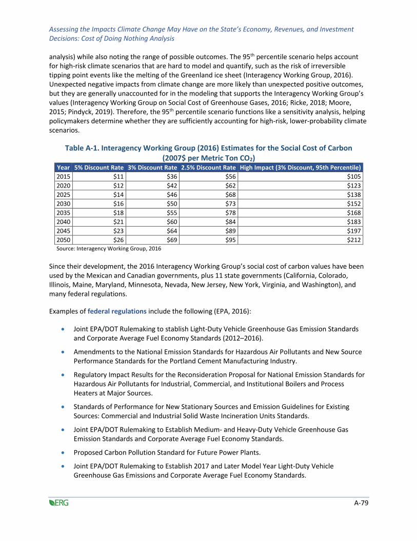
Assessing the Impacts Climate Change May Have on the State’s Economy, Revenues, and Investment Decisions: Cost of Doing Nothing Analysis
A-79
analysis) while also noting the range of possible outcomes. The 95th percentile scenario helps account for high-risk climate scenarios that are hard to model and quantify, such as the risk of irreversible tipping point events like the melting of the Greenland ice sheet (Interagency Working Group, 2016). Unexpected negative impacts from climate change are more likely than unexpected positive outcomes, but they are generally unaccounted for in the modeling that supports the Interagency Working Group’s values (Interagency Working Group on Social Cost of Greenhouse Gases, 2016; Ricke, 2018; Moore, 2015; Pindyck, 2019). Therefore, the 95th percentile scenario functions like a sensitivity analysis, helping policymakers determine whether they are sufficiently accounting for high-risk, lower-probability climate scenarios.
Table A-1. Interagency Working Group (2016) Estimates for the Social Cost of Carbon (2007$ per Metric Ton CO2)
Year 5% Discount Rate 3% Discount Rate 2.5% Discount Rate High Impact (3% Discount, 95th Percentile)
2015 $11 $36 $56 $105
2020 $12 $42 $62 $123
2025 $14 $46 $68 $138
2030 $16 $50 $73 $152
2035 $18 $55 $78 $168
2040 $21 $60 $84 $183
2045 $23 $64 $89 $197
2050 $26 $69 $95 $212 Source: Interagency Working Group, 2016
Since their development, the 2016 Interagency Working Group’s social cost of carbon values have been used by the Mexican and Canadian governments, plus 11 state governments (California, Colorado, Illinois, Maine, Maryland, Minnesota, Nevada, New Jersey, New York, Virginia, and Washington), and many federal regulations.
Examples of federal regulations include the following (EPA, 2016):
• Joint EPA/DOT Rulemaking to stablish Light-Duty Vehicle Greenhouse Gas Emission Standards and Corporate Average Fuel Economy Standards (2012–2016).
• Amendments to the National Emission Standards for Hazardous Air Pollutants and New Source Performance Standards for the Portland Cement Manufacturing Industry.
• Regulatory Impact Results for the Reconsideration Proposal for National Emission Standards for Hazardous Air Pollutants for Industrial, Commercial, and Institutional Boilers and Process Heaters at Major Sources.
• Standards of Performance for New Stationary Sources and Emission Guidelines for Existing Sources: Commercial and Industrial Solid Waste Incineration Units Standards.
• Joint EPA/DOT Rulemaking to Establish Medium- and Heavy-Duty Vehicle Greenhouse Gas Emission Standards and Corporate Average Fuel Economy Standards.
• Proposed Carbon Pollution Standard for Future Power Plants.
• Joint EPA/DOT Rulemaking to Establish 2017 and Later Model Year Light-Duty Vehicle Greenhouse Gas Emissions and Corporate Average Fuel Economy Standards.
Assessing the Impacts Climate Change May Have on the State’s Economy, Revenues, and Investment Decisions: Cost of Doing Nothing Analysis
A-80
Examples of state regulations include the following:
• The State of Maine has already used the Federal Interagency Working Group’s social cost of carbon values in its April 2015 Public Utilities Commission regulation implementing the 2014 Act to Support Solar Energy (LD 1652, 2014). The Commission’s Maine Distributed Solar Valuation Study includes a social cost of carbon estimate alongside other benefits and costs of solar, such as avoided energy costs, transmission capacity benefits, and reduced fuel price uncertainty (Maine Public Utilities Commission, 2015). The Commission uses the 2010 Interagency Working Group social cost of carbon values with a 3 percent discount rate: $52 (2018$) per metric ton of CO2 emitted in 2020. However, because some carbon costs are already embedded in the base energy value due to provider compliance with Regional Greenhouse Gas Initiative carbon allowances, the Commission subtracted the costs of regional carbon allowances from the applicable year of the federal social cost of carbon estimate to arrive at its adjusted social cost of carbon per kilowatt-hour (kWh) value: $0.021. The Commission values the overall benefits of distributed solar at $0.182/kWh in the first year of solar system installation, with the social cost of carbon comprising 28 percent of the total value (Maine Public Utilities Commission, 2015). Maine therefore has precedent for applying existing federal analysis to relevant state policy.
• New York State has used the 2016 federal social cost of carbon values for clean energy standards, emissions credit programs, wholesale energy markets, and statewide agency decision-making since January 2016 (Avallon, 2019).
• The State of New Jersey uses the 2016 federal social cost of carbon values in its Zero-Emissions Credit Program as of May 2018 (S2313, 2018).
• The State of Maryland uses the 2016 federal social cost of carbon values in its 2019 climate action plan and in its November 2018 utility oversight analysis of the benefits of solar power (Maryland Department of the Environment, 2019; Daymark Energy Advisors, 2018).
• As of April 2019, the State of Washington requires that utilities use the 2016 Interagency Working Group social cost of carbon estimate at the 2.5 percent discount rate—$78 per metric ton of CO2 emitted in 2020, codified to rise with inflation—in their integrated resource plans (SB5116, 2019).
• The State of California uses the 2016 federal social cost of carbon values in its November 2017 Climate Change Scoping Plan, and the California Air Resources Board has been required to account for the social costs of greenhouse gases since summer 2016 (California Air Resources Board, 2017).
• In Minnesota, regulations have required utilities to account for the specific environmental costs of various generation methods since 1994. In 2016, Public Utilities Commission procedures updated these requirements to use the 2016 federal social cost of carbon values as “the best available measure” for CO2 (State of Minnesota, 2016; Minnesota Public Utilities Commission, 2017).
• As of August 2018, Nevada law requires that utilities use a global social cost of carbon value in their three-year energy supply plans. The law specifies that this value “must be calculated using the best available science and economics, such as the analysis set forth in the [2016 Interagency Working Group] Technical Support Document” (Nevada Public Utilities Commission Order, 2018).

Assessing the Impacts Climate Change May Have on the State’s Economy, Revenues, and Investment Decisions: Cost of Doing Nothing Analysis
A-81
A.1.2. 2018 Interim Social Cost of Carbon Estimates
In 2017, Executive Order 13783 revoked several previous climate-change-related executive orders, rescinded the implementation of the 2016 Interagency Working Group social cost of carbon values, and disbanded the Interagency Working Group. The executive order further instructed EPA to re-estimate the social cost of carbon based on 2003 guidance from Office of Management and Budget Circular A-4, which emphasizes domestic policy impacts and market-based discount rates (U.S Environmental Protection Agency (EPA), 2018; Office of Management and Budget (OMB), 2003).
In August 2018, EPA published a regulatory analysis with new, interim social cost of carbon estimates (summarized in Table A-2 below), which follow the new administration guidelines. These values represent current federal policy for regulatory analysis, but EPA has not yet published formal technical support documents for the interim values. These new values have not yet been used in state legislation.
Table A-2. Interim EPA (2018) Domestic Social Cost of Carbon, 2015–2050 (2016$
per Metric Ton of CO2) Year 3% Discount Rate 7% Discount Rate
2020 $7 $1
2025 $7 $1
2030 $8 $1
2035 $9 $2
2040 $9 $2
2045 $10 $2
2050 $11 $2 Source: EPA, 2018
Although the 2018 estimates use the same underlying scientific models as the 2016 Interagency Working Group, the 2018 estimates use higher discount rates, do not report the 95th percentile scenarios, and consider only domestic impacts. These choices yield lower social cost of carbon values: $1 and $7 (in 2019$) per metric ton of CO2 emitted in 2020, at 7 and 3 percent discount rates, respectively (EPA, 2018).
The choice to consider only domestic versus global climate impacts is the major difference—other than discount rate—leading to such disparate social cost of carbon estimates. Most peer-reviewed estimates use global impacts because CO2 is an atmospheric pollutant, which affects the global climate system no matter where it is emitted (Pindyck, 2019; Ricke et al., 2018; Revesz et al., 2017; Howard and Schwartz, 2017; Pizer et al., 2014; Wang et al., 2019). National CO2 emissions and climate changes also build on each other cumulatively and interact across borders due to globalized trade, migration flows, and broad ecological impacts. Political theorists recommend using a global social cost of carbon to foster international cooperation and robust climate action (Ricke et al., 2018; Revesz et al., 2017). Furthermore, growing evidence shows that climate change disproportionately impacts countries and populations that emit less CO2, creating an internationally unjust situation if high emitters use a domestic social cost of carbon estimate (Ricke et al., 2018). Scientific literature supports the United States using global social cost of carbon estimates in domestic policy, which would be analogous to state governments taking national and regional impacts into account when creating state policy.

Assessing the Impacts Climate Change May Have on the State’s Economy, Revenues, and Investment Decisions: Cost of Doing Nothing Analysis
A-82
Taken together, restricting the social cost of carbon to domestic impacts, and raising the discount rate to 7 percent, accounts for all of the difference between the 2016 and 2018 federal values. In the appendix to the 2018 analysis, EPA notes that when global costs are included, the social cost of carbon rises to $53 per metric ton of CO2 emitted (2016$) in 2025 using a 3 percent discount rate (EPA, 2018, pg. 7-7). This number is the same as the 2016 Interagency Working Group’s 3 percent estimate of $46 per metric ton of CO2 emitted in 2025, once the figure is converted from 2007 dollars to 2016 dollars (Interagency Working Group, 2016, pg. 4). Thus, the federal estimates actually agree more than they appear to, apart from the differing decisions on discount rate and geographic frame of reference.
Overall, scientists and experts agree that the 2016 Federal Interagency Working Group social cost of carbon values still represent the best available science and economics, as they robustly account for the full international effects of climate change and the high risk of negative climate outcomes (Institute for Policy Integrity, 2017; Revesz et al., 2017, Ricke et al., 2018; Metcalf and Stock, 2015). We use the 2016 Interagency Working Group social cost of carbon values throughout this analysis.
A.1.3. Discount Rates
The 2016 Interagency Working Group presented multiple discount rates (2.5 percent, 3 percent, and 5 percent) so that policy- and decision-makers could select the rate most applicable to their analysis while noting the range of possible outcomes. The 2018 interim EPA guidance uses 3 percent and 7 percent rates. In the relevant scientific literature, we observed discount rates ranging from 0 percent to 5 percent, excluding the 7 percent value that EPA used in 2018 (Adler et al., 2017). A 2019 survey of 200 climate experts and economists found substantial agreement with a 2 to 3 percent discount rate for climate-related cost-benefit analyses (Pindyck, 2019).
Therefore, for this work, we use a 3 percent discount rate, as it closely aligns with the rate that the Efficiency Maine Trust uses, is a common thread between EPA’s 2016 and 2018 guidance, and has robust support from scientific experts.
A.1.4. Social Cost of Carbon Estimates Extrapolated to 2100
The federal social cost of carbon estimates (from both 2016 and 2018) present values for carbon emitted out to the year 2050. To extrapolate the 2016 federal 3 percent and 95th percentile estimates out to 2100, we conducted a linear regression that yielded a social cost of carbon of $140 and $442 per metric ton of CO2 emitted in 2100, respectively, in 2019 dollars (see Table A-3).
Table A-3. 2016 Interagency Working Group High and Low Social Cost of Carbon Values Extrapolated to 2100
Social Cost of Carbon
Year Original Low-Bound Values (3%, 2007$)
Extrapolated Low-Bound Values (3%, 2019$)
Original 95th Percentile Values (2007$)
Extrapolated 95th Percentile Values (2019$)
2020 $42.00 $51.02 $123.00 $149.41
2025 $46.00 $55.88 $138.00 $167.63
2030 $50.00 $60.74 $152.00 $184.64
2035 $55.00 $66.81 $168.00 $204.07
2040 $60.00 $72.88 $183.00 $222.29
2045 $64.00 $77.74 $197.00 $239.30
2050 $69.00 $83.82 $212.00 $257.52
2100 Not given $139.82 Not given $441.99

Assessing the Impacts Climate Change May Have on the State’s Economy, Revenues, and Investment Decisions: Cost of Doing Nothing Analysis
A-83
Note that this extrapolation assumes that the economic and climate trends modeled in the Interagency Working Group’s analysis through 2050 will hold until 2100. The uncertainty of climate projections and economic scenarios increases later in the century. Slower economic growth rates expected from climate change also lower the appropriate discount rate over time, which would lead to a higher social cost of carbon than the extrapolated values listed.
Nonetheless, our extrapolated values generally align with the scientific literature that estimates the social cost of carbon out to 2100. Several peer-reviewed analyses used the same integrated climate models as the Interagency Working Group but improved and extended the models to estimate damages out to 2100. These long-term calculations display a wide range of uncertainty but generally align with the high and low bound of $140 and $442 arrived at via extrapolation.
Cai and Lontzek (2019) use large-scale computing to model the probability of various climate and economic pathways. This is a more sophisticated approach than the typical use of pre-determined, simplified modeling inputs. In Cai and Lontzek’s benchmark case with middle-ground economic assumptions, the median social cost of carbon is $78 per ton of CO2 in 2100, but with a 10 percent chance of exceeding $191 per ton of CO2 and a 1 percent chance of exceeding $327 per ton of CO2 (pg. 5). Their average expected social cost of carbon in 2100 is $126 per ton of CO2 in 2019 dollars, which aligns with our low-bound extrapolated estimate of $140. Note that in Cai and Lontzek’s published paper, they report their estimates per ton of carbon, which is about three times as large as the social cost of carbon per ton of CO2. We have converted the estimates here for ease of comparison.
Moore and Diaz (2015) extend the Interagency Working Group’s models to determine the expected impact of high temperatures on economic growth rates, rather than just economic levels. They find a global social cost of carbon of $350 per ton of CO2 emitted in 2100 under their DICE-2R model, which differentiates economic impacts from temperature on wealthy versus poorer regions (pg. 128). Their alternate model, gro-DICE, assumes strong adaptation activities but also includes high temperatures that affect total factor productivity, leading to even larger social cost of carbon values. These values peak at $900 per ton of CO2 by 2080 before lowering to about $500 in 2100, with a range of uncertainty as high as $1,500 in 2080 and $1,200 in 2100, all given in 2015 dollars (pg. 128). These estimates align with or exceed our high-bound extrapolated estimate of $442 in 2100.
Yang et al. (2018) model the social cost of carbon out to 2100 using the five shared socio-economic pathways published by Riahi et al. (2017). The pathways are robust scenarios that predict likely economic growth rates based on geopolitical interactions, such as the presence or absence of international cooperation regarding mitigation. Yang et al. find a social cost of carbon range of $10 to $1,192 per ton of CO2 by 2100 across all five pathways and all damage functions at a 1.5 percent discount rate, with a mean of $157 by 2100 and moderate damage assumptions. Under pathway five, where developing countries follow the same path as historical industrializations, they find a social cost of carbon of $471 per ton of CO2 by 2100, with moderate damage assumptions. That rises to $864 per ton of CO2 by 2100 with sharp damage functions. Note that these estimates use a lower discount rate (1.5 percent), so they are somewhat inflated compared to estimates of the social cost calculated using a 3 percent discount rate. At a 3 percent discount rate, Yang et al.’s values would likely fall in the middle of our extrapolated range for the social cost of carbon in 2100.
As these disparate estimates show, a wide range of uncertainty is involved in estimating the social cost of carbon out to 2100. Nonetheless, by extrapolating the 2016 Interagency Working Group’s low- and high-bound values out to 2100, we arrive at a low and high bound of $140 and $442 per ton of CO2

Assessing the Impacts Climate Change May Have on the State’s Economy, Revenues, and Investment Decisions: Cost of Doing Nothing Analysis
A-84
emitted in 2100, which approximately matches the range of social cost of carbon estimates for 2100 in the relevant literature.
A.2. MARKET PRICE OF CARBON
The market price of carbon provides an alternative mechanism to value carbon emissions reductions, distinct from the social cost of carbon approach detailed in Section A.1. Rather than valuing carbon emissions based on social and environmental factors, the market approach prices carbon emissions based on the cost of regulatory compliance, as if emissions are market goods. The most relevant source of market carbon pricing for Maine is New England’s Regional Greenhouse Gas Initiative, which Maine joined in 2007.
The Regional Greenhouse Gas Initiative was established in 2005 as the first market-based program in the United States seeking to reduce greenhouse gas emissions, and it is composed of 10 Northeast and Mid-Atlantic states, including Maine (Regional Greenhouse Gas Initiative, 2020). The Regional Greenhouse Gas Initiative does not publish projections or estimates of the market price of carbon out to 2050. However, information from past regional pricing can help predict future market prices.
In 2018, the State of New Jersey (also a member) forecasted the market price of carbon from 2016 to 2030 to help evaluate different carbon reduction activities. Synapse Energy Economics, subcontractor to ERG, extrapolated these carbon prices and forecasted the market price of carbon through 2050. Table A-4 summarizes these extrapolated market values. See Table A-5 for a comparison between the market values and the broader, higher social cost of carbon values.
Table A-4. Forecast of the Market Price of Carbon Based on Regional Greenhouse Gas
Initiative Price Projections
Maine Forecast
Year Nominal $/Short Ton 2018$ /Short Ton
2020 $5.61 $5.43
2025 $5.54 $4.94
2030 $7.02 $5.78
2035 $8.90 $6.75
2040 $11.27 $7.88
2045 $14.28 $9.21
2050 $18.10 $10.76
A.3. RECOMMENDATIONS FOR MAINE
To monetize carbon emissions, we recommend that the State of Maine adopt the social cost of carbon values from the 2016 Interagency Working Group analysis, using the 3 percent discount rate and the 95th percentile outcome as low and high bounds. Those scenarios yield a social cost of carbon ranging from $51 to $150 (2019$) per metric ton of CO2 emitted in 2020 and $84 to $258 (2019$) per metric ton of CO2 emitted in 2050 (Interagency Working Group, 2016). Extrapolating those values out to 2100 yields a low and high bound of $140 and $442 (2019$), respectively, per metric ton of CO2 emitted in 2100. These values approximately match the range of estimates in the scientific literature, although with a high degree of uncertainty.

Assessing the Impacts Climate Change May Have on the State’s Economy, Revenues, and Investment Decisions: Cost of Doing Nothing Analysis
A-85
Table A-5. Summary of Social Cost of Carbon Versus Market Price of Carbon, Extrapolated to 2100
Year Lower Bound Social Cost of Carbon in 2019$ (EPA, 2016)
Upper Bound Social Cost of Carbon in 2019$ (EPA, 2016)
Market Price of Carbon in 2019$ (Synapse, 2020)
2020 $51.02 $149.41 $5.53
2025 $55.88 $167.63 $5.03
2030 $60.74 $184.64 $5.88
2035 $66.81 $204.07 $6.87
2040 $72.88 $222.29 $8.02
2045 $77.74 $239.30 $9.37
2050 $83.82 $257.52 $10.95
2100 $139.82 $441.99 $51.83
Rather than being an outlier, the 95th percentile outcome helps align the federal social cost of carbon values with the body of relevant, peer-reviewed scientific literature, which frequently returns a noticeably higher social cost of carbon than the middle-ground federal values (3 percent discount rate). Using both the low- and high-bound estimates helps policymakers reflect the full range of climate risks, possible scenarios, and mitigation benefits according to the best available science (Institute for Policy Integrity, 2017; Revesz, 2017; Ricke, 2018; Metcalf, 2015).
The market price of carbon is lower and does not reflect the full range of expected costs from climate change. This report provides results calculated using the market price of carbon for additional context, but these results should not be the primary method of valuing carbon emissions reductions. Overall, we recommend that the State of Maine use the 2016 federal high and low estimates of the social cost of carbon in climate policy analysis.