assessing riparian condition and prioritizing...
TRANSCRIPT
ASSESSING RIPARIAN CONDITION AND PRIORITIZING LOCATIONS FOR STREAMSIDE
REFORESTATION PROJECTS: NORTHERN MANABÍ PROVINCE, ECUADOR
by
Jeremiah A. Jolley
Dr. Jennifer Swenson, Advisor
May 2013
Masters Project submitted in partial fulfillment of the requirements
for the Master of Environmental Management/Master of Forestry degrees in the
Nicholas School of the Environment of
Duke University
2013
ABSTRACT
ASSESSING RIPARIAN CONDITION AND PRIORITIZING LOCATIONS FOR STREAMSIDE REFORESTATION PROJECTS: NORTHERN MANABÍ PROVINCE, ECUADOR
by
Jeremiah A. Jolley
May 2013
Riparian corridors perform ecological functions to a degree that vastly exceeds their spatial
area on the landscape. These unique ecotones decrease sedimentation, provide unique wildlife
habitat, help attenuate flood waters, and improve stream water quality by regulating and absorbing
nutrient and pollutant flows across system boundaries. However, human actions at the landscape
scale are a primary threat to the integrity of river ecosystems. This project focuses on maximizing
ecological benefits through effective riparian restoration planning within one of the world’s most
threatened biodiversity hotspots: the coastal semi-deciduous, tropical dry forests of northwestern
Ecuador. In order to meet the restoration objectives in a cost-effective manner, satellite remote
sensing and geospatial modeling were employed to (a) understand relationships between land
use/land cover (LULC) and drinking water quality across four watersheds of varying sizes and
levels of forest-to-pasture conversion; (b) accurately identify potential restoration sites along
important riparian corridors; and (c) prioritize and recommend restoration sites using a rank
system that focuses on restoration feasibility and the potential to improve water quality, hydrologic
functioning, and wildlife habitat.
Within the four coastal watersheds in the study area, the severity of deforestation ranges
from 24% to 50% mainly due to conversion to pasture for livestock production. This type of land
use change further increases by as much as 10% for areas closest to higher order streams showing
an increased threat to riparian zones. The substantial loss of riparian forest cover led to the
identification of 1,668 potential restoration sites, with an average size of 0.2 ha. Of these potential
sites, 3.8% ranked as “high” priority, 47.6% ranked as “moderate” priority and 48.6% ranked as
“low” priority. Those sites that are ranked the highest priority for reforestation efforts are larger in
size, maximize core-area/edge ratios for prospective wildlife habitat improvements, and have the
best potential to enhance riparian buffer functioning once restored.

ACKNOWLEDGEMENTS
I am extremely thankful to all those individuals who provided advice and support of this
project; especially, thanks to my graduate advisor, Dr. Jennifer Swenson, the staff of the Ceiba
Foundation for Tropical Conservation, my friends, family, and most notably my wife, Allison for her
incredible patience. Also, this project would not have been possible without the SPOT5 image grant
from Planet Action (©CNES (2011), distribution Spot Image S.A.) and the financial support from the
Nicholas School Internship Fund, the Lazar/KLN Foundation, and the SIDG Travel Grant.
TABLE OF CONTENTS
Section Page
1 INTRODUCTION …………………………………………………………………………………………… 1
Historical Land Use in Western Ecuador ………………………………………………. 1
Riparian Corridor Significance……………………………………………………………… 3
Land Use, Water Quality, and Human Health in the Tropics …………………… 5 2 MATERIALS AND METHODS .……………………………………………………………………… … 7 Study Area ………………………………………………………………………………………….. 7 Water Quality Sampling ………………………………………………………………………. 9 Land Use / Land Cover Mapping ………………………………………………………… 13 Digital Elevation Model …………………………………………………………………….... 17 Land Use/ Land Cover Metrics ………………………………………………………….... 18 Site Identification ………………………………………………………………………………. 19 Site Prioritization ………………………………………………………………………………. 23 Final Prioritization Ranking ……………………………………………………………….. 27 3 RESULTS ………………………………………………………………………………………………………. 27 General Land Use, Land Cover Characteristics ……………………………………… 27 LULC Map Accuracy Assessment …………………………………………………………. 28 LULC Summary: Catchment Scale ………………………………………………………... 30 LULC Summary: Stream Network Scale ………………………………………………...31 Land Use Impacts on Water Quality …………………………………………………….. 35 Identification of Potential Restoration Sites …………………………………………. 37 Prioritization of Potential Restoration Sites …………………………………………. 39 4 DISCUSSION …………………………………………………………………………………………………...42 Interpretation of Results ……………………………………………………………………... 42 Use and Limitations of Watershed Restoration Planning ………………………..44 5 RECOMMENDATIONS & CONCLUSION …………………………………………………………...47 Riparian Restoration Management Guidelines ……………………………………….47 Water Quality Data Collection ……………………………………………………………....48 Additional GIS Data Collection ……………………………………………………………...48 Conclusion ………………………………………………………………………………………….. 49 6 REFERENCES ……………………………………………………………………………………………….....50 7 APPENDIX ……………………………………………………………………………………………………...54
1
1. INTRODUCTION
Historical Land Use in Western Ecuador
Decades of deforestation throughout western Ecuador due to timber harvest, shrimp
farming, crop production, and cattle ranching have left a highly diverse set of ecoregions on the
brink of collapse (Southgate and Whitaker 1992, Sierra and Stallings 1998, Wunder 2001,
Economist 2003, López et al. 2010). Mangrove forests, lowland wet forests, dry forests and
montane forests once dominated the landscape westward from the Andes range to the Pacific
Ocean. Of the ecosystems most in peril is the tropical dry forest. Less than 1% of primary dry
forests remain in disparate parcels stretching from the northwest coast in southern Esmeraldas
province towards the central coast in Guayas province and south to Peru, making it one of the most
endangered tropical ecosystems on the planet (Dodson and Gentry 1991).
There are, of course, several different types of dry forest along Ecuador’s coastline resulting
from climactic effects of major ocean currents and elevation gradients. This study focuses on the
transitional, semi-deciduous tropical forests that lie near the equator which are geographically
unique in that they connect the world’s wettest forests in the Chocó of southwestern Columbia to
Ecuador’s true dry forests further south. Floral and faunal residents from the northern rainforests
and southern dry forests make their home in these coastal watersheds creating a dynamic, rich
biodiversity hotspot with high levels of endemism.
As a response to high deforestation rates of 198,000 ha/year country-wide (Sanchez 2006)
and lingering rural poverty, the government of Ecuador instituted a national program in 2008,
called Socio Bosque, to help protect the country’s remaining forests through direct payment
incentives to landowners . In order to determine the priority regions for conservation, the plan
called for a ranking scheme that focused on three main factors: a.) threat of deforestation; b.) the
significance of ecosystem services: carbon storage, biodiversity habitat, and water cycle regulation;
c.) poverty levels (de Koning et al. 2011). The resulting prioritization map characterized the
remaining transitional dry forests in Manabí province in the highest priority category. This
designation aligns with the historically famous prioritization of the world’s most threatened
biodiversity hotspots by Norman Myers (Myers 1988). Myers prioritized highly biodiverse and
rapidly deteriorating hotspot biomes in the late 1980’s. Due to this region’s high rates of
deforestation that was threatening the existence of incredible flora/fauna diversity and endemism,
2
Myers ranked western Ecuador as one of the top biodiversity hotspots; second only to Madagascar
(Myers 1988, Myers et al. 2000).
The Ceiba Foundation for Tropical Conservation (CFTC)1 has been involved in conservation
efforts in this part of the coast since 2001. CFTC aspires to create a biological corridor with the
remaining old growth and mature secondary forests along a 50 km stretch between the coastal
ports of Pedernales and Jama through the creation of private reserves or through protection under
the government’s new payment for ecosystem services (PES) program: Socio Bosque. Ceiba began
a partnership with Socio Bosque at its inception in 2008 and has since enrolled 5100 ha of forested
land into the conservation program, which accounts for nearly 20% of their proposed corridor
(Woodward and Meisl 2010). Despite recent successful efforts on the ground to help protect these
last remnants, few studies are being carried out to explore the incredible biology of these forests
and how the dynamic land-use transformation in this area affects human health, natural resources,
biodiversity, and regional climate change.
The coastal plain of Ecuador is the agricultural backbone of the country. Nearly all the
native mangrove forests have been converted to aquaculture ponds while the humid and dry
forests transitioned into cropland, palm plantations, banana plantations, or most commonly into
pasture for livestock production. In northern Manabí Province, coastal watersheds have been
compromised over the last 40+ years due to increased sedimentation after logging, loss of riparian
buffers, fecal contamination from livestock, and agrochemical pollution run-off (Diario 2009,
Guerrero 2010). These effects have not been effectively quantified to-date and it is likely that time
and natural ecosystem recovery mask the historical interactions between land use conversion and
water quality; however, current qualitative observations in the region by both conservationists and
local residents have prompted action to address the links between land use/land cover (LULC),
water availability, and water quality. In particular to Canton Jama, a county within Manabí
Province, the current emphasis on watershed functioning and water quality stems from local
communities’ concerns about heightened water-borne disease breakouts within various towns.
Residents here rely on water drawn from local streams for drinking, cooking, bathing, and
small-scale farming. Land conversion from forest to pasture often creates riparian gaps where
forest has been cleared right up to stream channel itself. Without a functional riparian forest buffer
between adjacent cattle pastures and streams, various water quality pollutants (e.g. fertilizer, fecal
coliform bacteria from cow manure, and eroded topsoil) can easily enter water channels and
1 www.ceiba.org
3
contaminate local water supplies. The restoration of these degraded streamside riparian zones is
critical for both local stakeholders’ health, re-establishing quality stream habitat for benthic
communities, and for providing corridor connectivity for some of the most protected and oldest
forest patches remaining in Manabí Province.
Riparian Corridor Significance
Riparian corridors perform ecological functions to a degree that vastly exceeds their spatial
area on the landscape. These unique ecotones serve as the interface between terrestrial and
aquatic ecosystems, thus creating one of the most dynamic zones within a landscape (Swanson et al.
1988, Gregory et al. 1991). Among their many services they decrease sedimentation, provide
unique wildlife habitat, help attenuate flood waters, provide steam bank stability, and improve
water quality by regulating and absorbing nutrient and pollutant flow across system boundaries
(Gregory et al. 1991, Allan 2004, Baker et al. 2006). However, human actions at the landscape scale
are a primary threat to the integrity of river ecosystems especially if land use change occurs within
the riparian zone. There are numerous environmental factors that can affect aquatic systems, yet
the presence of a factor is rather dependent on the level of development for a given country or
specific sub-region of a country. For example, waterways in highly industrialized Western
countries experience a higher threat of exposure to nutrient enrichment, heavy metals, synthetics,
and toxic organics. Hydrologic alteration due to creation of levees, dams, roads, and urban
development also occurs much more commonly in such regions. Within the context of the remote
coastal regions of Ecuador, the main environmental factors that degrade river ecosystems and
streamside buffer functioning are riparian clearing/canopy opening, a loss of coarse woody debris,
and sedimentation from cropland and cattle pasture.
The amount of solar radiation reaching a stream channel, and thus potential for significant
increases in water temperature, is a function of both stream channel width and the structure and
composition of riparian vegetation (Gregory et al. 1991). Because the vast majority of stream
reaches within this study area do not exceed 10 m in width, significant shading occurs where
riparian zones are intact and have not been cleared. Riparian vegetation cover then becomes the
dominant factor in influencing stream temperatures. A study in Ontario found stream temperature
to be the only variable that clearly explained streams with and without healthy trout populations
(Barton et al. 1985). Barton et al. further determined that stream temperature maximum means
were inversely correlated to stream bank forest cover upstream from sampling sites. That is, less
4
forest cover within a distance of 2.5 km upstream led to significantly increased water temperatures.
Deforestation of riparian canopy clearly alters stream water temperature in an intuitive manner.
However, Bourque and Pomeroy (2001) have shown that clear cut timber harvesting outside of
forest buffer zones can also raise summer mean stream temperatures by 4-8% in catchments even
when riparian forested areas (30-60 m) have not been impaired at all. In other research, the loss of
riparian canopy has also been linked to decreases in bank stability and retention of
pollutants/nutrients (Lowrance et al. 1984, Osborne and Kovacic 1993, Martin et al. 1999),
alteration of organic carbon reaching streams (Findlay et al. 2001), and impacts on
macroinvertebrate and fish community composition (Stauffer et al. 2000).
The presence of riparian trees within streamside buffer strips allows for consistent sources
of coarse woody debris (CWD). Trees that fall across streams and within riparian zones help to
retain water and organic material (e.g. leaves, branches, wood), store sediments and enhance
biological productivity within river ecosystems (Ehrman and Lamberti 1992, Gurnell et al. 1995,
Maridet et al. 1995). CWD also provides a substrate for feeding, attachment and cover for benthic
organisms (Johnson et al. 2003).
The loss of forest in any area of a watershed, whether in the riparian zone or not, exposes
previously protected soil to surface runoff forces following rain events. Fine soil particles are
picked up and flow across surface pathways where they eventually end up in streams and
contribute to the confounding problem of sedimentation. Significant positively correlated
relationships have be found between the extent agricultural land use within a catchment and
various measures of sediment load including suspended solids, bedload, and substrate
embeddedness (Wood and Armitage 1997, Quinn 2000, Sutherland et al. 2002). Although
sedimentation is a naturally occurring process, human induced sediment deposition occurs on a
scale that lowers habitat quality for aquatic biota. For example, suspended sediment has been
shown to lower the reproductive success of tricolor shiner, Cyprinella trichroistia (Burkhead and
Jelks 2001) and mainstream reaches with high sediment loads that drained agricultural lands
significantly reduced fish diversity in the central Chattahoochee River (Walser and Bart 1999).
From a watershed management perspective, there is clear evidence for the myriad ecological
services which riparian zones provide. The preservation and restoration of these unique ecotones
will serve to benefit humans, riverscapes, and landscapes alike.
5
Land Use, Water Quality, and Human Health in the Tropics
Stream ecosystems are highly impacted by human land use at different spatial scales. Such
impacts are usually measured in various physical, chemical, and biological metrics that represent
varying degrees of water quality or habitat condition. Within the literature, results vary between
studies that explore relationships between land use and these numerous stream response
indicators (Allan 2004). The matrix of geomorphological traits, natural vegetation cover, soil
substrate, land use alteration and levels of spatial analysis (catchment-wide, stream network, and
local reach) must be kept in mind when drawing conclusions from a particular study. This section
aims to explore research within tropical ecoregions that focus on the impairment of drinking water
quality and riparian condition due to land use change.
Stream ecologists will often sample macroinvertebrate organisms and then calculate a
biotic index as an indicator of water quality because certain species are more sensitive to
suspended solids, temperature, and pollutants than others (Fenoglio et al. 2002, Figueroa et al.
2003). This index is one of the most commonly used biological metrics and is usually shown to be
negatively correlated with agricultural land use and positively correlated with forest cover in the
riparian zone (Wang et al. 1997, Miserendino et al. 2011). In the Ecuadorian Amazon, Bojsen and
Jacobsen (2003) found that both alpha and beta diversity of macroinvertebrate communities
decreased at sites with deforested riparian areas as compared to those sites that were forested.
Changes in trophic structure occurred in deforested sites as overall macroinvertebrate abundance
increased with a higher relative density of collectors, but lower density of predators. A similar
study in Costa Rica determined that riparian forest buffers of at least 15 m can mitigate the loss of
macroinvertebrate diversity due to deforestation (Lorion and Kennedy 2009). In addition to
riparian land cover metrics, impaired structure and composition of macroinvertebrate assemblages
have also been shown to correlate with physical and chemical indicators of degraded water quality
(Buss et al. 2004, Soldner et al. 2004).
Other studies have collected indicator data to examine hydrobiogeochemical changes in
stream ecosystems. For example, Figueiredo et al. (2010) examined whether cation/anion loads
and chemical water properties (pH, turbidity, dissolved oxygen, water temperature) in small
streams were affected by deforestation and increased agriculture use in eastern Amazon. They
found that the simplest indicators appeared most useful in detecting effects of land use change;
particularly, forest cover. For five streams in the Amazon, they determined stream temperature,
dissolved oxygen, pH and turbidity are better indicators than biochemical concentrations of cations
(Ca2+, Mg2+, K+, Na+) and anions (Cl-, NO3-, SO42-).
6
Certain water quality indicators correlate with land use/land cover (LULC) at different
spatial scales. Using a historical 23-year water quality dataset from Puerto Rico, Uriarte et al.
(2011) reported that turbidity and DO responded to LULC at the catchment-wide scale, while fecal
coliform concentrations responded best to LULC and the sub-watershed scale. Fecal contamination
in streams through soil leaching is one of the biggest human health concerns for rural communities
in Canton Jama. While specific studies have not been carried out in Jama, the high prevalence of
enteroinvasive Escherichia coli has been documented further up the coast in similar rural regions
(Vieira et al. 2007). Additional work in the Seine watershed found that streams flowing through
areas partially or completely covered with grazing pasture experienced high loads of fecal bacteria
and other suspended solids (George et al. 2004). Increased rainfall further added such
contaminants in to local streams. Given the large percentage of pastureland and high rainfall
during the wet season in Jama, there is great potential to help improve water quality and reduce
water borne disease incidents through reforesting riparian buffer zones.
This project focuses on maximizing ecological benefits through effective riparian
restoration planning within one of the world’s most threatened biodiversity hotspots: the coastal
semi-deciduous, tropical forests of northwestern Ecuador. In order to meet the restoration
objectives in a cost-effective manner, several field and digital geographic datasets were either
collected or created using remote sensing and geospatial modeling, and then analyzed to (a)
measure water quality across watersheds of varying sizes and levels of deforestation; (b)
understand relationships between land use/land cover (LULC) and drinking water quality in this
particular ecosystem; (c) accurately identify potential restoration units along important riparian
corridors; and (d) prioritize and recommend restoration units that will maximize riparian buffering
capacity and reduce the threat of water-borne diseases for local communities.

7
2. MATERIALS & METHODS
Study Area
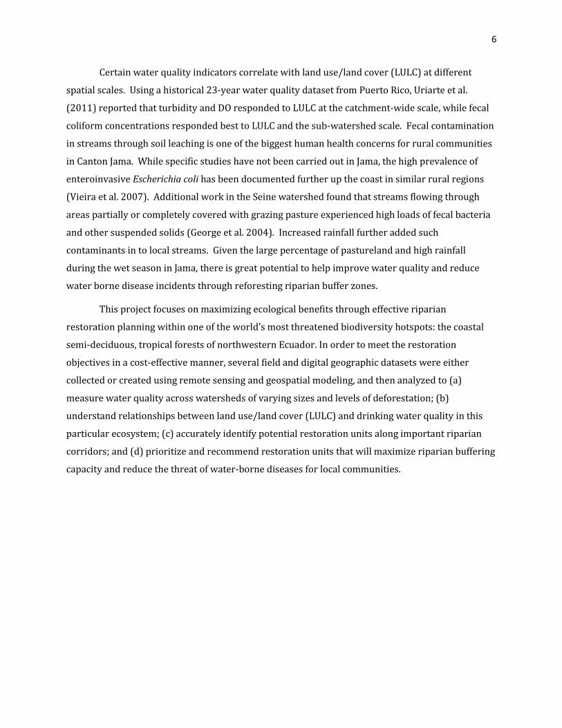
The province of Manabí is located on the northwest coast of Ecuador whose latitudes extend
above and below the equator. The study area in question comprises 4 small watersheds within a
county of Manabí Province called Canton Jama ( 0°3’18 – 0°14’0 S, 80°6’0 - 80°14’11 W, see Figure
1). Each watershed is named after the rural communities (<800 persons) that exist near the
mouths of the main streams’ channel outlet into the Pacific Ocean. The most northward watershed
is Tabuga, followed southward by Camarones, Tasaste, and Don Juan. Three of the catchments
encompass <3,000 ha; however, Don Juan is 8,613 ha and is larger than the others combined.
Canton Jama lies directly in the middle of the transition zone that links Ecuador’s driest
tropical forests to the south with the famously wet Chocó rainforests of northwest Ecuador and
southern Columbia. The cold Humboldt Current runs up the coast from Chile and Peru bringing dry
conditions, whereas the Panama Current travels southward bringing warm waters and moist air.
This forest transition zone occurs in the regions just north and south of the equator due to the
merging and seasonal northward and southward oscillation of these two major ocean currents. As
a result, the transitional coastal forests experience a gradient from drier to more humid conditions
as you move northward in latitude from 1° S (Dodson and Gentry 1991). There is also an elevation
gradient that roughly defines various forest cover types generally referred to by the following
classes: 1.) tropical deciduous vegetation is found down in coastal plains to 100 m above sea-level;
2.) moist semi-deciduous forests are located roughly between 100-300m; and 3.) upper elevations
(300 – 700 m) transition into evergreen, broadleaf montane forests (Neill 1999, Sierra 1999, Figure
1). Dry seasons are variable but typically span from June to the end of November or early
December. However, consistent cloud cover help mitigate effects from high temperatures and
dryness during this period. Annual precipitation yields anywhere from 1,500 mm to 3,000 mm,
with a minimum monthly rainfall of 10mm (Dodson and Gentry 1991, Neill 1999).
8
Figure 1. Map of Study Area: Northern Manabi Province, Ecuador
9
The predominant land use in the region is grassland pasture for cattle grazing. The vast
majority of all old-growth forests were first selectively logged for high value timber and then cut,
burned and converted to pasture since the mid 1970’s (Sierra and Stallings 1998, Wunder 2001,
López et al. 2010). Some land-use has altered between pasture and cropland but this occurs on
rather small scales for subsistence farming. Remaining forest patches are found at higher
elevations where steep slopes prove difficult for successful cultivation or livestock management.
Canton Jama and Canton Pedernales hold most of the last remnants of pristine montane and
deciduous forest along this part of the coastal cordillera (mountain range). The presence of several
intact, neighboring forest patches is a significant reason why the Ceiba Foundation for Tropical
Conservation continually works towards protection of these few watersheds with an end goal of
establishing a connected forest corridor.
Water Quality Sampling
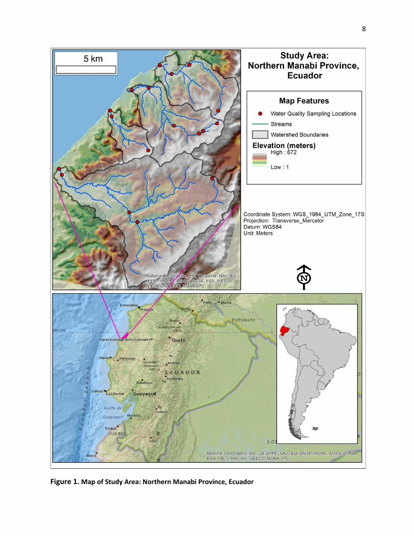
A total of 18 water quality sampling locations were chosen across the study area: 4 in
Tabuga, 6 in Camarones, 3 in Tasaste, and 5 in Don Juan (Figure 2). The initial standards for site
selection were determined by catchment size and the proximity of local towns to the coastline. At a
minimum, each watershed was sampled at the headwaters of the main channel, upstream of town,
downstream of town, and at a final drainage point near the end section of the riverine system.
However, the towns of Tasaste and Don Juan are situated around the mouth of their respective river
and thus the post town sampling site was also the final drainage site. The larger watersheds were
also sampled at major forest/pasture boundaries or after the confluence of another major tributary.
This assured that we could assess impacts of deforestation, grazing, as well as inputs from human
development. All sites needed to be outside of tidal influence, have a length of 100m and contain at
least two types of macroinvertebrate habitat. Headwater sites were chosen as the furthest point up
the main channel that had deep enough pools for adequate data collection. Local guides (usually
the landowner) were hired to find difficult to reach headwater sites.
10
Figure 2. Water Quality Sampling Locations. There are 18 sites in total: 4 in Tabuga, 6 in Camarones, 3 in Tasaste, and 5 in Don Juan
11
It has long been known and investigated that the health of stream ecosystems are
threatened by land use change within its catchment; in particular due to anthropogenic activities
(Allan 2004). There are a variety of source indicators of water pollution that can be tested to
characterize the condition of a given watershed. Our water sampling procedures were based on
Wisconsin’s Water Actions Volunteers Network citizen science program but included modifications
to adjust for local ecosystem characteristics (WAV 2011) . In addition to basic hydrogeochemical
indicator data, we recorded data for preliminary benthic macroinvertebrate surveys, fecal coliform
bacteria surveys, and qualitative riparian habitat condition assessments. Such sampling does not
require expensive monitoring equipment or the necessary laboratory sample analysis that is
needed for nutrient concentration measurements. All water quality parameters can be calculated in
the field, except for fecal coliform colony counts. Overall, this sampling method followed a simple
approach that allows local citizens to monitor their local fresh water systems.
Temperature: Air and water temperature were measured with both regular thermometers
as well as a digital, hand-held YSI Dissolved Oxygen meter.
Dissolved Oxygen (DO): Levels of DO (% saturation and mg/L) were recorded using a YSI
Dissolved Oxygen Meter. We also sampled with Hach Dissolved Oxygen test kits when
working with community members because this will be the preferred method for future
data collection. These kits are simple and economical by utilizing drop count titration
procedures.
Stream Flow/Volume: JDC’s Flowatch air/liquid flow meter was used for measuring
stream discharge velocity. Using the basic concept of distance/time = velocity, we also
assessed stream flow by marking a measured distance and recording the amount of time it
takes a tennis ball to pass through that section. Discharge volume was calculated using the
average stream velocity measurement and the cross-sectional area of a given sample site.
Baseflow at headwater sites often proved insufficient for this measurement.
Biotic Index: Three subsamples of macro-invertebrates were collected for each water
quality station; two from habitats of highest biodiversity (ie. cobblestone riffles) and one of
less diversity (ie. undercut logs, leaf packs). The samples were then combined to survey the
species diversity and richness. Being that no investigations have been performed on the
freshwater aquatic life in the central and north coast of Ecuador, we have not yet calculated
biotic index. Classifications were performed at the level of Order using field guides from
Wisconsin benthic macro-invertebrate studies. Samples from this study were taken to the
University of San Francisco, Quito (USFQ) in 2011 which generated interest to further
12
investigate aquatic stream ecology on the coast. There are current preparations being made
to implement a study solely focused on identifying aquatic organisms from streams along
the coast in Manabi Province to provide a more applicable biotic index scoring assessment
for stream health.
Habitat Assessment: This method was adapted from the Wisconsin WAVN to quantify a
visual assessment of overall stream and riparian health. There are 10 factors which, when
rated on a scale of 1-4 (each rating magnitude has a detailed description which lessens
subjectivity), give an overall habitat score. The factors are: riparian vegetation, bank
vegetation, bank stability, channel alteration, channel flow status, stream velocity/depth, in-
stream fish habitat, sediment deposition, embeddedness, and attachment sites for macro-
invertebrates. The higher the score, the better the site is considered to support wildlife.
Turbidity: We employed a 120cm turbidity tube to measure the amount of suspended
solids (transparency) in the stream for a given site. The tube was first filled with
undisturbed water, and then water was released from the tube until the secchi disk at the
lower end became visible while looking downward through the water column from above.
The length of the tube is marked in cm and the water level was recorded. Multiple trials
were taken for an average. Normally, turbidity is measured in NTU units where a higher
number corresponds to a great magnitude of suspended solids in the sample. However,
when turbidity is measured in cm, a lower number corresponds with the water sample
being more turbid. A high measurement (> 100cm) represents very clear and transparent
water.
E. Coli sampling: All water samples were taken mid-water column and stored in whirl-
packs within a cooler. Upon returning from the field, 1 mL of water sample was placed on a
3M Petrifilm petri plate for each sampling location. The plate was then incubated at 35°C for
24 hours and 48 hours. Blue colonies were counted after each period to note discrepancies
between incubation periods. Fecal coliform numbers are represented in colony forming
units (CFU) / 100 mL. Samples that could not be plated and incubated immediately
following field collection were stored in a refrigerator for a maximum of 1-2 days to restrict
bacteria growth.
13
Land Use/ Land Cover Mapping
Prior to this study, there was a lack of high or even medium quality digital geographic
information for this remote region of Ecuador. The country’s national land cover, climate, soils,
hydrology, terrain, ecotone, and species distributions maps only exist in coarse 1km resolution. For
a study area as small as 150 km2, it is not worthwhile to perform any geographic based analyses at
this level of resolution. While specific studies of improved detail have been carried out in other
focused regions of the country, the application of remote sensing and landscape modeling has yet to
take hold in ecological investigations within Canton Jama, Manabí. I used ENVI 4.8 and 5.0 software
for image processing and Arc-GIS 10.1 for geospatial modeling.
Satellite Image Preprocessing
One of the principal goals for this project is to accurately characterize and map riparian
corridors both in terms of geographic location and vegetation cover within those corridors. On a
landscape scale, the utilization of satellite images gives resource managers a convenient method to
assess land cover characteristics. If the satellite sensor has high enough spatial resolution, then it is
possible to also manually define stream channels for riverine systems of higher order. However, it
is important to understand the benefits and limitations of remotely sensed data and to match the
spatial, temporal, and spectral resolution of a particular satellite sensor to fit the needs of a given
study area (Chuvieco and Huete 2009). I chose to use SPOT5 images as the basis for creating my
land cover classification for 3 reasons: (1) the spatial resolution of 10 meters provides highly
improved vegetation class separation along riparian corridors as compared to the traditional 30 m
Landsat images; (2) the green, red, and near infrared bands are most suitable for distinguishing
ground cover reflectance values of varying vegetation types; (3) the acquired images contained
minimal cloud cover for the majority of the study area, especially in low-lying areas where forest
cover is the most fragmented.
The two base images for my analysis came from a Planet Action2 project grant. The Planet
Action program is an initiative of Spot Image3 to provide geographic information and technology for
support of landscape studies having a link to climate change as a result from anthropogenic land
use change. In order to generate a cloud free LULC classification map across the 4 watersheds, I
processed four separate images: two recent SPOT5 images (2008, 2009) and two Landsat ETM+
2 http://www.planet-action.org/ ; http://www.planet-action.org/web/85-project-detail.php?projectID=9754
3 http://www.astrium-geo.com/en/143-spot-satellite-imagery
14
images4 (2007, 2008) where cloud-free SPOT5 data was not available. Dates of image acquisition
were chosen in the middle of the wet season in order to limit variability in vegetation reflectance.
The 2007 Landsat image was taken at the end of the dry season, but its spatial integration was
limited to a small portion (< 3%) of the total scene and only where the other images were not
cloud-free at upper montane forest patches. In general, SPOT5 images made up 87% of the study
area without cloud cover, while the other two Landsat images filled the remaining 13% of the study
area; nearly all of which was high elevation primary forests held within protected reserves.
Before generating a LULC map from raw satellite imagery, I performed the necessary
preprocessing steps that are necessary to ensure that images taken from different sensors and
multiple dates are co-registered in geographic and spectral space. First, I implemented an
orthorectification procedure on the two SPOT5 images to correctly align the cells to their actual on-
the-ground location. This method of georectification was necessary for this study because SPOT
sensors acquire images off-nadir, meaning that the angle at which the sensor is pointed towards the
earth’s surface may be different for two images taken at different dates. For study areas in
mountainous areas such as Canton Jama, this difference in angle will cause topographic distortions
between the two images. The ENVI 4.8 orthorectification algorithm for SPOT images used ground
control points, which I collected in July 2011, and a digital elevation model to register each cell5
based on horizontal and vertical reference datasets. Next, I carried out a standard image-to-image
registration for each of the two Landsat EMT+ images to the 2009 SPOT image with a resulting
RMSE error of less than 1 pixel (<30m). Following these registration steps, the four images became
aligned in the same geographic coordinate system where overlaying pixels represent the same
ground features.
Information received by satellite sensors becomes stored in different digital formats
depending on the type of sensor. The next step was therefore to transform the values of the image
information to a common energy unit, radiance (e.g. W/m2), and subsequently a conversion to
surface reflectance (ranging from 0 to 1). These radiometric and atmospheric correction
algorithms account for variance in sensor-type characteristics (e.g. sensor height, viewing angle,
band wavelength ranges) and climatic variables (e.g. illumination, solar zenith, and atmospheric
distortions) between the four images. The final preparation involved clipping the images to the
study area of the four watersheds and masking out all clouds and cloud shadows from each of the
two SPOT images and two Landsat images.
4 Downloaded from Earth Explorer: http://earthexplorer.usgs.gov/
5 The term “cell” and “pixel” are considered the same and interchangeable in this discussion
15
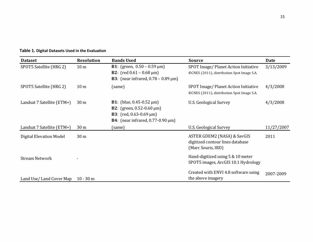
Dataset Resolution Bands Used Source Date
SPOT5 Satellite (HRG 2) 10 m B1: (green, 0.50 – 0.59 µm) SPOT Image/ Planet Action Initiative 3/13/2009
B2: (red 0.61 – 0.68 µm) ©CNES (2011), distribution Spot Image S.A.
B3: (near infrared, 0.78 – 0.89 µm)
SPOT5 Satellite (HRG 2) 10 m (same) SPOT Image/ Planet Action Initiative 4/3/2008
©CNES (2011), distribution Spot Image S.A.
Landsat 7 Satellite (ETM+) 30 m B1: (blue, 0.45-0.52 µm) U.S. Geological Survey 4/3/2008
B2: (green, 0.52-0.60 µm)
B3: (red, 0.63-0.69 µm)
B4: (near infrared, 0.77-0.90 µm)
Landsat 7 Satellite (ETM+) 30 m (same) U.S. Geological Survey 11/27/2007
Digital Elevation Model 30 m ASTER GDEM2 (NASA) & SavGIS
digitized contour lines database
(Marc Souris, IRD)
2011
Stream Network - Hand-digitized using 5 & 10 meter
SPOT5 images, ArcGIS 10.1 Hydrology
Land Use/ Land Cover Map 10 - 30 m
Created with ENVI 4.8 software using
the above imagery 2007-2009
Table 1. Digital Datasets Used in the Evaluation
16
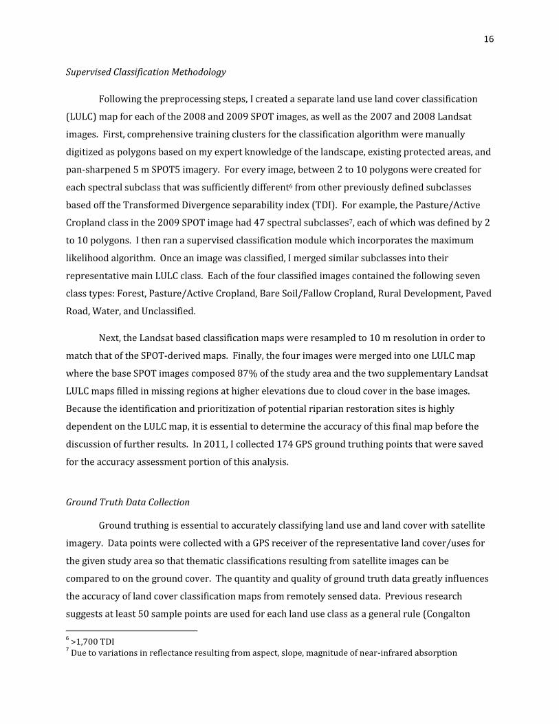
Supervised Classification Methodology
Following the preprocessing steps, I created a separate land use land cover classification
(LULC) map for each of the 2008 and 2009 SPOT images, as well as the 2007 and 2008 Landsat
images. First, comprehensive training clusters for the classification algorithm were manually
digitized as polygons based on my expert knowledge of the landscape, existing protected areas, and
pan-sharpened 5 m SPOT5 imagery. For every image, between 2 to 10 polygons were created for
each spectral subclass that was sufficiently different6 from other previously defined subclasses
based off the Transformed Divergence separability index (TDI). For example, the Pasture/Active
Cropland class in the 2009 SPOT image had 47 spectral subclasses7, each of which was defined by 2
to 10 polygons. I then ran a supervised classification module which incorporates the maximum
likelihood algorithm. Once an image was classified, I merged similar subclasses into their
representative main LULC class. Each of the four classified images contained the following seven
class types: Forest, Pasture/Active Cropland, Bare Soil/Fallow Cropland, Rural Development, Paved
Road, Water, and Unclassified.
Next, the Landsat based classification maps were resampled to 10 m resolution in order to
match that of the SPOT-derived maps. Finally, the four images were merged into one LULC map
where the base SPOT images composed 87% of the study area and the two supplementary Landsat
LULC maps filled in missing regions at higher elevations due to cloud cover in the base images.
Because the identification and prioritization of potential riparian restoration sites is highly
dependent on the LULC map, it is essential to determine the accuracy of this final map before the
discussion of further results. In 2011, I collected 174 GPS ground truthing points that were saved
for the accuracy assessment portion of this analysis.
Ground Truth Data Collection
Ground truthing is essential to accurately classifying land use and land cover with satellite
imagery. Data points were collected with a GPS receiver of the representative land cover/uses for
the given study area so that thematic classifications resulting from satellite images can be
compared to on the ground cover. The quantity and quality of ground truth data greatly influences
the accuracy of land cover classification maps from remotely sensed data. Previous research
suggests at least 50 sample points are used for each land use class as a general rule (Congalton
6 >1,700 TDI
7 Due to variations in reflectance resulting from aspect, slope, magnitude of near-infrared absorption
17
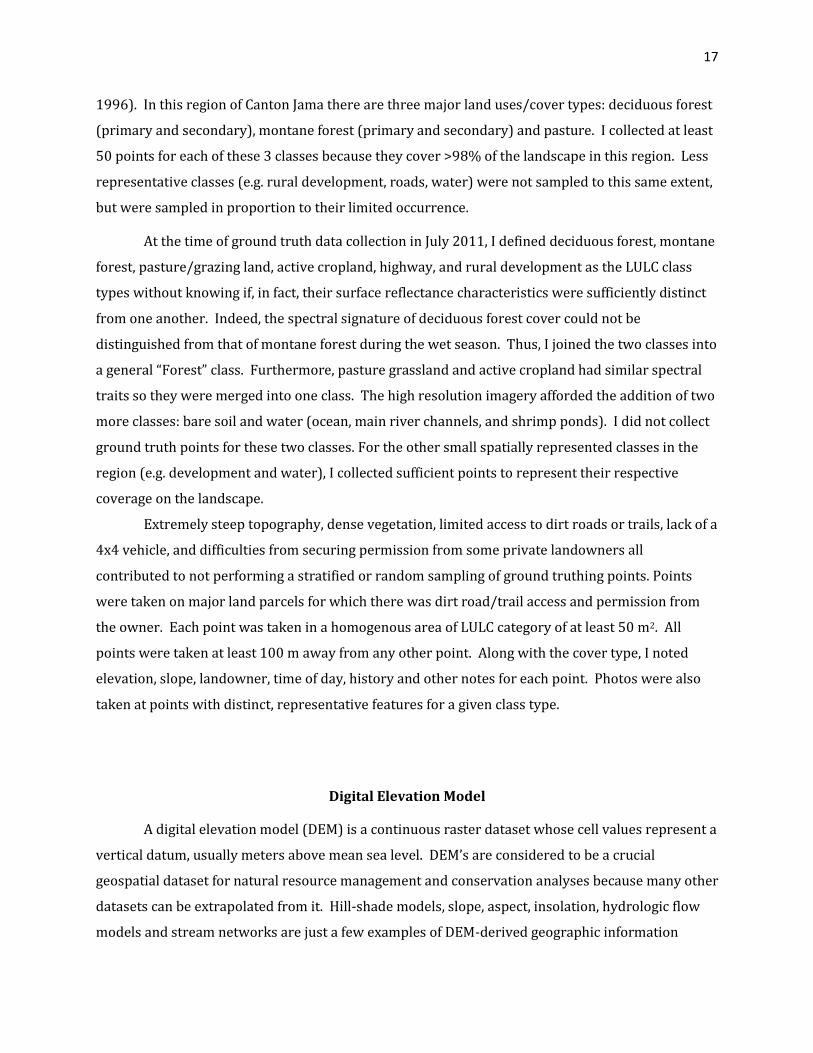
1996). In this region of Canton Jama there are three major land uses/cover types: deciduous forest
(primary and secondary), montane forest (primary and secondary) and pasture. I collected at least
50 points for each of these 3 classes because they cover >98% of the landscape in this region. Less
representative classes (e.g. rural development, roads, water) were not sampled to this same extent,
but were sampled in proportion to their limited occurrence.
At the time of ground truth data collection in July 2011, I defined deciduous forest, montane
forest, pasture/grazing land, active cropland, highway, and rural development as the LULC class
types without knowing if, in fact, their surface reflectance characteristics were sufficiently distinct
from one another. Indeed, the spectral signature of deciduous forest cover could not be
distinguished from that of montane forest during the wet season. Thus, I joined the two classes into
a general “Forest” class. Furthermore, pasture grassland and active cropland had similar spectral
traits so they were merged into one class. The high resolution imagery afforded the addition of two
more classes: bare soil and water (ocean, main river channels, and shrimp ponds). I did not collect
ground truth points for these two classes. For the other small spatially represented classes in the
region (e.g. development and water), I collected sufficient points to represent their respective
coverage on the landscape.
Extremely steep topography, dense vegetation, limited access to dirt roads or trails, lack of a
4x4 vehicle, and difficulties from securing permission from some private landowners all
contributed to not performing a stratified or random sampling of ground truthing points. Points
were taken on major land parcels for which there was dirt road/trail access and permission from
the owner. Each point was taken in a homogenous area of LULC category of at least 50 m2. All
points were taken at least 100 m away from any other point. Along with the cover type, I noted
elevation, slope, landowner, time of day, history and other notes for each point. Photos were also
taken at points with distinct, representative features for a given class type.
Digital Elevation Model
A digital elevation model (DEM) is a continuous raster dataset whose cell values represent a
vertical datum, usually meters above mean sea level. DEM’s are considered to be a crucial
geospatial dataset for natural resource management and conservation analyses because many other
datasets can be extrapolated from it. Hill-shade models, slope, aspect, insolation, hydrologic flow
models and stream networks are just a few examples of DEM-derived geographic information
18
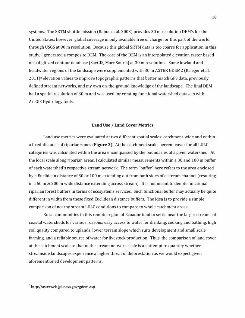
systems. The SRTM shuttle mission (Rabus et al. 2003) provides 30 m resolution DEM’s for the
United States; however, global coverage in only available free of charge for this part of the world
through USGS at 90 m resolution. Because this global SRTM data is too coarse for application in this
study, I generated a composite DEM. The core of the DEM is an interpolated elevation raster based
on a digitized contour database (SavGIS, Marc Souris) at 30 m resolution. Some lowland and
headwater regions of the landscape were supplemented with 30 m ASTER GDEM2 (Krieger et al.
2011)8 elevation values to improve topographic patterns that better match GPS data, previously
defined stream networks, and my own on-the-ground knowledge of the landscape. The final DEM
had a spatial resolution of 30 m and was used for creating functional watershed datasets with
ArcGIS Hydrology tools.
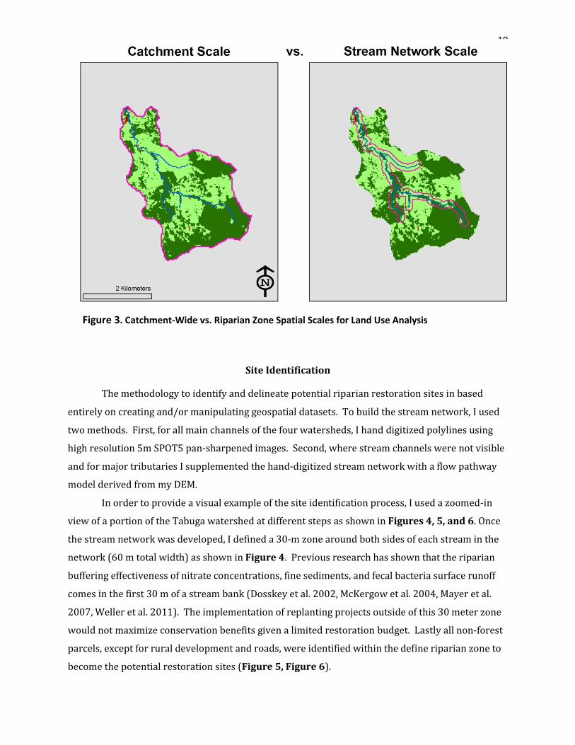
Land Use / Land Cover Metrics
Land use metrics were evaluated at two different spatial scales: catchment-wide and within
a fixed-distance of riparian zones (Figure 3). At the catchment scale, percent cover for all LULC
categories was calculated within the area encompassed by the boundaries of a given watershed. At
the local scale along riparian areas, I calculated similar measurements within a 30 and 100 m buffer
of each watershed’s respective stream network. The term “buffer” here refers to the area enclosed
by a Euclidean distance of 30 or 100 m extending out from both sides of a stream channel (resulting
in a 60 m & 200 m wide distance extending across stream). It is not meant to denote functional
riparian forest buffers in terms of ecosystems services. Such functional buffer may actually be quite
different in width from these fixed Euclidean distance buffers. The idea is to provide a simple
comparison of nearby stream LULC conditions to compare to whole catchment areas.
Rural communities in this remote region of Ecuador tend to settle near the larger streams of
coastal watersheds for various reasons: easy access to water for drinking, cooking and bathing, high
soil quality compared to uplands, lower terrain slope which suits development and small scale
farming, and a reliable source of water for livestock production. Thus, the comparison of land cover
at the catchment scale to that of the stream network scale is an attempt to quantify whether
streamside landscapes experience a higher threat of deforestation as we would expect given
aforementioned development patterns.
8 http://asterweb.jpl.nasa.gov/gdem.asp
19
Site Identification
The methodology to identify and delineate potential riparian restoration sites in based
entirely on creating and/or manipulating geospatial datasets. To build the stream network, I used
two methods. First, for all main channels of the four watersheds, I hand digitized polylines using
high resolution 5m SPOT5 pan-sharpened images. Second, where stream channels were not visible
and for major tributaries I supplemented the hand-digitized stream network with a flow pathway
model derived from my DEM.
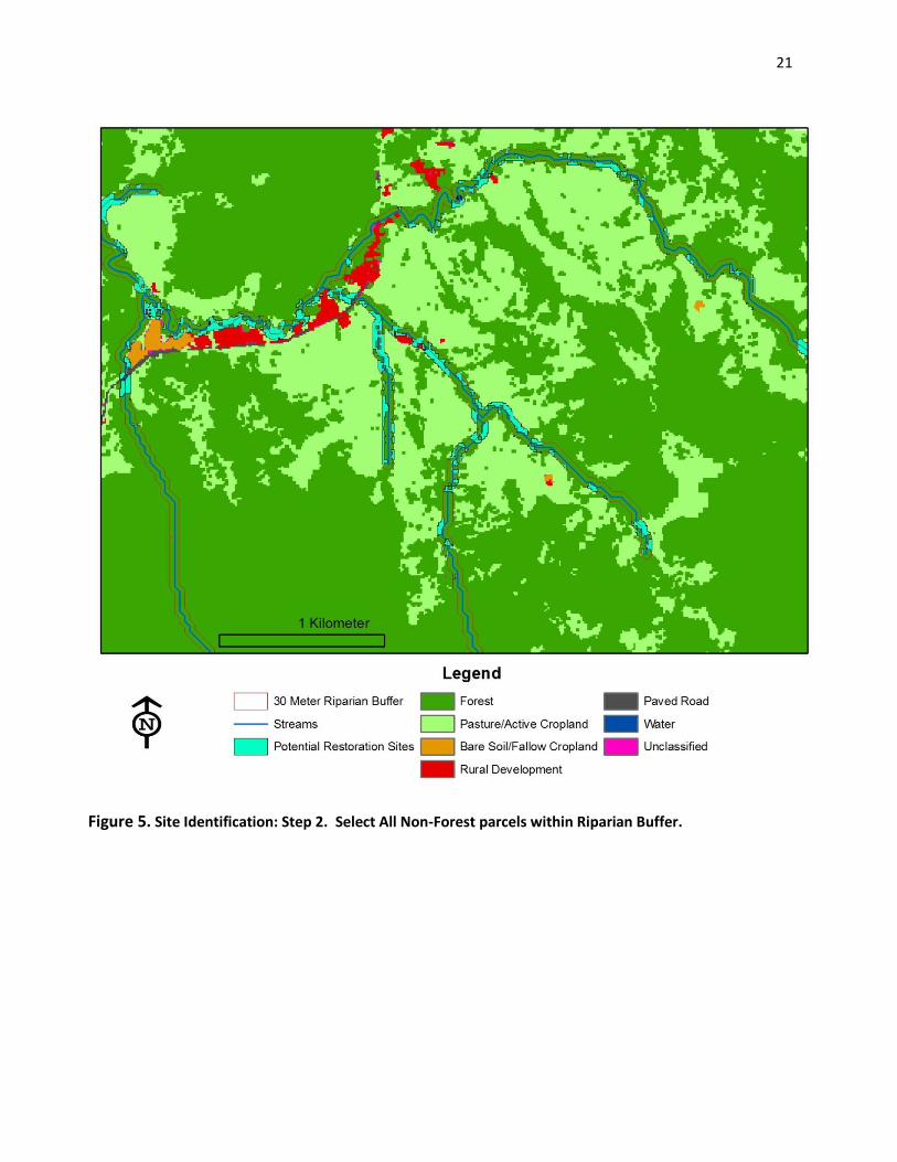
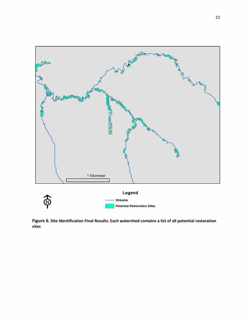
In order to provide a visual example of the site identification process, I used a zoomed-in
view of a portion of the Tabuga watershed at different steps as shown in Figures 4, 5, and 6. Once
the stream network was developed, I defined a 30-m zone around both sides of each stream in the
network (60 m total width) as shown in Figure 4. Previous research has shown that the riparian
buffering effectiveness of nitrate concentrations, fine sediments, and fecal bacteria surface runoff
comes in the first 30 m of a stream bank (Dosskey et al. 2002, McKergow et al. 2004, Mayer et al.
2007, Weller et al. 2011). The implementation of replanting projects outside of this 30 meter zone
would not maximize conservation benefits given a limited restoration budget. Lastly all non-forest
parcels, except for rural development and roads, were identified within the define riparian zone to
become the potential restoration sites (Figure 5, Figure 6).
Figure 3. Catchment-Wide vs. Riparian Zone Spatial Scales for Land Use Analysis

20
Figure 4. Site Identification: Step 1, Defining Riparian Zones (30-m buffer around both sides of streams)
21
Figure 5. Site Identification: Step 2. Select All Non-Forest parcels within Riparian Buffer.
22
Figure 6. Site Identification Final Results: Each watershed contains a list of all potential restoration sites
23
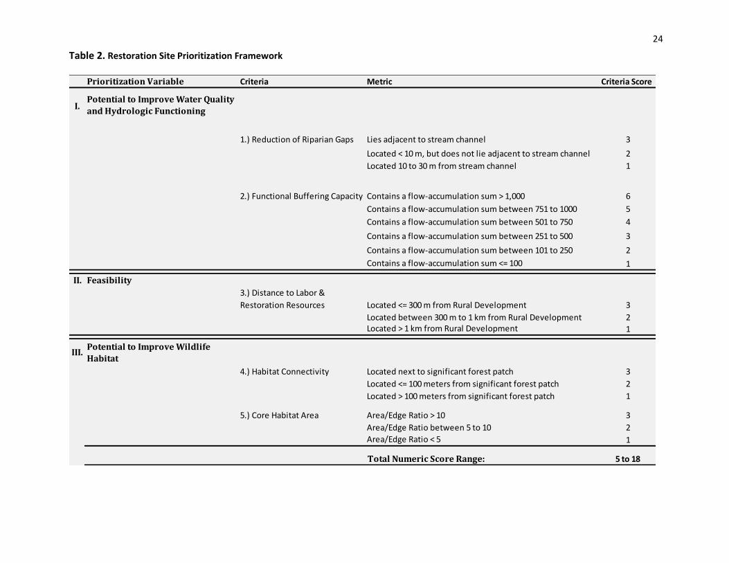
Site Prioritization
The prioritization framework utilized geospatial datasets developed from this project to
assign a prioritization category of “high”, “moderate, or “low” to each of the potential restoration
sites. It is based on a point ranking system that is adaptable and can be replicated for watershed
management planning outside of the study area. In order to match the restoration objectives, the
framework consists of three main variables: (1) potential to improve water quality and hydrologic
function, (b) feasibility, and (c) potential for wildlife habitat enhancement. Each of these variables
was composed of a set of criteria based on landscape metrics which assigned a score to each of the
restoration units. In all, there are 5 selection criteria (Table 2) whose point scores range from 1-3
or 1-6. Higher number scores correspond to higher restoration priority.
Potential to improve water quality and hydrologic function
Criteria 1: Reduction of Riparian Gaps (Score: 1-3)
This metric determines where riparian gaps occur along the stream network. That
is, where there is no forest cover between non-point sources of pollution and the stream
channel. For sites that lie directly next the stream channel, they are considered to be a
riparian gap and are given a score of “3” denoting high priority for restoration. Sites further
away from the stream channels which have a forest buffer between itself and the stream are
given lower scores and thus lower priority.
Criteria 2: Functional Buffering Capacity (Score: 1-6)
Surface flows in a catchment area do not drain evenly into riparian zones. They are
rather concentrated based off geomorphological traits where the majority of surface area
drains into a small percentage of the riparian zone (Dosskey et al. 2002, McGlynn and
Seibert 2003). This metric basically rates each potential site on its potential to act as a
functional buffer with a score of “1” being low potential and “6” being the highest potential.
Using a DEM-derived flow accumulation model, the amount of upslope terrain that
contributes to flow pathways can be calculated for each potential site. I gave this variable a
weight of 1-6 instead of 1-3 because this function is critical to serving the overall objectives
of reducing pollution runoff from nearby cattle pastures into waterways.
24
Prioritization Variable Criteria Metric Criteria Score
I.Potential to Improve Water Quality
and Hydrologic Functioning
1.) Reduction of Riparian Gaps Lies adjacent to stream channel 3
Located < 10 m, but does not lie adjacent to stream channel 2
Located 10 to 30 m from stream channel 1
2.) Functional Buffering Capacity Contains a flow-accumulation sum > 1,000 6
Contains a flow-accumulation sum between 751 to 1000 5
Contains a flow-accumulation sum between 501 to 750 4
Contains a flow-accumulation sum between 251 to 500 3
Contains a flow-accumulation sum between 101 to 250 2
Contains a flow-accumulation sum <= 100 1
II. Feasibility
3.) Distance to Labor &
Restoration Resources Located <= 300 m from Rural Development 3
Located between 300 m to 1 km from Rural Development 2Located > 1 km from Rural Development 1
III.Potential to Improve Wildlife
Habitat
4.) Habitat Connectivity Located next to significant forest patch 3
Located <= 100 meters from significant forest patch 2
Located > 100 meters from significant forest patch 1
5.) Core Habitat Area Area/Edge Ratio > 10 3
Area/Edge Ratio between 5 to 10 2
Area/Edge Ratio < 5 1
Total Numeric Score Range: 5 to 18
Table 2. Restoration Site Prioritization Framework
25
Feasibility
Criteria 3: Access to labor and restoration resources (Score: 1-3)
The remote nature of portions of these watersheds makes some potential sites less
feasible than others. The farther a site is from rural communities and roads, the more costly
it will be to carry out reforestation projects. Those sites closes to development were ranked
the highest priority (“3”) and those furthest away were ranked lowest (“1”).
Potential for wildlife habitat enhancement
Criteria 4: Habitat connectivity (Score: 1-3)
In order to encourage maximum forest cover connectivity, I ranked potential
restoration sites that lie adjacent to significant forest patches as having the highest priority
(score = “3”) over other sites that are located further from forests. Sites further away
received a score of “1” or “2” because reforestation may simply create an island forest that
does connect existing forest habitat.
Criteria 5: Core Habitat Area (Score: 1-3)
This metric calculated an area/edge ratio for each potential restoration area.
Habitat patches that maximize core area and limit edge length protect wildlife from the
ecological impacts from abundant edge effects such as introduction of invasive species and
micro climate warming at ecosystem boundaries. Potential sites with the highest area/edge
ratios received high priority scores (“3”) and those with lower ratios received lower scores
according to the metrics in Table 2.
26
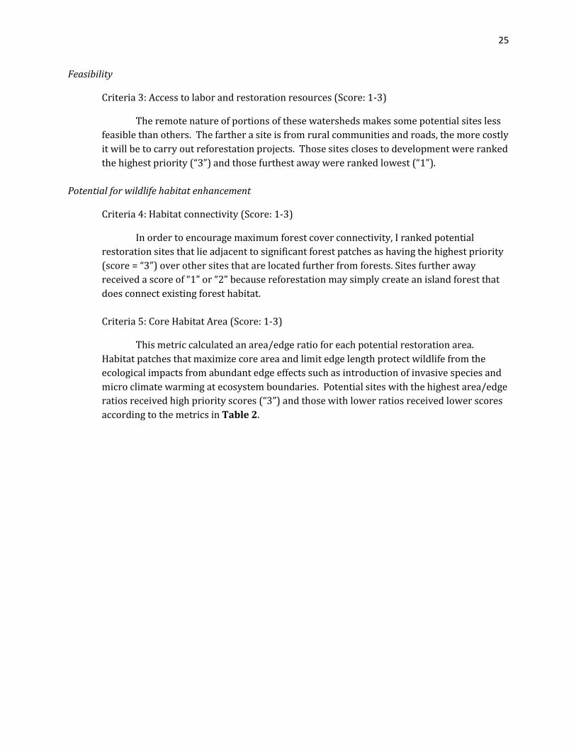
Figure 7. Prioritization Map: An Example from the Tabuga Watershed. Numbered sites in red have highest priority for restoration focus.
27
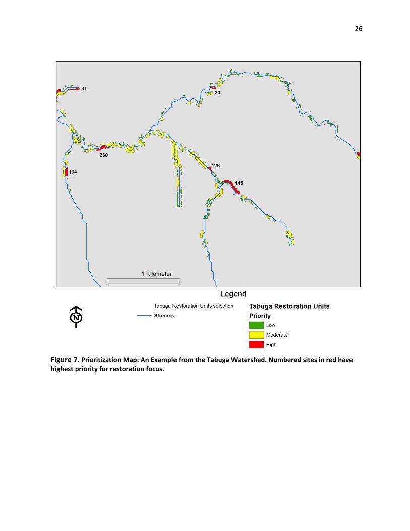
Final Prioritization Ranking
Once criteria scores were assessed, they were summed to yield a final prioritization score
with possible values ranging from 5-18. According to Table 3, restoration sites were then
categorized as “high”, “moderate”, or “low” based on a score range. An example of the application of
the prioritization model is shown in Figure 7. Similar to the zoomed-in examples in the previous
identification methods section, this figure depicts the prioritized restoration units which are color
coded to match their respective rating.
3. RESULTS
General Land Use, Land Cover Characteristics
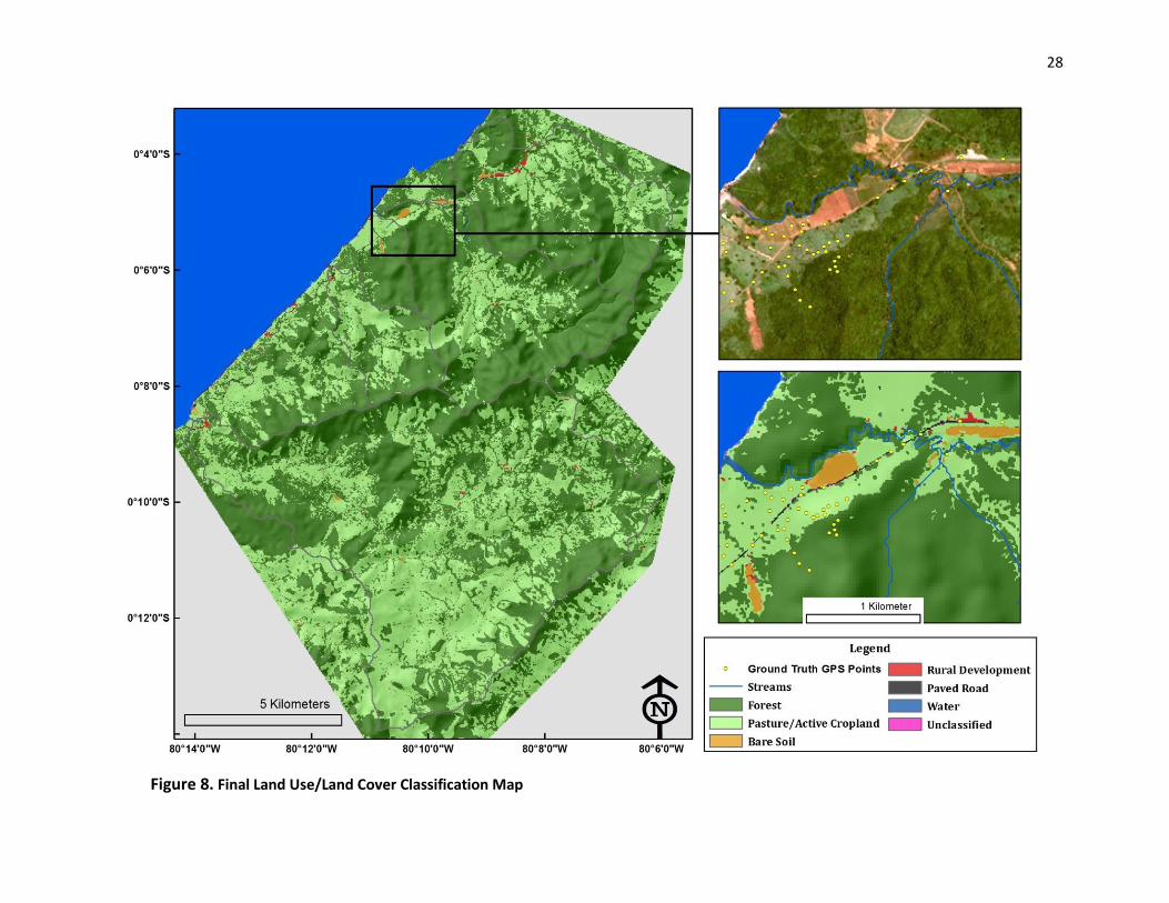
The land use land cover map easily depicts the nature of land use along the north coast of
Manabí Province (Figure 8). Depending on the watershed, between 98-99% of the land is
composed of either forest or grazing pasture. Roads, rural development and inactive cropland/bare
soil make up the remaining 1-2%. Across the study area, 58.7% of the landscape is covered in
forest (primary and secondary) and 40.8% is cattle pasture9. In general, all four watersheds in this
project area share a similar landscape characterization where lowland valleys and low-moderate
sloped hillsides are dominated by pasture and the upland, steeper sloped regions have a higher
proportion of semi-deciduous forest or montane forest. For all portions of the study area above an
elevation of 300 m, 76% is covered in forest. In the Camarones and Tasaste watersheds, forest
cover is over 90% at upper elevations. The final land use/ land cover categories are Forest,
Pasture/Active Cropland, Bare Soil/Fallow Cropland, Rural Development, Paved Roads, Water
Unclassified.
9 The pasture class actually includes pasture and active cropland. The % cover of cropland could not be quantified,
but is considered to be nominal.
Prioritization Rating: Score Range:
High 15 - 18
Moderate 10-14
Low 5-9
Table 3. Final Prioritization Rank System
28
Figure 8. Final Land Use/Land Cover Classification Map
29
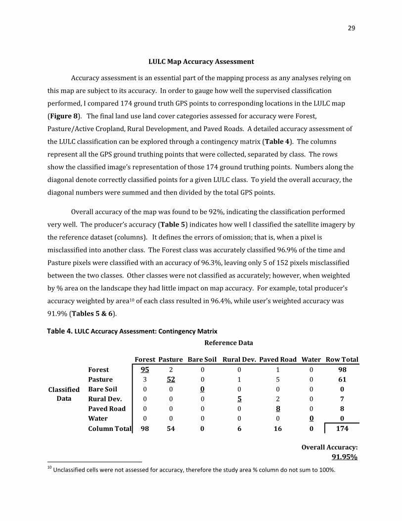
LULC Map Accuracy Assessment
Accuracy assessment is an essential part of the mapping process as any analyses relying on
this map are subject to its accuracy. In order to gauge how well the supervised classification
performed, I compared 174 ground truth GPS points to corresponding locations in the LULC map
(Figure 8). The final land use land cover categories assessed for accuracy were Forest,
Pasture/Active Cropland, Rural Development, and Paved Roads. A detailed accuracy assessment of
the LULC classification can be explored through a contingency matrix (Table 4). The columns
represent all the GPS ground truthing points that were collected, separated by class. The rows
show the classified image’s representation of those 174 ground truthing points. Numbers along the
diagonal denote correctly classified points for a given LULC class. To yield the overall accuracy, the
diagonal numbers were summed and then divided by the total GPS points.
Overall accuracy of the map was found to be 92%, indicating the classification performed
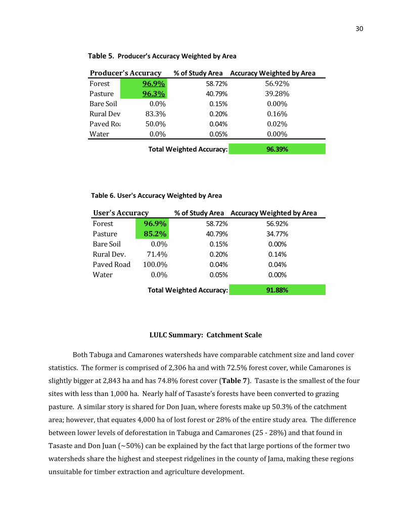
very well. The producer’s accuracy (Table 5) indicates how well I classified the satellite imagery by
the reference dataset (columns). It defines the errors of omission; that is, when a pixel is
misclassified into another class. The Forest class was accurately classified 96.9% of the time and
Pasture pixels were classified with an accuracy of 96.3%, leaving only 5 of 152 pixels misclassified
between the two classes. Other classes were not classified as accurately; however, when weighted
by % area on the landscape they had little impact on map accuracy. For example, total producer’s
accuracy weighted by area10 of each class resulted in 96.4%, while user’s weighted accuracy was
91.9% (Tables 5 & 6).
10
Unclassified cells were not assessed for accuracy, therefore the study area % column do not sum to 100%.
Forest Pasture Bare Soil Rural Dev. Paved Road Water Row Total
Forest 95 2 0 0 1 0 98
Pasture 3 52 0 1 5 0 61
Bare Soil 0 0 0 0 0 0 0
Rural Dev. 0 0 0 5 2 0 7
Paved Road 0 0 0 0 8 0 8
Water 0 0 0 0 0 0 0
Column Total: 98 54 0 6 16 0 174
91.95%
Classified
Data
Reference Data
Overall Accuracy:
Table 4. LULC Accuracy Assessment: Contingency Matrix
30
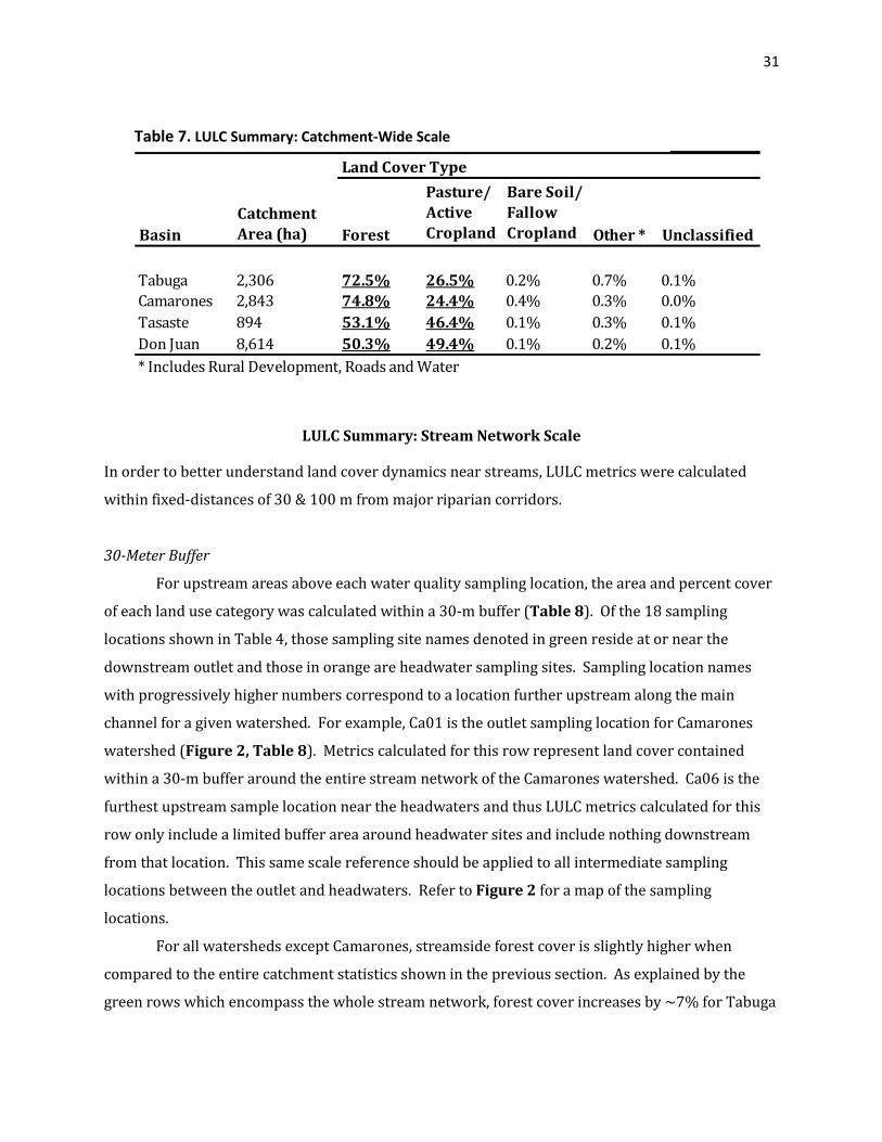
LULC Summary: Catchment Scale
Both Tabuga and Camarones watersheds have comparable catchment size and land cover
statistics. The former is comprised of 2,306 ha and with 72.5% forest cover, while Camarones is
slightly bigger at 2,843 ha and has 74.8% forest cover (Table 7). Tasaste is the smallest of the four
sites with less than 1,000 ha. Nearly half of Tasaste’s forests have been converted to grazing
pasture. A similar story is shared for Don Juan, where forests make up 50.3% of the catchment
area; however, that equates 4,000 ha of lost forest or 28% of the entire study area. The difference
between lower levels of deforestation in Tabuga and Camarones (25 - 28%) and that found in
Tasaste and Don Juan (~50%) can be explained by the fact that large portions of the former two
watersheds share the highest and steepest ridgelines in the county of Jama, making these regions
unsuitable for timber extraction and agriculture development.
% of Study Area Accuracy Weighted by Area
Forest 96.9% 58.72% 56.92%
Pasture 96.3% 40.79% 39.28%
Bare Soil 0.0% 0.15% 0.00%
Rural Dev. 83.3% 0.20% 0.16%
Paved Road 50.0% 0.04% 0.02%
Water 0.0% 0.05% 0.00%
96.39%
Producer's Accuracy
Total Weighted Accuracy:
Table 5. Producer’s Accuracy Weighted by Area
User's Accuracy % of Study Area Accuracy Weighted by Area
Forest 96.9% 58.72% 56.92%
Pasture 85.2% 40.79% 34.77%
Bare Soil 0.0% 0.15% 0.00%
Rural Dev. 71.4% 0.20% 0.14%
Paved Road 100.0% 0.04% 0.04%
Water 0.0% 0.05% 0.00%
91.88%Total Weighted Accuracy:
Table 6. User's Accuracy Weighted by Area
31
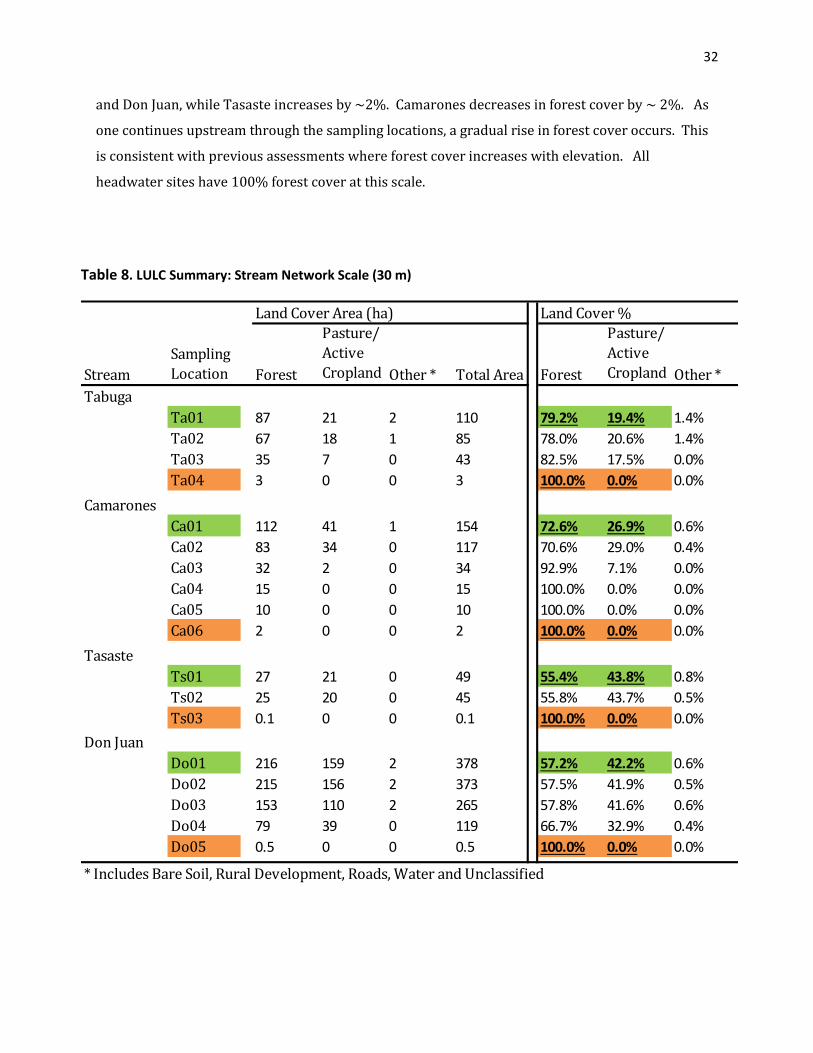
LULC Summary: Stream Network Scale
In order to better understand land cover dynamics near streams, LULC metrics were calculated
within fixed-distances of 30 & 100 m from major riparian corridors.
30-Meter Buffer
For upstream areas above each water quality sampling location, the area and percent cover
of each land use category was calculated within a 30-m buffer (Table 8). Of the 18 sampling
locations shown in Table 4, those sampling site names denoted in green reside at or near the
downstream outlet and those in orange are headwater sampling sites. Sampling location names
with progressively higher numbers correspond to a location further upstream along the main
channel for a given watershed. For example, Ca01 is the outlet sampling location for Camarones
watershed (Figure 2, Table 8). Metrics calculated for this row represent land cover contained
within a 30-m buffer around the entire stream network of the Camarones watershed. Ca06 is the
furthest upstream sample location near the headwaters and thus LULC metrics calculated for this
row only include a limited buffer area around headwater sites and include nothing downstream
from that location. This same scale reference should be applied to all intermediate sampling
locations between the outlet and headwaters. Refer to Figure 2 for a map of the sampling
locations.
For all watersheds except Camarones, streamside forest cover is slightly higher when
compared to the entire catchment statistics shown in the previous section. As explained by the
green rows which encompass the whole stream network, forest cover increases by ~7% for Tabuga
Forest
Pasture/
Active
Cropland
Bare Soil/
Fallow
Cropland Other * Unclassified
Tabuga 2,306 72.5% 26.5% 0.2% 0.7% 0.1%
Camarones 2,843 74.8% 24.4% 0.4% 0.3% 0.0%
Tasaste 894 53.1% 46.4% 0.1% 0.3% 0.1%
Don Juan 8,614 50.3% 49.4% 0.1% 0.2% 0.1%
Basin
Catchment
Area (ha)
* Includes Rural Development, Roads and Water
Land Cover Type
Table 7. LULC Summary: Catchment-Wide Scale
32
and Don Juan, while Tasaste increases by ~2%. Camarones decreases in forest cover by ~ 2%. As
one continues upstream through the sampling locations, a gradual rise in forest cover occurs. This
is consistent with previous assessments where forest cover increases with elevation. All
headwater sites have 100% forest cover at this scale.
Forest
Pasture/
Active
Cropland Other * Total Area Forest
Pasture/
Active
Cropland Other *
Tabuga
Ta01 87 21 2 110 79.2% 19.4% 1.4%
Ta02 67 18 1 85 78.0% 20.6% 1.4%
Ta03 35 7 0 43 82.5% 17.5% 0.0%
Ta04 3 0 0 3 100.0% 0.0% 0.0%
Camarones
Ca01 112 41 1 154 72.6% 26.9% 0.6%
Ca02 83 34 0 117 70.6% 29.0% 0.4%
Ca03 32 2 0 34 92.9% 7.1% 0.0%
Ca04 15 0 0 15 100.0% 0.0% 0.0%
Ca05 10 0 0 10 100.0% 0.0% 0.0%
Ca06 2 0 0 2 100.0% 0.0% 0.0%
Tasaste
Ts01 27 21 0 49 55.4% 43.8% 0.8%
Ts02 25 20 0 45 55.8% 43.7% 0.5%
Ts03 0.1 0 0 0.1 100.0% 0.0% 0.0%
Don Juan
Do01 216 159 2 378 57.2% 42.2% 0.6%
Do02 215 156 2 373 57.5% 41.9% 0.5%
Do03 153 110 2 265 57.8% 41.6% 0.6%
Do04 79 39 0 119 66.7% 32.9% 0.4%
Do05 0.5 0 0 0.5 100.0% 0.0% 0.0%
Stream
Sampling
Location
Land Cover Area (ha) Land Cover %
* Includes Bare Soil, Rural Development, Roads, Water and Unclassified
Table 8. LULC Summary: Stream Network Scale (30 m)
33
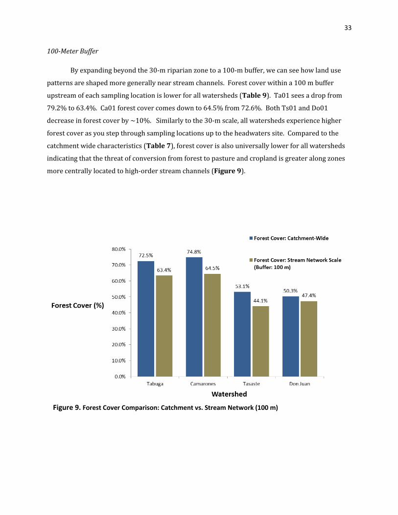
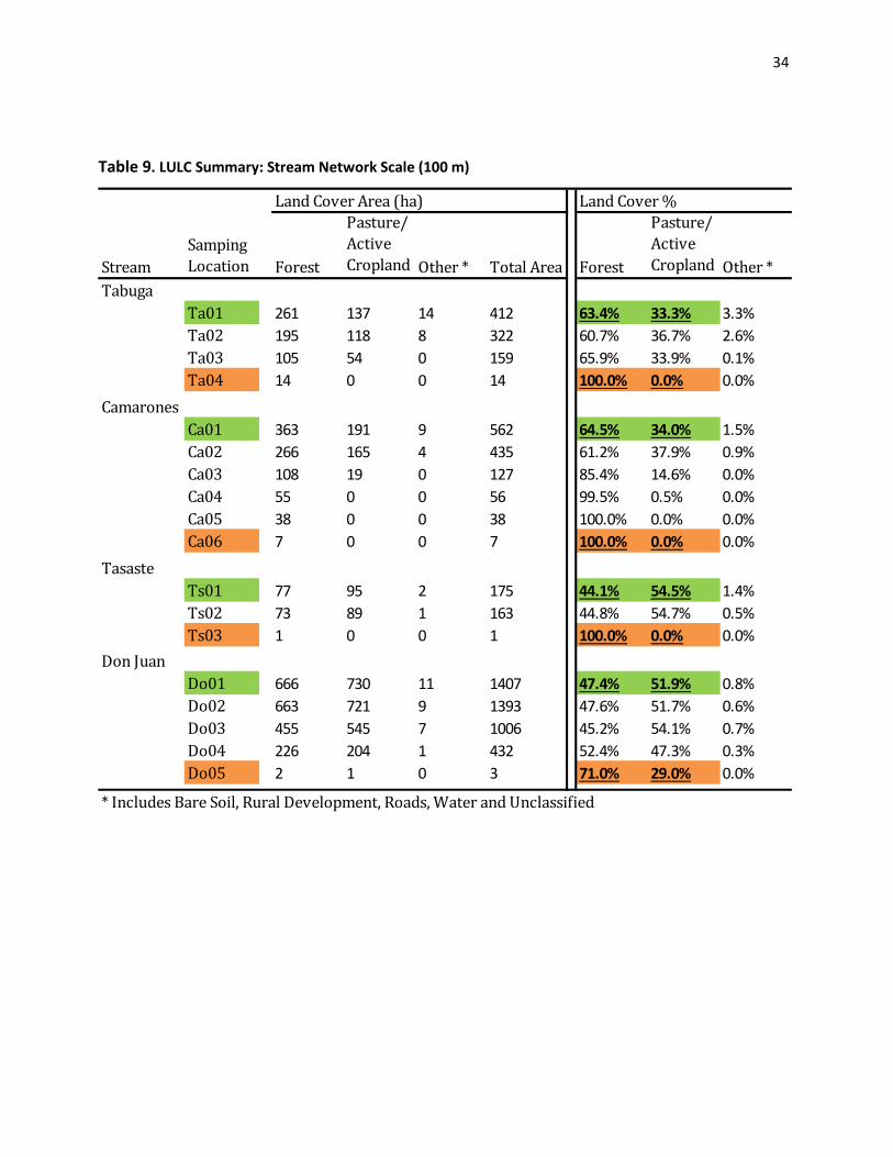
100-Meter Buffer
By expanding beyond the 30-m riparian zone to a 100-m buffer, we can see how land use
patterns are shaped more generally near stream channels. Forest cover within a 100 m buffer
upstream of each sampling location is lower for all watersheds (Table 9). Ta01 sees a drop from
79.2% to 63.4%. Ca01 forest cover comes down to 64.5% from 72.6%. Both Ts01 and Do01
decrease in forest cover by ~10%. Similarly to the 30-m scale, all watersheds experience higher
forest cover as you step through sampling locations up to the headwaters site. Compared to the
catchment wide characteristics (Table 7), forest cover is also universally lower for all watersheds
indicating that the threat of conversion from forest to pasture and cropland is greater along zones
more centrally located to high-order stream channels (Figure 9).
Figure 9. Forest Cover Comparison: Catchment vs. Stream Network (100 m)
34
Forest
Pasture/
Active
Cropland Other * Total Area Forest
Pasture/
Active
Cropland Other *
Tabuga
Ta01 261 137 14 412 63.4% 33.3% 3.3%
Ta02 195 118 8 322 60.7% 36.7% 2.6%
Ta03 105 54 0 159 65.9% 33.9% 0.1%
Ta04 14 0 0 14 100.0% 0.0% 0.0%
Camarones
Ca01 363 191 9 562 64.5% 34.0% 1.5%
Ca02 266 165 4 435 61.2% 37.9% 0.9%
Ca03 108 19 0 127 85.4% 14.6% 0.0%
Ca04 55 0 0 56 99.5% 0.5% 0.0%
Ca05 38 0 0 38 100.0% 0.0% 0.0%
Ca06 7 0 0 7 100.0% 0.0% 0.0%
Tasaste
Ts01 77 95 2 175 44.1% 54.5% 1.4%
Ts02 73 89 1 163 44.8% 54.7% 0.5%
Ts03 1 0 0 1 100.0% 0.0% 0.0%
Don Juan
Do01 666 730 11 1407 47.4% 51.9% 0.8%
Do02 663 721 9 1393 47.6% 51.7% 0.6%
Do03 455 545 7 1006 45.2% 54.1% 0.7%
Do04 226 204 1 432 52.4% 47.3% 0.3%
Do05 2 1 0 3 71.0% 29.0% 0.0%
Stream
Samping
Location
Land Cover Area (ha) Land Cover %
* Includes Bare Soil, Rural Development, Roads, Water and Unclassified
Table 9. LULC Summary: Stream Network Scale (100 m)
35
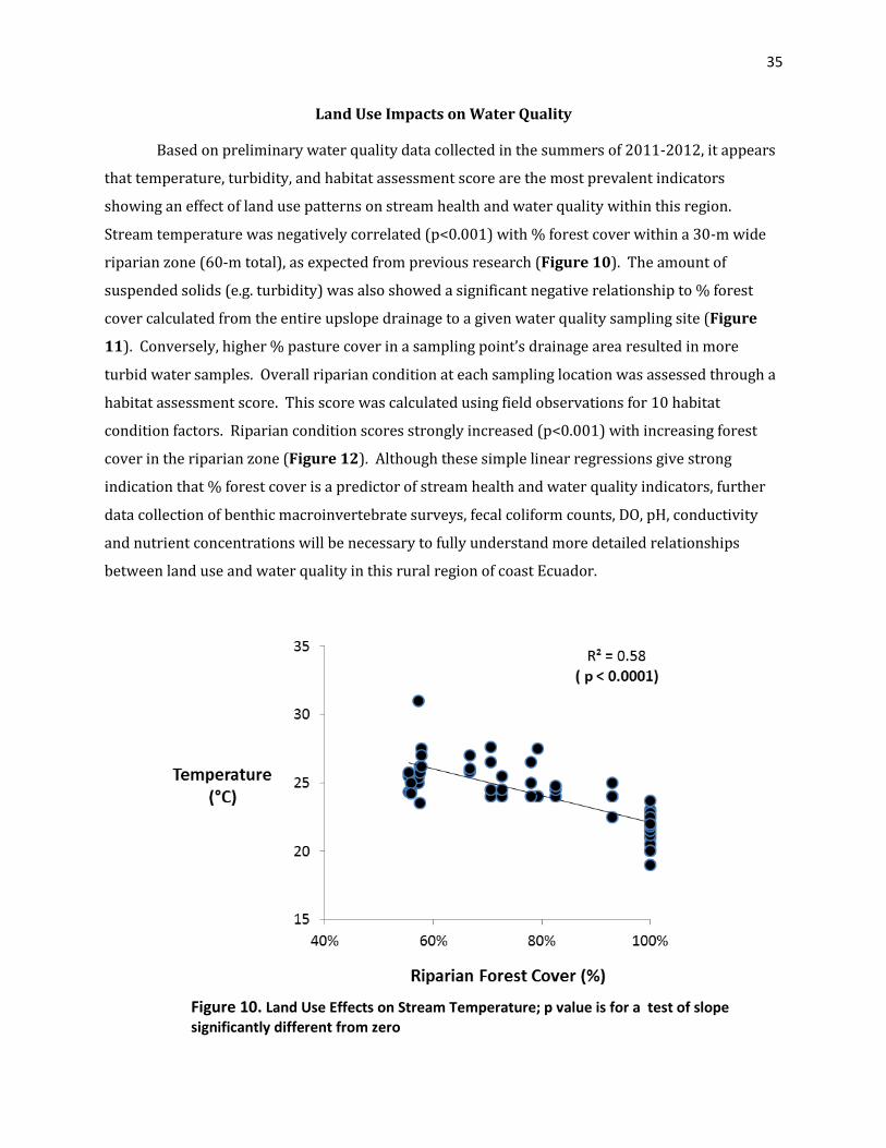
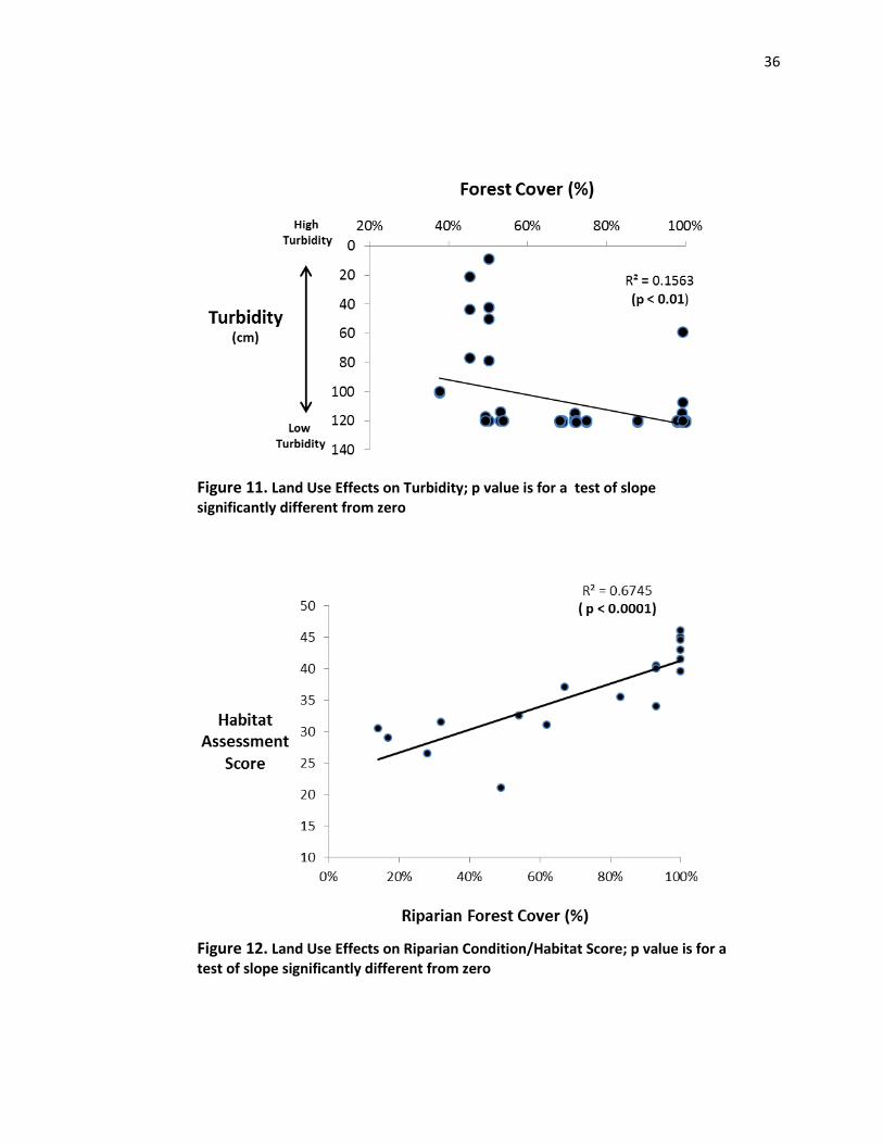
Land Use Impacts on Water Quality
Based on preliminary water quality data collected in the summers of 2011-2012, it appears
that temperature, turbidity, and habitat assessment score are the most prevalent indicators
showing an effect of land use patterns on stream health and water quality within this region.
Stream temperature was negatively correlated (p<0.001) with % forest cover within a 30-m wide
riparian zone (60-m total), as expected from previous research (Figure 10). The amount of
suspended solids (e.g. turbidity) was also showed a significant negative relationship to % forest
cover calculated from the entire upslope drainage to a given water quality sampling site (Figure
11). Conversely, higher % pasture cover in a sampling point’s drainage area resulted in more
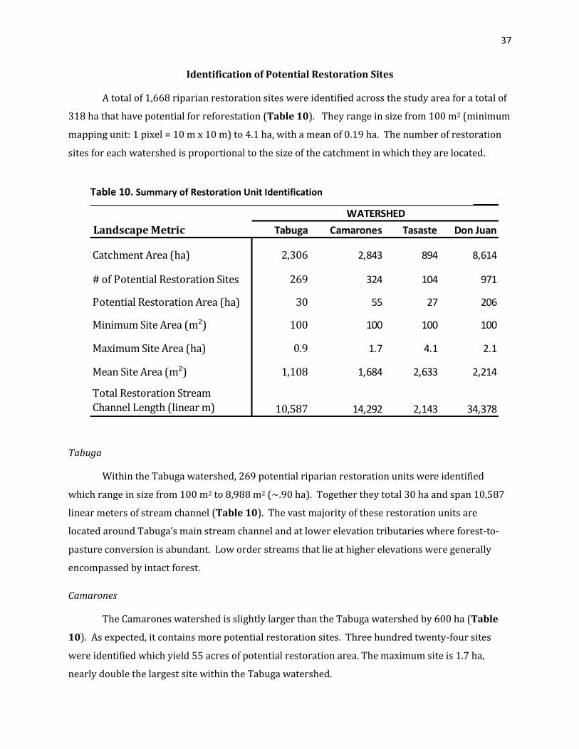
turbid water samples. Overall riparian condition at each sampling location was assessed through a
habitat assessment score. This score was calculated using field observations for 10 habitat
condition factors. Riparian condition scores strongly increased (p<0.001) with increasing forest
cover in the riparian zone (Figure 12). Although these simple linear regressions give strong
indication that % forest cover is a predictor of stream health and water quality indicators, further
data collection of benthic macroinvertebrate surveys, fecal coliform counts, DO, pH, conductivity
and nutrient concentrations will be necessary to fully understand more detailed relationships
between land use and water quality in this rural region of coast Ecuador.
Figure 10. Land Use Effects on Stream Temperature; p value is for a test of slope significantly different from zero
36
Figure 11. Land Use Effects on Turbidity; p value is for a test of slope significantly different from zero
Figure 12. Land Use Effects on Riparian Condition/Habitat Score; p value is for a test of slope significantly different from zero
37
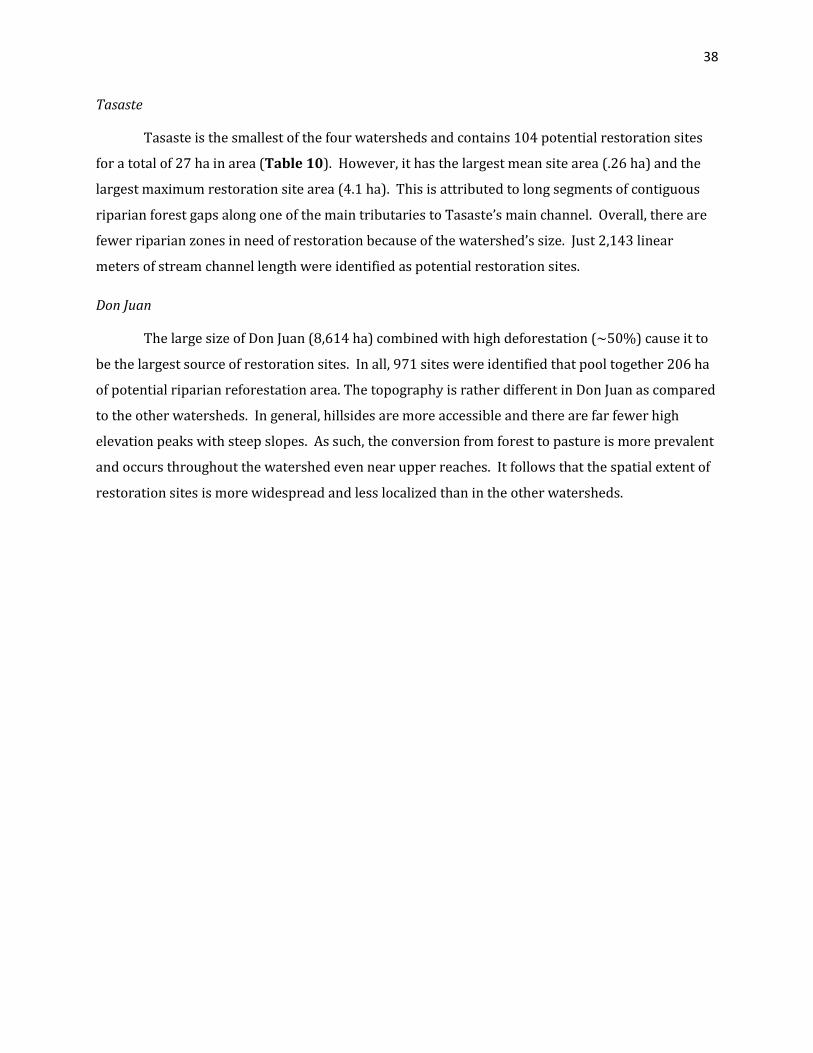
Identification of Potential Restoration Sites
A total of 1,668 riparian restoration sites were identified across the study area for a total of
318 ha that have potential for reforestation (Table 10). They range in size from 100 m2 (minimum
mapping unit: 1 pixel = 10 m x 10 m) to 4.1 ha, with a mean of 0.19 ha. The number of restoration
sites for each watershed is proportional to the size of the catchment in which they are located.
Tabuga
Within the Tabuga watershed, 269 potential riparian restoration units were identified
which range in size from 100 m2 to 8,988 m2 (~.90 ha). Together they total 30 ha and span 10,587
linear meters of stream channel (Table 10). The vast majority of these restoration units are
located around Tabuga’s main stream channel and at lower elevation tributaries where forest-to-
pasture conversion is abundant. Low order streams that lie at higher elevations were generally
encompassed by intact forest.
Camarones
The Camarones watershed is slightly larger than the Tabuga watershed by 600 ha (Table
10). As expected, it contains more potential restoration sites. Three hundred twenty-four sites
were identified which yield 55 acres of potential restoration area. The maximum site is 1.7 ha,
nearly double the largest site within the Tabuga watershed.
Landscape Metric Tabuga Camarones Tasaste Don Juan
Catchment Area (ha) 2,306 2,843 894 8,614
# of Potential Restoration Sites 269 324 104 971
Potential Restoration Area (ha) 30 55 27 206
Minimum Site Area (m²) 100 100 100 100
Maximum Site Area (ha) 0.9 1.7 4.1 2.1
Mean Site Area (m²) 1,108 1,684 2,633 2,214
Total Restoration Stream
Channel Length (linear m) 10,587 14,292 2,143 34,378
WATERSHED
Table 10. Summary of Restoration Unit Identification
38
Tasaste
Tasaste is the smallest of the four watersheds and contains 104 potential restoration sites
for a total of 27 ha in area (Table 10). However, it has the largest mean site area (.26 ha) and the
largest maximum restoration site area (4.1 ha). This is attributed to long segments of contiguous
riparian forest gaps along one of the main tributaries to Tasaste’s main channel. Overall, there are
fewer riparian zones in need of restoration because of the watershed’s size. Just 2,143 linear
meters of stream channel length were identified as potential restoration sites.
Don Juan
The large size of Don Juan (8,614 ha) combined with high deforestation (~50%) cause it to
be the largest source of restoration sites. In all, 971 sites were identified that pool together 206 ha
of potential riparian reforestation area. The topography is rather different in Don Juan as compared
to the other watersheds. In general, hillsides are more accessible and there are far fewer high
elevation peaks with steep slopes. As such, the conversion from forest to pasture is more prevalent
and occurs throughout the watershed even near upper reaches. It follows that the spatial extent of
restoration sites is more widespread and less localized than in the other watersheds.
39
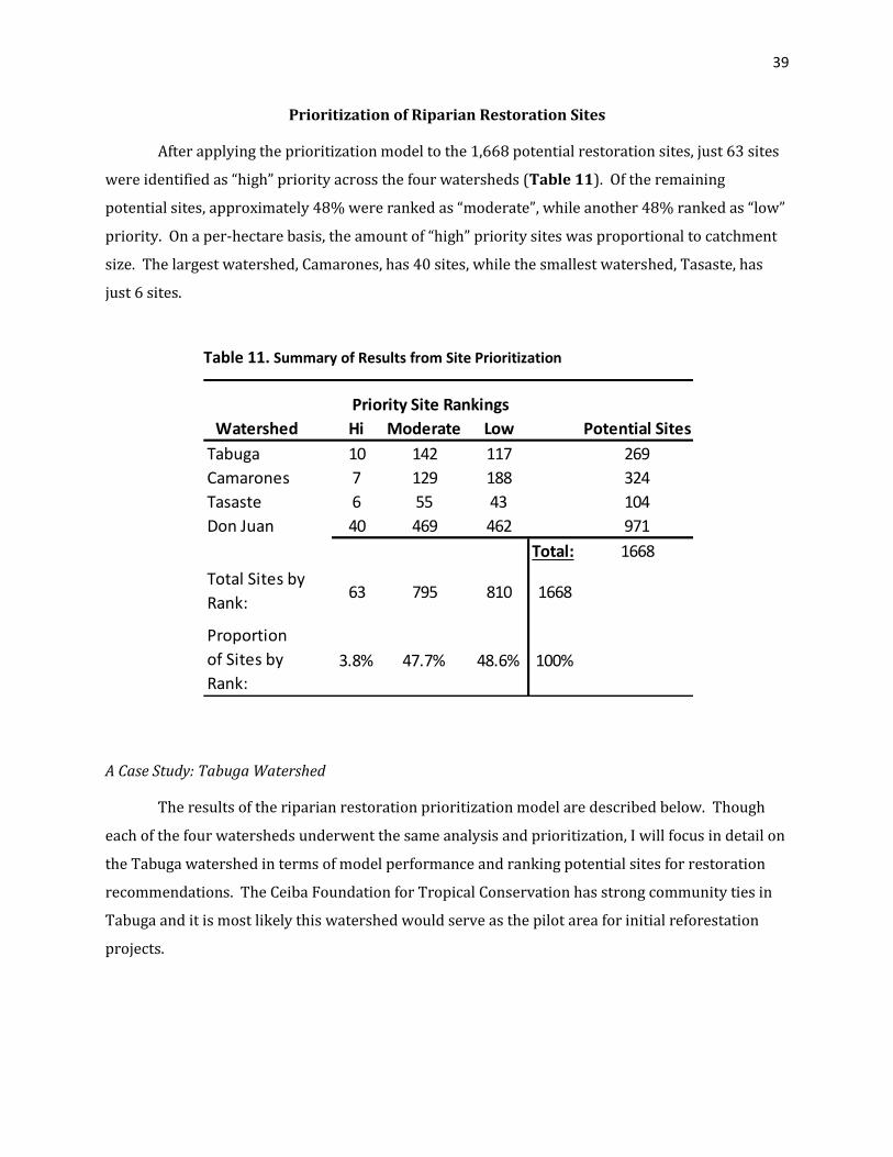
Prioritization of Riparian Restoration Sites
After applying the prioritization model to the 1,668 potential restoration sites, just 63 sites
were identified as “high” priority across the four watersheds (Table 11). Of the remaining
potential sites, approximately 48% were ranked as “moderate”, while another 48% ranked as “low”
priority. On a per-hectare basis, the amount of “high” priority sites was proportional to catchment
size. The largest watershed, Camarones, has 40 sites, while the smallest watershed, Tasaste, has
just 6 sites.
A Case Study: Tabuga Watershed
The results of the riparian restoration prioritization model are described below. Though
each of the four watersheds underwent the same analysis and prioritization, I will focus in detail on
the Tabuga watershed in terms of model performance and ranking potential sites for restoration
recommendations. The Ceiba Foundation for Tropical Conservation has strong community ties in
Tabuga and it is most likely this watershed would serve as the pilot area for initial reforestation
projects.
Watershed Hi Moderate Low Potential Sites
Tabuga 10 142 117 269
Camarones 7 129 188 324
Tasaste 6 55 43 104
Don Juan 40 469 462 971
Total: 1668
Total Sites by
Rank:63 795 810 1668
Proportion
of Sites by
Rank:
3.8% 47.7% 48.6% 100%
Priority Site Rankings
Table 11. Summary of Results from Site Prioritization
40
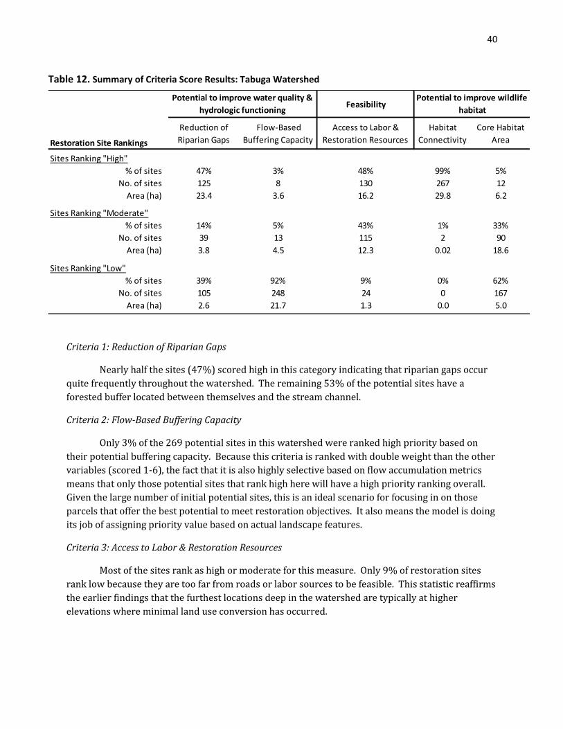
Criteria 1: Reduction of Riparian Gaps
Nearly half the sites (47%) scored high in this category indicating that riparian gaps occur
quite frequently throughout the watershed. The remaining 53% of the potential sites have a
forested buffer located between themselves and the stream channel.
Criteria 2: Flow-Based Buffering Capacity
Only 3% of the 269 potential sites in this watershed were ranked high priority based on
their potential buffering capacity. Because this criteria is ranked with double weight than the other
variables (scored 1-6), the fact that it is also highly selective based on flow accumulation metrics
means that only those potential sites that rank high here will have a high priority ranking overall.
Given the large number of initial potential sites, this is an ideal scenario for focusing in on those
parcels that offer the best potential to meet restoration objectives. It also means the model is doing
its job of assigning priority value based on actual landscape features.
Criteria 3: Access to Labor & Restoration Resources
Most of the sites rank as high or moderate for this measure. Only 9% of restoration sites
rank low because they are too far from roads or labor sources to be feasible. This statistic reaffirms
the earlier findings that the furthest locations deep in the watershed are typically at higher
elevations where minimal land use conversion has occurred.
Feasibility
Restoration Site Rankings
Reduction of
Riparian Gaps
Flow-Based
Buffering Capacity
Access to Labor &
Restoration Resources
Habitat
Connectivity
Core Habitat
Area
Sites Ranking "High"
% of sites 47% 3% 48% 99% 5%
No. of sites 125 8 130 267 12
Area (ha) 23.4 3.6 16.2 29.8 6.2
Sites Ranking "Moderate"
% of sites 14% 5% 43% 1% 33%
No. of sites 39 13 115 2 90
Area (ha) 3.8 4.5 12.3 0.02 18.6
Sites Ranking "Low"
% of sites 39% 92% 9% 0% 62%
No. of sites 105 248 24 0 167
Area (ha) 2.6 21.7 1.3 0.0 5.0
Potential to improve wildlife
habitat
Potential to improve water quality &
hydrologic functioning
Table 12. Summary of Criteria Score Results: Tabuga Watershed
41
Criteria 4: Habitat Connectivity
This measure was the least selective in assigning high priority rankings. Nearly all (99%) of
the potential sites received a high priority score. Future modification of this model will examine
landscape analyses in relation to forest connectivity that will help discern between sites that offer
the best ecological services from linking forest patches of differing size and location to other land
uses.
Criteria 5: Core Habitat Area
The majority of Tabuga’s restoration sites score low for this measure based on their core
area/edge ratio. Because many sites are small and composed of a single pixel (100 m2), this
measure helped the model focus on areas of significant size that were more realistic for
reforestation efforts and provided core area value for potential wildlife habitat improvement. Only
5% of the sites had a large enough area/edge ratio to be ranked as high priority. Criteria 2 and 5
are the most selective in determining overall top priority sites for the Tabuga watershed. Similar
results occurred for the other three watersheds in the study.
42
4. DISCUSSION
Interpretation of Results
The analysis of land cover change has shown that within the four coastal watersheds in the
study area, the severity of deforestation ranges from 24% to 50% primarily due to conversion to
pasture for livestock production. This type of land use change further increases by as much as 10%
for areas closest to higher order streams showing an increased threat to riparian zones. Keeping in
mind that loss of native forest cover throughout the vast majority of the coastal plain reaches a
staggering 80%-98%, it becomes clear that the preservation of these last forest fragments is critical
to the overall conservation goals in western Ecuador. The severity of deforestation at the
catchment-wide scale gives an early indication of overall watershed degradation and the potential
for reduced ecological functioning. However, catchment-wide summary metrics only measure
proportions of LULC and provide no insight into location of land use conversion. Determining land
use patterns within buffers of streams offers an approach to examine how land is managed within
the more accessible locations.
Inside riparian zones of 30 m surrounding streams (60 m total width), forest cover
increased nominally across all watersheds (except for Camarones which slightly decreased) when
compared to the catchment measurement (Tables 7 & 8). It appears there is a minor preference
for preserving a functional riparian buffer that is consistent with best management practices. As
the literature suggests, most riparian effectiveness occurs within the first 30 m of the stream
channel (Mayer et al. 2007). In general, forest cover along these narrow riparian areas is more or
less consistent with general forest cover in the catchment. Unfortunately, for watersheds with the
highest levels of deforestation (Tasaste and Don Juan), even an increase of 7% of forested riparian
area may offer little protection from a landscape that has lost half of its forest cover. At the very
least, riparian areas do not experience more forest loss when compared to the catchment scale.
The health of a given segment of stream is not entirely indicative of land cover within a
narrow 30 m zone. Upslope geomorphology and land use play critical roles in the transport of
nutrients, sources of organic matter, bacteria, fine sediments, and pollutants to stream networks.
By examining metrics within a 100-m riparian zone, the picture becomes clearer as to how land use
is characterized in broader areas adjacent to streams. All watersheds experience distinct drops in
forest cover between catchment-wide and the 100-meter buffer scale as shown in Figure 9.
Using preliminary water quality data from 18 sampling locations across the study area,
significant relationships were found between forest cover and the most standard stream health
indicators. Stream temperature, turbidity and habitat assessment (riparian health assessment)
43
proved to be the simplest and best indicators for detecting the effects of land use change on stream
water quality in this part western Ecuador. Stream temperature showed a significant negative
correlation with increasing % forest cover within a 30-m riparian buffer zone (60-m total width).
This empirically supports the notion that intact riparian canopy provides shade and moderates
potential solar radiation heating of water temperature. Turbidity, a measurement of suspended
particles in water and regarded as the simplest visual indicator of drinking water quality, increased
at sampling locations with higher proportions of cattle pasture within their drainage area. Lastly,
an in depth habitat assessment yielded riparian condition scores that were strongly and positively
correlated with increased forest cover in the proximate riparian zone11. Such findings were
expected and match results from similar assessments as carried out in the eastern Amazon of Brazil
(Figueiredo et al. 2010).
As mentioned previously, Canton Jama has the majority of the highest peaks along the
coastal mountain range in western Ecuador. Thus, it is not surprising to find the last few remnants
of semi-deciduous dry forest and coastal montane forest here. Fortunately, conservation NGO’s like
the Ceiba Foundation for Tropical Conservation (CFTC), Fundación Jatun Sacha, Third Millennium
Alliance, and Conservation International have all contributed to establishing protected reserves.
Several of these have proved to be important partners for the Ecuadorian government by helping
enroll landowners in the Socio Bosque payment for ecosystem services program over the past three
years. Moving forward, these key stakeholders will provide a crucial role in the expanded
protection of these special forests through the implementation of reforestation projects aimed at
connecting forest patches via riparian corridors. As CFTC continues to work in Canton Jama
studying relations between land use, water quality and human health, there is promise that future
watershed management goals will benefit both the well-being of remaining forest fragments and
the local communities that rely on freshwater resources. This project has taken the first step in
identifying and prioritizing the most suitable sites for riparian habitat restoration at the watershed
scale.
Among the 1,668 potential restoration sites identified within the study area, only 3.8%
scored in the highest priority class. These top ranked sites for reforestation consideration are
larger in size, maximize core area for wildlife habitat, and have the best potential to enhance
riparian buffer functioning once restored. Alternatively, the lowest ranked sites were smaller in
11
Defined by 30 meter distance out from each side of the stream bank and then 100 meters upstream of a sampling location
44
size, had low core area in relation to the sites’ perimeter, and less ability to provide buffer
functioning because they contained little or no upslope surface flow pathways. Based on the
prioritization methodology, this was expected for two reasons. First, the identification procedure
identified all non-forest parcels12 within a total 60-m buffer from the stream channel as potential
restoration sites. However, this allowed for parcels comprised of a single cell (10 x 10 m) to be
considered a potential site. Sites of this small size scored low for the area/edge ratio criteria and
would not be sufficiently large to enhance wildlife habitat.
Secondly, not all streamside riparian areas have the ability to buffer surface runoff. Upslope
geomorphology determines which areas receive abundant, moderate, or minimal surface flow. For
example, a study in New Zealand found that within a 280-ha watershed, 85% of surface runoff
entered streams through only 28% of the riparian zone (McGlynn and Seibert 2003). As mentioned
in section 3, I added increased weight to the functional buffering capacity scoring metric13 to
account for this highly selective landscape feature. Given a limited restoration budget, the main
goal with restoration planning on a large scale is to focus on riparian zones that will maximize
ecological services. This project’s objectives focus principally on the improvement of drinking
water quality by mitigating surface flow containing fine sediment and fecal bacteria from adjacent
grazing pastures. It would not be consistent with goals or be cost-effective to plant native trees
along a streamside zone that receives minimal upslope surface flow from non-point sources of
pollution.
Use and Limitations of Watershed Restoration Planning
This study uses the best available geospatial data to begin the restoration planning process
that would be otherwise impossible through in-depth field studies due to lack of time, human
resources and finances. The methodology employed here is the most cost-effective and repeatable
method for prioritizing potential restorable land parcels. The prioritization model has been applied
to four different watersheds showing its applicability and flexibility across different catchment
boundaries. Should further data become available, the model is also adaptable to incorporate new
information. Similar GIS-based restoration planning projects in Mexico and South America
developed ranking schemes that contained socioeconomic and cultural datasets specific to a given
focus area in addition to ecology based datasets (Gonzalez-Espinosa et al. 2007, Orsi and Geneletti
12
Excludes rural development and roads, which are considered to be permanent land uses. 13
Ranked 1-6 instead of 1-3.
45
2010, Orsi et al. 2011). Such information could augment the restoration planning within Canton
Jama.
There are certain limitations that arise when solely relying on existing geospatial data for
planning restoration projects. Certainly, the addition of further high quality datasets would
enhance the model robustness. For example, a large portion of the stream network used in this
project was generated with a 30-m resolution digital elevation model. In terms of flow pathways,
this resolution is fairly coarse and fails to account for the micro-topography that exists in all
landscapes. This loss of complexity generalizes surface flow patterns and may not fully describe
potential runoff impacts into streams. As new remote sensing technologies become operational,
these uncertainties will be addressed. In particular to DEMs, the TanDEM-X mission will soon offer
higher quality global elevation datasets with spatial resolution of 12 m and vertical error of 2 m
starting in 2014 (Lopez-Dekker et al. 2011). In the meantime, on the ground verification of the
results from my prioritization model will provide insight into the effectiveness of the composite
DEM14 that was used for identifying riparian zones containing high flow accumulation.
Another source of error comes from the accuracy of the LULC map which served as one of
the base datasets for the restoration planning model. Based on the initial assessment showing a
weighted producer’s accuracy of 96%, the classification performed very well. However, it should be
noted that the whole study area does not likely have this level of accuracy when considering
current ground cover. There is a two to four year gap between the satellite image acquisition dates
and ground control data collection in 2011. This amount of time is sufficient for minor land use
change. Such change would likely represent loss of forest cover as opposed to regeneration of
secondary forests. Also, there may not be a clear distinction between forest and pasture in areas
where pasture is beginning regeneration of secondary forest. The ground truthing points were
accurately identified within large, homogeneous land cover parcels while those near edges
experienced higher misclassification. Because riparian areas contain complex and fragmented
forest/pasture/cropland borders, there might be more inherent error in classifying these regions of
the landscape.
A more vigorous accuracy measurement based on a comprehensive and random sampling
across Canton Jama would strengthen the classification accuracy assessment. Yet, unrestricted
access to private lands and a substantial investment of time and money would be necessary for this
type of data collection. At this point in time, it is rather outside the scope of local stakeholder’s
14
SavGIS & ASTER GDEM2 (NASA)

46
resources. Clearly, using satellite imagery of 10-m resolution, this supervised classification has
resulted in a robust and validated LULC map based on the best available ground truthing reference
datasets.
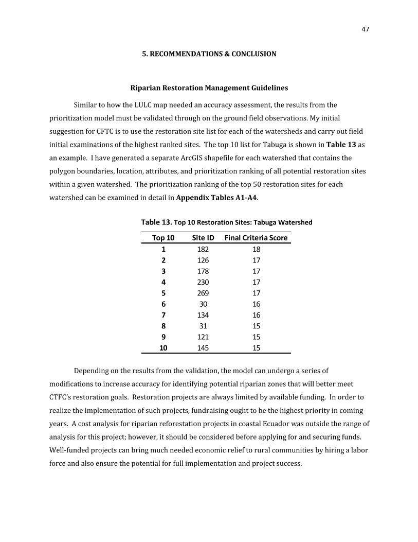
47
5. RECOMMENDATIONS & CONCLUSION
Riparian Restoration Management Guidelines
Similar to how the LULC map needed an accuracy assessment, the results from the
prioritization model must be validated through on the ground field observations. My initial
suggestion for CFTC is to use the restoration site list for each of the watersheds and carry out field
initial examinations of the highest ranked sites. The top 10 list for Tabuga is shown in Table 13 as
an example. I have generated a separate ArcGIS shapefile for each watershed that contains the
polygon boundaries, location, attributes, and prioritization ranking of all potential restoration sites
within a given watershed. The prioritization ranking of the top 50 restoration sites for each
watershed can be examined in detail in Appendix Tables A1-A4.
Depending on the results from the validation, the model can undergo a series of
modifications to increase accuracy for identifying potential riparian zones that will better meet
CTFC’s restoration goals. Restoration projects are always limited by available funding. In order to
realize the implementation of such projects, fundraising ought to be the highest priority in coming
years. A cost analysis for riparian reforestation projects in coastal Ecuador was outside the range of
analysis for this project; however, it should be considered before applying for and securing funds.
Well-funded projects can bring much needed economic relief to rural communities by hiring a labor
force and also ensure the potential for full implementation and project success.
Top 10 Site ID Final Criteria Score
1 182 18
2 126 17
3 178 17
4 230 17
5 269 17
6 30 16
7 134 16
8 31 15
9 121 15
10 145 15
Table 13. Top 10 Restoration Sites: Tabuga Watershed
48
Water Quality Data Collection
This section outlines recommendations for future water quality data collection with the
assumption that sufficient human and financial resources are available to carry out this level of
work. If possible, sampling consistently at least once a month, year-round would go a long way in
providing a continuous and reliable water quality dataset. This is important in the short run to
assess how current land use patterns relate to stream health and drinking water quality, but will
also be pertinent in the future for post-restoration monitoring. It would be even more ideal to
sample twice a month. Any sampling instruments should be calibrated frequently to ensure proper
measurements over time. Also, certain indicators such as temperature and dissolved oxygen
respond to daily oscillations, therefore data collection should occur at consistent times of day to
ensure validity of comparisons across sites or over time.
In regards to water quality and human health, the protocol could be augmented to sample
for indicators most directly related to drinking water quality. An initial effort has been made to
collect fecal coliform bacteria data; however, rigorous and repeated sampling will be needed
because coliform counts vary drastically over space and short periods of time. Additional
indicators of consideration include pH, conductivity, nutrient concentrations, presence of heavy
metals, and turbidity measured in NTU units. The combination of information from this type of
sampling and human health surveys/interviews taken in local communities will further shed light
on water quality and human health linkages.
The analysis of water quantity in these watersheds has yet to be explored. If possible, the
measurements of discharge following rain events and during wet season base flow may provide
insight as to how deforestation may be impacting the availability of water draining from the
watershed.
Additional GIS Data Collection
Geospatial datasets taken with a GPS receiver are considered to serve as reference datasets
with the least amount of locational error. The accuracy of the stream network could be greatly
enhanced by delineating the main channels and major tributaries on foot with a GPS device. Since
cropland areas were hard to distinguish from pasture land, new and large active cropland should be
traversed and added to a GIS dataset. It would also serve the project well to determine land
49
ownership information on parcels considered to be of high priority for restoration. It is highly
likely that landowners may not want to reforest riparian areas that are under current production
and generating income. Lastly, anytime there is potential to collect additional LULC ground truth
points it would benefit the confidence of the accuracy assessment.
Conclusion
In summary, I have created a new suite of digital geographic datasets that are significant to
this region of high conservation value including the following: land use/land cover map (10 m
resolution) and ground-truthing dataset, a cloud-free composite satellite image (2 images from
SPOT5, 2 from Landsat ETM+), a hand-digitized stream network based on high resolution SPOT5
images (5 m) and a hydrologic flow accumulation model, a digital elevation model, watershed and
sub-catchment boundaries, and a geospatial toolkit that incorporates the above databases to
effectively locate riparian corridors that are in greatest need of reforestation.
Although the watersheds of Tabuga, Camarones, Tasaste and Don Juan have not lost as
much forest cover in comparison to the majority of coastal Ecuador, evidence from this study
suggests that forest to pasture conversion of 24% to 50% negatively impacts riparian condition and
water quality sufficiently to warrant the need for habitat restoration projects. Using the best
available geospatial data, this evaluation has identified and prioritized a total of 63 riparian
restoration units across the four watersheds15. These sites represent the most likely candidates for
meeting the restoration objectives of improving water quality and providing wildlife habitat
connectivity. The prioritization model proved highly effective and adaptable across different
watersheds. The fact that it selected only 3.8% of the 1,668 potential sites as highest priority shows
that restoration planning through remote sensing and geospatial modeling is the quickest and most
affordable method for determining where to begin restoration efforts across a 14,000+ ha
landscape.
15
Tabuga: 10, Camarones: 7, Tasaste: 6, and Don Juan: 40
50
7. REFERENCES
Allan, J. D. 2004. Landscapes and Riverscapes: The Influence of Land Use on Stream Ecosystems. Annual Review of Ecology, Evolution, and Systematics 35:257-284.
Baker, M. E., D. E. Weller, and T. E. Jordan. 2006. Improved methods for quantifying potential nutrient interception by riparian buffers. Landscape Ecology 21:1327-1345.
Barton, D. R., W. D. Taylor, and R. M. Biette. 1985. DIMENSIONS OF RIPARIAN BUFFER STRIPS REQUIRED TO MAINTAIN TROUT HABITAT IN SOUTHERN ONTARIO CANADA STREAMS. North American Journal of Fisheries Management 5:364-378.
Bojsen, B. H. and D. Jacobsen. 2003. Effects of deforestation on macroinvertebrate diversity and assemblage structure in Ecuadorian Amazon streams. Archiv Fur Hydrobiologie 158:317-342.
Bourque, C. P. A. and J. H. Pomeroy. 2001. Effects of forest harvesting on summer stream temperatures in New Brunswick, Canada: an inter-catchment, multiple-year comparison. Hydrology and Earth System Sciences 5:599-613.
Burkhead, N. M. and H. L. Jelks. 2001. Effects of suspended sediment on the reproductive success of the tricolor shiner, a crevice-spawning minnow. Transactions of the American Fisheries Society 130:959-968.
Buss, D. F., D. F. Baptista, J. L. Nessimian, and M. Egler. 2004. Substrate specificity, environmental degradation and disturbance structuring macroinvertebrate assemblages in neotropical streams. Hydrobiologia 518:179-188.
Chuvieco, E. and A. Huete. 2009. Fundamentals of satellite remote sensing. CRC Press Inc. Congalton, R. G. 1996. Accuracy assessment: a critical component of land cover mapping. Gap analysis: a
landscape approach to biodiversity planning:119-131. de Koning, F., M. Aguiñaga, M. Bravo, M. Chiu, M. Lascano, T. Lozada, and L. Suarez. 2011. Bridging the
gap between forest conservation and poverty alleviation: the Ecuadorian Socio Bosque program. Environmental Science & Policy 14:531-542.
Diario, E. 2009. Informan sobre proyecto de forestacion para al rio, Chone, Manabi. El Diario. Dodson, C. H. and A. H. Gentry. 1991. Biological Extinction in Western Ecuador. Annals of the Missouri
Botanical Garden 78:273-295. Dosskey, M. G., M. J. Helmers, D. E. Eisenhauer, T. G. Franti, and K. D. Hoagland. 2002. Assessment of
concenrated flow through riparian buffers. Journal of Soil and Water Conservation 57:336-343. Economist, T. 2003. The Americas: Cut down; Logging in Ecuador. Pages 60-36 The Economist. The
Economist Intelligence Unit, London, United States, London. Ehrman, T. P. and G. A. Lamberti. 1992. HYDRAULIC AND PARTICULATE MATTER RETENTION IN A 3RD-
ORDER INDIANA STREAM. Journal of the North American Benthological Society 11:341-349. Fenoglio, S., G. Badino, and F. Bona. 2002. Benthic macroinvertebrate communities as indicators of river
environment quality: an experience in Nicaragua. Revista De Biologia Tropical 50:1125-1131. Figueiredo, R. O., D. Markewitz, E. A. Davidson, A. E. Schuler, O. dos S. Watrin, and P. de Souza Silva.
2010. Land-use effects on the chemical attributes of low-order streams in the eastern Amazon. Journal of Geophysical Research 115.
Figueroa, R., C. Valdovinos, E. Araya, and O. Parra. 2003. Benthic macroinvertebrates as indicators of water quality of southern Chile rivers. Revista Chilena De Historia Natural 76:275-285.
Findlay, S., J. M. Quinn, C. W. Hickey, G. Burrell, and M. Downes. 2001. Effects of land use and riparian flowpath on delivery of dissolved organic carbon to streams. Limnology and Oceanography 46:345-355.
51
George, I., A. Anzil, and P. Servais. 2004. Quantification of fecal coliform inputs to aquatic systems through soil leaching. Water Research 38:611-618.
Gonzalez-Espinosa, M., N. Ramirez-Marcial, A. C. Newton, J. M. Rey-Benayas, A. Camacho-Cruz, J. J. Armesto, A. Lara, A. C. Premoli, G. Williams-Linera, A. Altamirano, C. Alvarez-Aquino, M. Cortes, C. Echeverria, L. Galindo-Jaimes, M. A. Muniz-Castro, M. C. Nunez-Avila, R. A. Pedraza, A. E. Rovere, C. Smith-Ramirez, O. Thiers, and C. Zamorano. 2007. Restoration of Forest Ecosystems in Fragmented Landscapes of Temperate and Montane Tropical Latin America.
Gregory, S. V., F. J. Swanson, W. A. McKee, and K. W. Cummins. 1991. AN ECOSYSTEM PERSPECTIVE OF RIPARIAN ZONES. Bioscience 41:540-551.
Guerrero, M. 2010. En la provincial de Manabi se incrementan deslizamientos de tierra. El Nuevo Impresario.
Gurnell, A. M., K. J. Gregory, and G. E. Petts. 1995. THE ROLE OF COARSE WOODY DEBRIS IN FOREST AQUATIC HABITATS - IMPLICATIONS FOR MANAGEMENT. Aquatic Conservation-Marine and Freshwater Ecosystems 5:143-166.
Johnson, L. B., D. H. Breneman, and C. Richards. 2003. Macroinvertebrate community structure and function associated with large wood in low gradient streams. River Research and Applications 19:199-218.
Krieger, T., W. Curtis, and J. Haase. 2011. Global Validation of the ASTER Global Digital Elevation Model (GDEM) Version 2. . Report to the ASTER GDEM Version 2 Validation Team.
Lopez-Dekker, P., P. Prats, F. De Zan, D. Schulze, G. Krieger, and A. Moreira. 2011. TanDEM-X First DEM Acquisition: A Crossing Orbit Experiment. Ieee Geoscience and Remote Sensing Letters 8:943-947.
López, S., R. Sierra, and M. Tirado. 2010. Tropical Deforestation in the Ecuadorian Chocó: Logging Practices and Socio-spatial Relationships. The Geographical Bulletin 51:3-22.
Lorion, C. M. and B. P. Kennedy. 2009. Relationships between deforestation, riparian forest buffers and benthic macroinvertebrates in neotropical headwater streams. Freshwater Biology 54:165-180.
Lowrance, R., R. Todd, J. Fail, O. Hendrickson, R. Leonard, and L. Asmussen. 1984. RIPARIAN FORESTS AS NUTRIENT FILTERS IN AGRICULTURAL WATERSHEDS. Bioscience 34:374-377.
Maridet, L., J. G. Wasson, M. Philippe, and C. Amoros. 1995. BENTHIC ORGANIC-MATTER DYNAMICS IN 3 STREAMS - RIPARIAN VEGETATION OR BED MORPHOLOGY CONTROL. Archiv Fur Hydrobiologie 132:415-425.
Martin, T. L., N. K. Kaushik, J. T. Trevors, and H. R. Whiteley. 1999. Review: Denitrification in temperate climate riparian zones. Water Air and Soil Pollution 111:171-186.
Mayer, P. M., S. K. Reynolds, Jr., M. D. McCutchen, and T. J. Canfield. 2007. Meta-analysis of nitrogen removal in riparian buffers. Journal of Environmental Quality 36:1172-1180.
McGlynn, B. L. and J. Seibert. 2003. Distributed assessment of contributing area and riparian buffering along stream networks. Water Resources Research 39.
McKergow, L. A., I. P. Prosser, R. B. Grayson, and D. Heiner. 2004. Performance of grass and rainforest riparian buffers in the wet tropics, Far North Queensland. 2. Water quality. Australian Journal of Soil Research 42:485-498.
Miserendino, M. L., R. Casaux, M. Archangelsky, C. Y. Di Prinzio, C. Brand, and A. M. Kutschker. 2011. Assessing land-use effects on water quality, in-stream habitat, riparian ecosystems and biodiversity in Patagonian northwest streams. Sci Total Environ 409:612-624.
Myers, N. 1988. Threatened biotas: "hot spots" in tropical forests. The Environmentalist 8:187-208. Myers, N., R. A. Mittermeier, C. G. Mittermeier, A. B. d. F. Gustavo, and J. Kent. 2000. Biodiversity
hotspots for conservation priorities. Nature 403:853-858. Neill, D. 1999. Vegetation. Vegetation Types. Catalogue of Vascular Plants of Ecuador:13-25.
52
Orsi, F., R. L. Church, and D. Geneletti. 2011. Restoring forest landscapes for biodiversity conservation and rural livelihoods: A spatial optimisation model. Environmental Modelling & Software 26:1622-1638.
Orsi, F. and D. Geneletti. 2010. Identifying priority areas for Forest Landscape Restoration in Chiapas (Mexico): An operational approach combining ecological and socioeconomic criteria. Landscape and Urban Planning 94:20-30.
Osborne, L. L. and D. A. Kovacic. 1993. RIPARIAN VEGETATED BUFFER STRIPS IN WATER-QUALITY RESTORATION AND STREAM MANAGEMENT. Freshwater Biology 29:243-258.
Quinn, J. M. 2000. Effects of pastoral development. Rabus, B., M. Eineder, A. Roth, and R. Bamler. 2003. The shuttle radar topography mission - a new class
of digital elevation models acquired by spaceborne radar. Isprs Journal of Photogrammetry and Remote Sensing 57:241-262.
Sanchez, R. 2006. Cobertura Vegetal de la Republica del Ecuador, empleando informacion satelital. CLIRSEN, Quito, Ecuador.
Sierra, R. 1999. Propuesta preliminar de un sistema de clasificación de vegetación para el Ecuador continental. Proyecto INEFAN-GEF-BIRF y EcoCiencia.
Sierra, R. and J. Stallings. 1998. The dynamics and social organization of tropical deforestation in Northwest Ecuador, 1983-1995. Human Ecology 26:135-161.
Soldner, M., I. Stephen, L. Ramos, R. Angus, N. C. Wells, A. Grosso, and M. Crane. 2004. Relationship between macroinvertebrate fauna and environmental variables in small streams of the Dominican Republic. Water Research 38:863-874.
Southgate, D. and M. Whitaker. 1992. PROMOTING RESOURCE DEGRADATION IN LATIN-AMERICA - TROPICAL DEFORESTATION, SOIL-EROSION, AND COASTAL ECOSYSTEM DISTURBANCE IN ECUADOR. Economic Development and Cultural Change 40:787-807.
Stauffer, J. C., R. M. Goldstein, and R. M. Newman. 2000. Relationship of wooded riparian zones and runoff potential to fish community composition in agricultural streams. Canadian Journal of Fisheries and Aquatic Sciences 57:307-316.
Sutherland, A. B., J. L. Meyer, and E. P. Gardiner. 2002. Effects of land cover on sediment regime and fish assemblage structure in four southern Appalachian streams. Freshwater Biology 47:1791-1805.
Swanson, F. J., T. K. Kratz, N. Caine, and R. G. Woodmansee. 1988. LANDFORM EFFECTS ON ECOSYSTEM PATTERNS AND PROCESSES. Bioscience 38:92-98.
Uriarte, M., C. B. Yackulic, Y. Lim, and J. A. Arce-Nazario. 2011. Influence of land use on water quality in a tropical landscape: a multi-scale analysis. Landscape Ecology 26:1151-1164.
Vieira, N., S. J. Bates, O. D. Solberg, K. Ponce, R. Howsmon, W. Cevallos, G. Trueba, L. Riley, and J. N. S. Eisenberg. 2007. High prevalence of enteroinvasive Escherichia coli isolated in a remote region of northern coastal Ecuador. American Journal of Tropical Medicine and Hygiene 76:528-533.
Walser, C. A. and H. L. Bart. 1999. Influence of agriculture on in-stream habitat and fish community structure in Piedmont watersheds of the Chattahoochee River System. Ecology of Freshwater Fish 8:237-246.
Wang, L. Z., J. Lyons, P. Kanehl, and R. Gatti. 1997. Influences of watershed land use on habitat quality and biotic integrity in Wisconsin streams. Fisheries 22:6-12.
WAV. 2011. Water Action Volunteers website. http://watermonitoring.uwex.edu/wav/. Weller, D. E., M. E. Baker, and T. E. Jordan. 2011. Effects of riparian buffers on nitrate concentrations in
watershed discharges: new models and management implications. Ecological Applications 21:1679-1695.
Wood, P. J. and P. D. Armitage. 1997. Biological effects of fine sediment in the lotic environment. Environmental Management 21:203-217.

53
Woodward, C. and J. Meisl. 2010. Ceiba Foundation for Tropical Conservation Year in Review. Kapok Newsletter 6:1-2.
Wunder, S. 2001. The economics of deforestation; the example of Ecuador. Page n/a Scitech Book News. Book News, Inc., Portland, United States, Portland.
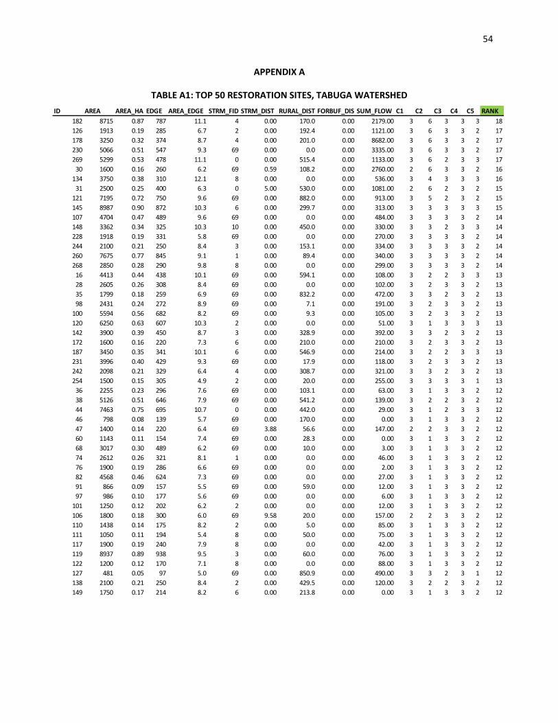
54
APPENDIX A
TABLE A1: TOP 50 RESTORATION SITES, TABUGA WATERSHED
ID AREA AREA_HA EDGE AREA_EDGE STRM_FID STRM_DIST RURAL_DIST FORBUF_DIS SUM_FLOW C1 C2 C3 C4 C5 RANK
182 8715 0.87 787 11.1 4 0.00 170.0 0.00 2179.00 3 6 3 3 3 18
126 1913 0.19 285 6.7 2 0.00 192.4 0.00 1121.00 3 6 3 3 2 17
178 3250 0.32 374 8.7 4 0.00 201.0 0.00 8682.00 3 6 3 3 2 17
230 5066 0.51 547 9.3 69 0.00 0.0 0.00 3335.00 3 6 3 3 2 17
269 5299 0.53 478 11.1 0 0.00 515.4 0.00 1133.00 3 6 2 3 3 17
30 1600 0.16 260 6.2 69 0.59 108.2 0.00 2760.00 2 6 3 3 2 16
134 3750 0.38 310 12.1 8 0.00 0.0 0.00 536.00 3 4 3 3 3 16
31 2500 0.25 400 6.3 0 5.00 530.0 0.00 1081.00 2 6 2 3 2 15
121 7195 0.72 750 9.6 69 0.00 882.0 0.00 913.00 3 5 2 3 2 15
145 8987 0.90 872 10.3 6 0.00 299.7 0.00 313.00 3 3 3 3 3 15
107 4704 0.47 489 9.6 69 0.00 0.0 0.00 484.00 3 3 3 3 2 14
148 3362 0.34 325 10.3 10 0.00 450.0 0.00 330.00 3 3 2 3 3 14
228 1918 0.19 331 5.8 69 0.00 0.0 0.00 270.00 3 3 3 3 2 14
244 2100 0.21 250 8.4 3 0.00 153.1 0.00 334.00 3 3 3 3 2 14
260 7675 0.77 845 9.1 1 0.00 89.4 0.00 340.00 3 3 3 3 2 14
268 2850 0.28 290 9.8 8 0.00 0.0 0.00 299.00 3 3 3 3 2 14
16 4413 0.44 438 10.1 69 0.00 594.1 0.00 108.00 3 2 2 3 3 13
28 2605 0.26 308 8.4 69 0.00 0.0 0.00 102.00 3 2 3 3 2 13
35 1799 0.18 259 6.9 69 0.00 832.2 0.00 472.00 3 3 2 3 2 13
98 2431 0.24 272 8.9 69 0.00 7.1 0.00 191.00 3 2 3 3 2 13
100 5594 0.56 682 8.2 69 0.00 9.3 0.00 105.00 3 2 3 3 2 13
120 6250 0.63 607 10.3 2 0.00 0.0 0.00 51.00 3 1 3 3 3 13
142 3900 0.39 450 8.7 3 0.00 328.9 0.00 392.00 3 3 2 3 2 13
172 1600 0.16 220 7.3 6 0.00 210.0 0.00 210.00 3 2 3 3 2 13
187 3450 0.35 341 10.1 6 0.00 546.9 0.00 214.00 3 2 2 3 3 13
231 3996 0.40 429 9.3 69 0.00 17.9 0.00 118.00 3 2 3 3 2 13
242 2098 0.21 329 6.4 4 0.00 308.7 0.00 321.00 3 3 2 3 2 13
254 1500 0.15 305 4.9 2 0.00 20.0 0.00 255.00 3 3 3 3 1 13
36 2255 0.23 296 7.6 69 0.00 103.1 0.00 63.00 3 1 3 3 2 12
38 5126 0.51 646 7.9 69 0.00 541.2 0.00 139.00 3 2 2 3 2 12
44 7463 0.75 695 10.7 0 0.00 442.0 0.00 29.00 3 1 2 3 3 12
46 798 0.08 139 5.7 69 0.00 170.0 0.00 0.00 3 1 3 3 2 12
47 1400 0.14 220 6.4 69 3.88 56.6 0.00 147.00 2 2 3 3 2 12
60 1143 0.11 154 7.4 69 0.00 28.3 0.00 0.00 3 1 3 3 2 12
68 3017 0.30 489 6.2 69 0.00 10.0 0.00 3.00 3 1 3 3 2 12
74 2612 0.26 321 8.1 1 0.00 0.0 0.00 46.00 3 1 3 3 2 12
76 1900 0.19 286 6.6 69 0.00 0.0 0.00 2.00 3 1 3 3 2 12
82 4568 0.46 624 7.3 69 0.00 0.0 0.00 27.00 3 1 3 3 2 12
91 866 0.09 157 5.5 69 0.00 59.0 0.00 12.00 3 1 3 3 2 12
97 986 0.10 177 5.6 69 0.00 0.0 0.00 6.00 3 1 3 3 2 12
101 1250 0.12 202 6.2 2 0.00 0.0 0.00 12.00 3 1 3 3 2 12
106 1800 0.18 300 6.0 69 9.58 20.0 0.00 157.00 2 2 3 3 2 12
110 1438 0.14 175 8.2 2 0.00 5.0 0.00 85.00 3 1 3 3 2 12
111 1050 0.11 194 5.4 8 0.00 50.0 0.00 75.00 3 1 3 3 2 12
117 1900 0.19 240 7.9 8 0.00 0.0 0.00 42.00 3 1 3 3 2 12
119 8937 0.89 938 9.5 3 0.00 60.0 0.00 76.00 3 1 3 3 2 12
122 1200 0.12 170 7.1 8 0.00 0.0 0.00 88.00 3 1 3 3 2 12
127 481 0.05 97 5.0 69 0.00 850.9 0.00 490.00 3 3 2 3 1 12
138 2100 0.21 250 8.4 2 0.00 429.5 0.00 120.00 3 2 2 3 2 12
149 1750 0.17 214 8.2 6 0.00 213.8 0.00 0.00 3 1 3 3 2 12
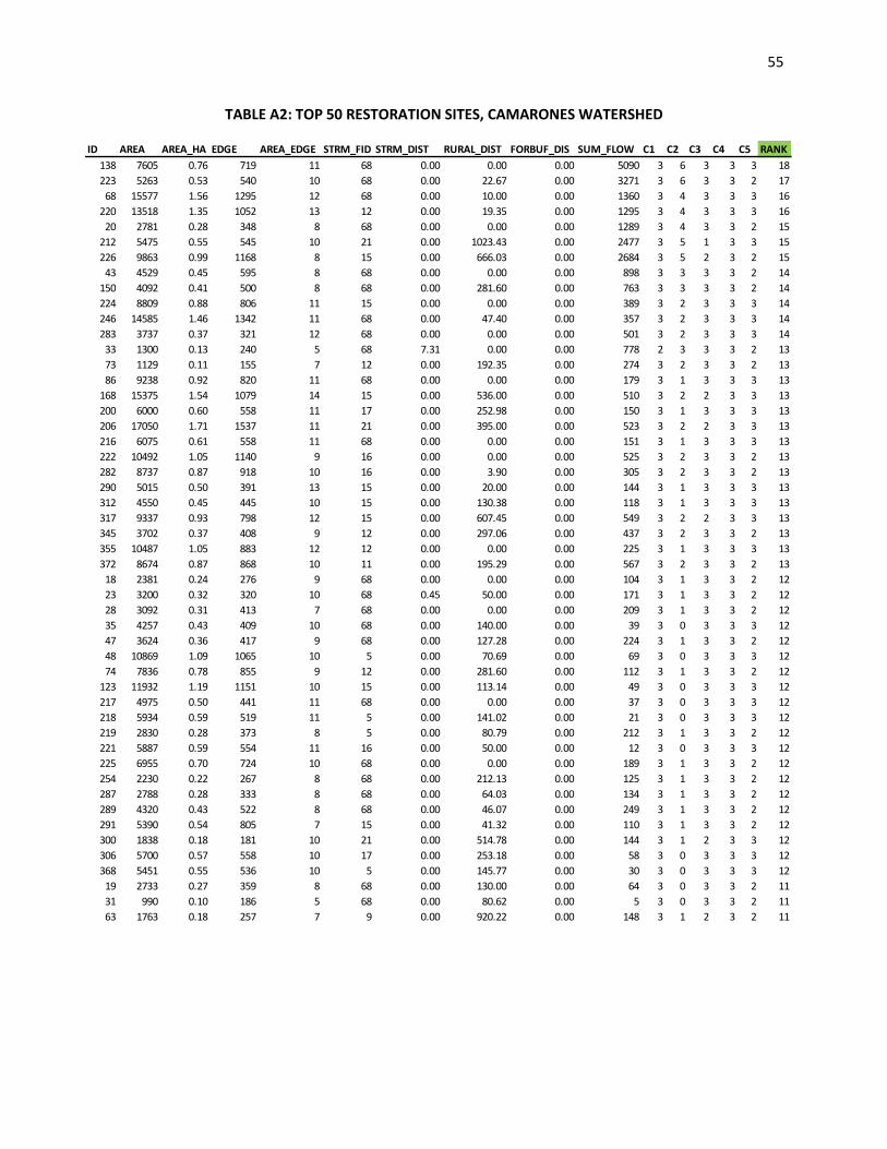
55
TABLE A2: TOP 50 RESTORATION SITES, CAMARONES WATERSHED
ID AREA AREA_HA EDGE AREA_EDGE STRM_FID STRM_DIST RURAL_DIST FORBUF_DIS SUM_FLOW C1 C2 C3 C4 C5 RANK
138 7605 0.76 719 11 68 0.00 0.00 0.00 5090 3 6 3 3 3 18
223 5263 0.53 540 10 68 0.00 22.67 0.00 3271 3 6 3 3 2 17
68 15577 1.56 1295 12 68 0.00 10.00 0.00 1360 3 4 3 3 3 16
220 13518 1.35 1052 13 12 0.00 19.35 0.00 1295 3 4 3 3 3 16
20 2781 0.28 348 8 68 0.00 0.00 0.00 1289 3 4 3 3 2 15
212 5475 0.55 545 10 21 0.00 1023.43 0.00 2477 3 5 1 3 3 15
226 9863 0.99 1168 8 15 0.00 666.03 0.00 2684 3 5 2 3 2 15
43 4529 0.45 595 8 68 0.00 0.00 0.00 898 3 3 3 3 2 14
150 4092 0.41 500 8 68 0.00 281.60 0.00 763 3 3 3 3 2 14
224 8809 0.88 806 11 15 0.00 0.00 0.00 389 3 2 3 3 3 14
246 14585 1.46 1342 11 68 0.00 47.40 0.00 357 3 2 3 3 3 14
283 3737 0.37 321 12 68 0.00 0.00 0.00 501 3 2 3 3 3 14
33 1300 0.13 240 5 68 7.31 0.00 0.00 778 2 3 3 3 2 13
73 1129 0.11 155 7 12 0.00 192.35 0.00 274 3 2 3 3 2 13
86 9238 0.92 820 11 68 0.00 0.00 0.00 179 3 1 3 3 3 13
168 15375 1.54 1079 14 15 0.00 536.00 0.00 510 3 2 2 3 3 13
200 6000 0.60 558 11 17 0.00 252.98 0.00 150 3 1 3 3 3 13
206 17050 1.71 1537 11 21 0.00 395.00 0.00 523 3 2 2 3 3 13
216 6075 0.61 558 11 68 0.00 0.00 0.00 151 3 1 3 3 3 13
222 10492 1.05 1140 9 16 0.00 0.00 0.00 525 3 2 3 3 2 13
282 8737 0.87 918 10 16 0.00 3.90 0.00 305 3 2 3 3 2 13
290 5015 0.50 391 13 15 0.00 20.00 0.00 144 3 1 3 3 3 13
312 4550 0.45 445 10 15 0.00 130.38 0.00 118 3 1 3 3 3 13
317 9337 0.93 798 12 15 0.00 607.45 0.00 549 3 2 2 3 3 13
345 3702 0.37 408 9 12 0.00 297.06 0.00 437 3 2 3 3 2 13
355 10487 1.05 883 12 12 0.00 0.00 0.00 225 3 1 3 3 3 13
372 8674 0.87 868 10 11 0.00 195.29 0.00 567 3 2 3 3 2 13
18 2381 0.24 276 9 68 0.00 0.00 0.00 104 3 1 3 3 2 12
23 3200 0.32 320 10 68 0.45 50.00 0.00 171 3 1 3 3 2 12
28 3092 0.31 413 7 68 0.00 0.00 0.00 209 3 1 3 3 2 12
35 4257 0.43 409 10 68 0.00 140.00 0.00 39 3 0 3 3 3 12
47 3624 0.36 417 9 68 0.00 127.28 0.00 224 3 1 3 3 2 12
48 10869 1.09 1065 10 5 0.00 70.69 0.00 69 3 0 3 3 3 12
74 7836 0.78 855 9 12 0.00 281.60 0.00 112 3 1 3 3 2 12
123 11932 1.19 1151 10 15 0.00 113.14 0.00 49 3 0 3 3 3 12
217 4975 0.50 441 11 68 0.00 0.00 0.00 37 3 0 3 3 3 12
218 5934 0.59 519 11 5 0.00 141.02 0.00 21 3 0 3 3 3 12
219 2830 0.28 373 8 5 0.00 80.79 0.00 212 3 1 3 3 2 12
221 5887 0.59 554 11 16 0.00 50.00 0.00 12 3 0 3 3 3 12
225 6955 0.70 724 10 68 0.00 0.00 0.00 189 3 1 3 3 2 12
254 2230 0.22 267 8 68 0.00 212.13 0.00 125 3 1 3 3 2 12
287 2788 0.28 333 8 68 0.00 64.03 0.00 134 3 1 3 3 2 12
289 4320 0.43 522 8 68 0.00 46.07 0.00 249 3 1 3 3 2 12
291 5390 0.54 805 7 15 0.00 41.32 0.00 110 3 1 3 3 2 12
300 1838 0.18 181 10 21 0.00 514.78 0.00 144 3 1 2 3 3 12
306 5700 0.57 558 10 17 0.00 253.18 0.00 58 3 0 3 3 3 12
368 5451 0.55 536 10 5 0.00 145.77 0.00 30 3 0 3 3 3 12
19 2733 0.27 359 8 68 0.00 130.00 0.00 64 3 0 3 3 2 11
31 990 0.10 186 5 68 0.00 80.62 0.00 5 3 0 3 3 2 11
63 1763 0.18 257 7 9 0.00 920.22 0.00 148 3 1 2 3 2 11
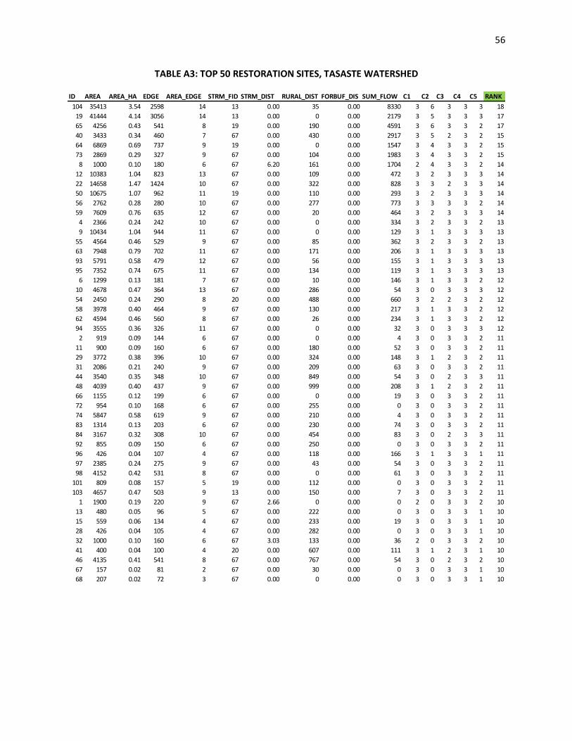
56
TABLE A3: TOP 50 RESTORATION SITES, TASASTE WATERSHED
ID AREA AREA_HA EDGE AREA_EDGE STRM_FID STRM_DIST RURAL_DIST FORBUF_DIS SUM_FLOW C1 C2 C3 C4 C5 RANK
104 35413 3.54 2598 14 13 0.00 35 0.00 8330 3 6 3 3 3 18
19 41444 4.14 3056 14 13 0.00 0 0.00 2179 3 5 3 3 3 17
65 4256 0.43 541 8 19 0.00 190 0.00 4591 3 6 3 3 2 17
40 3433 0.34 460 7 67 0.00 430 0.00 2917 3 5 2 3 2 15
64 6869 0.69 737 9 19 0.00 0 0.00 1547 3 4 3 3 2 15
73 2869 0.29 327 9 67 0.00 104 0.00 1983 3 4 3 3 2 15
8 1000 0.10 180 6 67 6.20 161 0.00 1704 2 4 3 3 2 14
12 10383 1.04 823 13 67 0.00 109 0.00 472 3 2 3 3 3 14
22 14658 1.47 1424 10 67 0.00 322 0.00 828 3 3 2 3 3 14
50 10675 1.07 962 11 19 0.00 110 0.00 293 3 2 3 3 3 14
56 2762 0.28 280 10 67 0.00 277 0.00 773 3 3 3 3 2 14
59 7609 0.76 635 12 67 0.00 20 0.00 464 3 2 3 3 3 14
4 2366 0.24 242 10 67 0.00 0 0.00 334 3 2 3 3 2 13
9 10434 1.04 944 11 67 0.00 0 0.00 129 3 1 3 3 3 13
55 4564 0.46 529 9 67 0.00 85 0.00 362 3 2 3 3 2 13
63 7948 0.79 702 11 67 0.00 171 0.00 206 3 1 3 3 3 13
93 5791 0.58 479 12 67 0.00 56 0.00 155 3 1 3 3 3 13
95 7352 0.74 675 11 67 0.00 134 0.00 119 3 1 3 3 3 13
6 1299 0.13 181 7 67 0.00 10 0.00 146 3 1 3 3 2 12
10 4678 0.47 364 13 67 0.00 286 0.00 54 3 0 3 3 3 12
54 2450 0.24 290 8 20 0.00 488 0.00 660 3 2 2 3 2 12
58 3978 0.40 464 9 67 0.00 130 0.00 217 3 1 3 3 2 12
62 4594 0.46 560 8 67 0.00 26 0.00 234 3 1 3 3 2 12
94 3555 0.36 326 11 67 0.00 0 0.00 32 3 0 3 3 3 12
2 919 0.09 144 6 67 0.00 0 0.00 4 3 0 3 3 2 11
11 900 0.09 160 6 67 0.00 180 0.00 52 3 0 3 3 2 11
29 3772 0.38 396 10 67 0.00 324 0.00 148 3 1 2 3 2 11
31 2086 0.21 240 9 67 0.00 209 0.00 63 3 0 3 3 2 11
44 3540 0.35 348 10 67 0.00 849 0.00 54 3 0 2 3 3 11
48 4039 0.40 437 9 67 0.00 999 0.00 208 3 1 2 3 2 11
66 1155 0.12 199 6 67 0.00 0 0.00 19 3 0 3 3 2 11
72 954 0.10 168 6 67 0.00 255 0.00 0 3 0 3 3 2 11
74 5847 0.58 619 9 67 0.00 210 0.00 4 3 0 3 3 2 11
83 1314 0.13 203 6 67 0.00 230 0.00 74 3 0 3 3 2 11
84 3167 0.32 308 10 67 0.00 454 0.00 83 3 0 2 3 3 11
92 855 0.09 150 6 67 0.00 250 0.00 0 3 0 3 3 2 11
96 426 0.04 107 4 67 0.00 118 0.00 166 3 1 3 3 1 11
97 2385 0.24 275 9 67 0.00 43 0.00 54 3 0 3 3 2 11
98 4152 0.42 531 8 67 0.00 0 0.00 61 3 0 3 3 2 11
101 809 0.08 157 5 19 0.00 112 0.00 0 3 0 3 3 2 11
103 4657 0.47 503 9 13 0.00 150 0.00 7 3 0 3 3 2 11
1 1900 0.19 220 9 67 2.66 0 0.00 0 2 0 3 3 2 10
13 480 0.05 96 5 67 0.00 222 0.00 0 3 0 3 3 1 10
15 559 0.06 134 4 67 0.00 233 0.00 19 3 0 3 3 1 10
28 426 0.04 105 4 67 0.00 282 0.00 0 3 0 3 3 1 10
32 1000 0.10 160 6 67 3.03 133 0.00 36 2 0 3 3 2 10
41 400 0.04 100 4 20 0.00 607 0.00 111 3 1 2 3 1 10
46 4135 0.41 541 8 67 0.00 767 0.00 54 3 0 2 3 2 10
67 157 0.02 81 2 67 0.00 30 0.00 0 3 0 3 3 1 10
68 207 0.02 72 3 67 0.00 0 0.00 0 3 0 3 3 1 10
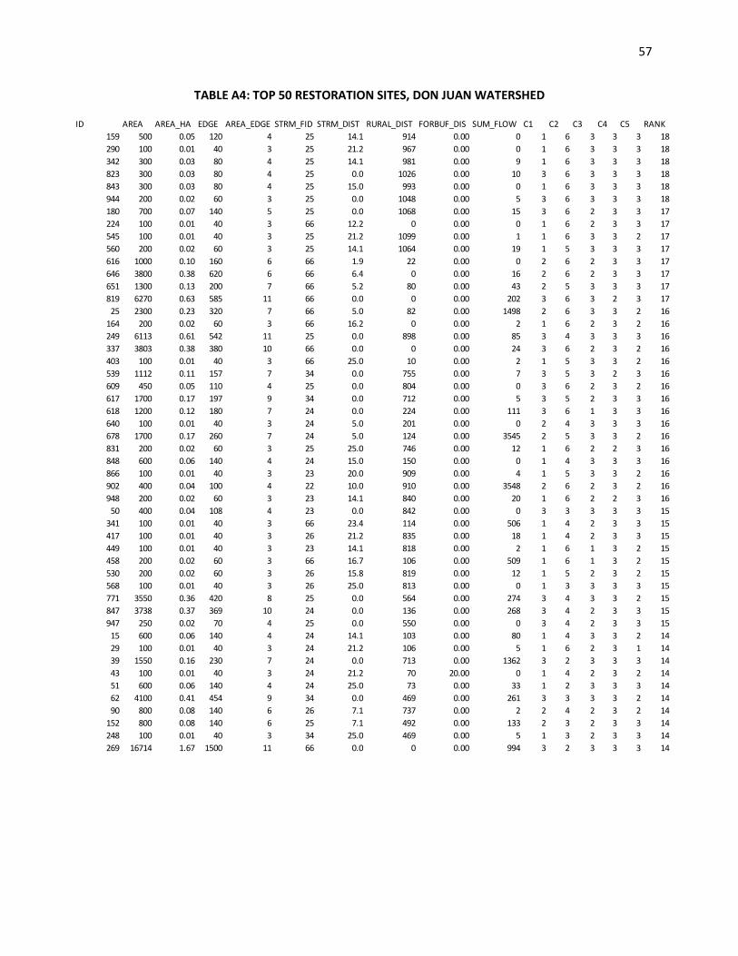
57
TABLE A4: TOP 50 RESTORATION SITES, DON JUAN WATERSHED
ID AREA AREA_HA EDGE AREA_EDGE STRM_FID STRM_DIST RURAL_DIST FORBUF_DIS SUM_FLOW C1 C2 C3 C4 C5 RANK
159 500 0.05 120 4 25 14.1 914 0.00 0 1 6 3 3 3 18
290 100 0.01 40 3 25 21.2 967 0.00 0 1 6 3 3 3 18
342 300 0.03 80 4 25 14.1 981 0.00 9 1 6 3 3 3 18
823 300 0.03 80 4 25 0.0 1026 0.00 10 3 6 3 3 3 18
843 300 0.03 80 4 25 15.0 993 0.00 0 1 6 3 3 3 18
944 200 0.02 60 3 25 0.0 1048 0.00 5 3 6 3 3 3 18
180 700 0.07 140 5 25 0.0 1068 0.00 15 3 6 2 3 3 17
224 100 0.01 40 3 66 12.2 0 0.00 0 1 6 2 3 3 17
545 100 0.01 40 3 25 21.2 1099 0.00 1 1 6 3 3 2 17
560 200 0.02 60 3 25 14.1 1064 0.00 19 1 5 3 3 3 17
616 1000 0.10 160 6 66 1.9 22 0.00 0 2 6 2 3 3 17
646 3800 0.38 620 6 66 6.4 0 0.00 16 2 6 2 3 3 17
651 1300 0.13 200 7 66 5.2 80 0.00 43 2 5 3 3 3 17
819 6270 0.63 585 11 66 0.0 0 0.00 202 3 6 3 2 3 17
25 2300 0.23 320 7 66 5.0 82 0.00 1498 2 6 3 3 2 16
164 200 0.02 60 3 66 16.2 0 0.00 2 1 6 2 3 2 16
249 6113 0.61 542 11 25 0.0 898 0.00 85 3 4 3 3 3 16
337 3803 0.38 380 10 66 0.0 0 0.00 24 3 6 2 3 2 16
403 100 0.01 40 3 66 25.0 10 0.00 2 1 5 3 3 2 16
539 1112 0.11 157 7 34 0.0 755 0.00 7 3 5 3 2 3 16
609 450 0.05 110 4 25 0.0 804 0.00 0 3 6 2 3 2 16
617 1700 0.17 197 9 34 0.0 712 0.00 5 3 5 2 3 3 16
618 1200 0.12 180 7 24 0.0 224 0.00 111 3 6 1 3 3 16
640 100 0.01 40 3 24 5.0 201 0.00 0 2 4 3 3 3 16
678 1700 0.17 260 7 24 5.0 124 0.00 3545 2 5 3 3 2 16
831 200 0.02 60 3 25 25.0 746 0.00 12 1 6 2 2 3 16
848 600 0.06 140 4 24 15.0 150 0.00 0 1 4 3 3 3 16
866 100 0.01 40 3 23 20.0 909 0.00 4 1 5 3 3 2 16
902 400 0.04 100 4 22 10.0 910 0.00 3548 2 6 2 3 2 16
948 200 0.02 60 3 23 14.1 840 0.00 20 1 6 2 2 3 16
50 400 0.04 108 4 23 0.0 842 0.00 0 3 3 3 3 3 15
341 100 0.01 40 3 66 23.4 114 0.00 506 1 4 2 3 3 15
417 100 0.01 40 3 26 21.2 835 0.00 18 1 4 2 3 3 15
449 100 0.01 40 3 23 14.1 818 0.00 2 1 6 1 3 2 15
458 200 0.02 60 3 66 16.7 106 0.00 509 1 6 1 3 2 15
530 200 0.02 60 3 26 15.8 819 0.00 12 1 5 2 3 2 15
568 100 0.01 40 3 26 25.0 813 0.00 0 1 3 3 3 3 15
771 3550 0.36 420 8 25 0.0 564 0.00 274 3 4 3 3 2 15
847 3738 0.37 369 10 24 0.0 136 0.00 268 3 4 2 3 3 15
947 250 0.02 70 4 25 0.0 550 0.00 0 3 4 2 3 3 15
15 600 0.06 140 4 24 14.1 103 0.00 80 1 4 3 3 2 14
29 100 0.01 40 3 24 21.2 106 0.00 5 1 6 2 3 1 14
39 1550 0.16 230 7 24 0.0 713 0.00 1362 3 2 3 3 3 14
43 100 0.01 40 3 24 21.2 70 20.00 0 1 4 2 3 2 14
51 600 0.06 140 4 24 25.0 73 0.00 33 1 2 3 3 3 14
62 4100 0.41 454 9 34 0.0 469 0.00 261 3 3 3 3 2 14
90 800 0.08 140 6 26 7.1 737 0.00 2 2 4 2 3 2 14
152 800 0.08 140 6 25 7.1 492 0.00 133 2 3 2 3 3 14
248 100 0.01 40 3 34 25.0 469 0.00 5 1 3 2 3 3 14
269 16714 1.67 1500 11 66 0.0 0 0.00 994 3 2 3 3 3 14
58
APPENDIX B
Prioritization Model Script: Tabuga Watershed
# -*- coding: utf-8 -*-
# ---------------------------------------------------------------------------
# Prioritization Model.py
# Created on: 2013-04-26 15:42:30.00000
# (generated by ArcGIS/ModelBuilder)
# Description:
# ---------------------------------------------------------------------------
# Import arcpy module
import arcpy
# Local variables:
SitesAll_0312_shp =
"C:\\Users\\Public\\Documents\\MP\\workspace\\data\\Model_Data\\SitesAll_0312.shp"
Jama_LULC_2009 = "Jama_LULC_2009"
ClassificationBoundary = "ClassificationBoundary"
SitesAll_0312 = "SitesAll_0312"
TabugaSites = "TabugaSites"
SitesAll_0312__12_ = "SitesAll_0312"
tmp2009_LULC_shp =
"C:\\Users\\Public\\Documents\\MP\\workspace\\data\\Model_Data\\scratch\\tmp2009_LULC.shp"
v2009_lulc_shp =
"C:\\Users\\Public\\Documents\\MP\\workspace\\data\\Model_Data\\scratch\\2009_lulc.shp"
# Process: Add Field
59
arcpy.AddField_management(SitesAll_0312, "C1", "LONG", "", "", "", "", "NULLABLE", "NON_REQUIRED",
"")
# Process: Add Field (2)
arcpy.AddField_management(SitesAll_0312, "C2", "LONG", "", "", "", "", "NULLABLE", "NON_REQUIRED",
"")
# Process: Add Field (4)
arcpy.AddField_management(SitesAll_0312, "C4", "LONG", "", "", "", "", "NULLABLE", "NON_REQUIRED",
"")
# Process: Add Field (5)
arcpy.AddField_management(SitesAll_0312, "C5", "LONG", "", "", "", "", "NULLABLE", "NON_REQUIRED",
"")
# Process: Add Field (6)
arcpy.AddField_management(SitesAll_0312, "C6", "LONG", "", "", "", "", "NULLABLE", "NON_REQUIRED",
"")
# Process: Calculate Field
arcpy.CalculateField_management(SitesAll_0312__12_, "C1", "Rank( !STRM_DIST!)", "PYTHON_9.3",
"def Rank(x):\\n if x <= 1:\\n return 3\\n elif x <=10:\\n return 2\\n else:\\n return 1")
# Process: Calculate Field (2)
arcpy.CalculateField_management(SitesAll_0312__12_, "C2", "Rank(!RURAL_DIST!)", "PYTHON_9.3",
"def Rank(x):\\n if x <= 300:\\n return 3\\n elif x <=1000:\\n return 2\\n else:\\n return 1")
# Process: Calculate Field (4)
60
arcpy.CalculateField_management(SitesAll_0312__12_, "C4", "Rank( !AREA_EDGE! )", "PYTHON_9.3",
"def Rank(x):\\n if x <= 5:\\n return 1\\n elif x <=10:\\n return 2\\n elif x <=15:\\n return 3\\n")
# Process: Calculate Field (5)
arcpy.CalculateField_management(SitesAll_0312__12_, "C5", "Rank( !FORBUF_DIS!)", "PYTHON_9.3",
"def Rank(x):\\n if x == 0:\\n return 3\\n elif x <=100:\\n return 2\\n else:\\n return 1")
# Process: Raster to Polygon
tempEnvironment0 = arcpy.env.snapRaster
arcpy.env.snapRaster = ""
tempEnvironment1 = arcpy.env.extent
arcpy.env.extent = "584992.934 9974307.889 600472.934 9993807.889"
tempEnvironment2 = arcpy.env.cellSize
arcpy.env.cellSize = "MAXOF"
tempEnvironment3 = arcpy.env.mask
arcpy.env.mask = "watersheds_jolley"
arcpy.RasterToPolygon_conversion(Jama_LULC_2009, tmp2009_LULC_shp, "NO_SIMPLIFY", "Value")
arcpy.env.snapRaster = tempEnvironment0
arcpy.env.extent = tempEnvironment1
arcpy.env.cellSize = tempEnvironment2
arcpy.env.mask = tempEnvironment3
# Process: Clip
arcpy.Clip_analysis(tmp2009_LULC_shp, ClassificationBoundary, v2009_lulc_shp, "")
# Process: Calculate Field (6)
61
arcpy.CalculateField_management(SitesAll_0312__12_, "C6", "Rank( !SUM_FLOW! )", "PYTHON_9.3",
"def Rank(x):\\n if x <= 100:\\n return 0\\n elif x <=250:\\n return 1\\n elif x <=750:\\n return
2\\n elif x <=1000:\\n return 3\\n elif x <=2000:\\n return 4\\n elif x <=3000:\\n return 5\\n
else:\\n return 6")
# Process: Calculate Field (7)
arcpy.CalculateField_management(TabugaSites, "C6", "Rank( !SUM_FLOW! )", "PYTHON_9.3", "def
Rank(x):\\n if x <= 100:\\n return 1\\n elif x <=250:\\n return 2\\n elif x <=500:\\n return 3\\n elif
x <=750:\\n return 4\\n elif x <= 1000:\\n return 5\\n else:\\n return 6")
# Process: Calculate Field (8)
arcpy.CalculateField_management(TabugaSites, "C4", "Rank( !AREA_EDGE! )", "PYTHON_9.3", "def
Rank(x):\\n if x <= 5:\\n return 1\\n elif x <=10:\\n return 2\\n elif x <=15:\\n return 3\\n")